Embed Size (px)
Citation preview
Simple and Efficient Representation of Faults and Fault Transmissibility in a Reservoir Simulator—
Case Study from the Mad Dog Field, Gulf of Mexico
Christopher Walker and Glen Anderson
BP America, 501 Westlake Park Blvd., Houston, Texas 77079
GCAGS Explore & Discover Article #00177* http://www.gcags.org/exploreanddiscover/2016/00177_walker_and_anderson.pdf
Posted September 13, 2016. *Abstract extracted from a full paper appended to this GCAGS Explore & Discover article as a digital addendum to the 2016 volume of the GCAGS Transactions, and delivered as an oral presentation at the 66th Annual GCAGS Convention and 63rd Annual GCSSEPM Meeting in Corpus Christi, Texas, September 18–20, 2016.
ABSTRACT
The Mad Dog Field is one of BP’s largest assets in the Gulf of Mexico, with over 4 billion barrels of oil in place. It was discovered in 1998 and came online in 2005. Fur-ther appraisal success has necessitated the Mad Dog 2 (MD2) development; a second tranche of producers and water injectors tied back to a second floating facility. To cre-ate the predicted production profiles that underpin the economics of the MD2 develop-ment, the Reservoir Management team uses a full field Nexus reservoir simulation mod-el. The Nexus model is upscaled from the RMS geomodel and reflects a snapshot of our Integrated Subsurface Description at a point in time, with structure derived from seis-mic data and geologic and petrophysical properties derived from well results. The long cycle time of seismic processing, seismic interpretation, geomodel building, reservoir model building and finally history matching presents three challenges to the representa-tion of faults in the dynamic simulator: Location, Transmissibility, and Presence. This article discusses how we have met these challenges in Mad Dog.
Originally published as: Walker, C. D., and G. A. Anderson, 2016, Simple and efficient representation of faults and fault transmissibility in a reservoir simulator: Case study from the Mad Dog Field, Gulf of Mexico: Gulf Coast Association of Geological Societies Transactions, v. 66, p. 1109–1116.
1

Reservoir Management
progressing resources, delivering production
Using Fault Transmissibility to Assess
Compartmentalization and Forecast
Reservoir Performance in the Mad
Dog Field, Gulf of Mexico, USA
Chris Walker and Glen Anderson
GCAGS Corpus Christi
20th
September 2016
Reservoir Management progressing resources, delivering production
2
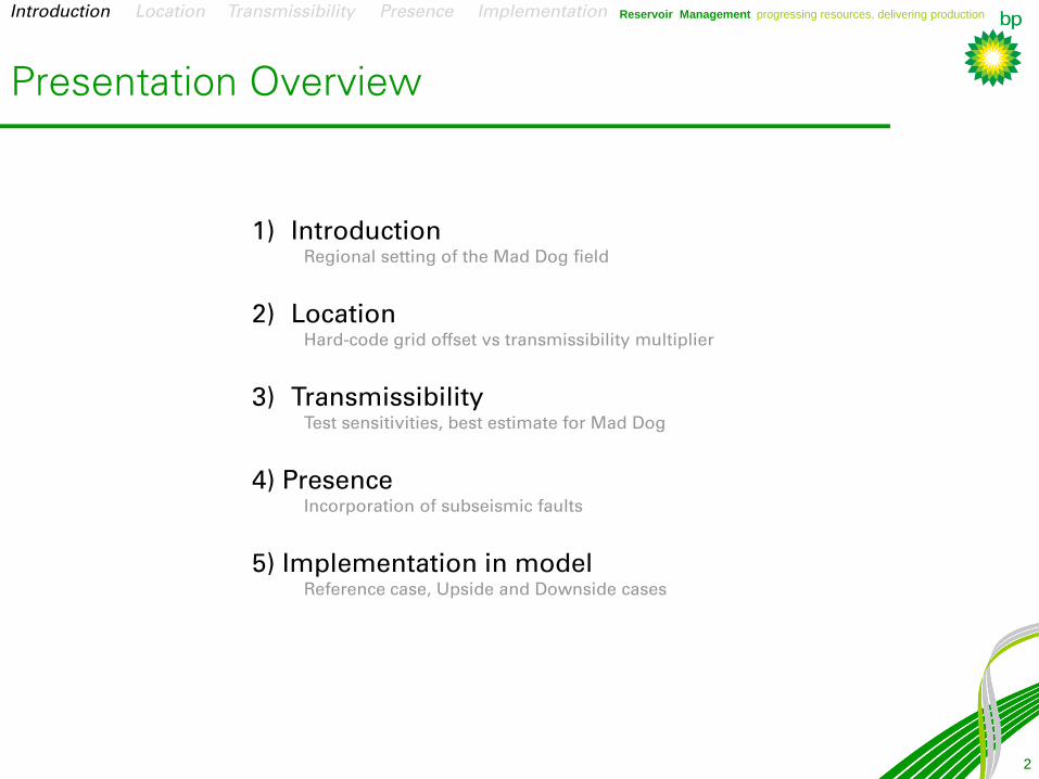
Presentation Overview
1) Introduction
Regional setting of the Mad Dog field
2) Location
Hard-code grid offset vs transmissibility multiplier
3) Transmissibility
Test sensitivities, best estimate for Mad Dog
4) Presence
Incorporation of subseismic faults
5) Implementation in model
Reference case, Upside and Downside cases
Introduction Location Transmissibility Presence Implementation
Reservoir Management progressing resources, delivering production
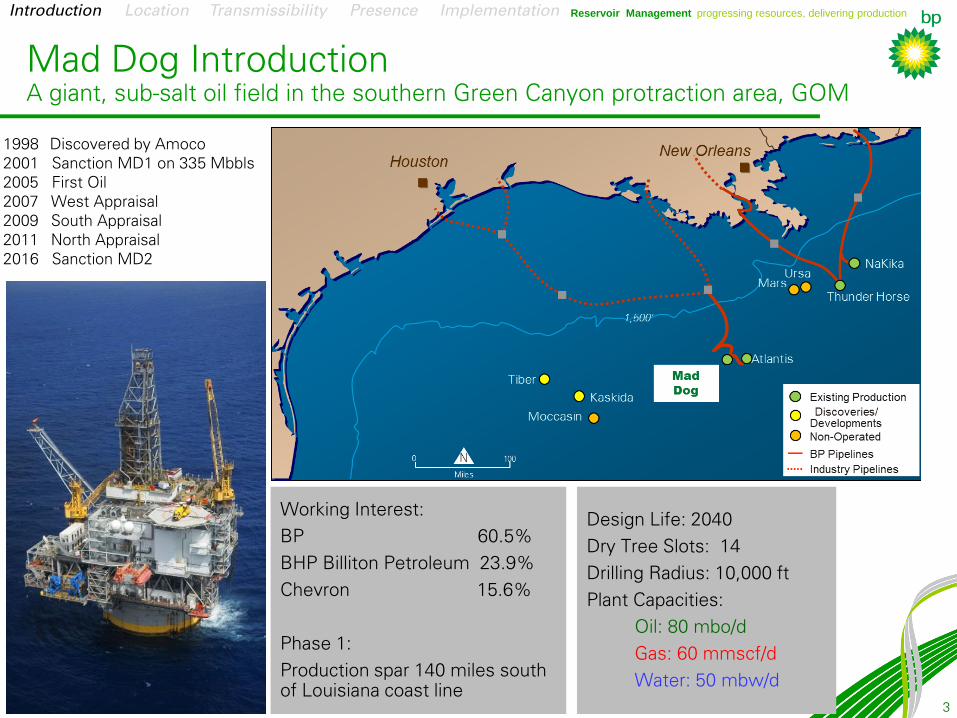
Mad Dog Introduction
A giant, sub-salt oil field in the southern Green Canyon protraction area, GOM
3
Design Life: 2040
Dry Tree Slots: 14
Drilling Radius: 10,000 ft
Plant Capacities:
Oil: 80 mbo/d
Gas: 60 mmscf/d
Water: 50 mbw/d
1998 Discovered by Amoco
2001 Sanction MD1 on 335 Mbbls
2005 First Oil
2007 West Appraisal
2009 South Appraisal
2011 North Appraisal
2016 Sanction MD2
Working Interest:
BP 60.5%
BHP Billiton Petroleum 23.9%
Chevron 15.6%
Phase 1:
Production spar 140 miles south
of Louisiana coast line
Introduction Location Transmissibility Presence Implementation
Reservoir Management progressing resources, delivering production
4
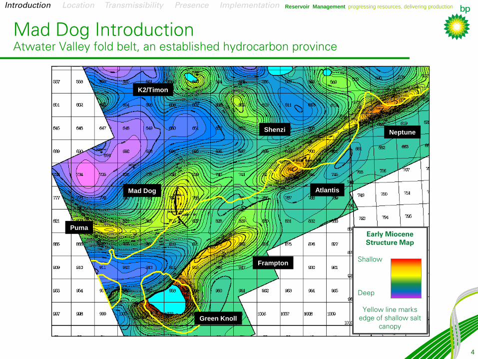
Green Knoll
Frampton
K2/Timon
Shenzi Neptune
Atlantis Mad Dog
Puma Early Miocene
Structure Map
Shallow
Deep
Yellow line marks
edge of shallow salt
canopy
Mad Dog Introduction
Atwater Valley fold belt, an established hydrocarbon province
Introduction Location Transmissibility Presence Implementation
Reservoir Management progressing resources, delivering production
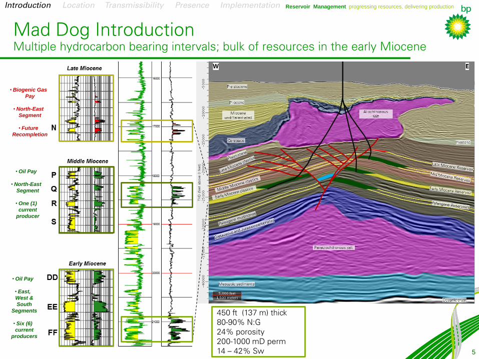
Mad Dog Introduction
Multiple hydrocarbon bearing intervals; bulk of resources in the early Miocene
• Oil Pay
• East,
West &
South
Segments
• Six (6)
current
producers
• Oil Pay
• North-East
Segment
• One (1)
current
producer
• Biogenic Gas
Pay
• North-East
Segment
• Future
Recompletion
450 ft (137 m) thick
80-90% N:G
24% porosity
200-1000 mD perm
14 – 42% Sw 5
Introduction Location Transmissibility Presence Implementation
Reservoir Management progressing resources, delivering production
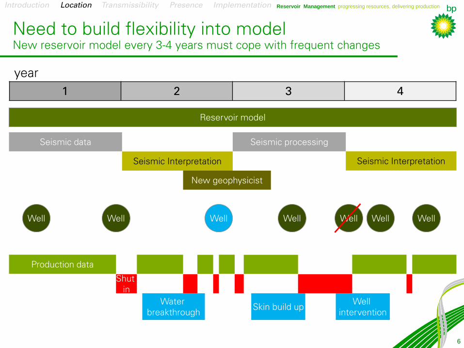
Need to build flexibility into model
New reservoir model every 3-4 years must cope with frequent changes
6
Introduction Location Transmissibility Presence Implementation
1 2 3 4
Reservoir model
year
Seismic data Seismic processing
Seismic Interpretation Seismic Interpretation
Well Well Well Well Well Well
Production data
Shut
in
New geophysicist
Water
breakthrough
Well
Skin build up Well
intervention

Reservoir Management progressing resources, delivering production
Need to build flexibility into model
Review of Mad Dog maps through time shows frequent changes
7
Introduction Location Transmissibility Presence Implementation
Reservoir Management progressing resources, delivering production
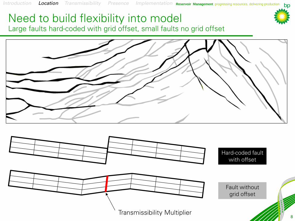
Need to build flexibility into model
Large faults hard-coded with grid offset, small faults no grid offset
8
Hard-coded fault
with offset
Fault without
grid offset
Transmissibility Multiplier
Introduction Location Transmissibility Presence Implementation
Reservoir Management progressing resources, delivering production
9
DD
EE
FF
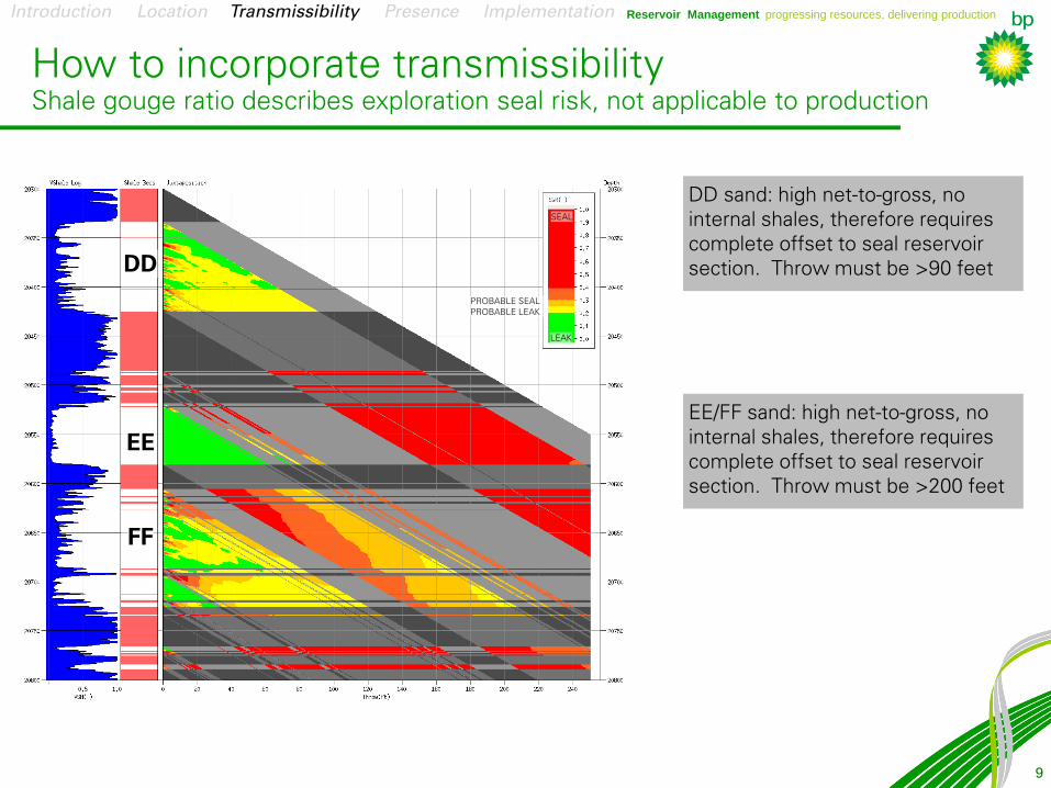
DD sand: high net-to-gross, no
internal shales, therefore requires
complete offset to seal reservoir
section. Throw must be >90 feet
SEAL
PROBABLE SEAL
LEAK
PROBABLE LEAK
EE/FF sand: high net-to-gross, no
internal shales, therefore requires
complete offset to seal reservoir
section. Throw must be >200 feet
How to incorporate transmissibility
Shale gouge ratio describes exploration seal risk, not applicable to production
Introduction Location Transmissibility Presence Implementation
Reservoir Management progressing resources, delivering production
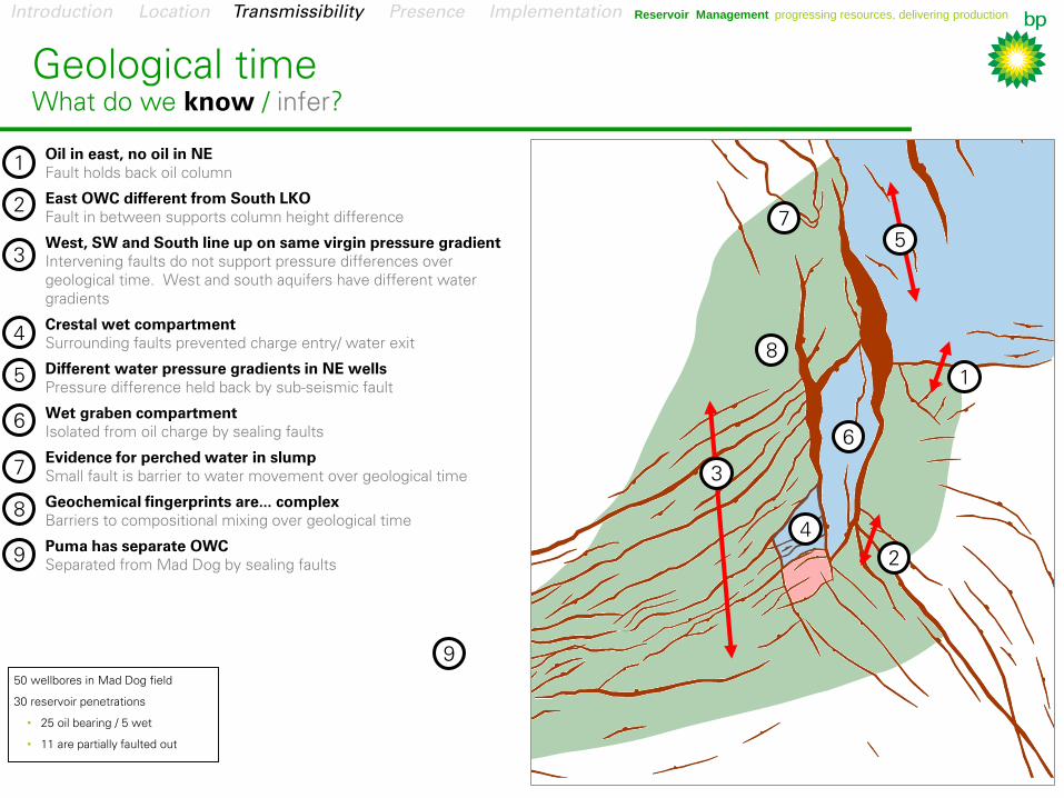
50 wellbores in Mad Dog field
30 reservoir penetrations
• 25 oil bearing / 5 wet
• 11 are partially faulted out
1
2
3
4
5
6
8
7
9
Geological time
What do we know / infer?
Oil in east, no oil in NE
Fault holds back oil column
East OWC different from South LKO
Fault in between supports column height difference
West, SW and South line up on same virgin pressure gradient
Intervening faults do not support pressure differences over
geological time. West and south aquifers have different water
gradients
Crestal wet compartment
Surrounding faults prevented charge entry/ water exit
Different water pressure gradients in NE wells
Pressure difference held back by sub-seismic fault
Wet graben compartment
Isolated from oil charge by sealing faults
Evidence for perched water in slump
Small fault is barrier to water movement over geological time
Geochemical fingerprints are... complex
Barriers to compositional mixing over geological time
Puma has separate OWC
Separated from Mad Dog by sealing faults
1
2
3
4
5
6
7
8
9
Introduction Location Transmissibility Presence Implementation
Reservoir Management progressing resources, delivering production
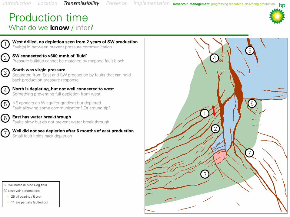
50 wellbores in Mad Dog field
30 reservoir penetrations
• 25 oil bearing / 5 wet
• 11 are partially faulted out
West drilled, no depletion seen from 2 years of SW production
Fault(s) in between prevent pressure communication
SW connected to >600 mmb of ‘fluid’
Pressure buildup cannot be matched by mapped fault block
South was virgin pressure
Separated from East and SW production by faults that can hold
back production pressure response
North is depleting, but not well connected to west
Something preventing full depletion from west
NE appears on W aquifer gradient but depleted
Fault allowing some communication? Or around tip?
East has water breakthrough
Faults slow but do not prevent water break-through
Well did not see depletion after 6 months of east production
Small fault holds back depletion
1
2
3
4
5
6
7
Production time
What do we know / infer?
1
7
3
4
5
6
2
Introduction Location Transmissibility Presence Implementation
Reservoir Management progressing resources, delivering production
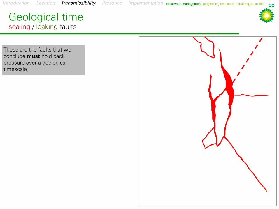
These are the faults that we
conclude must hold back
pressure over a geological
timescale
Geological time
sealing / leaking faults
Introduction Location Transmissibility Presence Implementation

Reservoir Management progressing resources, delivering production
These are the faults that we
conclude must hold back
pressure over a geological
timescale
...and
The faults that we conclude
must not hold back pressure
over a geological timescale
Geological time
sealing / leaking faults
Introduction Location Transmissibility Presence Implementation
Reservoir Management progressing resources, delivering production
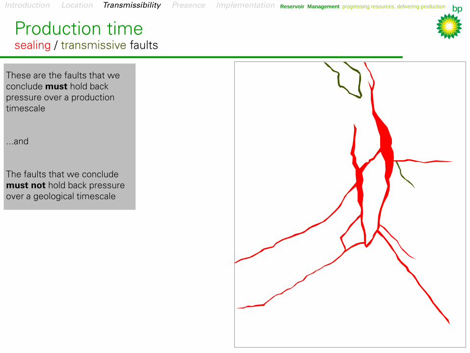
Production time
sealing / transmissive faults
These are the faults that we
conclude must hold back
pressure over a production
timescale
...and
The faults that we conclude
must not hold back pressure
over a geological timescale
Introduction Location Transmissibility Presence Implementation
Reservoir Management progressing resources, delivering production
15
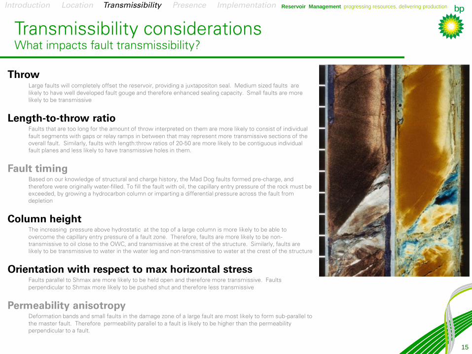
Throw
Large faults will completely offset the reservoir, providing a juxtapositon seal. Medium sized faults are
likely to have well developed fault gouge and therefore enhanced sealing capacity. Small faults are more
likely to be transmissive
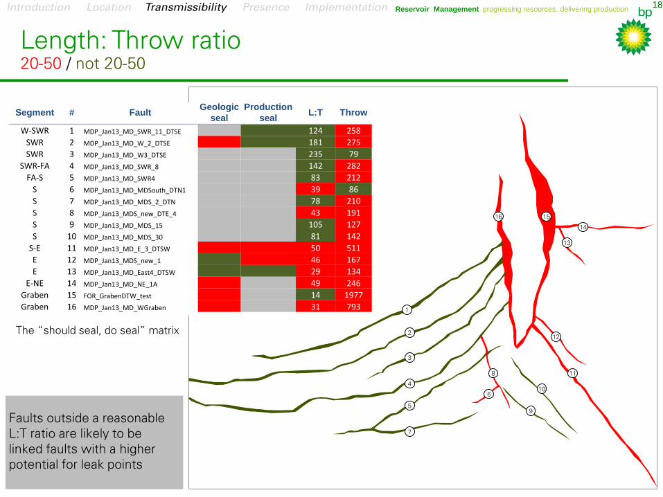
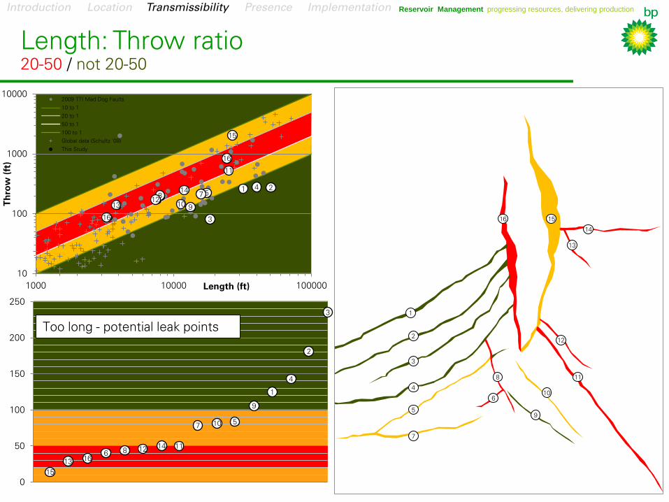
Length-to-throw ratio
Faults that are too long for the amount of throw interpreted on them are more likely to consist of individual
fault segments with gaps or relay ramps in between that may represent more transmissive sections of the
overall fault. Similarly, faults with length:throw ratios of 20-50 are more likely to be contiguous individual
fault planes and less likely to have transmissive holes in them.
Fault timing
Based on our knowledge of structural and charge history, the Mad Dog faults formed pre-charge, and
therefore were originally water-filled. To fill the fault with oil, the capillary entry pressure of the rock must be
exceeded, by growing a hydrocarbon column or imparting a differential pressure across the fault from
depletion
Column height
The increasing pressure above hydrostatic at the top of a large column is more likely to be able to
overcome the capillary entry pressure of a fault zone. Therefore, faults are more likely to be non-
transmissive to oil close to the OWC, and transmissive at the crest of the structure. Similarly, faults are
likely to be transmissive to water in the water leg and non-transmissive to water at the crest of the structure
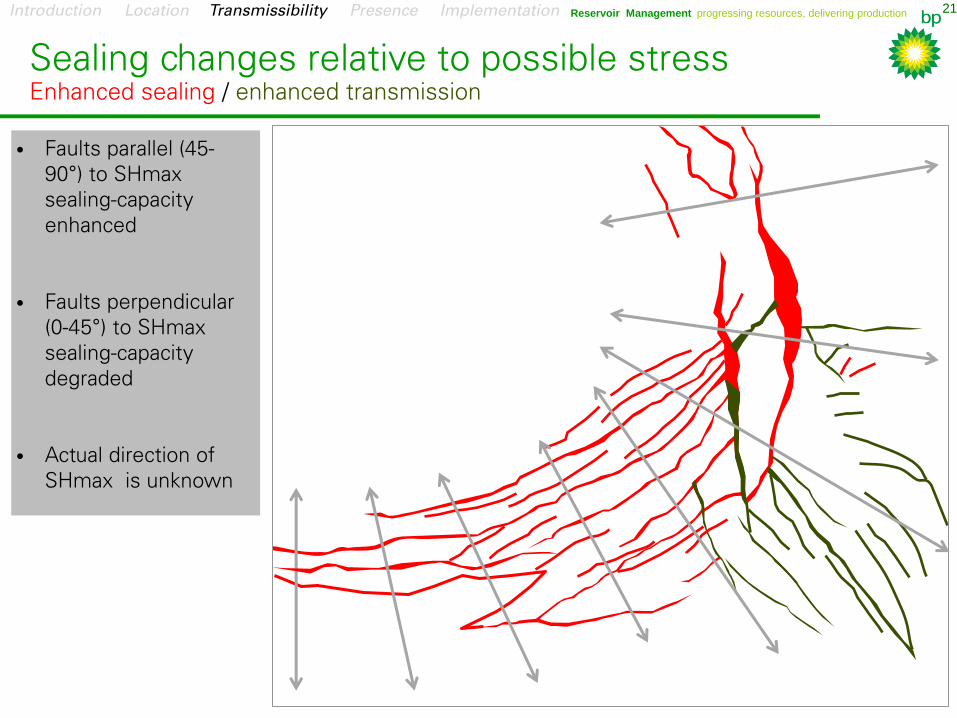
Orientation with respect to max horizontal stress
Faults parallel to Shmax are more likely to be held open and therefore more transmissive. Faults
perpendicular to Shmax more likely to be pushed shut and therefore less transmissive
Permeability anisotropy
Deformation bands and small faults in the damage zone of a large fault are most likely to form sub-parallel to
the master fault. Therefore permeability parallel to a fault is likely to be higher than the permeability
perpendicular to a fault.
Transmissibility considerations
What impacts fault transmissibility?
Introduction Location Transmissibility Presence Implementation
Reservoir Management progressing resources, delivering production
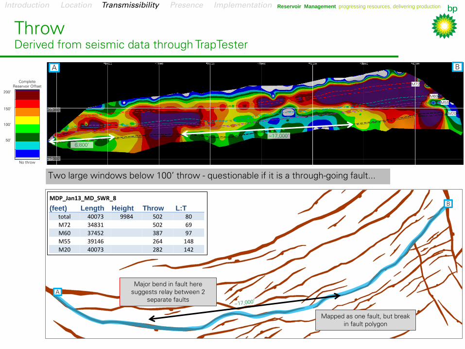
B
A
B
Complete
Reservoir Offset
100’
50’
150’
No throw
200’
Two large windows below 100’ throw - questionable if it is a through-going fault...
A
20,000’
25,000’
M55
M20
M60
M72
~17,000’
Mapped as one fault, but break
in fault polygon
Major bend in fault here
suggests relay between 2
separate faults
6,800’
MDP_Jan13_MD_SWR_8
(feet) Length Height Throw L:T total 40073 9984 502 80
M72 34831 502 69
M60 37452 387 97
M55 39146 264 148
M20 40073 282 142
Throw
Derived from seismic data through TrapTester
Introduction Location Transmissibility Presence Implementation
Reservoir Management progressing resources, delivering production
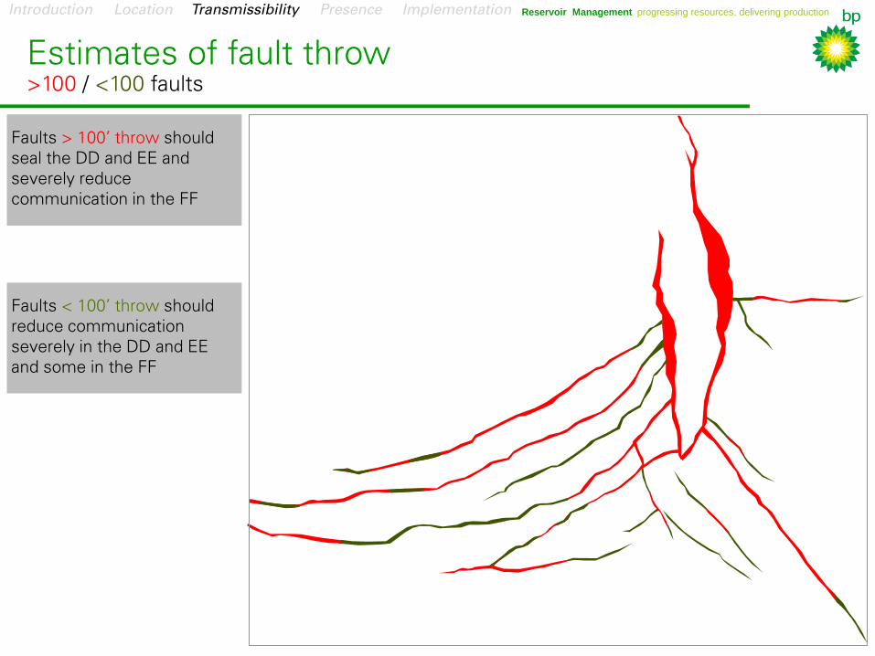
Estimates of fault throw
>100 / <100 faults
Faults > 100’ throw should
seal the DD and EE and
severely reduce
communication in the FF
Faults < 100’ throw should
reduce communication
severely in the DD and EE
and some in the FF
Introduction Location Transmissibility Presence Implementation
Reservoir Management progressing resources, delivering production 18
1
2
3
4
5
6
7
8
9
10
11
12
13
14
15 16
Segment # Fault Geologic
seal
Production
seal L:T Throw
W-SWR 1 MDP_Jan13_MD_SWR_11_DTSE 124 258
SWR 2 MDP_Jan13_MD_W_2_DTSE 181 275
SWR 3 MDP_Jan13_MD_W3_DTSE 235 79
SWR-FA 4 MDP_Jan13_MD_SWR_8 142 282
FA-S 5 MDP_Jan13_MD_SWR4 83 212
S 6 MDP_Jan13_MD_MDSouth_DTN1 39 86
S 7 MDP_Jan13_MD_MDS_2_DTN 78 210
S 8 MDP_Jan13_MDS_new_DTE_4 43 191
S 9 MDP_Jan13_MD_MDS_15 105 127
S 10 MDP_Jan13_MD_MDS_30 81 142
S-E 11 MDP_Jan13_MD_E_3_DTSW 50 511
E 12 MDP_Jan13_MDS_new_1 46 167
E 13 MDP_Jan13_MD_East4_DTSW 29 134
E-NE 14 MDP_Jan13_MD_NE_1A 49 246
Graben 15 FOR_GrabenDTW_test 14 1977
Graben 16 MDP_Jan13_MD_WGraben 31 793
The “should seal, do seal” matrix
Faults outside a reasonable
L:T ratio are likely to be
linked faults with a higher
potential for leak points
Length: Throw ratio
20-50 / not 20-50
Introduction Location Transmissibility Presence Implementation
Reservoir Management progressing resources, delivering production
Length: Throw ratio
20-50 / not 20-50
1
2
3
4
5
6
7
8
9
10
11
12
13
14
15 16
0
50
100
150
200
250
15
13 16
6 8 12
14 11
7 10 5
9
1
4
2
3
Too long - potential leak points
10
100
1000
10000
1000 10000 100000
Th
ro
w (ft)
Length (ft)
2009 TTI Mad Dog Faults
10 to 1
20 to 1
50 to 1
100 to 1
Global data (Schultz '08)
This Study
16
2 4 1
15
11
16
3
5 7
9
14
10
8 12
13
Introduction Location Transmissibility Presence Implementation

Reservoir Management progressing resources, delivering production
20
from Fisher and Jolley (2007):
Treatment of Faults in Production Simulation Models,
Geological Society of London, Special Publications 2007,
v.292; p. 219-233. doi: 10.1144/SP292.13
Faults behave like a zone of poor quality rock,
therefore will have a transition zone further above
the FWL than good quality reservoir rock
• Faults are more likely to be non-transmissive to oil close
to the OWC, and transmissive at the crest of the
structure
• Faults are likely to be transmissive to water in the water
leg and non-transmissive to water at the crest of the
structure
• Calculation using Mad Dog rocks suggest OWC in faults
likely to be >1000’ higher than FWL in reservoir rock
Sealing capability of faults
Faults act as a “wall of water”
Introduction Location Transmissibility Presence Implementation
Reservoir Management progressing resources, delivering production 21
• Faults parallel (45-
90°) to SHmax
sealing-capacity
enhanced
• Faults perpendicular
(0-45°) to SHmax
sealing-capacity
degraded
• Actual direction of
SHmax is unknown
Sealing changes relative to possible stress
Enhanced sealing / enhanced transmission
Introduction Location Transmissibility Presence Implementation
Reservoir Management progressing resources, delivering production
22
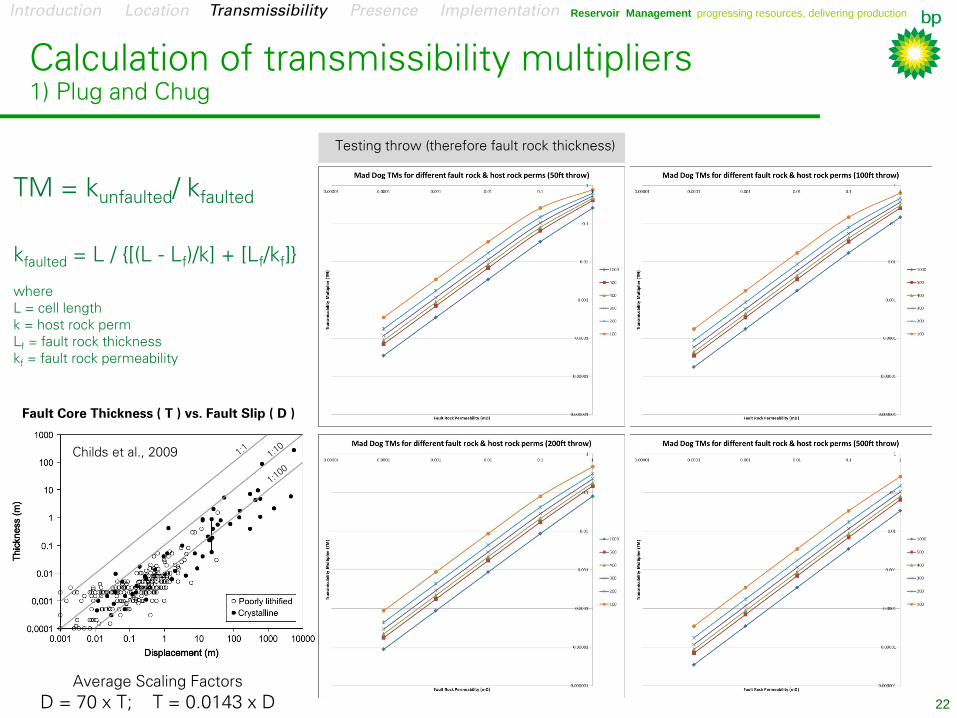
Calculation of transmissibility multipliers
1) Plug and Chug
kfaulted
= L / {[(L - Lf)/k] + [L
f/k
f]}
where
L = cell length
k = host rock perm
Lf = fault rock thickness
kf = fault rock permeability
TM = kunfaulted
/ kfaulted
Testing throw (therefore fault rock thickness)
Average Scaling Factors
D = 70 x T; T = 0.0143 x D
Childs et al., 2009
Fault Core Thickness ( T ) vs. Fault Slip ( D )
Introduction Location Transmissibility Presence Implementation

Reservoir Management progressing resources, delivering production
Calculation of transmissibility multipliers
2) Test Sensitivities
kfaulted
= L / {[(L - Lf)/k] + [L
f/k
f]}
where
L = cell length
k = host rock perm
Lf = fault rock thickness
kf = fault rock permeability
TM = kunfaulted
/ kfaulted
Testing throw (constant host rock perm) Testing fault rock thickness Testing grid cell length
Introduction Location Transmissibility Presence Implementation

Reservoir Management progressing resources, delivering production
Calculation of transmissibility multipliers
3) Define best estimate for Mad Dog
kfaulted
= L / {[(L - Lf)/k] + [L
f/k
f]}
where
L = cell length
k = host rock perm
Lf = fault rock thickness
kf = fault rock permeability
TM = kunfaulted
/ kfaulted
Range of fault perms
Range of Transm
issib
ility
Multip
liers
Measured values from Mad Dog core
Introduction Location Transmissibility Presence Implementation
Reservoir Management progressing resources, delivering production
25
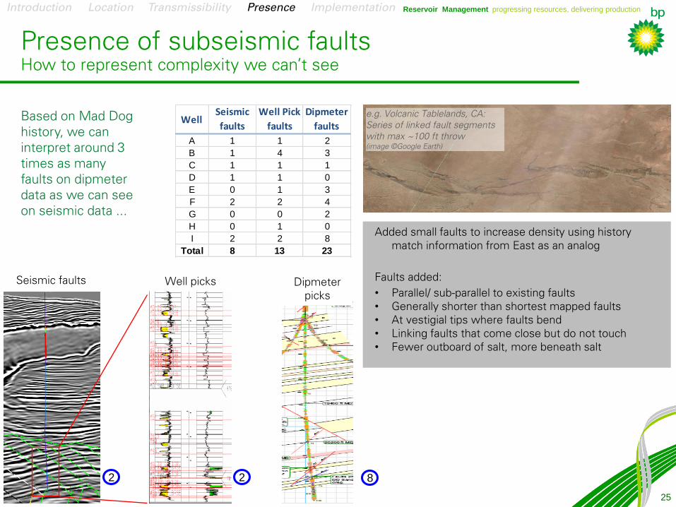
Presence of subseismic faults
How to represent complexity we can’t see
Based on Mad Dog
history, we can
interpret around 3
times as many
faults on dipmeter
data as we can see
on seismic data ...
Added small faults to increase density using history
match information from East as an analog
Faults added:
• Parallel/ sub-parallel to existing faults
• Generally shorter than shortest mapped faults
• At vestigial tips where faults bend
• Linking faults that come close but do not touch
• Fewer outboard of salt, more beneath salt
e.g. Volcanic Tablelands, CA:
Series of linked fault segments
with max ~100 ft throw
(image ©Google Earth)
2
Seismic faults Well picks Dipmeter
picks
2 8
WellSeismic
faults
Well Pick
faults
Dipmeter
faults
A 1 1 2
B 1 4 3
C 1 1 1
D 1 1 0
E 0 1 3
F 2 2 4
G 0 0 2
H 0 1 0
I 2 2 8
Total 8 13 23
Introduction Location Transmissibility Presence Implementation
Reservoir Management progressing resources, delivering production
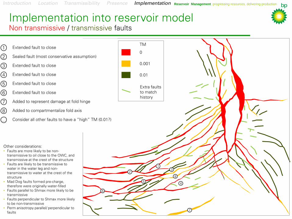
Other considerations:
• Faults are more likely to be non-
transmissive to oil close to the OWC, and
transmissive at the crest of the structure
• Faults are likely to be transmissive to
water in the water leg and non-
transmissive to water at the crest of the
structure
• Mad Dog faults formed pre-charge,
therefore were originally water-filled
• Faults parallel to Shmax more likely to be
transmissive
• Faults perpendicular to Shmax more likely
to be non-transmissive
• Perm anisotropy parallel/ perpendicular to
faults
4
7
1
5
2
8
6
3
0
0.01
TM
0.001
Extra faults
to match
history
Implementation into reservoir model
Non transmissive / transmissive faults
Extended fault to close
Sealed fault (most conservative assumption)
Extended fault to close
Extended fault to close
Extended fault to close
Extended fault to close
Added to represent damage at fold hinge
Added to compartmentalize fold axis
Consider all other faults to have a “high” TM (0.01?)
1
2
3
4
5
6
7
8
...
Introduction Location Transmissibility Presence Implementation
Reservoir Management progressing resources, delivering production
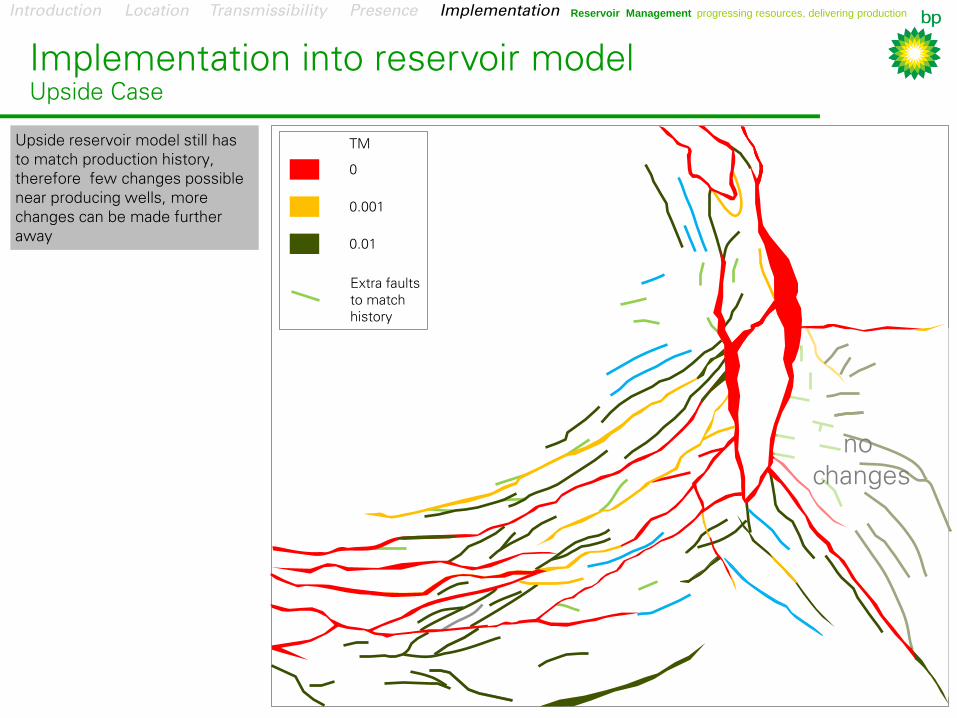
Implementation into reservoir model
Upside Case
no
changes
0
0.01
TM
0.001
Extra faults
to match
history
Introduction Location Transmissibility Presence Implementation
Upside reservoir model still has
to match production history,
therefore few changes possible
near producing wells, more
changes can be made further
away
Reservoir Management progressing resources, delivering production
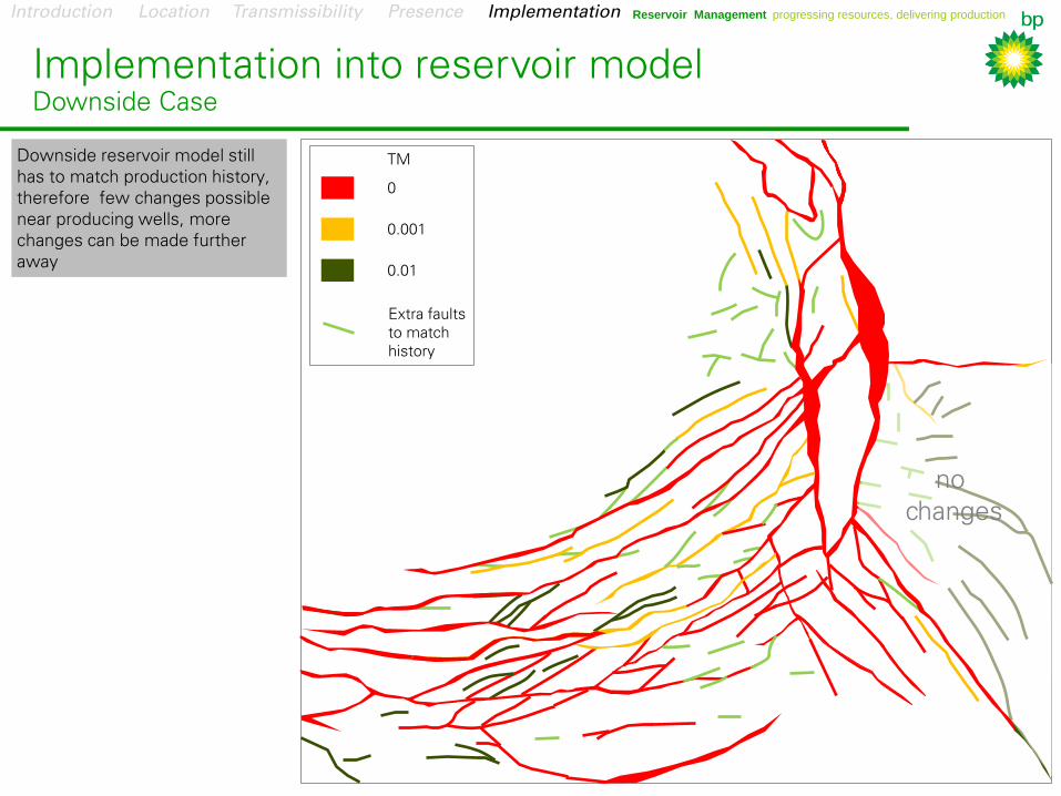
Implementation into reservoir model
Downside Case
no
changes
0
0.01
TM
0.001
Extra faults
to match
history
Introduction Location Transmissibility Presence Implementation
Downside reservoir model still
has to match production history,
therefore few changes possible
near producing wells, more
changes can be made further
away

Reservoir Management progressing resources, delivering production
Building a better reservoir model
Start with seismic map and add geology
Downside realization Upside realization
Reference realization
Seismically-derived map • Begin with the seismically defined
top reservoir structure map
• Amend to match static and
dynamic pressure data
• Decision must be made about the
transmissive properties of each
fault.
Major concerns
• Location
• Transmissibility
• Presence
Upside changes
• Fault transmissivity increased
• No isolated compartments
• High L:T mapped faults segmented
• Fewer sub-seismic faults
Downside changes
• Fault transmissivity decreased
• More isolated compartments
• Mapped faults lengthened
• More sub-seismic faults
Seal
Heavy Baffle
Light Baffle
Added faults to
increase density
Open
Introduction Location Transmissibility Presence Implementation
Reservoir Management progressing resources, delivering production
30
References
Brenner, N., 2011, BHP drills sidetracks to extend Mad Dog appraisal: Upstream Magazine, 25th November 2011. Bretan, P., G. Yielding, and H. Jones, 2003, Using calibrated shale gouge ratio to estimate hydrocarbon column heights: American
Association of Petroleum Geologists Bulletin, v. 87, no. 3, p. 397–413 Childs, C., T. Manzocchi, J. J. Walsh, C. G. Bonson, A. Nicol, and M. P. G. Schöpfer, 2009, A geometric model of fault zone and fault
rock thickness variations: Journal of Structural Geology, v. 31, p. 117–127. Fisher Q. J. and S.J. Jolley, 2007, Treatment of Faults in Production Simulation Models, in Jolley, S. J., D. Barr, J. J. Walsh, and R. J.
Knipe, (eds) Structurally Complex Reservoirs: Geological Society, London, Special Publications, 292, p.219–233. doi: 10.1144/SP292.13
Walker, C.D., P. Belvedere, J. Petersen, S. Warrior, A. Cunningham, G. Clemenceau, C. Huenink, and R. Meltz, 2012, Straining at the
leash: Understanding the full potential of the deepwater, sub-salt Mad Dog field, from appraisal through early production, in N. C. Rosen et al., eds., New Understanding of the Petroleum Systems of Continental Margins of the World: 32nd Annual Gulf Coast Section Society of Economic Paleontologists and Mineralogists Foundation Bob F. Perkins Research Conference, v. 32, p. 25–64.
Walker, C. D., G. A. Anderson, P. G. Belvedere, A. T. Henning, F. O. Rollins, E. Soza, and S. Warrior, 2015, Compartmentalization
between the GC0738_1 Mad Dog North wellbores - Evidence for post-depositional slumping in the Lower Miocene reservoirs of the deepwater southern Green Canyon, Gulf of Mexico: Gulf Coast Association of Geological Societies Transactions, v. 65, p. 389–402.
Simple and Efficient Representation of Faults and Fault Transmissibility in a Reservoir Simulator:
Case Study from the Mad Dog Field, Gulf of Mexico
Christopher D. Walker and Glen A. Anderson
BP America, 501 Westlake Park Blvd., Houston, Texas 77079
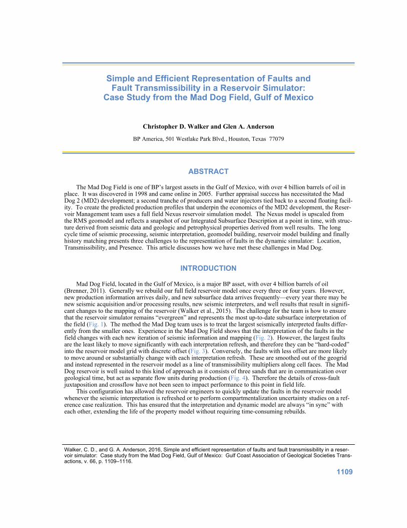
ABSTRACT The Mad Dog Field is one of BP’s largest assets in the Gulf of Mexico, with over 4 billion barrels of oil in
place. It was discovered in 1998 and came online in 2005. Further appraisal success has necessitated the Mad Dog 2 (MD2) development; a second tranche of producers and water injectors tied back to a second floating facil-ity. To create the predicted production profiles that underpin the economics of the MD2 development, the Reser-voir Management team uses a full field Nexus reservoir simulation model. The Nexus model is upscaled from the RMS geomodel and reflects a snapshot of our Integrated Subsurface Description at a point in time, with struc-ture derived from seismic data and geologic and petrophysical properties derived from well results. The long cycle time of seismic processing, seismic interpretation, geomodel building, reservoir model building and finally history matching presents three challenges to the representation of faults in the dynamic simulator: Location, Transmissibility, and Presence. This article discusses how we have met these challenges in Mad Dog.
INTRODUCTION Mad Dog Field, located in the Gulf of Mexico, is a major BP asset, with over 4 billion barrels of oil
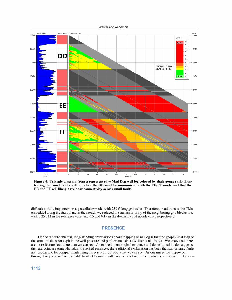
(Brenner, 2011). Generally we rebuild our full field reservoir model once every three or four years. However, new production information arrives daily, and new subsurface data arrives frequently—every year there may be new seismic acquisition and/or processing results, new seismic interpreters, and well results that result in signifi-cant changes to the mapping of the reservoir (Walker et al., 2015). The challenge for the team is how to ensure that the reservoir simulator remains “evergreen” and represents the most up-to-date subsurface interpretation of the field (Fig. 1). The method the Mad Dog team uses is to treat the largest seismically interpreted faults differ-ently from the smaller ones. Experience in the Mad Dog Field shows that the interpretation of the faults in the field changes with each new iteration of seismic information and mapping (Fig. 2). However, the largest faults are the least likely to move significantly with each interpretation refresh, and therefore they can be “hard-coded” into the reservoir model grid with discrete offset (Fig. 3). Conversely, the faults with less offset are more likely to move around or substantially change with each interpretation refresh. These are smoothed out of the geogrid and instead represented in the reservoir model as a line of transmissibility multipliers along cell faces. The Mad Dog reservoir is well suited to this kind of approach as it consists of three sands that are in communication over geological time, but act as separate flow units during production (Fig. 4). Therefore the details of cross-fault juxtaposition and crossflow have not been seen to impact performance to this point in field life.
This configuration has allowed the reservoir engineers to quickly update the faults in the reservoir model whenever the seismic interpretation is refreshed or to perform compartmentalization uncertainty studies on a ref-erence case realization. This has ensured that the interpretation and dynamic model are always “in sync” with each other, extending the life of the property model without requiring time-consuming rebuilds.
Walker, C. D., and G. A. Anderson, 2016, Simple and efficient representation of faults and fault transmissibility in a reser-voir simulator: Case study from the Mad Dog Field, Gulf of Mexico: Gulf Coast Association of Geological Societies Trans-actions, v. 66, p. 1109–1116.
1109
Walker and Anderson
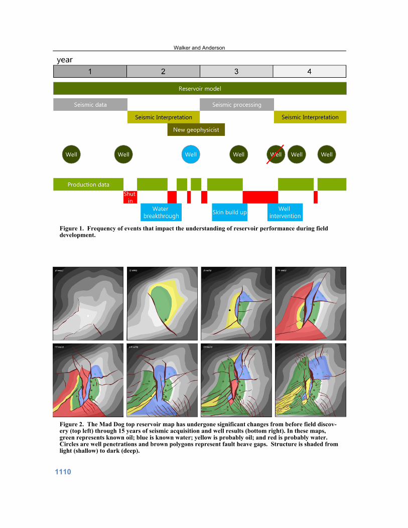
Figure 1. Frequency of events that impact the understanding of reservoir performance during field development.
Figure 2. The Mad Dog top reservoir map has undergone significant changes from before field discov-ery (top left) through 15 years of seismic acquisition and well results (bottom right). In these maps, green represents known oil; blue is known water; yellow is probably oil; and red is probably water. Circles are well penetrations and brown polygons represent fault heave gaps. Structure is shaded from light (shallow) to dark (deep).
1110
Simple and Efficient Representation of Faults and Fault Transmissibility in a Reservoir Simulator
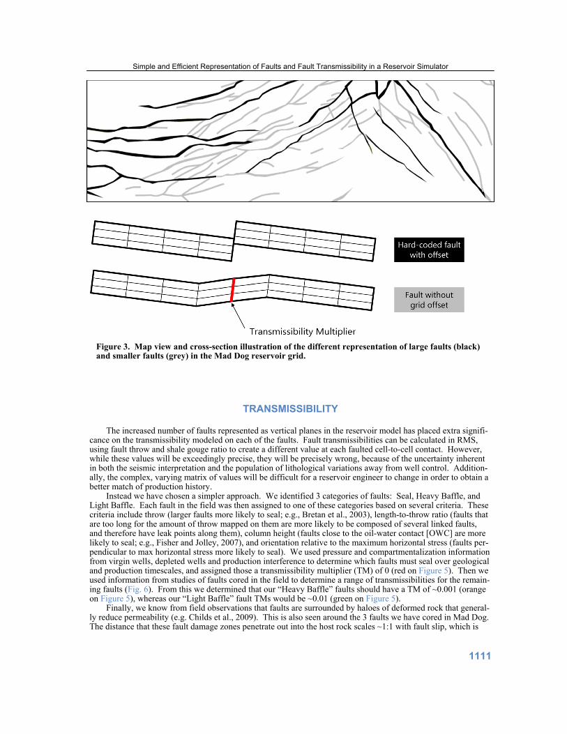
Figure 3. Map view and cross-section illustration of the different representation of large faults (black) and smaller faults (grey) in the Mad Dog reservoir grid.
TRANSMISSIBILITY The increased number of faults represented as vertical planes in the reservoir model has placed extra signifi-
cance on the transmissibility modeled on each of the faults. Fault transmissibilities can be calculated in RMS, using fault throw and shale gouge ratio to create a different value at each faulted cell-to-cell contact. However, while these values will be exceedingly precise, they will be precisely wrong, because of the uncertainty inherent in both the seismic interpretation and the population of lithological variations away from well control. Addition-ally, the complex, varying matrix of values will be difficult for a reservoir engineer to change in order to obtain a better match of production history.
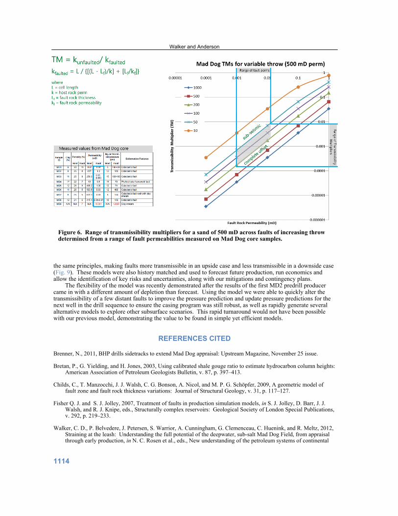
Instead we have chosen a simpler approach. We identified 3 categories of faults: Seal, Heavy Baffle, and Light Baffle. Each fault in the field was then assigned to one of these categories based on several criteria. These criteria include throw (larger faults more likely to seal; e.g., Bretan et al., 2003), length-to-throw ratio (faults that are too long for the amount of throw mapped on them are more likely to be composed of several linked faults, and therefore have leak points along them), column height (faults close to the oil-water contact [OWC] are more likely to seal; e.g., Fisher and Jolley, 2007), and orientation relative to the maximum horizontal stress (faults per-pendicular to max horizontal stress more likely to seal). We used pressure and compartmentalization information from virgin wells, depleted wells and production interference to determine which faults must seal over geological and production timescales, and assigned those a transmissibility multiplier (TM) of 0 (red on Figure 5). Then we used information from studies of faults cored in the field to determine a range of transmissibilities for the remain-ing faults (Fig. 6). From this we determined that our “Heavy Baffle” faults should have a TM of ~0.001 (orange on Figure 5), whereas our “Light Baffle” fault TMs would be ~0.01 (green on Figure 5).
Finally, we know from field observations that faults are surrounded by haloes of deformed rock that general-ly reduce permeability (e.g. Childs et al., 2009). This is also seen around the 3 faults we have cored in Mad Dog. The distance that these fault damage zones penetrate out into the host rock scales ~1:1 with fault slip, which is
1111
difficult to fully implement in a geocellular model with 250 ft long grid cells. Therefore, in addition to the TMs embedded along the fault plane in the model, we reduced the transmissibility of the neighboring grid blocks too, with 0.25 TM in the reference case, and 0.5 and 0.15 in the downside and upside cases respectively.
PRESENCE One of the fundamental, long-standing observations about mapping Mad Dog is that the geophysical map of
the structure does not explain the well pressure and performance data (Walker et al., 2012). We know that there are more features out there than we can see. As our sedimentological evidence and depositional model suggests the reservoirs are somewhat akin to stacked pancakes, the traditional explanation has been that sub-seismic faults are responsible for compartmentalizing the reservoir beyond what we can see. As our image has improved through the years, we’ve been able to identify more faults, and shrink the limits of what is unresolvable. Howev-
Figure 4. Triangle diagram from a representative Mad Dog well log colored by shale gouge ratio, illus-trating that small faults will not allow the DD sand to communicate with the EE/FF sands, and that the EE and FF will likely have poor connectivity across small faults.
Walker and Anderson
1112

Figure 5. Transmissibility multipliers used for Mad Dog reservoir modeling reference case.
er, we cannot accurately resolve faults with less than ~50 ft of throw in the best-imaged areas of the field—and most of the field lies beneath a complex salt body (Walker et al., 2012). From our 30 reservoir penetrations across the field we can estimate that for every fault we can see on seismic, there are at least another 2 faults we cannot see (Fig. 7). Furthermore, our 5 whole cores in the field have unintentionally encountered 3 faults.
We increase our fault density based on these observations, and distribute sub-seismic faults throughout the reservoir model following several principles - small faults should be clustered near big faults, with the roughly the same strike; they may be added where a large fault kinks as a vestigial fault tip (e.g., Fig. 8); added faults should be shorter than the shortest mapped fault; they can link faults that come close but do not otherwise touch; and we will add more faults sub-salt than outboard of salt to honor imaging quality. These added faults are gen-erally modeled as “Light Baffles” using the TM values identified above.
RESULTS
Using this method we have been able to create a reference case Mad Dog reservoir model that is robust yet flexible. After the reference case model was history matched, we created upside and downside realizations using
Simple and Efficient Representation of Faults and Fault Transmissibility in a Reservoir Simulator
1113
the same principles, making faults more transmissible in an upside case and less transmissible in a downside case (Fig. 9). These models were also history matched and used to forecast future production, run economics and allow the identification of key risks and uncertainties, along with our mitigations and contingency plans.
The flexibility of the model was recently demonstrated after the results of the first MD2 predrill producer came in with a different amount of depletion than forecast. Using the model we were able to quickly alter the transmissibility of a few distant faults to improve the pressure prediction and update pressure predictions for the next well in the drill sequence to ensure the casing program was still robust, as well as rapidly generate several alternative models to explore other subsurface scenarios. This rapid turnaround would not have been possible with our previous model, demonstrating the value to be found in simple yet efficient models.
REFERENCES CITED
Brenner, N., 2011, BHP drills sidetracks to extend Mad Dog appraisal: Upstream Magazine, November 25 issue.
Bretan, P., G. Yielding, and H. Jones, 2003, Using calibrated shale gouge ratio to estimate hydrocarbon column heights: American Association of Petroleum Geologists Bulletin, v. 87, p. 397–413.
Childs, C., T. Manzocchi, J. J. Walsh, C. G. Bonson, A. Nicol, and M. P. G. Schöpfer, 2009, A geometric model of fault zone and fault rock thickness variations: Journal of Structural Geology, v. 31, p. 117–127.
Fisher Q. J. and S. J. Jolley, 2007, Treatment of faults in production simulation models, in S. J. Jolley, D. Barr, J. J. Walsh, and R. J. Knipe, eds., Structurally complex reservoirs: Geological Society of London Special Publications, v. 292, p. 219–233.
Walker, C. D., P. Belvedere, J. Petersen, S. Warrior, A. Cunningham, G. Clemenceau, C. Huenink, and R. Meltz, 2012, Straining at the leash: Understanding the full potential of the deepwater, sub-salt Mad Dog Field, from appraisal through early production, in N. C. Rosen et al., eds., New understanding of the petroleum systems of continental
Figure 6. Range of transmissibility multipliers for a sand of 500 mD across faults of increasing throw determined from a range of fault permeabilities measured on Mad Dog core samples.
Walker and Anderson
1114

Figure 7. Example of sub-seismic faulting. A wellbore drilled in the field encounters two seismic faults, both of which can be picked as missing section in the logs. However, detailed dipmeter interpretation reveals an additional 6 faults.
Figure 8. Perspective aerial photograph of a linked fault system from the Volcanic Tablelands, Califor-nia. Vestigial tips, through-going fault, and clustering of small faults near large faults can be seen. Maximum throw on largest fault is ~100 ft. Image is ~3 mi across, with 3x vertical exaggeration. Im-age courtesy of Google Earth.
margins of the world: Proceedings of the 32nd Annual Gulf Coast Section of the Society of Economic Paleontol-ogists and Mineralogists Foundation Bob F. Perkins Research Conference, v. 32, p. 25–64.
Walker, C. D., G. A. Anderson, P. G. Belvedere, A. T. Henning, F. O. Rollins, E. Soza, and S. Warrior, 2015, Compart-mentalization between the GC0738_1 Mad Dog North wellbores—Evidence for post-depositional slumping in the Lower Miocene reservoirs of the deepwater southern Green Canyon, Gulf of Mexico: Gulf Coast Association of Geological Societies Transactions, v. 65, p. 389–402.
Simple and Efficient Representation of Faults and Fault Transmissibility in a Reservoir Simulator
1115

Figure 9. Summary of steps for creating reference case, and upside and downside reservoir models from the seismically-derived map using structural principles.
Walker and Anderson
1116