Embed Size (px)
Citation preview

stingestedst rateles wevola-ple
s
l,
he
DRAFT, PRELIMINARY, COMMENTS ARE APPRECIATED.
Simple Rules in the M1-VECM*
Denise Côté and Jean-Paul Lam
Department of Monetary and Financial AnalysisBank of Canada
234 Wellington StreetOttawa, ON K1A OG9
Canada
[email protected]@bank-banque-canada.ca
June 2001.
Abstract
This paper analyses various simple interest rate rules using a vector error correction forecamodel of the Canadian economy that is anchored by long-run equilibrium relationships suggby economic theory. Dynamic and stochastic simulations are performed using several intererules, including money based rules and their properties are analysed. Among the class of ruconsider in this model, we find that a simple rule with interest rate smoothing minimizes thetility of output, inflation and interest rate. This rule dominates Taylor-type, Ball and other simrules.
*FR-01-002.We would like to thank Scott Hendry, Dinah Maclean, Pierre St-Amant for helpful suggestion
and discussions. Thank you also to Sharon Kozicki our discussant at the CEA 2001 meetings in Montrea
Chris Graham for providing technical help, Jim Day for providing help with the graphs and participants at
the brown bag meeting. The views in this paper are those of the authors and should not be attributed to t
Bank of Canada. All errors and omissions are of our own.

f this
its deci-
us
ing
n-
ifica-
d to
er
ss in
cive in
are
ually
g the
tions.
le has
cta-
ompu-
ness
on.
-
e
s-
1. Introduction
Research on monetary policy rules has exploded in the last few years. Much o
research has focused on finding a simple benchmark rule that the central bank can use in
sion making process. This increased interest in monetary policy rules1, particularly Taylor-type
rules, among academics, central bankers and other researchers, has produced a volumino
amount of information2. In recent years, research on Taylor rules has focused primarily on find
a robust rule that works well across different models3. Uncertainty about the structure of the eco
omy has motivated researchers to try to find a rule that is robust to changes in model spec
tions. These simple rules4, though not optimal, seem to perform better across models compare
more complicated rules which are usually model specific5. Complex rules can be fine-tuned to
account for the specific dynamics of a model but usually perform poorly when tested in oth
models. A simple rule that works well across models, does not only provide more robustne
the face of uncertainty, but is also easier to understand and communicate and is thus condu
establishing and maintaining credibility. However, while it is generally true that simple rules
more robust than complicated rules in the face of uncertainty, not all simple rules perform eq
well. Hence among the class of simple rules, the authorities face the challenge of identifyin
type of rules or class of simple rules which perform well in a wide range of model specifica
The path taken by researchers on finding a robust Taylor-type or other simple interest rate ru
been remarkably similar. Small estimated or calibrated models with or without rational expe
tions and large econometric models with rational expectations are usually used to conduct c
ter simulations. These models vary in level of complexity, details, degree of forward looking
1. Since central banks see themselves as controlling interest rate, this work has attracted a lot of attentiThe usefulness of such type of rule to policymakers however has not been well established.
2. For a comprehensive survey on feedback and Taylor rules, see Armour and Côté (1999).3. The objective of the NBER 1998 conference on Taylor rules was precisely this (Taylor (1999)). Partici
pants were given a set of rules and were asked to perform computer simulations. The Riksbank-IIESAconference in 1998 also looked at interest rate rules in different models. A forthcoming workshop at thBank of Canada in October 2001 will look at Taylor rules in models of the Canadian economy.
4. By simple rule, we mean a rule which is linear and which is a function of only a small number of statevariables.
5. For more details, see Levin, Wieland and Williams (1999). They show that more complex rules are lesrobust to model uncertainty than simpler rules. More complex rules have often to be recalibrated following changes in a model, whereas it is less the case for simpler rules.
Page 2 of 41

ither
e usu-
, in
ls of
1997),
7)
pro-
hould
al
ecent
Can-
ich is
ce
hence
of
con-
uses a
ding
en an
l of
s the
y tod
US
hil-n-
and openness but all are general equilibrium models, have some form of nominal rigidity, e
price and/or wage rigidity and are either dynamic or stochastic in nature. Moreover, rules ar
ally evaluated according to their ability to minimize the variability of key economic variables
particular the inflation rate, output and interest rate.
Most of the studies looking at Taylor-type rules have been conducted on mode
the US economy with few studies done for Canada. Some notable exceptions are Amano (
Atta-Mensah (1998), Armour, Fung and Maclean (2000) and Weymark (2000). Amano (199
estimates a Taylor-type6 rule for Canada for the period 1974 to 1997 and argues that the rule
vides a useful benchmark for comparison with actual movements of the overnight rate but s
not be considered as a viable policy alternative. Atta-Mensah (1998) compares the historic
behaviour of short-term interest rate with a Taylor rule and argues that a such rule explains r
history fairly well. Armour et al (2000) investigates several Taylor-type rules in the Bank of
ada’s Quarterly Projection Model (QPM) and compare them with QPM’s base case rule wh
of an inflation forecast based rule type (IFB). Their results show that Taylor-type rules indu
more variability in output, inflation and interest rates as compared to the base case rule and
do not perform well. However, in the class of Taylor-type rules that minimizes the variability
key economic variables, they recommend a simple Taylor rule with a coefficient of 2 on the
temporaneous inflation gap and 0.5 on the contemporaneous output gap. Weymark (2000)
model à la Svensson (1997) and Woodford (1999)7 and derives efficient classes of rules and the
efficient range for the coefficients on the output and inflation gap for various countries inclu
Canada. She argues that for the period 1983-96, the original Taylor rule would not have be
efficient rule for Canada.8
This paper looks at Taylor, Ball type and other simple rules in a different mode
the Canadian economy which is used to forecast inflation at the Bank. It is in the same spirit a
6. The yield spread and not the overnight rate is used as the instrument.7. These models basically consist of an expectational IS curve and a New Keynesian Phillips curve. The
have reasonable micro foundations and are considered by some as a workhorse model when it comesmonetary policy evaluation. For more details on these models, see Kerr and King (1996), Goodfriend anKing (1997), McCallum and Nelson (1999) and Haldane and Batini (1999).
8. For the six countries she looks at (France, Germany, Canada, Italy, UK, US), she concludes that the was the only country to have implemented an efficient interest-rate policy. However, it seems that herresults may seriously depend on the Lucas type Phillips curve she assumes in the paper. This type of Plips curve may not be appropriate for the countries she looked at and since the original Taylor rule is sesitive to model specification, her results should be interpreted with caution.
Page 3 of 41

mpt to
sim-
ies but
ot
ent
any
of
used
ase
st
d
odel,
ural
ism in
case
., a
ation
do
isas-
nc-d
si-
paper by Armour et al (2000) and can be regarded as part of a series of papers that will atte
find a robust Taylor rule in models of the Canadian economy. Various Taylor type and other
ple rules are explored in the context of a vector error correction model (VECM)9 and the proper-
ties of each rule is assessed. The rules examined in this paper do not exhaust all possibilit
rather are a useful benchmark with which other studies can be compared to.10 We also experiment
with some rules involving a monetary aggregate.11Money supply rules are particularly interesting
in the context of the M1-VECM since the role of money is highlighted in such a model. It will n
only provide an alternative view of the formulation of policy but can also be used to complim
interest rate rules. The objective of this paper is simple. We compare the performance of m
simple interest rate rules with the existing reaction function in the VECM. Among the class
simple rules, we also identify which one works reasonably well and hence can possibly be
for policy advice.
We find that in general, the Taylor rule does not perform as well as the base c
reaction function12 since it induces more variability in output, inflation and especially in intere
rates. A possible intuition behind this result is as follows: by considering only the output an
inflation gap when setting interest rates, the Taylor rule ignores important features of the m
in particular the money gap. Unlike in many other models, the money gap affects the struct
equations of the model and since money plays an important role in the transmission mechan
this model, it is not surprising to see that the Taylor rule does not perform as well as the base
rule. However, in the class of Taylor-type rules, we tend to find that the original Taylor rule i.e
rule with a coefficient of 0.5 on the contemporaneous output gap and contemporaneous infl
gap, performs reasonably well.13 Our findings also tend to show that the Ball and change rules
9. For a detailed exposition about the M1-VECM, see Hendry(1995), Adam and Hendry((1998).10. There are certainly other combinations that will perform better. The objective of this paper is not only to
see if a Taylor rule would work well in the M1-VECM but also to find a robust rule that can be used inother models of the Canadian economy.
11. The performance of money supply rules may be better than interest rate rules especially when inflationhigh and volatile. In such circumstances, inflationary expectations and the output gap are harder to meure and hence this reduces the usefulness of interest rate rules.
12. We sometimes refer to the base case reaction function as the base case rule. The existing reaction fution in the VECM is estimated over history and is not a rule in the strict sense. However, we can regarsuch reaction function as representing an unconstrained rule.
13. We also find a similar result when we consider rules involving the yield spread, not the overnight rate, athe instrument. In some cases we investigated, rules using the yield spread slightly outperform the orignal Taylor rule.
Page 4 of 41
y sur-
g the
nd
per-
rules
ase
ting
2000).
e lit-
the
ncor-
simi-
e
s.
he
ese
e
not perform as well as simple Taylor rules. This may largely be explained by the uncertaint
rounding the calculation of the equilibrium exchange rate.14 Because of the added uncertainty
about the equilibrium exchange rate and since it performs poorly, we do not recommend usin
Ball rule in this context.
We also find that a rule involving the growth rate of money performs relatively
well compared to the Taylor rule but is inferior to a rule with smoothing. Like Clarida, Gali a
Gertler (2000) and Levin et al (1999), we find that rules with interest rate smoothing tend to
form relatively well compared to the base case rule and other simple rules. In some cases,
with smoothing, significantly reduce the variability of interest rates without inducing any incre
in the volatility of output and/or inflation. The smoothing parameter was obtained by estima
some reaction functions for Canada using the same method as in Clarida, Gali and Gertler (
The paper is organized as follows. Section 2 offers a very brief overview of th
erature on Taylor type rules and motivates our paper. Section 3 gives a short description of
M1-VECM, some of the shocks we consider. Section 4 explains how Taylor type rules are i
porated in the VECM. Section 5 describes how Taylor-type rules behave in the model when
lar shocks are considered and presents our results, section 6 presents our results from som
stochastic simulations performed using the “best” set of rules and section 7 finally conclude
2. Literature review
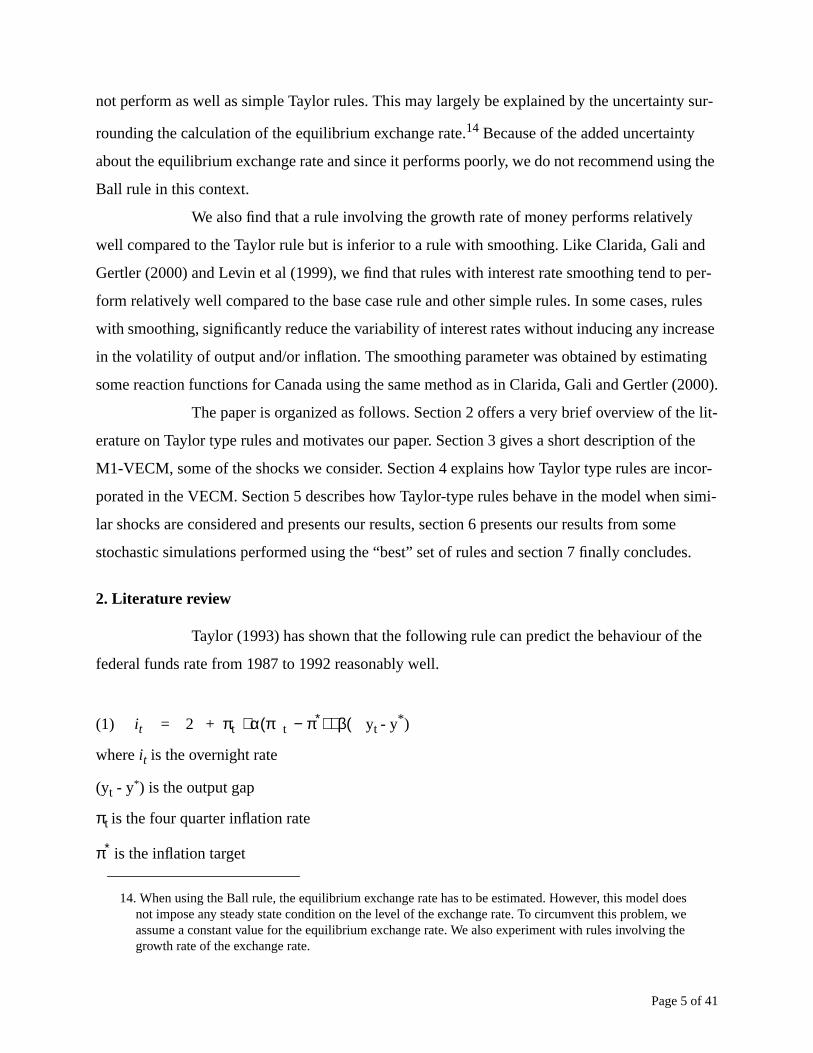
Taylor (1993) has shown that the following rule can predict the behaviour of t
federal funds rate from 1987 to 1992 reasonably well.
(1) it = 2 + πt + α(πt − π∗) + β(yt - y*)
whereit is the overnight rate
(yt - y*) is the output gap
πt is the four quarter inflation rate
π∗ is the inflation target
14. When using the Ball rule, the equilibrium exchange rate has to be estimated. However, this model donot impose any steady state condition on the level of the exchange rate. To circumvent this problem, wassume a constant value for the equilibrium exchange rate. We also experiment with rules involving thgrowth rate of the exchange rate.
Page 5 of 41

ous
osed
cross
l
pora-
e Tay-
f
l infor-
g a
coun-
riety
many
e of
ule
n rate
f thetan-lort
r
so
According to the Taylor rule, the overnight rate responds to the contemporane
deviation of inflation from its target and to the contemporaneous output gap.15Taylor assumes a
long run equilibrium value of 2 for the real interest rate and a constant weight of 0.5 was imp
on both gaps.16 This simple rule which has been modified in a number of ways, continues to
attract a lot of attention and has performed reasonably well in a wide variety of models and a
countries.
The inflation and output gap term reflects some of the objectives of the centra
bank which is low and stable inflation and promoting sustainable output growth. The contem
neous output gap term is also often regarded as bringing a forward looking dimension to th
lor rule since it is viewed as capturing future increases in inflation. This view relies heavily o
course on the assumption that the measure of the output gap is reliable and has substantia
mation content on future inflation, an assumption which can be weak.
In recent years, research on Taylor rules have focused more heavily on findin
rule which can be used across a wide range of models and which can be applied to different
tries. There is now more evidence that simple rules like Taylor’s perform better in a wide va
of models than more complex rules and are also robust across countries.17 For example Levin et al
(1999), using four different structural macroeconomic models18, find that simple rules are more
robust to model changes than more complicated rules. The four models used are different in
respects in terms of level of aggregation, specification of output and price dynamics, degre
openness and forward lookingness and estimation technique and period. They find that a r
which reacts to the current output gap, the one to three year moving average of the inflatio
15. McCallum (1999) has argued that such type of rules may not be operationally feasible as the inflationand output gap are usually not known at the time the authorities have to set interest rates. This type ooperationality issue has also been emphasized by Orphanides (1997). Orphanides (1997) argues thatcurrent period values for the output gap are not observed and are usually subject to frequent and substial revisions after they are initially reported. He argues that these problems are so severe that the Tayrule would not have prevented the inflation of the 1970s as claimed by Taylor if revised data on the outpugap is used. We experimented with a more “operational” Taylor rule by including the lagged values of theoutput and inflation gap instead of their contemporaneous values but found it made little difference to ouresults.
16. Taylor (1993) deduced his rule from the observed behaviour of the FOMC. However, such rule can albe derived from a simple IS-PC model.
17. Although results on the robustness of the Taylor rule come mostly from closed economy models withsimilar framework.
18. The four models used are Fuhrer and Moore model, Taylor’s Multi-Country Model, The FRB Staffmodel and the MSR model of Orphanides and Wieland.
Page 6 of 41

dels
ult is
c
s or
high
rules
sev-
e
tion of
999)
s that
ooth-
ce for
gged
e
gap,
ously,
rule
most
rect.
esults
99)
ons
9).ddc-
oci-
and which contains a high degree of interest rate smoothing performs very well in all four mo
while more complicated rules perform much worse when tested in all four models. This res
rather intuitive as more complicated rules are generally fine-tuned to account for the specifi
dynamics of a model and when tested out, they are likely to perform poorly as the dynamic
specifications of different models are not the same. They also show that a simple rule with a
degree of smoothing outperforms both the original Taylor rule and inflation forecast based
and is more robust to model changes.
The conference on monetary policy rules held at the NBER in 1998 also tested
eral simple rules in nine different models.19 The findings from this conference tend to confirm th
robustness of simple rules, although there are disagreements about the type and specifica
the simple rule. For example, Haldane and Batini (1999) and Rudebusch and Svensson (1
find that forecast based rules are preferred to the simple Taylor-type rule. Ball (1999) argue
an MCI based rule is preferred to the simple Taylor rule and a rule with some interest rate sm
ing. He also shows that rules with interest rate smoothing not only generated a higher varian
output and inflation but also for interest rates.20 On the other hand, Rotemberg and Woodford
(1999) propose a rule with a small weight on the output gap and a very high weight on the la
interest rate.
When dealing with Taylor rules, there are other type of uncertainties which ar
often ignored. The Taylor rule is made up of four components: the output gap, the inflation
the equilibrium interest rate and the weights assigned to the two gaps. As mentioned previ
there is a lot of uncertainty surrounding the output gap and how it is calculated. Moreover, the
assumes a constant value for the equilibrium interest rate. The equilibrium interest rate will
likely fluctuate in response to real disturbances and assuming a constant value may be incor21
There is also some uncertainty about which measure of inflation to use. For example, the r
may be sensitive to whether total CPI or any other measure of inflation is used. Kozicki (19
presents evidence on how these Taylor type rules may not be robust when some assumpti
19. The participants were given 5 different rules to test in their models. For more details, see Taylor (19920. Ball’s results should be interpreted with caution as his model is a backward looking model. In backwar
looking models, the expectational channel is shut off, hence movements in short-term rates usually leato substantial changes in the long-term rate and hence real output. As a result, efficient policy is charaterized by very little persistence in interest rates.
21.Estimates of the equilibrium interest rate may also not be reliable and share some of the problems assated with estimating the output gap.
Page 7 of 41

ow the
used.
inty is
ky
cy
ave an
pas-
the
of the
d in
hich
smis-
1,
nd for
s the
ges in
y
t on
e
-nnt
e
about the rule are altered. She argues that policy recommendations can vary depending on h
output gap is measured and which measures of the equilibrium interest rate and inflation are
We do not address many of these issues in this paper but are aware that this type of uncerta
important.
3. A Brief Description of the M1-VECM
The model which is used in this paper is very different from the traditional stic
price-’intertemporal IS’ model usually used to analyse interest rate rules and monetary poli
questions. Most of the models used to evaluate the robustness of Taylor type rules do not h
explicit role for money22. In these models, the money supply is endogenous and money has a
sive role (the monetary authority simply has to supply the right amount of money to achieve
desired level of interest rate.) Moreover, since changes in money growth do not enter in any
structural equations23 and hence do not feed back into the model, money can often be ignore
these models. In this paper, we investigate the performance of Taylor type rules in a model w
has at its heart a long-run money demand function and where the role of money in the tran
sion mechanism is highlighted.24 The M1-VECM estimates a long-run relationship between M
prices, output and short-term interest rate and this vector is regarded as the long-run dema
money. In this model, even with an interest rate rule, money does not play a passive role. A
money supply has to change to achieve the desired level of interest rate, this leads to chan
the money gap, the difference between actual money supply and estimated long-run mone
demand, and since the money gap feeds into the output and price equation, it has an effec
these variables.
22. Models with an IS curve, a Phillips curve and an interest rate rule often ignore the LM curve. In thesemodels, once the interest rate is determined, the LM curve only tells us the amount of money that must bsupplied to achieve the desired level of interest rate and hence is residually determined.
23. For money to have a role in these sticky price IS-LM models with a Taylor type interest rate rule, a monetary aggregate can be included in the IS function for example. McCallum (2001) derives such a functiobut shows that the inclusion of a monetary aggregate in such a framework is not quantitatively importaand can therefore be excluded. The same conclusion is reached by Ireland (2000).
24. The long-run equilibrium relationships in the model are combined with a short-run dynamic structure onwhich much uncertainty lies. Money, in particular the money gap feeds into the structural equations of thmodel.
Page 8 of 41

-
licy
e dif-
n is
tion
ss
ndry
ply
que
t rate.
y
that
help
viour
ed by
ing
t-run
each
tem
, infla-
The M1-based vector-error-correction model (M1-VECM), which currently pro
vides the analytical background against which the Monetary and Financial Department’s po
recommendations are designed, is a model which gives a primary role to the money gap, th
ference between money demand and supply. In most large scale economic models, inflatio
largely driven by the level of excess demand in the goods and labour market and since infla
growth depends on excess demand, usually through a Phillips curve relationship, this exce
demand causes inflation. Unlike these models, the M1-VECM model, first developed by He
(1995), uses an active-money paradigm in which disequilibrium between actual money sup
and estimated long-run money demand, called the money gap, causes inflation.
Using the Johansen-Juselius (1990) methodology, the model estimates a uni
and stable long-run cointegrating vector between M1, CPI, real GDP and short-term interes
This relationship is interpreted as the long-run money demand function. The long-run mone
demand function is then used to calculate the money gap. Adams and Hendry (1999) show
the money gap has moved very closely with inflation over the last forty years and hence may
to predict inflation. In this model, the cointegrating vectors determine the steady-state beha
of the variables while the dynamic response of the main variables of the model is determin
the VAR portion. This model can be regarded as addressing the classic problem of combin
long-run equilibrium relationships on which one has a high degree of confidence with a shor
dynamic structure on which much uncertainty lies.
The model has four main forecasting equations and the money gap enters in
of these equation, indicating the role money plays in this framework. The reduced-form sys
represented below defines the main macroeconomic linkages that determine money growth
tion, output growth and the change in overnight rate.
∆M1t
∆CPIt∆Yt
∆Rt
Γ L( )
∆M1t
∆CPIt∆Yt
∆Rt
αM1
αCPI
αY
αR
MGAPt 1– ΘtZt+ +=
Page 9 of 41

e
tion,
ocks.
or US
it by a
dies
tes are
ules
used
ules
it was
stly
ase
deter-
e are
eed at
enc-
eventu-
omy
stru-
e
where G(L) is a matrix of fourth-order lag operator, MGAPt-1 is the money gap derived using th
long-run money demand function and Zt is a matrix of predetermined and dummy variables.25
The model is then estimated with some equilibrium conditions imposed on output, infla
money growth and the overnight rate.
In this paper, the model and the various rules are analysed under different sh
We assume that the economy can be hit by a demand, nominal exchange rate, money
interest rate shock. Except for the US interest rate shock, we assume that the economy is h
one percent shock in period 126 and this shock declines by a factor of 0.25% each quarter and
out after four quarters. In the case of a US interest rate shock, we assume that interest ra
reduced by 25 basis points for four quarters starting in period 1.
4. Simple Rules in the M1-VECM
We investigate several simple interest rate rules in the model. These simple r
are imposed only over the forecast or projection period while the existing base case rule is
over the historical period. The rationale behind this is simple. When some of these simple r
were imposed over history, the model had some problems converging to its steady state and
decided to use these rules only over the projection period. More importantly, as we are mo
interested in comparing the performance of simple rules with each other and the existing b
case rule, it is not unreasonable to impose the new rule only over the forecasting period and
mine whether or not it would be optimal to use such type of rules. The properties of each rul
assessed in terms of the resulting variability of output, inflation and interest rates and the sp
which the economy returns to its steady state. The latter will not play a significant role in influ
ing our results as these simple rules are imposed in such manner to ensure that the model
ally converge to its steady state.
As already mentioned, we look at many different type of rules, e.g open econ
rules, generalized Taylor rules or rules with smoothing, rules with the yield spread as the in
25.Please note that this is a very raw representation of the M1-VECM. For a more accurate description of thactual model, see Adams and Hendry (1999).
26. Our simulations with the shocks start in the last quarter of 2000.
Page 10 of 41

oney
nt to
les
and
expo-
h other
that
e rate
es
rate
to the
ces
lated.
hange
e
ge
rules,
oved
ut-d
ment, rules with more than one lag of the output and inflation gap and rules containing the m
growth rate. Some of these rules have performed well in one or many models. Since we wa
compare our results with other studies, the coefficients selected for the different types of ru
were of similar magnitude. In addition, we also investigate many other different combinations
those which were inferior to the benchmark rule were rejected. For ease of comparison and
sition, the “best” rule in each category is selected and these rules are then compared to eac
and to the base case reaction function.
Open economy rules are motivated by the findings of Ball(1999) who argues
the simple Taylor rule should be modified in open economy models to account for exchang
effects. According to Ball (1999) adding the exchange rate to the original Taylor rule improv
macroeconomic performance in small open economy models.27 In our case, we look at several
types of open economy rules. In the first case, we look at the Ball rule where the exchange
gap, i.e. the difference between the actual exchange rate and the equilibrium rate, is added
benchmark rule. The Ball rule is given by
(2)
whereπt is core inflation
et is the nominal exchange rate
is the equilibrium exchange rate
In addition to the uncertainty surrounding the output gap, the Ball rule introdu
other uncertainties. When using the Ball rule, the equilibrium exchange rate has to be calcu
As the M1-VECM model does not have a steady state or equilibrium level for the nominal
exchange rate, we have to make some assumptions about the equilibrium value of the exc
rate. As in Armour et al (2000), we assume a constant value for the steady state value of th
exchange rate throughout our exercise.28 Moreover, since we do not know the degree of exchan
rate pass- through, we investigate with two measures of inflation when using open economy
core inflation and core-core inflation, i.e., direct exchange rate pass-through effects are rem
27. Ball (1999) argues that the inclusion of the exchange rate as a policy variable in his model, reduces oput variability by around 17% for the same amount of inflation variability. Since most models are closeeconomy models, the robustness of such results needs further checking.
i t i α πt
π–( ) β yt
γ et e–( )+ + +=
e
Page 11 of 41

)
es.
e
e in the
e rate
ding
cted
ut
and
inter-
ooth
at the
ooth-
999)
sig-
vesti-
in
i-n
ng
from core inflation. To construct our core-core inflation series, we follow Armour et al (200029
and subtract a weighted average of ten lags of the exchange rate from the level of core pric
Because of the above uncertainties, the Ball rule is often avoided.30
We also look at another open economy rule which is similar to the Ball rule, th
change rule. When the change rule is used, the exchange rate gap is replaced by the chang
exchange rate and the equilibrium exchange rate need not be estimated.
The change rule is given by
(3)
To ensure that the model converges, we assume that any gap in the exchang
disappears after fifty years. While the change rule avoids some of the uncertainties surroun
the Ball rule, it has the drawback of not being formally derived from a model. We also condu
some experiments with rules containing the change in the rate of growth of the exchange b
found that these rules perform poorly.
We also investigate rules with interest rate smoothing as in Clarida et al (2000)
Levin et al (1999). According to them, it is common practice among central banks to adjust
est rates only gradually and the desired level is usually achieved after several small and sm
changes. Clarida et al (2000) estimate reaction functions for different countries and show th
coefficient on the lagged interest rate is relatively high, indicating a very high degree of sm
ing. When rules with interest rate smoothing are introduced in the four models Levin et al (1
consider in their study, they show that the volatility of output, inflation and interest rate was
nificantly reduced. They argue that from the numerous permutations of simple rules they in
gate, rules with a high degree of smoothing provide the most significant gains.
Interest rate smoothing rules are given by
28. A constant value for the equilibrium exchange rate is a gross oversimplification of the real world and the case of Canada, this is very unrealistic. We are fully aware of this limitation and this is why the resultsfor the Ball rule should be treated with caution. We experiment with several different values for the equlibrium exchange rate. In almost all cases, the Ball rule performs very poorly and should not be used ithis model.
29. For more details, see page10 in Armour et al (2000).30.Even when these uncertainties are partially accounted for, many studies do not find any gain from usi
the Ball rule over the Taylor rule even in an open economy model.
i t i α πt π–( ) β yt γ et et– 1–( )+ + +=
Page 12 of 41

mon
ment
ually
icy
ous
with
and
djust-
not
rest
gap.
f the
inter-
f long-
cen-
ntral
r about
rest
(4a) it = ρit-1 + (1 − ρ)it∗∗
(4b) it∗∗ = α(πt − π∗) + β(yt - y*) + i∗
Combining (4a) and (4b), we get equation 4
(4) it = ρit-1 + (1 − ρ)α(πt − π∗) + (1 − ρ)β(yt - y*) + (1 − ρ)i∗
There are several reasons to explain why interest rate smoothing may be com
practice among central bankers.31 With smoothing, large volatility in interest rates can often be
avoided, therefore minimizing disruptions in the financial markets. It may also reflect an ele
of prudence on the part of central bankers. Moreover, frequent reversals in interest rates us
undermine the credibility of a central bank and are usually avoided. More importantly, a pol
rule which contains a lagged interest rate, implicitly responds not only to the contemporane
output and inflation gap but also to lagged output and the inflation gap. In other words, a rule
interest rate smoothing provides some measure of the historical behaviour of the economy
thus incorporates more information about the economy. Hence, instead of reflecting partial a
ment, the lagged interest rate term may be evidence of persistent special factors or events
properly accounted for in the rule. This is interesting in the context of this model. Lagged inte
rates may not only contain information on lagged output and inflation but also on the money
Thus a rule with inertia or smoothing implicitly takes into account the information content o
money gap. This is a possible reason why this type of rule works well in this model.
Moreover, Goodfriend (1991) has argued that smooth changes in short-term
est rates provide greater control over long-term interest rates. This is important especially i
term rates play an important role in economic decisions. By controlling the long-term rate, a
tral bank can thus have a better control on output and inflation. If such is the case, then ce
banks engage in smoothing not because they care about short-term interest rates but rathe
having greater control on output and inflation.
Recently Woodford (1999) has put forward another reason why rules with inte
rate smoothing perform well in forward looking models.32 According to Woodford (1999), inter-
31. See Sack and Wieland (1999) for example.
Page 13 of 41

ing
ent,
nt is
elp
preci-
n
at
infla-
ut
istent
t
ida et
factor
form-
Clar-
s
tar-
e
al
y-
e
est rate smoothing rules can help a central bank improve its performance when it is operat
under discretion. Woodford (1999) shows that when a central bank is acting under commitm
the optimal outcome displays a large degree of policy inertia. Since policy under commitme
not realistically feasible33, a rule that displays a large degree of inertia under discretion can h
the central bank move closer to the commitment outcome. This argument can be better ap
ated with the following example. In an economy with forward looking agents, current inflatio
depends also on expected inflation. Suppose the economy is hit by an inflationary shock th
requires a contractionary monetary policy. If the contraction is expected to persist, expected
tion will fall and this will in turn reduce current inflation, improving the trade-off between outp
and inflation. Hence a given reduction in inflation can be achieved at a smaller but more pers
reduction in the output gap.
When rules with smoothing are used, Taylor’s original coefficients are kept bu
they are adjusted accordingly to reflect the degree of interest rate smoothing. We follow Clar
al (2000) and assume that the coefficients on the output and inflation gap are adjusted by a
of (1-ρ) whereρ is the degree of smoothing. The smoothing parameter was obtained by per
ing some GMM estimation for the period 1980 to 1999 using the same method advocated by
ida et al (2000).
The literature on simple rules has paid very little attention to money based
rules. In fact, rules which give a prominent role to money have become a rarity in economic
and advocates of a monetary based rule are rare. Some notable exceptions are McCallum
(2000) and Meltzer (1999). The disappearance of money as an instrument or intermediate
get is mostly due to the perceived instability of money demand and also to new views on th
transmission mechanism. Moreover, as compared to a money based rule, the Taylor rule is
much more attractive since it is expressed in terms of the instrument actually used by centr
banks. Recent empirical evidence on the performance of money based rules is also rare.
McCallum (2000) compares the historical performance of a monetary based rule with the Ta
lor rule for Japan, the UK and the US. He shows that in a number of cases, especially for
32. Although the M1-VECM is not a forward looking model, the money gap can be regarded as providinginformation about future inflation.
33. Policy under commitment is not time consistent. A central bank always has the incentive to renege oncthe effects of a shock have dissipated.
Page 14 of 41
the
g
rt
More-
se as
sed by
l
gap
econ-
s is
ene
Japan, a money based rule would have given better recommendations to policymakers than
Taylor rule. Despite this claim, McCallum’s rule has still not attracted a lot of attention.34
Since money has an important role in this model, we look at rules involving the
change in the growth rate of adjusted M1. We experiment with such rules by allowingβ to take on
different values,λ to be 0.5 andα to be 1.5 in equation (6). This rule with money growth targetin
can be regarded as a hybrid rule of Taylor’s (1993) and McCallum’s (2000).
(6) it = i∗ + α(πt − π∗) + λ(yt - y*) + β(∆Mt - ∆M*)
where∆Mt is the growth rate of adjusted M1 and∆M*is the target for the growth rate of adjusted
M1.
We also tested rules involving different weights forλ, β andα. For example, we
experimented with a rule involving only the money growth term, hence settingα andλ to be zero
in equation (6). We also tested a rule withλ set to zero andα andβ taking on different values.
Note that for stability reasons, the weight onβ was restricted to be less than 0.75. We only repo
the results for some of the combination of rules we tried in the model. We also tested a rule
involving the money gap. However, the model did not converge when such a rule was used.
over, we do not experiment with a purely money based rule, i:e., a rule with the monetary ba
the instrument and not the interest rates, as the monetary base is not the actual instrument u
central banks and is thus not realistic.
Finally, we also experimented with other types of rules. These include nomina
income targeting rules, rules containing more than one lag of either the output or the inflation
and rules with the yield spread as the instrument. These rules were restricted to be closed
omy rules. In general, these rules did nor perform as well as the original Taylor rule and thi
why we do not report any of these results.
34.McCallum (1999) argues that policymakers “view discussions of the monetary base with about the samenthusiasm as somebody would have for the prospect of being locked in a telephone booth with someowho had a bad cold or some other infectious disease.”
Page 15 of 41

ic
lor
e
well
the
output
.
at in
at out-
rule
esults
r rate
rates
n to
m his-
uce
pris-
he
cases
e
n the
ra-
the
5. Our Results.
To compare the different rules, we look at the variability of all key macroeconom
variables, especially at output, inflation and interest rates. We first compare the original Tay
rule with other Taylor type rules with different coefficients on the output and inflation gap. W
find that the original Taylor rule, with a coefficient of 0.5 on both gaps performs reasonably
compared to other Taylor-type rules.35 As seen in Figure 1, when hit with a demand shock the
original Taylor rule induces a slightly lower volatility of output and inflation and much lower
interest rate volatility compared to the other Taylor-type rules. This result is also robust for
various shocks we consider. Moreover, rules with a coefficient greater than 2 on either the
or inflation gap tend to perform very poorly and are even unstable in certain circumstances
When the original Taylor rule is compared to the base case rule, we can see th
general it does not perform as well. For example, in the case of demand shocks, it is seen th
put deviates more from its target under the original Taylor Rule compared to the base case
and interest rates are much more volatile under the original Taylor rule. We obtain similar r
for the other shocks. However, under the Taylor rule, inflation returns to its target at a faste
compared to the base case. This can be explained to some extent by the fact that interest
move more aggressively under a Taylor rule, as seen by its higher volatility, and force inflatio
move back to its target at a faster rate. Moreover, since the base case rule is estimated fro
tory, it is not surprising that it has a slower path to equilibrium than the original Taylor rule.36
When the weight on the output gap is increased, it is seen that it does not red
the deviation of output from its target nor does it reduce the volatility of output. This is a sur
ing result to some extent, as one would expect output to deviate less from its target when t
weight on the output gap is increased. This counter intuitive result is also obtained in some
when other rules are used and when stochastic simulations are performed on the model.
Our findings are different from Armour et al (2000). They recommend a simpl
rule with a coefficient of 2 on the inflation gap and 0.5 on the output gap and argue that withi
35. We do not report results of rules which use the lagged output and inflation gap and not the contemponeous gap. The results were not very different from the original Taylor rule or were marginally worse insome cases.
36. The base case reaction function also contains many more lags of the output gap and interest rate thanoriginal Taylor rule and hence displays more inertia.
Page 16 of 41

k to
it is
ithout
rly
del
es the
sults
e
ugh
asy to
ompa-
oeffi-
d to
e.
ys:
s on
ltered
are
of the
ce it
Ball
were
ht
s-
context of QPM, the original Taylor rule does not work well as it does not bring inflation bac
its target quickly enough. When their recommended Taylor rule is introduced in this model,
seen in Figure 2 that it induces more variability in output and especially on interest rates w
any noticeable reduction in the variability of inflation. The QPM-Taylor rule performs very poo
in this model and hence offers further evidence on how sensitive simple rules can be to mo
specifications.
We find similar results when rules with the yield spread (thereafter YS rule)
instead of the overnight rate as instrument are investigated. We find that a YS rule which us
same coefficients as the original Taylor rule performs well and in many cases, gives similar re
as the original Taylor rule. This rule even slightly outperforms the original Taylor rule in som
cases since output and especially interest rates are less volatile. This small gain is not eno
however to outweigh some of the other benefits a simple Taylor rule can bring, e.g being e
communicate and understand. Moreover, since we want to find a rule which is robust and c
rable across models37, we do not opt for a YS rule.38. As it is the case for the original Taylor rule,
we find that in the class of YS rule, a coefficient of 0.5 on both gaps is warranted. Higher c
cients on both gaps usually result in higher variability in interest rates, output and inflation an
outright instability in some cases.
To a large extent, our results are similar to Armour et al (2000) on the Ball rul
The Ball rule does not perform well in this model. We experiment with the Ball rule in two wa
first we keep the coefficient on the exchange rate gap fixed at 0.25 and alter the coefficient
both the output and inflation gap and second, the coefficient on the exchange rate gap is a
while the coefficients of the original Taylor rule are used for the output and inflation gap and
kept fixed. When the coefficient on the exchange rate gap is allowed to change while those
output gap and inflation gap are kept fixed, we find that the Ball rule performs very poorly sin
induces excessive volatility in output, inflation and interest rates. As shown in Figure 3, the
rule induces secondary cycling in output and wide fluctuations in interest rates. The results
not substantially different when we experimented with different values for the equilibrium
37. To our knowledge, other studies have not considered rules containing the yield spread as the overnigrate is often seen as the instrument a central bank can directly control.
38. There are of course, other practical difficulties associated with a rule involving the yield spread such abeing operationally feasible. There is also greater uncertainty surrounding the calculation of the equilibrium yield spread.
Page 17 of 41

is rule
fi-
the
we
ub-
rule is
some
e of
reduce
ince it
m
Ball
ell
ive sec-
to
poor
ed
ely
ee of
vola-
te. It is
ee of
en
nder
hile
exchange rate. The verdict on the Ball rule is not very different when the coefficient on the
exchange rate gap is fixed while the other coefficients are altered. As shown in Figure 4, th
induces more output volatility, although in this case, there is no secondary cycling but signi
cantly more volatility in interest rates. We also obtain poor results when different values for
equilibrium exchange rate were used.
Since the Ball rule explicitly takes into considerations the exchange rate gap,
should expect it to perform well compared to the original Taylor rule when the economy is s
jected to exchange rate shocks. However, the results indicate that in this case also, the Ball
still dominated by the Taylor rule and is thus not recommended. We have already discussed
of the practical issues which can arise when using such type of rules. The poor performanc
Ball type rules can be attributed to some extent to these factors. If such is the case and to
this type of uncertainty, it is recommended to put a zero weight on the exchange rate gap. S
performs poorly and because of the uncertainty surrounding the calculation of the equilibriu
exchange rate, we do not recommend using the Ball rule in this context.
The change rule does not perform well in this model also. In many cases, the
results from this type of rules are either marginally or noticeably worse as compared to the
rule. Rules involving the change in the rate of growth of the exchange rate do not perform w
also. In general, they induce more output and interest rate volatility (in some cases excess
ondary cycling) without any reduction in the variability of inflation. Hence, our findings tend
show that open economy rules do not work well in this model. Some of the reasons for this
performance have already been provided.
Like Levin et al (1999), we find that rules with smoothing perform well compar
to the original Taylor rule and other simple rules. As previously mentioned, we use a relativ
high value for the smoothing parameter. Figure 5 shows how different rules with various degr
smoothing perform when the economy is hit with a demand shock. As is clearly shown, the
tility of output and interest rates is reduced as the weight increases on the lagged interest ra
interesting to note that while the variability of output and inflation is reduced when the degr
smoothing is increased, the volatility of inflation is virtually unchanged. Furthermore, it is se
that a rule with a high degree of inertia performs relatively well compared to the base case. U
this type of rule and with a demand shock, it is seen that output volatility is slightly higher w
Page 18 of 41

ilar
in
m-
tly
thing
ll in
e
lity,
tries. If
ocu-
nter-
my. If
h
s
er var-
y in a
hen a
make
is
wed
rowth
ut and
ses,
oney
ith a
as
interest
oney
interest rates volatility is lower and inflation returns to target at a faster rate. We obtain sim
results for other shocks, indicating that this rule is also robust across shocks.
When this rule is compared to the original Taylor rule and the Ball rule, it is seen
Figure 6 that following a demand shock, the volatility of output is lower under such a rule co
pared to the original Taylor and the Ball rules, while the volatility of interest rates is significan
reduced. In the case of an exchange rate, money and foreign rate shocks, a rule with smoo
also outperforms the other simple rules. In short, rules with smoothing work remarkably we
this model and outperform any other simple rule we investigated.
It is interesting to note that as in Levin et al (1999) and Clarida et al (2000), w
also find that such rule can lead to gains in terms of output, inflation and interest rate volati
indicating that such rule are not only robust across models and shocks but also across coun
such rules are effectively a good characterization of monetary policy in many countries as d
mented by many, it is not surprising that it performs well in this model. Hence, it would be i
esting to see if such a rule would also perform well in other models of the Canadian econo
such is the case, it would provide further evidence about the robustness of simple rules wit
smoothing. We have already given some reasons why such types of rules may work well. A
argued before, lagged interest rate may serve as a proxy for lagged output, inflation and oth
iables in the economy. As a result, this rule incorporates more information about the econom
sub optimal way and thereby offers policymakers greater control on output and inflation.
Figures 7, 8 and 8a, show the response of output, interest rates and inflation w
money based rule is used. The three different graphs refer to three different assumptions we
regardingλ, β andα in equation (6). Figure 7 refers to the case where a money growth term
added to the original Taylor rule and where only the weight on the money growth term is allo
to change. In Figure 8, the weight on the output gap is set to zero while that on the money g
term is allowed to change. Figure 8a refers to the case where the weights on both the outp
inflation gap are set to zero while that on the money growth term is allowed to vary. In all ca
the weight on the money growth term does not exceed 0.75 for stability reasons. When the m
growth term is added to the original Taylor rule, as shown by Figure 7, it is seen that a rule w
weight of 0.25 on the money growth term dominates the other two money rules. Moreover,
compared to the basecase reaction function, output deviates more from its steady state and
rates are much more volatile. As compared to the original Taylor rule, the addition of the m
Page 19 of 41

volatil-
ero.
it
ced.
sting
ion of
ilar
that
ady
arable in
nly
nder
the
rule
e
more
ith
ared
ule
e dif-
el,
based
.8 and
Taylor
as set
growth term does not lead to any improvements. On the contrary, it seems to induce more
ity in output and in interest rates.
Figure 8 shows a similar rule but where the weight on the output gap is set to z
When this type of rule is compared to the other money based rule (Figure 7), it is seen that
slightly outperforms the latter. The volatility of output, interest rates and inflation are all redu
There is especially a marked difference in the volatility of interest rates. This result is intere
since it shows that in such a model, a rule which contains the money growth rate, the deviat
inflation from its target and the commonly used output gap would be outperformed by a sim
rule which excludes the output gap. If the rule contains only the money growth term, it is seen
it performs slightly better than the two other money based rules. Output deviations from ste
state under such a rule are less as compared to the rules in Figures 7 and 8 and are comp
magnitude to the rule with a high degree of smoothing (Figure 5). Since interest rates are o
reacting to the deviations of the growth rate of money from its target, the interest rate profile u
such a rule is very different from the other rules we tested in this model.
Figure 9 compares the “best” money growth rule with the rule with smoothing,
Taylor rule and the basecase reaction function. As mentioned previously, the money growth
performs relatively well when it comes to output stabilization, slightly outperforming both th
Taylor and the rule with smoothing. On the other hand, inflation under such a rule deviates
from its target and for a longer period of time as compared to the Taylor rule and the rule w
smoothing. Moreover, the money growth rule induces more volatility in interest rates as comp
to the rule with smoothing but substantially less volatility than the Taylor rule. Overall, the r
with smoothing seems to outperform both the Taylor rule and the money growth rule but th
ference between all three rules are not large
6. Stochastic simulations.
Once we have identified which types of rule work reasonably well in this mod
some stochastic simulations were performed using the Taylor-type rule, the money growth
rule and the rule with smoothing. For the latter case, the smoothing parameter was set at 0
0.9. The parameter on the output gap was set successively at 0, 0.25, 0.5, 1 and 1.5 for the
rule and the rule with smoothing. For the money based rule, the weight on the output gap w
Page 20 of 41

all
imula-
f the
r
n for
ctor
rs for
he
he
d devia-
ndard
ge of
n and
ly com-
ct, we
were
s
inter-
fron-
. It is
devia-
plana-
f the
its
to zero while that on the money growth term was set successively at 0, 0.25, 0.75 and 1. In
cases, the parameter on the inflation gap was allowed to vary between 0 and 3 during the s
tion The shocks used for the simulation were obtained from the historically estimated errors o
model. The experiment was designed as follows.
Step 1: A set of parameters for the Taylor-type rule is first randomly drawn (fo
example when the coefficient on the output gap is fixed at 0.5, a parameter is randomly draw
the inflation gap from a uniform distribution). After the parameters for the rule are drawn, a ve
of shocks is then randomly drawn.
Step 2: The model is solved using the randomly drawn shocks and paramete
the simple rule. Once the model is solved, out of sample forecasts were used to compute t
standard deviation for output, inflation and interest rates.
Step 3: Another vector of shocks is then drawn but the same coefficients for t
simple rule from the first draw are kept. The model is solved using this new vector of drawn
shocks and using the same parameters for the rule from draw 1 and once again the standar
tion for output, inflation and interest rate is calculated. This is repeated n times and the sta
deviation for output, inflation and the interest rate for this rule is obtained by taking the avera
the standard deviations over n draws.
Step 4: Once this is completed, a second set of parameters for the rule is draw
the same exercise is repeated above using the same set of drawn shocks (we are effective
paring a set of rules using the same set of shocks). This exercise is repeated m times. In effe
are actually doing a stochastic simulation within a stochastic simulation. Values for n and m
set at 10 and 1000 respectively.
The results from our stochastic exercise are shown in Figure 10 to 16 wherea
Tables 1 and 2 present the loss function calculated from the variance of output, inflation and
est rates for some selected rules. What is surprising about our results is how the stochastic
tiers behave. Figure 10 shows some simulations which were performed using the Taylor rule
clearly seen in Figure 10 that when the weight on the output gap is increased, the standard
tion of outputincreases and does notdecrease as one would expect. Overall, we obtain similar
results when the rule with smoothing is used. This result is surprising and deserves some ex
tion. This “perverse” result may come from two sources in the model. It is possible that one o
equations in the model is estimated with the wrong sign or has the wrong sign on some of
Page 21 of 41

identi-
ond
10,
gap
set of
The
r high
eases.
), it
fron-
ylor
rule
ing
es the
ney
that
nd 13
.
oth-
parameters. It may be the case also that the structural errors in the model are not properly
fied and this may give rise to this counter intuitive result. At present, fixing this problem is bey
the scope of this paper and we do not attempt to do so here.
Figure 10 shows the stochastic frontiers for the Taylor rule. As seen in Figure
the trade-off between inflation and output increases rapidly when the weight on the output
exceeds 2. It is seen that the original Taylor rule does reasonably well compared to the other
values. Figures 11 and 12 show the variance frontiers when a rule with smoothing is used.
smoothing parameter was respectively set at 0.8 and 0.9. In this case also, it is seen that fo
values on the inflation gap, the trade-off between output variance and inflation variance incr
When the original Taylor rule is compared to the rule with smoothing ( =0.8
is seen in Figure 13, that the rule with smoothing dominates the Taylor rule. The stochastic
tier of the rule with smoothing for a given value of ygap is always to the left of that of the Ta
rule. Note that as the weight on the output gap is increased, the performance of the Taylor
deteriorates very quickly vis à vis the rule with smoothing. When the two rules with smooth
are compared, it is seen in Figure 14 that the rule with a smoothing parameter of 0.9 dominat
other smoothing rule. Figures 15 and 16 shows the frontiers for the rule involving only the mo
growth term. Figure 16 compares the Taylor-type rule with the money growth rule.It is seen
there is not much difference between these two types of rules. It is obvious from Figure 16 a
that both the Taylor and money growth rule would be dominated by the rule with smoothing
Table 1 and 2 present the loss function under the Taylor rule, the rule with smo
ing and the money growth rule. The loss function we used is very typical and is given by
(7)
Table 1: Loss function with = 0
Taylor Rule Money Growth Smoothing
0 1.33 1.44 1.37
0.25 1.98 2.04 1.98
0.5 2.63 2.64 2.59
0.75 3.29 3.24 3.19
1 3.95 3.85 3.80
ρ
Loss Var π( ) γVar y( ) µVar i( )+ +=
µ
γ
Page 22 of 41

ases,
the
does
eter-
and
ed in
l.
thing
ule in
volatil-
find
Ball
ance
infe-
ll as
ed.
Tables 1 and 2 clearly show that a rule with smoothing dominates the other two rules. In all c
except in Table 1 when , the loss function under such a rule is lower as compared to
other two rules. It is interesting to note that as grows towards one, the money growth rule
noticeably better than the Taylor rule but is still inferior to the rule with smoothing.
Overall, the results from these simple stochastic simulations confirm our results from the d
ministic simulations. A rule with a high degree of smoothing dominates the other simple rules
is robust across shocks.
7. Conclusions
Our results are easy to summarize. Out of the class of simple rules we examin
the paper, no rule clearly outperforms the existing base case reaction function of the mode
Among the class of simple rules we consider, we find that a rule with a high degree of smoo
performs relatively well. This rule outperforms all the other simple rules we consider in the
model, including the original Taylor rule and yields results which are close to the base case r
many cases. Moreover, when this rule is used, we experience a substantial reduction in the
ity of interest rates without any increase in the volatility in output or inflation. We also tend to
that the original Taylor rule performs relatively well compared to other Taylor type rules and
type rules. Furthermore, we do not find that Ball type rules improve macroeconomic perform
as claimed by Ball (1999). In this model, it is seen that the Ball rule and the change rule are
rior compared to the Taylor rule and a rule with smoothing. A money growth rule works as we
a simple Taylor rule but is inferior to a rule with smoothing and is therefore not recommend
Table 2: Loss function with = 0.1
Taylor Rule Money Growth Smoothing
0 1.68 1.74 1.55
0.25 2.34 2.34 2.16
0.5 3.00 2.94 2.76
0.75 3.65 3.54 3.37
1 4.31 4.14 3.97
µ
γ
γ 0=
γ
Page 23 of 41

mula-
CM
ant to
er-
t our
e
thing
imple
ge.
In many models, it is seen that a simple rule can be a useful guide for the for
tion of policy. Based on our results, it seems that a rule with smoothing may be used in the VE
for indicative purposes and may provide some starting point for discussions of issues relev
policy makers. However it should not be followed mechanically and its robustness should c
tainly be investigated in other models of the Canadian economy. It is interesting to note tha
results tend to support the findings of Clarida et al (2000) and Levin et al (1999) and to som
extent those of Armour et al (2000). Our results, therefore tend to show that rules with smoo
may not only be robust across models but also across countries. However, more work on s
interest rate rules in Canadian models is warranted before any strong conclusion can emer
Page 24 of 41

re.”
ates?.
s,
vi-
ter
.,
.
per
References
Adam, C., Hendry, S., 1999. The M1-VECM: Some extensions and applications.
Amano, R., 1997. The Taylor rule and Canadian monetary policy.
Armour, J., Côté, A., 2000. Feedback rules for inflation control: An overview of recent literatu
Bank of Canada Review Winter 2000.
Armour, J., Fung, B., Maclean, D., 2000. Taylor rules in QPM. Working paper.
Atta-Mensah, J., 1998. What does the Taylor rule say about Canadian short-term interest r
Ball, L., 1999. Policy rules for open economies. In: Taylor, J.B. (Ed.), Monetary Policy Rule
Chicago: University of Chicago Press, 127-144.
Bean, C.R., 1983. Targeting nominal income: An appraisal. Economic Journal 93, 806-19.
Clarida, R., Gali J., Gertler M., 2000. Monetary policy rules and macroeconomic stability: E
dence and some theory. Quarterly Journal of Economics, vol. 115, pp. 147-80.
Goodfriend, M., 1991. Interest rates and the conduct of monetary policy. Canergie-Roches
Conference Series on Public Policy 34, 7-30.
Goodfriend, M., and King, R.G., 1997. The New Neoclassical synthesis. In: Bernanke, B.S
Rotemberg, J. (Eds.), NBER Macroeconomics Annual 1997. Cambridge, Mass: MIT Press
Haldane, A., Batini, N., 1999. Forward-looking rules for monetary policy. NBER Working Pa
No 6543
Page 25 of 41

ary
tion -
erve
k of
of
der
s,
, M.
per
Hall, R.E and Mankiw, N.G., 1994. Nominal income targeting. In: Mankiw, N.G (Ed), Monet
Policy, Chicago: University of Chicago Press.
Hendry, S., 1995. Long-run demand for M1. Bank of Canada Working Paper 95-11.
Ireland, P., 2000. Money’s role in the monetary business cycle. Working paper.
Jensen, H., 1999. Targeting nominal income growth or inflation?. Working paper.\
Johansen, S., Juselius, K. 1990. Maximum likelihood extimation and inference on cointegra
with application to the demand for money. Oxford Bulletin of Economics and Statistics Vol.
52(2): 169-210.
Judd, J.P., and Rudebusch, G.D., 1998. Taylor Rule and the Fed: 1970-1997. Federal Res
Bank of San Francisco Economic Review, no. 3, pp3-16.
Kerr, W., King, R.G., 1996. Limits on interest rate rules in the IS model. Federal Reserve Ban
Richmond Economic Quarterly, 82, pp.47-76.
Kozicki, S., 1999. How useful are Taylor Rules for monetary policy. Federal Reserve Bank
Kansas City Economic Review.
Levin, A., Wieland, V., Williams, J.C., 1999. Robustness of Simple Monetary Policy Rules Un
Model Uncertainty. In:Taylor, J.B. (Ed.), Monetary Policy Rules. University of Chicago Pres
Chicago.
McCallum, B., 1999. Issues in the design of monetary policy rules. In: Taylor, J.B., Woodford
(Eds.), Handbook of Macroeconomics, North-Holland.
McCallum, B., 2001. Monetary policy analysis in models without money. NBER Working Pa
No 8174
Page 26 of 41
g
of the
Tay-
Ed.),
of
tar-
Chi-
ce
ork-
McCallum, B.T., Nelson, E., 1999. Nominal income targeting in an open-economy optimizin
model. Journal of Monetary Economics, vol.43, pp.553-78.
Orphanides, A., 1997. Monetary policy rules based on real-time data. Board of Governors
Federal Reserve Board, October.
Rotemberg, J., Woodford, M., 1999. Interest rate rules in estimated sticky price models. In:
lor, J.B. (Ed.), University of Chicago Press, Chicago.
Rudebusch, G., Svensson, L.E.O., 1999. Policy rules for inflation targeting. In: Taylor, J.B. (
University of Chicago Press, Chicago.
Sack, B., Wieland, V., 1999. Interest-rate smoothing and optimal monetary policy: A review
resent empirical evidence. Working paper, Federal Reserve Board.
Svensson, L.E.O., 1997. Inflation forecast targeting: implementing and monitoring inflation
gets. European Economic Review 41, 1111-1146.
Taylor, J.B., 1999. Monetary policy rules. In Taylor, J.B. (Ed.), University of Chicago Press,
cago.
Taylor, J.B., 1993. Discretion versus policy rules in practice. Canergie-Rochester Conferen
Series on Public Policy, vol 39, pp. 195-214.
Weymark, D.N., 2000. Using Taylor rules as efficiency benchmarks. Vanderbilt University W
ing paper No. 00-W43.
Woodford, M., 1999. Optimal monetary policy inertia. NBER working paper No. 7261.
Page 27 of 41

)
Taylor Rule in levels - Demand Shock
Figure 1
Dark line(basecase), solid line line(Original TR), dashed line(ygap=1, pigap=1.5), dotted line(ygap=1.5,pigap=1.5
1 2 3 4 5 6 7 8 9 10111213141516171819202122232425
Output - deviation from SS
1 2 3 4 5 6 7 8 910111213141516171819202122232425
Inflation - deviation from target
1 2 3 4 5 6 7 8 9 10111213141516171819202122232425
% change in interest rate
1 2 3 4 5 6 7 8 910111213141516171819202122232425
interest rate
Page 28 of 41

Taylor Rule in levels - Demand Shock
Figure 2
Dark line(basecase), solid line line(Original TR), dashed line(QPM rule)
1 2 3 4 5 6 7 8 9 10111213141516171819202122232425
Output - deviation from SS
1 2 3 4 5 6 7 8 9 10111213141516171819202122232425
Inflation - deviation from target
1 2 3 4 5 6 7 8 9 10111213141516171819202122232425
% change in interest rate
1 2 3 4 5 6 7 8 9 10111213141516171819202122232425
interest rate
Page 29 of 41

.25)
Ball rule - Demand Shock
Figure 3
Dark line(basecase), solid line line(egap=0.25, ygap=0.75), dashed line(egap=0.25, ygap=0.5), dotted line(egap=0.25, ygap=0
1 2 3 4 5 6 7 8 9 10111213141516171819202122232425
Output - deviation from SS
1 2 3 4 5 6 7 8 9 10111213141516171819202122232425
Inflation - deviation from target
1 2 3 4 5 6 7 8 9 10111213141516171819202122232425
% change in interest rate
1 2 3 4 5 6 7 8 9 10111213141516171819202122232425
interest rate
Page 30 of 41

.75)
Ball rule - Demand Shock
Figure 4
Dark line(basecase), solid line line(egap=0.25,ygap=0.5,pgap=1.5), dashed line(egap=0.5), dotted line(egap=0
1 2 3 4 5 6 7 8 9 10111213141516171819202122232425
Output - deviation from SS
1 2 3 4 5 6 7 8 9 10111213141516171819202122232425
Inflation - deviation from target
1 2 3 4 5 6 7 8 9 10111213141516171819202122232425
% change in interest rate
1 2 3 4 5 6 7 8 9 10111213141516171819202122232425
interest rate
Page 31 of 41

Rule with smoothing - Demand Shock
Figure 5
Dark line(basecase), solid line line(rho=0.5), dashed line(rho=0.7), dotted line(rho=0.9)
1 2 3 4 5 6 7 8 9 10111213141516171819202122232425
Output - deviation from SS
1 2 3 4 5 6 7 8 9 10111213141516171819202122232425
Inflation - deviation from target
1 2 3 4 5 6 7 8 9 10111213141516171819202122232425
% change in interest rate
1 2 3 4 5 6 7 8 9 10111213141516171819202122232425
interest rate
Page 32 of 41

Comparison of rules- Demand Shock
Figure 6
Dark line(basecase), solid line line(original TR), dashed line(Ball), dotted line(smoothing)
1 2 3 4 5 6 7 8 9 10111213141516171819202122232425
Output - deviation from SS
1 2 3 4 5 6 7 8 9 10111213141516171819202122232425
Inflation - deviation from target
1 2 3 4 5 6 7 8 9 10111213141516171819202122232425
% change in interest rate
1 2 3 4 5 6 7 8 9 10111213141516171819202122232425
interest rate
Page 33 of 41

Money-based rule - Demand Shock
Figure 7
Dark line(basecase), solid line line(pigap=1.5,ygap=0.5,m=0.25), dashed line(m=0.5), dotted line(m=0.75)
1 2 3 4 5 6 7 8 9 10111213141516171819202122232425
Output - deviation from SS
1 2 3 4 5 6 7 8 9 10111213141516171819202122232425
Inflation - deviation from target
1 2 3 4 5 6 7 8 9 10111213141516171819202122232425
% change in interest rate
1 2 3 4 5 6 7 8 9 10111213141516171819202122232425
interest rate
Page 34 of 41

Money-based rule - Demand Shock
Figure 8
Dark line(basecase), solid line line(pgap=1.5,ygap=0,m=0.25), dashed line(m=0.5), dotted line(m=0.75)
1 2 3 4 5 6 7 8 9 10111213141516171819202122232425
Output - deviation from SS
1 2 3 4 5 6 7 8 9 10111213141516171819202122232425
Inflation - deviation from target
1 2 3 4 5 6 7 8 9 10111213141516171819202122232425
% change in interest rate
1 2 3 4 5 6 7 8 9 10111213141516171819202122232425
interest rate
Page 35 of 41

Money-based rule - Demand Shock
Figure 8a
Dark line(basecase), solid line line(pigap=0,ygap=0,m=0.25), dashed line(m=0.5), dotted line(m=0.75)
1 2 3 4 5 6 7 8 9 10111213141516171819202122232425
Output - deviation from SS
1 2 3 4 5 6 7 8 9 10111213141516171819202122232425
Inflation - deviation from target
1 2 3 4 5 6 7 8 9 10111213141516171819202122232425
% change in interest rate
1 2 3 4 5 6 7 8 9 10111213141516171819202122232425
interest rate
Page 36 of 41

Comparison of rules- Demand Shock
Figure 9
Dark line(basecase), solid line line(original TR), dashed line(money), dotted line(smoothing)
1 2 3 4 5 6 7 8 9 10111213141516171819202122232425
Output - deviation from SS
1 2 3 4 5 6 7 8 9 10111213141516171819202122232425
Inflation - deviation from target
1 2 3 4 5 6 7 8 9 10111213141516171819202122232425
% change in interest rate
1 2 3 4 5 6 7 8 9 10111213141516171819202122232425
interest rate
Page 37 of 41

1.2 1.3 1.4 1.5 1.6 1.7 1.8 1.9 2 2.1 2.20.8
0.9
1
1.1
1.2
1.3
1.4
1.5
1.6
std deviation of y
std
devi
atio
n of
pi
Figure 10, Variance Frontier, Taylor rule
π=3→
π=2→
π=1→
π=0.5→
π=0→y=0
y=0.25y=0.5 y=1 y=1.5
1.2 1.3 1.4 1.5 1.6 1.7 1.8 1.9 2 2.1 2.20.8
0.9
1
1.1
1.2
1.3
1.4
1.5
1.6
std deviation of y
std
devia
tion
of p
i
Figure 11, Variance Frontier, ρ = 0.8
π=3→
π=2→
π=1→
π=0.5→
π=0→y=0
y=0.25y=0.5
y=1y=1.5
Page 38 of 41

1.2 1.3 1.4 1.5 1.6 1.70.8
0.9
1
1.1
1.2
1.3
1.4
1.5
1.6
std deviation of y
std
devia
tion
of p
iFigure 12, Variance Frontier, ρ = 0.9
π=3→
π=2→
π=1→π=0.5→
π=0→y=0
y=0.25y=0.5
y=1y=1.5
1.2 1.3 1.4 1.5 1.6 1.7 1.8 1.9 2 2.1 2.20.8
0.9
1
1.1
1.2
1.3
1.4
1.5
1.6
std deviation of y
std
devia
tion
of p
i
Figure 13, Variance Frontier, TR in red and ρ = 0.8 in blue
ytr=0 ytr=0.25
ytr=0.5 ytr=1ytr=1.5
ys=0
ys=0.25ys=0.5
ys=1ys=1.5
Page 39 of 41

1.3 1.35 1.4 1.45 1.5 1.55 1.6 1.65 1.7 1.75 1.81
1.05
1.1
1.15
1.2
1.25
1.3
1.35
1.4
1.45
1.5
std deviation of y
std
devi
atio
n of
pi
Figure 14, Variance Frontier, ρ=0.9 in red and ρ = 0.8 in blue
yρ=0.8=1.5
yρ=0.9=1.5
1.2 1.3 1.4 1.5 1.6 1.7 1.8 1.9 2 2.1 2.20.8
0.9
1
1.1
1.2
1.3
1.4
1.5
1.6
std deviation of y
std
devi
atio
n of
pi
Figure 15, Variance Frontier, rule with money
π=3→
π=2→
π=1→
π=0.5→
π=0→m=0
m=0.25m=0.5
m=1
Page 40 of 41

1.2 1.3 1.4 1.5 1.6 1.7 1.8 1.9 2 2.1 2.20.8
0.9
1
1.1
1.2
1.3
1.4
1.5
1.6
std deviation of y
std
devia
tion
of p
iFigure 16, Variance Frontier, rule with money in red, TR in blue
ytr=0ytr=0.25
ytr=0.5 ytr=1 ytr=1.5m=0
m=0.25m=0.5
m=1
Page 41 of 41