Simulating Electron Dynamics

in 1DStephen Blama

Towson UniversityCapstone Project

Fall 2013 to Spring 2014

Goals• Study some simple numerical methods

• Develop a numerical method to simulate dynamics of a quantum particle (electron) in 1D

• Generate code (in Matlab) to implement numerical methods

Motivation

• Pedagogical: to visualize quantum behavior of particles and the form of the wavefunction

• Practical: there are many real world applications of numerical simulationo Electron microscopyo Chemical analysis of atoms/molecules

Outline• 1. Develop Numerical Methods

o Start with simple methods (Euler)• Test

o Develop basic Crank-Nicolson• Modify into more stable method

• 2. Implement Methodso Free space propagationo Interaction with simple potentialso Momentum/energy space transformations

Numerical MethodsMotivation

• Not every problem can be solved analytically

• Can be used to approximate complicated equations quickly

• Fundamentally how computers solve problems

Continuous to Discrete• Computers can only hold a finite number of discrete values

o Continuous functions are represented by lists of values

• Time and space (independent variables) are divided into fixed intervals (steps: )tx ,

3

2

1

)(f

f

f

xf

xN

x

x

x

2

0

-1 -0.5 0 0.5 1 1.5 2-2

-1

0

1

2

3

4

5Continuous

-1 -0.5 0 0.5 1 1.5 2-2

-1

0

1

2

3

4

5Discrete

Finite Difference Methods• Use terms of Taylor series expansion to approximate derivatives

• Allow the series to be centered about the current value and evaluate the function at or

0

)(

0!n

nn

xxn

f ...))((21

))(()( 200

''00

'0 xxxfxxxfxf

x

fff

x

xfxxfxf

xxfxfxxf

ii

1

)()()(

)()()(

xx xx

Uncertainty• All numerical approximations have uncertainty• Usually given in “Big O” notation

o Finite different methods: usuallyo Gives an upper bound on uncertaintyo f(x) = O(g(x)) means that there is a constant, c, such that c*g(x) is always greater than f(x)

• Example: suppose you have a function that is directly proportional to

o The uncertainty would be given by

)( nxO

2x)( 2xO

0 0.1 0.2 0.3 0.4 0.5 0.6 0.7 0.8 0.9 10

0.2

0.4

0.6

0.8

1

1.2

g(x)=x2

f(x)=a*x2

Forward Euler Method• First order method (uncertainty proportional to )• Good for approximating first derivatives• Derived from Taylor series by keeping up to first order term

x

x

fff

x

xfxxfxf

xxfxfxxf

ii

1

)()()(

)()()(

Central Difference Method• 2nd order method• Use for estimating second derivatives

o Usually as high as you need to go in physics

• Derived by Averaging Taylor series for forward and backward stepso Eliminates first derivative from result

• more accurate than Euler, but need to supply two initial conditions

2000

2000

)()()()(

)()()()(

xxfxxfxfxxf

xxfxxfxfxxf

211

)(

2

x

ffff nnnn

Hooke’s Law Examplewith First Order Method

• F = -kx ,or more formally:

• Analytic Solution:

• Euler Method: approximate position and velocity with first order approximations

kxdt

xdm

2

2

)cos()sin( tBtA

tavv

tvxx

inn

nnn

1

1

mk /

Numeric vs. AnalyticSolution (1st Order)

• Numeric solution is unstable

• Amplitude of numeric solution increases With every cycle

• Uncertainty oscillateso Maximum at peaks where functions changes rapidlyo Minimum when function approximately linear

0 1 2 3 4 5 6 7 8 9 10-2

-1.5

-1

-0.5

0

0.5

1

1.5

2Forward Difference

numeric

analytic|error|

Numeric vs. AnalyticSolution (2nd Order)

• Now try central difference method

• Very stable

• Uncertainty not actually flato Oscillates and grows as in Euler, but grows very slowly

0 1 2 3 4 5 6 7 8 9 10-1

-0.8

-0.6

-0.4

-0.2

0

0.2

0.4

0.6

0.8

1Central Difference

numeric

analyticerror

Transition to Quantum Mechanics

• Now, let’s try to find a way to model quantum behavior• Dynamics in quantum mechanics is determined by Schrodinger

Equation

• Particles have wavelike properties, and are described by wavefunctions

• There are very few analytic solutions to the Schrodinger Equationo We must find numerical solutions

tiV

xm

2

22

2

Numerical Solutions to SE• is a function of space and time, so you need to index both

variables

• The SE is second order in space and first order in time, you may be temped to try using the central difference and Euler methodso But this doesn’t work, solution blows up

• A stable method that does work is called the Crank-Nicolson method

tiV

xm

nj

njn

jj

nj

nj

nj

1

2

112 2

2

nj

timespace

Crank-Nicolson Method• Works by averaging the Hamiltonian for the current and next times

• Solve by getting all and all on one side

• Let and

EHH nn ˆˆˆ2

1 1

tiV

xxm

nj

njn

jj

nj

nj

nj

nj

nj

nj

1

2

11

2

11

111

2 22

2

1

2

1n n

nj

nJj

nj

nj

nJ

nj xm

tiVti

xm

ti

xm

ti

xm

ti

xm

ti

xm

ti12212

112

12

112 42

1442

14

24 xm

ti

ti

nj

nJj

nj

nj

nJ

nj V 11

11

111 2121

Crank-Nicolson Method

• This can be solved numerically using matrices (tridiagonal)

nj

nJj

nj

nj

nJ

nj V 11

11

111 2121

nn BA 1

nn

V

V

V

3

2

1

1

210

021

0021

210

021

0021

nn BA 11

Comments on Crank-Nicolson• The method derived on the previous slide is very stable and agrees

with the analytic result for free space propagation

• However, this method becomes somewhat unstable when simulating a particle interacting with potential barrierso Probability density does not remain constant

• Now, we will modify our method to make it more stable

Cayley Form• The crux of the Crank-Nicolson method is that it averages the

Hamiltonian for the current and next timeso Let’s try a slightly different method

• When we solve the SE, we usually solve the time-independent form and tack on time dependence at the endo The exponential is sometimes called the propagator

• Numerically,

/)(),( iEtextx

/1 tiEnn e

Cayley FormContinued

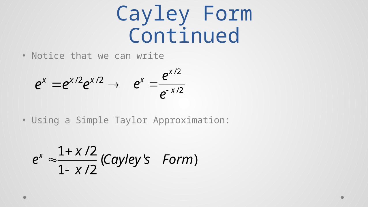
• Notice that we can write

• Using a Simple Taylor Approximation:

2/2/ xxx eee 2/

2/

x

xx

e

ee

)'(2/1

2/1FormsCayley

x

xex

Cayley FormContinued

• Writing the previous result in terms of the propagator

or

• This is like taking a half step forward from and a half step back from

• We replace E with the Hamiltonian operator to get a new set of tridiagonal matriceso Notice that left and right hand sides are complex conjugates of each other, only need to find one

matrix explicitly

2/1

2/11

tiE

tiEnn

nn tiEtiE 2/12/1 1

1 nn

Cayley Form Continued

• We have

• Let and

nj

nJj

nj

nj

nJ

nj xm

tiVti

xm

ti

xm

ti

xm

titi

xm

ti

xm

ti12212

112

12

112 422

14422

14

24 xm

ti

2ti

nj

nJj

nj

nj

nJj

nj VV 11

11

111 2121

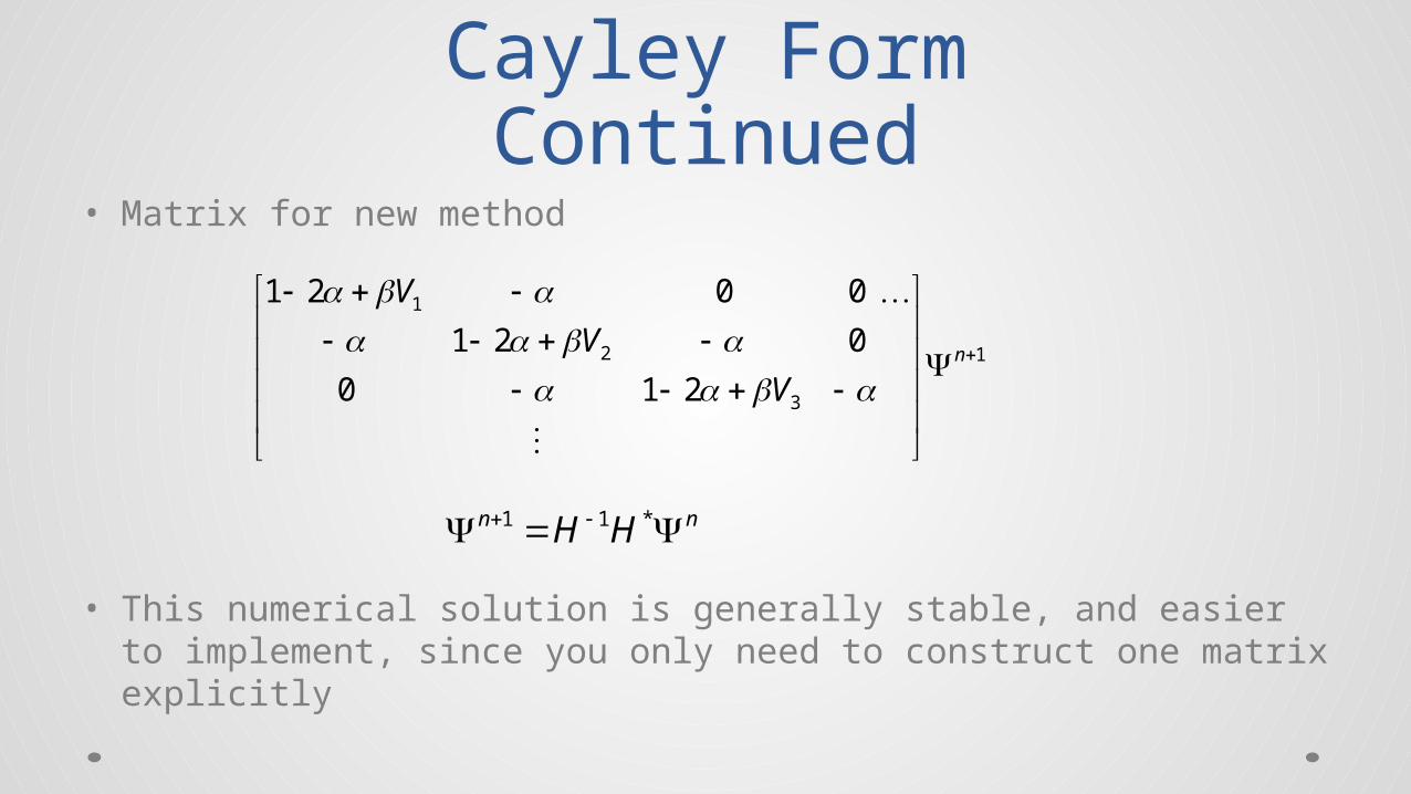
Cayley FormContinued

• Matrix for new method

• This numerical solution is generally stable, and easier to implement, since you only need to construct one matrix explicitly

1

3

2

1

210

021

0021

n

V

V

V

nn HH *11

Simulating Electron Motion• Now we have a numerical solution for the Schrodinger Equation

• We need to review units suitable for quantum mechanics

• We need to choose a form for our initial wavefunctiono Something with a known analytic solution so we can compare to numerical solution

Quantum Scale• SI units are far too large to study quantum effects• We write everything in terms of electron volts, angstroms, and

femtoseconds

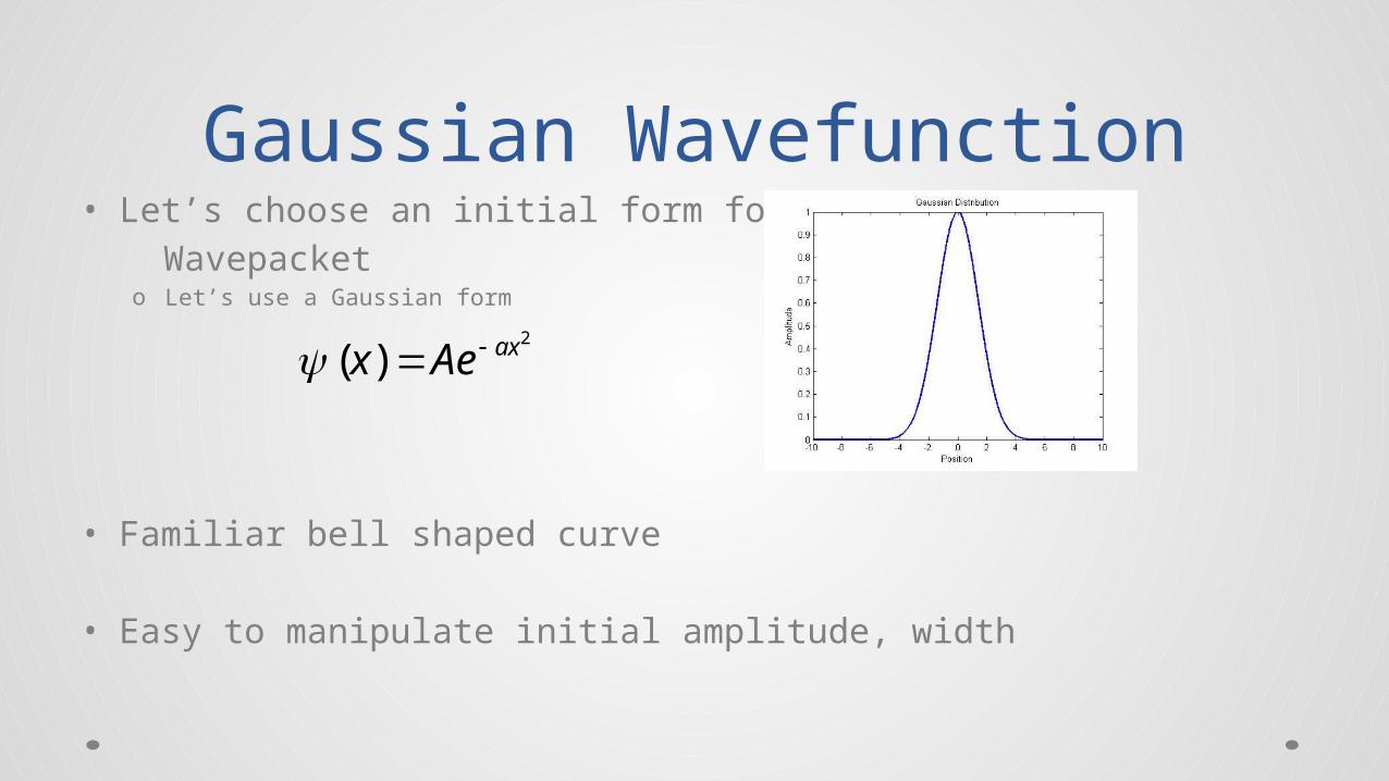
Gaussian Wavefunction• Let’s choose an initial form for the Wavepacket

o Let’s use a Gaussian form

• Familiar bell shaped curve

• Easy to manipulate initial amplitude, width

2

)( axAex

Analytic SolutionGaussian Wavefunction

xikax eAex 02

)(

1*4/1

2

a

A

dxexk ikx )(2

1)(

akkeak 4/)(4/1 20)2()(

•Start with

•Normalize

•Fourier transform to momentum space

Analytic SolutionContinued

dkeektx iEtikx /)(2

1),(

m

kE

2

22

m

tkmxik

ea

tx 2

)2(max24/1

2

002

2),(

mati /21

•Fourier transform back to position space adding time dependence

•Note that energy depends on momentum

•And after hours of Fourier transforms and simple algebra mistakes…

Comparison of Numerical and Analytic Solutions

Potential Barriers• Quantum level: don’t talk about forces, talk about potential energy

• Part of wavepacket usually reflected, and part always transmitted through a barrier (tunneling)

• Can measure how much transmitted and reflected

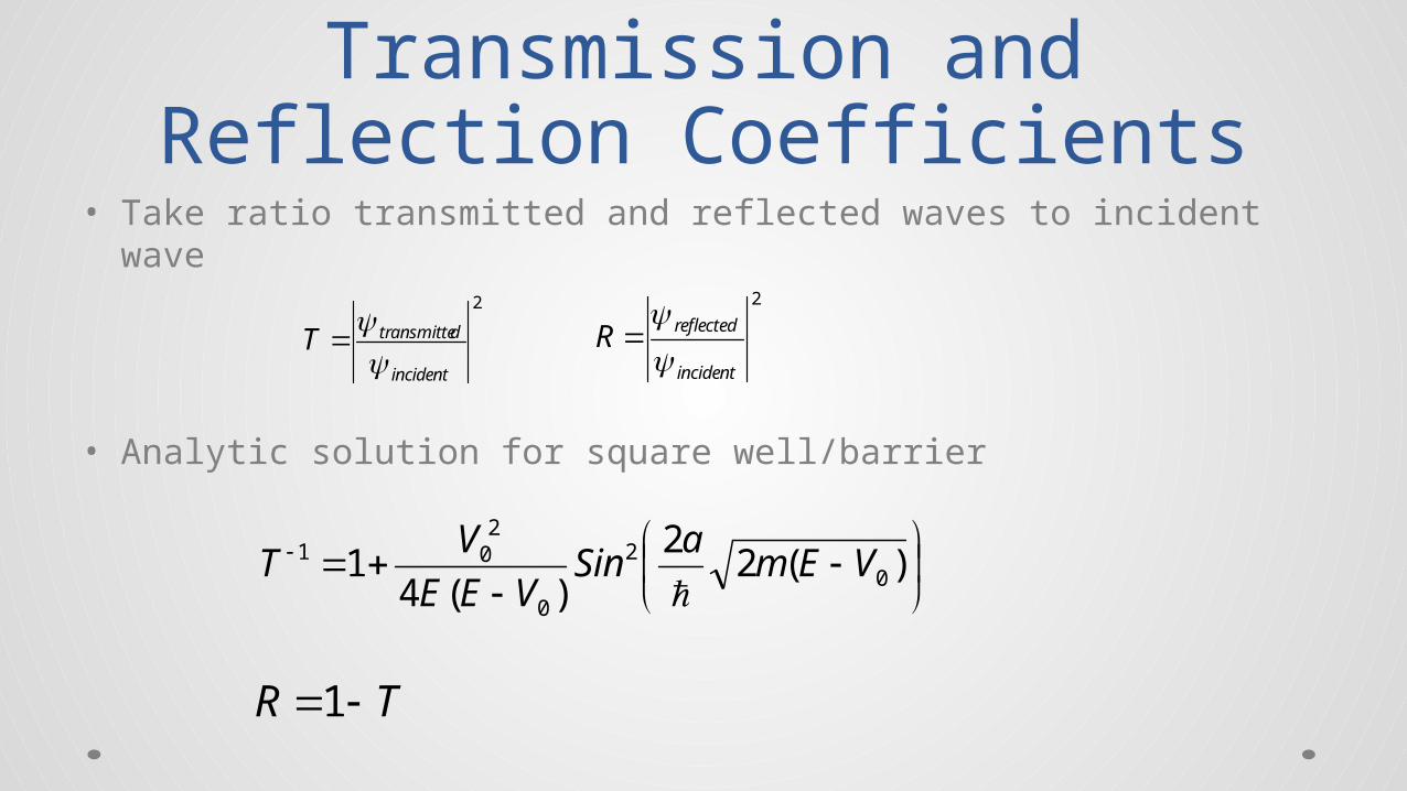
Transmission and Reflection Coefficients

• Take ratio transmitted and reflected waves to incident wave

• Analytic solution for square well/barrier

2

incident

dtransmitteT

2

incident

reflectedR

TR 1

)(2

2

)(41 0

2

0

201 VEm

aSin

VEE

VT

Simple PotentialBarrier

Reflection CoefficientsAnalytic: 0.3210Numerical: 0.3051

Transmission CoefficientsAnalytic: 0.6790Numerical: 0.6949

Simple PotentialWell

Reflection CoefficientsAnalytic: 0.0531Numerical: 0.0447

Transmission CoefficientsAnalytic: 0.9469Numerical: 0.9553

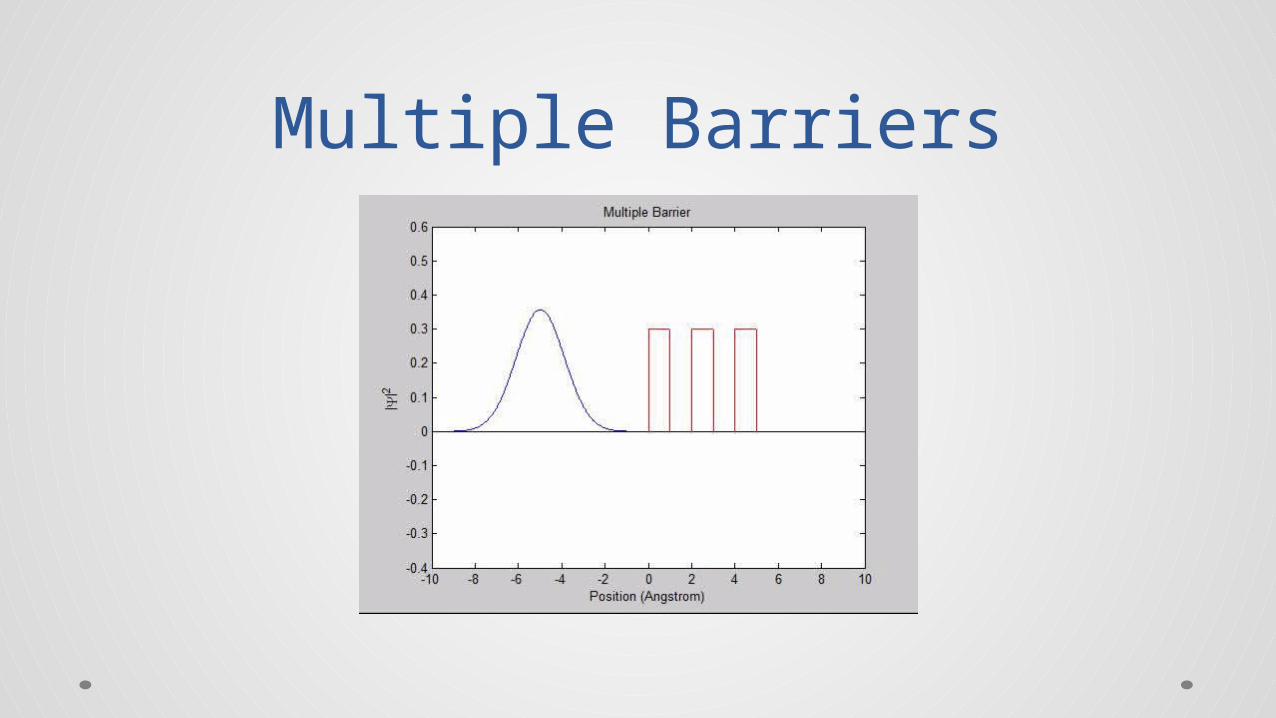
Multiple Barriers

Energy Space• is a function of space and time

• We can transform it to a function of space and energy through a Fourier transform

• Lets you see how energy distributed over space

),( tx

dtetxEx iEt /),(2

1),(

Energy Space• In this simulation, we perform a Fourier transform each time after

we propagate the electron through a barriero Note how the plane wave components change after interacting with the barrier

Infinite Square WellReview

• Particle bounded by infinitely high potential barriers

• Particle will bounce back and forth forever

• Probability outside walls is zero 0

Implicit Boundary Conditions• The simulated space is necessarily finite

• Algorithm simulates behavior for any realistic values of position

• Wavefunction undefined outside finite space

• Inadvertently create infinite square well

Boundary Behavior

Absorbing Potential• Can artificially decrease probability particle exists

• Construct an imaginary (or complex) potential

• Probability density decreases as particle moves through potential

• Can’t completely destroy particle

Free Space Propagation withAbsorbing Potential

• Potential is of form 2ixV

Summary• Numerical methods can be used to accurately model physics –

classical and non-classical

• The Crank-Nicolson method is an accurate method of modeling quantum behavioro Through free space, potential barriers, in other bases (momentum, energy, etc.)

• Numerical computation can have unexpected resultso Such as implicit boundary conditions

Future Research• Continue with 1D

o Increases accuracy of propagation through barriers—transmission and reflection coefficientso Use energy space transformation to build library of plane wave signatures for various potentials

• Move to 2D/3Do More complicatedo Can’t use Crank-Nicolson anymore

• Too computationally demanding• Matrix of ~1000 elements to matrix of ~1000x1000x1000 elements for 3D!

o Study Taylor series approximations