Simulation and Performance Evaluation of Finned-Tube CO

HAL Id: hal-00595946https://hal.archives-ouvertes.fr/hal-00595946

Submitted on 26 May 2011

HAL is a multi-disciplinary open accessarchive for the deposit and dissemination of sci-entific research documents, whether they are pub-lished or not. The documents may come fromteaching and research institutions in France orabroad, or from public or private research centers.

L’archive ouverte pluridisciplinaire HAL, estdestinée au dépôt et à la diffusion de documentsscientifiques de niveau recherche, publiés ou non,émanant des établissements d’enseignement et derecherche français ou étrangers, des laboratoirespublics ou privés.

Simulation and Performance Evaluation of Finned-TubeCO Gas Coolers for Refrigeration Systems

Y.T. Ge, R.T Cropper

To cite this version:Y.T. Ge, R.T Cropper. Simulation and Performance Evaluation of Finned-Tube CO Gas Cool-ers for Refrigeration Systems. Applied Thermal Engineering, Elsevier, 2009, 29 (5-6), pp.957.�10.1016/j.applthermaleng.2008.05.013�. �hal-00595946�

https://hal.archives-ouvertes.fr/hal-00595946

https://hal.archives-ouvertes.fr

Accepted Manuscript

Simulation and Performance Evaluation of Finned-Tube CO2 Gas Coolers for

Refrigeration Systems

Y.T. Ge, R.T Cropper

PII: S1359-4311(08)00221-4

DOI: 10.1016/j.applthermaleng.2008.05.013

Reference: ATE 2507

To appear in: Applied Thermal Engineering

Received Date: 18 January 2008

Revised Date: 1 May 2008

Accepted Date: 11 May 2008

Please cite this article as: Y.T. Ge, R.T Cropper, Simulation and Performance Evaluation of Finned-Tube CO2 Gas

Coolers for Refrigeration Systems, Applied Thermal Engineering (2008), doi: 10.1016/j.applthermaleng.

2008.05.013

This is a PDF file of an unedited manuscript that has been accepted for publication. As a service to our customers

we are providing this early version of the manuscript. The manuscript will undergo copyediting, typesetting, and

review of the resulting proof before it is published in its final form. Please note that during the production process

errors may be discovered which could affect the content, and all legal disclaimers that apply to the journal pertain.

http://dx.doi.org/10.1016/j.applthermaleng.2008.05.013



ACCEPTED MANUSCRIPT

1

Simulation and Performance Evaluation of Finned-Tube CO2

Gas Coolers for Refrigeration Systems

Y.T. Ge a,*, R. T Cropper b

a Mechanical Engineering, School of Engineering and Design ,Brunel University

,Uxbridge, Middlesex , UB8 3PH, UK

b Formerly School of Engineering, North East Wales Institute, Plas Coch Campus, Mold

Road, Wrexham, L11 2AW, UK

_____________________________________________________________________

Abstract

This paper describes a detailed mathematical model and its application for air-cooled

finned-tube CO2 gas coolers. The model has been developed utilizing a distributed

method which is necessary to predict accurately the great variation of both refrigerant

thermophysical properties and local heat transfer coefficients during CO2 gas cooling

processes. The modelling method also enables performance analyses with different

circuit arrangements and changed structure parameters in gas coolers to be assessed.

The model has been validated with the test results from a published literature by

ACCEPTED MANUSCRIPT

2

comparing the gas temperature profiles along the coil pipes from refrigerant inlet to

outlet at different operating states. With the aim of increasing the heat capacity or

minimizing the approach temperature for a gas cooler, the validated model is used to

carry out performance simulation and analysis when the circuit arrangement of the

original heat exchanger is redesigned. It is found that the approach temperature and the

heat capacity are both improved with the increase of heat exchanger circuit numbers.

Key Words: model, CO2, gas cooler, simulation and validation, performance analysis.

_____________________________________________________________________

Nomenclature

A area (m2) Subscripts

Cp specific heat at constant pressure (J kg-1K-1) a air

C capacity rate (W K-1) f friction

d diameter(m) h hot side

D depth (m) i inner, ith grid

f friction factor j jth grid

G mass flux (kg m-2 s-1) k kth grid

h enthalpy(J kg-1) min minimum

H height (m) max maximum

i, j, k coordinates o outer

m mass flow rate (kg s-1) r refrigerant

ACCEPTED MANUSCRIPT

3

P pressure (Pa) wi inner pipe wall

q heat transfer per square meter (W m-2)

Q heat transfer (W)

R resistance (K W-1)

s perimeter of inner pipe (m)

T temperature (K)

u velocity (m s-1)

U overall heat transfer coefficient (W m-2 K-1)

Va air velocity (m s-1)

W width (m)

z length (m)

Greek symbol

heat transfer coefficient (W m-2 K-1)

efficiency

difference

density (kg m-3)

shear stress (N m-2)

effectiveness

1. Introduction

Carbon dioxide (CO2), as a natural

refrigerant, has been attracting more and

more attention in the applications

involving refrigeration, heat pump and

ACCEPTED MANUSCRIPT

4

air conditioning systems. Compared

with the conventional refrigerants like

R22, R134a and R404A etc., CO2 is

more environmentally friendly with

zero Ozone-Depleting Potential and

very low direct Global Warming

Potential. The CO2 refrigerant has also

favourable thermophysical properties

like higher values of density, latent heat,

specific heat, thermal conductivity and

volumetric cooling capacity, and lower

value of viscosity. However, CO2

refrigerant has a quite high operating

pressure because of its low critical

temperature (31.1 °C) and high critical

pressure (73.8 bar). In a CO2

refrigeration system when heat is

rejected to ambient air at temperatures

close to or above 31.1 °C, the critical

temperature of CO2, the refrigeration

cycle is said to operate in a transcritical

mode. The conventional air cooled

condenser is therefore replaced with a

gas cooler. As a main component of a

CO2 transcritical refrigeration system,

the gas cooler’s performance greatly

affects a system’s efficiency and is thus

worthy of further investigation.

In its simplest form a transcritical

CO2 cycle is thermodynamically less

efficient compared with a conventional

vapour-compression cycle [1]. Bullock

[2] compared the performance of a CO2

transcritical cycle with a R22 system for

an air conditioning application. He

found that CO2 systems were less

efficient than R22 systems by 30% in

the cooling mode. Similar conclusions

were obtained by Robinson and Groll

[3] and Aarlien and Frivik [4]. The

operating efficiency for the CO2 system

can however be improved through the

use of an expansion turbine, a liquid-

line/suction-line heat exchanger (llsl-

hx), and significant performance

improvements in system equipment

such as compressor, evaporator or gas

cooler. In CO2 refrigeration system

ACCEPTED MANUSCRIPT

5

with a transcritical cycle, at fixed

refrigerant gas cooler outlet temperature

and evaporating temperature, there is an

optimum high-side pressure such that

the cooling COP in the system can

reach a maximum [5-7]. The refrigerant

high-side pressure can be controlled by

adjusting the back (high-side) pressure

of the installed expansion valve in the

system [1]. It is known that at a constant

evaporating temperature the maximum

cooling COP is increased greatly with

lower refrigerant temperature at the gas

cooler exit. The temperature difference

between the refrigerant outlet and

incoming ambient air is called approach

temperature (AT) for an air-cooled gas

cooler. The minimization of the

approach temperature will greatly affect

the system efficiency [8] this being

mainly dependent on the optimal design

of the heat exchanger. Consideration of

circuit arrangements and structural

parameters will affect the optimal

design for the heat exchanger, an

efficient and economic way to effect

this analysis is to utilize the simulation

technique.

In CO2 transcritical cycles, finned-

tube gas coolers are not as popular as

aluminium minichannel heat exchangers

which have advantages of less risk of

high pressure stresses, light weight and

compactness and are widely used in

automobile air conditioning. Therefore,

a great deal of research and

development effort has been put into

minichannel heat exchangers [9-11].

However, because of the lower cost, the

finned-tube coils are still believed as

competent types of gas coolers.

Theoretically three modelling methods

could be used in the performance

analysis of such gas coolers, -NTU or

LMTD i.e. lumped method, tube-in-

tube, and distributed method. Since

there is rapid change of the CO2

thermophysical properties with

ACCEPTED MANUSCRIPT

6

temperature during an isobaric gas

cooling process, it is not practical to use

the -NTU or LMTD method to

simulate gas coolers [12]. The tube-in-

tube method developed from the

research of Domanski [13,14] was

utilized in the simulation of a gas cooler

by Chang and Kim [15]. By means of

the model simulation, the effects of

some coil structural parameters on the

performance of the gas cooler were

investigated. It was found from the

simulation results that the approach

temperature can be decreased with

increased heat exchanger front area.

Although a significant modelling

improvement can be realized by this

method, a more detailed modelling

strategy, distribution method, is still

expected to further enhance the

simulation accuracy and therefore

obtain more reliable conclusions. Due to

higher simulation accuracy, the

distributed method has been widely

used in modelling the finned-tube air

cooling evaporators and air cooled

condensers. A distributed computational

model for the detailed design of finned

coils (condensers or evaporators) has

been developed by Bensafi et al [16].

The model can simulate the finned coils

with non-conventional circuits, non-

uniform air distribution and different

structures of pipes and fins. However,

the correlations used in the calculations

of heat transfer coefficients and

pressure drops for both refrigerant and

air need be updated. In addition, the

types of refrigerants applied to the

model need be enhanced. Similarly, the

air-cooled condensers were modelled

with the distributed method by Casson

et al [17]. The model can be used in

optimal design of the internal circuits of

the heat exchangers and performance

comparison with R22 and its HFC

substitutes. This model was used by

Zilio et al [18] to validate the

ACCEPTED MANUSCRIPT

7

experimental research for CO2 gas

coolers and a systematic deviation was

realised. The suitable correlations to

predict CO2 heat transfer coefficients

were therefore tested. Recently, a

simulation and design tool to carry out

optimal design and performance

analysis for the air to refrigerant heat

exchangers, called CoilDesigner, was

introduced by Jiang et al [19]. Apart

from the powerful design and

simulation functions due to utilise the

distributed method, the design tool has

an advanced user friendly interface to

deal with the pre and post simulation

processes. However, the iteration

methods for both refrigerant and air

sides haven’t presented in the paper.

The distributed method was used in a

gas cooler model by Sarkar et al [20]

but the heat exchanger was the type of

water cooled double pipe. To the

authors’ knowledge, in the public

literatures, it is hardly found that a gas

cooler model has been developed using

the distributed method. Although the

fundamental conservation equations

used in each coil element can be the

same when using the distributed method

to set up the models, the simulation

results could be largely different. The

main reasons are the different

assumptions when using the

conservation equations, the various

correlations of heat transfer coefficients

and pressure drops for both refrigerant

and air sides, and also the diverse

solving and iteration methods used in

the models.

This paper describes the

mathematical modelling of a finned-

tube air-cooled CO2 gas cooler by

means of distributed method. The

update correlations of heat transfer

coefficients and pressure drops for both

refrigerant and air sides are utilised. An

efficient solving method is proposed in

the simulation. The model is validated

ACCEPTED MANUSCRIPT

8

with the test results from published

literature. The validated model is then

utilized to explore the potential for

improved designs of gas coolers to

achieve the minimum approach

temperature and maximum system

operating efficiency.

2. Model descriptions

The distributed method is used in

developing the simulation model of

finned-tube air-cooled CO2 gas coolers.

A diagram with sub elements of the coil

in three-dimensional (3-D) space for the

model is schematically drawn in Figure

1. Tubes are arranged parallel to i

direction, j is specified in the

longitudinal direction, while k is in the

transverse direction. Air is flowing

parallel to j direction and refrigerant is

assumed in approximate counter-cross

direction to air for this sample. The

selection of the number of small

elements in i direction is arbitrary from

one to infinity. The larger this value is,

the more accurate the simulation will

be, but expensive computing time will

be sacrificed. The coordinate of each

divided element in the 3-D space can

then be determined. The coordinate

value i represents the number of sub-

elements for each pipe, selected by the

model, j corresponds to pipe numbers in

longitudinal paths starting from the air

inlet, while k equals the tube numbers in

the transverse path originating from the

bottom. Therefore, the state point of

either refrigerant or air at each specified

sub-element in the 3-D space can be

positioned with its corresponding

coordinate values i, j and k, which vary

according to the circuit number and pipe

number. The pipe number starts from

refrigerant inlet to refrigerant outlet for

each circuit. The solving routine firstly

starts from the circuit loop if there is

more than one circuit for the coil. For

ACCEPTED MANUSCRIPT

9

each circuit, the simulation will run

through each numbered pipe starting

from refrigerant inlet and then the

element loop for each pipe. The whole

modelling work depends on setting up

the conservation equations for each sub-

element and an efficient routine to solve

these equations. The solutions for one

sub-element can be used as the inputs

for the next sub division. The air side

parameters for each element which are

normally unknown initially will be

firstly assumed. These parameters will

be updated by next time iteration. The

total heating load of the gas cooler is

calculated at the end of each iteration.

The iteration will carry on until all the

loops are cycled and the total heating

loads for two continuous iterations are

nearly not changed.

2.1 Refrigerant side conservation

equations

Before setting up the refrigerant side

conservation equations for each

element, the following assumptions are

proposed:

System is in steady state.

No heat conduction in the

direction of pipe axis and nearby

fins.

Air is in homogeneous

distribution, that is, air-facing

velocity to each element is the

same.

No contact heat resistance

between fin and pipe.

Refrigerant at any point in the

flowing direction is in thermal

equilibrium condition.

Mass equation:

0)( rmdzd

(1)

Momentum equation:

wi

wiwir

i A

s

dz

dPum

dz

d

A

)(

1 (2)

Energy equation:

ACCEPTED MANUSCRIPT

10

qdhmdzd

or )()( (3)

The above equations can be easily

discretized as below for a sub-element

shown in Figure 1 with coordinate from

(i, j, k) to (i+1, j, k). The dimensions of

the sub-element at (i, j, k) directing to i,

j, k are zi , zj and zk respectively.

Mass equation:

0),,(),,1( kjirkjir mm (4)

Momentum equation:

fkjirkjiri

PPumumA

])()[(1

),,(),,1(

(5)

where, i

if d

zGfP

2

2 (6)

Energy equation:

io

kjirkjir

zqd

hmhm

)(

)()( ),,(),,1(

(7)

The conservation equations can also be

applied for the airside calculation. The

pressure drop calculation is used instead

of the momentum equation and heat

transfer calculation is included in the

energy equation for this side. In

addition, there is a heat balance between

the air and refrigerant sides for each

element.

Fig. 1. Three-dimensional coordinate of sub elements in the coil for the gas cooler

model

2.2 Airside Heat Transfer

ACCEPTED MANUSCRIPT

11

NTU- method is used in the

calculation of heat transfer for airside in

one grid section.

)],,(),,([min kjiTkjiTCQ ara (8)

where the effectiveness is calculated

as below:

)exp(1

Cfor )exp(1

max

maxmin

max

C

UAwhere

CC

Ch

(9)

and,

)exp(1

))exp(1(

min

max

min

min

max

C

UA where

CC forC

C

C

Chmin

(10)

The product UA (overall heat-transfer

coefficient times area) can be calculated

as:

1

00

)11

( rr

ia A

RA

UA

(11)

where Ri is the sum of heat conduction

resistances through the pipe wall and

fin.

The heat transfer from airside can be

calculated as:

)],,(),,([),,(

)],,(

),1,([),,(),,(

kjiTkjiTkjiUA

kjiT

kjiTkjiCpkjimQ

ar

a

aaaa

(12)

The parameters at grid points (i+1, j,

k) for refrigerant and (i, j+1 ,k) for air

can be obtained when equations (4) to

(12) are solved together.

The accurate model prediction also

relies on the precise calculations of fluid

properties, heat transfer coefficients and

pressure drops in both refrigerant and

air sides. The CO2 refrigerant properties

are calculated using subroutines from

the National Institute of Standards and

Technology software package

REFPROP [21]. For calculating the

refrigerant heat transfer coefficient, the

ACCEPTED MANUSCRIPT

12

correlation from Pitla et al. is utilized

[22]. The friction pressure drop is

calculated in equation (6) and the

Blasius equation [23] is used to

calculate the friction factor f. The air

side heat transfer and friction

coefficients are computed using the

correlations by Wang et al [24] [25].

3. Model validations

To develop a performance database

for the component design in CO2

transcritical cycle, a special designed

test facility was set up by Hwang et al.

[26]. The test system was composed of

an air duct and two environmental

chambers that house an evaporator, a

gas cooler, an expansion valve and a

compressor. By means of this test rig, a

set of parametric measurements at

various inlet air temperatures and

velocities, refrigerant inlet

temperatures, mass flow rates and

operating pressures were carried out on

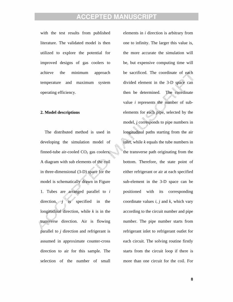
a specified CO2 gas cooler. The side

view of the circuit arrangement for the

tested gas cooler is shown in Figure 2.

The air flow is from right to left and

refrigerant inlet is at the upper left

numbered with “0” and the refrigerant

outlet is at the lower right numbered

with “54”for the heat exchanger. The

dash lines in the Figure indicate the U-

bends of the rear side noted with odd

numbers, while the solid lines signify

the U-bends of the front side noted with

even numbers. To measure the variation

of refrigerant temperature along the heat

exchanger pipes, numbers of

thermocouples were attached on the

outside surfaces of the front side U-

bend pipes and at refrigerant inlet and

outlet as well. These thermocouples

were well insulated to get more accurate

measurement. The structural

specification of the gas cooler is listed

in Table 1.

ACCEPTED MANUSCRIPT

13

Fig. 2. Tested gas cooler (Coil A) with numbered pipes

The test conditions, 36 in total, are

listed in Table 2. Each test condition

contains the measurements of air inlet

temperature, air velocity, refrigerant

inlet temperature, refrigerant inlet

pressure and refrigerant mass flow rate.

These measurements and the coil

structural parameters will be used as

model inputs and parameters

respectively. The predicted refrigerant

temperature profile at each test

condition is therefore compared with

the corresponding test result in order to

validate the model. To save space,

comparison results for twelve test

conditions with numbers 1 to 3, 10 to

12, 19 to 21 and 25 to 27, listed in Table

2 are selected and shown in Figure 3 to

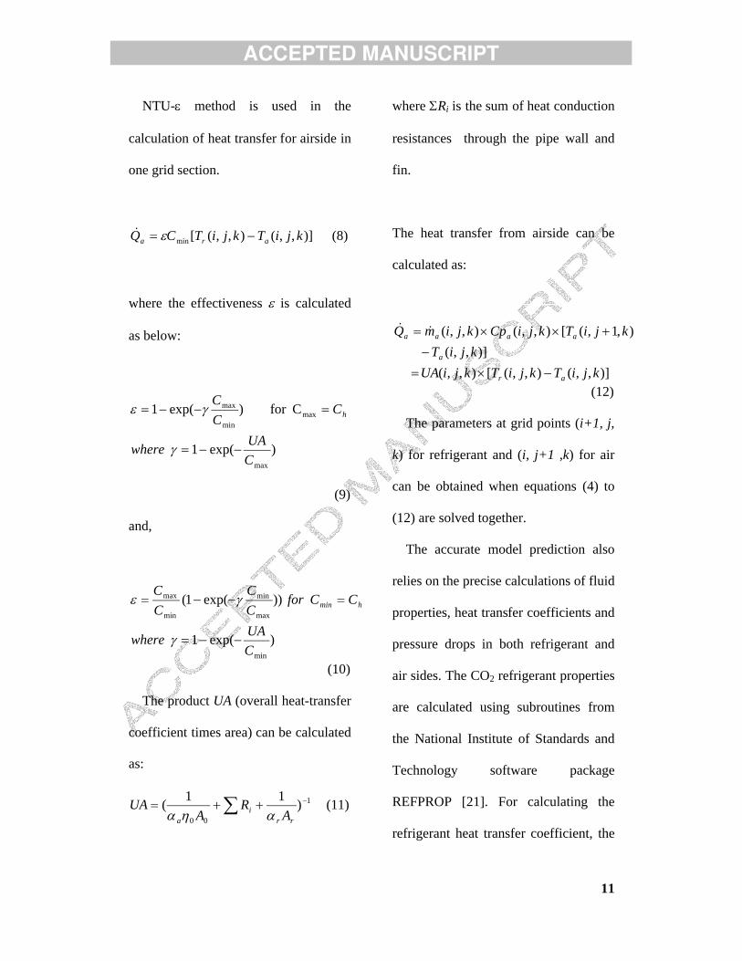
6 respectively. It is seen from both

simulation and test results that a sharp

refrigerant temperature decrease occurs

in the third pipe row (j=3), pipes

numbered from 0 to 18 in Figure 2. The

temperature changing rates in the

second (j=2) and first rows (j=1) are

gradually reduced. In addition, at

constant refrigerant pressure and mass

flow rate, similar refrigerant inlet

temperature and unchanged air inlet

temperature, refrigerant temperature at

any specified location is always lower

for higher front air velocity. This is

because that the heat transfer is

enhanced with higher front air velocity.

The predicted refrigerant temperature

profile for each test condition matches

ACCEPTED MANUSCRIPT

14

fairly well with that of test result. For

all the test conditions, the refrigerant

temperatures at the gas cooler outlet are

predicted and compared with those of

test results, as shown in Figure 7. The

temperature discrepancies between

simulation and the test results for

refrigerant outlet temperatures are

mostly within ±2 °C when air front

velocity is above 1m/s. The bigger

errors are predominantly caused when

the air front velocity is at 1m/s. The

correlation of airside heat transfer

coefficient at lower air velocity needs

therefore be further revised. It is

concluded that the simulation can fairly

represent the test results and the model

is therefore validated.

Table 1 Specification of the tested gas cooler

Table 2 Test conditions

Fig. 3. Comparison of simulation with test results of test condition Nos. 1 to 3 for

refrigerant temperature profile.



ACCEPTED MANUSCRIPT

15





Fig. 7. Comparison of simulation with test results of all test conditions for refrigerant

temperatures at gas cooler outlet.

4. Model applications

The validated model is used to

explore the possibility of minimising

the approach temperature by means of

redesigning the circuits of the gas

cooler. As shown in Figure 2, the

original gas cooler, named Coil A, has

just one circuit for the total 54 pipes.

The coil is now rearranged into two

circuits named Coil B and three circuits

called Coil C, as shown in Figure 8. In

each pipe circuit, there are 27 pipes for

Coil B and 18 pipes for Coil C. All

other structural parameters in both Coil

B and Coil C are kept the same as those

in Coil A. Under the same test

conditions listed in Table 2, the

simulation is run and the approach

temperatures and heating loads are

predicted and compared for Coil A, Coil

ACCEPTED MANUSCRIPT

16

B and Coil C, as shown in Figures 9 , 10 ,11 and 12 respectively.

Fig. 8. Two new circuit arrangements for the tested gas cooler

It is seen from the simulation results

that at any test condition, the approach

temperature for coil C is slightly less

than that of Coil B but much smaller

than that of coil A, especially when total

refrigerant mass flow rate is lower. The

maximum approach temperature

decrease by modifying coil A to coil C

can reach to 12.1 k at test condition 25.

In the mean time, the approach

temperature is decreased with increased

air front velocity when other parameters

are unchanged. In addition, the

approach temperature is generally

increased with higher ambient air

temperature except for some points such

as test 1 and test 10 because of the

effects of different inlet gas

temperatures. The lowest approach

temperature predicted in Coil C can

bring the highest heating load among

these coils at any test condition, as

shown in Figures 11 and 12. The

maximum heating load increase rate by

using coil C to replace coil A can be

52% at test condition 5. Consequently

at any test condition Coil A has the

lowest heating load compared with the

other two coils. At any test condition,

Coil C will therefore have the lowest

gas outlet enthalpy which will produce

highest cooling effect and consequently

highest system cooling COP.

ACCEPTED MANUSCRIPT

17

Fig. 9. Simulated approach temperatures for Coil A, B and C at various test conditions

(1-18).


(19-36).

Fig. 11. Simulated heating loads for Coil A, B and C at various test conditions

(1-18).


(19-36).

5. Conclusions

A steady state model for finned-tube

air-cooled gas coolers has been

developed by means of distributed

simulation method. Such simulation

method is necessary to accurately model

a gas cooler since a notable variation of

gas thermophysical parameters and

local heat transfer coefficients is

expected during the gas cooling process.

A proposed model solving strategy

when distributed method is used can

efficiently run the simulation. The gas

cooler model is validated with the

experimental results from published

ACCEPTED MANUSCRIPT

18

literature at different test conditions.

The validated model is utilized to

investigate the effect of varied pipe

circuit arrangements on the performance

of gas coolers and some conclusions are

obtained:

The gas temperature is

decreased with the highest rate

at the beginning along the pipe

from refrigerant inlet to outlet.

With increased pipe circuits, the

gas heat transfer coefficients

inside the pipes will be

increased and therefore at any

test condition, the approach

temperature will be decreased

and the heating load will be

increased. From the simulation

results, a maximum 12.1 k

approach temperature decrease

and 51.5% heating load increase

can be achieved when gas cooler

pipe circuit numbers are

increased .Therefore, in the gas

cooler optimal design, more

circuit numbers need be

considered.

The approach temperature is

decreased with an increased air

front velocity.

The lower approach temperature

can induce higher heating load

of the gas cooler and

consequently bring higher

cooling capacity and system

cooling COP.

An accurate gas cooler model

can help in the optimal design of

the gas cooler.

References

[1] E.A. Groll, J.H. Kim, Review of

recent advances toward

transcritical CO2 cycle technology,

HVAC&R Research, Vol 13, n3,

May 2007, 499-520.

ACCEPTED MANUSCRIPT

19

[2] C.E. Bullock, Theoretical

performance of carbon dioxide in

subcritical and transcritical cycles.

ASHRAE/NIST Refrigeration

Conference, Refrigerants for 21st

Century, 1997, 20-26.

[3] D.M. Robinson, E.A. Groll,

Efficiencies of transcritical CO2

cycles with and without an

expansion turbine, International

Journal of Refrigeration 21(7),

1998, 577-589.

[4] R. Aarlien, P.E. Frivik, Comparison

of practical performance between

CO2 and R-22 reversible heat

pumps for residential use.

Proceedings of Natural Working

Fluids, IIF-IIR Commision 2,

Oslo, Norway, 1998,388-398.

[5] S.M. Liao, T.S. Zhao, A. Jakobsen,

A correlation of optimal heat

rejection pressures in transcritical

carbon dioxide cycles, Applied

Thermal Engineering 20, 2000,

831-841.

[6] F. Kauf, Determination of the

optimum high pressure for

transcritical CO2-refrigeration

cycles, Int. J. Therm. Sci. 38,

1999, 325-330.

[7] Y. Chen, J. Gu, The optimum high

pressure for CO2 transcritical

refrigeration systems with internal

heat exchangers, International

Journal of Refrigeration

28,2005,1238-1249.

[8] X. Fang, C. Bullard, P. Hrnjak.

Heat transfer and pressure drop of

gas coolers, ASHRAE Trans

,107(1), 2001, 255-266.

[9] J.M. Yin, C.W. Bullard, P.S.

Hrnjak, R-744 gas cooler model

development and validation,

International Journal of

Refrigeration, 24, 2001, 692-701.

[10] T.M. Ortiz, D. Li, E.A. Groll,

Evaluation of the performance

ACCEPTED MANUSCRIPT

20

potential of CO2 as a refrigerant in

air-to-air air conditioners and heat

pumps:system modeling and

analysis, Final report, ARTI-

21CR/610-10030, December 2003.

[11] J. Pettersen, A. Hafner, G.

Skaugen, H. Rekstad.

Development of compact heat

exchangers for CO2 air-

conditioning systems, International

Journal of Refrigeration, 21(3),

1998, 180-193.

[12] M.H. Kim, J. Pettersen, C.W.

Bullard. Fundamental process and

system design issues in CO2

vapour compression systems.

Progress in Energy and

Combustion Science, 30, 2004,

119-174.

[13] P.A. Domanski, EVSIM-An

evaporator simulation model

accounting for refrigerant and one-

dimensional air, NISTIR-89-4133.

Washington, DC:NIST,1989.

[14] P.A. Domanski, D. Yashar,

Optimization of finned-tube

condensers using an intelligent

system, International Journal of

Refrigeration 30(2007) 482-488.

[15] Y.S. Chang, M.S. Kim. Modelling

and performance simulation of a

gas cooler for CO2 heat pump

system. V13,n3, HVAC&R

Research, May 2007, 445-456.

[16] A. Bensafi, S. Borg and D. Parent,

CYRANO: a computational model

for the detailed design of plate-fin-

and-tube heat exchangers using

pure and mixed refrigerants, Int. J.

Refrigeration. Vol. 20 (1997),

No.3, 218-228.

[17] V. Casson, A. Cavallini, L.

Cecchinato, D.Del Col, L. Doretti,

E. Fornasieri, L. Rossetto, C. Zilio,

Performance of finned coil

condensers optimized for new

HFC refrigerants, ASHRAE

ACCEPTED MANUSCRIPT

21

Transactions, (2002) 108 (2), 517-

527.

[18] C. Zilio, L.Cecchinato, M. Corradi,

G. Schiochet, An assessment of

heat transfer through fins in a fin-

and-tube gas cooler for

transcritical carbon dioxide cycles.

Vol. 30, 2007, No. 3, HVAC&R

Research.

[19] H. Jiang, V. Aute, R. Radermacher,

CoilDesigner: a general-purpose

simulation and design tool for air-

to-refrigerant heat exchangers,

International Journal of

Refrigeration 29, 2006, 601-610.

[20] J. Sarkar, S. Bhattacharyya, m. R.

Gopal. Simulation of a transcritical

CO2 heat pump cycle for

simultaneous cooling and heating

applications. International Journal

of Refrigeration 29, 2006, 735-

743.

[21] M. McLinden, S.A. Klein, E.W.

Lemmon, A.P. Peskin. NIST

thermodynamic and transport

properties of refrigerants and

refrigerant mixtures- REFPROP,

v6.0, NIST Standard Reference

database 23,1998.

[22] S.S. Pitla, E.A. Groll,S.

Ramadhyani. New correlation to

predict the heat transfer coefficient

during in-tube cooling of turbulent

supercritical CO2. International

Journal of Refrigeration 25, 2002,

887-895

[23] F.P. Incropera, D.P. DeWitt.

Introduction to heat transfer. 3rd ed.

New York:John Wiley

&Sons,1996.

[24] C.C. Wang, J.Y. Jang, N.F. Chiou,

1999a, A heat transfer and friction

correlation for wavy fin-and-tube

heat exchangers, Int. J. of Heat

Mass Transfer 42, 1919-1924.

[25] C.C. Wang, W.S. Lee, W.J. Sheu,

2001, A comparative study of

compact enhanced fin-and-tube

ACCEPTED MANUSCRIPT

22

heat exchangers, Int. J. of Heat

Mass Transfer 44, 3565-3573.

[26] Y.Hwang, D.H Jin, R. adermacher,

J.W. Hutchins. Performance

measurement of CO2 heat

exchangers, ASHRAE Trans.

2005, 306-316.

ACCEPTED MANUSCRIPT

Fig. 1. Three-dimensional coordinate of sub elements in the coil for the gas cooler model

Refrigerant in

Refrigerant out

Air

k

i

j

kz

j= j … 3 2 1k

k

4

3

2

1

jz

i= 1 2 3 4 … i

iz

cross-section perpendicular to i view from j direction

ACCEPTED MANUSCRIPT

Fig. 2. Tested gas cooler (Coil A) with numbered pipes

Refrigerant in

Airflow

Refrigerant out

0

10

11

12

13

14

15

16

17

1

2

3

4

5

6

7

8

946

47

48

49

50

51

52

53

37

38

39

40

41

42

43

44

45

18

26

25

24

23

22

21

20

19

35

34

33

32

31

30

29

28

27

36

54

ACCEPTED MANUSCRIPT

20

40

60

80

100

120

140

0 2 4 6 8 10 12 14 16 18 20 22 24 26 28 30 32 34 36 38 40 42 44 46 48 50 52 54

Pipe Number

Ref

rig

eran

t te

mp

erat

ure

(°C

)

Test: Va=1.0 m/sSimulation:Va=1.0 m/sTest:Va=2.0 m/sSimulation: Va=2.0 m/sTest :Va=3.0 m/s Simulation: Va=3.0 m/s

Operating States:Refigerant side: P=9 Mpa; Mass flow rate: 0.038 kg/sAir side: Inlet temperature=29.4 °C



ACCEPTED MANUSCRIPT

20

40

60

80

100

120

140

0 2 4 6 8 10 12 14 16 18 20 22 24 26 28 30 32 34 36 38 40 42 44 46 48 50 52 54

Pipe Number

Ref

rig

eran

t te

mp

erat

ure

(°C

) Test: Va=1.0 m/sSimulation:Va=1.0 m/sTest:Va=2.0 m/sSimulation: Va=2.0 m/sTest :Va=3.0 m/s Simulation: Va=3.0 m/s




ACCEPTED MANUSCRIPT

20

40

60

80

100

120

140

0 2 4 6 8 10 12 14 16 18 20 22 24 26 28 30 32 34 36 38 40 42 44 46 48 50 52 54

Pipe Number

Ref

rig

eran

t te

mp

erat

ure

(°C

) Test: Va=1.0 m/sSimulation:Va=1.0 m/sTest:Va=2.0 m/sSimulation: Va=2.0 m/sTest :Va=3.0 m/s Simulation: Va=3.0 m/s




ACCEPTED MANUSCRIPT

20

40

60

80

100

120

140

0 2 4 6 8 10 12 14 16 18 20 22 24 26 28 30 32 34 36 38 40 42 44 46 48 50 52 54

Pipe Number

Ref

rig

eran

t te

mp

erat

ure

(°C

)

Test: Va=1.0 m/sSimulation:Va=1.0 m/sTest:Va=2.0 m/sSimulation: Va=2.0 m/sTest :Va=3.0 m/s Simulation: Va=3.0 m/s




ACCEPTED MANUSCRIPT

25

30

35

40

45

50

55

25 30 35 40 45 50 55

Test (°C)

Sim

ula

tio

n (

°C)

Va=1.0 m/s

Va=2.0 m/s

Va=3.0 m/s

Test+2

Test-2 °C

Fig. 7. Comparison of simulation with test results of all test conditions for refrigerant

temperatures at gas cooler outlet.

ACCEPTED MANUSCRIPT

Fig. 8. Two new circuit arrangements for the tested gas cooler

Refrigerant in

Refrigerant out

0

1

2

3

4

5

6

7

8

18

19

20

21

22

23

24

25

16

15

14

13

12

11

10

9

17

260

1

2

3

4

5

6

7

8

18

19

20

21

22

23

24

25

16

15

14

13

12

11

10

9

17

26

Refrigerant in

Airflow

Refrigerant out

0

1

2

3

4

12

13

14

15

16

10

9

8

7

6

11

170

1

2

3

4

5

12

13

14

15

16

10

9

8

7

6

11

170

1

2

3

4

5

12

13

14

15

16

10

9

8

7

6

11

17

Coil B Coil C

ACCEPTED MANUSCRIPT

0

1

2

3

4

5

6

7

8

9

10

1 2 3 4 5 6 7 8 9 10 11 12 13 14 15 16 17 18

Test condition

Ap

pro

ach

tem

per

atu

re (

K)


(1-18).

Coil A Coil B Coil C

ACCEPTED MANUSCRIPT

0

2

4

6

8

10

12

14

16

18

20

19 20 21 22 23 24 25 26 27 28 29 30 31 32 33 34 35 36

Test condition

Ap

pro

ach

tem

per

atu

re (

K)

Fig. 10. Simulated approach temperatures for Coil A, B and C at various test

conditions (19-36).


ACCEPTED MANUSCRIPT

0

2

4

6

8

10

12

1 2 3 4 5 6 7 8 9 10 11 12 13 14 15 16 17 18

Test condition

Hea

tin

g l

oad

(kW

)


(1-18).


ACCEPTED MANUSCRIPT

0

2

4

6

8

10

12

14

16

18

20

19 20 21 22 23 24 25 26 27 28 29 30 31 32 33 34 35 36

Test condition

Hea

tin

g l

oad

(kW

)


(19-36).


ACCEPTED MANUSCRIPT

Table 1 Specification of the tested gas cooler

WHD [m] 0.610.460.05Dimension

Front area [m2] 0.281

Shape Raised lance

Fin pitch [mm] 1.5Fin

Thickness [mm] 0.13

No. of tubes row 3

No. of tubes per row 18

Tube outside diameter [mm] 7.9

Tube inside diameter [mm] 7.5

Tube

Tube shape smooth

ACCEPTED MANUSCRIPT

Table 2 Test conditions (including tested and simulated refrigerant outlet

temperatures)

Test

cond.

Air inlet

air temp.

[°C]

Air

velocity

[m/s]

Refri.

inlet

temp.

[C]

Refri. inlet

pressure

[MPa]

Refri.

flow rate

[kg/s]

Tested

Refri.

Outlet

temp. [°C]

Simu.

Refri. Outlet

temp. [°C]

1 29.4 1 118.1 9 0.038 40.4 38.0

2 29.4 2 109.5 9 0.038 33.5 33.5

3 29.4 3 113.5 9 0.038 31.3 31.5

4 29.4 1 124 10 0.038 41.5 36.9

5 29.4 2 118 10 0.038 32.3 31.2

6 29.4 3 117.1 10 0.038 31.1 30.3

7 29.4 1 128.8 11 0.038 40.4 34.3

8 29.4 2 123.5 11 0.038 31.7 30.4

9 29.4 3 123.1 11 0.038 30.9 29.9

10 35 1 121.3 9 0.038 43.1 40.6

11 35 2 119.4 9 0.038 39.8 38.8

12 35 3 118.8 9 0.038 38.2 37.9

13 35 1 127.7 10 0.038 45.5 41.9

14 35 2 122.6 10 0.038 38.7 37.9

15 35 3 122.2 10 0.038 37.2 36.6

16 35 1 133.3 11 0.038 46.0 40.9

17 35 2 128.9 11 0.038 38.0 36.6

18 35 3 128.4 11 0.038 36.7 35.6

ACCEPTED MANUSCRIPT

19 29.4 1 94.8 9 0.076 41.1 41.1

20 29.4 2 90.8 9 0.076 38.4 38.8

21 29.4 3 86.9 9 0.076 37.2 37.8

22 29.4 1 103.3 10 0.076 45.8 44.9

23 29.4 2 94.8 10 0.076 39.1 40.4

24 29.4 3 90.7 10 0.076 35.3 37.5

25 29.4 1 110.6 11 0.076 49.3 47.0

26 29.4 2 100.7 11 0.076 38.4 39.5

27 29.4 3 97.1 11 0.076 33.9 35.6

28 35 1 92.5 9 0.076 43.8 43.3

29 35 2 90 9 0.076 40.2 40.9

30 35 3 88.4 9 0.076 39.4 40.0

31 35 1 104.1 10 0.076 48.0 47.2

32 35 2 98.4 10 0.076 43.4 43.6

33 35 3 93.9 10 0.076 41.1 42.0

34 35 1 109.6 11 0.076 51.5 49.7

35 35 2 101.9 11 0.076 43.6 44.3

36 35 3 98.4 11 0.076 40.5 41.6

Documents

Simulation and Performance Evaluation of Finned-Tube CO