Embed Size (px)
Citation preview

7/29/2019 Simulation and Validation of Two-component Flow in a Void Recircu
http://slidepdf.com/reader/full/simulation-and-validation-of-two-component-flow-in-a-void-recircu 1/171
SIMULATION AND VALIDATION OF TWO-COMPONENT FLOW
IN A VOID RECIRCULATION SYSTEM
A Thesis
presented to
the Faculty of California Polytechnic State University,
San Luis Obispo
In Partial Fulfillment
of the Requirements for the Degree
Master of Science in Mechanical Engineering
by
Oscar Eduardo Daza
May 2011
7/29/2019 Simulation and Validation of Two-component Flow in a Void Recircu
http://slidepdf.com/reader/full/simulation-and-validation-of-two-component-flow-in-a-void-recircu 2/171
ii
© 2008
Oscar Eduardo Daza
ALL RIGHTS RESERVED

7/29/2019 Simulation and Validation of Two-component Flow in a Void Recircu
http://slidepdf.com/reader/full/simulation-and-validation-of-two-component-flow-in-a-void-recircu 3/171
iii
COMMITTEE MEMBERSHIP
TITLE: Simulation and Validation of Two-Component Flow
in a Void Recirculation System
AUTHOR: Oscar Eduardo Daza
DATE SUBMITTED: May 2011
COMMITTEE CHAIR: Dr. Christopher C. Pascual, Professor
COMMITTEE MEMBER: Dr. Kim A. Shollenberger, Professor
COMMITTEE MEMBER: Dr. Glen E. Thorncroft, Professor
7/29/2019 Simulation and Validation of Two-component Flow in a Void Recircu
http://slidepdf.com/reader/full/simulation-and-validation-of-two-component-flow-in-a-void-recircu 4/171
iv
ABSTRACT
Simulation and Validation of Two-Component Flow in a Void Recirculation System
Oscar Eduardo Daza
Nuclear power plants rely on the Emergency Core Cooling System (ECCS) to
cool down the reactor core in case of an accident. Occasionally, air is entrained into the
suction piping of ECCS causing voids that decrease pumping efficiency, and
consequently damage the pumps. In an attempt to minimize the amount of voids entering
the suction side of the pump in ECCS, a Void Recirculation System (VRS) experiment
was conducted for a proof of concept purpose. While many studies have been oriented in
studying two-component flow behavior in ECCS, none of them propose a solution tominimize air entrainment. As a consequence, there are no simulation models that use
computational fluid dynamics to address gas entrainment solutions in ECCS. The
objectives of this thesis are to (1) simulate and investigate two-component air-water flow
in a VRS that minimizes the amount of air in piping systems, using RELAP5/MOD3 as
the computational tool, and (2) to validate the numerical results with respect to
experimental results and observations.
A one-dimensional model of the VRS was built in RELAP5, in which eight
different scenarios (replicating those from the VRS experiment) were simulated for a
period of 150 seconds. Four Froude numbers of 0.8, 1.0, 1.3 and 1.6 were evaluated in
two different pipe configurations, and the experimental data obtained from the VRS
experiment was used to validate the numerical results obtained from these simulations. It
was concluded that air recirculation occurs indefinitely throughout the entire 150 seconds
of the simulation for Froude numbers up to 1.3; while for a Froude number of 1.6, air
recirculation occurs for approximately 100 seconds and ceases after 125 seconds of the
simulation. An average air reduction effectiveness of 90% was found for all simulation
scenarios. The VRS model was successfully validated and can be used to investigate the
effects of air entrainment in suction piping.
Keywords: Two-component flow, air-water, void fraction, RELAP5, CFD simulation.
7/29/2019 Simulation and Validation of Two-component Flow in a Void Recircu
http://slidepdf.com/reader/full/simulation-and-validation-of-two-component-flow-in-a-void-recircu 5/171
v
ACKNOWLEDGMENTS
I would like to thank and acknowledge the advice given by Dr. Christopher
Pascual, thesis advisor. I also thank Dr. Kim Shollenberger‘s guidance and the graduate
committee members.
My sincere gratitude to Anderson Lin, who believed in my talent and gave me the
opportunity to work in this beautiful project. I also thank Jerry Ballard for the technical
support provided in using RELAP5.
I feel deeply appreciated with Nereida Figueroa for her continuous support, words
of patience and love.
This thesis is dedicated to my parents Oscar H. Daza and Trinidad de Daza, to my
brother Alejandro Daza and his family, who opened new doors to my life and encouraged
me to achieve challenging milestones.

7/29/2019 Simulation and Validation of Two-component Flow in a Void Recircu
http://slidepdf.com/reader/full/simulation-and-validation-of-two-component-flow-in-a-void-recircu 6/171
vi
TABLE OF CONTENTS
Page
LIST OF TABLES ............................................................................................................. ix
LIST OF FIGURES ........................................................................................................... xi
NOMENCLATURE ......................................................................................................... xv
Chapter 1. INTRODUCTION AND LITERATURE REVIEW .................................... 1
1.1. Emergency Core Cooling System ........................................................................ 1
1.2. ECCS Gas Entrainment Solutions and Void Recirculation System ..................... 3
1.3. Review of existing ECCS models ........................................................................ 5
1.4. Review of existing Two-Phase flow models ........................................................ 8
1.5. Computational Tool............................................................................................ 11
1.5.1. RELAP5/MOD3 Applications .................................................................... 12
1.5.2. RELAP5/MOD3 Limitations ...................................................................... 12
1.6. Objectives ........................................................................................................... 13
Chapter 2. COMPUTATIONAL MODEL ................................................................... 14
2.1. Two-Fluid General Definitions .......................................................................... 14
2.1.1. Froude Number ........................................................................................... 14
2.1.2. Void Fraction .............................................................................................. 15
2.1.3. Superficial Velocity .................................................................................... 16
2.1.4. Flow Quality ............................................................................................... 16
2.1.5. Slip Ratio .................................................................................................... 17
2.2. Two-Fluid Flow Model used in RELAP5 .......................................................... 17
2.2.1. One-Dimensional Two-Fluid Conservation Equations ...................................... 18
2.2.2. Flow Regimes ..................................................................................................... 20
2.2.3. Wall Friction Model ........................................................................................... 24
7/29/2019 Simulation and Validation of Two-component Flow in a Void Recircu
http://slidepdf.com/reader/full/simulation-and-validation-of-two-component-flow-in-a-void-recircu 7/171
vii
2.3. Computational Domain ...................................................................................... 26
2.3.1. VRS Model Geometry ................................................................................ 26
2.3.2. VRS Model Boundary Conditions .............................................................. 37
2.3.3. VRS Model Thermal/Hydraulic settings .................................................... 41
2.4. Fluid Properties .................................................................................................. 45
2.5. Simulation Assumptions .................................................................................... 45
Chapter 3. SIMULATION SCENARIOS, RESULTS AND DISCUSSION ............... 47
3.1. Void Recirculation Experiment .......................................................................... 47
3.1.1. Experiment Description .............................................................................. 47
3.1.2. Experiment Observations ............................................................................ 51
3.2. Description of Simulation Scenarios .................................................................. 64
3.3. Convergence Test ............................................................................................... 65
3.3.1. Time Independence Test ............................................................................. 67
3.3.2. Grid Independence Test .............................................................................. 69
3.4. Simulation Validation, Results and Discussion ................................................. 73
3.4.1. Mass Flow Rate Analysis............................................................................ 74
3.4.2. Void Fraction Analysis ............................................................................... 81
3.4.3. Simulation and Experimental Void Fraction Validation ............................ 92
Chapter 4. CONCLUSIONS AND RECOMMENDATIONS ..................................... 96
4.1. Conclusions ........................................................................................................ 96
4.2. Recommendations .............................................................................................. 97
Bibliography ..................................................................................................................... 99
Appendix A – VRS Piping Drawings ............................................................................. 102
Appendix B – VRS Pipe Data ......................................................................................... 104
Appendix C – VRS RELAP5 Code ................................................................................ 112
7/29/2019 Simulation and Validation of Two-component Flow in a Void Recircu
http://slidepdf.com/reader/full/simulation-and-validation-of-two-component-flow-in-a-void-recircu 8/171
viii
Appendix D – VRS Model Results ................................................................................. 144
Appendix D.1. Mass Flow Rate Results .................................................................... 144
Appendix D.2. Void Fraction Results ........................................................................ 148
Appendix E – VRS Simulation and Experimental Void Fraction Validation ................ 152
7/29/2019 Simulation and Validation of Two-component Flow in a Void Recircu
http://slidepdf.com/reader/full/simulation-and-validation-of-two-component-flow-in-a-void-recircu 9/171
ix
LIST OF TABLES
Page
Table 2.1. List of the main hydrodynamic building blocks used in the VRS
model..................................................................................................................... 30
Table 2.2. VRS pipe specifications and elbow resistance coefficients. ............................ 32
Table 2.3. Enlargement and contraction loss coefficient values for various
reducing bushings. ................................................................................................ 34
Table 2.4. Regular tee loss coefficient values................................................................... 35
Table 2.5. Summary of the simulated pump flow rates as a function of the
Froude number. ..................................................................................................... 38
Table 2.6. Air injection scheme for various Froude numbers in the four-inch
pipe, yielding a minimum initial void fraction of seven-percent. ......................... 40
Table 2.7. Air injection scheme for various Froude numbers in the six-inch pipe,
yielding a minimum initial void fraction of seven-percent. .................................. 40
Table 2.8. Summary of the control flags used for various VRS model
components. .......................................................................................................... 43
Table 2.9. Summary of the controls flags used for various VRS model reducing
tees. ....................................................................................................................... 44
Table 3.1. List of simulation scenarios for the RELAP5 VRS model. ............................. 65
Table 3.2. List of convergence tests for the RELAP5 VRS model................................... 66
Table 3.3. Discretization error results based on the RE method. ...................................... 70
Table 3.4. Modified Discretization error results based on the RE method, using p
= 2.00. ................................................................................................................... 73

7/29/2019 Simulation and Validation of Two-component Flow in a Void Recircu
http://slidepdf.com/reader/full/simulation-and-validation-of-two-component-flow-in-a-void-recircu 10/171
x
Table 3.5. Numerical results for the average percent air removed between
stations three and four. .......................................................................................... 85
7/29/2019 Simulation and Validation of Two-component Flow in a Void Recircu
http://slidepdf.com/reader/full/simulation-and-validation-of-two-component-flow-in-a-void-recircu 11/171
xi
LIST OF FIGURES
Page
Figure 1.1. Schematic Diagram of the Emergency Core Cooling System.
(Diablo Canyon Power Plant, PG&E, 2009) .......................................................... 1
Figure 1.2. Void migration schematic in the suction piping of the ECCS.......................... 3
Figure 1.3. Generic schematic of the Void Recirculation System device to be
used in the ECCS. ................................................................................................... 5
Figure 2.1. Horizontal flow regimes with brief description (Chisholm D. , 1983). ......... 21
Figure 2.2. Horizontal flow regime map used in RELAP5 (RELAP5/MOD3.2,
Code Manual Volume I: Code Structure, System Models, and Solution
Methods, 1995). .................................................................................................... 22
Figure 2.3. Upwards vertical flow regimes with brief description (Chisholm D. ,
1983). .................................................................................................................... 23
Figure 2.4. Vertical flow regime map used in RELAP5 (RELAP5/MOD3.2,
Code Manual Volume I: Code Structure, System Models, and Solution
Methods, 1995). .................................................................................................... 23
Figure 2.5. Isometric drawing of the VRS (Daza, Fong, Rosas, & Wong, 2009). ........... 27
Figure 2.6. Computational schematic of the 4x4x3-inch VRS model. ............................. 28
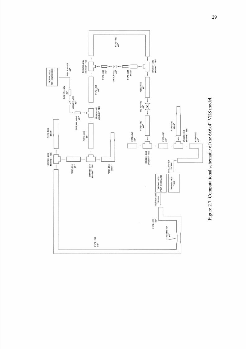
Figure 2.7. Computational schematic of the 6x6x4‖ VRS model..................................... 29
Figure 3.1. Experimental setup of the Void Recirculation System................................... 47
Figure 3.2. Lower pipe configurations used during the VRS experiment. ....................... 49
Figure 3.3. Sections of experimental interest for the Void Recirculation System. ........... 51
7/29/2019 Simulation and Validation of Two-component Flow in a Void Recircu
http://slidepdf.com/reader/full/simulation-and-validation-of-two-component-flow-in-a-void-recircu 12/171
xii
Figure 3.4. Horizontal stratified flow regime observed in the four and six-inch
pipes. ..................................................................................................................... 52
Figure 3.5. Downward bubbly flow regime observed in the four and six-inch
pipes. ..................................................................................................................... 54
Figure 3.6. Wavy horizontal stratified flow observed in the four and six-inch
pipes. ..................................................................................................................... 55
Figure 3.7 Bubbly and slug flow observed in the four and six-inch pipes. ...................... 56
Figure 3.8. Slug flow observed at station three in the four and six-inch pipes. ................ 57
Figure 3.9. Wavy horizontal stratified and bubbly flow transition observed at
station three in the four and six-inch pipes. .......................................................... 58
Figure 3.10. Bubbly flow observed at station four in the four and six-inch pipes. .......... 60
Figure 3.11. Upwards slug flow observed at the VRP for the four and six-inch
pipe configurations................................................................................................ 61
Figure 3.12. Upwards bubbly flow observed at the VRP for the four and six-inch
pipe configurations................................................................................................ 62
Figure 3.13. Taylor Bubble Train Flow Regime (Flow Regime Sample Movies). .......... 62
Figure 3.14. Air settling before the check valve in the six-inch branch. .......................... 64
Figure 3.15. Void fraction behavior for scenario one at station three for different
time steps. ............................................................................................................. 67
Figure 3.16. Void fraction behavior for scenario one at station three for different
mesh sizes. ............................................................................................................ 69
Figure 3.17. Mass flow rate behavior for simulation scenario one: 4x4x3-inch,
Fr = 0.81. .............................................................................................................. 75
7/29/2019 Simulation and Validation of Two-component Flow in a Void Recircu
http://slidepdf.com/reader/full/simulation-and-validation-of-two-component-flow-in-a-void-recircu 13/171
xiii
Figure 3.18. Mass flow rate and void fraction behavior at the recirculation pipe,
for simulation scenario one: 4x4x3-inch, Fr = 0.81. ............................................ 76
Figure 3.19. Mass flow rate and void fraction behavior at the recirculation pipe,
for simulation scenario eight: 6x6x4-inch, Fr = 1.60. .......................................... 78
Figure 3.20. Mass flow rate behavior for simulation scenario five: 6x6x4-inch,
Fr = 0.81. .............................................................................................................. 80
Figure 3.21. Void fraction behavior for simulation scenario one: 4x4x3-inch, Fr
= 0.81. ................................................................................................................... 83
Figure 3.22. Slip ratio and void fraction behavior at stations three and four, for
simulation scenario one: 4x4x3-inch, Fr = 0.81. .................................................. 86
Figure 3.23. Void fraction behavior for simulation scenario eight: 6x6x4-inch,
Fr = 1.60. .............................................................................................................. 89
Figure 3.24. Slip ratio and void fraction behavior at pipe section after lower
elbow, for simulation scenario one: 4x4x3-inch, Fr = 0.81.................................. 90
Figure 3.25. Slip ratio and void fraction behavior at pipe section after lower
elbow, for simulation scenario eight: 6x6x4-inch, Fr = 1.6. ................................ 91
Figure 3.26. Void fraction validation of the VRS model for simulation scenario
one: 4x4x3-inch, Fr = 0.81. .................................................................................. 93
Figure 3.27. Schematic of a pipe partially filled with water. ............................................ 94
Figure A.1. 4x4x3-inch VRS Pipe Configuration Drawing. .......................................... 102
Figure A.2. 6x6x4‖ VRS Pipe Configuration Drawing. ................................................ 103
Figure D.1. Mass flow rate behavior for scenario one (4x4x3-inch, Fr = 0.81)............. 144
Figure D.2. Mass flow rate behavior for scenario two (4x4x3-inch, Fr = 0.96). ........... 144

7/29/2019 Simulation and Validation of Two-component Flow in a Void Recircu
http://slidepdf.com/reader/full/simulation-and-validation-of-two-component-flow-in-a-void-recircu 14/171
xiv
Figure D.3. Mass flow rate behavior for scenario three (4x4x3-inch, Fr = 1.29). ......... 145
Figure D.4. Mass flow rate behavior for scenario four (4x4x3-inch, Fr = 1.60). ........... 145
Figure D.5. Mass flow rate behavior for scenario five (6x6x4-inch, Fr = 0.81). ........... 146
Figure D.6. Mass flow rate behavior for scenario six (6x6x4-inch, Fr = 1.10). ............. 146
Figure D.7. Mass flow rate behavior for scenario seven (6x6x4-inch, Fr = 1.38). ........ 147
Figure D.8. Mass flow rate behavior for scenario eight (6x6x4-inch, Fr = 1.60). ......... 147
Figure D.9. Void fraction behavior for scenario one (4x4x3-inch, Fr = 0.81). .............. 148
Figure D.10. Void fraction behavior for scenario two (4x4x3-inch, Fr = 0.96). ............ 148
Figure D.11. Void fraction behavior for scenario three (4x4x3-inch, Fr = 1.29). .......... 149
Figure D.12. Void fraction behavior for scenario four (4x4x3-inch, Fr = 1.60). ........... 149
Figure D.13. Void fraction behavior for scenario five (6x6x4-inch, Fr = 0.81). ........... 150
Figure D.14. Void fraction behavior for scenario six (6x6x4-inch, Fr = 1.10). ............. 150
Figure D.15. Void fraction behavior for scenario seven (6x6x4-inch, Fr = 1.38).......... 151
Figure D.16. Void fraction behavior for scenario eight (6x6x4-inch, Fr = 1.60). .......... 151
Figure E.1. Void fraction validation for scenario one (4x4x3-inch, Fr = 0.81). ............ 152
Figure E.2. Void fraction validation for scenario two (4x4x3-inch, Fr = 0.96). ............ 152
Figure E.3. Void fraction validation for scenario three (4x4x3-inch, Fr = 1.29). .......... 153
Figure E.4. Void fraction validation for scenario four (4x4x3-inch, Fr = 1.60). ........... 153
Figure E.5. Void fraction validation for scenario five (6x6x4-inch, Fr = 0.81). ............ 154
Figure E.6. Void fraction validation for scenario six (6x6x4-inch, Fr = 1.10). ............. 154
Figure E.7. Void fraction validation for scenario seven (6x6x4-inch, Fr = 1.38). ......... 155
Figure E.8. Void fraction validation for scenario eight (6x6x4-inch, Fr = 1.60). .......... 155
7/29/2019 Simulation and Validation of Two-component Flow in a Void Recircu
http://slidepdf.com/reader/full/simulation-and-validation-of-two-component-flow-in-a-void-recircu 15/171
xv
NOMENCLATURE
A Pipe cross-sectional area (ft )
C V Flow Coefficient
D Pipe Diameter (in)
Fr Froude Number
g Gravitational constant (ft/s )
j Fluid superficial velocity (ft/s)
K Loss coefficient
L Pipe length (ft) Mass flow rate (lb/s)
P Pressure (psi)
q Volumetric flow rate (gpm)
Re Reynolds number
S Slip ratio
t Time (s)
V Fluid velocity (ft/s)
x Flow quality
X Lockhart-Martinelli parameter
Z Volume centroid elevation (ft)
7/29/2019 Simulation and Validation of Two-component Flow in a Void Recircu
http://slidepdf.com/reader/full/simulation-and-validation-of-two-component-flow-in-a-void-recircu 16/171
xvi
Greek Characters
α Void fraction
θ Volume angle, measured from horizontal (degrees)
μ Fluid dynamic viscosity (lbf s/ft )
ρ Fluid density (slug/ft )
υ Fluid specific volume (ft /lb)
φ Two-phase multiplier
Subscripts
g Gas phase or component
i Interface between phases
k Phase or component (gas or liquid)
l Liquid phase or component
m Mixture
w Wall

7/29/2019 Simulation and Validation of Two-component Flow in a Void Recircu
http://slidepdf.com/reader/full/simulation-and-validation-of-two-component-flow-in-a-void-recircu 17/171
1
Chapter 1. INTRODUCTION AND LITERATURE REVIEW
1.1. Emergency Core Cooling System
Nuclear power plants rely on various protection systems that must be ready to
operate in case of a nuclear reactor failure. One of the most important protection plans is
the Emergency Core Cooling System (ECCS), which ultimately prevents a nuclear
meltdown by means of transferring heat from the reactor to the borated water, which is a
neutron absorber. When the ECCS is activated, borated water stored in a tank and
subject to atmospheric pressure, is pumped to the nuclear reactor as shown in Figure 1.1.
Figure 1.1. Schematic Diagram of the Emergency Core Cooling System. (Diablo Canyon
Power Plant, PG&E, 2009)
While this method has been used for many years and in many power plants, it has been
common to see dissolved gas being transported into the ECCS piping system. An
information notice from the Nuclear Regulatory Commission (NRC) was published
regarding the entrainment of gas into the ECCS and containment spray systems of three
main nuclear power plants (Nuclear Regulatory Commission, 2006). The source of
7/29/2019 Simulation and Validation of Two-component Flow in a Void Recircu
http://slidepdf.com/reader/full/simulation-and-validation-of-two-component-flow-in-a-void-recircu 18/171
2
entrained gas in these three events was due to different conditions, but produced the same
problem throughout. For example, NRC‘s inspection at Palo Verde Nuclear Generating
Station determined that gas was being entrained because the water level fell below the
suction piping. The second event described in the NRC‘s inspection was at the
Waterford Steam Electric Station, Unit 3, where it was determined that lack of
adjustments to the outside containment isolation valve led to loss of suction supply, thus
leading to a medium to large Loss of Coolant Accident (LOCA), creating large gas voids
within the suction piping. The last event described in this inspection was at the Clinton
Power Station, where it was determined that an inappropriate method was used to
calculate vortexing at the pump‘s intake. Another reason for the entrainment of gas into
ECCS piping systems, which is not discussed in this information notice from the NRC
and was specifically reported at the Diablo Canyon Power Plant (Avila Beach, CA), is a
consequence of the depressurization of the gas in the water tank. Gas depressurization
occurs when the local pressure falls below the saturation pressure of the gas. When this
happens, a water-gas flow is generated and later transported into the piping system
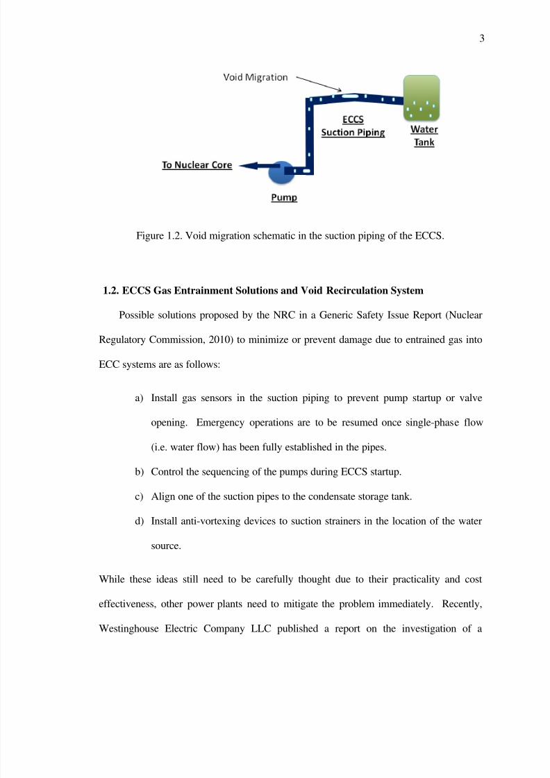
creating gas voids as specifically shown in Figure 1.2. Large voids in the suction side of
the pump can create cavitation, thus decreasing pump efficiency, lifetime, while adding
to the maintenance and repair costs. Even though some gas voids can be vented using
relief valves, other gas voids exist near the nuclear reactor where these types of valves
cannot be installed for safety purposes. For this reason, a series of solutions have been
proposed in the nuclear industry to minimize or eliminate the gas voids present in the
ECCS piping system. These solutions are discussed in the next section and are intended
to inform the reader about possible and existing solutions.
7/29/2019 Simulation and Validation of Two-component Flow in a Void Recircu
http://slidepdf.com/reader/full/simulation-and-validation-of-two-component-flow-in-a-void-recircu 19/171
3
Figure 1.2. Void migration schematic in the suction piping of the ECCS.
1.2. ECCS Gas Entrainment Solutions and Void Recirculation System
Possible solutions proposed by the NRC in a Generic Safety Issue Report (Nuclear
Regulatory Commission, 2010) to minimize or prevent damage due to entrained gas into
ECC systems are as follows:
a) Install gas sensors in the suction piping to prevent pump startup or valve
opening. Emergency operations are to be resumed once single-phase flow
(i.e. water flow) has been fully established in the pipes.
b) Control the sequencing of the pumps during ECCS startup.
c) Align one of the suction pipes to the condensate storage tank.
d) Install anti-vortexing devices to suction strainers in the location of the water
source.
While these ideas still need to be carefully thought due to their practicality and cost
effectiveness, other power plants need to mitigate the problem immediately. Recently,
Westinghouse Electric Company LLC published a report on the investigation of a
7/29/2019 Simulation and Validation of Two-component Flow in a Void Recircu
http://slidepdf.com/reader/full/simulation-and-validation-of-two-component-flow-in-a-void-recircu 20/171
4
simplified equation for gas transport in ECCS (Westinghouse Electric Company LLC,
2011). The simplified equation (SE) helps to find the maximum amount of gas volume in
pump suction piping, as a function of gas volume high points, system pressures and
flows. Even though the SE is based on a variety of assumptions and is limited to specific
pump suction piping configurations and flow regimes, it allows the ECCS to be activated
safely without risking pump damage. In fact, the Diablo Canyon Power Plant (DCPP)
has been one of the first plants to successfully use this SE, and is currently updating
safety procedures to keep the ECCS under normal operating conditions. In addition of
using the SE, DCPP has also been proactive at minimizing the amount of gas entrained
by installing a ―void header‖ that traps the air in a collector tank. Unfortunately, this tank
needs to be vented periodically by an operator, thus adding to the cost of labor and time.
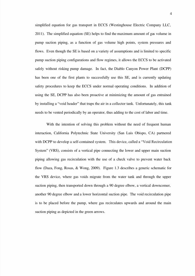
With the intention of solving this problem without the need of frequent human
interaction, California Polytechnic State University (San Luis Obispo, CA) partnered
with DCPP to develop a self-contained system. This device, called a ―Void Recirculation
System‖ (VRS), consists of a vertical pipe connecting the lower and upper main suction
piping allowing gas recirculation with the use of a check valve to prevent water back
flow (Daza, Fong, Rosas, & Wong, 2009). Figure 1.3 describes a generic schematic for
the VRS device, where gas voids migrate from the water tank and through the upper
suction piping, then transported down through a 90 degree elbow, a vertical downcomer,
another 90 degree elbow and a lower horizontal suction pipe. The void recirculation pipe
is to be placed before the pump, where gas recirculates upwards and around the main
suction piping as depicted in the green arrows.

7/29/2019 Simulation and Validation of Two-component Flow in a Void Recircu
http://slidepdf.com/reader/full/simulation-and-validation-of-two-component-flow-in-a-void-recircu 21/171
5
Figure 1.3. Generic schematic of the Void Recirculation System device to be used in the
ECCS.
This device was tested under different flow rates, initial void quantities, and bottom pipe
configurations. Air was injected in the system by using an air compressor and the VRS
was tested on the discharge side of the pump, rather than on the suction side, for the sake
of the experiment. Void fraction measurements were taken at stations one (before the
upper tee), two (after the upper tee), three (before the lower tee) and four (after the lower
tee). The objective of this experiment was to verify the design of the VRS and to select
the best bottom piping configuration for each of the tested scenarios. The data recorded
from this experiment will be used in this thesis to validate the VRS concept using a
thermal-hydraulic computer code called RELAP5/Mod3.
1.3. Review of existing ECCS models
There are several investigators who have modeled a variety of scenarios in ECCS
and have contributed to the analysis and prediction of LOCAs. The main objective in

7/29/2019 Simulation and Validation of Two-component Flow in a Void Recircu
http://slidepdf.com/reader/full/simulation-and-validation-of-two-component-flow-in-a-void-recircu 22/171
6
these contributions is to provide better management and operating procedures in case of
nuclear accidents. Sarrette and Bestion, for example, investigated the potential release of
nitrogen gas dissolved in water during depressurization in the accumulator of the ECCS
at the Loviisa Nuclear Power Plant (Sarrette & Bestion, 2003). The first part of their
work consisted of performing a series of degassing tests in order to find the time constant
associated with the nitrogen gas release in a vertical pipe. Then, a non-condensable gas
dissolution-release model was created using CATHARE (Code Avancé de
Thermohydraulique pour Accidents de Réacteur à Eau), a thermal-hydraulic code for the
nuclear safety analysis of Pressurized Water Reactors (PWR). An interfacial friction
model consistent with the flow configuration seen in the experimental results, along with
the gas-release time constant previously found, was later implemented in CATHARE.
Finally, the code was used to investigate the effects of nitrogen degassing for LOCA
scenarios. Numerical results showed better agreement with experimental results for the
case of delayed degassing than for faster degassing.
A similar work at DCPP, where the effect of nitrogen gas entrained was studied in
ECCS piping systems, was the effort done by Phillips in his water hammer simulation
using RELAP5 (Phillips, 2003). During the pump startup operation, pressure waves can
be generated if gas voids are present in the piping system. This effect, commonly known
as a water hammer, can create high pipe stresses in elbows due to rapid change in
direction, thus leading to pipe damage and possible ECCS failure. Pipe stresses modeled
in RELAP5, measured as hydraulic forces, were subject to 100% and 50% void models in
order to fully analyze the water hammer effect. Even though the model provided a
7/29/2019 Simulation and Validation of Two-component Flow in a Void Recircu
http://slidepdf.com/reader/full/simulation-and-validation-of-two-component-flow-in-a-void-recircu 23/171
7
reasonable prediction of hydraulic forces, the maximum calculated values continue to be
under the safety order of magnitude during a LOCA.
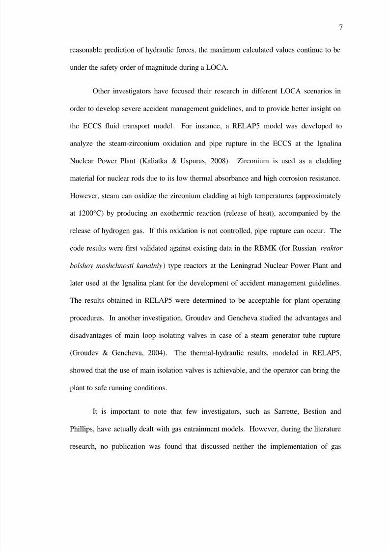
Other investigators have focused their research in different LOCA scenarios in
order to develop severe accident management guidelines, and to provide better insight on
the ECCS fluid transport model. For instance, a RELAP5 model was developed to
analyze the steam-zirconium oxidation and pipe rupture in the ECCS at the Ignalina
Nuclear Power Plant (Kaliatka & Uspuras, 2008). Zirconium is used as a cladding
material for nuclear rods due to its low thermal absorbance and high corrosion resistance.
However, steam can oxidize the zirconium cladding at high temperatures (approximately
at 1200°C) by producing an exothermic reaction (release of heat), accompanied by the
release of hydrogen gas. If this oxidation is not controlled, pipe rupture can occur. The
code results were first validated against existing data in the RBMK (for Russian reaktor
bolshoy moshchnosti kanalniy) type reactors at the Leningrad Nuclear Power Plant and
later used at the Ignalina plant for the development of accident management guidelines.
The results obtained in RELAP5 were determined to be acceptable for plant operating
procedures. In another investigation, Groudev and Gencheva studied the advantages and
disadvantages of main loop isolating valves in case of a steam generator tube rupture
(Groudev & Gencheva, 2004). The thermal-hydraulic results, modeled in RELAP5,
showed that the use of main isolation valves is achievable, and the operator can bring the
plant to safe running conditions.
It is important to note that few investigators, such as Sarrette, Bestion and
Phillips, have actually dealt with gas entrainment models. However, during the literature
research, no publication was found that discussed neither the implementation of gas

7/29/2019 Simulation and Validation of Two-component Flow in a Void Recircu
http://slidepdf.com/reader/full/simulation-and-validation-of-two-component-flow-in-a-void-recircu 24/171
8
entrainment solutions nor the modeling of possible solutions in ECCS piping systems.
For this reason, the motivation of using RELAP5/MOD3 to build a computational model,
representing the experimental setup of the VRS, was initiated to simulate gas entrainment
solutions in ECCS. The numerical results obtained were used to evaluate the practicality
of one of the first gas entrainment solutions, and were validated against the results
obtained from the VRS experiment. This one involves the subject of two-phase flow in
pipes, for which a literature review of these models will be discussed in the next section.
1.4. Review of existing Two-Phase flow models
Since the VRS experiment mainly focused on the void fraction behavior at the
upper and lower main pipes, and not the effects that elbows had on the recirculation path,
the following literature research also focuses on two-phase horizontal flows and flow
separation at tee junctions. Moreover, the research will be limited to horizontal stratified
flows since this was the flow regime that was observed during the VRS experiments.
The investigation and analysis of two-phase flows has been carried out by
numerous researchers depending upon the conditions of interest. The contributions done
by Ishii and Mishima have been of great value to the multi-phase community because
they have formalized all equations to be used for mass, momentum and energy
conservation (Ishii, 1975; Ishii & Mishima, 1984). Other researchers such as Taitel,
Dukler and Chisholm have also contributed to this immense field by providing theoretical
approaches to the prediction of pressure drop in pipelines (Taitel & Dukler, 1976;
Chisholm, 1968).

7/29/2019 Simulation and Validation of Two-component Flow in a Void Recircu
http://slidepdf.com/reader/full/simulation-and-validation-of-two-component-flow-in-a-void-recircu 25/171
9
With the introducton of today‘s powerful computational techniques, it has been
possible to better predict many variables of interest for two-phase flow (e.g. void fraction,
pressure drop, flow regimes, etc.). For instance, Newton and Behnia (2001) developed a
numerical model for horizontal stratified wavy gas-liquid pipe flow, that predicted liquid
holdup, pressure drop, wall and interfacial shear stresses. The main objective of this
numerical model was to gain independence of empirical closure relations, by providing a
bipolar coordinate system, along with a turbulunce model at low Reynolds
numbers, allowing the solution of the governing equations for each phase without
inputting empirical wall functions. The proposed numerical model was then compared to
existing mechanisitc models, and the prediction of the measured values were in
acceptable agreement with the experimental data. In a similar investigation, a model was
proposed using the Reynolds-averaged Navier-Stokes (RANS) equations, with the
turbulence model for fully developed horizontal stratified flow in pipes (de Sampaio,
Faccini, & Su, 2008). This model used a finite element mesh, bipolar coordinates, the
Newton-Raphson root finding scheme, and focused on simulating the wall and interfacial
shear stresses to provide better insight on the interaction of gas-liquid flows, with the
objective of validating the use of the turbulence model. The predicted values were
then compared to experimental data, showing that the turbulence model was suitable for
horizontal stratified flows. Yet another numerical simulation was carried out using
FLUENT to deterimine the interfacial friction factor for horizontal stratified gas-liquid
3D flows (Sidi-Ali & Gatignol, 2010). Velocity profiles, wall-gas shear stresses and
interfacial shear stresses numerical results were compared to seven different experiments
and one numerical model. The results comparison showed to be in excellent agreement

7/29/2019 Simulation and Validation of Two-component Flow in a Void Recircu
http://slidepdf.com/reader/full/simulation-and-validation-of-two-component-flow-in-a-void-recircu 26/171
10
for velocity profiles, and acceptable agreement for wall-gas and interfacial shear stresses,
confirming the validity of the turbulence model used.
Simulation of the bottom horizontal tee for the VRS experiment can be seen as a
form of two-phase separator, with the exception that the gas recirculation path is actually
connected to the same main pipe loop. The orientation of the tee, where there is a
horizontal run and a vertical branch (with upwards flow), is of particular interest for the
validation of the VRS device and hence the computational model presented in this thesis.
In the attempt of analyzing this specific type of flow configuration, Margaris (2007)
proposed a mathematical algorithm to model the separation of gas-liquid two-phase flow
at a tee junction. The experimental and numerical models both assumed a horizontal
straight pipe before the tee junction with slug flow at the tee inlet, the air was separated
through the vertical branch and the water continued its path through the horizontal run.
The vertical branch then connected to a horizontal settling pipe, where further separation
was allowed. The air continued its path into an independent gas line, and the water fell
downwards into the lower main horizontal pipeline through a vertical pipe. Air and water
mass flow rates were compared, as well as void fraction and pressure drop at the tee
junction and at the settling pipe. The numerical results obtained showed satisfactory
results with respect to the experimental data, and the mathematical algorithm was
successfully validated. Margaris also suggested the implementation of this algorithm into
other computer codes due to its easy incorporation of one-dimensional multiphase flow.
Other similar investigations carried out by Ottens et al. (2001) and Baker et al. (2008),
studied the transient effects in gas-liquid separators by using different pipe configurations
and tee orientations. Nonetheless, the experiments carried out in both works showed that
7/29/2019 Simulation and Validation of Two-component Flow in a Void Recircu
http://slidepdf.com/reader/full/simulation-and-validation-of-two-component-flow-in-a-void-recircu 27/171
11
the different phases were completely separated in different pipelines, as was the case for
the research done by Margaris.
1.5. Computational Tool
Numerical simulations for nuclear power plant systems can be done in a variety of
computational fluid dynamic (CFD) solvers depending upon the specific problem to be
analyzed. Software such as FLUENT (by ANSYS), SolidWorks Flow Simulation and
Flow-3D could potentially be used to solve two-phase flow simulation problems. The
software selection mainly depends on the computational domain to be solved, being
either a small subsystem (e.g. flow around an object), or the analysis of a complete
system (e.g. power plant thermal and hydraulic systems). Since this thesis analyzes air-
water flow in nuclear power plant pipelines that change both in diameter and orientation,
then the current study will use RELAP5/MOD3 to simulate the VRS device.
RELAP5 stands for Reactor Excursion and Leak Analysis Program, and is the
fifth version of all RELAP codes. It is a thermal/hydraulic computer code developed for
the U.S. NRC for the use of rulemaking, operating guidelines and as nuclear plant
analyzer. Hence, it is the only code accepted by the NRC if simulation data is to be
presented in any form of publication. In addition, DCPP uses this code to analyze the
plant, and the code developed in this study can potentially be used at their site for further
development. RELAP5 computer code is written in FORTRAN 77 and uses one-
dimensional two-fluid conservation equations that are formulated in terms of volume and

7/29/2019 Simulation and Validation of Two-component Flow in a Void Recircu
http://slidepdf.com/reader/full/simulation-and-validation-of-two-component-flow-in-a-void-recircu 28/171
12
time-averaged parameters. The code also uses a semi-implicit finite-difference technique
to solve the computational domain and is first-order accurate in space and time.
1.5.1. RELAP5/MOD3 Applications
The computer code RELAP, being in its fifth version, has a variety of co-current
and new models that are used to simulate and analyze specific nuclear plant systems such
as steady-state and transient problems, Emergency Core Cooling mixing component
model, Zirconium-water reaction model, correlations for interfacial friction in all
geometries, an improved cross flow model and many more (RELAP5/MOD3.2, Code
Manual Volume I: Code Structure, System Models, and Solution Methods, 1995). In
general, RELAP5 is commonly used to simulate LOCA‘s, loss of feed-water, station
blackout and turbine trip. It can also be used to simulate mixtures of steam, water, and
non-condensable gases.
1.5.2. RELAP5/MOD3 Limitations
As previously mentioned, it is wise to carefully choose the CFD tool to be used
for each problem since not all software is capable of analyzing an entire scope of
computational domains. In the case of RELAP5, the code has two main limitations that
were depicted during the learning phase of the program. First, the code cannot be used to
analyze flows around objects. For example, the analysis of variables such as pressure and
temperature gradients, streamlines, and velocities cannot be done on the problem of flow
through an orifice. Second, the process of nodalization is limited to the L / D ratio ( L is

7/29/2019 Simulation and Validation of Two-component Flow in a Void Recircu
http://slidepdf.com/reader/full/simulation-and-validation-of-two-component-flow-in-a-void-recircu 29/171
13
the volume length and D is the volume diameter) for numerical stability. There are other
limitations depending upon the models to be used within the program, and is strongly
suggested to review the components to be used, along with their limitations, before
deciding to use RELAP5.
1.6. Objectives
The objectives of this thesis are to (1) simulate and investigate two-component
air-water flow in a void recirculation system that minimizes the amount of air in piping
systems, using RELAP5/MOD3 as the computational tool, and (2) to validate the
numerical results obtained from the void recirculation system model with respect to
experimental results and observations.
The objectives previously mentioned will be approached in Chapter 2, where the
computational model is explained from both the theoretical and geometrical viewpoints;
and in Chapter 3, where the results from the model are discussed and validated against
experimental results. Chapter 4 highlights the most significant achievements of this work
and provides recommendations for future work.

7/29/2019 Simulation and Validation of Two-component Flow in a Void Recircu
http://slidepdf.com/reader/full/simulation-and-validation-of-two-component-flow-in-a-void-recircu 30/171
14
Chapter 2. COMPUTATIONAL MODEL
2.1. Two-Fluid General Definitions
The two-fluid flow model used in RELAP5, which will be discussed in the next
section, requires the definition of unique parameters that are pertinent to this field of
study. It is important to note that there are several parameters used in two-fluid flow, but
only the concepts of interest will be defined.
2.1.1. Froude Number
The Froude number is a dimensionless parameter representing the ratio of inertia
to gravitational forces. In general, it can be applied to open-channel flow (Jain, 2001),
where the free surface of the water is subject to atmospheric pressure; and in pipe flow,
where gaseous and liquid phases interact with each other (i.e. two-fluid flow). The
Froude number equation is as follows:
(2.1)
where V l represents the liquid velocity, ρl the liquid density, ρg the gas density, g the
gravitational constant and D the inside pipe diameter. Because ρl >> ρg, for the case of
water and air as the main working fluids, then:
(2.2)

7/29/2019 Simulation and Validation of Two-component Flow in a Void Recircu
http://slidepdf.com/reader/full/simulation-and-validation-of-two-component-flow-in-a-void-recircu 31/171
15
The Froude number categorizes the flow in three main regimes: Fr < 1 for subcritical
flow, Fr = 1 for critical flow and Fr > 1 for supercritical flow (Fox, McDonald, &
Pritchard, 2006). Previous works, for example, analyzed the influence of the Froude
number in determining the frequency at which air-water horizontal slug flow occurs
(Woods & Hanratty, 1999). In this analysis, it was determined that Froude numbers less
than unity led to gravity waves upstream, caused by the formation of slug flows. In a
similar example, the Froude number was used to characterize and predict the transition
from horizontal stratified to slug flow (Kadri, Mudde, Oliemans, Bonizzi, & Andreussi,
2009). Because of the Froude number significance in the industry, this paper will use the
parameter in discussion for flow regime predictions and void fraction calculations.
Other basic parameters used in two-fluid flow are void fraction, superficial
velocity, slip ratio and flow quality (Ghiaasiaan, 2008). These will be discussed in more
detail in the following sections, will be used in different models and correlations, and
assume the form of composite-averaged parameters.
2.1.2. Void Fraction
The void fraction can be defined as the ratio of the area occupied by the gas to the
total cross-sectional area as follows:
(2.3)
where Ag is the area occupied by the gas and A is the total cross-sectional area of the pipe.
7/29/2019 Simulation and Validation of Two-component Flow in a Void Recircu
http://slidepdf.com/reader/full/simulation-and-validation-of-two-component-flow-in-a-void-recircu 32/171
16
2.1.3. Superficial Velocity
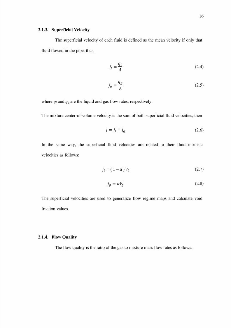
The superficial velocity of each fluid is defined as the mean velocity if only that
fluid flowed in the pipe, thus,
(2.4)
(2.5)
where ql and qg are the liquid and gas flow rates, respectively.
The mixture center-of-volume velocity is the sum of both superficial fluid velocities, then
(2.6)
In the same way, the superficial fluid velocities are related to their fluid intrinsic
velocities as follows:
(2.7)
(2.8)
The superficial velocities are used to generalize flow regime maps and calculate void
fraction values.
2.1.4. Flow Quality
The flow quality is the ratio of the gas to mixture mass flow rates as follows:
7/29/2019 Simulation and Validation of Two-component Flow in a Void Recircu
http://slidepdf.com/reader/full/simulation-and-validation-of-two-component-flow-in-a-void-recircu 33/171
17
(2.9)
where
and
represent the gas and liquid mass flow rates, respectively. This
parameter will also be used to calculate both void fraction and two-fluid pressure drop
values.
2.1.5. Slip Ratio
The slip ratio is a relationship between the gas and liquid velocities that allows
describing velocity differences between the phases or components as follows:
(2.10)
The slip ratio has a direct and indirect proportional relationship with the gas and liquid
velocities, respectively. More specifically, as the gas velocity decreases, the slip ratio
decreases as well, implying that the gaseous phase or component moves slower than the
liquid component. This parameter will be used to validate numerical results.
2.2. Two-Fluid Flow Model used in RELAP5
Two-fluid flow is concerned with the simultaneous flow of two fluids in a given
space. It can occur in many industrial applications such as boiling and pressurized water
reactors, evaporators, condensers, jet pumps and many more. This concept can be
divided into two subcategories for which they are well known in the industry (Wallis,
1969):
7/29/2019 Simulation and Validation of Two-component Flow in a Void Recircu
http://slidepdf.com/reader/full/simulation-and-validation-of-two-component-flow-in-a-void-recircu 34/171
18
1. Two-Phase flow, in which the fluids can be of the same component but of
different states of matter, such as gas, liquid or solid.
2. Two-Component flow, in which the fluids do not consist of the same chemical
substance, such as water and air.
These three terms will be used interchangeably throughout this paper depending on the
matters to be discussed, but all mathematical notions and derivations are identical.
Another term used in different references, and which will not be discussed in this paper,
is Multi-Phase flow, which concerns the simultaneous flow of more than two phases or
components.
2.2.1. One-Dimensional Two-Fluid Conservation Equations
Two-fluid flows follow the same laws as those described in fluid dynamics, and in
fact are derived from single-phase or single-fluid conservation equations, though they are
more complex and numerous since more variables have to be accounted for. The basic
field one-dimensional equations for the two-fluid model consists of two continuity
equations, two momentum equations and two energy equations as follows
(RELAP5/MOD3.2, Code Manual Volume I: Code Structure, System Models, and
Solution Methods, 1995):
Continuity Equation:
(2.11)

7/29/2019 Simulation and Validation of Two-component Flow in a Void Recircu
http://slidepdf.com/reader/full/simulation-and-validation-of-two-component-flow-in-a-void-recircu 35/171
19
where the subscript k denotes the phase or component of interest, that is k = g for the gas
phase and k = l for the liquid phase; and is the gas or liquid generation depending on
the phase of interest.
Momentum Equation:
(2.12)
where the subscript i is the interface between the phases, j is the opposite phase of
interest, and m represents the flow mixture. Also,
P = Pressure
B = Body force (i.e. gravity and pump head)
FW = Wall frictional drag coefficient
FI = Interface frictional drag coefficient
C = Virtual mass coefficient
7/29/2019 Simulation and Validation of Two-component Flow in a Void Recircu
http://slidepdf.com/reader/full/simulation-and-validation-of-two-component-flow-in-a-void-recircu 36/171
20
Energy Equation:
(2.13)
where,
U = Specific internal energy
= Phasic wall heat transfer
= Interfacial heat transfer
= Phasic enthalpy associated with bulk interface mass transfer
= Phasic enthalpy associated with wall interface mass transfer
DISS = Phasic energy dissipation (sums of wall friction and pump effects)
2.2.2. Flow Regimes
Two-phase flow patterns or regimes can occur in many ways depending upon
volume orientation, diameter, flow rates, fluid density, fluid viscosity, surface tension,
and other parameters. The main flow regimes seen in horizontal flow are bubbly, plug,
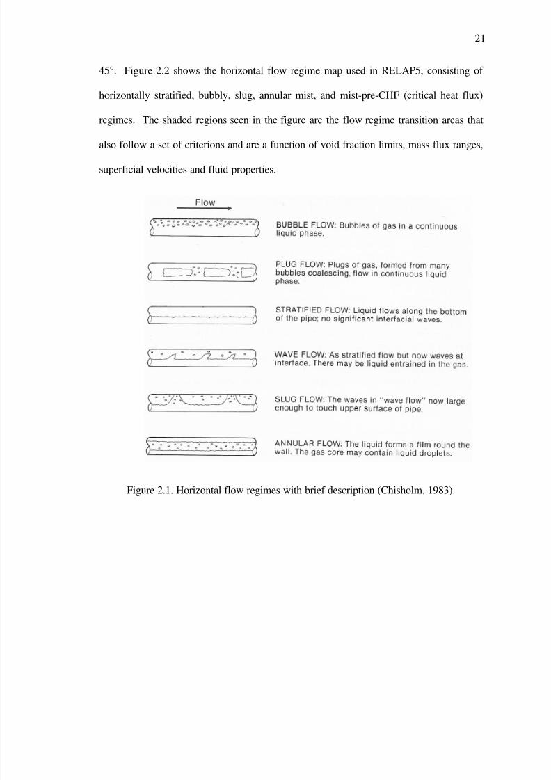
stratified, stratified-wavy, slug and annular flow (Chisholm, 1983). Figure 2.1 briefly
describes the most common horizontal flow regimes seen in two-phase flow. The
regimes are organized in ascending gas flow rates such that bubbly flow has the lowest
gas flow rate, and annular flow has the highest gas flow rate. In order to determine the
type of flow regime, RELAP5 uses a specific horizontal flow regime map that is based on
several empirical correlations, and only applies to volume orientations between 0° and
7/29/2019 Simulation and Validation of Two-component Flow in a Void Recircu
http://slidepdf.com/reader/full/simulation-and-validation-of-two-component-flow-in-a-void-recircu 37/171
21
45°. Figure 2.2 shows the horizontal flow regime map used in RELAP5, consisting of
horizontally stratified, bubbly, slug, annular mist, and mist-pre-CHF (critical heat flux)
regimes. The shaded regions seen in the figure are the flow regime transition areas that
also follow a set of criterions and are a function of void fraction limits, mass flux ranges,
superficial velocities and fluid properties.
Figure 2.1. Horizontal flow regimes with brief description (Chisholm, 1983).
7/29/2019 Simulation and Validation of Two-component Flow in a Void Recircu
http://slidepdf.com/reader/full/simulation-and-validation-of-two-component-flow-in-a-void-recircu 38/171
22
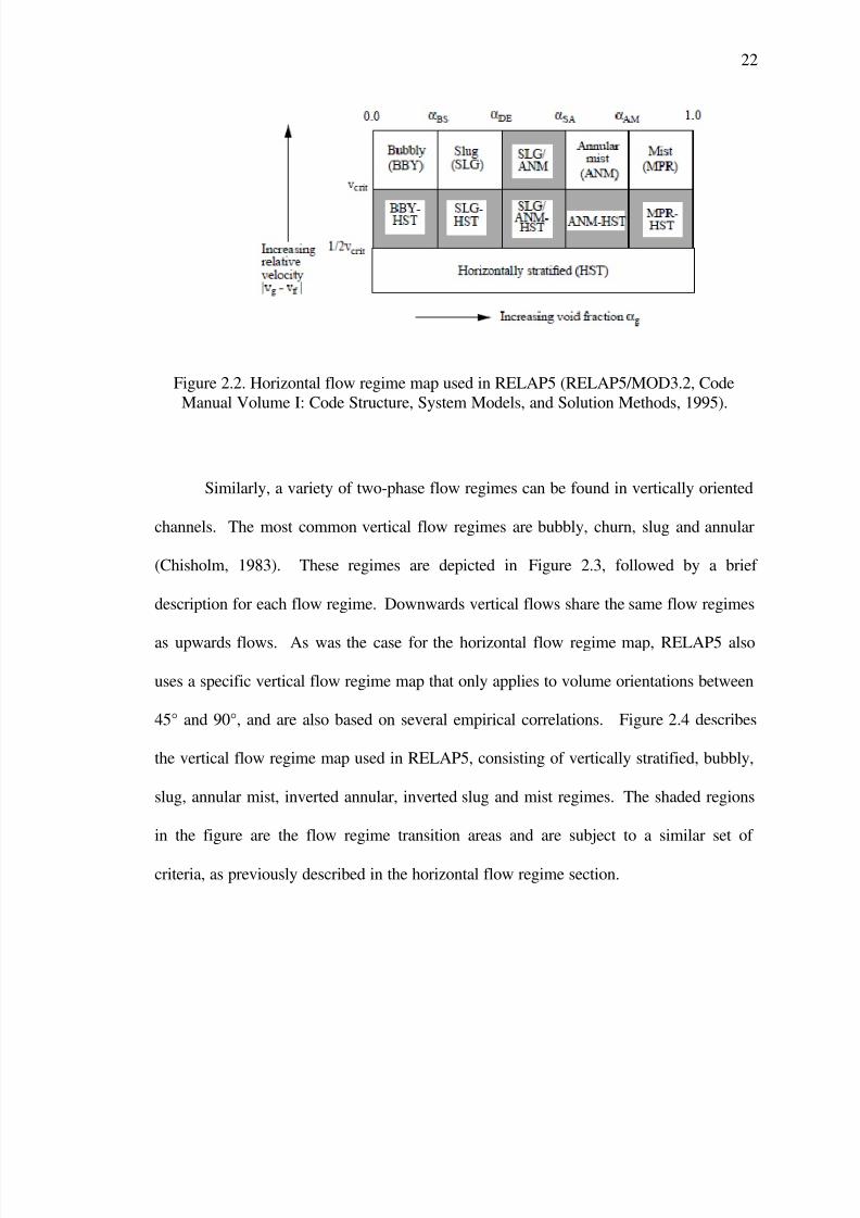
Figure 2.2. Horizontal flow regime map used in RELAP5 (RELAP5/MOD3.2, Code
Manual Volume I: Code Structure, System Models, and Solution Methods, 1995).
Similarly, a variety of two-phase flow regimes can be found in vertically oriented
channels. The most common vertical flow regimes are bubbly, churn, slug and annular
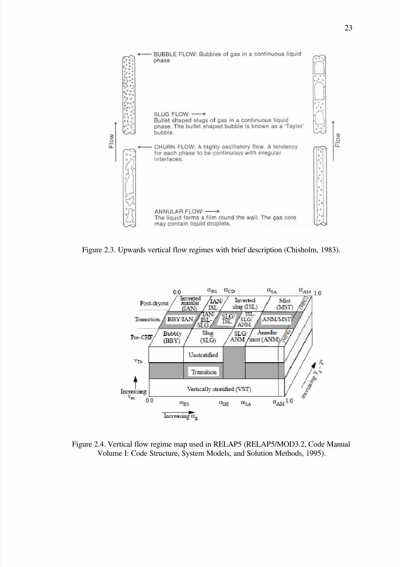
(Chisholm, 1983). These regimes are depicted in Figure 2.3, followed by a brief
description for each flow regime. Downwards vertical flows share the same flow regimes
as upwards flows. As was the case for the horizontal flow regime map, RELAP5 also
uses a specific vertical flow regime map that only applies to volume orientations between
45° and 90°, and are also based on several empirical correlations. Figure 2.4 describes
the vertical flow regime map used in RELAP5, consisting of vertically stratified, bubbly,
slug, annular mist, inverted annular, inverted slug and mist regimes. The shaded regions
in the figure are the flow regime transition areas and are subject to a similar set of
criteria, as previously described in the horizontal flow regime section.
7/29/2019 Simulation and Validation of Two-component Flow in a Void Recircu
http://slidepdf.com/reader/full/simulation-and-validation-of-two-component-flow-in-a-void-recircu 39/171
23
Figure 2.3. Upwards vertical flow regimes with brief description (Chisholm, 1983).
Figure 2.4. Vertical flow regime map used in RELAP5 (RELAP5/MOD3.2, Code Manual
Volume I: Code Structure, System Models, and Solution Methods, 1995).

7/29/2019 Simulation and Validation of Two-component Flow in a Void Recircu
http://slidepdf.com/reader/full/simulation-and-validation-of-two-component-flow-in-a-void-recircu 40/171
24
2.2.3. Wall Friction Model
The wall friction calculated in RELAP5 is based on the flow regime maps
previously discussed, in that each flow regime provides a criterion to determine the wall
friction for each phase. It is essential to note that only wall shear effects are included,
losses due to enlargement and contraction devices are calculated using mechanistic
models, and losses due to elbows are modeled using flow loss coefficients that must be
input by the code user.
The wall friction model is based on the two-phase multiplier approach, where the
Heat Transfer and Fluid Flow Service (HTFS)-modified Baroczy correlation
(RELAP5/MOD3.2, Code Manual Volume I: Code Structure, System Models, and
Solution Methods, 1995) is used to find the two-phase multiplier. The total friction
pressure drop in terms of the pure phasic wall friction pressure drop is
(2.14)
where is the pure phase (fluid or gas) two-phase multiplier, and is short for two-
phase. The phasic wall friction pressure gradient is as follows:
(2.15)
where λ is the single-phase friction factor, the prime denotes the pure liquid or pure gas
condition, and is the Reynolds number defined as
(2.16)

7/29/2019 Simulation and Validation of Two-component Flow in a Void Recircu
http://slidepdf.com/reader/full/simulation-and-validation-of-two-component-flow-in-a-void-recircu 41/171
25
where is the dynamic viscosity. The mass flow rate as a function of phasic void
fraction, density, velocity and area can be expressed as
(2.17)
Finally, the Lockhart-Martinelli parameter can be defined as the ratio of the pure two-
phase multipliers, and are related to their pure phasic wall pressure drop as follows:
(2.18)
The respective pure liquid and gas two-phase multipliers can be found by using the
HTFS-modified Baroczy correlation:
(2.19)
(2.20)
where C is the correlation coefficient and is a function of the scalar mass flux and other
dimensionless parameters (RELAP5/MOD3.2, Code Manual Volume I: Code Structure,
System Models, and Solution Methods, 1995).

7/29/2019 Simulation and Validation of Two-component Flow in a Void Recircu
http://slidepdf.com/reader/full/simulation-and-validation-of-two-component-flow-in-a-void-recircu 42/171
26
2.3. Computational Domain
2.3.1. VRS Model Geometry
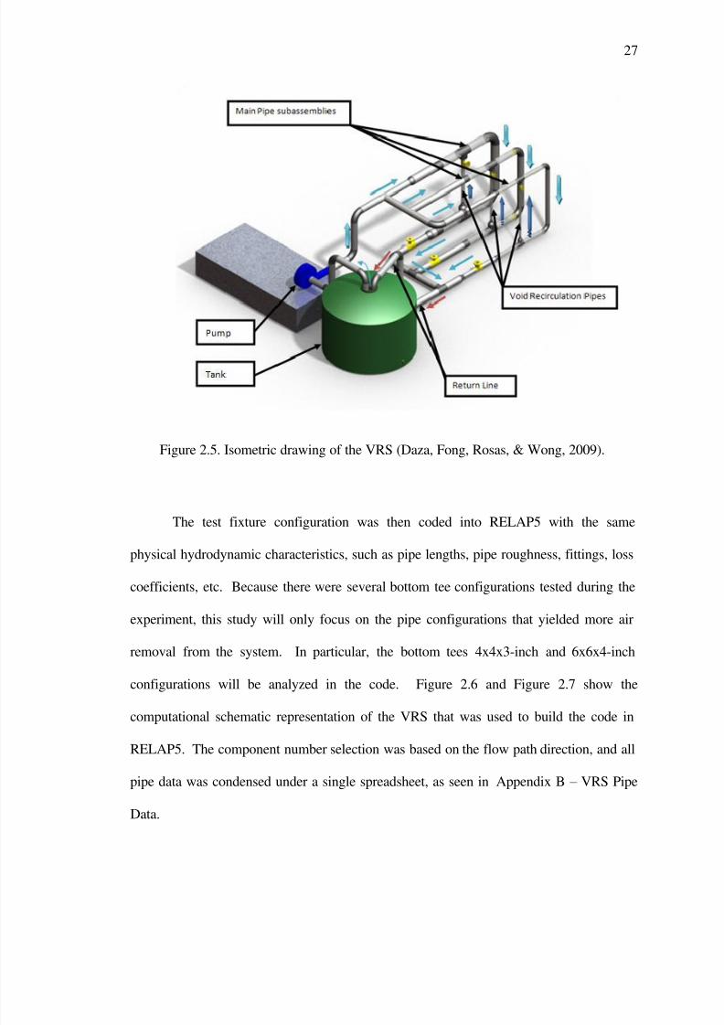
The computational domain analyzed in this study was based on the experimental
fixture of the VRS, which can be fully appreciated in Figure 2.5. The test fixture
consisted of a 1000 gallon tank, a six-inch trash pump and three main pipe
subassemblies: four-inch, six-inch and eight-inch. Due to the limited air injection power
available to the project, the eight-inch pipe was not able to be tested with the initial
amount of void fraction requested by DCPP. For this reason, only the four and six-inch
pipe subassemblies were able to be tested, which are consequently the experimental
scenarios to be modeled in RELAP5. The flow path starts at the tank, where the pump is
drawing water through the six-inch suction pipe and later discharged to the main six-inch
pipe. The flow path is then directed upwards where it is divided into three main pipe
subassemblies or branches. Only one main branch is allowed to operate during the
experiment by opening the ball valve that corresponds to the branch of interest. The flow
path then continues through the main branch until it encounters the main return line,
which ultimately leads to the same tank. Air was injected with a two-horsepower, 33
gallon, 150 maximum psi compressor, at locations before the upper tee.
7/29/2019 Simulation and Validation of Two-component Flow in a Void Recircu
http://slidepdf.com/reader/full/simulation-and-validation-of-two-component-flow-in-a-void-recircu 43/171
27
Figure 2.5. Isometric drawing of the VRS (Daza, Fong, Rosas, & Wong, 2009).
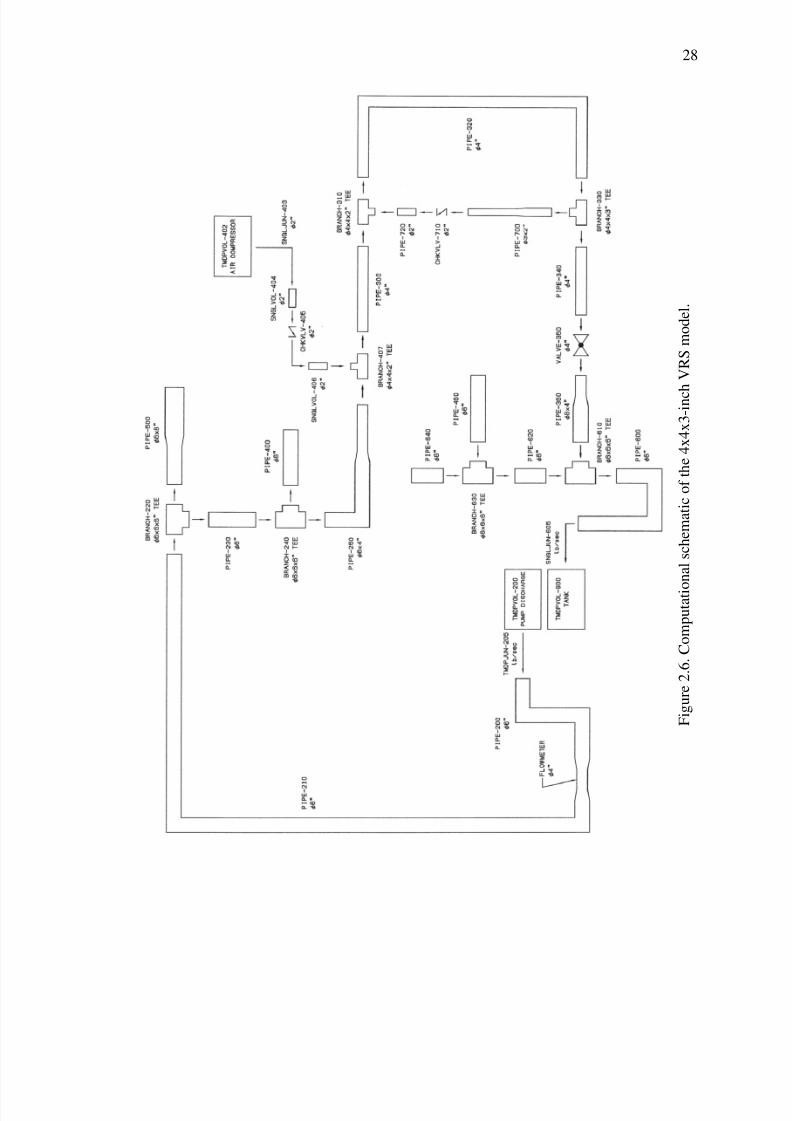
The test fixture configuration was then coded into RELAP5 with the same
physical hydrodynamic characteristics, such as pipe lengths, pipe roughness, fittings, loss
coefficients, etc. Because there were several bottom tee configurations tested during the
experiment, this study will only focus on the pipe configurations that yielded more air
removal from the system. In particular, the bottom tees 4x4x3-inch and 6x6x4-inch
configurations will be analyzed in the code. Figure 2.6 and Figure 2.7 show the
computational schematic representation of the VRS that was used to build the code in
RELAP5. The component number selection was based on the flow path direction, and all
pipe data was condensed under a single spreadsheet, as seen in Appendix B – VRS Pipe
Data.
7/29/2019 Simulation and Validation of Two-component Flow in a Void Recircu
http://slidepdf.com/reader/full/simulation-and-validation-of-two-component-flow-in-a-void-recircu 44/171
28
F i g u r e 2 . 6 . C o m p u t a t i o
n a l s c h e m a t i c o f t h e 4 x 4 x 3 - i n c h V R S m o d e l .
7/29/2019 Simulation and Validation of Two-component Flow in a Void Recircu
http://slidepdf.com/reader/full/simulation-and-validation-of-two-component-flow-in-a-void-recircu 45/171
29
F i g u r e 2 . 7 . C o m p u t a t i o n a l s c h e m a t i c o f t h e 6 x 6 x 4 ‖
V R S m o d e l .
7/29/2019 Simulation and Validation of Two-component Flow in a Void Recircu
http://slidepdf.com/reader/full/simulation-and-validation-of-two-component-flow-in-a-void-recircu 46/171
30
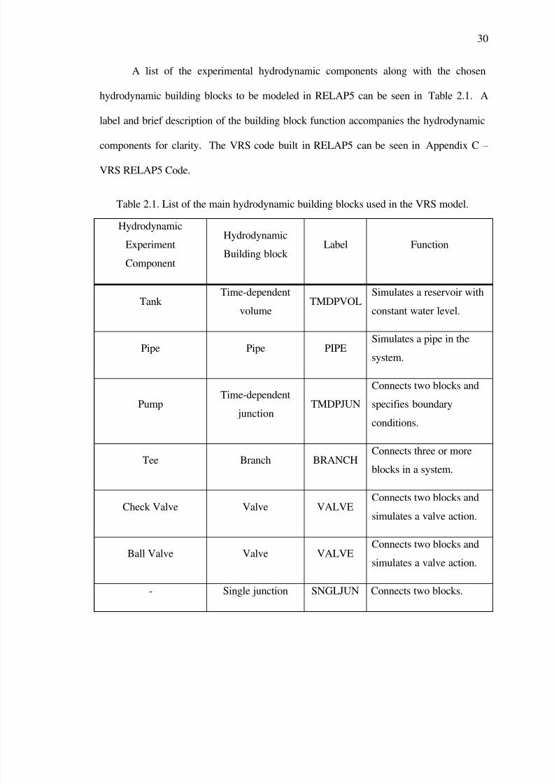
A list of the experimental hydrodynamic components along with the chosen
hydrodynamic building blocks to be modeled in RELAP5 can be seen in Table 2.1. A
label and brief description of the building block function accompanies the hydrodynamic
components for clarity. The VRS code built in RELAP5 can be seen in Appendix C –
VRS RELAP5 Code.
Table 2.1. List of the main hydrodynamic building blocks used in the VRS model.
Hydrodynamic
Experiment
Component
Hydrodynamic
Building block Label Function
Tank Time-dependent
volumeTMDPVOL
Simulates a reservoir with
constant water level.
Pipe Pipe PIPESimulates a pipe in the
system.
PumpTime-dependent
junctionTMDPJUN
Connects two blocks and
specifies boundary
conditions.
Tee Branch BRANCHConnects three or more
blocks in a system.
Check Valve Valve VALVEConnects two blocks and
simulates a valve action.
Ball Valve Valve VALVE Connects two blocks andsimulates a valve action.
- Single junction SNGLJUN Connects two blocks.
7/29/2019 Simulation and Validation of Two-component Flow in a Void Recircu
http://slidepdf.com/reader/full/simulation-and-validation-of-two-component-flow-in-a-void-recircu 47/171
31
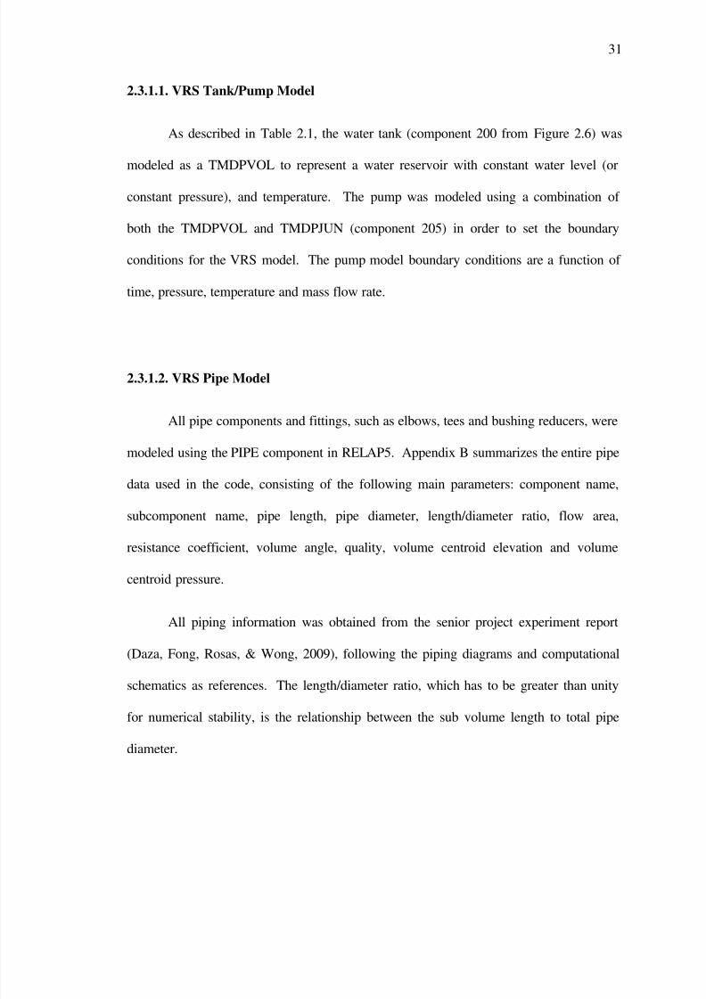
2.3.1.1. VRS Tank/Pump Model
As described in Table 2.1, the water tank (component 200 from Figure 2.6) was
modeled as a TMDPVOL to represent a water reservoir with constant water level (or
constant pressure), and temperature. The pump was modeled using a combination of
both the TMDPVOL and TMDPJUN (component 205) in order to set the boundary
conditions for the VRS model. The pump model boundary conditions are a function of
time, pressure, temperature and mass flow rate.
2.3.1.2. VRS Pipe Model
All pipe components and fittings, such as elbows, tees and bushing reducers, were
modeled using the PIPE component in RELAP5. Appendix B summarizes the entire pipe
data used in the code, consisting of the following main parameters: component name,
subcomponent name, pipe length, pipe diameter, length/diameter ratio, flow area,
resistance coefficient, volume angle, quality, volume centroid elevation and volume
centroid pressure.
All piping information was obtained from the senior project experiment report
(Daza, Fong, Rosas, & Wong, 2009), following the piping diagrams and computational
schematics as references. The length/diameter ratio, which has to be greater than unity
for numerical stability, is the relationship between the sub volume length to total pipe
diameter.
7/29/2019 Simulation and Validation of Two-component Flow in a Void Recircu
http://slidepdf.com/reader/full/simulation-and-validation-of-two-component-flow-in-a-void-recircu 48/171
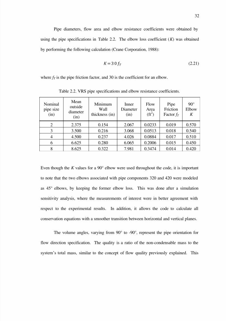
32
Pipe diameters, flow area and elbow resistance coefficients were obtained by
using the pipe specifications in Table 2.2. The elbow loss coefficient (K ) was obtained
by performing the following calculation (Crane Corporation, 1988):
(2.21)
where f T is the pipe friction factor, and 30 is the coefficient for an elbow.
Table 2.2. VRS pipe specifications and elbow resistance coefficients.
Nominalpipe size
(in)
Mean
outside
diameter(in)
MinimumWall
thickness (in)
InnerDiameter
(in)
FlowArea
(ft2)
PipeFriction
Factor f T
90°Elbow
K
2 2.375 0.154 2.067 0.0233 0.019 0.570
3 3.500 0.216 3.068 0.0513 0.018 0.540
4 4.500 0.237 4.026 0.0884 0.017 0.510
6 6.625 0.280 6.065 0.2006 0.015 0.450
8 8.625 0.322 7.981 0.3474 0.014 0.420
Even though the K values for a 90° elbow were used throughout the code, it is important
to note that the two elbows associated with pipe components 320 and 420 were modeled
as 45° elbows, by keeping the former elbow loss. This was done after a simulation
sensitivity analysis, where the measurements of interest were in better agreement with
respect to the experimental results. In addition, it allows the code to calculate all
conservation equations with a smoother transition between horizontal and vertical planes.
The volume angles, varying from 90° to -90°, represent the pipe orientation for
flow direction specification. The quality is a ratio of the non-condensable mass to the
system‘s total mass, similar to the concept of flow quality previously explained. This

7/29/2019 Simulation and Validation of Two-component Flow in a Void Recircu
http://slidepdf.com/reader/full/simulation-and-validation-of-two-component-flow-in-a-void-recircu 49/171
33
value was defined as zero throughout all piping networks since there was no initial air in
the system. Instead, air was injected into the pipes at steady-state conditions.
The volume centroid elevation and pressure were calculated using the following
expressions:
(2.22)
(2.23)
where elevation of the ith volume centroid (ft)
length of the ith volume (ft)
angle of the ith volume measured from horizontal (degrees)
diameter of the ith volume (in)
pressure of the ith volume (psi)
phasic specific volume of the ith volume (ft3 /lb)
The volume centroid elevation and pressure will remain the same if the volume angle is
zero.
Enlargements and contractions (reducing bushings) were modeled by inputting
the forward and reverse loss coefficients into the PIPE model. Forward and reverse loss
coefficients are used for co-current and counter-current flows, respectively. The loss

7/29/2019 Simulation and Validation of Two-component Flow in a Void Recircu
http://slidepdf.com/reader/full/simulation-and-validation-of-two-component-flow-in-a-void-recircu 50/171
34
coefficient (K ) for enlargements and contractions, were calculated by using the following
expressions (Crane Corporation, 1988):
(2.24)
(2.25)
where is the ratio of diameters of the small ( D1) to large ( D2) pipes, and is the angle
of divergence measured in radians. The divergence angle must satisfy the condition
45°< 180° and was calculated as:
(2.26)
Where N is the socket to socket bottom dimension (Spears Manufacturing Company,
2010). Table 2.3 summarizes all loss coefficient values for several enlargement and
contraction devices used in the VRS model.
Table 2.3. Enlargement and contraction loss coefficient values for various reducing
bushings.
Largediameter
D2 (in)
Smalldiameter
D1 (in)
Reducing
Bushing
Dimension
N (in)ω (rad)
Enlargement
K
Contraction
K
3 2 3x2 0.563 1.058 0.309 0.999
4 2 4x2 1.031 1.095 0.563 4.328
4 3 4x3 0.469 1.132 0.191 0.506
6 2 6x2 2.156 1.076 0.790 25.774
6 3 6x3 1.625 1.074 0.563 4.292
6 4 6x4 1.563 0.908 0.309 0.931
7/29/2019 Simulation and Validation of Two-component Flow in a Void Recircu
http://slidepdf.com/reader/full/simulation-and-validation-of-two-component-flow-in-a-void-recircu 51/171
7/29/2019 Simulation and Validation of Two-component Flow in a Void Recircu
http://slidepdf.com/reader/full/simulation-and-validation-of-two-component-flow-in-a-void-recircu 52/171
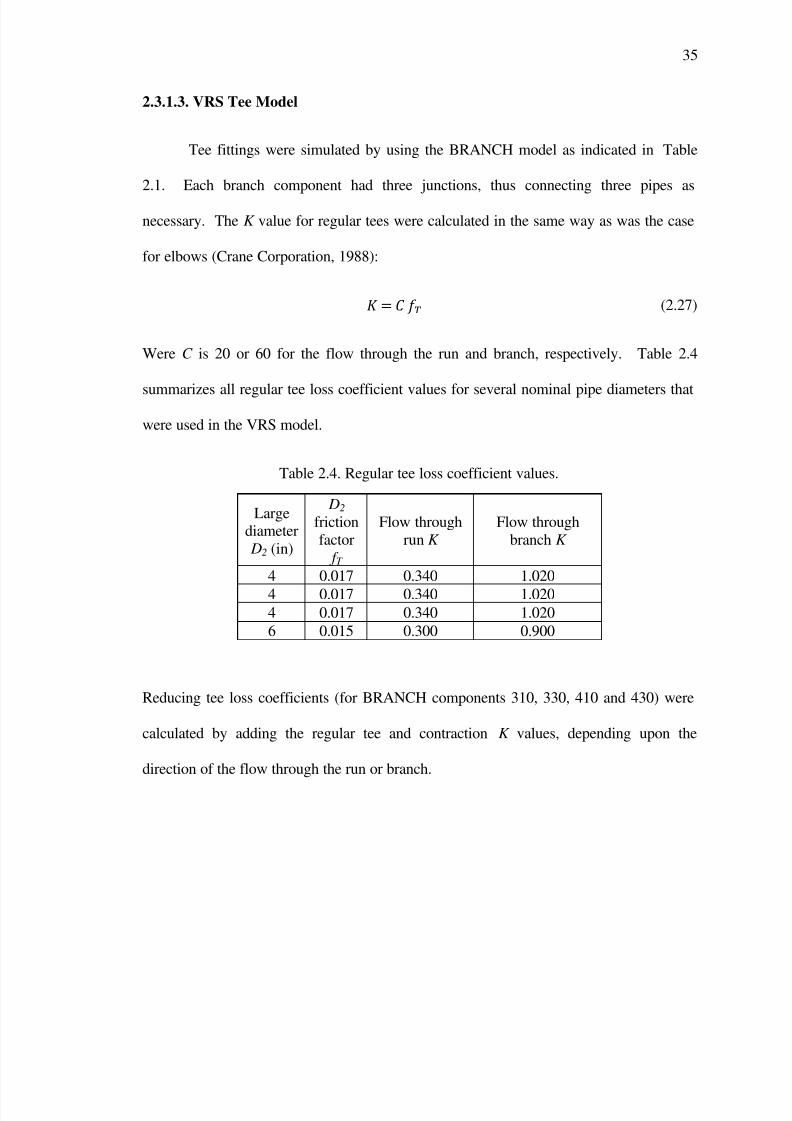
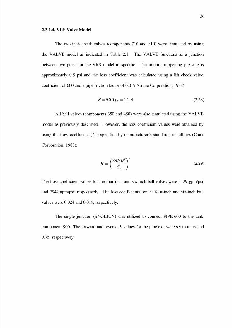
36
2.3.1.4. VRS Valve Model
The two-inch check valves (components 710 and 810) were simulated by using
the VALVE model as indicated in Table 2.1. The VALVE functions as a junction
between two pipes for the VRS model in specific. The minimum opening pressure is
approximately 0.5 psi and the loss coefficient was calculated using a lift check valve
coefficient of 600 and a pipe friction factor of 0.019 (Crane Corporation, 1988):
(2.28)
All ball valves (components 350 and 450) were also simulated using the VALVE
model as previously described. However, the loss coefficient values were obtained by
using the flow coefficient (C V ) specified by manufacturer‘s standards as follows (Crane
Corporation, 1988):
(2.29)
The flow coefficient values for the four-inch and six-inch ball valves were 3129 gpm/psi
and 7942 gpm/psi, respectively. The loss coefficients for the four-inch and six-inch ball
valves were 0.024 and 0.019, respectively.
The single junction (SNGLJUN) was utilized to connect PIPE-600 to the tank
component 900. The forward and reverse K values for the pipe exit were set to unity and
0.75, respectively.
7/29/2019 Simulation and Validation of Two-component Flow in a Void Recircu
http://slidepdf.com/reader/full/simulation-and-validation-of-two-component-flow-in-a-void-recircu 53/171
37
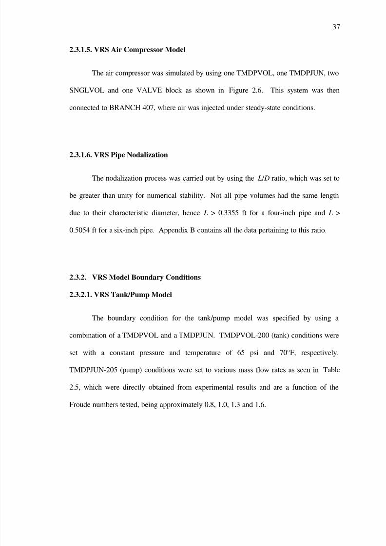
2.3.1.5. VRS Air Compressor Model
The air compressor was simulated by using one TMDPVOL, one TMDPJUN, two
SNGLVOL and one VALVE block as shown in Figure 2.6. This system was then
connected to BRANCH 407, where air was injected under steady-state conditions.
2.3.1.6. VRS Pipe Nodalization
The nodalization process was carried out by using the L / D ratio, which was set to
be greater than unity for numerical stability. Not all pipe volumes had the same length
due to their characteristic diameter, hence L > 0.3355 ft for a four-inch pipe and L >
0.5054 ft for a six-inch pipe. Appendix B contains all the data pertaining to this ratio.
2.3.2. VRS Model Boundary Conditions
2.3.2.1. VRS Tank/Pump Model
The boundary condition for the tank/pump model was specified by using a
combination of a TMDPVOL and a TMDPJUN. TMDPVOL-200 (tank) conditions were
set with a constant pressure and temperature of 65 psi and 70°F, respectively.
TMDPJUN-205 (pump) conditions were set to various mass flow rates as seen in Table
2.5, which were directly obtained from experimental results and are a function of the
Froude numbers tested, being approximately 0.8, 1.0, 1.3 and 1.6.
7/29/2019 Simulation and Validation of Two-component Flow in a Void Recircu
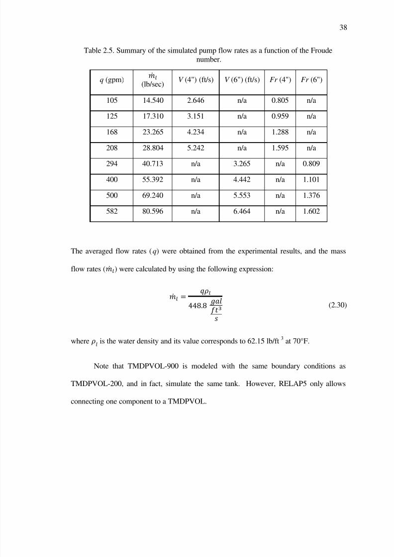
http://slidepdf.com/reader/full/simulation-and-validation-of-two-component-flow-in-a-void-recircu 54/171
38
Table 2.5. Summary of the simulated pump flow rates as a function of the Froude
number.
q (gpm)
(lb/sec)V (4") (ft/s) V (6") (ft/s) Fr (4") Fr (6")
105 14.540 2.646 n/a 0.805 n/a
125 17.310 3.151 n/a 0.959 n/a
168 23.265 4.234 n/a 1.288 n/a
208 28.804 5.242 n/a 1.595 n/a
294 40.713 n/a 3.265 n/a 0.809
400 55.392 n/a 4.442 n/a 1.101
500 69.240 n/a 5.553 n/a 1.376
582 80.596 n/a 6.464 n/a 1.602
The averaged flow rates (q) were obtained from the experimental results, and the mass
flow rates ( ) were calculated by using the following expression:
(2.30)
where is the water density and its value corresponds to 62.15 lb/ft3
at 70°F.
Note that TMDPVOL-900 is modeled with the same boundary conditions as
TMDPVOL-200, and in fact, simulate the same tank. However, RELAP5 only allows
connecting one component to a TMDPVOL.
7/29/2019 Simulation and Validation of Two-component Flow in a Void Recircu
http://slidepdf.com/reader/full/simulation-and-validation-of-two-component-flow-in-a-void-recircu 55/171

7/29/2019 Simulation and Validation of Two-component Flow in a Void Recircu
http://slidepdf.com/reader/full/simulation-and-validation-of-two-component-flow-in-a-void-recircu 56/171
40
Table 2.6. Air injection scheme for various Froude numbers in the four-inch pipe,
yielding a minimum initial void fraction of seven-percent.
Air Flow Rate (lb/s) - 4" pipe
Injection Time (s) Fr = 0.81 Fr = 0.96 Fr = 1.29 Fr = 1.600-15 0 0 0 0
16 0 0 5.00E-04 1.00E-03
17 0 5.00E-04 1.00E-03 2.00E-03
18 5.00E-04 1.00E-03 2.00E-03 3.00E-03
19 1.00E-03 2.50E-03 3.00E-03 4.00E-03
20-35 3.00E-03 3.30E-03 3.80E-03 4.50E-03
36 2.80E-03 3.00E-03 3.50E-03 4.00E-03
37 2.60E-03 2.00E-03 3.00E-03 3.00E-03
38 2.40E-03 1.00E-03 2.00E-03 2.00E-03
39 2.00E-03 5.00E-04 1.00E-03 1.00E-03
40 1.60E-03 0 5.00E-04 5.00E-04
41 1.20E-03 0 0 0
42 0 0 0 0
Table 2.7. Air injection scheme for various Froude numbers in the six-inch pipe, yielding
a minimum initial void fraction of seven-percent.
Air Flow Rate (lb/s) - 6" pipe
Injection Time (s) Fr = 0.81 Fr = 1.10 Fr = 1.38 Fr = 1.60
0-15 0 0 0 0
16 0 0 0 1.00E-03
17 1.00E-03 1.00E-03 1.00E-03 5.00E-03
18 3.00E-03 3.00E-03 5.00E-03 7.00E-03
19 5.00E-03 5.00E-03 7.00E-03 1.20E-02
20-35 7.80E-03 9.70E-03 1.20E-02 1.48E-02
36 5.00E-03 6.00E-03 6.00E-03 6.00E-03
37 3.00E-03 3.00E-03 3.00E-03 3.00E-03
38 1.00E-03 1.00E-03 1.00E-03 1.00E-03
39 0 0 0 040 0 0 0 0

7/29/2019 Simulation and Validation of Two-component Flow in a Void Recircu
http://slidepdf.com/reader/full/simulation-and-validation-of-two-component-flow-in-a-void-recircu 57/171
41
2.3.3. VRS Model Thermal/Hydraulic settings
RELAP5 uses two different set of control flags that allow the calculation of
specific thermal/hydraulic models (RELAP5/MOD3.2, Code Manual Volume II: User's
Guide and Input Requirements, 1995). It is up to the user to use them accordingly
depending upon the simulation being carried. The first set of control flags consist of the
packed format tlpvbfe, which allows the processing of the following models:
t – Thermal front tracking model: used to improve the accuracy calculations when
a warm fluid layer appears above a cold fluid.
l – Mixture level tracking model: used to calculate the void fractions (above and
below level) and level velocity in a volume.
p – Water packing scheme: used to model a pressurizer.
v – Vertical stratification model: used to model a pressurizer.
b – Interphase friction model: used to model the pipe or rod bundle interphase
friction.
f – Wall friction model: used to specify if the wall friction effects are to be
accounted for.
e – Non-equilibrium model, used to specify the non-equilibrium or equilibrium
model. This option is provided for the comparison between other codes.
The second set of control flags consist of the packed format efvcahs, which allows the
processing of the following models:
7/29/2019 Simulation and Validation of Two-component Flow in a Void Recircu
http://slidepdf.com/reader/full/simulation-and-validation-of-two-component-flow-in-a-void-recircu 58/171
42
e – modified PV (pressure-volume) term: used to specify if the PV term is to be
applied.
f – Counter-current Flow Limitation (CCFL) model: used specifically for vertical
volumes, gas-liquid phases and counter-current flow (liquid flowing down,
gas flowing up).
v – Horizontal stratification model, used to model a BRANCH component.
c – Choking model: recommended to be used for modeling relief valves.
Removal of the choking model may be recommended to avoid internal
oscillations.
a – Abrupt area model: used when sharp edged area changes occur; recommended
to be used in a BRANCH component.
h – Non-homogenous model: used to specify the non-homogeneous (two-velocity
momentum equations) or homogenous (single-velocity momentum equation)
options.
s – Momentum flux model: used in BRANCH components; specifies the use of
the momentum flux in the BRANCH junctions.
Table 2.8 shows the summary of the control flags used in the main VRS model
components, including the tank/pump, pipe, regular tees, check valves and ball valves.
The letter ‗X‘ is used to symbolize that the current model is being used. The letters ‗N-
E‘, ‗N-H‘, ‗S‘, and ‗A‘ stand for non-equilibrium, non-homogenous, smooth area change,
and abrupt area change, respectively.
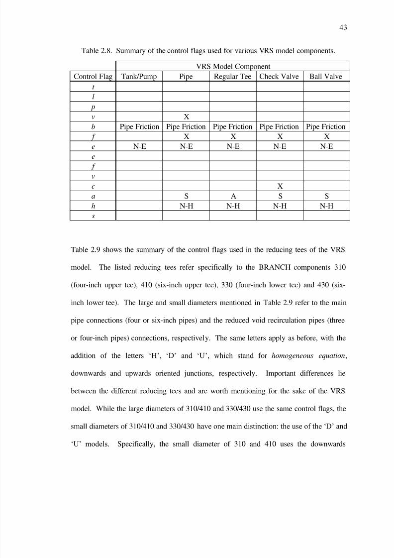
7/29/2019 Simulation and Validation of Two-component Flow in a Void Recircu
http://slidepdf.com/reader/full/simulation-and-validation-of-two-component-flow-in-a-void-recircu 59/171
43
Table 2.8. Summary of the control flags used for various VRS model components.
VRS Model Component
Control Flag Tank/Pump Pipe Regular Tee Check Valve Ball Valve
t
l p
v X
b Pipe Friction Pipe Friction Pipe Friction Pipe Friction Pipe Friction
f X X X X
e N-E N-E N-E N-E N-E
e
f
v
c X
a S A S Sh N-H N-H N-H N-H
s
Table 2.9 shows the summary of the control flags used in the reducing tees of the VRS
model. The listed reducing tees refer specifically to the BRANCH components 310
(four-inch upper tee), 410 (six-inch upper tee), 330 (four-inch lower tee) and 430 (six-
inch lower tee). The large and small diameters mentioned in Table 2.9 refer to the main
pipe connections (four or six-inch pipes) and the reduced void recirculation pipes (three
or four-inch pipes) connections, respectively. The same letters apply as before, with the
addition of the letters ‗H‘, ‗D‘ and ‗U‘, which stand for homogeneous equation,
downwards and upwards oriented junctions, respectively. Important differences lie
between the different reducing tees and are worth mentioning for the sake of the VRS
model. While the large diameters of 310/410 and 330/430 use the same control flags, the
small diameters of 310/410 and 330/430 have one main distinction: the use of the ‗D‘ and
‗U‘ models. Specifically, the small diameter of 310 and 410 uses the downwards
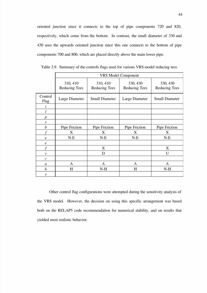
7/29/2019 Simulation and Validation of Two-component Flow in a Void Recircu
http://slidepdf.com/reader/full/simulation-and-validation-of-two-component-flow-in-a-void-recircu 60/171
7/29/2019 Simulation and Validation of Two-component Flow in a Void Recircu
http://slidepdf.com/reader/full/simulation-and-validation-of-two-component-flow-in-a-void-recircu 61/171
45
2.3.3.1. VRS Valve Model
The valve model only uses the packed format efvcahs, where the choking model
(c) is only used for the check valve, recommendation done by RELAP5 for relief valves.
All other process models were not used on both check and ball valves.
2.4. Fluid Properties
The fluids used in the VRS model are water for the liquid phase and air (non-
condensable) for the gas phase. Both fluids were set at a temperature of 70°F, and at
different pressures depending on the component used. RELAP5 automatically calculates
all fluid properties once the types of fluids, temperatures and pressures have been
specified.
2.5. Simulation Assumptions
The VRS model, built in RELAP5, was created under the following assumptions:
All simulations happen on the discharge side of the pump, rather than on
the suction side. These simulations are intended to be benchmarked with
the experimental results, which were also carried on the discharge side of
the pump.
Air injection occurs when the main flow is steady-state, assuming the
pump has been running for a certain amount of time.

7/29/2019 Simulation and Validation of Two-component Flow in a Void Recircu
http://slidepdf.com/reader/full/simulation-and-validation-of-two-component-flow-in-a-void-recircu 62/171
46
The Froude number parameters, which are meant to describe the water
velocities, are assumed to be referenced to the main four and six-inch
pipes, with water occupying the entire cross-section of the pipe.
The VRS tank is modeled as a water reservoir, having a constant pressure.
The VRS pump is modeled with a constant supply of water, rather than
using a pump curve, for better code handling.
The kinematic shock phenomenon is replaced by adding a slightly greater
amount of air than that recorded during the experiment.
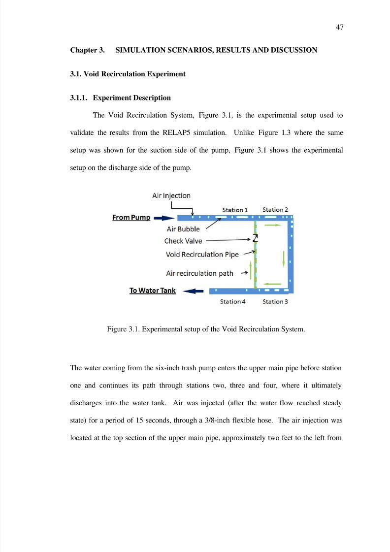
7/29/2019 Simulation and Validation of Two-component Flow in a Void Recircu
http://slidepdf.com/reader/full/simulation-and-validation-of-two-component-flow-in-a-void-recircu 63/171
47
Chapter 3. SIMULATION SCENARIOS, RESULTS AND DISCUSSION
3.1. Void Recirculation Experiment
3.1.1. Experiment Description
The Void Recirculation System, Figure 3.1, is the experimental setup used to
validate the results from the RELAP5 simulation. Unlike Figure 1.3 where the same
setup was shown for the suction side of the pump, Figure 3.1 shows the experimental
setup on the discharge side of the pump.
Figure 3.1. Experimental setup of the Void Recirculation System.
The water coming from the six-inch trash pump enters the upper main pipe before station
one and continues its path through stations two, three and four, where it ultimately
discharges into the water tank. Air was injected (after the water flow reached steady
state) for a period of 15 seconds, through a 3/8-inch flexible hose. The air injection was
located at the top section of the upper main pipe, approximately two feet to the left from
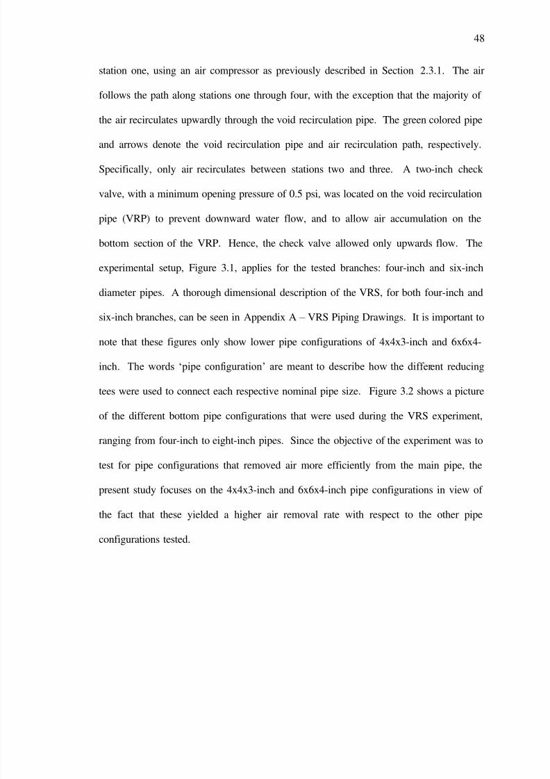
7/29/2019 Simulation and Validation of Two-component Flow in a Void Recircu
http://slidepdf.com/reader/full/simulation-and-validation-of-two-component-flow-in-a-void-recircu 64/171
48
station one, using an air compressor as previously described in Section 2.3.1. The air
follows the path along stations one through four, with the exception that the majority of
the air recirculates upwardly through the void recirculation pipe. The green colored pipe
and arrows denote the void recirculation pipe and air recirculation path, respectively.
Specifically, only air recirculates between stations two and three. A two-inch check
valve, with a minimum opening pressure of 0.5 psi, was located on the void recirculation
pipe (VRP) to prevent downward water flow, and to allow air accumulation on the
bottom section of the VRP. Hence, the check valve allowed only upwards flow. The
experimental setup, Figure 3.1, applies for the tested branches: four-inch and six-inch
diameter pipes. A thorough dimensional description of the VRS, for both four-inch and
six-inch branches, can be seen in Appendix A – VRS Piping Drawings. It is important to
note that these figures only show lower pipe configurations of 4x4x3-inch and 6x6x4-
inch. The words ‗pipe configuration‘ are meant to describe how the differ ent reducing
tees were used to connect each respective nominal pipe size. Figure 3.2 shows a picture
of the different bottom pipe configurations that were used during the VRS experiment,
ranging from four-inch to eight-inch pipes. Since the objective of the experiment was to
test for pipe configurations that removed air more efficiently from the main pipe, the
present study focuses on the 4x4x3-inch and 6x6x4-inch pipe configurations in view of
the fact that these yielded a higher air removal rate with respect to the other pipe
configurations tested.
7/29/2019 Simulation and Validation of Two-component Flow in a Void Recircu
http://slidepdf.com/reader/full/simulation-and-validation-of-two-component-flow-in-a-void-recircu 65/171
49
Figure 3.2. Lower pipe configurations used during the VRS experiment.
The main parameters controlled during the VRS experiment were initial void
fraction and main pipe flow rate. Void fraction measurements were determined visually
using square level rulers with 1/8-inch measurement resolution, located at stations one
through four, where station one was used to determine the initial void fraction. The
initial void fractions during the VRS experiment varied between three and 13 percent for
the different pipe configurations tested. The initial void fraction to be analyzed under the
present study is approximately seven percent for both pipe configurations 4x4x3-inch and
6x6x4-inch. The void fraction value of seven percent was carefully chosen since it
appears in both pipe configuration results, allowing easy comparison. The maximum
allowable void fraction in station four of the VRS model and test fixture is five percent

7/29/2019 Simulation and Validation of Two-component Flow in a Void Recircu
http://slidepdf.com/reader/full/simulation-and-validation-of-two-component-flow-in-a-void-recircu 66/171
50
for pipe diameters less than 12 inches. This five percent void fraction value is based on
nuclear industry acceptability and on-going research (Institute of Nuclear Power
Operations, 2010). Flow rate measurements were determined electronically using a
turbine paddle flow meter, located on the main six-inch pipe after the pump as depicted in
Figure 2.6. Flow rate values were then converted to Froude numbers to allow easy
comparison between the different pipe diameters tested. A summary of the different flow
rates tested for both pipe branches can be seen in Table 2.5 for further reference. Three
different trials were measured with the same initial void fraction and Froude number.
The void fraction recorded at each station was a visual average for the period of time of
each trial (approximately two minutes or 120 seconds). Hence, only three void fraction
values taken from each trial were reported for each scenario. Even though the
experimental results were insufficient for a thorough statistical analysis, it provides an
insight of the values to be expected at each station and will be used to validate the
numerical results obtained from RELAP5.
The experiment setup was chosen to be in this specific way for two main reasons:
first, to have better flow rate control and second, to avoid the rather complicated vacuum
running conditions. Even though air behaves differently under suction and discharge
conditions, the recirculation behavior was the main objective to prove that the VRS
device worked properly.
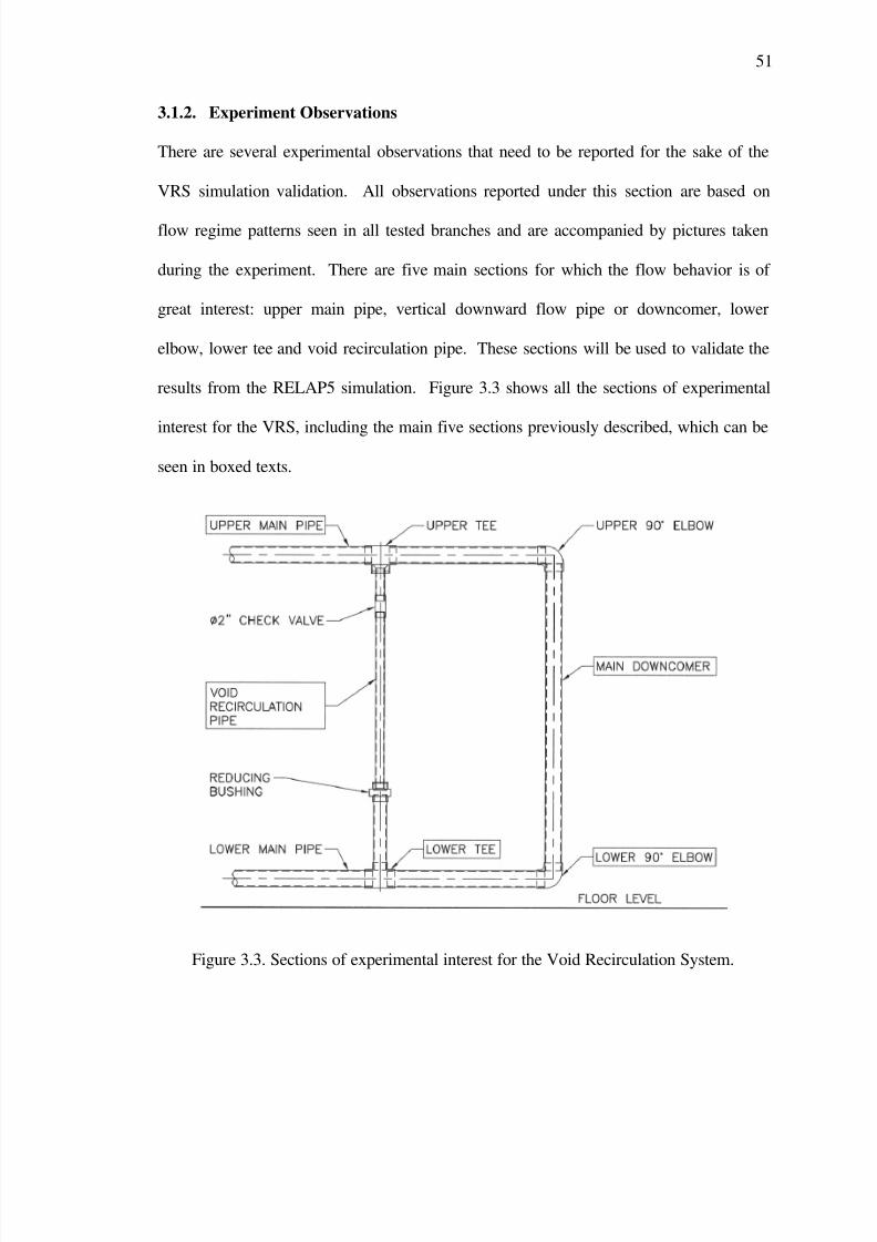
7/29/2019 Simulation and Validation of Two-component Flow in a Void Recircu
http://slidepdf.com/reader/full/simulation-and-validation-of-two-component-flow-in-a-void-recircu 67/171
51
3.1.2. Experiment Observations
There are several experimental observations that need to be reported for the sake of the
VRS simulation validation. All observations reported under this section are based on
flow regime patterns seen in all tested branches and are accompanied by pictures taken
during the experiment. There are five main sections for which the flow behavior is of
great interest: upper main pipe, vertical downward flow pipe or downcomer, lower
elbow, lower tee and void recirculation pipe. These sections will be used to validate the
results from the RELAP5 simulation. Figure 3.3 shows all the sections of experimental
interest for the VRS, including the main five sections previously described, which can be
seen in boxed texts.
Figure 3.3. Sections of experimental interest for the Void Recirculation System.
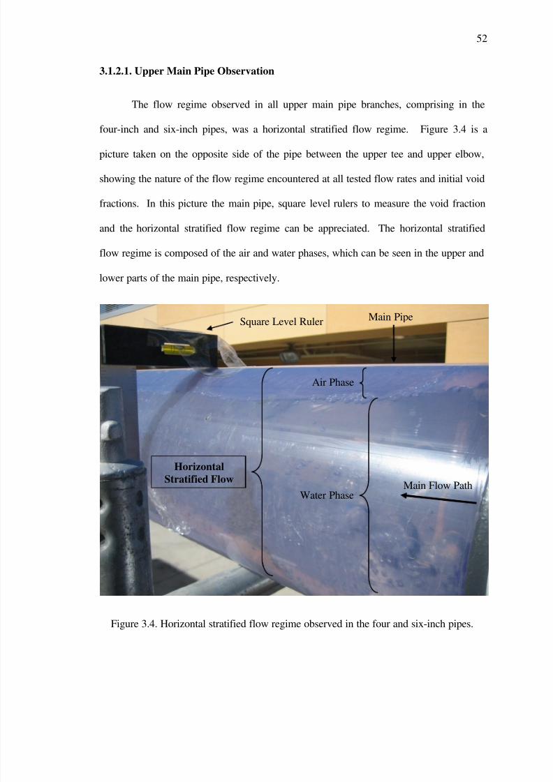
7/29/2019 Simulation and Validation of Two-component Flow in a Void Recircu
http://slidepdf.com/reader/full/simulation-and-validation-of-two-component-flow-in-a-void-recircu 68/171
52
3.1.2.1. Upper Main Pipe Observation
The flow regime observed in all upper main pipe branches, comprising in the
four-inch and six-inch pipes, was a horizontal stratified flow regime. Figure 3.4 is a
picture taken on the opposite side of the pipe between the upper tee and upper elbow,
showing the nature of the flow regime encountered at all tested flow rates and initial void
fractions. In this picture the main pipe, square level rulers to measure the void fraction
and the horizontal stratified flow regime can be appreciated. The horizontal stratified
flow regime is composed of the air and water phases, which can be seen in the upper and
lower parts of the main pipe, respectively.
Figure 3.4. Horizontal stratified flow regime observed in the four and six-inch pipes.
Square Level Ruler
Horizontal
Stratified Flow
Air Phase
Water Phase
Main Pipe
Main Flow Path
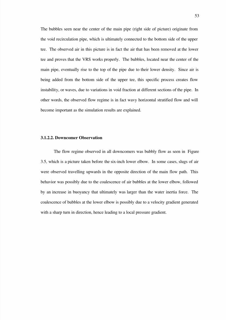
7/29/2019 Simulation and Validation of Two-component Flow in a Void Recircu
http://slidepdf.com/reader/full/simulation-and-validation-of-two-component-flow-in-a-void-recircu 69/171
53
The bubbles seen near the center of the main pipe (right side of picture) originate from
the void recirculation pipe, which is ultimately connected to the bottom side of the upper
tee. The observed air in this picture is in fact the air that has been removed at the lower
tee and proves that the VRS works properly. The bubbles, located near the center of the
main pipe, eventually rise to the top of the pipe due to their lower density. Since air is
being added from the bottom side of the upper tee, this specific process creates flow
instability, or waves, due to variations in void fraction at different sections of the pipe. In
other words, the observed flow regime is in fact wavy horizontal stratified flow and will
become important as the simulation results are explained.
3.1.2.2. Downcomer Observation
The flow regime observed in all downcomers was bubbly flow as seen in Figure
3.5, which is a picture taken before the six-inch lower elbow. In some cases, slugs of air
were observed travelling upwards in the opposite direction of the main flow path. This
behavior was possibly due to the coalescence of air bubbles at the lower elbow, followed
by an increase in buoyancy that ultimately was larger than the water inertia force. The
coalescence of bubbles at the lower elbow is possibly due to a velocity gradient generated
with a sharp turn in direction, hence leading to a local pressure gradient.
7/29/2019 Simulation and Validation of Two-component Flow in a Void Recircu
http://slidepdf.com/reader/full/simulation-and-validation-of-two-component-flow-in-a-void-recircu 70/171
54
Figure 3.5. Downward bubbly flow regime observed in the four and six-inch pipes.
3.1.2.3. Lower Elbow Observation
The flow regimes observed after the lower elbow for all tested pipe branches
varied between wavy horizontally stratified, slug and bubbly flow. Figure 3.6 shows the
wavy horizontal stratified flow observed at one instant of time, with bubbly flow in the
water phase. These bubbles, due to their lower density, eventually rise and help generate
waves downstream. Figure 3.7 shows a combination between bubbly and slug flow in a
short length of pipe and at a later instant of time than Figure 3.6. The bubbly flow is
shown to the left, immediately after the lower elbow and the slug flow is shown to the
Main Pipe
Air bubbles
Bottom Elbow
Main Flow Path
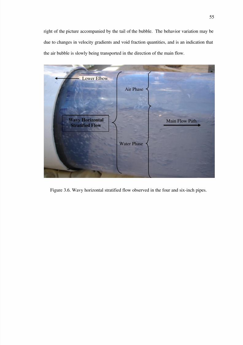
7/29/2019 Simulation and Validation of Two-component Flow in a Void Recircu
http://slidepdf.com/reader/full/simulation-and-validation-of-two-component-flow-in-a-void-recircu 71/171
55
right of the picture accompanied by the tail of the bubble. The behavior variation may be
due to changes in velocity gradients and void fraction quantities, and is an indication that
the air bubble is slowly being transported in the direction of the main flow.
Figure 3.6. Wavy horizontal stratified flow observed in the four and six-inch pipes.
Wavy HorizontalStratified Flow
Air Phase
Water Phase
Main Flow Path
Lower Elbow

7/29/2019 Simulation and Validation of Two-component Flow in a Void Recircu
http://slidepdf.com/reader/full/simulation-and-validation-of-two-component-flow-in-a-void-recircu 72/171
56
Figure 3.7 Bubbly and slug flow observed in the four and six-inch pipes.
Finally, it was observed that in many cases an air bubble would form,
immediately after the lower elbow, with a defined bubble head. This bubble would move
back and forth for a period of time, with a severe change in void fraction but no net
velocity, until water broke the air bubble by allowing it to move in the direction of the
main flow. When the breaking process happened, the air bubble accelerated until it
reached the velocity of the water. This phenomenon can be clearly depicted in the
following section and will become important for simulation validation.
Main Flow Path
Slug Flow
Bubbly Flow
Lower Elbow
Bubble Tail
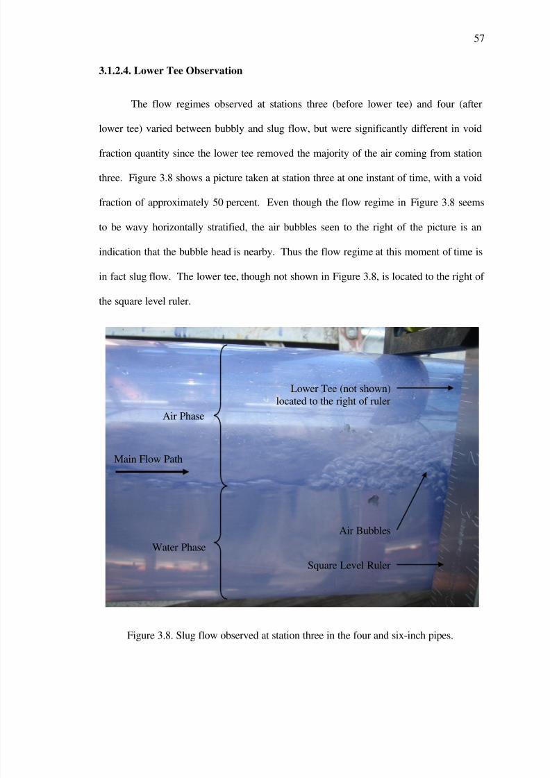
7/29/2019 Simulation and Validation of Two-component Flow in a Void Recircu
http://slidepdf.com/reader/full/simulation-and-validation-of-two-component-flow-in-a-void-recircu 73/171
57
3.1.2.4. Lower Tee Observation
The flow regimes observed at stations three (before lower tee) and four (after
lower tee) varied between bubbly and slug flow, but were significantly different in void
fraction quantity since the lower tee removed the majority of the air coming from station
three. Figure 3.8 shows a picture taken at station three at one instant of time, with a void
fraction of approximately 50 percent. Even though the flow regime in Figure 3.8 seems
to be wavy horizontally stratified, the air bubbles seen to the right of the picture is an
indication that the bubble head is nearby. Thus the flow regime at this moment of time is
in fact slug flow. The lower tee, though not shown in Figure 3.8, is located to the right of
the square level ruler.
Figure 3.8. Slug flow observed at station three in the four and six-inch pipes.
Air Phase
Water Phase
Main Flow Path
Square Level Ruler
Air Bubbles
Lower Tee (not shown)
located to the right of ruler
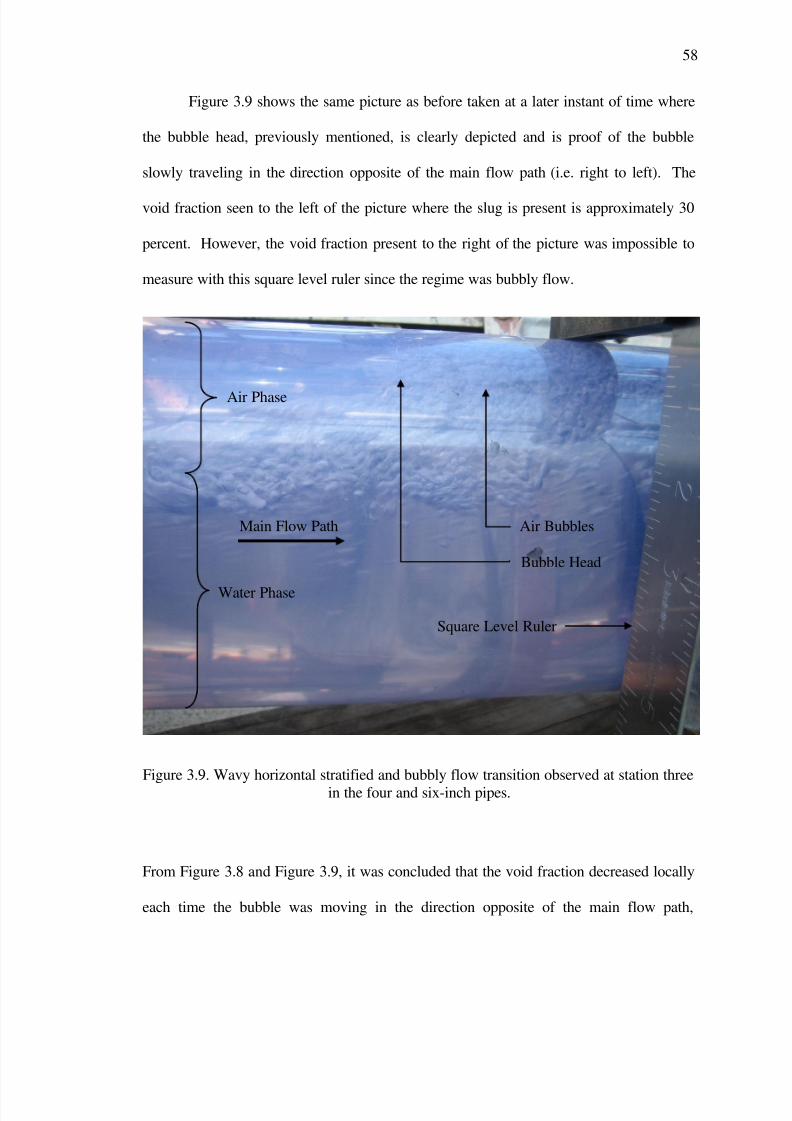
7/29/2019 Simulation and Validation of Two-component Flow in a Void Recircu
http://slidepdf.com/reader/full/simulation-and-validation-of-two-component-flow-in-a-void-recircu 74/171
58
Figure 3.9 shows the same picture as before taken at a later instant of time where
the bubble head, previously mentioned, is clearly depicted and is proof of the bubble
slowly traveling in the direction opposite of the main flow path (i.e. right to left). The
void fraction seen to the left of the picture where the slug is present is approximately 30
percent. However, the void fraction present to the right of the picture was impossible to
measure with this square level ruler since the regime was bubbly flow.
Figure 3.9. Wavy horizontal stratified and bubbly flow transition observed at station three
in the four and six-inch pipes.
From Figure 3.8 and Figure 3.9, it was concluded that the void fraction decreased locally
each time the bubble was moving in the direction opposite of the main flow path,
Square Level Ruler
Air Bubbles
Bubble Head
Air Phase
Water Phase
Main Flow Path
7/29/2019 Simulation and Validation of Two-component Flow in a Void Recircu
http://slidepdf.com/reader/full/simulation-and-validation-of-two-component-flow-in-a-void-recircu 75/171
59
implying that the air velocity would range between zero and negative values. In contrast,
the void fraction increased locally whenever the bubble traveled in the direction of the
main flow path, implying that the air velocity would range between zero and positive
values. This behavior supports the discussion provided in the previous section (3.1.2.3),
where the bubble moves back and forth for a period of time, until there is enough void
fraction with respect to the main flow to disrupt the air bubble, allowing it to travel in the
direction of the main flow path.
The flow regime observed at station four was mainly bubbly with little amount of
void fraction as seen in Figure 3.10. Occasionally, slugs of air were observed with
approximately 20 percent void fraction, but only for a short period of time. This behavior
may be due to a flow discontinuity generated by the lower tee, which will be further
discussed in the next section.
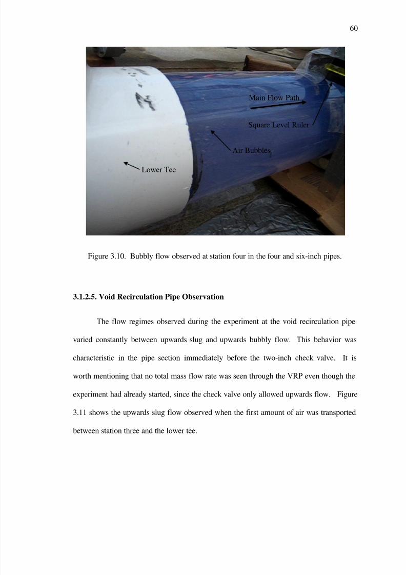
7/29/2019 Simulation and Validation of Two-component Flow in a Void Recircu
http://slidepdf.com/reader/full/simulation-and-validation-of-two-component-flow-in-a-void-recircu 76/171
60
Figure 3.10. Bubbly flow observed at station four in the four and six-inch pipes.
3.1.2.5. Void Recirculation Pipe Observation
The flow regimes observed during the experiment at the void recirculation pipe
varied constantly between upwards slug and upwards bubbly flow. This behavior was
characteristic in the pipe section immediately before the two-inch check valve. It is
worth mentioning that no total mass flow rate was seen through the VRP even though the
experiment had already started, since the check valve only allowed upwards flow. Figure
3.11 shows the upwards slug flow observed when the first amount of air was transported
between station three and the lower tee.
Lower Tee
Air Bubbles
Main Flow Path
Square Level Ruler

7/29/2019 Simulation and Validation of Two-component Flow in a Void Recircu
http://slidepdf.com/reader/full/simulation-and-validation-of-two-component-flow-in-a-void-recircu 77/171
61
Figure 3.11. Upwards slug flow observed at the VRP for the four and six-inch pipe
configurations.
The head of the bubble, which takes the form of a bullet shape, matches the description of
the Taylor bubbles seen in Figure 2.3, and can be seen towards the top of the picture.
The bubble head is followed by the bubble body seen in the middle of the picture, which
is occupying nearly 90 percent of the inner pipe diameter. This slug of air forces the
water to move sideways towards the wall (thin water wall formation) and downwards,
until no more slugs are present, for which at this time bubbly flow occurs as shown in
Figure 3.12. The flow regime in this section of pipe varied between slug and bubbly
Main Flow Path
Bubble Head
Water Phase
Air Phase
Thin Water Wall
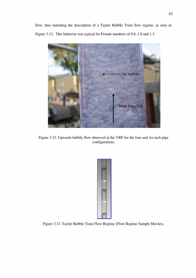
7/29/2019 Simulation and Validation of Two-component Flow in a Void Recircu
http://slidepdf.com/reader/full/simulation-and-validation-of-two-component-flow-in-a-void-recircu 78/171
62
flow, thus matching the description of a Taylor Bubble Train flow regime, as seen in
Figure 3.13. This behavior was typical for Froude numbers of 0.8, 1.0 and 1.3.
Figure 3.12. Upwards bubbly flow observed at the VRP for the four and six-inch pipe
configurations.
Figure 3.13. Taylor Bubble Train Flow Regime (Flow Regime Sample Movies).
Main Flow Path
Air bubbles
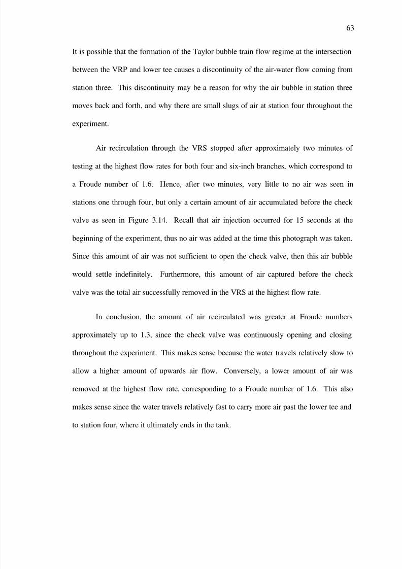
7/29/2019 Simulation and Validation of Two-component Flow in a Void Recircu
http://slidepdf.com/reader/full/simulation-and-validation-of-two-component-flow-in-a-void-recircu 79/171
63
It is possible that the formation of the Taylor bubble train flow regime at the intersection
between the VRP and lower tee causes a discontinuity of the air-water flow coming from
station three. This discontinuity may be a reason for why the air bubble in station three
moves back and forth, and why there are small slugs of air at station four throughout the
experiment.
Air recirculation through the VRS stopped after approximately two minutes of
testing at the highest flow rates for both four and six-inch branches, which correspond to
a Froude number of 1.6. Hence, after two minutes, very little to no air was seen in
stations one through four, but only a certain amount of air accumulated before the check
valve as seen in Figure 3.14. Recall that air injection occurred for 15 seconds at the
beginning of the experiment, thus no air was added at the time this photograph was taken.
Since this amount of air was not sufficient to open the check valve, then this air bubble
would settle indefinitely. Furthermore, this amount of air captured before the check
valve was the total air successfully removed in the VRS at the highest flow rate.
In conclusion, the amount of air recirculated was greater at Froude numbers
approximately up to 1.3, since the check valve was continuously opening and closing
throughout the experiment. This makes sense because the water travels relatively slow to
allow a higher amount of upwards air flow. Conversely, a lower amount of air was
removed at the highest flow rate, corresponding to a Froude number of 1.6. This also
makes sense since the water travels relatively fast to carry more air past the lower tee and
to station four, where it ultimately ends in the tank.
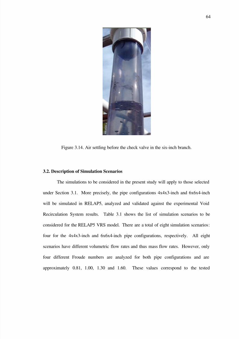
7/29/2019 Simulation and Validation of Two-component Flow in a Void Recircu
http://slidepdf.com/reader/full/simulation-and-validation-of-two-component-flow-in-a-void-recircu 80/171
64
Figure 3.14. Air settling before the check valve in the six-inch branch.
3.2. Description of Simulation Scenarios
The simulations to be considered in the present study will apply to those selected
under Section 3.1. More precisely, the pipe configurations 4x4x3-inch and 6x6x4-inch
will be simulated in RELAP5, analyzed and validated against the experimental Void
Recirculation System results. Table 3.1 shows the list of simulation scenarios to be
considered for the RELAP5 VRS model. There are a total of eight simulation scenarios:
four for the 4x4x3-inch and 6x6x4-inch pipe configurations, respectively. All eight
scenarios have different volumetric flow rates and thus mass flow rates. However, only
four different Froude numbers are analyzed for both pipe configurations and are
approximately 0.81, 1.00, 1.30 and 1.60. These values correspond to the tested
7/29/2019 Simulation and Validation of Two-component Flow in a Void Recircu
http://slidepdf.com/reader/full/simulation-and-validation-of-two-component-flow-in-a-void-recircu 81/171
65
volumetric flow rates in the VRS experiment. Air was injected following a specific
scheme as shown in Table 2.6 and Table 2.7 to ensure a minimum initial void fraction of
seven percent. Each simulation scenario was modeled for a period of 150 seconds. The
code built in RELAP5 for simulation scenario one can be seen in Appendix C – VRS
RELAP5 Code for further reference.
Table 3.1. List of simulation scenarios for the RELAP5 VRS model.
Scenario
Main Pipe
Diameter(in)
Pipe
Configuration(in)
q
(gpm) (lb/s) Fr
1 4.026 4x4x3 105 14.5 0.81
2 4.026 4x4x3 125 17.3 0.96
3 4.026 4x4x3 168 23.3 1.29
4 4.026 4x4x3 208 28.8 1.60
5 6.065 6x6x4 294 40.7 0.81
6 6.065 6x6x4 400 55.4 1.10
7 6.065 6x6x4 500 69.2 1.38
8 6.065 6x6x4 582 80.6 1.60
3.3. Convergence Test
The convergence test for the VRS model consists in showing time and grid
independence. For both tests, only the void fraction of simulation scenario one, at station
three, will be used to evaluate the independence of the model built in RELAP5. Station
three was chosen to be of particular interest since it is the section that contains the largest
amounts of air to be recirculated through the VRS. Table 3.2 shows the list of
convergence tests to be done for the VRS model. The time independence test consists in
evaluating the void fraction at station three, using 32 nodes (finest mesh), for the
following time steps: 1.0x10⁻²
, 1.0x10⁻³
, and 1.0x10⁻⁵
seconds. An average relative error,
taken throughout the entire simulation time will be used to report time independence.
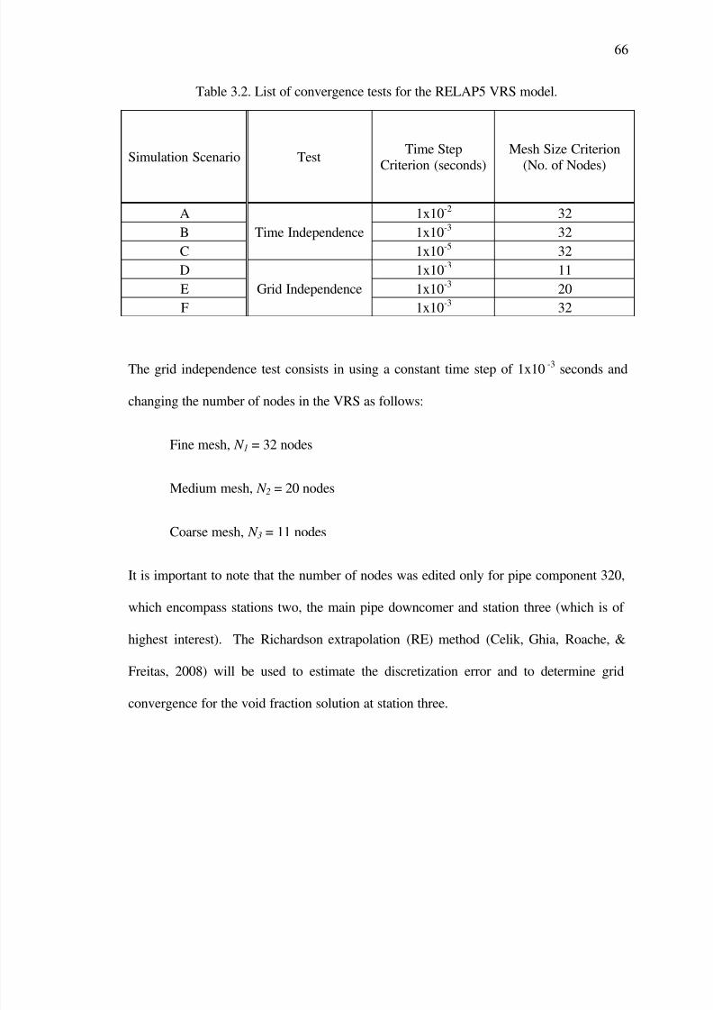
7/29/2019 Simulation and Validation of Two-component Flow in a Void Recircu
http://slidepdf.com/reader/full/simulation-and-validation-of-two-component-flow-in-a-void-recircu 82/171
66
Table 3.2. List of convergence tests for the RELAP5 VRS model.
Simulation Scenario TestTime Step
Criterion (seconds)
Mesh Size Criterion
(No. of Nodes)
A
Time Independence
1x10⁻² 32
B 1x10⁻³
32
C 1x10⁻⁵
32
D
Grid Independence
1x10⁻³
11
E 1x10⁻³
20
F 1x10⁻³ 32
The grid independence test consists in using a constant time step of 1x10⁻³ seconds and
changing the number of nodes in the VRS as follows:
Fine mesh, N 1 = 32 nodes
Medium mesh, N 2 = 20 nodes
Coarse mesh, N 3 = 11 nodes
It is important to note that the number of nodes was edited only for pipe component 320,
which encompass stations two, the main pipe downcomer and station three (which is of
highest interest). The Richardson extrapolation (RE) method (Celik, Ghia, Roache, &
Freitas, 2008) will be used to estimate the discretization error and to determine grid
convergence for the void fraction solution at station three.

7/29/2019 Simulation and Validation of Two-component Flow in a Void Recircu
http://slidepdf.com/reader/full/simulation-and-validation-of-two-component-flow-in-a-void-recircu 83/171
67
3.3.1. Time Independence Test
Figure 3.15 shows the void fraction behavior for simulation scenario one at
station three for different time steps. The time steps 1.0x10⁻²
, 1.0x10⁻³
, and 1.0x10⁻⁵
seconds can be depicted in dashed, solid and dotted lines, respectively.
Figure 3.15. Void fraction behavior for scenario one at station three for different timesteps.
During the first 65 seconds, all solutions behave similarly with an oscillatory motion,
which will be later explained under the results and discussion section. The solution for
the largest time step begins to be off-phase with respect to the other two solutions after 65
seconds. This behavior might be due to numerical calculations within RELAP5, since the
oscillation pattern seems to be the same throughout the simulation time. The relative
error was calculated using the following formula:
0.0
0.1
0.2
0.3
0.4
0.5
0.6
0.7
0.8
0 25 50 75 100 125
V o i d F
r a c t i o n
Time (s)
dt = 1.0e-2
dt = 1.0e-3
dt = 1.0e-5
7/29/2019 Simulation and Validation of Two-component Flow in a Void Recircu
http://slidepdf.com/reader/full/simulation-and-validation-of-two-component-flow-in-a-void-recircu 84/171
68
(3.1)
where VF is the void fraction at station three at a particular time, and the subscripts A and
B correspond to the largest (1.0x10⁻² seconds) and intermediate (1.0x10⁻³ seconds) time
steps, respectively. The relative error of the void fraction was computed for every second
up to 125 seconds, and an average relative error was calculated for the entire simulation
time. The average relative error between convergence scenarios A and B was
approximately 264%. This high value is a consequence of the off-phase behavior
between these two solutions. The void fraction relative error between the intermediate
(1.0x10⁻³ seconds) and smallest time steps (1.0x10⁻⁵ seconds) was found by using the
following:
(3.2)
where the subscripts B and C correspond to the intermediate and smallest time steps,
respectively. The average relative error between these convergence scenarios was found
to be approximately 35%. This comparatively low value makes sense because, unlike the
off-phase behavior between scenarios A and B, the time step solutions between scenarios
B and C are closely in phase, thus leading to a smaller relative error. In terms of
computational time, scenarios A, B and C took approximately 2 minutes, 30 minutes and
2 days, respectively. Because a greater relative error difference was obtained by using
the intermediate time step of 1.0x10⁻³ seconds when compared to total computational
time, then it was decided to use this specific time step for all simulation scenarios. In
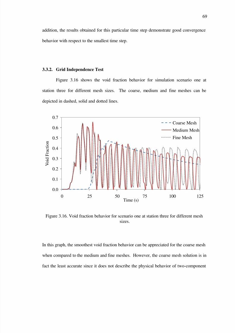
7/29/2019 Simulation and Validation of Two-component Flow in a Void Recircu
http://slidepdf.com/reader/full/simulation-and-validation-of-two-component-flow-in-a-void-recircu 85/171

7/29/2019 Simulation and Validation of Two-component Flow in a Void Recircu
http://slidepdf.com/reader/full/simulation-and-validation-of-two-component-flow-in-a-void-recircu 86/171
70
flow for the VRS experiment. The medium and fine meshes have a similar oscillating
behavior, with the exception that the solutions are not always in phase throughout the
entire simulation time. Table 3.3 shows the discretization error results for scenarios D, E
and F, which were based on the RE method.
Table 3.3. Discretization error results based on the RE method.
Parameter Value
N 1, N 2, N 3 32, 20, 11
r 21 1.37
r 32 1.48
p 3.75
ea21
192%
eext 21
135%
GCI fine21
74%
The grid refinement factor, r , is a ratio of coarse to fine mesh and is a function of the
number of nodes and the total pipe area of interest. This parameter was used to calculate
the apparent order, p using the following expressions (Celik, Ghia, Roache, & Freitas,
2008):
(3.3)
(3.4)
(3.5)
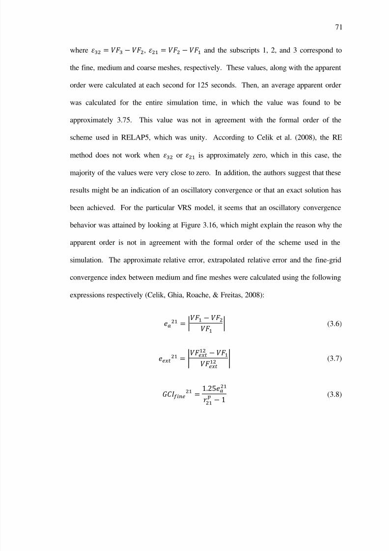
7/29/2019 Simulation and Validation of Two-component Flow in a Void Recircu
http://slidepdf.com/reader/full/simulation-and-validation-of-two-component-flow-in-a-void-recircu 87/171
71
where , and the subscripts 1, 2, and 3 correspond to
the fine, medium and coarse meshes, respectively. These values, along with the apparent
order were calculated at each second for 125 seconds. Then, an average apparent order
was calculated for the entire simulation time, in which the value was found to be
approximately 3.75. This value was not in agreement with the formal order of the
scheme used in RELAP5, which was unity. According to Celik et al. (2008), the RE
method does not work when or is approximately zero, which in this case, the
majority of the values were very close to zero. In addition, the authors suggest that these
results might be an indication of an oscillatory convergence or that an exact solution has
been achieved. For the particular VRS model, it seems that an oscillatory convergence
behavior was attained by looking at Figure 3.16, which might explain the reason why the
apparent order is not in agreement with the formal order of the scheme used in the
simulation. The approximate relative error, extrapolated relative error and the fine-grid
convergence index between medium and fine meshes were calculated using the following
expressions respectively (Celik, Ghia, Roache, & Freitas, 2008):
(3.6)
(3.7)
(3.8)
7/29/2019 Simulation and Validation of Two-component Flow in a Void Recircu
http://slidepdf.com/reader/full/simulation-and-validation-of-two-component-flow-in-a-void-recircu 88/171
72
Each of these values were then averaged for the simulation time of 125 seconds. The
relative error was found to be 192%, while the extrapolated relative error was 135%. The
fine-grid convergence index was found to be approximately 74%. These high values are
associated with the off-phase behavior seen in Figure 3.16, in addition of the high
apparent order p = 3.75. More precisely, the location of station three chosen for all
convergence scenarios slightly varied between each other due to mesh refinement.
Numerical results showed that the void fraction tends to drastically change from node to
node for this VRS model in specific. This implies that two-component flow is extremely
sensitive to pipe location and time.
As a rule of thumb, GCI should be higher than eext at an apparent order of unity.
Because the original apparent order p = 3.75 yielded a lower GCI value with respect to
eext , then it was decided to recalculate the discretization error parameters by using a
modified apparent order. Both apparent orders of unity and two were tested, but it was
found that the former value yielded extremely high discretization errors. Table 3.4
summarizes the results for the modified discretization error using p = 2.00, which is the
closest value to the formal order of the scheme used in RELAP5. In this case, the relative
and extrapolated errors were approximately 192% and the GCI is 271%, which is greater
than eext .
7/29/2019 Simulation and Validation of Two-component Flow in a Void Recircu
http://slidepdf.com/reader/full/simulation-and-validation-of-two-component-flow-in-a-void-recircu 89/171
73
Table 3.4. Modified Discretization error results based on the RE method, using p = 2.00.
Parameter Value
p 2.00
ea21 192%
eext 21
191%
GCI fine21
271%
Even though the discretization errors continue to be high, the fine mesh solution
demonstrates good convergence behavior, and more importantly, numerically describes
the behavior linked with reality. The simulation scenarios analyzed in the present study
use the finest mesh described above.
3.4. Simulation Validation, Results and Discussion
This thesis analyzes a simulation of two-component (air and water) flow in a Void
Recirculation System, where the main parameters to be considered are mass flow rates
and void fraction at stations one through four, according to Figure 3.1. Experimental
results are available from VRS tests carried at Cal Poly State University (Daza, Fong,
Rosas, & Wong, 2009) and will be used to validate the VRS model developed in
RELAP5. The purpose of analyzing mass flow rates obtained from the simulation results
is to prove that the VRS model works properly, by showing a net positive upwards flow
through the void recirculation pipe. The purpose of analyzing the void fraction is to
describe the parameter‘s behavior at all stations with respect to time and to validate the
numerical results to the VRS experiment. The simulation scenarios to be analyzed
7/29/2019 Simulation and Validation of Two-component Flow in a Void Recircu
http://slidepdf.com/reader/full/simulation-and-validation-of-two-component-flow-in-a-void-recircu 90/171
74
assume a time step of 1.0x10⁻³
seconds with the finest mesh size as described in the
convergence test section.
3.4.1. Mass Flow Rate Analysis
The mass flow rates of the VRS model for stations one, two, four and the void
recirculation pipe, for simulation scenario one (4x4x3-inch, Fr = 0.81) can be seen in
Figure 3.17. The mass flow rate in station one behaves constantly with respect to the
other sections of interest at a value of 14.5 lb/s. This behavior makes sense since there is
a constant source of water and air passing through station one. Air was injected between
20 and 35 seconds, where mass flow rate maximums can be seen for stations one, two
and four. Even though air has not yet arrived at station four, the peaking behavior is the
result of the mass conservation being calculated in RELAP5, since air is being added.
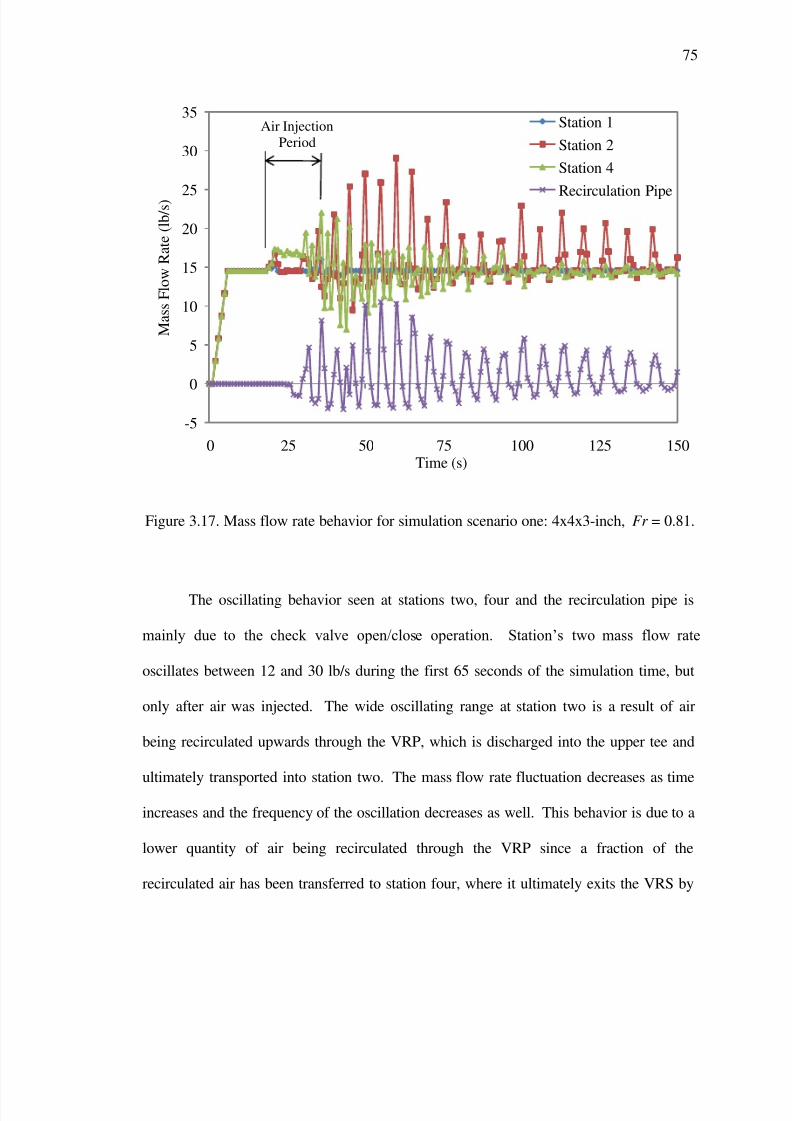
7/29/2019 Simulation and Validation of Two-component Flow in a Void Recircu
http://slidepdf.com/reader/full/simulation-and-validation-of-two-component-flow-in-a-void-recircu 91/171
75
Figure 3.17. Mass flow rate behavior for simulation scenario one: 4x4x3-inch, Fr = 0.81.
The oscillating behavior seen at stations two, four and the recirculation pipe is
mainly due to the check valve open/close operation. Station‘s two mass flow rate
oscillates between 12 and 30 lb/s during the first 65 seconds of the simulation time, but
only after air was injected. The wide oscillating range at station two is a result of air
being recirculated upwards through the VRP, which is discharged into the upper tee and
ultimately transported into station two. The mass flow rate fluctuation decreases as time
increases and the frequency of the oscillation decreases as well. This behavior is due to a
lower quantity of air being recirculated through the VRP since a fraction of the
recirculated air has been transferred to station four, where it ultimately exits the VRS by
-5
0
5
10
15
20
25
30
35
0 25 50 75 100 125 150
M a s s F l o w R a t e ( l b / s )
Time (s)
Station 1
Station 2
Station 4
Recirculation Pipe
Air Injection
Period
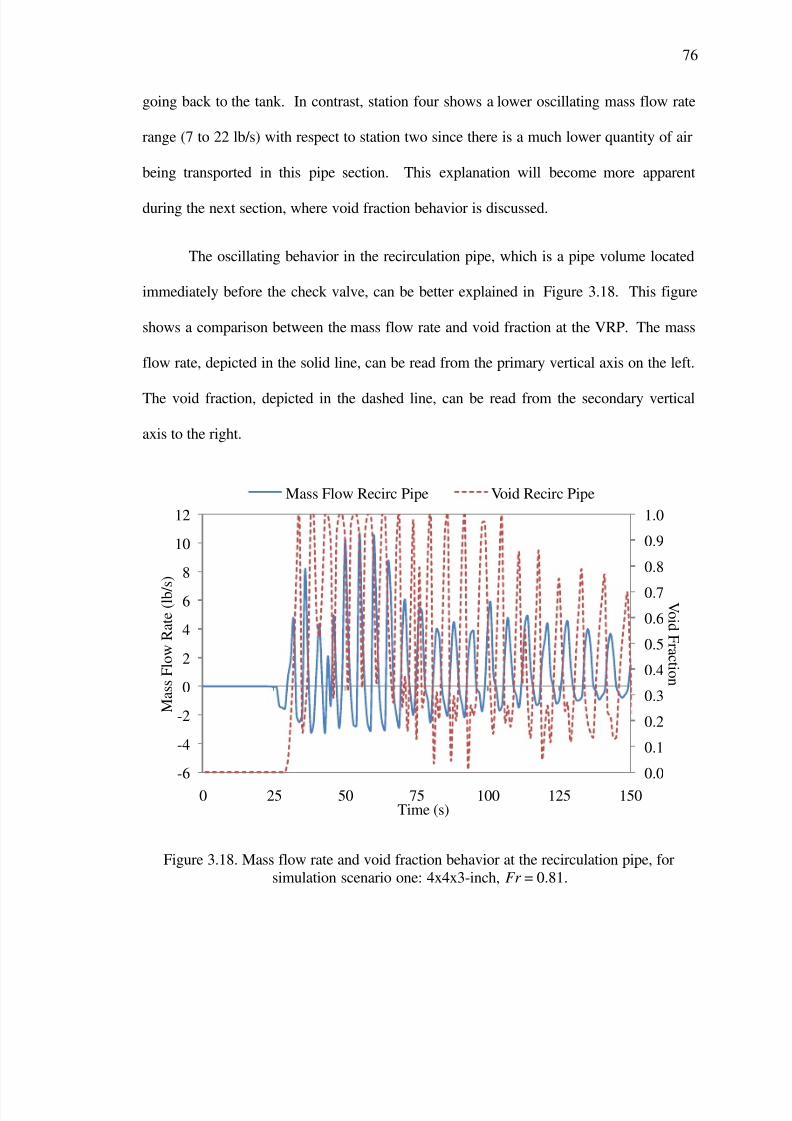
7/29/2019 Simulation and Validation of Two-component Flow in a Void Recircu
http://slidepdf.com/reader/full/simulation-and-validation-of-two-component-flow-in-a-void-recircu 92/171
76
going back to the tank. In contrast, station four shows a lower oscillating mass flow rate
range (7 to 22 lb/s) with respect to station two since there is a much lower quantity of air
being transported in this pipe section. This explanation will become more apparent
during the next section, where void fraction behavior is discussed.
The oscillating behavior in the recirculation pipe, which is a pipe volume located
immediately before the check valve, can be better explained in Figure 3.18. This figure
shows a comparison between the mass flow rate and void fraction at the VRP. The mass
flow rate, depicted in the solid line, can be read from the primary vertical axis on the left.
The void fraction, depicted in the dashed line, can be read from the secondary vertical
axis to the right.
Figure 3.18. Mass flow rate and void fraction behavior at the recirculation pipe, for
simulation scenario one: 4x4x3-inch, Fr = 0.81.
0.0
0.1
0.2
0.3
0.4
0.5
0.6
0.7
0.8
0.9
1.0
-6
-4
-2
0
2
4
6
8
10
12
0 25 50 75 100 125 150
V oi d F r a c t i on
M a s s F l o w R a t e ( l b / s )
Time (s)
Mass Flow Recirc Pipe Void Recirc Pipe

7/29/2019 Simulation and Validation of Two-component Flow in a Void Recircu
http://slidepdf.com/reader/full/simulation-and-validation-of-two-component-flow-in-a-void-recircu 93/171
77
The mass flow rate varies between -3 and 10 lb/s, where the oscillating behavior
decreases as time increases. The void fraction ranges between 0.3 and 1.0 for
approximately 75 seconds after air has been injected and later decreases towards the end
of the simulation. Note that the decreasing behavior occurs in both mass flow rate and
void fraction parameters as time increases, implying that the quantity of air recirculating
through the VRP is constantly decreasing due to a portion of air being transported to
station four. This behavior was also observed during the experiment as was described in
Section 3.1.2.5 for Froude numbers up to 1.3. Mass flow rate maximum peaks occur
when the majority of the air has passed through the check valve, resulting in a minimum
void fraction peak. On the other hand, mass flow rate minimum peaks occur when the air
accumulates before the check valve opens. Furthermore, the negative mass flow rate
peaks are an indication that the water is being forced down, by allowing the accumulation
of air until enough pressure is built to open the check valve. The simulation flow regimes
for the VRP indicate a variation between slug and annular mist. The numerical results for
scenarios four and eight, which had the highest Froude number simulated of 1.6,
indicated that recirculation ceased towards the end of the simulation by showing zero
mass flow rate and a void fraction of unity for the VRP. This settling behavior can be
seen in Figure 3.19, which is a plot comparison between the mass flow rate and void
fraction of the VRP with respect to time, for simulation scenario eight (6x6x4-inch, Fr =
1.60). This behavior makes sense since at higher Froude numbers inertia forces are high
enough to transport the air bubbles past the lower tee and into station four, thus leading to
a lower net amount of air being recirculated through the VRP. Section 3.1.2.5 describes a
similar behavior encountered during the experiment for a Froude number of 1.6.
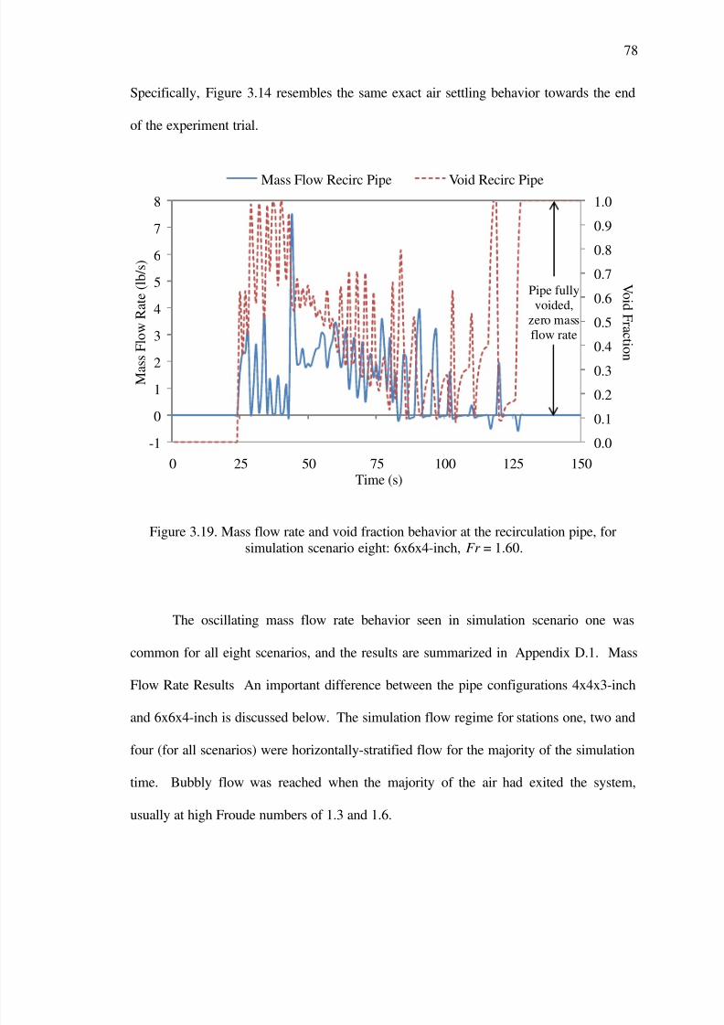
7/29/2019 Simulation and Validation of Two-component Flow in a Void Recircu
http://slidepdf.com/reader/full/simulation-and-validation-of-two-component-flow-in-a-void-recircu 94/171
78
Specifically, Figure 3.14 resembles the same exact air settling behavior towards the end
of the experiment trial.
Figure 3.19. Mass flow rate and void fraction behavior at the recirculation pipe, forsimulation scenario eight: 6x6x4-inch, Fr = 1.60.
The oscillating mass flow rate behavior seen in simulation scenario one was
common for all eight scenarios, and the results are summarized in Appendix D.1. Mass
Flow Rate Results An important difference between the pipe configurations 4x4x3-inch
and 6x6x4-inch is discussed below. The simulation flow regime for stations one, two and
four (for all scenarios) were horizontally-stratified flow for the majority of the simulation
time. Bubbly flow was reached when the majority of the air had exited the system,
usually at high Froude numbers of 1.3 and 1.6.
0.0
0.1
0.2
0.3
0.4
0.5
0.6
0.7
0.8
0.9
1.0
-1
0
1
2
3
4
5
6
7
8
0 25 50 75 100 125 150
V oi d F r a c t i on
M a s s
F l o w R a t e ( l b / s )
Time (s)
Mass Flow Recirc Pipe Void Recirc Pipe
Pipe fully
voided,
zero mass
flow rate
7/29/2019 Simulation and Validation of Two-component Flow in a Void Recircu
http://slidepdf.com/reader/full/simulation-and-validation-of-two-component-flow-in-a-void-recircu 95/171
79
One important difference seen in scenarios four (4x4x3-inch, Fr = 1.60) through
eight (6x6x4-inch, 0.81 ≤ Fr ≤ 1.60), in addition of the oscillating behavior, was the fact
that there was a steadier amount of air passing through the recirculation pipe. This effect
can be clearly seen in Figure 3.20, where the mass flow rate for stations one, two, four
and the recirculation pipe are plotted versus time. The steady behavior was a
consequence of the check valve being continuously open for a period of time, which
occurred approximately between 35 and 85 seconds for this scenario in particular. By
steady, it is meant that the oscillating behavior did not occur as drastic as was the case for
scenario one. Stations two and four were also affected by this constant source of air
coming from the VRP, but continued to oscillate after 85 seconds, once lower amounts of
air were captured in the VRP.
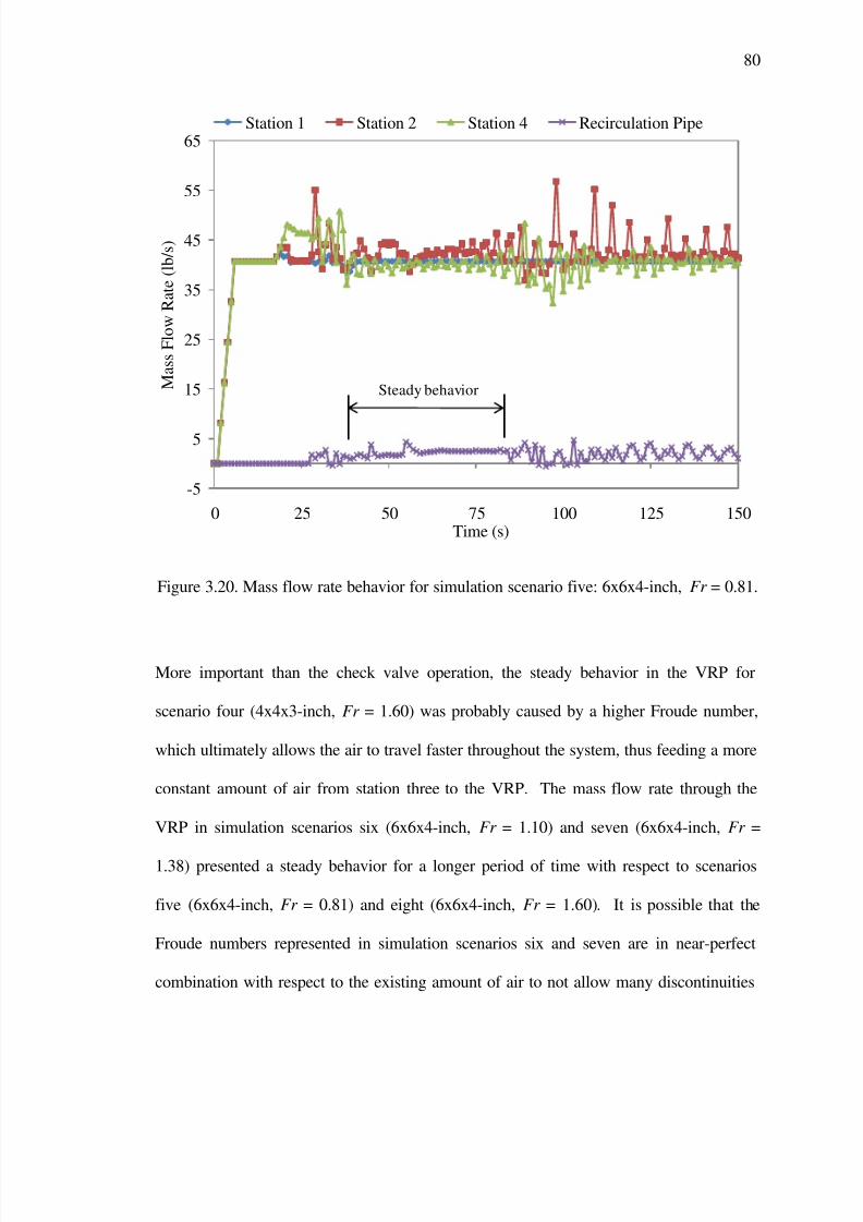
7/29/2019 Simulation and Validation of Two-component Flow in a Void Recircu
http://slidepdf.com/reader/full/simulation-and-validation-of-two-component-flow-in-a-void-recircu 96/171
80
Figure 3.20. Mass flow rate behavior for simulation scenario five: 6x6x4-inch, Fr = 0.81.
More important than the check valve operation, the steady behavior in the VRP for
scenario four (4x4x3-inch, Fr = 1.60) was probably caused by a higher Froude number,
which ultimately allows the air to travel faster throughout the system, thus feeding a more
constant amount of air from station three to the VRP. The mass flow rate through the
VRP in simulation scenarios six (6x6x4-inch, Fr = 1.10) and seven (6x6x4-inch, Fr =
1.38) presented a steady behavior for a longer period of time with respect to scenarios
five (6x6x4-inch, Fr = 0.81) and eight (6x6x4-inch, Fr = 1.60). It is possible that the
Froude numbers represented in simulation scenarios six and seven are in near-perfect
combination with respect to the existing amount of air to not allow many discontinuities
-5
5
15
25
35
45
55
65
0 25 50 75 100 125 150
M a s s F l o w R a t e ( l b / s )
Time (s)
Station 1 Station 2 Station 4 Recirculation Pipe
Steady behavior
7/29/2019 Simulation and Validation of Two-component Flow in a Void Recircu
http://slidepdf.com/reader/full/simulation-and-validation-of-two-component-flow-in-a-void-recircu 97/171
81
at the lower tee, resulting in a steadier upwards air flow. The fact that scenarios five
through eight had a steady mass flow rate behavior through the VRP, which can be
depicted in Figure D.5 through Figure D.8, was probably due to a higher cross-sectional
amount of air in the six-inch pipe, when compared to the four-inch pipe. For example, a
ten percent void fraction value in the four and six-inch pipes correspond to gas cross-
sectional areas of 1.276 in2
and 2.893 in2, respectively. Higher gas cross-sectional areas
infer that higher amounts of air are being carried throughout the system, which in turn
can prevent bubble discontinuities by allowing the air to have more surface area. This
hypothesis could be the explanation for why the mass flow rate, and thus the void fraction
did not oscillate as drastically as was the case for scenarios one through three, and it is
strongly recommended to do a more in depth analysis of this behavior. Perhaps an
analysis of the Weber number influence in horizontal flows could be performed since this
parameter compares the inertial to surface tension forces.
In short, the VRS numerical results obtained from the simulation for mass flow
rate, VRP void fraction and flow regime behavior seem to represent the physical behavior
observed during the experiment (Section 3.1.2.), thus supporting the functionality of the
VRS model.
3.4.2.
Void Fraction Analysis
The void fraction analysis will focus on stations two, three and four, which are
part of the main piping system. The purpose of analyzing the void fraction at these
sections is to show the air removal effectiveness between stations three and four, and to
7/29/2019 Simulation and Validation of Two-component Flow in a Void Recircu
http://slidepdf.com/reader/full/simulation-and-validation-of-two-component-flow-in-a-void-recircu 98/171
82
prove that the VRS model in RELAP5 works properly with respect to the experimental
observations provided in Section 3.1.2.4. In addition, the void fraction in the pipe
volume after the lower elbow will be briefly discussed. The purpose of analyzing the
void fraction in this section is to show the backward and forward motion of the air bubble
with respect to the experimental observations provided in Section 3.1.2.3.
3.4.2.1. Main Pipe Void Fraction
The void fraction behavior, for simulation scenario one (4x4x3-inch, Fr = 0.81),
at stations two, three and four can be depicted in Figure 3.21. In this graph, the
oscillating behavior is present, as was the case for the mass flow rate behavior discussed
in the previous section. This particular behavior was also due to the check valve
open/close operation, which eventually affects the entire VRS model. The air injection
procedure can be clearly reflected in station two at 20 seconds, where a steady line can be
seen for approximately 10 seconds until the void fraction starts to oscillate.
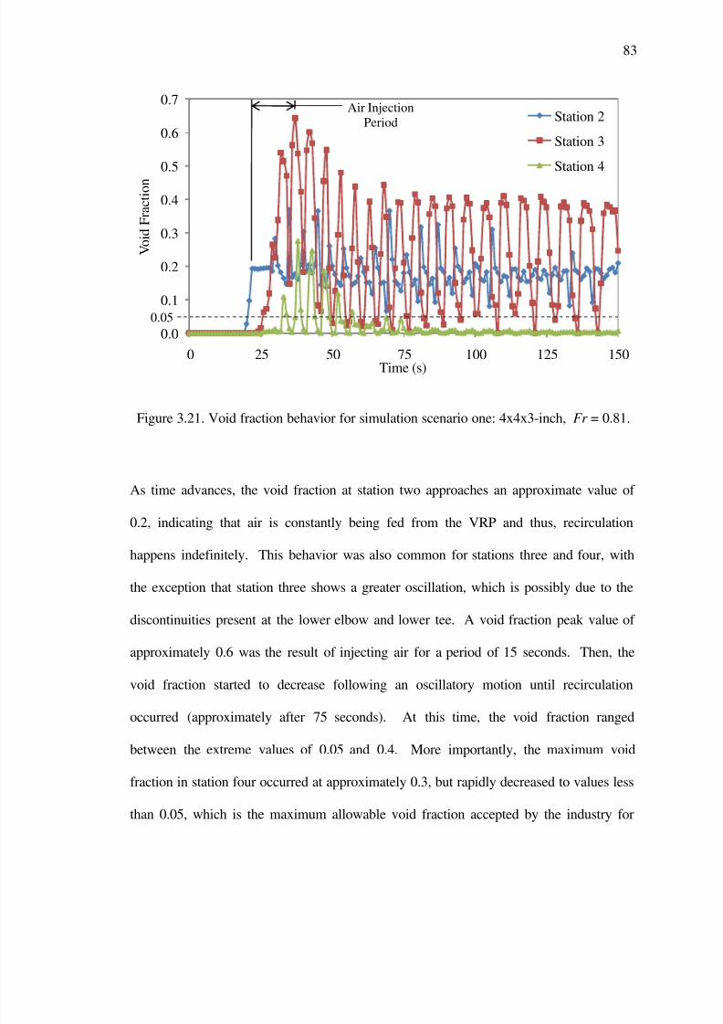
7/29/2019 Simulation and Validation of Two-component Flow in a Void Recircu
http://slidepdf.com/reader/full/simulation-and-validation-of-two-component-flow-in-a-void-recircu 99/171
83
Figure 3.21. Void fraction behavior for simulation scenario one: 4x4x3-inch, Fr = 0.81.
As time advances, the void fraction at station two approaches an approximate value of
0.2, indicating that air is constantly being fed from the VRP and thus, recirculation
happens indefinitely. This behavior was also common for stations three and four, with
the exception that station three shows a greater oscillation, which is possibly due to the
discontinuities present at the lower elbow and lower tee. A void fraction peak value of
approximately 0.6 was the result of injecting air for a period of 15 seconds. Then, the
void fraction started to decrease following an oscillatory motion until recirculation
occurred (approximately after 75 seconds). At this time, the void fraction ranged
between the extreme values of 0.05 and 0.4. More importantly, the maximum void
fraction in station four occurred at approximately 0.3, but rapidly decreased to values less
than 0.05, which is the maximum allowable void fraction accepted by the industry for
0.0
0.1
0.2
0.3
0.4
0.5
0.6
0.7
0 25 50 75 100 125 150
V o i d F r a c t i o n
Time (s)
Station 2
Station 3
Station 4
Air Injection
Period
0.05
7/29/2019 Simulation and Validation of Two-component Flow in a Void Recircu
http://slidepdf.com/reader/full/simulation-and-validation-of-two-component-flow-in-a-void-recircu 100/171
84
pipes less than 12 inches. The peaking behavior at station four was normal because of
the high initial amount of air coming from station three. The pipe configurations 4x4x3-
inch and 6x6x4-inch have a limited capacity to take large amounts of air, which explains
this initial peaking behavior. Nonetheless, the majority of the air at station three, which
is the most critical location in the VRS, was removed and recirculated throughout the
system. The void fraction seen at station four is the amount of air that was not
recirculated through the VRP, which ultimately returns to the tank. Table 3.5 shows the
numerical results for the average percent air removed between stations three and four, for
all simulation scenarios. The average amount of air for each station was measured as
void fraction, and the average percent air removed for all scenarios was greater than 88%,
which is a highly effective air removal value. The values were averaged for the period of
time until station four contained less than one percent void fraction. The percent air
removed was calculated using the following expression:
(3.9)
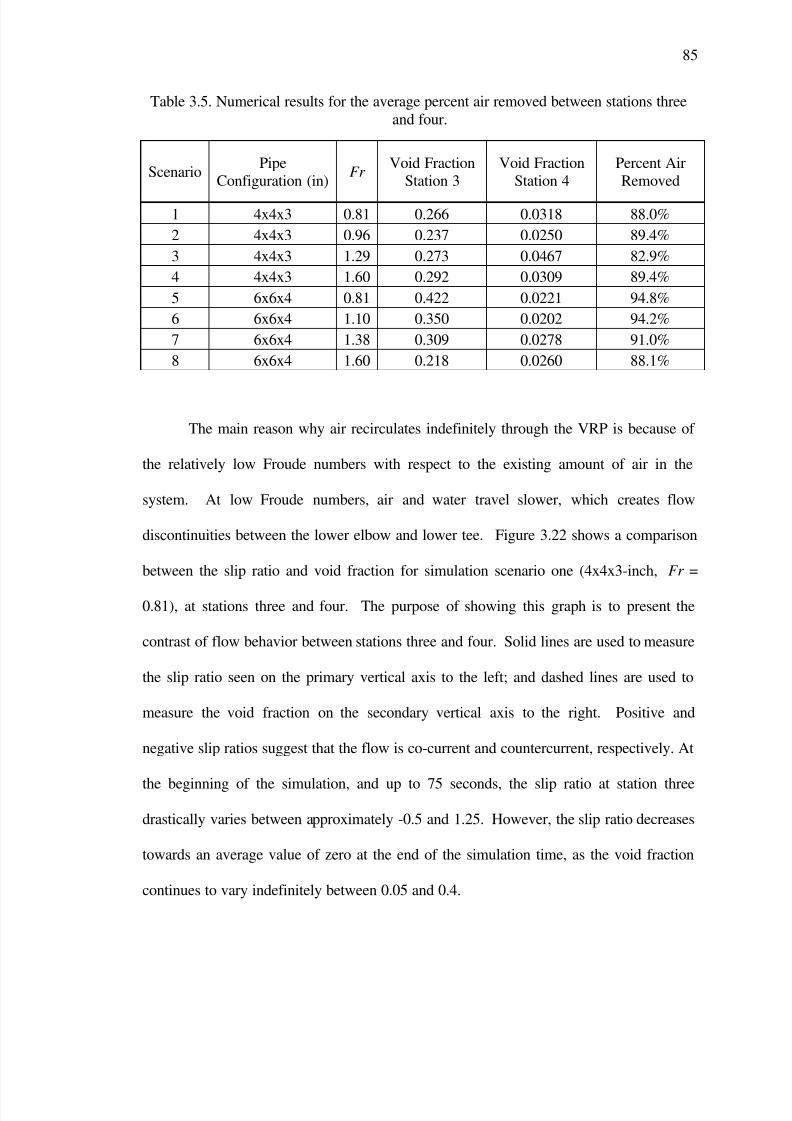
7/29/2019 Simulation and Validation of Two-component Flow in a Void Recircu
http://slidepdf.com/reader/full/simulation-and-validation-of-two-component-flow-in-a-void-recircu 101/171
85
Table 3.5. Numerical results for the average percent air removed between stations three
and four.
ScenarioPipe
Configuration (in)Fr
Void Fraction
Station 3
Void Fraction
Station 4
Percent Air
Removed
1 4x4x3 0.81 0.266 0.0318 88.0%
2 4x4x3 0.96 0.237 0.0250 89.4%
3 4x4x3 1.29 0.273 0.0467 82.9%
4 4x4x3 1.60 0.292 0.0309 89.4%
5 6x6x4 0.81 0.422 0.0221 94.8%
6 6x6x4 1.10 0.350 0.0202 94.2%
7 6x6x4 1.38 0.309 0.0278 91.0%
8 6x6x4 1.60 0.218 0.0260 88.1%
The main reason why air recirculates indefinitely through the VRP is because of
the relatively low Froude numbers with respect to the existing amount of air in the
system. At low Froude numbers, air and water travel slower, which creates flow
discontinuities between the lower elbow and lower tee. Figure 3.22 shows a comparison
between the slip ratio and void fraction for simulation scenario one (4x4x3-inch, Fr =
0.81), at stations three and four. The purpose of showing this graph is to present the
contrast of flow behavior between stations three and four. Solid lines are used to measure
the slip ratio seen on the primary vertical axis to the left; and dashed lines are used to
measure the void fraction on the secondary vertical axis to the right. Positive and
negative slip ratios suggest that the flow is co-current and countercurrent, respectively. At
the beginning of the simulation, and up to 75 seconds, the slip ratio at station three
drastically varies between approximately -0.5 and 1.25. However, the slip ratio decreases
towards an average value of zero at the end of the simulation time, as the void fraction
continues to vary indefinitely between 0.05 and 0.4.

7/29/2019 Simulation and Validation of Two-component Flow in a Void Recircu
http://slidepdf.com/reader/full/simulation-and-validation-of-two-component-flow-in-a-void-recircu 102/171
86
Figure 3.22. Slip ratio and void fraction behavior at stations three and four, for simulation
scenario one: 4x4x3-inch, Fr = 0.81.
Note that slip ratio continues to oscillate between positive and negative values even
towards the end of the simulation. This behavior suggests that air bubbles are being
continuously recirculated through the VRS, but more importantly, shows the forward and
backward motion of the air bubbles. Maximum slip ratio and void fraction values occur
at the same time, meaning that the largest possible amounts of air continue the main path
flow direction (co-current); and vice versa for minimum values in that the lowest
amounts of air travel against the direction of the main path flow (countercurrent).
0.0
0.1
0.2
0.3
0.4
0.5
0.6
0.7
0.8
0.9
1.0
-1.0
-0.5
0.0
0.5
1.0
1.5
0 25 50 75 100 125 150
V oi d F r a c t i on
S l i p R a t i o ( V g / V l )
Time (s)
Slip St. 3 Slip St. 4 Void St. 3 Void St. 4

7/29/2019 Simulation and Validation of Two-component Flow in a Void Recircu
http://slidepdf.com/reader/full/simulation-and-validation-of-two-component-flow-in-a-void-recircu 103/171
87
Conversely, station four shows that the slip ratio varies with lower magnitudes, with no
negative values, and ultimately approaches unity towards the end of the simulation. This
particular behavior suggests that air bubbles are continuously flowing co-currently
despite the amount of air.
The void fraction, as well as the slip ratio behavior seen in simulation scenario
one was common for all eight scenarios, and the results are summarized in Appendix D.2.
Void Fraction Results The simulation flow regime at station three (for all scenarios)
varied between horizontally stratified and bubbly flow. Even though not immediately
apparent, the continuous combination between these two regimes is a product of slug
flow, and matches the experimental flow regime observation previously described in
Section 3.1.2.4. However, it is important to mention that the extreme void fraction
oscillating behavior for simulation scenarios five through seven nearly disappeared
between 35 and approximately 75 seconds of the simulation. This particular behavior,
nearly disappearing oscillation, can be seen in Figure D.13 through Figure D.15, which
was caused by a steadier mass flow rate through the VRP as explained in Section 3.4.1.
A steady two-component mass flow rate implies a steady amount of air and water flow
rates, which ultimately results in a steady void fraction. Because the check valve in the
VRP remains open during this time, then a steady amount of void fraction is reflected in
stations two and three. Station four is also affected by a steady void fraction behavior
meaning that a constant amount of air is passing through without being recirculated and
ultimately exits the VRS by returning to the tank. Though, it is important to note that the
magnitudes are much lower when compared to stations two and three.

7/29/2019 Simulation and Validation of Two-component Flow in a Void Recircu
http://slidepdf.com/reader/full/simulation-and-validation-of-two-component-flow-in-a-void-recircu 104/171
88
One important distinction seen in simulation scenarios four and eight, which
correspond to a Froude number of 1.6, is that air recirculation ceases towards the end of
the simulation, as was described in the mass flow rate behavior. Figure 3.23 shows this
particular behavior for simulation scenario eight (6x6x4-inch, Fr = 1.6). The main reason
why air recirculation ceases is probably caused by a higher Froude number that
ultimately allows the air to exit the VRS at a higher rate through station four, and as a
consequence travels back to the tank. At high Froude numbers, there is less time for the
air, coming from station three, to rise through the vertical VRP. In other words, the air
bubble at high Froude numbers is traveling so fast through station three that it basically
ignores the effect of the upwards oriented lower tee, which is supposed to remove the air
by recirculating it throughout the system. From this reasoning, it is recommended to
avoid high Froude numbers to prevent large and continuous air bubbles from entering
station four, assuming the same VRS configuration is used in practice. It is possible that
other VRS configurations might have a more efficient method in recirculating the air at
high Froude numbers, and it is strongly suggested to perform further analysis by trying
different pipe diameters and/or other parts that do not require moving parts, such as the
check valve.
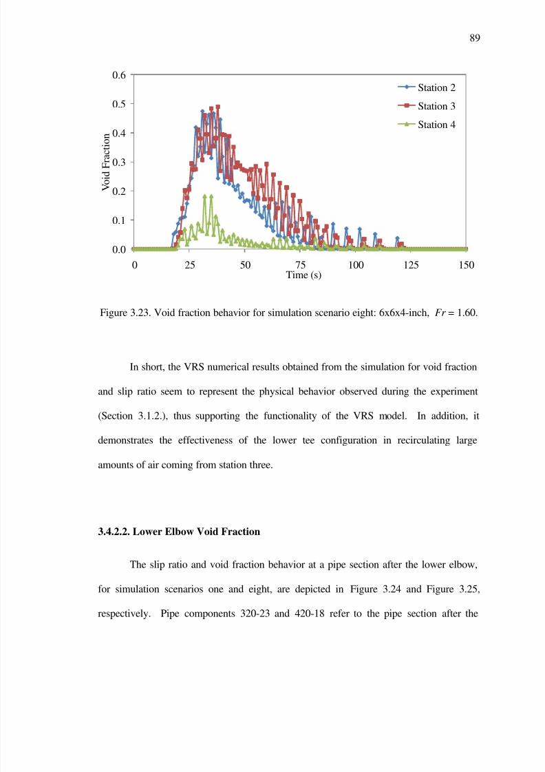
7/29/2019 Simulation and Validation of Two-component Flow in a Void Recircu
http://slidepdf.com/reader/full/simulation-and-validation-of-two-component-flow-in-a-void-recircu 105/171
89
Figure 3.23. Void fraction behavior for simulation scenario eight: 6x6x4-inch, Fr = 1.60.
In short, the VRS numerical results obtained from the simulation for void fraction
and slip ratio seem to represent the physical behavior observed during the experiment
(Section 3.1.2.), thus supporting the functionality of the VRS model. In addition, it
demonstrates the effectiveness of the lower tee configuration in recirculating large
amounts of air coming from station three.
3.4.2.2. Lower Elbow Void Fraction
The slip ratio and void fraction behavior at a pipe section after the lower elbow,
for simulation scenarios one and eight, are depicted in Figure 3.24 and Figure 3.25,
respectively. Pipe components 320-23 and 420-18 refer to the pipe section after the
0.0
0.1
0.2
0.3
0.4
0.5
0.6
0 25 50 75 100 125 150
V o i d F r a c t i o n
Time (s)
Station 2
Station 3
Station 4

7/29/2019 Simulation and Validation of Two-component Flow in a Void Recircu
http://slidepdf.com/reader/full/simulation-and-validation-of-two-component-flow-in-a-void-recircu 106/171
90
lower elbow for pipe configurations 4x4x3-inch and 6x6x4-inch, respectively. Solid and
dashed lines are used to measure slip ratio and void fraction, respectively.
Figure 3.24. Slip ratio and void fraction behavior at pipe section after lower elbow, for
simulation scenario one: 4x4x3-inch, Fr = 0.81.
Figure 3.24 shows a similar behavior as Figure 3.22 in that the slip ratio
approaches zero in an oscillatory motion towards the end of the simulation, while the
void fraction continues to oscillate between the approximate values of 0.2 and 0.5. This
behavior, while in part triggered by the check valve open/close operation, could also be
due to the relatively low Froude numbers since there is not enough flow to carry the air in
a continuous manner. In addition, the change in direction at the lower elbow contributes
to the formation of large voids due to a localized lower pressure. This in turn, creates a
discontinuity in the flow causing a slug flow behavior. According to the numerical
results, the simulated Froude numbers of 0.80, 1.0 and 1.3, indicated that the slip ratio
0.0
0.1
0.2
0.3
0.4
0.5
0.6
0.7
0.8
-0.3
-0.1
0.1
0.3
0.5
0.7
0.9
1.1
1.31.5
0 25 50 75 100 125 150
V oi d F r a c t i on
S l i p R a t i o ( V g / V l )
Time (s)
Slip 320-23
Void 320-23
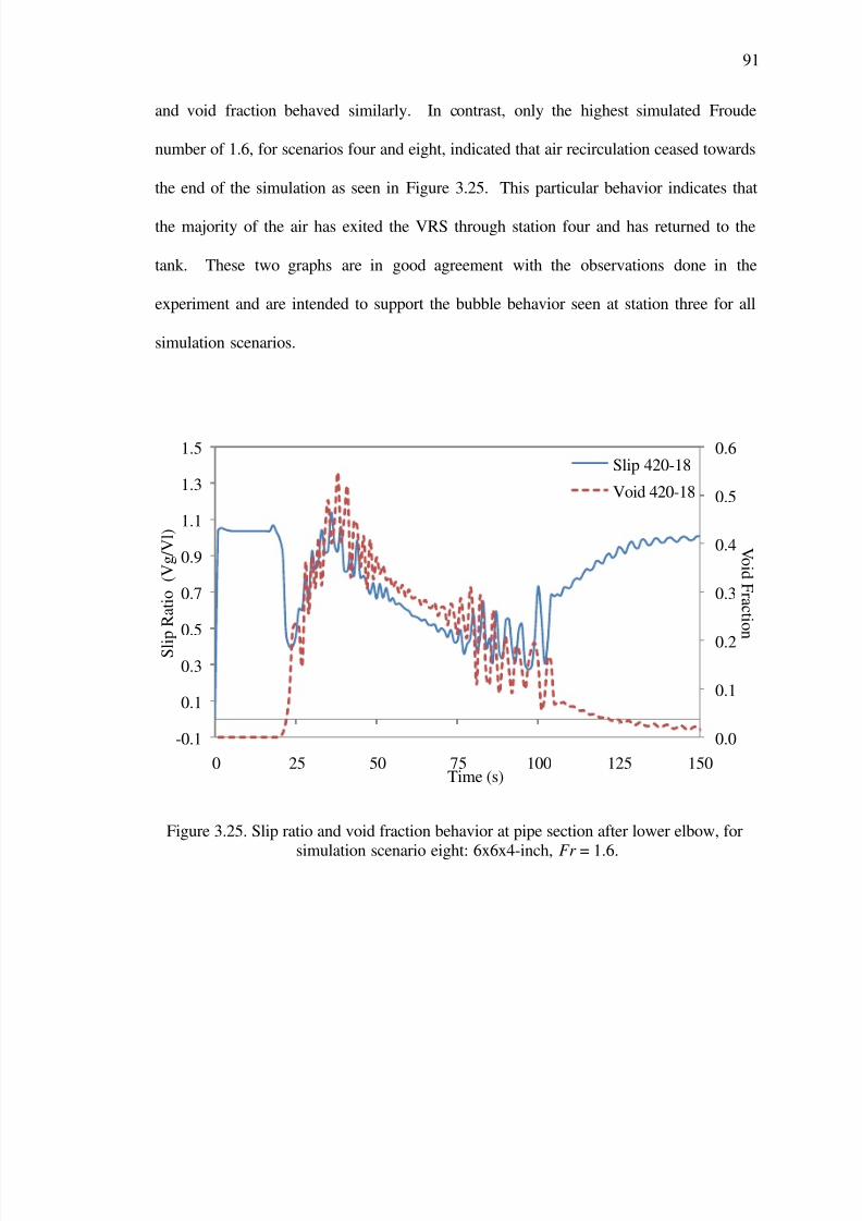
7/29/2019 Simulation and Validation of Two-component Flow in a Void Recircu
http://slidepdf.com/reader/full/simulation-and-validation-of-two-component-flow-in-a-void-recircu 107/171
91
and void fraction behaved similarly. In contrast, only the highest simulated Froude
number of 1.6, for scenarios four and eight, indicated that air recirculation ceased towards
the end of the simulation as seen in Figure 3.25. This particular behavior indicates that
the majority of the air has exited the VRS through station four and has returned to the
tank. These two graphs are in good agreement with the observations done in the
experiment and are intended to support the bubble behavior seen at station three for all
simulation scenarios.
Figure 3.25. Slip ratio and void fraction behavior at pipe section after lower elbow, for
simulation scenario eight: 6x6x4-inch, Fr = 1.6.
0.0
0.1
0.2
0.3
0.4
0.5
0.6
-0.1
0.1
0.3
0.5
0.7
0.9
1.1
1.3
1.5
0 25 50 75 100 125 150
V oi d F r a c t i o
n
S l i p R a t i o ( V g / V l )
Time (s)
Slip 420-18
Void 420-18

7/29/2019 Simulation and Validation of Two-component Flow in a Void Recircu
http://slidepdf.com/reader/full/simulation-and-validation-of-two-component-flow-in-a-void-recircu 108/171
92
3.4.3. Simulation and Experimental Void Fraction Validation
Now that the VRS model has been verified with respect to experimental
observations and plausible explanations for the different flow behaviors seen in the pipe
sections of interest, the validation between simulation and experimental void fraction
results can be analyzed. More specifically, time-averaged void fraction values will be
compared in order to validate the VRS model built in RELAP5. Since the void fraction
experimental results were averaged for a period of approximately 120 seconds for each
scenario, which represents the time at which station four reached a void fraction less than
one percent, then it makes sense to average the void fraction numerical results for the
period of time that satisfies the void fraction condition at station four. Figure 3.26 shows
the void fraction validation between experimental and numerical (model) results, at
stations one through four, for simulation scenario one (4x4x3-inch, Fr = 0.81).

7/29/2019 Simulation and Validation of Two-component Flow in a Void Recircu
http://slidepdf.com/reader/full/simulation-and-validation-of-two-component-flow-in-a-void-recircu 109/171
93
Figure 3.26. Void fraction validation of the VRS model for simulation scenario one:
4x4x3-inch, Fr = 0.81.
The bars shown in this graph actually represent uncertainty ranges, rather than error bars,
since insufficient experimental data was available for a thorough statistical analysis.
Solid and dashed bars represent experimental and model uncertainty ranges, respectively.
The experimental uncertainty associated with the void fraction at each station was
approximately ±0.5 inches, since this value was much larger than the other parameters
(length and pipe diameter uncertainty) used for general uncertainty propagation. This
specific value was determined by visually inspecting the length variation (in inches) of
the void fraction. Figure 3.27 shows a schematic of a pipe partially filled with water,
along with the variables used to calculate the void fraction. The air phase is occupying
the top portion of the inner pipe diameter, while the water phase is occupying the bottom
0.0
0.1
0.2
0.3
0.4
0.5
0.6
0.7
0 1 2 3 4 5
V o i d F r a c t i o n
Station No.
Experimental
Model
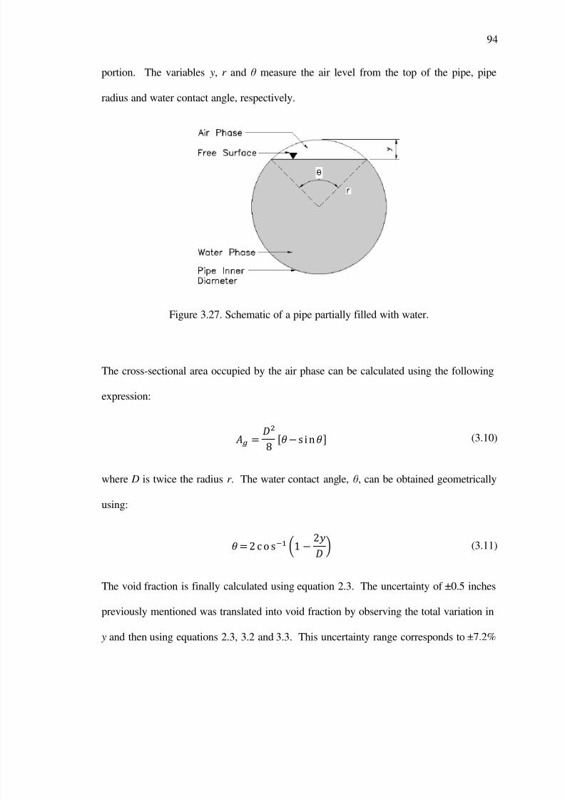
7/29/2019 Simulation and Validation of Two-component Flow in a Void Recircu
http://slidepdf.com/reader/full/simulation-and-validation-of-two-component-flow-in-a-void-recircu 110/171
94
portion. The variables y, r and θ measure the air level from the top of the pipe, pipe
radius and water contact angle, respectively.
Figure 3.27. Schematic of a pipe partially filled with water.
The cross-sectional area occupied by the air phase can be calculated using the following
expression:
(3.10)
where D is twice the radius r . The water contact angle, θ , can be obtained geometrically
using:
(3.11)
The void fraction is finally calculated using equation 2.3. The uncertainty of ±0.5 inches
previously mentioned was translated into void fraction by observing the total variation in
y and then using equations 2.3, 3.2 and 3.3. This uncertainty range corresponds to ±7.2%
7/29/2019 Simulation and Validation of Two-component Flow in a Void Recircu
http://slidepdf.com/reader/full/simulation-and-validation-of-two-component-flow-in-a-void-recircu 111/171
95
and ±3.9% void fration for four inch and six inch pipe diameters, respectively. As a
result, all void fractions calculated for the four inch pipe had greater uncertainty values.
For this particular scenario validation, the numerical results over predicted the
experimental results at stations one and four, and under predicted the experimental results
at stations two and three. Nonetheless, the uncertainty ranges of both experimental and
model results at each station overlap with each other, meaning that any of the values
could fall in this range at any particular time. Uncertainty overlapping not only proves
that the model resembles realistic behavior, but also validates the VRS model built in
RELAP5.
In regards to the remaining simulation scenarios, the void fraction validation was
achieved for the majority of Froude numbers and stations of interest. A summary of the
validation plots can be seen in Appendix E – VRS Simulation and Experimental Void
Fraction Validation for further reference. However, it is important to note that the
validation at station three, which is of highest significance, was not achieved in the
following three scenarios: four, seven and eight. It is believed that the apparent under-
prediction of the numerical results for these scenarios was not the cause for a non-
numerical validation. On the contrary, it is believed the all void fraction values obtained
from the experiment were too conservative and thus over-predicted the actual value.
7/29/2019 Simulation and Validation of Two-component Flow in a Void Recircu
http://slidepdf.com/reader/full/simulation-and-validation-of-two-component-flow-in-a-void-recircu 112/171
96
Chapter 4. CONCLUSIONS AND RECOMMENDATIONS
4.1. Conclusions
In conclusion, the objectives of this thesis were accomplished by (1) simulating a
Void Recirculation System model using RELAP5 and investigating the behavior of two-
component flow by means of analyzing mass flow rates, void fraction and slip ratios; and
(2) successfully validating its results with respect to experimental results and
observations.
The Void Recirculation System model, simulated in RELAP5, was successfully
validated against experimental results using the void fraction parameter. A total of eight
simulation scenarios were analyzed using two different pipe configurations (4x4x3-inch
and 6x6x4-inch), and four Froude numbers (0.80, 1.0, 1.3 and 1.6). The void fraction
numerical results obtained from RELAP5 were in good agreement with experimental
results and represent the physical behavior seen during the Void Recirculation System
experiment.
The numerical results confirmed that air recirculation is more effective at Froude
numbers of 0.80, 1.0 and 1.3, which resemble experimental observations. At these
Froude numbers, recirculation occurs indefinitely, or for a long period of time, since air
does not travel fast enough to exit the Void Recirculation System. Conversely, the
numerical results showed that air recirculation occurs for a short period of time, and
ceases towards the end of the simulation at the highest Froude number simulated of 1.6.
For this reason, high Froude numbers, and thus high flow rates, should be avoided if air is
to be recirculated more effectively. The void fraction and mass flow rate oscillating

7/29/2019 Simulation and Validation of Two-component Flow in a Void Recircu
http://slidepdf.com/reader/full/simulation-and-validation-of-two-component-flow-in-a-void-recircu 113/171
7/29/2019 Simulation and Validation of Two-component Flow in a Void Recircu
http://slidepdf.com/reader/full/simulation-and-validation-of-two-component-flow-in-a-void-recircu 114/171
98
at elbows and tees is recommended to better understand the scalability of the Void
Recirculation System for different pipe diameters.
Finally, the modeling of other pipe configurations (using the VRS model) that
recirculate air is strongly suggested, since it could help to decide what diameters are
appropriate for each application. In addition, it is recommended to model other VRS
ideas that could improve air recirculation by not having to use moving parts, such as a
check valve. These recommended computational efforts can expand the validity of the
VRS model, lower experiment expenses and could help identify if the VRS solution is
suitable for a particular application.
7/29/2019 Simulation and Validation of Two-component Flow in a Void Recircu
http://slidepdf.com/reader/full/simulation-and-validation-of-two-component-flow-in-a-void-recircu 115/171
99
Bibliography
Baker, G., Clark, W. W., Azzopardi, B. J., & Wilson, J. A. (2008). Transient effects in gas – liquid phase separation at a pair of T-junctions. Chemical Engineering Science , 63, 968-
976.
Celik, I. B., Ghia, U., Roache, P. J., & Freitas, C. J. (2008). Procedure for Estimation and
Reporting of Uncertainty Due to Discretization in CFD Applications. Journal of Fluids
Engineering , 1-15.
Chisholm, D. (1968). Prediction of pressure losses at changes of section, bends and throttling
devices. NEL Report No 388. Glasgow: National Engineering Laboratory.
Chisholm, D. (1983). Two-Phase flow in pipelines and heat exchangers. New York: Longman
Inc.
Crane Corporation. (1988). Flow of Fluids through Valves, Fittings, and Pipe. Stamford: Crane
Corporation.
Daza, O. E., Fong, M. J., Rosas, R., & Wong, B. S. (2009). Void Recirculation system. San Luis
Obispo: Cal Poly State University.
de Sampaio, P. A., Faccini, J. L., & Su, J. (2008). Modeling of stratified gas-liquid two-phase
flow in horizontal circular pipes. International Journal of Heat and Mass Transfer , 51,2752-2761.
Diablo Canyon Power Plant, PG&E. (2009, January 24). Void Recirculation Device. AvilaBeach, CA.
Flow Regime Sample Movies. (n.d.). Retrieved April 19, 2011, from http://ct-
cr4.chem.uva.nl/SingleCapillary/sample_videos_flow_regime.html
Fox, R. W., McDonald, A. T., & Pritchard, P. J. (2006). Introduction to Fluid Mechanics. John
Wiley & Sons, Inc.
Ghiaasiaan, S. M. (2008). Two-Phase Flow, Boiling, and Condensation in Conventional and
Miniature Systems. New York: Cambridge University Press.
Groudev, P. P., & Gencheva, R. V. (2004). Relap5/mod3.2 investigation of main loop isolating
valves in case of SGTR in VVER440/V230. Annals of Nuclear Energy , 31, 1583-1613.
Institute of Nuclear Power Operations. (2010). How Engineering can Manage Gas
Accumulation. Training Module 2 . United States of America: INPO.
Ishii, M. (1975). Thermo-Fluid Dynamic Theory of Two-Phase Flow. Paris: Eyrolles.
Ishii, M., & Mishima, K. (1984). Two-Fluid model and hydrodynamic constitutive relations.
Nuclear Engineering and Design , 82 (2-3), 107-126.

7/29/2019 Simulation and Validation of Two-component Flow in a Void Recircu
http://slidepdf.com/reader/full/simulation-and-validation-of-two-component-flow-in-a-void-recircu 116/171
100
Jain, S. C. (2001). Open-Channel Flow. New York, New York, USA: John Wiley & Sons.
Kadri, U., Mudde, R. F., Oliemans, R., Bonizzi, M., & Andreussi, P. (2009). Prediction of the
transition from stratified to slug flow or roll-waves in gas – liquid horizontal pipes.
International Journal of Multiphase Flow 35 , 1001-1010.
Kaliatka, A., & Uspuras, E. (2008). Development and testing of RBMK-1500 model for BDBAanalysis employing RELAP/SCDAPSIM code. Annals of Nuclear Energy , 35, 997-992.
Margaris, D. P. (2007). T-junction separation modelling in gas – liquid two-phase flow. Chemical
Engineering and Processing , 46 , 150-158.
Marshall, J. (2003). Two-Phase Flow. San Luis Obispo: Cal Poly State University.
Newton, C., & Behnia, M. (2001). A numerical model of stratified wavy gas-liquid pipe flow.Chemical Engineering Science , 56 , 6851-6861.
Nuclear Regulatory Commission. (2010). Resolution of Generic Safety Issues: Issue 193: BWR ECCS Suction Concerns Description (NUREG-0933, Main Report with Supplements 1-
33). Washington: Nuclear Regulatory Commission.
Nuclear Regulatory Commission. (2006, September 21). U.S. NRC Information Notices.
Retrieved from U.S. NRC: http://www.nrc.gov/reading-rm/doc-collections/gen-comm/info-notices/2006/in200621.pdf
Ottens, M., Hoefsloot, H. C., & Hamersma, P. J. (2001). Transient gas}liquid #ow in horizontalT-junctions. Chemical Engineering Science , 56 , 43-55.
Phillips, B. E. (2003). RHR Water Hammer Simulation and Evaluation. San Luis Obispo: Cal
Poly State University.
RELAP5/MOD3.2. (1995). Code Manual Volume I: Code Structure, System Models, and
Solution Methods (Vol. I). Idaho Falls: NUREG/CR-5535.
RELAP5/MOD3.2. (1995). Code Manual Volume II: User's Guide and Input Requirements.
Idaho Falls: NUREG/CR-5535.
Sarrette, C., & Bestion, D. (2003). Study of release of nitrogen gas dissolved in water during
depressurisation — application to primary circuit of PWR. Nuclear Engineering and
Design , 224, 337-358.
Sidi-Ali, K., & Gatignol, R. (2010). Interfacial friction factor determination using CFDsimulations in a horizontal stratified two-phaseflow. Chemical Engineering Science , 65,
5160-5169.
Spears Manufacturing Company. (2010, February 1). PVC White Schedule 40 Fittings, Unions,
& Saddles. Technical Information Weights & Dimensions . Spears Manufacturing
Company.

7/29/2019 Simulation and Validation of Two-component Flow in a Void Recircu
http://slidepdf.com/reader/full/simulation-and-validation-of-two-component-flow-in-a-void-recircu 117/171
101
Taitel, Y., & Dukler, A. E. (1976). A theoretical approach to the Lockhart-Martinelli correlation
for stratified flow. International Journal of Multiphase flow , 2, 591-595.
Wallis, G. B. (1969). One-Dimensional Two-Phase Flow. New York: McGraw-Hill, Inc.
Westinghouse Electric Company LLC. (2011). Investigation of Simplified Equation for Gas
Transport. Cranberry Township: Westinghouse Electric Company LLC.
Westinghouse Electric Company, LLC. (2010). Technical Basis for Gas Transport to the Pump
Suction. Cranberry Township: Westinghouse Electric Company, LLC.
Woods, B. D., & Hanratty, T. J. (1999). Influence of Froude number on physical processesdetermining frequency of slugging in horizontal gas-liquid flows. International Journal
of Multiphase Flow 25 , 1195-1223.

7/29/2019 Simulation and Validation of Two-component Flow in a Void Recircu
http://slidepdf.com/reader/full/simulation-and-validation-of-two-component-flow-in-a-void-recircu 118/171
102
Appendix A – VRS Piping Drawings
F i g u r e A . 1 . 4 x 4 x
3 - i n c h V R S P i p e C o n f i g u r a t i o n
D r a w i n g .
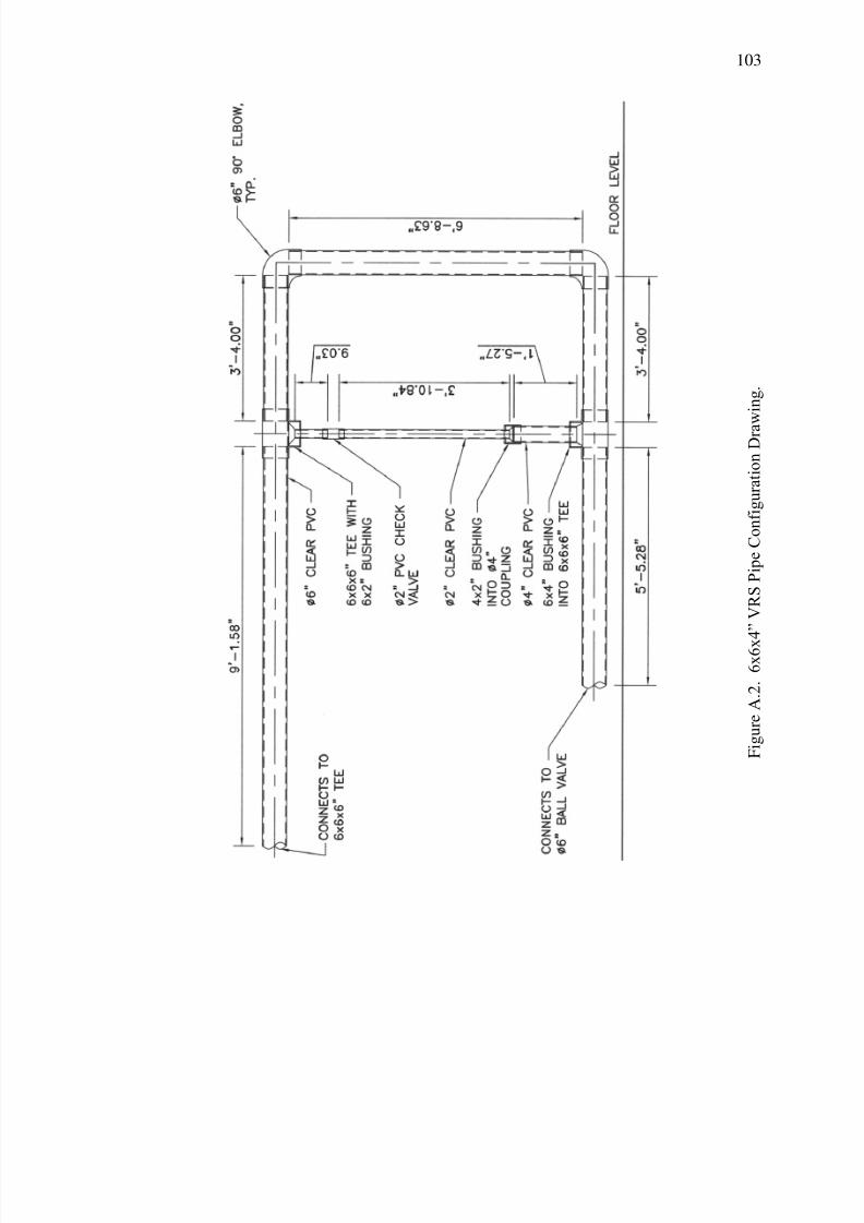
7/29/2019 Simulation and Validation of Two-component Flow in a Void Recircu
http://slidepdf.com/reader/full/simulation-and-validation-of-two-component-flow-in-a-void-recircu 119/171
103
F i g u r e A . 2 . 6 x 6 x
4 ‖ V R S P i p e C o n f i g u r a t i o n D r a
w i n g .
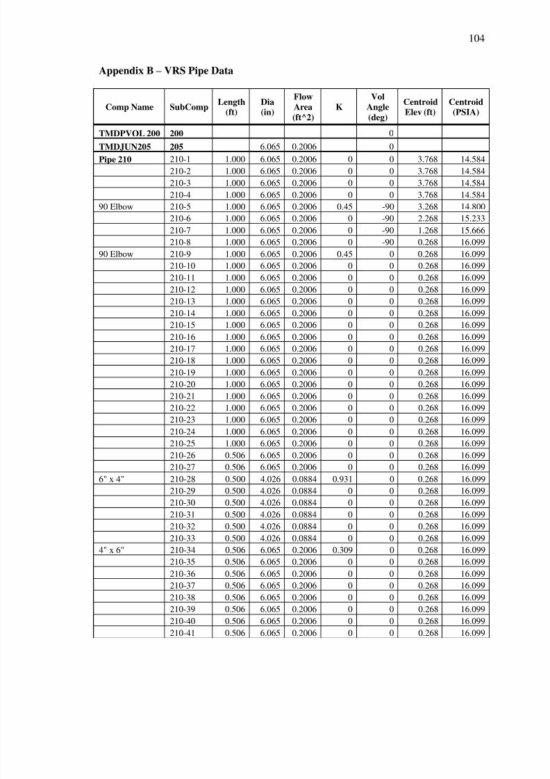
7/29/2019 Simulation and Validation of Two-component Flow in a Void Recircu
http://slidepdf.com/reader/full/simulation-and-validation-of-two-component-flow-in-a-void-recircu 120/171
104
Appendix B – VRS Pipe Data
Comp Name SubCompLength
(ft)
Dia
(in)
Flow
Area
(ft^2)
K
Vol
Angle
(deg)
Centroid
Elev (ft)
Centroid
(PSIA)
TMDPVOL 200 200 0TMDJUN205 205 6.065 0.2006 0
Pipe 210 210-1 1.000 6.065 0.2006 0 0 3.768 14.584
210-2 1.000 6.065 0.2006 0 0 3.768 14.584
210-3 1.000 6.065 0.2006 0 0 3.768 14.584
210-4 1.000 6.065 0.2006 0 0 3.768 14.584
90 Elbow 210-5 1.000 6.065 0.2006 0.45 -90 3.268 14.800
210-6 1.000 6.065 0.2006 0 -90 2.268 15.233
210-7 1.000 6.065 0.2006 0 -90 1.268 15.666
210-8 1.000 6.065 0.2006 0 -90 0.268 16.099
90 Elbow 210-9 1.000 6.065 0.2006 0.45 0 0.268 16.099
210-10 1.000 6.065 0.2006 0 0 0.268 16.099
210-11 1.000 6.065 0.2006 0 0 0.268 16.099
210-12 1.000 6.065 0.2006 0 0 0.268 16.099
210-13 1.000 6.065 0.2006 0 0 0.268 16.099
210-14 1.000 6.065 0.2006 0 0 0.268 16.099
210-15 1.000 6.065 0.2006 0 0 0.268 16.099
210-16 1.000 6.065 0.2006 0 0 0.268 16.099
210-17 1.000 6.065 0.2006 0 0 0.268 16.099
210-18 1.000 6.065 0.2006 0 0 0.268 16.099
210-19 1.000 6.065 0.2006 0 0 0.268 16.099
210-20 1.000 6.065 0.2006 0 0 0.268 16.099
210-21 1.000 6.065 0.2006 0 0 0.268 16.099
210-22 1.000 6.065 0.2006 0 0 0.268 16.099210-23 1.000 6.065 0.2006 0 0 0.268 16.099
210-24 1.000 6.065 0.2006 0 0 0.268 16.099
210-25 1.000 6.065 0.2006 0 0 0.268 16.099
210-26 0.506 6.065 0.2006 0 0 0.268 16.099
210-27 0.506 6.065 0.2006 0 0 0.268 16.099
6" x 4" 210-28 0.500 4.026 0.0884 0.931 0 0.268 16.099
210-29 0.500 4.026 0.0884 0 0 0.268 16.099
210-30 0.500 4.026 0.0884 0 0 0.268 16.099
210-31 0.500 4.026 0.0884 0 0 0.268 16.099
210-32 0.500 4.026 0.0884 0 0 0.268 16.099
210-33 0.500 4.026 0.0884 0 0 0.268 16.099
4" x 6" 210-34 0.506 6.065 0.2006 0.309 0 0.268 16.099
210-35 0.506 6.065 0.2006 0 0 0.268 16.099
210-36 0.506 6.065 0.2006 0 0 0.268 16.099
210-37 0.506 6.065 0.2006 0 0 0.268 16.099
210-38 0.506 6.065 0.2006 0 0 0.268 16.099
210-39 0.506 6.065 0.2006 0 0 0.268 16.099
210-40 0.506 6.065 0.2006 0 0 0.268 16.099
210-41 0.506 6.065 0.2006 0 0 0.268 16.099
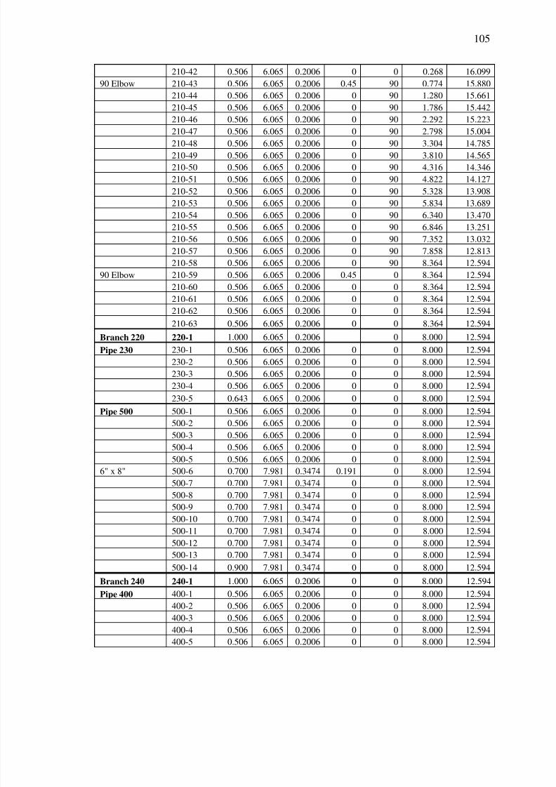
7/29/2019 Simulation and Validation of Two-component Flow in a Void Recircu
http://slidepdf.com/reader/full/simulation-and-validation-of-two-component-flow-in-a-void-recircu 121/171
105
210-42 0.506 6.065 0.2006 0 0 0.268 16.099
90 Elbow 210-43 0.506 6.065 0.2006 0.45 90 0.774 15.880
210-44 0.506 6.065 0.2006 0 90 1.280 15.661
210-45 0.506 6.065 0.2006 0 90 1.786 15.442
210-46 0.506 6.065 0.2006 0 90 2.292 15.223
210-47 0.506 6.065 0.2006 0 90 2.798 15.004
210-48 0.506 6.065 0.2006 0 90 3.304 14.785
210-49 0.506 6.065 0.2006 0 90 3.810 14.565
210-50 0.506 6.065 0.2006 0 90 4.316 14.346
210-51 0.506 6.065 0.2006 0 90 4.822 14.127
210-52 0.506 6.065 0.2006 0 90 5.328 13.908
210-53 0.506 6.065 0.2006 0 90 5.834 13.689
210-54 0.506 6.065 0.2006 0 90 6.340 13.470
210-55 0.506 6.065 0.2006 0 90 6.846 13.251
210-56 0.506 6.065 0.2006 0 90 7.352 13.032
210-57 0.506 6.065 0.2006 0 90 7.858 12.813
210-58 0.506 6.065 0.2006 0 90 8.364 12.594
90 Elbow 210-59 0.506 6.065 0.2006 0.45 0 8.364 12.594210-60 0.506 6.065 0.2006 0 0 8.364 12.594
210-61 0.506 6.065 0.2006 0 0 8.364 12.594
210-62 0.506 6.065 0.2006 0 0 8.364 12.594
210-63 0.506 6.065 0.2006 0 0 8.364 12.594
Branch 220 220-1 1.000 6.065 0.2006 0 8.000 12.594
Pipe 230 230-1 0.506 6.065 0.2006 0 0 8.000 12.594
230-2 0.506 6.065 0.2006 0 0 8.000 12.594
230-3 0.506 6.065 0.2006 0 0 8.000 12.594
230-4 0.506 6.065 0.2006 0 0 8.000 12.594
230-5 0.643 6.065 0.2006 0 0 8.000 12.594
Pipe 500 500-1 0.506 6.065 0.2006 0 0 8.000 12.594500-2 0.506 6.065 0.2006 0 0 8.000 12.594
500-3 0.506 6.065 0.2006 0 0 8.000 12.594
500-4 0.506 6.065 0.2006 0 0 8.000 12.594
500-5 0.506 6.065 0.2006 0 0 8.000 12.594
6" x 8" 500-6 0.700 7.981 0.3474 0.191 0 8.000 12.594
500-7 0.700 7.981 0.3474 0 0 8.000 12.594
500-8 0.700 7.981 0.3474 0 0 8.000 12.594
500-9 0.700 7.981 0.3474 0 0 8.000 12.594
500-10 0.700 7.981 0.3474 0 0 8.000 12.594
500-11 0.700 7.981 0.3474 0 0 8.000 12.594
500-12 0.700 7.981 0.3474 0 0 8.000 12.594
500-13 0.700 7.981 0.3474 0 0 8.000 12.594
500-14 0.900 7.981 0.3474 0 0 8.000 12.594
Branch 240 240-1 1.000 6.065 0.2006 0 0 8.000 12.594
Pipe 400 400-1 0.506 6.065 0.2006 0 0 8.000 12.594
400-2 0.506 6.065 0.2006 0 0 8.000 12.594
400-3 0.506 6.065 0.2006 0 0 8.000 12.594
400-4 0.506 6.065 0.2006 0 0 8.000 12.594
400-5 0.506 6.065 0.2006 0 0 8.000 12.594
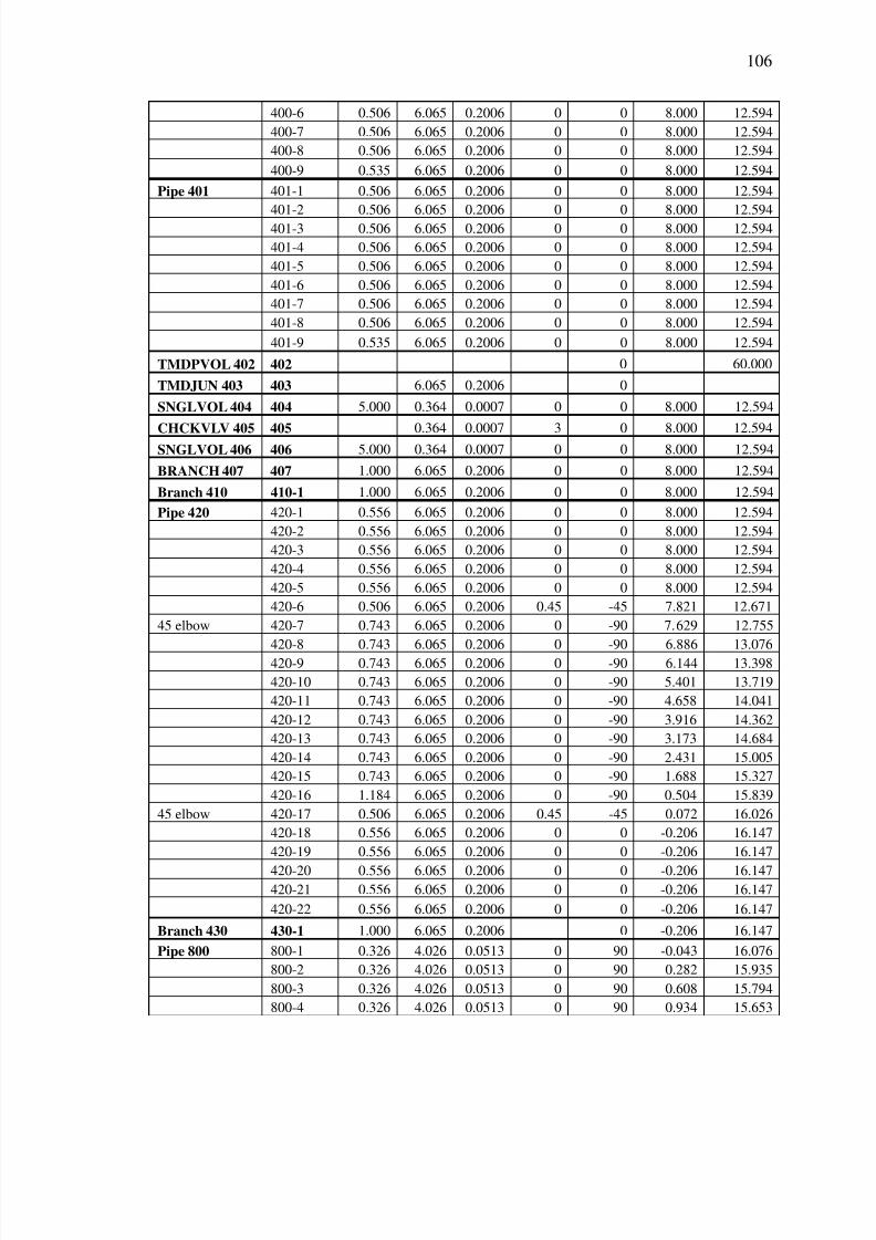
7/29/2019 Simulation and Validation of Two-component Flow in a Void Recircu
http://slidepdf.com/reader/full/simulation-and-validation-of-two-component-flow-in-a-void-recircu 122/171
106
400-6 0.506 6.065 0.2006 0 0 8.000 12.594
400-7 0.506 6.065 0.2006 0 0 8.000 12.594
400-8 0.506 6.065 0.2006 0 0 8.000 12.594
400-9 0.535 6.065 0.2006 0 0 8.000 12.594
Pipe 401 401-1 0.506 6.065 0.2006 0 0 8.000 12.594
401-2 0.506 6.065 0.2006 0 0 8.000 12.594401-3 0.506 6.065 0.2006 0 0 8.000 12.594
401-4 0.506 6.065 0.2006 0 0 8.000 12.594
401-5 0.506 6.065 0.2006 0 0 8.000 12.594
401-6 0.506 6.065 0.2006 0 0 8.000 12.594
401-7 0.506 6.065 0.2006 0 0 8.000 12.594
401-8 0.506 6.065 0.2006 0 0 8.000 12.594
401-9 0.535 6.065 0.2006 0 0 8.000 12.594
TMDPVOL 402 402 0 60.000
TMDJUN 403 403 6.065 0.2006 0
SNGLVOL 404 404 5.000 0.364 0.0007 0 0 8.000 12.594
CHCKVLV 405 405 0.364 0.0007 3 0 8.000 12.594SNGLVOL 406 406 5.000 0.364 0.0007 0 0 8.000 12.594
BRANCH 407 407 1.000 6.065 0.2006 0 0 8.000 12.594
Branch 410 410-1 1.000 6.065 0.2006 0 0 8.000 12.594
Pipe 420 420-1 0.556 6.065 0.2006 0 0 8.000 12.594
420-2 0.556 6.065 0.2006 0 0 8.000 12.594
420-3 0.556 6.065 0.2006 0 0 8.000 12.594
420-4 0.556 6.065 0.2006 0 0 8.000 12.594
420-5 0.556 6.065 0.2006 0 0 8.000 12.594
420-6 0.506 6.065 0.2006 0.45 -45 7.821 12.671
45 elbow 420-7 0.743 6.065 0.2006 0 -90 7.629 12.755
420-8 0.743 6.065 0.2006 0 -90 6.886 13.076420-9 0.743 6.065 0.2006 0 -90 6.144 13.398
420-10 0.743 6.065 0.2006 0 -90 5.401 13.719
420-11 0.743 6.065 0.2006 0 -90 4.658 14.041
420-12 0.743 6.065 0.2006 0 -90 3.916 14.362
420-13 0.743 6.065 0.2006 0 -90 3.173 14.684
420-14 0.743 6.065 0.2006 0 -90 2.431 15.005
420-15 0.743 6.065 0.2006 0 -90 1.688 15.327
420-16 1.184 6.065 0.2006 0 -90 0.504 15.839
45 elbow 420-17 0.506 6.065 0.2006 0.45 -45 0.072 16.026
420-18 0.556 6.065 0.2006 0 0 -0.206 16.147
420-19 0.556 6.065 0.2006 0 0 -0.206 16.147
420-20 0.556 6.065 0.2006 0 0 -0.206 16.147420-21 0.556 6.065 0.2006 0 0 -0.206 16.147
420-22 0.556 6.065 0.2006 0 0 -0.206 16.147
Branch 430 430-1 1.000 6.065 0.2006 0 -0.206 16.147
Pipe 800 800-1 0.326 4.026 0.0513 0 90 -0.043 16.076
800-2 0.326 4.026 0.0513 0 90 0.282 15.935
800-3 0.326 4.026 0.0513 0 90 0.608 15.794
800-4 0.326 4.026 0.0513 0 90 0.934 15.653
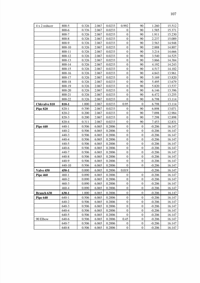
7/29/2019 Simulation and Validation of Two-component Flow in a Void Recircu
http://slidepdf.com/reader/full/simulation-and-validation-of-two-component-flow-in-a-void-recircu 123/171
107
4 x 2 reducer 800-5 0.326 2.067 0.0233 0.992 90 1.260 15.512
800-6 0.326 2.067 0.0233 0 90 1.585 15.371
800-7 0.326 2.067 0.0233 0 90 1.911 15.230
800-8 0.326 2.067 0.0233 0 90 2.237 15.089
800-9 0.326 2.067 0.0233 0 90 2.563 14.948
800-10 0.326 2.067 0.0233 0 90 2.888 14.807
800-11 0.326 2.067 0.0233 0 90 3.214 14.666
800-12 0.326 2.067 0.0233 0 90 3.540 14.525
800-13 0.326 2.067 0.0233 0 90 3.866 14.384
800-14 0.326 2.067 0.0233 0 90 4.192 14.243
800-15 0.326 2.067 0.0233 0 90 4.517 14.102
800-16 0.326 2.067 0.0233 0 90 4.843 13.961
800-17 0.326 2.067 0.0233 0 90 5.169 13.820
800-18 0.326 2.067 0.0233 0 90 5.495 13.679
800-19 0.326 2.067 0.0233 0 90 5.820 13.537
800-20 0.326 2.067 0.0233 0 90 6.146 13.396
800-21 0.326 2.067 0.0233 0 90 6.472 13.255
800-22 0.326 2.067 0.0233 0 90 6.798 13.114
Chkvalve 810 810-1 1.000 2.067 0.0233 0.95 0 6.798 13.114
Pipe 820 820-1 0.200 2.067 0.0233 0 90 6.898 13.071
820-2 0.200 2.067 0.0233 0 90 7.098 12.984
820-3 0.200 2.067 0.0233 0 90 7.298 12.898
820-4 0.311 2.067 0.0233 0 90 7.453 12.831
Pipe 440 440-1 0.506 6.065 0.2006 0 0 -0.206 16.147
440-2 0.506 6.065 0.2006 0 0 -0.206 16.147
440-3 0.506 6.065 0.2006 0 0 -0.206 16.147
440-4 0.506 6.065 0.2006 0 0 -0.206 16.147
440-5 0.506 6.065 0.2006 0 0 -0.206 16.147
440-6 0.506 6.065 0.2006 0 0 -0.206 16.147440-7 0.506 6.065 0.2006 0 0 -0.206 16.147
440-8 0.506 6.065 0.2006 0 0 -0.206 16.147
440-9 0.506 6.065 0.2006 0 0 -0.206 16.147
440-10 0.506 6.065 0.2006 0 0 -0.206 16.147
Valve 450 450-1 0.000 6.065 0.2006 0.019 -0.206 16.147
Pipe 460 460-1 0.890 6.065 0.2006 0 0 -0.206 16.147
460-2 0.890 6.065 0.2006 0 0 -0.206 16.147
460-3 0.890 6.065 0.2006 0 0 -0.206 16.147
460-4 0.890 6.065 0.2006 0 0 -0.206 16.147
Branch 630 630-1 1.000 6.065 0.2006 0 0 -0.206 16.147
Pipe 640 640-1 0.506 6.065 0.2006 0 0 -0.206 16.147640-2 0.506 6.065 0.2006 0 0 -0.206 16.147
640-3 0.506 6.065 0.2006 0 0 -0.206 16.147
640-4 0.506 6.065 0.2006 0 0 -0.206 16.147
640-5 0.506 6.065 0.2006 0 0 -0.206 16.147
90 Elbow 640-6 0.506 6.065 0.2006 0.45 0 -0.206 16.147
640-7 0.506 6.065 0.2006 0 0 -0.206 16.147
640-8 0.506 6.065 0.2006 0 0 -0.206 16.147
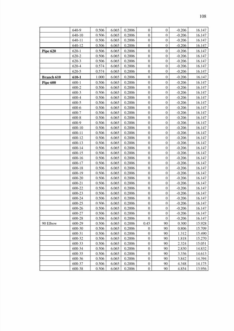
7/29/2019 Simulation and Validation of Two-component Flow in a Void Recircu
http://slidepdf.com/reader/full/simulation-and-validation-of-two-component-flow-in-a-void-recircu 124/171
108
640-9 0.506 6.065 0.2006 0 0 -0.206 16.147
640-10 0.506 6.065 0.2006 0 0 -0.206 16.147
640-11 0.506 6.065 0.2006 0 0 -0.206 16.147
640-12 0.506 6.065 0.2006 0 0 -0.206 16.147
Pipe 620 620-1 0.506 6.065 0.2006 0 0 -0.206 16.147
620-2 0.506 6.065 0.2006 0 0 -0.206 16.147620-3 0.506 6.065 0.2006 0 0 -0.206 16.147
620-4 0.574 6.065 0.2006 0 0 -0.206 16.147
620-5 0.574 6.065 0.2006 0 0 -0.206 16.147
Branch 610 610-1 1.000 6.065 0.2006 0 0 -0.206 16.147
Pipe 600 600-1 0.506 6.065 0.2006 0 0 -0.206 16.147
600-2 0.506 6.065 0.2006 0 0 -0.206 16.147
600-3 0.506 6.065 0.2006 0 0 -0.206 16.147
600-4 0.506 6.065 0.2006 0 0 -0.206 16.147
600-5 0.506 6.065 0.2006 0 0 -0.206 16.147
600-6 0.506 6.065 0.2006 0 0 -0.206 16.147
600-7 0.506 6.065 0.2006 0 0 -0.206 16.147
600-8 0.506 6.065 0.2006 0 0 -0.206 16.147
600-9 0.506 6.065 0.2006 0 0 -0.206 16.147
600-10 0.506 6.065 0.2006 0 0 -0.206 16.147
600-11 0.506 6.065 0.2006 0 0 -0.206 16.147
600-12 0.506 6.065 0.2006 0 0 -0.206 16.147
600-13 0.506 6.065 0.2006 0 0 -0.206 16.147
600-14 0.506 6.065 0.2006 0 0 -0.206 16.147
600-15 0.506 6.065 0.2006 0 0 -0.206 16.147
600-16 0.506 6.065 0.2006 0 0 -0.206 16.147
600-17 0.506 6.065 0.2006 0 0 -0.206 16.147
600-18 0.506 6.065 0.2006 0 0 -0.206 16.147
600-19 0.506 6.065 0.2006 0 0 -0.206 16.147600-20 0.506 6.065 0.2006 0 0 -0.206 16.147
600-21 0.506 6.065 0.2006 0 0 -0.206 16.147
600-22 0.506 6.065 0.2006 0 0 -0.206 16.147
600-23 0.506 6.065 0.2006 0 0 -0.206 16.147
600-24 0.506 6.065 0.2006 0 0 -0.206 16.147
600-25 0.506 6.065 0.2006 0 0 -0.206 16.147
600-26 0.506 6.065 0.2006 0 0 -0.206 16.147
600-27 0.506 6.065 0.2006 0 0 -0.206 16.147
600-28 0.506 6.065 0.2006 0 0 -0.206 16.147
90 Elbow 600-29 0.506 6.065 0.2006 0.45 90 0.300 15.928
600-30 0.506 6.065 0.2006 0 90 0.806 15.709
600-31 0.506 6.065 0.2006 0 90 1.312 15.490
600-32 0.506 6.065 0.2006 0 90 1.818 15.270
600-33 0.506 6.065 0.2006 0 90 2.324 15.051
600-34 0.506 6.065 0.2006 0 90 2.830 14.832
600-35 0.506 6.065 0.2006 0 90 3.336 14.613
600-36 0.506 6.065 0.2006 0 90 3.842 14.394
600-37 0.506 6.065 0.2006 0 90 4.348 14.175
600-38 0.506 6.065 0.2006 0 90 4.854 13.956
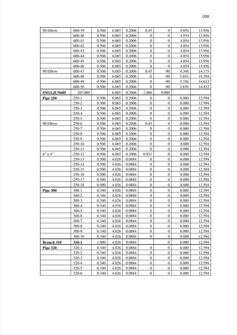
7/29/2019 Simulation and Validation of Two-component Flow in a Void Recircu
http://slidepdf.com/reader/full/simulation-and-validation-of-two-component-flow-in-a-void-recircu 125/171
109
90 Elbow 600-39 0.506 6.065 0.2006 0.45 0 4.854 13.956
600-40 0.506 6.065 0.2006 0 0 4.854 13.956
600-41 0.506 6.065 0.2006 0 0 4.854 13.956
600-42 0.506 6.065 0.2006 0 0 4.854 13.956
600-43 0.506 6.065 0.2006 0 0 4.854 13.956
600-44 0.506 6.065 0.2006 0 0 4.854 13.956
600-45 0.506 6.065 0.2006 0 0 4.854 13.956
600-46 0.506 6.065 0.2006 0 0 4.854 13.956
90 Elbow 600-47 0.506 6.065 0.2006 0.45 -90 4.348 14.175
600-48 0.506 6.065 0.2006 0 -90 3.842 14.394
600-49 0.506 6.065 0.2006 0 -90 3.336 14.613
600-50 0.506 6.065 0.2006 0 -90 2.830 14.832
SNGLJUN605 105.000 6.065 0.2006 1.000 0.000
Pipe 250 250-1 0.506 6.065 0.2006 0 0 8.000 12.594
250-2 0.506 6.065 0.2006 0 0 8.000 12.594
250-3 0.506 6.065 0.2006 0 0 8.000 12.594
250-4 0.506 6.065 0.2006 0 0 8.000 12.594
250-5 0.506 6.065 0.2006 0 0 8.000 12.594
90 Elbow 250-6 0.506 6.065 0.2006 0.45 0 8.000 12.594
250-7 0.506 6.065 0.2006 0 0 8.000 12.594
250-8 0.506 6.065 0.2006 0 0 8.000 12.594
250-9 0.506 6.065 0.2006 0 0 8.000 12.594
250-10 0.506 6.065 0.2006 0 0 8.000 12.594
250-11 0.506 6.065 0.2006 0 0 8.000 12.594
6" x 4" 250-12 0.506 6.065 0.2006 0.931 0 8.000 12.594
250-13 0.500 4.026 0.0884 0 0 8.000 12.594
250-14 0.500 4.026 0.0884 0 0 8.000 12.594
250-15 0.500 4.026 0.0884 0 0 8.000 12.594
250-16 0.500 4.026 0.0884 0 0 8.000 12.594250-17 0.500 4.026 0.0884 0 0 8.000 12.594
250-18 0.500 4.026 0.0884 0 0 8.000 12.594
Pipe 300 300-1 0.340 4.026 0.0884 0 0 8.000 12.594
300-2 0.340 4.026 0.0884 0 0 8.000 12.594
300-3 0.340 4.026 0.0884 0 0 8.000 12.594
300-4 0.340 4.026 0.0884 0 0 8.000 12.594
300-5 0.340 4.026 0.0884 0 0 8.000 12.594
300-6 0.340 4.026 0.0884 0 0 8.000 12.594
300-7 0.340 4.026 0.0884 0 0 8.000 12.594
300-8 0.340 4.026 0.0884 0 0 8.000 12.594
300-9 0.340 4.026 0.0884 0 0 8.000 12.594
300-10 0.340 4.026 0.0884 0 0 8.000 12.594
Branch 310 310-1 1.000 4.026 0.0884 0 8.000 12.594
Pipe 320 320-1 0.340 4.026 0.0884 0 0 8.000 12.594
320-2 0.340 4.026 0.0884 0 0 8.000 12.594
320-3 0.340 4.026 0.0884 0 0 8.000 12.594
320-4 0.340 4.026 0.0884 0 0 8.000 12.594
320-5 0.340 4.026 0.0884 0 0 8.000 12.594
320-6 0.340 4.026 0.0884 0 0 8.000 12.594

7/29/2019 Simulation and Validation of Two-component Flow in a Void Recircu
http://slidepdf.com/reader/full/simulation-and-validation-of-two-component-flow-in-a-void-recircu 126/171

7/29/2019 Simulation and Validation of Two-component Flow in a Void Recircu
http://slidepdf.com/reader/full/simulation-and-validation-of-two-component-flow-in-a-void-recircu 127/171
111
700-22 0.263 2.067 0.0233 0 90 6.978 13.036
Chkvalve 710 710-1 1.000 2.067 0.0233 0.95 0 6.978 13.036
Pipe 720 720-1 0.200 2.067 0.0233 0 90 7.078 12.993
720-2 0.200 2.067 0.0233 0 90 7.278 12.906
720-3 0.200 2.067 0.0233 0 90 7.478 12.820
720-4 0.311 2.067 0.0233 0 90 7.634 12.752Pipe 340 340-1 0.350 4.026 0.0884 0 0 1.348 15.474
340-2 0.350 4.026 0.0884 0 0 1.348 15.474
340-3 0.350 4.026 0.0884 0 0 1.348 15.474
340-4 0.350 4.026 0.0884 0 0 1.348 15.474
340-5 0.350 4.026 0.0884 0 0 1.348 15.474
340-6 0.350 4.026 0.0884 0 0 1.348 15.474
340-7 0.350 4.026 0.0884 0 0 1.348 15.474
340-8 0.350 4.026 0.0884 0 0 1.348 15.474
340-9 0.350 4.026 0.0884 0 0 1.348 15.474
340-10 0.350 4.026 0.0884 0 0 1.348 15.474
340-11 0.350 4.026 0.0884 0 0 1.348 15.474
340-12 0.350 4.026 0.0884 0 0 1.348 15.474
340-13 0.350 4.026 0.0884 0 0 1.348 15.474
340-14 0.350 4.026 0.0884 0 0 1.348 15.474
Valve 350 350-1 0.000 4.026 0.0884 0.019 1.348 15.474
Pipe 360 360-1 0.506 4.026 0.0884 0 0 0.000 16.147
360-2 0.506 4.026 0.0884 0 0 0.000 16.147
360-3 0.506 4.026 0.0884 0 0 0.000 16.147
6" x 4" 360-4 0.506 4.026 0.0884 0.931 0 0.000 16.147
360-5 0.900 6.065 0.2006 0 0 0.000 16.147
360-6 0.900 6.065 0.2006 0 0 0.000 16.147
360-7 0.900 6.065 0.2006 0 0.000 16.147

7/29/2019 Simulation and Validation of Two-component Flow in a Void Recircu
http://slidepdf.com/reader/full/simulation-and-validation-of-two-component-flow-in-a-void-recircu 128/171
112
Appendix C – VRS RELAP5 Code
=vrs_443_1
* This case evaluates transient two-phase flow in the 4 inch test loop
*
* Fr = 0.80, 4x4x3 Pipe configuration, Initial Void Fraction ~ 8%*
*
*cardno Problem Type Problem Option0000100 new transnt
*
*----------------------------------------------------------------------
**cardno
0000101 run
*
*----------------------------------------------------------------------*
*cardno Input Units Output Units0000102 british british
*
*cardno NonCondensable Gas Type
0000110 air*
*----------------------------------------------------------------------
*Time Step Control Cards*
*cardno time end min time step max time step ssdtt min major rstrt
0000201 5.0 1.0e-6 0.01 0003 100 1000 100000000
0000202 10.0 1.0e-6 1.0e-2 0003 100 1000 1000000000000203 20.0 1.0e-6 1.0e-2 0003 100 1000 100000000
0000204 30.0 1.0e-6 1.0e-3 0003 1000 10000 100000000
0000205 40.0 1.0e-6 1.0e-3 0003 1000 10000 1000000000000206 60.0 1.0e-6 1.0e-3 0003 1000 10000 100000000
0000207 150.0 1.0e-6 1.0e-3 0003 1000 10000 100000000
*
*----------------------------------------------------------------------*
*Minor Edit Variables
**cardno Variable Code Parameter
0000301 dt 0
0000302 cputime 0
0000303 dtcrnt 00000304 emass 0
0000305 p 300050000
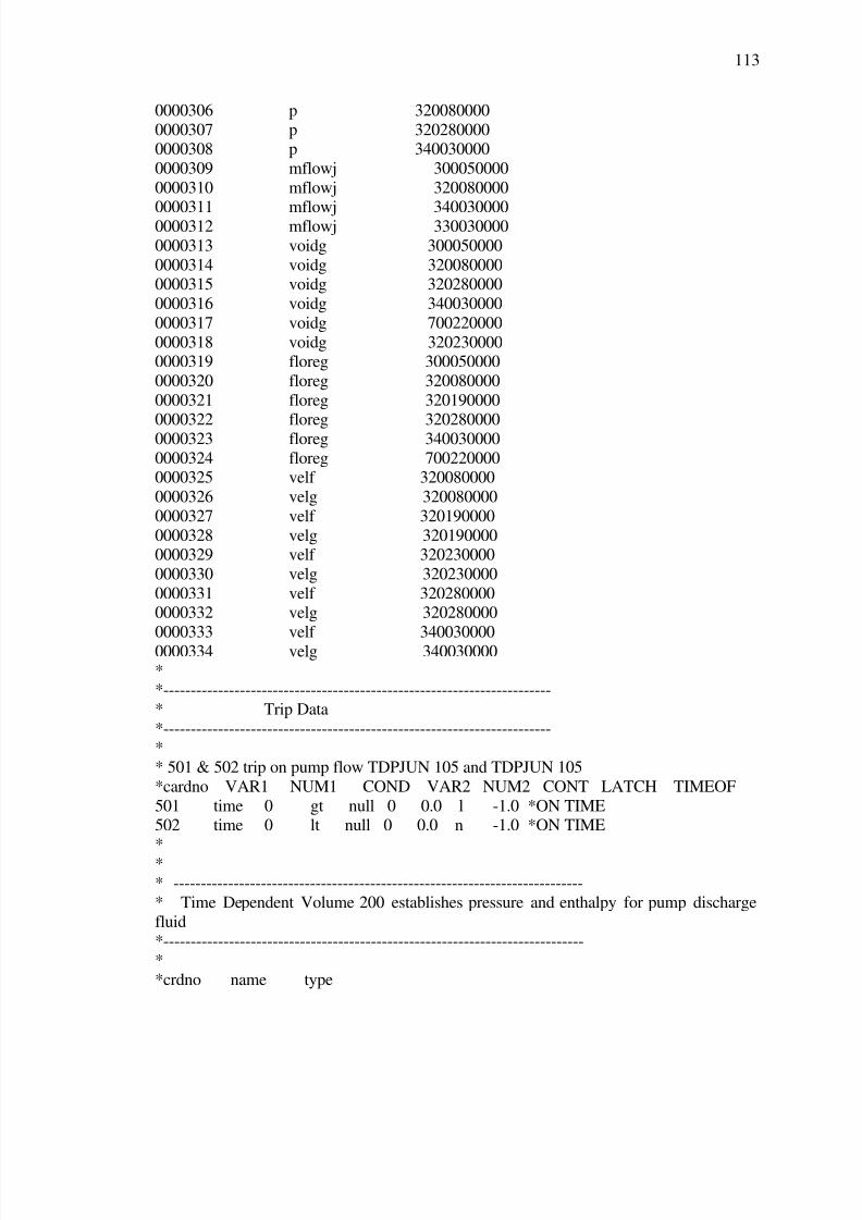
7/29/2019 Simulation and Validation of Two-component Flow in a Void Recircu
http://slidepdf.com/reader/full/simulation-and-validation-of-two-component-flow-in-a-void-recircu 129/171
113
0000306 p 320080000
0000307 p 3202800000000308 p 340030000
0000309 mflowj 300050000
0000310 mflowj 320080000
0000311 mflowj 3400300000000312 mflowj 330030000
0000313 voidg 300050000
0000314 voidg 3200800000000315 voidg 320280000
0000316 voidg 340030000
0000317 voidg 700220000
0000318 voidg 3202300000000319 floreg 300050000
0000320 floreg 320080000
0000321 floreg 320190000
0000322 floreg 3202800000000323 floreg 340030000
0000324 floreg 7002200000000325 velf 320080000
0000326 velg 320080000
0000327 velf 320190000
0000328 velg 3201900000000329 velf 320230000
0000330 velg 320230000
0000331 velf 3202800000000332 velg 320280000
0000333 velf 340030000
0000334 velg 340030000
**-----------------------------------------------------------------------
* Trip Data
*-----------------------------------------------------------------------*
* 501 & 502 trip on pump flow TDPJUN 105 and TDPJUN 105
*cardno VAR1 NUM1 COND VAR2 NUM2 CONT LATCH TIMEOF
501 time 0 gt null 0 0.0 l -1.0 *ON TIME502 time 0 lt null 0 0.0 n -1.0 *ON TIME
*
** ---------------------------------------------------------------------------
* Time Dependent Volume 200 establishes pressure and enthalpy for pump discharge
fluid
*-----------------------------------------------------------------------------*
*crdno name type
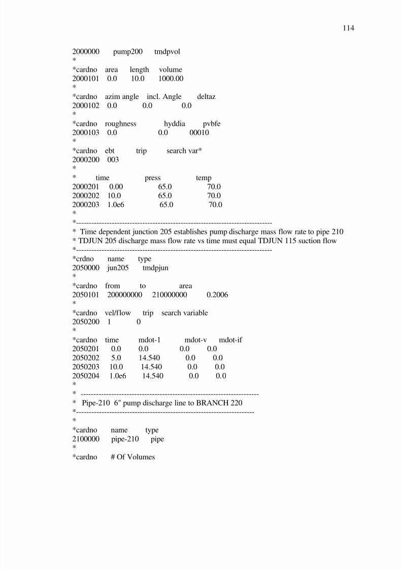
7/29/2019 Simulation and Validation of Two-component Flow in a Void Recircu
http://slidepdf.com/reader/full/simulation-and-validation-of-two-component-flow-in-a-void-recircu 130/171
114
2000000 pump200 tmdpvol
**cardno area length volume
2000101 0.0 10.0 1000.00
*
*cardno azim angle incl. Angle deltaz2000102 0.0 0.0 0.0
*
*cardno roughness hyddia pvbfe2000103 0.0 0.0 00010
*
*cardno ebt trip search var*
2000200 003*
* time press temp
2000201 0.00 65.0 70.0
2000202 10.0 65.0 70.02000203 1.0e6 65.0 70.0
**-----------------------------------------------------------------------------
* Time dependent junction 205 establishes pump discharge mass flow rate to pipe 210
* TDJUN 205 discharge mass flow rate vs time must equal TDJUN 115 suction flow
*-----------------------------------------------------------------------------*crdno name type
2050000 jun205 tmdpjun
**cardno from to area
2050101 200000000 210000000 0.2006
*
*cardno vel/flow trip search variable2050200 1 0
*
*cardno time mdot-1 mdot-v mdot-if 2050201 0.0 0.0 0.0 0.0
2050202 5.0 14.540 0.0 0.0
2050203 10.0 14.540 0.0 0.0
2050204 1.0e6 14.540 0.0 0.0*
* ----------------------------------------------------------------------
* Pipe-210 6" pump discharge line to BRANCH 220*----------------------------------------------------------------------
*
*cardno name type
2100000 pipe-210 pipe*
*cardno # Of Volumes
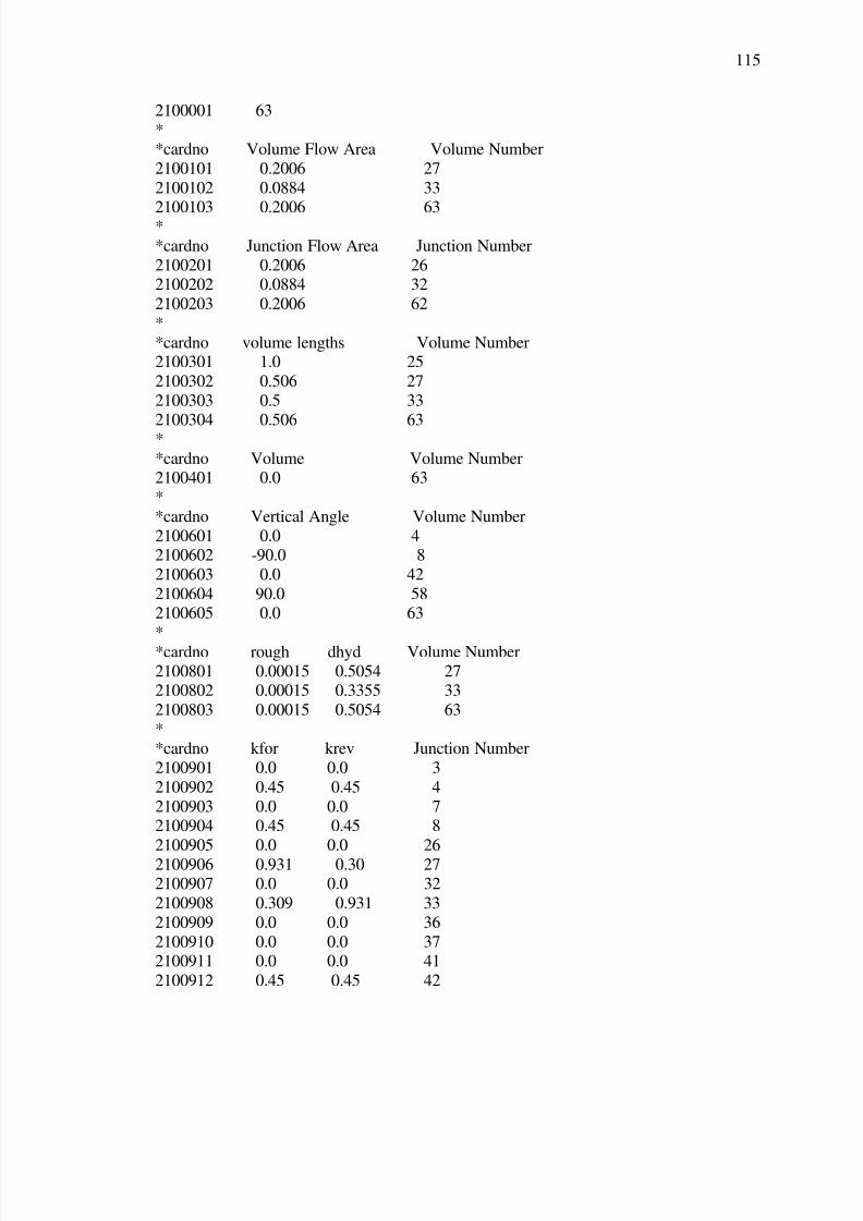
7/29/2019 Simulation and Validation of Two-component Flow in a Void Recircu
http://slidepdf.com/reader/full/simulation-and-validation-of-two-component-flow-in-a-void-recircu 131/171
115
2100001 63
**cardno Volume Flow Area Volume Number
2100101 0.2006 27
2100102 0.0884 33
2100103 0.2006 63*
*cardno Junction Flow Area Junction Number
2100201 0.2006 262100202 0.0884 32
2100203 0.2006 62
*
*cardno volume lengths Volume Number2100301 1.0 25
2100302 0.506 27
2100303 0.5 33
2100304 0.506 63*
*cardno Volume Volume Number2100401 0.0 63
*
*cardno Vertical Angle Volume Number
2100601 0.0 42100602 -90.0 8
2100603 0.0 42
2100604 90.0 582100605 0.0 63
*
*cardno rough dhyd Volume Number
2100801 0.00015 0.5054 272100802 0.00015 0.3355 33
2100803 0.00015 0.5054 63
**cardno kfor krev Junction Number
2100901 0.0 0.0 3
2100902 0.45 0.45 4
2100903 0.0 0.0 72100904 0.45 0.45 8
2100905 0.0 0.0 26
2100906 0.931 0.30 272100907 0.0 0.0 32
2100908 0.309 0.931 33
2100909 0.0 0.0 36
2100910 0.0 0.0 372100911 0.0 0.0 41
2100912 0.45 0.45 42

7/29/2019 Simulation and Validation of Two-component Flow in a Void Recircu
http://slidepdf.com/reader/full/simulation-and-validation-of-two-component-flow-in-a-void-recircu 132/171
116
2100913 0.0 0.0 57
2100914 0.45 0.45 582100915 0.0 0.0 62
*
*cardno tlpvbfe Volume Number
2101001 0010000 63*
*cardno efvchas Junction Number
2101101 0001000 62*
*cardno ic press temp qual vol.
2101201 3 14.584 70.0 0.0 0.0 0.0 4
2101202 3 14.800 70.0 0.0 0.0 0.0 52101203 3 15.233 70.0 0.0 0.0 0.0 6
2101204 3 15.666 70.0 0.0 0.0 0.0 7
2101205 3 16.099 70.0 0.0 0.0 0.0 42
2101206 3 15.880 70.0 0.0 0.0 0.0 432101207 3 15.661 70.0 0.0 0.0 0.0 44
2101208 3 15.442 70.0 0.0 0.0 0.0 452101209 3 15.223 70.0 0.0 0.0 0.0 46
2101210 3 15.004 70.0 0.0 0.0 0.0 47
2101211 3 14.785 70.0 0.0 0.0 0.0 48
2101212 3 14.565 70.0 0.0 0.0 0.0 492101213 3 14.346 70.0 0.0 0.0 0.0 50
2101214 3 14.127 70.0 0.0 0.0 0.0 51
2101215 3 14.908 70.0 0.0 0.0 0.0 522101216 3 13.689 70.0 0.0 0.0 0.0 53
2101217 3 13.470 70.0 0.0 0.0 0.0 54
2101218 3 13.251 70.0 0.0 0.0 0.0 55
2101219 3 13.032 70.0 0.0 0.0 0.0 562101220 3 12.813 70.0 0.0 0.0 0.0 57
2101221 3 12.594 70.0 0.0 0.0 0.0 63
**cardno vel/flow
2101300 1
*
*cardno liqflow vaporf interv jun2101301 0.0 0.0 0.0 62
*
*cardno jct dh beta c m jun2101401 0.0 0.0 1.0 1.0 62
*
*
*----------------------------------------------------------------------* Branch 220 6"x6"x6" branch tee connecting pipe-210, pipe-500, and pipe-230
*----------------------------------------------------------------------

7/29/2019 Simulation and Validation of Two-component Flow in a Void Recircu
http://slidepdf.com/reader/full/simulation-and-validation-of-two-component-flow-in-a-void-recircu 133/171
117
*
*cardno name type2200000 brnch220 branch
*
*cardno number junctions initial condition control
2200001 3 1*
*cardno v.flowarea vlength v. h-ang v-ang delz rough dhy tlpvbfe
2200101 0.2006 1.0 0.0 0.0 0.0 0.0 0.00015 0.5054 0010000*
*cardno ctl pressure temp qual
2200200 003 12.594 70.0
** K thru = 20 ft = 20 x .015 = 0.3
* K branch floss = 60 ft = 60 x .015 = 0.9
*cardno from to area floss rloss efvcahs
2201101 210010000 220000000 0.2006 0.00 0.00 00011002202101 220010000 500000000 0.2006 0.30 0.30 0001100
2203101 220010000 230000000 0.2006 0.90 0.90 0001100*
*
*cardno flowf flowg velj
2201201 0.0 0.0 0.02202201 0.0 0.0 0.0
2203201 0.0 0.0 0.0
**----------------------------------------------------------------------
* Pipe-230 6" line - 6" branch 220 to branch 240
*----------------------------------------------------------------------
**cardno name type
2300000 pipe-230 pipe
**cardno # Of Volumes
2300001 5
*
*cardno Volume Flow Area Volume Number2300101 0.2006 5
*
*cardno Junction Flow Area Junction Number2300201 0.2006 4
*
*cardno volume lengths Volume Number
2300301 0.506 42300302 0.643 5
*
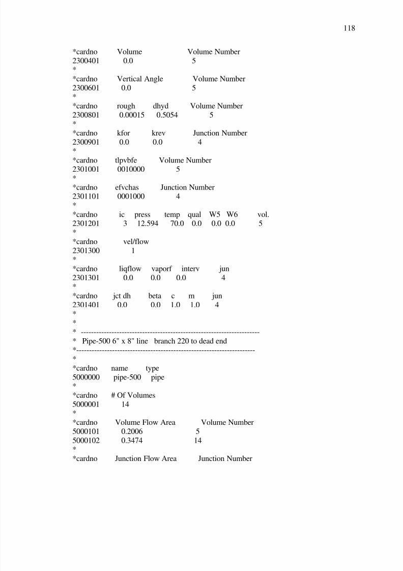
7/29/2019 Simulation and Validation of Two-component Flow in a Void Recircu
http://slidepdf.com/reader/full/simulation-and-validation-of-two-component-flow-in-a-void-recircu 134/171
118
*cardno Volume Volume Number
2300401 0.0 5*
*cardno Vertical Angle Volume Number
2300601 0.0 5
**cardno rough dhyd Volume Number
2300801 0.00015 0.5054 5
**cardno kfor krev Junction Number
2300901 0.0 0.0 4
*
*cardno tlpvbfe Volume Number2301001 0010000 5
*
*cardno efvchas Junction Number
2301101 0001000 4*
*cardno ic press temp qual W5 W6 vol.2301201 3 12.594 70.0 0.0 0.0 0.0 5
*
*cardno vel/flow
2301300 1*
*cardno liqflow vaporf interv jun
2301301 0.0 0.0 0.0 4*
*cardno jct dh beta c m jun
2301401 0.0 0.0 1.0 1.0 4
**
* ----------------------------------------------------------------------
* Pipe-500 6" x 8" line branch 220 to dead end*----------------------------------------------------------------------
*
*cardno name type
5000000 pipe-500 pipe*
*cardno # Of Volumes
5000001 14*
*cardno Volume Flow Area Volume Number
5000101 0.2006 5
5000102 0.3474 14*
*cardno Junction Flow Area Junction Number
7/29/2019 Simulation and Validation of Two-component Flow in a Void Recircu
http://slidepdf.com/reader/full/simulation-and-validation-of-two-component-flow-in-a-void-recircu 135/171
119
5000201 0.2006 4
5000202 0.3474 13*
*cardno volume lengths Volume Number
5000301 0.506 5
5000302 0.700 135000303 0.900 14
*
*cardno Volume Volume Number5000401 0.0 14
*
*
*cardno Vertical Angle Volume Number5000601 0.0 14
*
*cardno rough dhyd Volume Number
5000801 0.00015 0.5054 55000802 0.00015 0.6651 14
**cardno kfor krev Junction Number
5000901 0.0 0.0 4
5000902 0.191 0.472 5
5000903 0.0 0.0 13*
*cardno tlpvbfe Volume Number
5001001 0010000 14*
*cardno efvchas Junction Number
5001101 0001000 13
**cardno ic press temp qual W5 W6 vol.
5001201 3 12.594 70.0 0.0 0.0 0.0 14
**cardno vel/flow
5001300 1
*
*cardno liqflow vaporf interv jun5001301 0.0 0.0 0.0 13
*
*cardno jct dh beta c m jun5001401 0.0 0.0 1.0 1.0 13
*
*
*----------------------------------------------------------------------* Branch 240 6"x6"x6" branch tee connecting pipe-230, pipe-250, and pipe-400
*----------------------------------------------------------------------

7/29/2019 Simulation and Validation of Two-component Flow in a Void Recircu
http://slidepdf.com/reader/full/simulation-and-validation-of-two-component-flow-in-a-void-recircu 136/171
120
*
*cardno name type2400000 brnch240 branch
*
*cardno number junctions initial condition control
2400001 3 1*
*cardno v.flowarea vlength v. h-ang v-ang delz rough dhy tlpvbfe
2400101 0.2006 1.0 0.0 0.0 0.0 0.0 0.00015 0.5054 0010000*
*cardno ctl pressure temp qual
2400200 003 12.594 70.0
** K thru = 20 ft = 20 x .015 = 0.3
* K branch floss = 60 ft = 60 x .015 = 0.9
*cardno from to area floss rloss efvcahs
2401101 230010000 240000000 0.2006 0.00 0.00 00011002402101 240010000 250000000 0.2006 0.30 0.30 0001100
2403101 240010000 400000000 0.2006 0.90 0.90 0001100*
*cardno flowf flowg velj
2401201 0.0 0.0 0.0
2402201 0.0 0.0 0.02403201 0.0 0.0 0.0
*
* ----------------------------------------------------------------------* Pipe-400 6" test loop line connecting Branch 240 - Dead end
*----------------------------------------------------------------------
*
*cardno name type4000000 pipe-400 pipe
*
*cardno # Of Volumes4000001 9
*
*cardno Volume Flow Area Volume Number
4000101 0.2006 9*
*cardno Junction Flow Area Junction Number
4000201 0.2006 8*
*cardno volume lengths Volume Number
4000301 0.506 8
4000302 0.535 9*
*cardno Volume Volume Number

7/29/2019 Simulation and Validation of Two-component Flow in a Void Recircu
http://slidepdf.com/reader/full/simulation-and-validation-of-two-component-flow-in-a-void-recircu 137/171
121
4000401 0.0 9
**cardno Vertical Angle Volume Number
4000601 0.0 9
*
*cardno rough dhyd Volume Number
4000801 0.00015 0.5054 9
**cardno kfor krev Junction Number
4000901 0.0 0.0 8
*
*cardno tlpvbfe Volume Number4001001 0010000 9
*
*cardno efvchas Junction Number
4001101 0001000 8*
*cardno ic press temp qual W5 W6 vol.4001201 3 12.594 70.0 0.0 0.0 0.0 9
*
*cardno vel/flow
4001300 1*
*cardno liqflow vaporf interv jun
4001301 0.0 0.0 0.0 8*
*cardno jct dh beta c m jun
4001401 0.0 0.0 1.0 1.0 8
**
* ----------------------------------------------------------------------
* Pipe-300 4" test loop line connecting Branch 407 to Branch 310*----------------------------------------------------------------------
*
*cardno name type
3000000 pipe-300 pipe*
*cardno # Of Volumes
3000001 10*
*cardno Volume Flow Area Volume Number
3000101 0.0884 10
**cardno Junction Flow Area Junction Number
3000201 0.0884 9
7/29/2019 Simulation and Validation of Two-component Flow in a Void Recircu
http://slidepdf.com/reader/full/simulation-and-validation-of-two-component-flow-in-a-void-recircu 138/171
122
*
*cardno volume lengths Volume Number3000301 0.340 10
*
*cardno Volume Volume Number
3000401 0.0 10*
*cardno Vertical Angle Volume Number
3000601 0.0 10*
*cardno rough dhyd Volume Number
3000801 0.00015 0.3355 10*
*cardno kfor krev Junction Number
3000901 0.0 0.0 9
**cardno tlpvbfe Volume Number
3001001 0010000 10*
*cardno efvchas Junction Number
3001101 0001000 9
**cardno ic press temp qual W5 W6 vol.
3001201 3 12.594 70.0 0.0 0.0 0.0 10
**cardno vel/flow
3001300 1
*
*cardno liqflow vaporf interv jun3001301 0.0 0.0 0.0 9
**cardno jct dh beta c m jun
3001401 0.0 0.0 1.0 1.0 9
*
** ---------------------------------------------------------------------------
* Time Dependent Volume 402 establishes pressure for air discharge
*-----------------------------------------------------------------------------*
*crdno name type
4020000 rsrvr402 tmdpvol
**cardno area length volume
4020101 10.0 1.0e6 0.0

7/29/2019 Simulation and Validation of Two-component Flow in a Void Recircu
http://slidepdf.com/reader/full/simulation-and-validation-of-two-component-flow-in-a-void-recircu 139/171
123
*
*cardno azim angle incl. Angle deltaz4020102 0.0 0.0 0.0
*
*cardno roughness hyddia pvbfe
4020103 0.000005 0.0 00010*
*cardno ebt trip search var*
4020200 004*
* time press temp equil-quality
4020201 0.00 120.0 70.0 0
4020202 5.00 120.0 70.0 04020203 10.00 120.0 70.0 0
4020204 20.00 120.0 70.0 0
4020205 1.0e6 120.0 70.0 0
**
*-----------------------------------------------------------------------------* Time dependent junction 403 establishes air compressor discharge flowrate to
SNGLVOL 404
*-----------------------------------------------------------------------------
**cardno name type
4030000 comp403 tmdpjun
**cardno from to Junction Area (ft2)
4030101 402010000 404000000 0.00072
*
*cardno vel/flow trip search variable4030200 1 0
*
*cardno time v-l v-g v-if 4030201 0.00 0.0 0.0 0.0
4030202 5.00 0.0 0.0 0.0
4030203 17.00 0.0 0.0 0.0
4030204 18.00 0.0 0.5e-3 0.04030205 19.00 0.0 1.0e-3 0.0
4030206 20.00 0.0 3.0e-3 0.0
4030207 35.00 0.0 3.0e-3 0.04030208 36.00 0.0 2.8e-3 0.0
4030209 37.00 0.0 2.6e-3 0.0
4030210 38.00 0.0 2.4e-3 0.0
4030211 39.00 0.0 2.0e-3 0.04030212 40.00 0.0 1.6e-3 0.0
4030213 41.00 0.0 1.2e-3 0.0

7/29/2019 Simulation and Validation of Two-component Flow in a Void Recircu
http://slidepdf.com/reader/full/simulation-and-validation-of-two-component-flow-in-a-void-recircu 140/171
124
4030214 42.00 0.0 0.0 0.0
4030215 1.0e6 0.0 0.0 0.0*
*
*----------------------------------------------------------------------
* Single Volume, Component 404 1/2" Pipe*----------------------------------------------------------------------
*
*crdno name type4040000 pipe404 snglvol
*
*cardno area length volume
4040101 0.00072 2.0 0.0*
*cardno azim angle incl. Angle deltaz
4040102 0 0.0 0.0
**cardno roughness hyddia tlpvbfe
4040103 0.000005 0.03033 0001000*
*cardno ebt pressure temperature equil-quality
4040200 003 12.594 70.0
**
*----------------------------------------------------------------------
* Checkvalve 405 2" void recirc line Check Valve SNGLVOL-404 to SNGLVOL-406*----------------------------------------------------------------------
*
* NAME TYPE
4050000 chkv405 valve*
* FROM TO AREA FLC RLC JUNC FLAGS
4050101 404010000 406000000 0.00072 0.0 20.0 000100*
* CNRL LIQ VAP INTER(MASS FLOWS)
4050201 1 0.0 0.0 0.0
*4050300 chkvlv
*
* TYPE INITPOS CLPRES LEAK4050301 0 1 3.0 0.0
*
*
*----------------------------------------------------------------------* Single Volume, Component 406 1/2" Pipe
*----------------------------------------------------------------------

7/29/2019 Simulation and Validation of Two-component Flow in a Void Recircu
http://slidepdf.com/reader/full/simulation-and-validation-of-two-component-flow-in-a-void-recircu 141/171
125
*
*crdno name type4060000 pipe406 snglvol
*
*cardno area length volume
4060101 0.00072 2.0 0.0*
*cardno azim angle incl. Angle deltaz
4060102 0 0.0 0.0*
*cardno roughness hyddia tlpvbfe
4060103 0.000005 0.03033 0001000
**cardno ebt pressure temperature equil-quality
4060200 003 12.594 70.0
*
**----------------------------------------------------------------------
* Branch 407 4"x4"x4" branch tee connecting SNGLVOL-406 (air line), PIPE-250, andPIPE-300
*----------------------------------------------------------------------
*
*cardno name type4070000 brnch407 branch
*
*cardno number junctions initial condition control4070001 3 1
*
*cardno v.flowarea vlength v. h-ang v-ang delz rough dhy tlpvbfe
4070101 0.0884 1.0 0.0 0.0 0.0 0.0 0.00015 0.3355 0010000*
*cardno ctl pressure temp qual
4070200 003 12.594 70.0*
* K thru floss = 20*f = 20 x .015 = 0.30
* K branch floss = 60*f = 60 x .015 = 0.90 - Based on water data and not air - need to
acommodate for air if needed*cardno from to area floss rloss efvcahs
4071101 250010000 407000000 0.0884 0.0 0.0 0001000
4072101 406010000 407000000 0.00072 0.9 0.9 00110004073101 407010000 300000000 0.0884 0.3 0.3 0001000
*
*
*cardno flowf flowg velj4071201 0.0 0.0 0.0
4072201 0.0 0.0 0.0
7/29/2019 Simulation and Validation of Two-component Flow in a Void Recircu
http://slidepdf.com/reader/full/simulation-and-validation-of-two-component-flow-in-a-void-recircu 142/171
126
4073201 0.0 0.0 0.0
**
*----------------------------------------------------------------------
* Branch 310 4"x4"x2" branch tee connecting pipe-300, pipe-320,
* and connected to pipe-700 via check valve 710 junction*----------------------------------------------------------------------
*
*cardno name type3100000 brnch310 branch
*
*cardno number junctions initial condition control
3100001 3 1*
*cardno v.flowarea vlength v. h-ang v-ang delz rough dhy tlpvbfe
3100101 0.0884 0.3355 0.0 0.0 0.0 0.0 0.00015 0.3355 0010000
**cardno ctl pressure temp qual
3100200 003 12.594 70.0*
* K thru = 20 ft = 20 x .015 = 0.3
* K branch (2" pipe) = 60*ft = 60 x 0.019 = 1.14
* v = 1 upward oriented junction v = 2 downward oriented junction* a = 1 abrupt area change
*cardno from to area floss rloss efvcahs
3101101 300010000 310000000 0.0884 0.0 0.0 00011203102101 310010000 320000000 0.0884 0.3 0.3 0001120
3103101 720010000 310010005 0.0233 1.14 1.14 0121100
*
*cardno flowf flowg velj3101201 0.0 0.0 0.0
3102201 0.0 0.0 0.0
3103201 0.0 0.0 0.0*
*
*----------------------------------------------------------------------
* Pipe-320 4" test loop line connecting Branch 310 to Branch 330*----------------------------------------------------------------------
*
*cardno name type3200000 pipe-320 pipe
*
*cardno # Of Volumes
3200001 32*
*cardno Volume Flow Area Volume Number

7/29/2019 Simulation and Validation of Two-component Flow in a Void Recircu
http://slidepdf.com/reader/full/simulation-and-validation-of-two-component-flow-in-a-void-recircu 143/171
127
3200101 0.0884 32
**cardno Junction Flow Area Junction Number
3200201 0.2006 31
*
*cardno volume lengths Volume Number3200301 0.340 10
3200302 0.500 11
3200303 0.657 213200304 0.500 22
3200305 0.340 32
*
*cardno Volume Volume Number3200401 0.0 32
*
*cardno Vertical Angle Volume Number
3200601 0.0 103200602 -45.0 11
3200603 -90.0 213200604 -45.0 22
3200605 0.0 32
*
*cardno rough dhyd Volume Number3200801 0.00015 0.3355 32
*
*cardno kfor krev Junction Number3200901 0.00 0.00 9
3200902 0.51 0.51 10
3200903 0.00 0.00 20
3200904 0.51 0.51 213200905 0.00 0.00 31
*
*cardno tlpvbfe Volume Number3201001 0010000 32
*
*cardno efvcahs Junction Number
3201101 0001000 203201102 0000000 31
*
*cardno ic press temp qual vol.3201201 3 12.594 70.0 0.0 0.0 0.0 10
3201202 3 12.646 70.0 0.0 0.0 0.0 11
3201203 3 12.752 70.0 0.0 0.0 0.0 12
3201204 3 13.068 70.0 0.0 0.0 0.0 133201205 3 13.384 70.0 0.0 0.0 0.0 14
3201206 3 13.700 70.0 0.0 0.0 0.0 15

7/29/2019 Simulation and Validation of Two-component Flow in a Void Recircu
http://slidepdf.com/reader/full/simulation-and-validation-of-two-component-flow-in-a-void-recircu 144/171
128
3201207 3 14.016 70.0 0.0 0.0 0.0 16
3201208 3 14.332 70.0 0.0 0.0 0.0 173201209 3 14.648 70.0 0.0 0.0 0.0 18
3201210 3 14.964 70.0 0.0 0.0 0.0 19
3201211 3 15.280 70.0 0.0 0.0 0.0 20
3201212 3 15.694 70.0 0.0 0.0 0.0 213201213 3 15.820 70.0 0.0 0.0 0.0 22
3201214 3 15.872 70.0 0.0 0.0 0.0 32
**cardno vel/flow
3201300 1
*
*cardno liqflow vaporf interv jun3201301 0.0 0.0 0.0 31
*
*cardno jct dh beta c m jun
3201401 0.0 0.0 1.0 1.0 31*
**----------------------------------------------------------------------
* Branch 330 4"x4"x3" branch tee connecting pipe-320, pipe-340, and pipe-700
*----------------------------------------------------------------------
**cardno name type
3300000 brnch330 branch
**cardno number junctions initial condition control
3300001 3 1
*
*cardno v.flowarea vlength v. h-ang v-ang delz rough dhy tlpvbfe3300101 0.0884 0.5 0.0 0.0 0.0 0.0 0.00015 0.3355 0010000
*
*cardno ctl pressure temp qual3300200 003 15.872 70.0
*
* K thru = 20 ft = 20 x .017 = 0.34
* K branch floss = 60 ft + 4 x 3 reduce = 1.02 + 0.506 = 1.526* K branch rloss = 60 ft + 3 x 4 enlarge = 1.02 + 0.191 = 1.211
* * v = 1 upward oriented junction v = 2 downward oriented junction
* a = 1 abrupt area change*cardno from to area floss rloss efvcahs
3301101 320010000 330000000 0.0884 0.0 0.0 0001120
3302101 330010000 340000000 0.0884 0.3 0.3 0001120
3303101 330010006 700000000 0.0513 1.526 1.211 0111100*
*cardno flowf flowg velj
7/29/2019 Simulation and Validation of Two-component Flow in a Void Recircu
http://slidepdf.com/reader/full/simulation-and-validation-of-two-component-flow-in-a-void-recircu 145/171
129
3301201 0.0 0.0 0.0
3302201 0.0 0.0 0.03303201 0.0 0.0 0.0
*
*
* ----------------------------------------------------------------------* Pipe-700 3" x 2" void recirc test line connecting Branch 330 to chkvlve 710
*----------------------------------------------------------------------
**cardno name type
7000000 pipe-700 pipe
*
*cardno # Of Volumes7000001 22
*
*cardno Volume Flow Area Volume Number
7000101 0.0513 67000102 0.0233 22
**cardno Junction Flow Area Junction Number
7000201 0.0513 6
7000202 0.0233 21
**cardno volume lengths Volume Number
7000301 0.260 6
7000302 0.27941 22*
*cardno Volume Volume Number
7000401 0.0 22
**cardno Vertical Angle Volume Number
7000601 90.0 22
**cardno rough dhyd Volume Number
7000801 0.00015 0.2557 6
7000802 0.00015 0.1722 22
**cardno kfor krev Junction Number
7000901 0.00 0.00 5
7000902 0.992 0.309 67000903 0.00 0.00 21
*
*cardno tlpvbfe Volume Number
7001001 0010000 22*
*cardno efvchas Junction Number
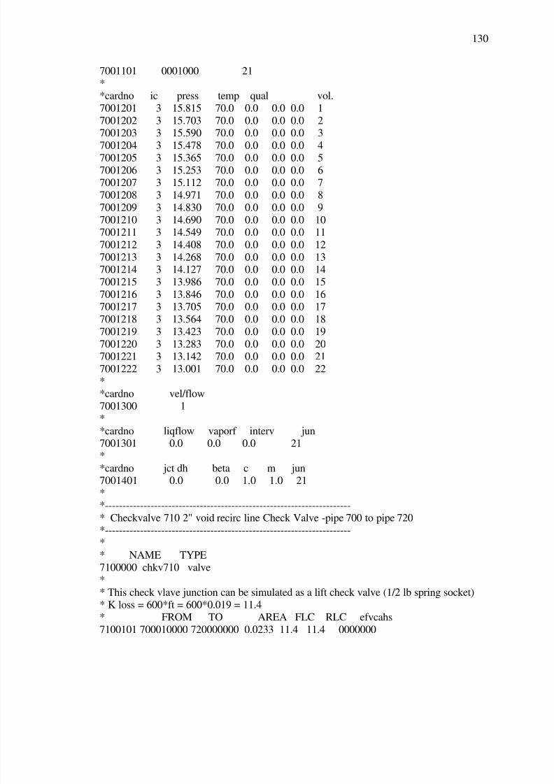
7/29/2019 Simulation and Validation of Two-component Flow in a Void Recircu
http://slidepdf.com/reader/full/simulation-and-validation-of-two-component-flow-in-a-void-recircu 146/171
130
7001101 0001000 21
**cardno ic press temp qual vol.
7001201 3 15.815 70.0 0.0 0.0 0.0 1
7001202 3 15.703 70.0 0.0 0.0 0.0 2
7001203 3 15.590 70.0 0.0 0.0 0.0 37001204 3 15.478 70.0 0.0 0.0 0.0 4
7001205 3 15.365 70.0 0.0 0.0 0.0 5
7001206 3 15.253 70.0 0.0 0.0 0.0 67001207 3 15.112 70.0 0.0 0.0 0.0 7
7001208 3 14.971 70.0 0.0 0.0 0.0 8
7001209 3 14.830 70.0 0.0 0.0 0.0 9
7001210 3 14.690 70.0 0.0 0.0 0.0 107001211 3 14.549 70.0 0.0 0.0 0.0 11
7001212 3 14.408 70.0 0.0 0.0 0.0 12
7001213 3 14.268 70.0 0.0 0.0 0.0 13
7001214 3 14.127 70.0 0.0 0.0 0.0 147001215 3 13.986 70.0 0.0 0.0 0.0 15
7001216 3 13.846 70.0 0.0 0.0 0.0 167001217 3 13.705 70.0 0.0 0.0 0.0 17
7001218 3 13.564 70.0 0.0 0.0 0.0 18
7001219 3 13.423 70.0 0.0 0.0 0.0 19
7001220 3 13.283 70.0 0.0 0.0 0.0 207001221 3 13.142 70.0 0.0 0.0 0.0 21
7001222 3 13.001 70.0 0.0 0.0 0.0 22
**cardno vel/flow
7001300 1
*
*cardno liqflow vaporf interv jun7001301 0.0 0.0 0.0 21
*
*cardno jct dh beta c m jun7001401 0.0 0.0 1.0 1.0 21
*
*----------------------------------------------------------------------
* Checkvalve 710 2" void recirc line Check Valve -pipe 700 to pipe 720*----------------------------------------------------------------------
*
* NAME TYPE7100000 chkv710 valve
*
* This check vlave junction can be simulated as a lift check valve (1/2 lb spring socket)
* K loss = 600*ft = 600*0.019 = 11.4* FROM TO AREA FLC RLC efvcahs
7100101 700010000 720000000 0.0233 11.4 11.4 0000000

7/29/2019 Simulation and Validation of Two-component Flow in a Void Recircu
http://slidepdf.com/reader/full/simulation-and-validation-of-two-component-flow-in-a-void-recircu 147/171
131
*
* CNRL LIQ VAP INTER(MASS FLOWS)7100201 1 0.0 0.0 0.0
*
7100300 chkvlv
** TYPE INITPOS CLPRES LEAK
7100301 0 1 0.596 0.0
** ----------------------------------------------------------------------
* Pipe-720 2" void recirc test line connecting CHKVLV 810 to BRANCH 410
*----------------------------------------------------------------------
**cardno name type
7200000 pipe-720 pipe
*
*cardno # Of Volumes7200001 4
**cardno Volume Flow Area Volume Number
7200101 0.0233 4
*
*cardno Junction Flow Area Junction Number7200201 0.0233 3
*
*cardno volume lengths Volume Number7200301 0.200 3
7200302 0.311 4
*
*cardno Volume Volume Number7200401 0.0 4
*
*cardno Vertical Angle Volume Number7200601 90.0 4
*
*cardno rough dhyd Volume Number
7200801 0.00015 0.1722 4*
*cardno kfor krev Junction Number
7200901 0.00 0.00 3*
*cardno tlpvbfe Volume Number
7201001 0010000 4
**cardno efvchas Junction Number
7201101 0001000 3
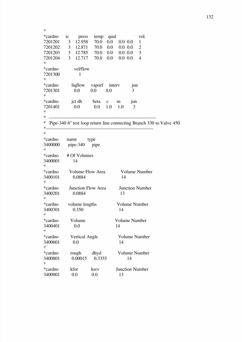
7/29/2019 Simulation and Validation of Two-component Flow in a Void Recircu
http://slidepdf.com/reader/full/simulation-and-validation-of-two-component-flow-in-a-void-recircu 148/171
132
*
*cardno ic press temp qual vol.7201201 3 12.958 70.0 0.0 0.0 0.0 1
7201202 3 12.871 70.0 0.0 0.0 0.0 2
7201203 3 12.785 70.0 0.0 0.0 0.0 3
7201204 3 12.717 70.0 0.0 0.0 0.0 4*
*cardno vel/flow
7201300 1*
*cardno liqflow vaporf interv jun
7201301 0.0 0.0 0.0 3
**cardno jct dh beta c m jun
7201401 0.0 0.0 1.0 1.0 3
*
* ----------------------------------------------------------------------* Pipe-340 6" test loop return line connecting Branch 330 to Valve 450
*----------------------------------------------------------------------*
*cardno name type
3400000 pipe-340 pipe
**cardno # Of Volumes
3400001 14
**cardno Volume Flow Area Volume Number
3400101 0.0884 14
*
*cardno Junction Flow Area Junction Number3400201 0.0884 13
*
*cardno volume lengths Volume Number3400301 0.350 14
*
*cardno Volume Volume Number
3400401 0.0 14*
*cardno Vertical Angle Volume Number
3400601 0.0 14*
*cardno rough dhyd Volume Number
3400801 0.00015 0.3355 14
**cardno kfor krev Junction Number
3400901 0.0 0.0 13

7/29/2019 Simulation and Validation of Two-component Flow in a Void Recircu
http://slidepdf.com/reader/full/simulation-and-validation-of-two-component-flow-in-a-void-recircu 149/171
133
*
*cardno tlpvbfe Volume Number3401001 0010010 14
*
*cardno efvcahs Junction Number
3401101 0001000 13*
*cardno ic press temp qual W5 W6 vol.
3401201 3 15.774 70.0 0.0 0.0 0.0 14*
*cardno vel/flow
3401300 1
**cardno liqflow vaporf interv jun
3401301 0.0 0.0 0.0 13
*
*cardno jct dh beta c m jun3401401 0.0 0.0 1.0 1.0 13
**
*----------------------------------------------------------------------
* Valve 350 - 4 " loop test line isolation valve Pipe 340 to Pipe 360
*----------------------------------------------------------------------*
* NAME TYPE
3500000 vlv450 valve*
* Crane Eqn 2-6 k = (29.9 d^2 / Cv )^2 = 0.02399
* Where Cv = 3129 gpm/psi
* FROM TO AREA FLC RLC efvcahs3500101 340010000 360000000 0.0884 0.024 0.024 0001000
*
* CNRL LIQ VAP INTER(MASS FLOWS)3500201 1 0.0 0.0 0.0
*
* TYPE
3500300 trpvlv*
* TRIP
3500301 501*
* ----------------------------------------------------------------------
* Pipe-360 6" test loop return line connecting Branch 430 to Valve 450
*----------------------------------------------------------------------*
*cardno name type

7/29/2019 Simulation and Validation of Two-component Flow in a Void Recircu
http://slidepdf.com/reader/full/simulation-and-validation-of-two-component-flow-in-a-void-recircu 150/171
134
3600000 pipe-360 pipe
**cardno # Of Volumes
3600001 7
*
*cardno Volume Flow Area Volume Number3600101 0.0884 4
3600102 0.2006 7
**cardno Junction Flow Area Junction Number
3600201 0.0884 3
3600202 0.2006 6
**cardno volume lengths Volume Number
3600301 0.506 4
3600302 0.900 7
**cardno Volume Volume Number
3600401 0.0 7*
*cardno Vertical Angle Volume Number
3600601 0.0 7
**cardno rough dhyd Volume Number
3600801 0.00015 0.3355 4
3600801 0.00015 0.5054 7*
*cardno kfor krev Junction Number
3600901 0.0 0.0 2
3600902 0.931 0.309 33600902 0.0 0.0 6
*
*cardno tlpvbfe Volume Number3601001 0010000 7
*
*cardno efvchas Junction Number
3601101 0001000 6*
*cardno ic press temp qual W5 W6 vol.
3601201 3 15.943 70.0 0.0 0.0 0.0 7*
*cardno vel/flow
3601300 1
**cardno liqflow vaporf interv jun
3601301 0.0 0.0 0.0 6

7/29/2019 Simulation and Validation of Two-component Flow in a Void Recircu
http://slidepdf.com/reader/full/simulation-and-validation-of-two-component-flow-in-a-void-recircu 151/171
135
*
*cardno jct dh beta c m jun3601401 0.0 0.0 1.0 1.0 6
* ----------------------------------------------------------------------
* Pipe-460 6" test loop return line connecting Branch 430 to Valve 450*----------------------------------------------------------------------
*
*cardno name type4600000 pipe-460 pipe
*
*cardno # Of Volumes
4600001 4*
*cardno Volume Flow Area Volume Number
4600101 0.2006 4
**cardno Junction Flow Area Junction Number
4600201 0.2006 3*
*cardno volume lengths Volume Number
4600301 0.890 4
**cardno Volume Volume Number
4600401 0.0 4
**cardno Vertical Angle Volume Number
4600601 0.0 4
*
*cardno rough dhyd Volume Number4600801 0.00015 0.5054 4
*
*cardno kfor krev Junction Number4600901 0.0 0.0 3
*
*cardno tlpvbfe Volume Number
4601001 0010000 4*
*cardno efvchas Junction Number
4601101 0001000 3*
*cardno ic press temp qual W5 W6 vol.
4601201 3 15.943 70.0 0.0 0.0 0.0 4
**cardno vel/flow
4601300 1
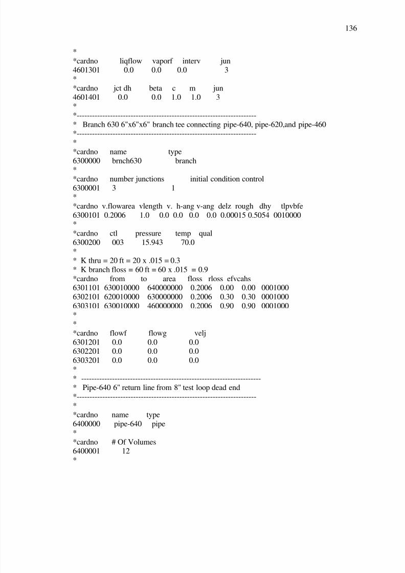
7/29/2019 Simulation and Validation of Two-component Flow in a Void Recircu
http://slidepdf.com/reader/full/simulation-and-validation-of-two-component-flow-in-a-void-recircu 152/171
136
*
*cardno liqflow vaporf interv jun4601301 0.0 0.0 0.0 3
*
*cardno jct dh beta c m jun
4601401 0.0 0.0 1.0 1.0 3*
*----------------------------------------------------------------------
* Branch 630 6"x6"x6" branch tee connecting pipe-640, pipe-620,and pipe-460*----------------------------------------------------------------------
*
*cardno name type
6300000 brnch630 branch*
*cardno number junctions initial condition control
6300001 3 1
**cardno v.flowarea vlength v. h-ang v-ang delz rough dhy tlpvbfe
6300101 0.2006 1.0 0.0 0.0 0.0 0.0 0.00015 0.5054 0010000*
*cardno ctl pressure temp qual
6300200 003 15.943 70.0
** K thru = 20 ft = 20 x .015 = 0.3
* K branch floss = 60 ft = 60 x .015 = 0.9
*cardno from to area floss rloss efvcahs6301101 630010000 640000000 0.2006 0.00 0.00 0001000
6302101 620010000 630000000 0.2006 0.30 0.30 0001000
6303101 630010000 460000000 0.2006 0.90 0.90 0001000
**
*cardno flowf flowg velj
6301201 0.0 0.0 0.06302201 0.0 0.0 0.0
6303201 0.0 0.0 0.0
*
* ----------------------------------------------------------------------* Pipe-640 6" return line from 8" test loop dead end
*----------------------------------------------------------------------
**cardno name type
6400000 pipe-640 pipe
*
*cardno # Of Volumes6400001 12
*

7/29/2019 Simulation and Validation of Two-component Flow in a Void Recircu
http://slidepdf.com/reader/full/simulation-and-validation-of-two-component-flow-in-a-void-recircu 153/171
137
*cardno Volume Flow Area Volume Number
6400101 0.2006 12*
*cardno Junction Flow Area Junction Number
6400201 0.2006 11
**cardno volume lengths Volume Number
6400301 0.506 12
**cardno Volume Volume Number
6400401 0.0 12
*
*cardno Vertical Angle Volume Number
6400601 0.0 12
*
*cardno rough dhyd Volume Number6400801 0.00015 0.5054 12
**cardno kfor krev Junction Number
6400901 0.0 0.0 5
6400902 0.45 0.45 6
6400903 0.0 0.0 11*
*cardno tlpvbfe Volume Number
6401001 0010000 12*
*cardno efvchas Junction Number
6401101 0001000 11
**cardno ic press temp qual W5 W6 vol.
6401201 3 15.943 70.0 0.0 0.0 0.0 12
**cardno vel/flow
6401300 1
* W1 = mass flow ic
**cardno liqflow vaporf interv jun
6401301 0.0 0.0 0.0 11
**cardno jct dh beta c m jun
6401401 0.0 0.0 1.0 1.0 11
*
** ----------------------------------------------------------------------
* Pipe-620 6" return line - 6" test loop branch630 to 4" test loop branch610
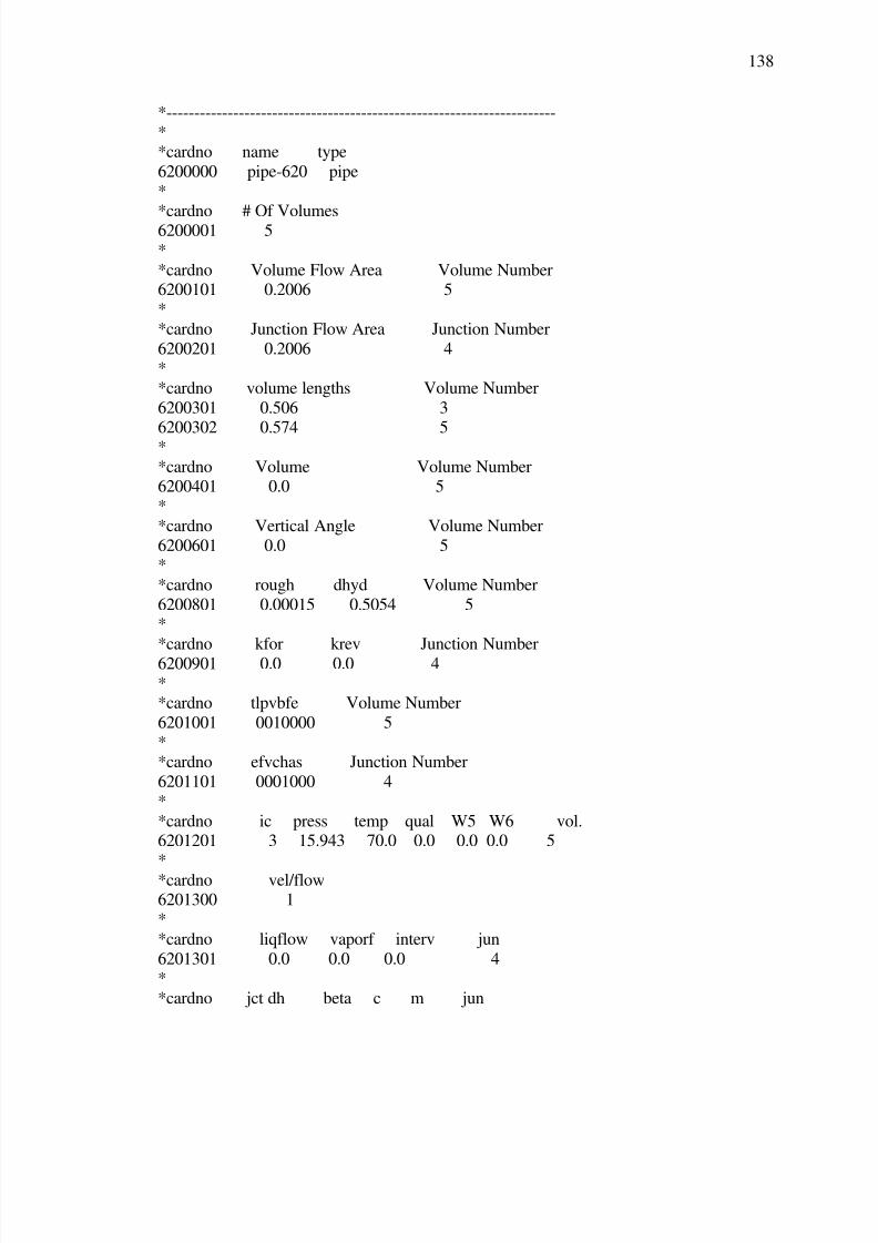
7/29/2019 Simulation and Validation of Two-component Flow in a Void Recircu
http://slidepdf.com/reader/full/simulation-and-validation-of-two-component-flow-in-a-void-recircu 154/171
138
*----------------------------------------------------------------------
**cardno name type
6200000 pipe-620 pipe
*
*cardno # Of Volumes6200001 5
*
*cardno Volume Flow Area Volume Number6200101 0.2006 5
*
*cardno Junction Flow Area Junction Number
6200201 0.2006 4*
*cardno volume lengths Volume Number
6200301 0.506 3
6200302 0.574 5*
*cardno Volume Volume Number6200401 0.0 5
*
*cardno Vertical Angle Volume Number
6200601 0.0 5*
*cardno rough dhyd Volume Number
6200801 0.00015 0.5054 5*
*cardno kfor krev Junction Number
6200901 0.0 0.0 4
**cardno tlpvbfe Volume Number
6201001 0010000 5
**cardno efvchas Junction Number
6201101 0001000 4
*
*cardno ic press temp qual W5 W6 vol.6201201 3 15.943 70.0 0.0 0.0 0.0 5
*
*cardno vel/flow6201300 1
*
*cardno liqflow vaporf interv jun
6201301 0.0 0.0 0.0 4*
*cardno jct dh beta c m jun
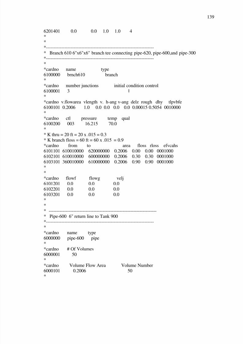
7/29/2019 Simulation and Validation of Two-component Flow in a Void Recircu
http://slidepdf.com/reader/full/simulation-and-validation-of-two-component-flow-in-a-void-recircu 155/171
139
6201401 0.0 0.0 1.0 1.0 4
**
*----------------------------------------------------------------------
* Branch 610 6"x6"x6" branch tee connecting pipe-620, pipe-600,and pipe-300
*----------------------------------------------------------------------*
*cardno name type
6100000 brnch610 branch*
*cardno number junctions initial condition control
6100001 3 1
**cardno v.flowarea vlength v. h-ang v-ang delz rough dhy tlpvbfe
6100101 0.2006 1.0 0.0 0.0 0.0 0.0 0.00015 0.5054 0010000
*
*cardno ctl pressure temp qual6100200 003 16.215 70.0
** K thru = 20 ft = 20 x .015 = 0.3
* K branch floss = 60 ft = 60 x .015 = 0.9
*cardno from to area floss rloss efvcahs
6101101 610010000 620000000 0.2006 0.00 0.00 00010006102101 610010000 600000000 0.2006 0.30 0.30 0001000
6103101 360010000 610000000 0.2006 0.90 0.90 0001000
**
*cardno flowf flowg velj
6101201 0.0 0.0 0.0
6102201 0.0 0.0 0.06103201 0.0 0.0 0.0
*
** ----------------------------------------------------------------------
* Pipe-600 6" return line to Tank 900
*----------------------------------------------------------------------
**cardno name type
6000000 pipe-600 pipe
**cardno # Of Volumes
6000001 50
*
*cardno Volume Flow Area Volume Number6000101 0.2006 50
*
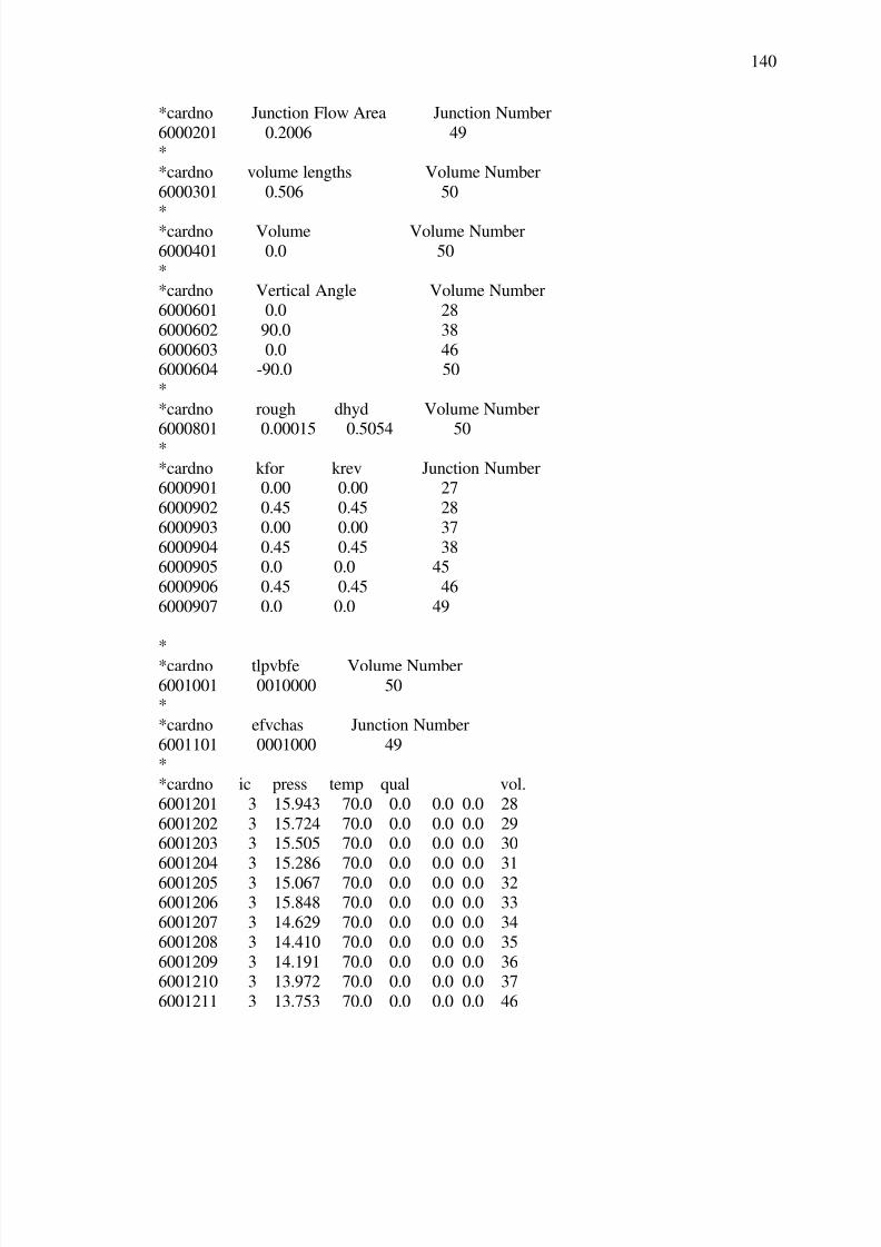
7/29/2019 Simulation and Validation of Two-component Flow in a Void Recircu
http://slidepdf.com/reader/full/simulation-and-validation-of-two-component-flow-in-a-void-recircu 156/171
140
*cardno Junction Flow Area Junction Number
6000201 0.2006 49*
*cardno volume lengths Volume Number
6000301 0.506 50
**cardno Volume Volume Number
6000401 0.0 50
**cardno Vertical Angle Volume Number
6000601 0.0 28
6000602 90.0 38
6000603 0.0 466000604 -90.0 50
*
*cardno rough dhyd Volume Number
6000801 0.00015 0.5054 50*
*cardno kfor krev Junction Number6000901 0.00 0.00 27
6000902 0.45 0.45 28
6000903 0.00 0.00 37
6000904 0.45 0.45 386000905 0.0 0.0 45
6000906 0.45 0.45 46
6000907 0.0 0.0 49
*
*cardno tlpvbfe Volume Number
6001001 0010000 50*
*cardno efvchas Junction Number
6001101 0001000 49*
*cardno ic press temp qual vol.
6001201 3 15.943 70.0 0.0 0.0 0.0 28
6001202 3 15.724 70.0 0.0 0.0 0.0 296001203 3 15.505 70.0 0.0 0.0 0.0 30
6001204 3 15.286 70.0 0.0 0.0 0.0 31
6001205 3 15.067 70.0 0.0 0.0 0.0 326001206 3 15.848 70.0 0.0 0.0 0.0 33
6001207 3 14.629 70.0 0.0 0.0 0.0 34
6001208 3 14.410 70.0 0.0 0.0 0.0 35
6001209 3 14.191 70.0 0.0 0.0 0.0 366001210 3 13.972 70.0 0.0 0.0 0.0 37
6001211 3 13.753 70.0 0.0 0.0 0.0 46
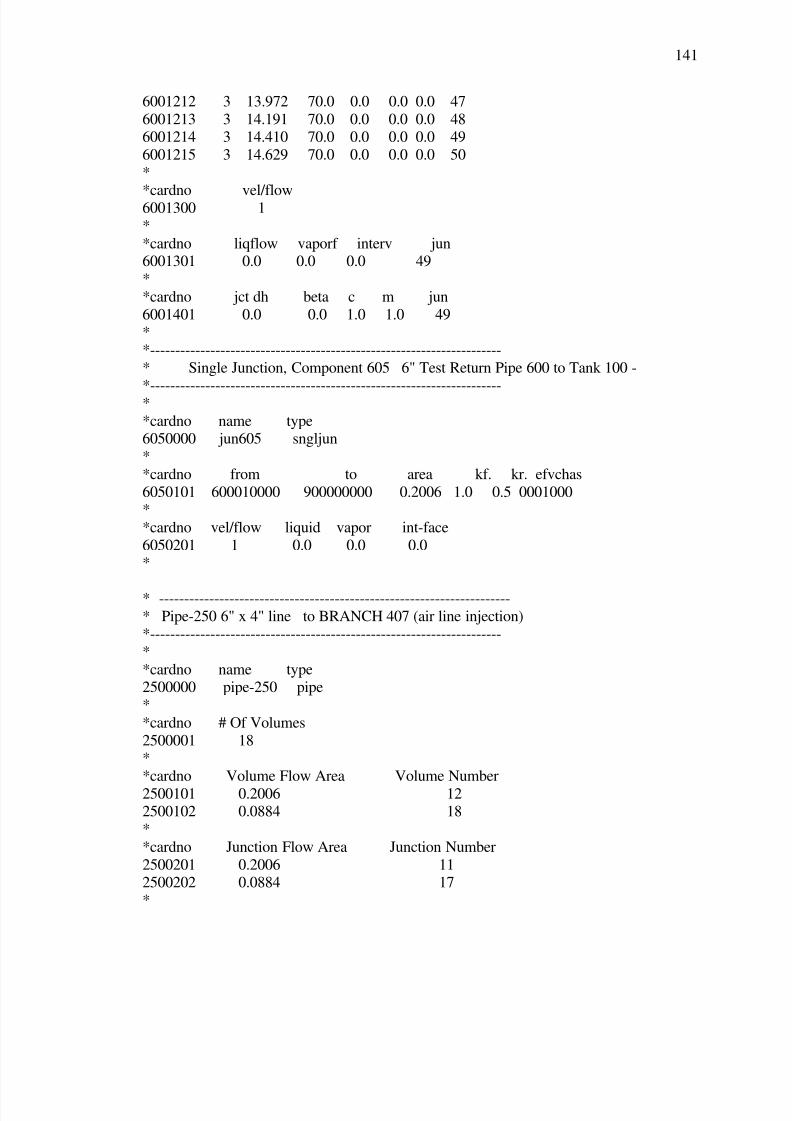
7/29/2019 Simulation and Validation of Two-component Flow in a Void Recircu
http://slidepdf.com/reader/full/simulation-and-validation-of-two-component-flow-in-a-void-recircu 157/171
141
6001212 3 13.972 70.0 0.0 0.0 0.0 47
6001213 3 14.191 70.0 0.0 0.0 0.0 486001214 3 14.410 70.0 0.0 0.0 0.0 49
6001215 3 14.629 70.0 0.0 0.0 0.0 50
*
*cardno vel/flow6001300 1
*
*cardno liqflow vaporf interv jun6001301 0.0 0.0 0.0 49
*
*cardno jct dh beta c m jun
6001401 0.0 0.0 1.0 1.0 49*
*----------------------------------------------------------------------
* Single Junction, Component 605 6" Test Return Pipe 600 to Tank 100 -
*----------------------------------------------------------------------*
*cardno name type6050000 jun605 sngljun
*
*cardno from to area kf. kr. efvchas
6050101 600010000 900000000 0.2006 1.0 0.5 0001000*
*cardno vel/flow liquid vapor int-face
6050201 1 0.0 0.0 0.0*
* ----------------------------------------------------------------------
* Pipe-250 6" x 4" line to BRANCH 407 (air line injection)*----------------------------------------------------------------------
*
*cardno name type2500000 pipe-250 pipe
*
*cardno # Of Volumes
2500001 18*
*cardno Volume Flow Area Volume Number
2500101 0.2006 122500102 0.0884 18
*
*cardno Junction Flow Area Junction Number
2500201 0.2006 112500202 0.0884 17
*
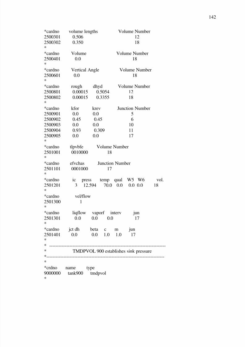
7/29/2019 Simulation and Validation of Two-component Flow in a Void Recircu
http://slidepdf.com/reader/full/simulation-and-validation-of-two-component-flow-in-a-void-recircu 158/171
142
*cardno volume lengths Volume Number
2500301 0.506 122500302 0.350 18
*
*cardno Volume Volume Number
2500401 0.0 18*
*cardno Vertical Angle Volume Number
2500601 0.0 18*
*cardno rough dhyd Volume Number
2500801 0.00015 0.5054 12
2500802 0.00015 0.3355 18*
*cardno kfor krev Junction Number
2500901 0.0 0.0 5
2500902 0.45 0.45 62500903 0.0 0.0 10
2500904 0.93 0.309 112500905 0.0 0.0 17
*
*cardno tlpvbfe Volume Number
2501001 0010000 18*
*cardno efvchas Junction Number
2501101 0001000 17*
*cardno ic press temp qual W5 W6 vol.
2501201 3 12.594 70.0 0.0 0.0 0.0 18
**cardno vel/flow
2501300 1
**cardno liqflow vaporf interv jun
2501301 0.0 0.0 0.0 17
*
*cardno jct dh beta c m jun2501401 0.0 0.0 1.0 1.0 17
*
* ---------------------------------------------------------------------------* TMDPVOL 900 establishes sink pressure
*----------------------------------------------------------------------------
*
*crdno name type9000000 tank900 tmdpvol
*

7/29/2019 Simulation and Validation of Two-component Flow in a Void Recircu
http://slidepdf.com/reader/full/simulation-and-validation-of-two-component-flow-in-a-void-recircu 159/171
143
*cardno area length volume
9000101 10.0 1.0e6 0.0*
*cardno azim angle incl. Angle deltaz
9000102 0 0.0 0.0
**cardno roughness hyddia pvbfe
9000103 0.00015 0.0 00010
**cardno ebt trip search var
9000200 003
*
*cardno time Pressure Temperature9000201 0.00 14.7 70.0
9000202 5.00 14.7 70.0
9000203 1.0e6 14.7 70.0
*.
* end of input
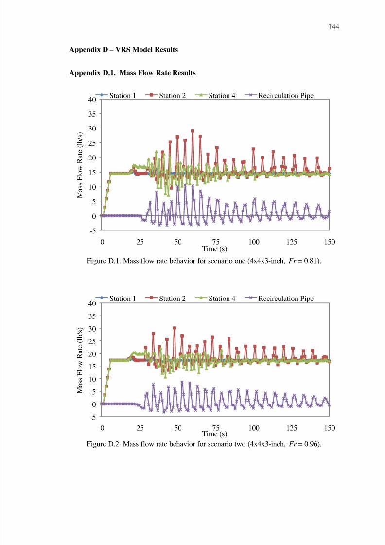
7/29/2019 Simulation and Validation of Two-component Flow in a Void Recircu
http://slidepdf.com/reader/full/simulation-and-validation-of-two-component-flow-in-a-void-recircu 160/171
144
Appendix D – VRS Model Results
Appendix D.1. Mass Flow Rate Results
Figure D.1. Mass flow rate behavior for scenario one (4x4x3-inch, Fr = 0.81).
Figure D.2. Mass flow rate behavior for scenario two (4x4x3-inch, Fr = 0.96).
-5
0
510
15
20
25
30
35
40
0 25 50 75 100 125 150
M a
s s F l o w R a t e ( l b / s )
Time (s)
Station 1 Station 2 Station 4 Recirculation Pipe
-5
0
510
15
20
25
30
35
40
0 25 50 75 100 125 150
M a s s F l o w R a t e ( l b / s )
Time (s)
Station 1 Station 2 Station 4 Recirculation Pipe
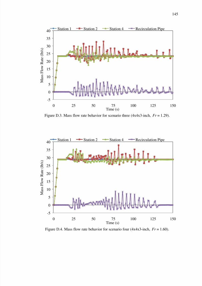
7/29/2019 Simulation and Validation of Two-component Flow in a Void Recircu
http://slidepdf.com/reader/full/simulation-and-validation-of-two-component-flow-in-a-void-recircu 161/171
145
Figure D.3. Mass flow rate behavior for scenario three (4x4x3-inch, Fr = 1.29).
Figure D.4. Mass flow rate behavior for scenario four (4x4x3-inch, Fr = 1.60).
-5
0
5
10
15
20
25
30
35
40
0 25 50 75 100 125 150
M a s s F l o w R a t e ( l b / s )
Time (s)
Station 1 Station 2 Station 4 Recirculation Pipe
-5
0
5
10
15
20
25
30
35
40
0 25 50 75 100 125 150
M a s s F l o w R a t e ( l b / s )
Time (s)
Station 1 Station 2 Station 4 Recirculation Pipe
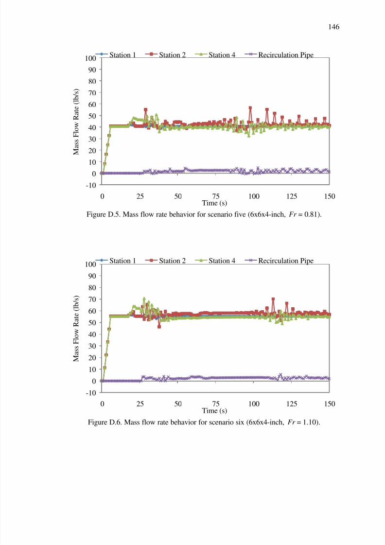
7/29/2019 Simulation and Validation of Two-component Flow in a Void Recircu
http://slidepdf.com/reader/full/simulation-and-validation-of-two-component-flow-in-a-void-recircu 162/171
146
Figure D.5. Mass flow rate behavior for scenario five (6x6x4-inch, Fr = 0.81).
Figure D.6. Mass flow rate behavior for scenario six (6x6x4-inch, Fr = 1.10).
-10
0
10
20
30
40
50
6070
80
90
100
0 25 50 75 100 125 150
M a s s F l o w R a t e ( l b / s )
Time (s)
Station 1 Station 2 Station 4 Recirculation Pipe
-100
10
20
30
40
50
60
70
80
90
100
0 25 50 75 100 125 150
M a s s F l o w R a t e ( l b / s )
Time (s)
Station 1 Station 2 Station 4 Recirculation Pipe
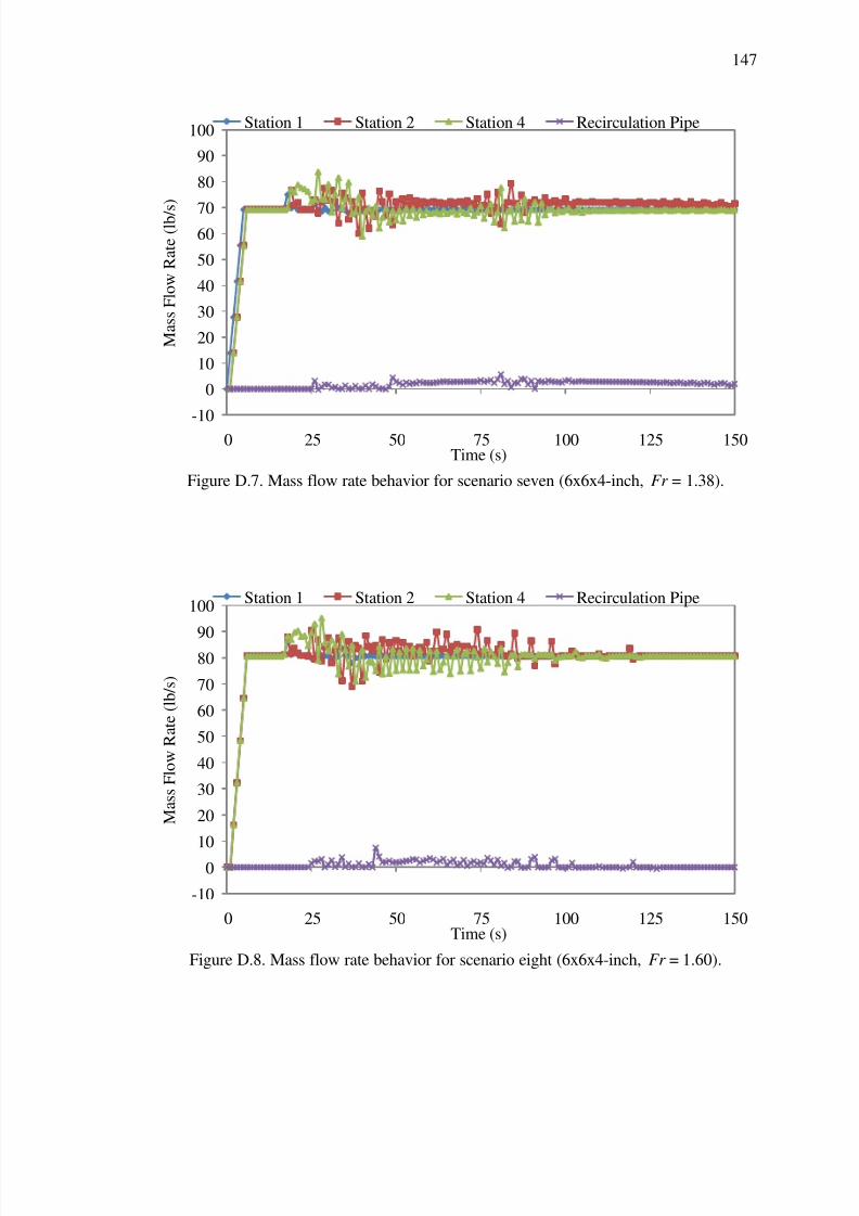
7/29/2019 Simulation and Validation of Two-component Flow in a Void Recircu
http://slidepdf.com/reader/full/simulation-and-validation-of-two-component-flow-in-a-void-recircu 163/171
147
Figure D.7. Mass flow rate behavior for scenario seven (6x6x4-inch, Fr = 1.38).
Figure D.8. Mass flow rate behavior for scenario eight (6x6x4-inch, Fr = 1.60).
-10
0
10
20
30
40
50
6070
80
90
100
0 25 50 75 100 125 150
M a s s F l o w R a t e ( l b / s )
Time (s)
Station 1 Station 2 Station 4 Recirculation Pipe
-10
0
10
20
30
40
50
60
70
8090
100
0 25 50 75 100 125 150
M a s s F l o w R a t e ( l b / s )
Time (s)
Station 1 Station 2 Station 4 Recirculation Pipe
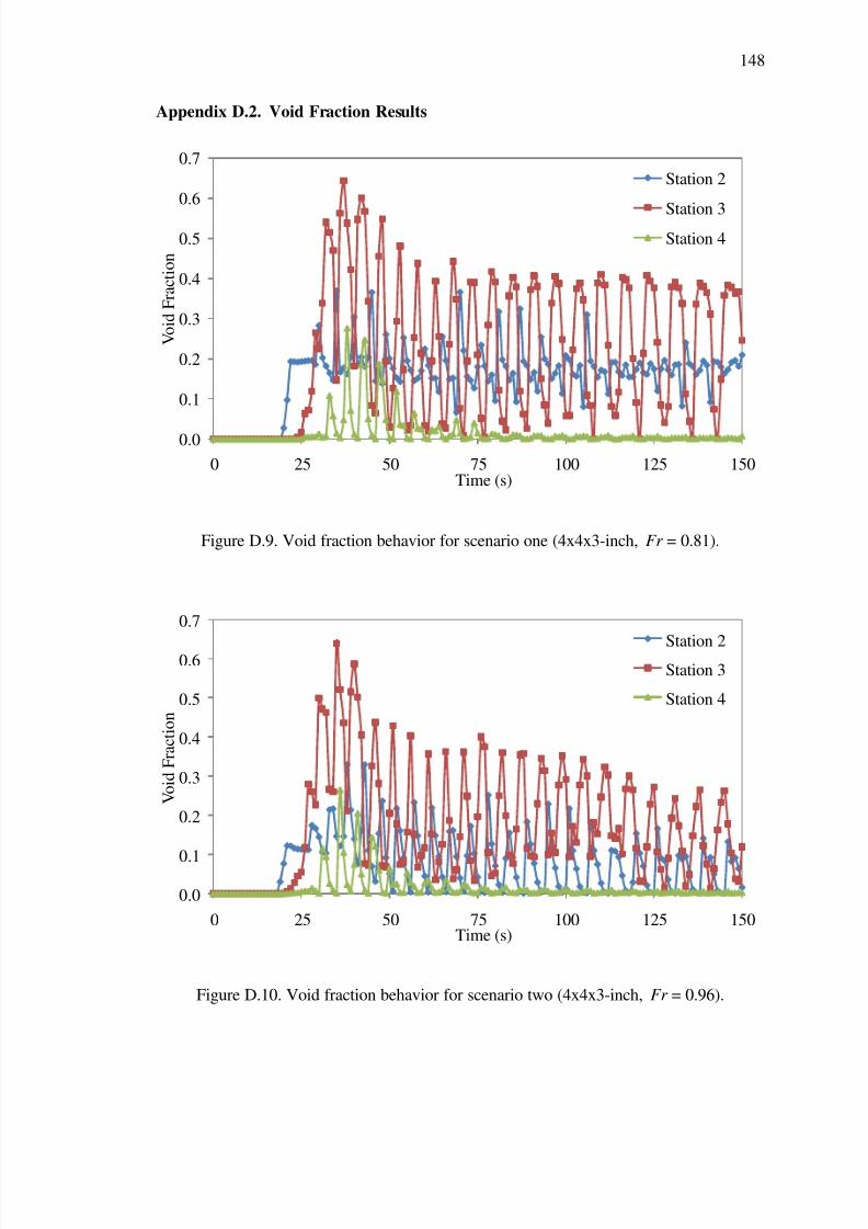
7/29/2019 Simulation and Validation of Two-component Flow in a Void Recircu
http://slidepdf.com/reader/full/simulation-and-validation-of-two-component-flow-in-a-void-recircu 164/171
148
Appendix D.2. Void Fraction Results
Figure D.9. Void fraction behavior for scenario one (4x4x3-inch, Fr = 0.81).
Figure D.10. Void fraction behavior for scenario two (4x4x3-inch, Fr = 0.96).
0.0
0.1
0.2
0.3
0.4
0.5
0.6
0.7
0 25 50 75 100 125 150
V o i d F r a c t i o n
Time (s)
Station 2
Station 3Station 4
0.0
0.1
0.2
0.3
0.4
0.5
0.6
0.7
0 25 50 75 100 125 150
V o i d F r a c t i o n
Time (s)
Station 2Station 3
Station 4
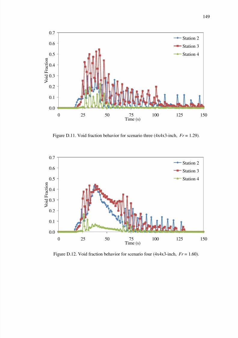
7/29/2019 Simulation and Validation of Two-component Flow in a Void Recircu
http://slidepdf.com/reader/full/simulation-and-validation-of-two-component-flow-in-a-void-recircu 165/171
149
Figure D.11. Void fraction behavior for scenario three (4x4x3-inch, Fr = 1.29).
Figure D.12. Void fraction behavior for scenario four (4x4x3-inch, Fr = 1.60).
0.0
0.1
0.2
0.3
0.4
0.5
0.6
0.7
0 25 50 75 100 125 150
V o i d F r a c t i o n
Time (s)
Station 2
Station 3
Station 4
0.0
0.1
0.2
0.3
0.4
0.5
0.6
0.7
0 25 50 75 100 125 150
V o i d F r a c t i o n
Time (s)
Station 2
Station 3
Station 4

7/29/2019 Simulation and Validation of Two-component Flow in a Void Recircu
http://slidepdf.com/reader/full/simulation-and-validation-of-two-component-flow-in-a-void-recircu 166/171
150
Figure D.13. Void fraction behavior for scenario five (6x6x4-inch, Fr = 0.81).
Figure D.14. Void fraction behavior for scenario six (6x6x4-inch, Fr = 1.10).
0.0
0.1
0.2
0.3
0.4
0.5
0.6
0.7
0 25 50 75 100 125 150
V o i d F r a c t i o n
Time (s)
Station 2
Station 3
Station 4
0.0
0.1
0.2
0.3
0.4
0.5
0.6
0.7
0 25 50 75 100 125 150
V o i d F r a c t i o n
Time (s)
Station 2
Station 3
Station 4
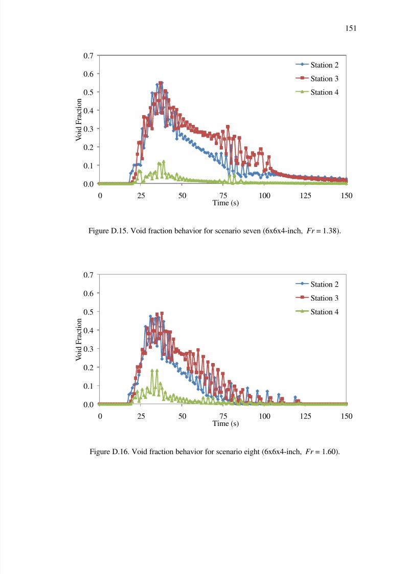
7/29/2019 Simulation and Validation of Two-component Flow in a Void Recircu
http://slidepdf.com/reader/full/simulation-and-validation-of-two-component-flow-in-a-void-recircu 167/171
151
Figure D.15. Void fraction behavior for scenario seven (6x6x4-inch, Fr = 1.38).
Figure D.16. Void fraction behavior for scenario eight (6x6x4-inch, Fr = 1.60).
0.0
0.1
0.2
0.3
0.4
0.5
0.6
0.7
0 25 50 75 100 125 150
V o i d F r a c t i o n
Time (s)
Station 2
Station 3
Station 4
0.0
0.1
0.2
0.3
0.4
0.5
0.6
0.7
0 25 50 75 100 125 150
V o i d F r a c t i o n
Time (s)
Station 2
Station 3Station 4

7/29/2019 Simulation and Validation of Two-component Flow in a Void Recircu
http://slidepdf.com/reader/full/simulation-and-validation-of-two-component-flow-in-a-void-recircu 168/171
152
Appendix E – VRS Simulation and Experimental Void Fraction Validation
Figure E.1. Void fraction validation for scenario one (4x4x3-inch, Fr = 0.81).
Figure E.2. Void fraction validation for scenario two (4x4x3-inch, Fr = 0.96).
0.0
0.1
0.2
0.3
0.4
0.5
0.6
0.7
0 1 2 3 4 5
V o i d F r a c t i o n
Station No.
Experimental
Model
0.0
0.1
0.2
0.3
0.4
0.5
0.6
0.7
0 1 2 3 4 5
V o i d F r a c t i o n
Station No.
Experimental
Model

7/29/2019 Simulation and Validation of Two-component Flow in a Void Recircu
http://slidepdf.com/reader/full/simulation-and-validation-of-two-component-flow-in-a-void-recircu 169/171
153
Figure E.3. Void fraction validation for scenario three (4x4x3-inch, Fr = 1.29).
Figure E.4. Void fraction validation for scenario four (4x4x3-inch, Fr = 1.60).
0.0
0.1
0.2
0.3
0.4
0.5
0.6
0.7
0 1 2 3 4 5
V o i d F r a c t i o n
Station No.
Experimental
Model
0.0
0.1
0.2
0.3
0.4
0.5
0.6
0.7
0 1 2 3 4 5
V o i d F r a c t i o n
Station No.
Experimental
Model
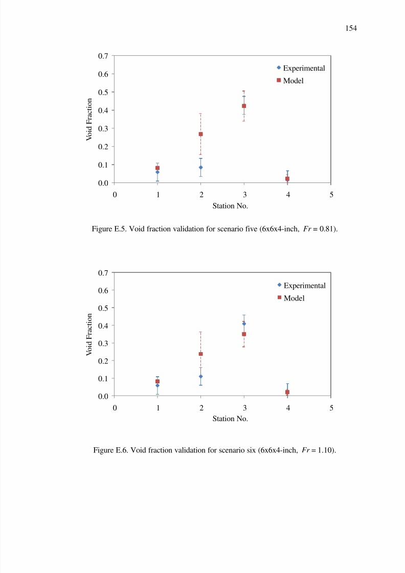
7/29/2019 Simulation and Validation of Two-component Flow in a Void Recircu
http://slidepdf.com/reader/full/simulation-and-validation-of-two-component-flow-in-a-void-recircu 170/171
154
Figure E.5. Void fraction validation for scenario five (6x6x4-inch, Fr = 0.81).
Figure E.6. Void fraction validation for scenario six (6x6x4-inch, Fr = 1.10).
0.0
0.1
0.2
0.3
0.4
0.5
0.6
0.7
0 1 2 3 4 5
V o i d F r a c t i o n
Station No.
Experimental
Model
0.0
0.1
0.2
0.3
0.4
0.5
0.6
0.7
0 1 2 3 4 5
V o i d F r a c t i o n
Station No.
Experimental
Model

7/29/2019 Simulation and Validation of Two-component Flow in a Void Recircu
http://slidepdf.com/reader/full/simulation-and-validation-of-two-component-flow-in-a-void-recircu 171/171
155
Figure E.7. Void fraction validation for scenario seven (6x6x4-inch, Fr = 1.38).
0.0
0.1
0.2
0.3
0.4
0.5
0.6
0.7
0 1 2 3 4 5
V o i d F r a c t i o n
Station No.
Experimental
Model