SIMULA TION AS A RESOURCE RECOVERY

PLANT DESIGN TOOL

H. G. RIGO CSI Resource Systems, Inc.

Boston, Massachusetts

ABSTRACT

After a short general introduction to Monte Carlo simulation techniques and the mathematical formulation of necessary stochastic variables, var­ious waste-to-energy plant configurations are stud­ied using Monte Carlo simulation. A method for predicting long-tenn plant technical performance which considers the statistical nature of waste de­liveries and plant operations is presented. The worked examples investigate trade-offs between capacity

and redundancy design parameters. The results can be combined with standard cost engineering tech­niques to quantify plant economic performance.

INTRODUCTION

Modem resource recovery plants are expensive

facilities to build and maintain. To minimize the cost of these facilities while continuing to provide environmentally sound and fiscally responsible waste management services, it is important to strike the proper balance between plant design capacity and waste stream characteristics.

Traditional engineering calculations for resource recovery plants are deterministic in nature and assume that the design criteria are adequately represented by average or peak processing require­ments and properties. However, such static treat­ment of highly variable waste and processing char­acteristics can lead to inappropriately sized plants. Fortunately, a number of techniques can be em­ployed to account for the variable nature of waste

characteristics and plant processing capabilities. This paper explores one type of analysis, Monte Carlo simulation. Monte Carlo techniques also allow designers to simulate the long-term perfoIlIl­ance of a particular plant configuration during the process engineering phase rather than after the plant is built.

Monte Carlo simulation * is performed by re­peated analysis of a system during which the in­puts and plant status are allowed to vary between each step according to known statistical distribu­tion of the input variables. Repeated sampling us­ing random numbers instead of dice or a roulette wheel to randomly select the value for every stochastic variable at each step of the simulation will produce predicted operating results also hav­ing a statistical distribution. After sufficient trials, the resulting plant operating estimates will charac­terize the plant's performance distribution.

When systems include components like surge bins and storage pits whose ability to deliver or re­ceive waste is dependent on the entire plant his­tory up to that point in time, analysis can indicate that all incoming waste will be processed easily. However, a series of high waste delivery days and/or concurrent forced outages is likely, making it necessary to bypass waste to the landfill.

·In this analysis, the plant status at the end of the pre­

ceding time step becomes the initial condition for the cur­

rent time step. Since the path followed to arrive at a par­

ticular point of time has no bearing on the next estimate

of the stochastic variables, this is a Markov analysis. A more extensive discussion of this analysis can be found in the appendix.

459

When the stochastic variables are solid waste characteristics, furnace scheduled and forced outage rates, and refuse-derived fuel (RDF) pro­cessing line up and down time distributions, the effect of varying the plant's receiving, processing line, and boiler capacities can be studied. By anal­yzing a proposed system for its ability to process the delivered waste and the amount of time the furnaces will be operated, the technical parameters necessary to characterize a plant's output (consider­ing uncertainty) can be predicted. Once the plant's output is determined, revenues from the processed waste and disposal costs for unprocessed waste and residue can be estimated. Conventional cost engi­neering techniques can be used to determine the net cost of a design alternative.

Such simulations provide a more firm basis for estimating system costs and revenues than do sensi­tivity analyses. In the case of waste processing plants, the input parameters all vary simultaneous­ly along with plant performance and operating status. Sensitivity analysis varies only one param­eter at a time. In a Monte Carlo simulation, the center of the response distribution is the system performance when all input variables are at tl;eir average values, but the range of results is much

\

narrower than what would result from estimates based on the extreme values of the input variables. This is because it is highly unlikely that every variable would be simultaneously at an extreme value. The Monte Carlo simulation recognizes both probability and value. The technique provides a practical means of analyzing very complex stochas­tic problems.

To provide a greater understanding of the Monte Carlo technique, two example problems are pre­sented in the balance of this paper. Some of the information developed by the simulation is dis­cussed.

A MODULAR COMBUSTION UNIT DESIGN PROBLEM

Displayed in Fig. 1 is a flowchart for a relative­ly simple waste-to-energy plant composed of a tip­ping floor with a fixed capacity and three or four identical modular combustion units (MCUs). Each MCU has its own waste heat boiler. For Simplicity, it is assumed that the plant operates 5 days/week, 24 hr/day. Each MCU is brought down on the week­end for routine maintenance and municipal solid waste (MSW) is delivered 5 days/week. A.5 percent forced outage rate, the average weekday waste de-

460

livery (x) with a standard deviation (s) equal to 25 percent of the average daily and Saturday deliveries equal to one quarter of the average daily delivery is specified. The effect on the receiving area and indi­vidual unit capacities will both be studied using Monte Carlo simulation techniques.

The simulation proceeded as follows. The first step was to estimate the amount of waste to be de­livered to the plant using a random number and the mean and standard deviation for the day of the week as explained in the appendix. That estimated amount was then added to the waste already in the plant. Because most waste is delivered during a relatively short period each day, any tonnage in excess of remaining plant storage capacity was accumulated as bypassed waste to be sent to a landfill.

Next, the status of the plant (the number of units scheduled to be operating) and the actual number of units that were up, were determined by using a random number and a "look-up" table (dis­cussed under Combustion Unit Availability in the appendix). The waste on the tipping floor was then reduced by the daily "up" processing capacity. If there was insufficient waste to operate the units at their rated capacity, all unit capacities were fust reduced to no less than 60 percent of their rating, an assumed turn-down ratio. If there was still in­sufficient waste, units were sequentially taken off­line until only those units necessary to process the available waste were utilized. As units were down because of either scheduled or forced outage or lack of waste, unit-hours of down time were accu­mulated.

The waste bypassed from the plant was accu­mulated and divided by the total tons delivered to calculate the bypass ratio. The total number of unit-hours of down time were divided by the unit­hours simulated (number of units times hours simulated) to compute the estimated boiler down time ratio. The simulation was repeated day by day until the bypass and unit down time ratios stabil­ized.

SOLID WASTE x & s KNOWN

WEEKDAYS - 5(, s SATURDAY - 15(, Is SUNDAY - 0, °

RECEIVING

MCUs CAPACITY KNOWN

T CAPACITY 1-----1�-I KNOWN

, ' , ' , I L_ •• J

FIG. 1 PROCESS FLOW DIAGRAM FOR THE THREE OR FOUR MCU PROBLEM

'" '"

@ � co

if ->- <D '" -

.W .. t; -� '" -w

51 -' '"

� co

g <D a: a.

u. ..

0

2R '"

100 150

3-49 TPO UNITS Wi 500 T PIT

4-36 TPD UNITS Wi 500 T PIT

I I •

I I I I

I I I ,

I I I I

I .L4-49 TPO ,. " UNITS wI

" I 300 T PIT I I

J I I I

I "4-49 TPO UNITS ,/ / WI 500 T PIT

I I I ,

I / / /

, I -' / - /

� .. ; " /

200

T OF PROCESSIBLE WASTE DELIVERED PER WEEKDAY

FIG. 2 COMPARISON OF ALTERNATIVE PLANT

CONFIGURATIONS

Shown in Fig. 2 are the results of Markov-type Monte Carlo simulations for four different plant . configurations that use commercially available equipment. A plant with three 40-TPD * units be­haves almost like a plant with four 36-TPD units with an equivalently sized pit or storage/receiving area. Increasing the size of the pit increases the average daily arrival rate at which waste begins to bypass the plant.

Figure 2 can be used to compare the relative merits of different plant configurations on both seasonally varying waste streams and the future requirements of growing waste sheds. A worked example problem is presented in Table 1, estimat­ing the waste bypassed for a specific plant (4 by 36 TPD) and tipping floor (500 T) configuration and the equivalent receiving days per month. The equivalent working days are the sum of week days plus one quarter of the Saturdays to account for different weekday and weekend deliveries. The estimated bypass is 8.9 percent of the waste de­livered. Similar calculations for other plant con­figurations result in an estimated 0.2 percent by­pass for the 4 by 49 TPD case with a 500 T pit and a 1.1 percent bypass for the 4 by 49 TPD unit case with a 300 T pit. Hence, the number of units, their capacity, and the receiving area/storage ca­pacity of the plant are all important variables to be optimized during system development.

The usefulness of the results of a few simula­tions can be greatly enhanced by non dimensional­izing results like those presented in Fig. 1. This can be accomplished by using the average weekly pro­cessing capacity (hours/week x TPH/unit x num-

• Because all inputs have been normalized to T of MSW

input, these results are equally valid if TPD is read as

either metric or English tons. A metric ton is approxi­

mately 1.1 English ton.

461

TABLE 1 ESTIMATED ANNUAL BYPASS FOR A

4 BY 36 TPD MCU PLANT WITH A 500-T PIT

Equivalent Average Work Weekly •

Daysl Delivery Percent T T Month Months (TPW) Bypass Received Bypassed

Oct. 24 145 1.6 3,480 56

Nov. 23 143 1.0 3,289 33

Dec. 22% 143 1.0 3,182 32

Jan. 24 188 21.8 4,512 984

Feb. 22 181 18.5 3,982 737

March 22% 173 13.7 3,849 527

April 23 175 15.0 4,025 604

May 23% 158 5.3 3,674 195

June 22 164 8.5 3,608 307

July 23 158 5.3 3,634 193

August 22% 155 4.5 3,449 155

Sept. 23 150 3.0 3,450 104

44,133 3,924

Annual T Processed = 40,209

Annual Bypass = 8.9 percent

ber of units x availability) as the denominator, and by using variables which describe average week-ly MSW deliveries and receiving/storage area capac-ity as the numerator, as shown below.

_ average weekly MSW delivery '" = average weekly processing capacity

For: 0.5 < '" < 1.5

d - tons of pit capacity an 1/>-- average weekly finll plant capacity

For: 0.1 < I/> < 1.0, •

Using Eqs. (10) and (11) along with other simu-lations, Fig. 3 was developed for a plant with four installed combustion units scheduled to operate 5 days per week and receiving waste each weekday and 1/4 day on Saturday. Two major results of this simulation are presented in Fig. 3. First, the average unit down time is plotted. The percent of boiler down time becomes asymptotic to the unit's (and plant's) forced outage rate as waste delivery to the plant is increased. This is due to routine mainte­

nance being scheduled during weekend shutdowns. Second, waste bypass is plotted. Waste bypasses the plant when the receiving area is full; this can be the result of either a series of high delivery days or a series of coincidental forced outages.

Curves like Fig. 3 can be developed for many general plant configurations. Each curve is appli­cable to specific numbers of units, availability and operating schedule assumptions, and a specific statistical deSCription of the waste arrival rate. Such

general curves can be very useful for initially screen­ing alternatives. However, once a configuration has

been selected for further investigation, a site-spe­cific simulation which uses local waste delivery characteristics and equipment-specific operating data is needed to provide an accurate estimate of long-term plant performance. These technical per­formance predictions are coupled with energy balances, cost engineering outputs, and locally deter­mined bypassed waste disposal costs and product

o 0.25 0.50 lOO 1.25 l50 1'. AVG. WEEKLY DELIVERY/ AVG. WEEKLY

PROCESS CAPACIT Y

FIG.3 GENERALIZED FOUR UNIT MCU PERFOR­MANCE CURVE, FIVE DAY PER WEEK OPERATION

sales prices to establish the probable cost of dis­posal for a proposed plant. Of course, the fmal configuration will be governed by the engineer's judgment and local preferences for balancing plant costs with an acceptable degree of waste bypass.

AN RDF/DEDICATED BOILER DESIGN PROBLEM

A more complex problem is presented by an RDFjdedicated boiler plant. The plant displayed

PROCESSING LINE

SOLID WASTE

PROCESSING LINE

Solid Waste Delivery

5 J days/week 4 hours/day

i & 5 specified

Receivino Pit

F1x� tonnage specified • �ste is delivered - Was te is processed out

Process 1"9 Pi t

Fhed capacity specified (single line) Run time distribution Xo & b specified

Down time distribution xo' b specified

- Process at maxlm� capacity that does not: o exceed line rat 1ng o overflow sludge bin o exceed bol1er rating

Beilers

C\XfIu:ative probability spec.iried for 2. then I or more bol1e:-s ur

Run at maximlln capacity if line capacfty • boiler caoacity

If 1 ines + surge > 0.6 bo1 leI" up, run 'at 0.6 MCR

r�e)(t. shut down 1 line and check prey lous criteria

Reduce boiler to 0.6 HeR

Then shut down the las.t boile:".

FIG.4 GENERAL PROCESS ARRANGEMENT DIAGRAM FOR THE RDF PROBLEM

TABLE 2 TABULATED RESULTS OF THE RDF PLANT SIMULATION

Pit Surge Line MCR T T TPH TPH

5400 400 40 37.5 Variable Line Capacity problem

• � 30 50

Variable MCR problem

1 1 40

1 Variable Surge problem

• 1 • 1 000 Variable Pit problem 3600 400 t 7200 t

,

25 30 35 35 40 50

37.5

t

t

MSW xIs

1 964/490

,

1 t t

Variable MSW Delivery, Std. Deviation problem 5400 t t • 1969/245

t 1964/980 Variable average run time problem

t t t t 1969/490

Run Down Boiler Time Time Bypass Outage to/b-1 xo/b-1 Ratib Ratio

1 6.68/0.879 1 .1 1 9/1 .726 0.020±0.012 0.1 48±0.01 5

, , 0.1 85 0.1 20 0.005 0.1 03

1 1 0.273 0.043 0.1 47 0.045 0.016 0.148 0.056 0.159

0 0.194 0.003 0.1 69

+ t 0.01 1 0.1 57 0.005 0.227

• + 0.056 0.1 58 0.Q1 5 0.1 03

• + 0.021 0.141 0.075 0.170

33/0.879 t 0 0.131

462

in Fig. 4 was simulated, and the results are dis­played in Table 2 and Fig. 5-1 0.

In this example, waste is received at the plant 4 hr/day, 5% days per week. When the receiving pit is full, waste is bypassed to a sanitary landfill. This waste is processed out of storage by two RDF lines running 24 hours per day, 7 days per week. * When­ever a line is available, waste is processed at a rate limited by the amount of waste available, the capacity remaining in intermediate storage, or line capacity. The waste is then removed from inter­mediate storage for use in two boilers whose avail­abilities are governed by forced outage rates. **

Plotted in Fig. 5 are the results from seven re­peated 2,000 hour simulations of the base case [5,400 T pit, 400 T surge bin, 40 TPD individual line capacity, 37.5 TPH MSW equivalent individual boiler capacity, MSW receiving average (x) = 1 964 TPD and standard deviation(s) = 490 TPD 5 days per week and x = 491 TPD and s = 1 22 TPD on Saturday; the processing line statistical character­istics are described by the 2 parameter Weibul coefficients discussed in the appendix: to = 1 6.68 and l/b = 0.879 (up time) and to = 1 .11 9 and l/b = 1.726 (down time); forced outage rate (FOR) = 0.04]. The base case was selected because it results in some bypass and some boiler down time. Thus, it is not an optimum situation. The shaded area in Fig. 5 contains the 90 percent con­fidence interval for the true value of the bypass ratio and boiler down time - it is not an interval that contains 90 percent of the data. This ellipse is repeated on all subsequent figures to provide an indication of whether or not a specific result is likely to be different from the base case.

Shown in Fig. 6 is the effect of changing the boiler rating on the bypass ratio and the boiler down time ratio. At a combined fum weekly boiler capacity which is less than the average we�kly de­livery, the boilers operate during all of the time available and waste is b�ing bypassed because the boilers cannot burn the material. As average boiler

·Thls somewhat artificial constraint can be relaxed; how­ever, the Impacts of some design alternatives are not as easy to see in a plant with standard two-shift, 5 day/week processing.

··Insurance Inspections and annual turn-around require­

ments Indicate one 2-week and one 1-week outage per boiler. Separate simulations, rather than programming the

outage schedule Into the simulation, are easier because re­

peated runs with the program Indicate that at least 2,000 simulated hours are required to develop representative

predictions without considering the annual turn-arounds. The Inclusion of scheduled outages would extend the re­quired simulation over 100,000 cycle simulations, a pro­

hibitive simulation time.

463

"1 ��

'!1 en en � >-m :!: sa en :::<

*-.,.,

0

Ll) '"

en Ll) en -� fu :s: en 0 :::< -

�

Ll)

0

:� •

5 10 15 20 25 % BOILER DOWN TIME

FIG.5 RELATED RUNS FOR BASE CASE

.25 TPH

.30 TPH

35 TPH �37.5 TPH 50 TPH 4 TPH 5 10 15 20 25

% BOILER DOWN TIME

FIG.6 VARIABLE BOILER MCR

available capacity approaches the average weekly delivery, bypass and down time are similar to those of the base case. As boiler capacity is increased, the amount of waste bypassed approaches zero, but the frequency with which units are taken off-line be­gins to increase rapidly. Apparently, there is a hyperbolic relationship between boiler down time (which jeopardizes unit reliability and life, while increasing plant cost) and increasing waste bypass (which uses more landfill while reducing product revenues).

'" '"

�

C/) C/) 'f1 � >-CD 3: C/) ::;; Q *

'"

o 5 10

.30 TPH

�40TPH

15 20

% BOILER DOWN TIME

FIG.7 VARIABLE LINE CAPACITY

25

and availability characteristics, it appears that boiler down time and bypass can both be significantly affected by RDF line capacity. This is a compara­tively inexpensive part of a plant to enlarge and a prime candidate for optimization.

As shown in Fig. 8, for the conditions under study, plant performance is relatively insensitive to surge capacity. This apparently counter-intuitive finding is a result of the 24 hr/day operating sched­ule for the two front-end processing lines and the fact that one base case RDF processing line has sufficient capacity to keep both boilers operating at 60 percent of their maximum continuous rating. For other configurations and operating schedules, the amount of surge capacity is expected to be a significant design variable.

The effects of varying the receiving pit's size on plant performance are shown in Fig. 9. With both boilers scheduled up, a 7,200 T pit reduces bypass and down time, while a 3,600 T pit increases these characteristic parameters. During I-week outages, the larger the pit, the less by bypass. Obviously, for a 4-week scheduled outage, the pit would have to be able to hold at least 2 week's worth of accu­mulated waste as well as buffer daily surges unless there was a significant amount of reserve capacity in the boilers. The total scheduled outage time is such a small fraction of the total operating year that the infrequency of occurrences mitigates against the almost certain 50 percent bypass the last week of each 2-week outage. Hence, careful

The effect of variable line capacity is shown in Fig. 7. Under the. assumed plant operating schedule

464

o

� 400T

1000T.�O T

% BOILER DOWN TIME

FIG.8 VARIABLE SURGE

1:>5400 T

D 7200 T

7200 T ..

5 10

• NORMAL RUN TIME D ONE BOILER SCHEDULED

DOWN

.3600 T

� 5400T

15 20

% BOILER DOWN TIME

FIG. 9 VARIABLE PIT

25

planning of scheduled boiler down time throughout the year to minimize sending waste to the landfill during long scheduled outages is indicated.

The effect of changes in waste delivery on plant performance is shown in Fig. 1 0. Clearly, local waste delivery variability can have a Significant impact on plant performance. The careful deter­mination of this parameter is warranted.

til N

til

o

50%�� 25%

10 15 % BOILER DOWN TIME

, .

20 25

FIG. 10 VARIABLE DELIVERY COEFFICIENT OF

VARIANCE

Unlike the simpler pit/MCU plant case, the num­ber of physical variables is too great in RDF /dedi­cated boiler plants to permit the generation of simple trade-off curves. However, this analysis has indicated the direction of changes to be made in major system parameters in order to develop plant designs which balance waste bypass, boiler down time, and system economics. A system simulation routine can be coupled with good engineering judg­ment and some "experimental design" procedures, such as response surface methodologies (Box, Hun­ter and Hunter, 1980), to lead rapidly to an appro­priate solution to a local community's waste dis­posal problem.

CONCLUSIONS

Monte Carlo simulation can be used to study the long-term appropriateness of a plant design and to trade off investment alternatives while preparing fmal system configurations. Future applications of Monte Carlo simulation include the statistical sizing of processing components and conveyors, including variations in mass flow, waste composition, and material density .

The methodologies employed in this paper are well known in reliability, traffic, and utility load engineering circles. They also seem to be emerging in power plant design practice, but are novel in waste-to-energy plant design. As a result, this paper relied heavily on sparce data in order to begin to use Monte Carlo simulation as a tool for waste-to­energy plant configuration evaluation.

465

The author is convinced that the tool is power­ful and will enable designers to perform better as more relevant data are collected and analyzed. The data collection should include not only additional plant and component performance information, but also information on the statistiCal nature of

•

waste. Because plant operators frequently consider their facility performance data proprietary and many communities do not weigh their waste, estab­lishing the requisite data base may be difficult and not available in the immediate future. However, the simulation results are certainly informative and indicate that such a data collection effort is war­ranted.

APPENDIX:- FORMULATION OF A MARKOV MODEL

STATISTICAL DESCRIPTION OF MAJOR PLANT VARIABLES

When developing a Markov model of a resource recovery plant, a statistical description of stochastic variables and the availability of a pseudo-random number generator are essential. The latter is em­ployed to create a set of random numbers between o and 1. These random numbers can then be used in conjunction with known parameter statistics to develop a random series of values which have the same statistical distribution as the parent popula­tion for the stochastic variables. Repeated engi­neering analysis of the system using the randomly selected stochastic variable values will yield a set of results. These results defme the statistical distribu­tion of plant performance. Using the output distri­bution, the engineer can decide whether the chance or risk of some outcome is acceptable and alter his design as appropriate.

STOCHASTIC VARIABLES

WASTE DELIVERY

All of the solid waste delivery records the author has used over the last 10 years can be character­ized by normal distribution. Therefore, an adequate representation of Monday through Friday deliveries can be made if the average and standard deviation for the daily tonnage deliveries are known. Usually, the coefficient of variance for weekday deliveries (the ratio of standard deviation to average delivery) is the same as the coefficient of variation for Satur­day deliveries. Saturday deliveries, however, are usually some fraction less than one of the weekday

deliveries. Additional subtleties can be introduced here by allowing the average daily delivery to vary throughout the simulation in order to represent seasonal fluctuations in waste collection.

The amount of waste delivered on any given day is determined by first generating a random number (r) and then computing the associated normal deviate, or z-score, as follows (Abramowitz and Stegur, 1 970):

(1 )

1R if 0 < r " 0.5

rl t =

jin (1 � r)l

(2) if 0.5 < r < 1

Co = 2.51551 7 d1 = 1.432788

Cl = 0.802853 d2 = 0.1 89269

C2 = 0.01 0328 d3 = 0.001308

if 0 < r" 0.5 with error Then x = , y

( -y if 0.5 < r < I Ic(r)1 < 4.5 X---,1 0-4 (3)

The amount of waste delivered on a given day is then:

Delivery = F. [x + ZS]

where: F is 1 for weekdays

< 1 for Saturdays

o for Sundays

x is the "average" daily delivery such that

(5 + FSAT) x = average TPW

S is the standard deviation of daily deliveries

RDF PRODUCTION LINE AVAILABI LlTY

The status of RDF processing lines can be esti­mated once the characteristic distributions of the processing line's up and down times are known. 'The author's analysis of a limited number of pro­cessing line operating and maintenance duration records indicates that these mechanical systems can be described by the two-parameter Weibul dis­tribution. This distribution, which is used exten­sively in machinery failure analysis (Lipson and Sheth, 1973), is:

466

(5)

where: P (r) is the probability associated with time t

to is the center describing statistic

b is the slope describing statistic

O<P(r)<1

The distribution can be inverted and the up- or down time estimated by:

1 t=to[l n( l-r)]b (6)

The status of an operating line can be continuously determined by calculating an operating period and the line to run for t hours and then computing a down time and keeping the line unavailable during repairs. Of course, if a line is undergoing repair and not scheduled to run, repair would continue so that it might be available for operation at the next sched­uled run.

COMBUSTION UNIT AVAILABILITY

Assuming that a maintenance schedule is avail­able for a system's boilers, the forced outage rates of individual units and a· system unit operating schedule can be developed. Estimates of overall system availability and the recommended preventa­tive maintenance schedule can be estimated from the literature on each system. Using this informa­tion, the forced outage rate can be estimated as follows:

A = (1 - FOR) (I - SOR) (7)

where: FOR is the forced outage rate (hr down/hr scheduled to run),

SOR is the scheduled outage rate (hr scheduled down/hr per year),

and, A is the overall availability.

Thus, FOR = 1 -A/(1 - SOR) (8)

Now, the probability profUe for the number of units which are actually up can be estimated by considering the number of units scheduled to be operational and the probability profUe for that number of units. A convenient method for track­ing the plant's status is to develop operating proba­bility profUes for all combinations of operating units. A scheduled outage clock or timer can then be introduced into the computer code to track the

deliveries. Additional subtleties can be introduced here by allowing the average daily delivery to vary throughout the simulation in order to represent seasonal fluctuations in waste collection.

The amount of waste delivered on any given day is determined by first generating a random number (r) and then computing the associated normal deviate, or z-score, as follows (Abramowitz and Stegur, 1 970):

�A t = l jln

( l �r)Z

Co = 2.51 551 7

Cl = 0.802853

Cz = 0.01 0328

if 0 < r .;; 0.5

if 0.5 < r < 1

d1 = 1 .432788

dz = 0.1 89269

d3 = 0.001 308

Th

1 y if 0 < r .;; 0.5 with error en x =

_y if 0.5 < r < 1 le(r)1 < 4.5 x

(1 )

(2)

1 0-4 (3)

The amount of waste delivered on a given day is then:

Delivery = F. [x + ZS]

where: F is 1 for weekdays

< 1 for Saturdays

o for Sundays

x is the "average" daily delivery such that

Per) = (5)

where: P (r) is the probability associated with time t

to is the center describing statistic

b is the slope describing statistic

O.;;P(r).;; 1

The distribution can be inverted and the up- or down time estimated by:

1 _ ]b t - to [In ( l-r) (6)

The status of an operating line can be continuously determined by calculating an operating period and the line to run for t hours and then computing a down time and keeping the line unavailable during repairs. Of course, if a line is undergoing repair and not scheduled to run, repair would continue s"o that it might be available for operation at the next sched­uled run.

COMBUSTION UNIT AVAILABILITY

Assuming that a maintenance schedule is avail­able for a system's boilers, the forced outage rates of individual units and a system unit operating schedule can be developed. Estimates of overall system availability and the recommended preventa­tive maintenance schedule can be estimated from the literature on each system. Using this informa­tion, the forced outage rate can be estimated as follows:

A = (1 - FOR) (1 - SOR)

where: FOR is the forced outage rate (hr down/hr scheduled to run),

(7)

(5 + FSAT) x = average TPW SOR is the scheduled outage rate

S is the standard deviation of daily deliveries (hr scheduled down/hr per year),

RDF PRODUCTION LINE AVAILABILITY

The status of RDF processing lines can be esti­mated once the characteristic distributions of the processing line's up and down times are known. The author's analysis of a limited number of pro­cessing line operating and maintenance duration records indicates that these mechanical systems can be described by the two-parameter Weibul dis­tribution. This distribution, which is used exten­sively in machinery failure analysis (Lipson and Sheth, 1 973), is:

467

and, A is the overall availability.

Thus, FOR = 1 - A/(l - SOR) (8)

Now, the probability profile for the number of units which are actually up can be estimated by considering the number of units scheduled to be operational and the probability profile for that number of units. A convenient method for track­ing the plant's status is to develop operating proba­bility profiles for all combinations of operating

units. A scheduled outage clock or timer can then be introduced into the computer code to track the

number of units which are scheduled up and the duration of scheduled repair time. By oscillating between all units scheduled up and one unit sched­uled down conditions, short duration routine main­tenance outage can be incorporated explicitly into the computer code.

The mathematical formulation for the proba­bility of a given number of units being available for operation is as follows:

P = N! (1- FOR)P (FOR) N -P (9)

(N-p)!p!

where: N is the number. of units installed,

p is the number of units up, and

! is the factional (e.g. 3! = 1 x 2x 3)

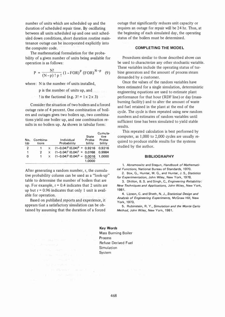
Consider the situation of two boilers and a forced outage rate of 4 percent. One combination of boil­ers and outages gives two boilers up, two combina­tions yield one boiler up, and one combination re­sults in no boilers up. As shown in tabular form:

Cumula-State tive

No. Combina- Individual Proba- Proba-Up tions Probability bility bility

2 X ( 1 -0.04)' (0'.04)° = 0.921 6 0.921 6 2 X ( 1 -0.04)' (0.04)' = 0.0768 0.9984

0 X ( 1 -0.04)' (0.04)' = 0.001 6 1.0000

1 .0000

Mter generating a random number, r, the cumula­tive probability column can be used as a "look-up" table to determine the number of boilers that are up. For example, r = 0.4 indicates that 2 units are up but r = 0.96 indicates that only 1 unit is avail­able for operation.

Based on published reports and experience, it appears that a satisfactory simulation can be ob­tained by assuming that the duration of a forced

outage that Significantly reduces unit capacity or requires an outage for repair will be 24 hr. Thus, at the beginning of each simulated day, the operating status of the boilers must be determined.

COMPLETING THE MODEL

Procedures similar to those described above can be used to characterize any other stochastic variable. These variables include the operating status of tur­bine generators and the amount of process steam demanded by a customer.

Once the values of the random variables have been estimated for a single simulation, deterministic engineering equations are used to estimate plant performance for that hour (RDF line) or day (mass­burning facility) and to alter the amount of waste and fuel retained in the plant at the end of the cycle. The cycle is then repeated using new random numbers and estimates of random variables until sufficient time has been simulated to yield stable results.

This repeated calculation is best performed by computer, as 1,000 to 2,000 cycles are usually re­quired to produce stable results for the systems studied by the author.

BI BLiOG RAPHY

1. Abramowitz and Stegun, Handbook of Mathemati­

cal Functions, National Bureau of Standards, 1970. .2. Box, G., Hunter, W. G., and Hunter, J. S., Statistics

for Experimentation, John Wiley, New York, 1 978. 3. Dhillon, B. S. and Singh, C., Engineering Reliability:

New Techniques and Applications, John Wiley, New York, 1 98 1 .

4. Lipson, C. and Sheth, N. J., Statistical Design and

Analysis of Engineering Experiments, McGraw Hill, New york,1 973.

5. Rubinstein, R. Y., Simulation and the Monte Carlo

Method, John Wiley, New York, 1 98 1 .

Key Words Mass Burning Boi)er Process Refuse Derived Fuel Simulation System

468