2WB05 SimulationLecture 4: DiscreteSimulation

Marko Boonhttp://www.win.tue.nl/courses/2WB05

November 26, 2012

2/17

Department of Mathematics and Computer Science

• Continuous systemsState changes continuously in time (e.g., in chemical applications)

• Discrete systemsState is observed at fixed regular time points (e.g., periodic review inventory system)

• Discrete-event systemsThe system is completely determined by random event times t1, t2, . . . and by the changes in state takingplace at these moments (e.g., production line, queueing system)

Writing a simulation

3/17

Department of Mathematics and Computer Science

Time advance:

• Look at regular time points 0,1, 21, . . . (synchronous simulation); in continuous systems it may be neces-sary to take1 very small

• Jump from one event to the next and describe the changes in state at these moments (asynchronoussimulation)

We will concentrate on asynchronous simulation of discrete-event systems

Writing a simulation

4/17

Department of Mathematics and Computer Science

Terms often used:

• SystemCollection of objects interacting through time (e.g. production system)

• ModelMathematical representation of a system (e.g., queueing or fluid model)

• EntityAn object in a system (e.g., jobs, machines)

• AttributeProperty of an entity (e.g., arrival time of a job)

• Linked listCollection of records chained together

Writing a simulation

5/17

Department of Mathematics and Computer Science

• EventChange in state of a system

• Event noticeRecord describing when event takes place

• ProcessCollection of events ordered in time

• Future-event setLinked list of event notices ordered by time (FES)

• Timing routineProcedure maintaining FES and advancing simulated time

Writing a simulation

6/17

Department of Mathematics and Computer Science

Basic approaches for constructing a discrete-event simulation model:

• Event-scheduling approachFocuses on events, i.e., the moments in time when state changes occur

• Process-interaction approachFocuses on processes, i.e., the flow of each entity through the system

In general-purpose languages one mostly uses the event-scheduling approach; simulation languages (e.g., χ )use the process-interaction approach

Writing a simulation

7/17

Department of Mathematics and Computer Science

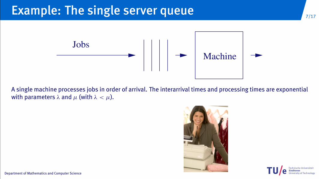
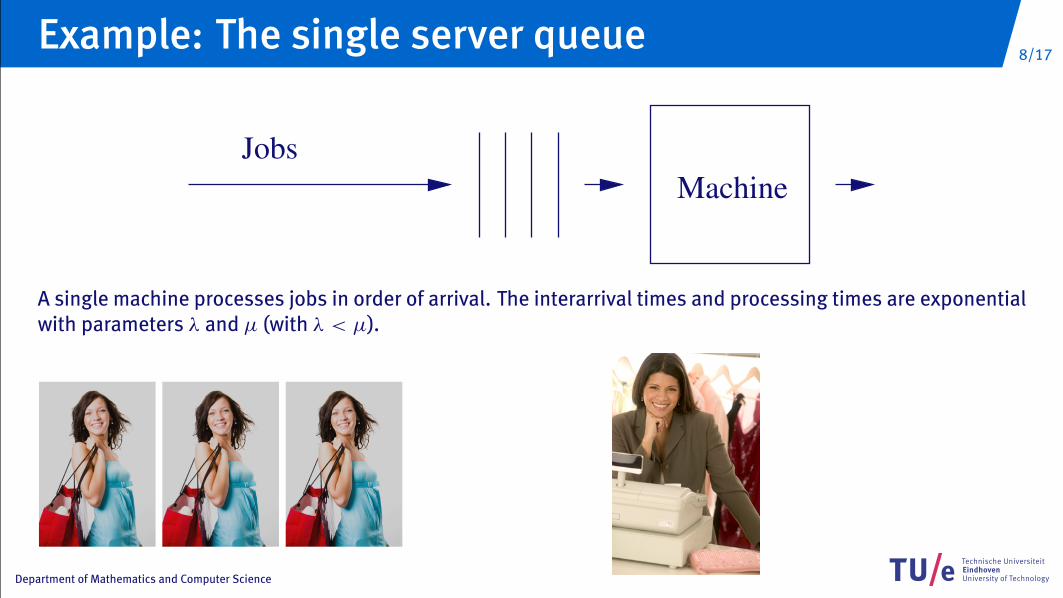
MachineJobs

A single machine processes jobs in order of arrival. The interarrival times and processing times are exponentialwith parameters λ and µ (with λ < µ).

Example: The single server queue

8/17

Department of Mathematics and Computer Science

MachineJobs

A single machine processes jobs in order of arrival. The interarrival times and processing times are exponentialwith parameters λ and µ (with λ < µ).

Example: The single server queue

9/17

Department of Mathematics and Computer Science

Relevant questions• What is the mean waiting time?

• What is the mean queue length?

• What is the mean length of a busy period?

• How does the performance change if we speed up the machine?

Example: The single server queue

10/17

Department of Mathematics and Computer Science

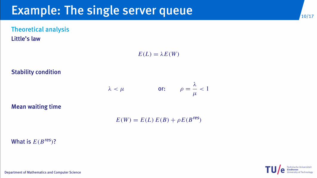
Theoretical analysisLittle’s law

E(L) = λE(W )

Stability condition

λ < µ or: ρ =λ

µ< 1

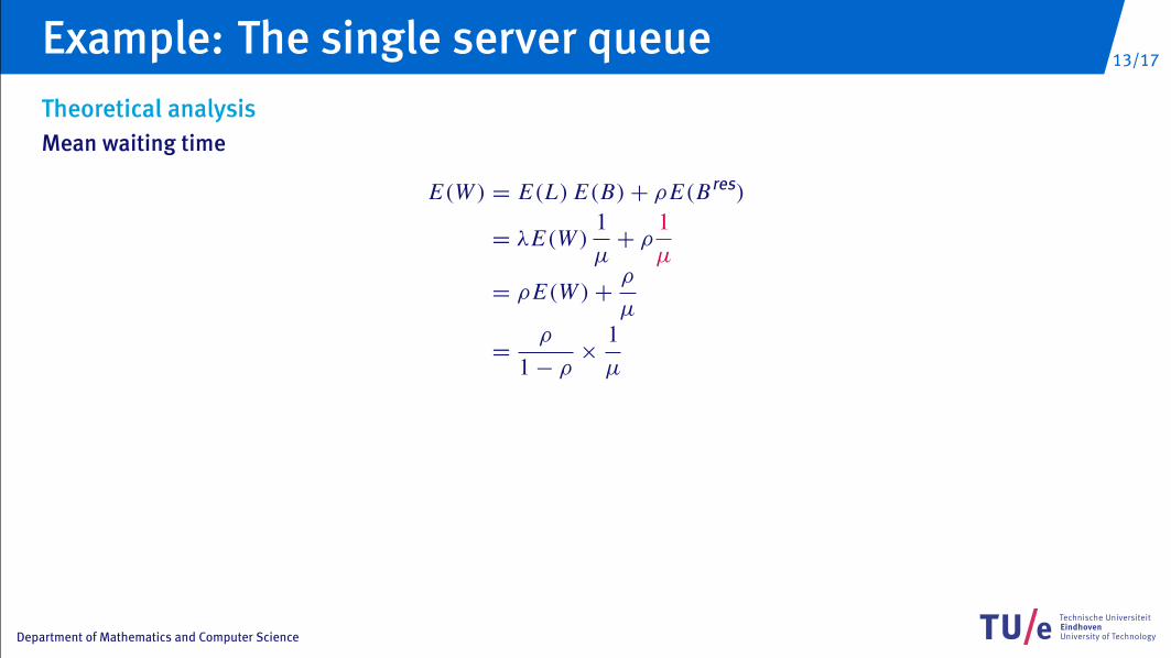
Mean waiting time

E(W ) = E(L) E(B)+ ρE(Bres)

What is E(Bres)?

Example: The single server queue

11/17

Department of Mathematics and Computer Science

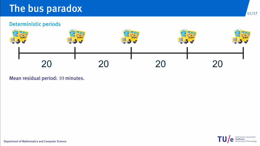
Deterministic periods

20 20 20 20

Mean residual period: 10 minutes.

The bus paradox

12/17

Department of Mathematics and Computer Science

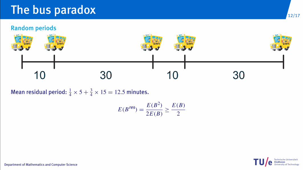
Random periods

10 30 10 30

Mean residual period: 14 × 5+ 3

4 × 15 = 12.5 minutes.

E(Bres) =E(B2)

2E(B)≥

E(B)2

The bus paradox

13/17

Department of Mathematics and Computer Science

Theoretical analysisMean waiting time

E(W ) = E(L) E(B)+ ρE(Bres)

= λE(W )1µ+ ρ

1µ

= ρE(W )+ρ

µ

=ρ

1− ρ×

1µ

Example: The single server queue

14/17

Department of Mathematics and Computer Science

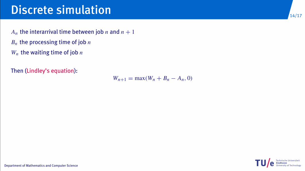
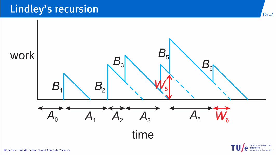
An the interarrival time between job n and n + 1

Bn the processing time of job n

Wn the waiting time of job n

Then (Lindley’s equation):Wn+1 = max(Wn + Bn − An, 0)

Discrete simulation

15/17

Department of Mathematics and Computer Science

time

work

A0

B1

A1

B2

A2

A3

B3 B

6

B5

A5

time

work

A0

B1

A1

B2

A2

A3

B3 B

6

B5

A5

time

work

A0

B1

A1

B2

A2

A3

B3 B

6

W6

W5

B5

A5

time

work

A0

B1

A1

B2

A2

A3

B3 B

6

W5

B5

A5 W

6

A5 +W6 = W5 + B5

Lindley’s recursion

16/17

Department of Mathematics and Computer Science

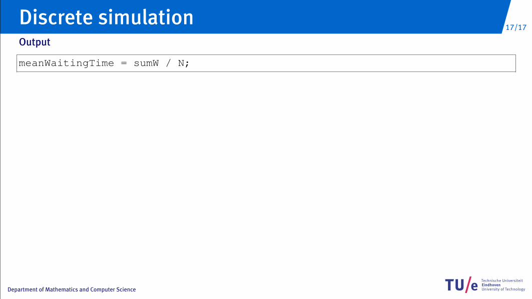
Initialization

int n = 0; //job numberdouble w = 0.0; // waiting time of job n// we assume that initially the system is empty

double sumW = 0.0; // sum of the waiting times

Main program

while (n < N) {double a = exponential(lambda);double b = exponential(mu);w = Math.max(w + b - a, 0);sumW = sumW + w;n++;

}

Discrete simulation

17/17

Department of Mathematics and Computer Science

Output

meanWaitingTime = sumW / N;

Discrete simulation