SIMULATION OF DEVELOPED RESIST PROFILEB FOR …

SIMULATION OF DEVELOPED RESIST PROFILEB

FOR ELECTRON-BEAM LITHOGRAPHY

by

Michael G. Rosenfield

Memorandum No. UCB/ERL M81/40

SAMPLE Report No. SAMD-6

12 June 1981

SIMULATION OF DEVELOPED RESIST PROFILES

FOR ELECTRON-BEAM LITHOGRAPHY

bY

M i chael G. Rosenf i e l d

Memorandum No, UCB/ERL M81/40

12 June 1981

ELECTRONICS RESEARCH LABORATORY

C o l l ege o f Engineer ing U n i v e r s i t y of C a l i f o r n i a , Berkeley

94720

SIMULATION OF DEVELOPED RESIST PROFILES FOR ELECTRON-BEAM LITHOGRAPHY

Michael G. Rosenf ield

Department of Electrical Engineering and Computer Sciences and the Electronics Research Laboratory

University o f California, Berkeley, California, 94720

ABSTRACT

A prog~~am for the simulation o f the time evolution o f two dimensional electron-beam exposed resist profiles is presented. The implementation o f an electron-beam machine in the user oriented computer program for the Simulation and Modeling 0.F Profiles in Lithography and Etching {SAMPL-E) i s discussed. Complete software documentation as well as a study of new electron-beam writing strategies and resist development effects are included.

Acknowledgements

I would first like to thank my research advisor, Pro- fessor Andrew R. Neureuther, for first suggesting the interface of an electron-beam simulation program with SAM- PLE. His guidance, support, and patience over the last two years were o f immeasurable help and made even the difficult times seem easy. I would also like to thank Professor Wil- liam G. Oldham f o r his support, advice, and f o r taking the time to talk with me that day in the Spring o f 1979 before I came to Berkeley.

Special thanks also must go to my colleagues in the SAMPLE group - especially to Sharad N. Nandgaonkar f o r the countless times I asked him for advice and help. Thanks are also to be extended to John L. Reynolds and Dr. Michael M. O'Toole for their suggestions. I would also like to thank Dr . Y. C. Lin for his advice. I am grateful to Dr. Ilesanmi Adesida and Or. David F. Kyser for their Monte Carlo calculations w h i c h make electron-beam simulation possible. I would also like to thank Dr. Chiu H. Ting for his help in the preparation of the publication in Appendix 11. The expert drafting b g Thomas King is also greatly appreci- ated.

Finally, I want to thank my family and friends (especially those 'back east') f o r their support and their faith in me.

Research sponsored b y the National Science Foundation Grant Eng77-14660 and an IBM Graduate Fellowship.

- 1. Introduction

As critical feature sizes in integrated circuits decrease, the importance o f electron-beam lithography (EBL) as an advanced processing technique has increased. Due to limitations in optical lithographic processes, electron-beam machines are currently being used in the production o f experimental devices and circuits with micron and sub-micron minimum dimensions C1-43 a s well a s in the manufacture of masks for optical and X-ray lithographic processes CS-63. The simulation o f the time evolution of two dimensional electron-beam exposed resist profiles is a very useful tool in the understanding and exploration o f electron-beam lithography for such applications.

This report deals with the implementation o f an electron-beam machine in the user oriented computer program for the Simulation and Modeling of Profiles in Lithogtaphy and Etching (SAMPLE) developed at the University of Califor- nia, Berkeley C7-103. As an example of the insight which can be gained using simulation, new electron-beam writing strategies and resist development effects are also discussed in an appendix.

Section I 1 deals with the EBL field in general and the important models used in the simulation. Section I 1 1 is a detailed explanation of the algorithms and program code. Appendix I is a User's Guide for the SAMPLE e-beam machine. Appendix I 1 is the manuscript o f a paper in which the e-beam machine is applied to a comparison of various electron-beam exposure strategies as well as an investigation into the actual resist development model used in the simulation. Appendix I 1 1 contains Common Block documentation and Appen- d i x IV contains the program code.

- 2 -

3. Electron-Beam LithoctraPhq a n d Simulation Models

In order to achieve h i g h resolution, EBL utilizes h i g h energy (10-50 Kev) electron-beam exposure of polymeric resists in place of more conventional wavelength limited UV and deep UV optical techniques. The loss of energy b y the electrons being scattered can affect the resist material in one of two ways: Generally, in negative resist, polymers are crosslinked making the resist insoluble in areas exposed to the beam. In positive resist, such as polymethyl- methacrylate ( P M M A ) , various mechanisms, such as depolymeri- zation, make the resist soluble in areas exposed to the beam. Thus, the rate of development of a resist is a function of the energy absorbed b y the resist C 1 1 1 .

In contrast to optical lithography, where an entire wafer or c h i p is exposed at once through a mask o f the desired exposure pattern, e-beam systems must perform the desired exposure b y serial data flow, i.e. writing out the complete pattern on the resist coated wafer. The two techniques for writing the pattern are vector scan and raster scan CS,61. In raster scan, the beam or wafer holding table is moved through a regular pattern with the beam being blanked off where no exposure is desired. In vector scanr the beam is onlq positioned in areas where exposure is I- equ ired.

The two most widely used types of beam used in e-beam systems are the Gaussian round beam and rectangular shaped beam C12-141. The advantage of rectangular shaped beams is increased throughput as a larger part o f the desired pattern is exposed at once C121.

In order to simulate the e-beam exposure and development processe5/ the absorbed energy density in the resist f o r a given exposure pattern must be known. Of the various methods bcj which the absorbed energy density can be determined C15-171, data from Monte Carlo ( M / C ) calculations C171181 is used in the SAMPLE e-beam program. The M/C technique is based on simulating a large number of individual electron trajectories to calculate the spatial distribution of energy deposited in the resist t191. A single scattering approach C171 is used where electrons from an idealized delta function electron-beam are elastically scattered b y the atomic nuclei in the target (resist film and substrate material for example) with the angle of scattering being chosen in a random manner. In between these elastic scattering events, the electrons travel a distance of one mean free path and are assumed to lose energy continuously ( i.e. linearly with path distance) due to inelastic scattering. This inelastic scattering is assumed to have negligi- ble effect on the trajectory of the electron C201. This is known as the continuous slowing down approximation ( C S D A ) . I t should be noted that although there are other M/C methods

- 3 -

which take into account other more exotic inelastic scattering events, such as core electron and plasmon excitation C l € 3 , 2 1 1 1 the CSDA approach has been found to give adequate results for type of data used in simulating EBL Cl81.

The M / C data used in the SAMPLE e-beam program is a two dimensional array of the energy absorbed in the resist b y a delta function line source. For a line source, the M/C computer program calculates the absorbed energy density at points in a plane in the resist perpendicular to the infin- ite line source. The plane is made up of two dimensional cells and the energy absorbed in each cell is output as the two dimensional array used in the SAMPLE e-beam program C171. This data is valid only for the resist material and underlying substrate(s) used in the calculations. Different resist-substrate combinations yield different M/C energy absorption arrays.

F r o m the M / C model of electron-beam exposure of resist, it can be seen that the scattering of the electrons in the exposure of one area of resist can affect other areas. Electrons can be backscattered from the resist and substrate

small isolated areas develop out slower than larger areas. This is the well known proximity effect E221 and is the fun- damental limitation of the resolution of EBL since in close packed geometries, the exposure of one area inherently exposes nearby areas. it can be seen that M/C data, and thus the SAMPLE e-beam program, implicitly simulates the proximity effect since the output array includes the energy density absorbed 2.5 to 5 um away from the incident delta function line source C17,1€31 .

and rexpose the same area as well as nearby areas. Thus,

Superposition is assumed to be valid. The absorbed energy density in the resist due to a delta function line source (i.e. the M / C data) can be convolved with the actual electron-beam exposure pattern to yield a two dimensional array which describes the absorbed energy density in a cross-section o f resist. Knowing that the rate o f development is a -Function of the absorbed ener'gy density, the time evolution of two dimensional resist profiles can then be generated.

Early models assumed that development occured along equi-energy contours in the resist C17,391. However, this assumption was found to be inadaquate C11,17,39,401 and the present model assumes that development is a surface etching phenomenon with t h e local etch rate determined b y the energy absorbed in the resist being removed C 1 9 1 .

Using the present model, the resist can be developed using various etching algorithms. Both a cell removal model C23!241 and the string development model C231 are currently used. In the cell model, the resist is broken u p into two

- 4 -

dimensional cells similar to those in the M/C calculations. The rate of dissolution of the resist in each cell that is in contact with the developer is determined b y an etch rate previously assigned to that cell. The rate of dissolution o f a cell depends on the etch rate as well as the number of sides exposed to the developer and whether or not these sides are adjacent E231.

The SAMPLE program uses the string model of development in w h i c h a string of straight line segments follows the developer-resist interface as a function of time C233. Dur- ing each development time step, each node (i.e. intersection of string segments) on the string is advanced at the local etch r a t e ( w h i c h is a function of the absorbed energy density at that point) in the direction o f the perpendicular bisector of the angle between adjacent segments. Segments are periodically added and deleted on the basis of length, and loops are deleted just prior ta profile output times c 1 9 1 . A more thorough explanation of the algorithms involved can be found in works b y Jewett and O'Toole C25,81.

Both development models have given adequate agreement with experimental profiles Ci9,26-281. The usefulness of simulation of EBC has been shown in a number of studies investigating proximity effects, resist materials, and writing strategies El?, 28-341. An example is contained in Appendix 11.

At present, all simulation studies have been done with the more widely used positive resists as an adequate model has not been developed for the development of negative resist. Most wovk to date, including this report, has been in the simulation of two dimensional cross-sections of resist profiles. Recentlyf Jones et a1 have reported a computer program which simulates resist development for EBL in three dimensions C351.

h

0- 00

I- d r w

U

x

\ \ \ \ \

\a < \ \ \ \

Figure 1. Symmetry o f t h e Monte C a r l o d a t a . The p r o g r a m u s e s t h e d a t a i n t h e l a t e r a l r a n g e .

- 5 -

3,. Propram Qperation a& Explanation of Code

The SAMPLE e-beam computer program consists of the following blocks o f subroutines, written in standard ANSI For- tran 77 (Appendix 4), which inputs user defined data, acts as a controller, computes the absorbed energy density array f o r the input exposure pattern, develops t h e resist, and prints out useful information and messages.

INPUT

Subroutines EXTRA6, TRL101, TRL102, TRLlO4, TRL105, TRL108, TRCllO, TRLlll, TRL112, TRL113, TRL114, and TRL115 are used to initialize default parameters (TRLlO1) and input user defined data w h i c h sets the exposure and developlment conditions needed f o r simulation. The use of 'Trial' statements or 'Key-words' to input data to the program b y way of these subroutines is discussed in Appendix 1.

CONTROLLER

Subroutine EBCTRL(numb) is the controlling subroutine which inputs the needed M/C data, initializes certain variables and directs other subroutines to form the expasure pattern, compute the absorbed energy density array, develop the exposed resist, and print out information.

CONVOLVER

Subroutines MLTSPT, EGAUSS, SQWGT, SPWGT, WEIGHT, MLTLIN(numb), BOUNDR, EARRAY, and function ERF(y) compute the overall exposure pattern and then convolve the M/C data under the pattern to give the final absorbed energy density array.

E-BEAM DEVELOPER

Subroutines EBDEV, ECYCLE, and function EBRATE(cz) along with subroutines LINEAR, CHKR, BNDARY, DELQQP(itype1, PLQTOUT, PLQTHP(ioutpt), and PRTPTS(iouptp1 from the SAMPLE program C81 develop the resist b y means of the string algorithm and print out the resultant resist profiles.

MESSAGES AND INFORMATION

Subroutines EBMSG(numb), PRARRY(numb), and DEVMSGtnumb) ( w h i c h is f r o m the SAMPLE program E811 print out pertinent information and error messages for the user.

GAUSSIAN ROUND BEAM

RECTANGULAR SHAPED BEAM

Figure 2. Simulated electron-beam shapes.

- 6 -

Common block documentation can be found in Appendix 111.

An explanation of the code and algorithms used is as f 01 1 ows: Clnce default values are initialized, and user defined data for the exposure pattern is input b y way of ‘Trial ’ statements or ‘Key-words’ (Appendix I)I subroutine EBCTRL(1) is called from subroutine TRL111. Information is read in from the file ‘mcdat‘ and the M/C data is stored in array EMAT(80,SOO). Oue to symmetry, all that is needed is the data from one side of the delta function line source (Figure 1). The M/C data is then multipied b y the ovelrall exposure dose and a constant to convert the data to units of J/cm**3. Variables are then initialized including the maximum number of array points which can be used in the arrays EMLT(1499) and ELIN(82,1002). This effectively limits the maximum distance between the first and last Gaussian shaped beams (spots) in a single line to 5 um and limits the ‘window‘ of resist which can be developed to 10 or 20 um depiend- ing on the M/C cell size in the horizontal ( x ) direction.

The SAMPLE e-beam program is capable of simulating Gaussian shaped o r rectangular electron-beams (Figure 2) C271. I f an exposure pattern is to be written with rectangular beams (each beam is considered one exposure line), subroutine SQWGT is called. SQWGT calculates the follawing expression which describes the rectangular beam profile c271:

erf [ (a-x)/ S IGMA*SQ2]+erf [ (a+x) / S I GLlA*SQZ] f(x) =

1 erf[ (a-x)/SIGMA*SQ2]+erf[ (a+x)/SIGMA*SQZ x=-w

where A=(l/2)FWHM (full width half maximum)l x is the distance frop the center of the bEaml SIGMA=edge width145 I

f l x ) corresponds to a location in the array ETEM2(999) with the distance between f(x) values set equal to the size of the M / C cell in the x direction (x=0 corresponds to ETEM2(nrhcet+l=ncemat).

and SQ2= J2 . Each normalized tg f(x) = 1 1 value of

It was found that when x equals 2a (i.e. fwhrn), f(x) is small (“OS and can be neglected. Thus, f(x) values need only be computed in this range. A warning is printed out if the fwhm of the beam is larger than the horizontal range o f the M/C data. Values for the error function are found using an anlytical expression E361 in function ERF which calculates:

x 2 erf(x) = - 1 e-t d t

4; 0

- 7 -

It should be noted that an overflow will result in function ERF i f the argument given to it is approximately greater than 12. In fact if the argument is greater than or equal to approximately 4, ERF will return a value o f 1. The right hand side, including the middle, o f the profile is stored in ETEM2 ( 5’95’ ) . Note that these ‘weights‘ which describe the beam are also multiplied b y the fwhm in order to assure that different sized beams with the same exposure dose develop out at approximately the same rate C373.

Subroutine EGAUSS is then called. In EGAUSS, the entire rectangular beam profile is entered into ETEM2(999) b y entering right hand side profile points in the corresponding opposite left hand side ETEM2(999) positions. This information is then transferred to array EMLT(l499) which contains the profile for an exposure line.

If the exposure pattern is to be written with lines composed of one or more Gaussian shaped beams, the rectangular beam algorithim in SQWGT is skipped. The standard deviation of the present spot being calculated is stored in DEVTEM while that 0 9 the previous spot is stored in DEUUNI. Similarly, the ‘weight‘ (see Appendix I ) is first stored in WGHTO until it is compared with the weight o f the previous 5 p O t I WGHTl . Subroutine SPWGT is called to calculate the profile for the Gaussian shaped beam. The beam is described b y the normalized Gaussian:

-x2 12 *S I G M A ~ e f(x) = f i * SIGNA

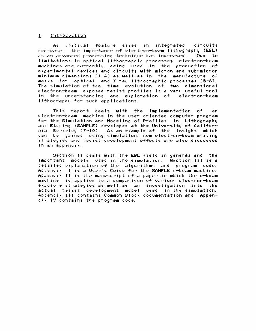
where SIGMA is the standard deviation. The total area under the beam is 1 and thus, each point in the beam profile for convolution can be described as a fraction o f the total area under the beam (Figure 3). The distance between each point describing the beam must be equal to the M / C cell sire in the x direction. The area under a Gaussian is:

x1 ) - erf(---) 2 1 kfi \zz e-x2/(2*SIGMA2) dx = erf(----- SIGMA X

S I GMA 1

m

where

erf(x) = -- dY 4zlT 0

and b y a change of variables, the error function can be re- writ ten:

/+-exposure spot

L

F i g u r e 3 . C o n v o l u t i o n o f a G a u s s i a n beam s h a p e . T h e s h a d e d a r e a i s t h e f r a c t i o n g i v e n t o t h e p o i n t a t x .

- 8 -

which is just 1/2 of the value returned from function ERF. Therefore, the profile for the Gaussian spot is calculated in SPWGT as:

1 x ' +CELLX/2 x'-CELLX/2)] * W('HT1 DEVTEM*SQ2 (DEVTEM*SQ2 F(x') = - [e r f ( 2

where CELLX is the horizontal M/C cell size, DEVTEM is the standard deviation, SQ2= Jz and WGHTl is the user defined weight for the spot. The middle of the spot (i.e. x=O) is located at ETEM2(ncemat). As with the rectangular beam, only the right hand side and middle of the Gaussian profile is calculated. 4 warning is printed out if the last array point of ETEMa(999) is not less than .0001, indicating that the standard deviation of the Gaussian is too large.

Upon returning from SPWGT, subroutine EGAUSS is called and the left hand side of the profile is calculated in the same manner as for a rectangular beam shape. The first spot profile in an exposure line is then entered into EMLT(1499).

If there is more than one spot per line, loop 408 is entered. The input distance between the present spot and the first spot (located at x=O.O) is changed from urn to units where 1 unit is equal to 1 M/C cell size in the x direction. This distance, ISHIFT, is rounded o f f to the nearest ce 11 . A check is made as to whether the distance between the present spot and x=O.O requires more array space than is available in EflLT(1499). If s o , an error message 15 printed and the program is stopped. The largest distance shifted is stored in ISLAR so that the actual number of array locations used in EflLT(1499) can be determined later in the program. If the standard deviation of the present spot is the same as the preceding, there is obviously no need to g a through subroutines SPWGHT and EGAUSS again. If only the user defined 'weights' are different, subroutine WEIGHT is called and ETEM2(999) is simply multiplied b y WGHTQ/WGHTl to calculate the profile. If the standard deviations are not equal, then subroutines SPWGT and EGAUSS are called and the new spot profile is stored in ETEM2(899). Subroutine MLTSPT then simply adds the new spot pattern to the previous pattern in EMLT(1499) with the new spot being offset from the first spot b y the ISHIFT distance. The entire loop is then completed and the next spot, if any, is calculated and added to the line. The overall process is illustrated in Figure 4.

Qnce the profile f o r the exposure lines are calculsted, the exposure profile in the user defined resist 'window of interest' 15 computed. This profile can be due to just one OT' up to twenty lines. The first line in an exposure pattern starts at x=O.O (i.e. the same location as the middle

c Q) L

t t 0 n 6

0 a v,

t

0 a v> c 0

3 0

0 0

0

\

+ h

W t

m

.-

L

w '-I-

W

w

F i g u r e 4. A d d i t i o n o f e x p o s u r e s p o t p a t t e r n s t o f o r m e x p o s u r e p a t t e r n ,

- 9 -

of the rectangular beam profile or the first Gaussian profile in a multiple spot line) and all other lines, if any, are referred to this point. FirstJ all line shifts are rounded to the nearest M/C cell and then restored in the array DISLIN(Z0). NUMCOL is the number of array locations of EMLT(1495’) which are used to contain the line pattern. If a symmetrical development (see Appendix I ) is requested b y the user, one-half o f the total number of array poinOs in the pattern, ITEMP, is computed. The variable SHIFT is the distance in um of the first spot or rectangular beam in the pattern from the left hand side resist window edge.

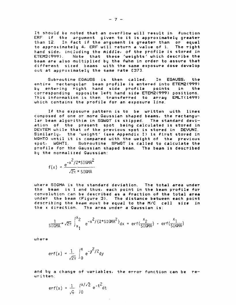
CPEDGE, used in the SAMPLE plotting routines, is set to It2 the size o f the window (CPWIND) in urn. ICPWIN is the number of columns in the final absorbed energy density array ELIN(82J1002) needed to develop the resist in the window. If this is too large, an error message is printed out and the program is stopped. NCLELU is the total numbdr of columns in ELIN(82,1002), including boundaries, which are required. The distance SHIFT is then set to either the symmetrical development SHIFT or a user defined SHIFT plus the distance in um of one cell size less than the range o f the M/C data in x (float(NRHCET)* CELLX-CELLX). This is because the total exposure pattern must be computed to + or - this extra distance from the window edges so that when the pattern is convolvedr all possible contributions from outside the window of interest are added in the window. Thus, when calculating the exposure profileJ the actual window size in array locations is (CPWIND/CELLX)+NCLMET (the number of array locations used in the ETEM2(999) array). Therafore the ’window’ for calculating the exposure profile, hereafter referred to as the ‘calculation window‘, is NCLMET larger than the ELIN(82J1002) window size as shown in Figure 5.

Subroutine MLTLIN(numb) calculates the input exposure pattern. I f the first spot or rectangular beam in the pattern is to the right of the left calculation window edge, MLTLIN(1) is called. MAX is the number of locations in array ELNWGT(1999) which make u p the calculation window. IPASSJ DIPASS, and TSHIF are variables used in conjunction with MLTLIN(2!). Loop 9 runs through each exposure line (starting with the first if MLTLIN(2) has not been calked). ISTAR and ITEM define the array locations in EMLT(1499) which will be added to a corresponding location in ELNWGT(1999). If a line is so far to the right of the calculation window that there is no possibility of contributing exposure in the window, a warning is printed out to the user indicating that line and all lines which follow do not contribute ( A return is then made to EBCTRL(1)).

Loop 20 adds the contribution for each line in the calculation window. It starts at the array location corresponding to the left hand edge of the winidow, ELNWGT ( 1 ) . 4 check is first made on ITEM. If ITdM is

i

L

3 0 73 c .- 3

F i g u r e 5 . I l l u s t r a t i o n o f t h e d i f f e r e n c e b e t w e e n t h e u s e r - d e f i n e d window a n d c a l c u l a t i o n window

- 10 -

negative, this means that the first contribution to the calculation window will be to the right of the present ELNWGT(j) location and both the ITEM and ELNWGT(j) locations are then increased b y 1. If ITEM becomes greater than the number o f array locations used in EMLT(1499), there is no further contribution from that line and the next line is calculated. Otherwise, the contribution from EMLT(item) multiplied b y the weight of that line, WGTLIN(k) (see Appen- d i x I), is added to ELNWGT(j).

MLTLIN(2) is called when the first spot or rectangular beam is to the left of the left calculation window edge. ITEST and ITTEST correspond to variables I S T A R and ISTEM in MLTLIN(1). If a line is too far to the left of the calculation window to contribute any exposure, a warning is printed out and the next line is calculated. If the beginning of a line (i.e. the location of the first spot or middle o f a rectangular beam) lies to the right of the left hand calculation window edge, that line (specified b y IPASS) and all others following it are added using MLTLIN(1). TSHIF contains the new value for the shift, i.e. the distance from the left hand window edge, and DIPASS is used so that MLTLIN(1) sees the correct distance between lines (DISLIN(k) contains the distance between line 'k' and the first exposure line. DISLIN(k)-DIPASS is the distance between line 'k' and the first exposure line to the right of the left calculation window edge). Otherwise, loop 120 adds the contribution to ELNWGT(j) in a manner similar to that of MLTLIN(1). I f ITTEST becomes greater than the number of array locations used in EMLT(1499), calculations for that line are completed and the next line is calculated.

The result of calling subroutine MLTLIN(numb) is a profile describing the exposure pattern as shown in Figure 5. The M/C data for a delta function line source can then be convolved under that profile to give the absorbed energy densitq in the resist window of interest.

Subroutine EARRAY is then called from EBCTRL(1) to per- f o r m the convolution. MAXCOL is the number of columns, excluding boundary columnsr which are used in ELIN(82,1002) to describe the absorbed energy density in the windbw of interest. Each row of M/C data and therefore each row of ELIN(82,1002) corresponds to a depth in the resist with the distance between 'depths' equal to the M/C cell size in the z or vertical direction. Also, each row of the M/C data has values for the absorbed energy density which are symmetrical about the delta function line source as explained earlier a n d shown in Figure 6. The exposure pattern is convolved b y constructing the exposure profile out of delta func%ions seperated b y a distance equal to 1 M/C cell size in the x direction as illustrated in Figure 7. Each r o w o f ELIN182,1002) 15 computed b y adding the contribution of absorbed energy density from each of the delta functiohs in

&LINE SOURCE

D C B A A B C D 1 . - - - - - e - - .

I 1 I '

I I -I -CELL X

ORIGIN

F i g u r e 6 . I l l u s t r a t i o n o f the symmet ry of t h e M/C d a t a . ' A ' , 'B', etc. a r e v a l u e s o f a b s o r b e d e n e r q y density i n a cell.

0 0 in 0 I

3

c

USER-DEFINED WINDOW

E LN W GT ( 2 4)

ELI N ( i ,2- 12) I (NCEMAT= 7)

- 1 1 -

the window of interest. The convolution is complete when the procedure has been carried out for each row of the M/C data.

Contributions from the left and left edge o f the window are first calculated. IMARK is the first array location of ELNWGT(1999) which contains a non-zero value. I f no non- zero values are found, this section of EARRAY is skipped. Assuming a non-zero value is located, loops 99, 199, and 299 add the contribution from the delta functions to the left of the window, including the edge, in the window with each row being done seperately (loop 99). Loop 199 sets the cocrect location of the delta function (i.e the ELNWGT(1999) array location) and the corresponding location, ITEM, in the M I C array EMAT(999) at which loop 299 starts. Loop 299 performs the actual convolution addition b y adding to each ELIN(i+lJl+lf column, starting at 1=1, the aborbed energy density due to a delta function located at ELNWGT(j1. The ‘+1‘ in the subscripts of the ELIN(82,1002) array allow for the addition of boundary rows and columns later in the p r o - gram. If the contribution from delta function, J I goes past the right window edge, J is incremented and the next delta function is calculated.

Contributions from the right and right hand edge of the window are then calculated. Again, IMARK is the first location in ELNWGT(1999), starting from the right, which contains the first non-zero value. As before, if there are no contributions, this section of EARRAY is skipped. ITCOL is equal to the number o f array locations used in ECNWGT(L999) plus one. L o o p s 399, 4991 and 599 add the contributions from the right o f the window in the window. Again, each row is done one at a time (loop 399). Loop 499 sets the parameters which determine the correct location of the delta function, i . e. ELNWGT(1999) position (J), and the corresponding location in the M/C array EMAT(80,500), ITEM, at which loop 599 starts. Loop 599 performs the convolution starting with the right-most delta function located at ELNWCT(itco1- imark). The contributions to ELIh!(l+l,l+l), starting at column MAXCOL+l and working left, from each delta function at ELNWGT(itco1-j) are calculated. The next delta function is calculated when the distance from the delta function to t h e ELIN(82,1002) location is greater than the range o f the M i C data (NCEMAT) o r when the contribution goes past the left hand window edge.

The convolution is then performed in the window of interest. This differs from the previous two cases in that contributions from both sides of the delta functions must be included. ISTART is the left-most ELNWGT(1999) location inside the window and IEND is the right-most location inside the window. Loops 201 and 202 control the convolution with each row again being done one at a time (loop 201). For e a c h delta function at location ELNWGT(j), contributions

- 12 -

from the left and then the right are added in the window. A location is skipped if ELNWGT(j)=O.

ILFCON is the number of ELIN(82,1002) columns to the left of the delta function. In loop 204, the contributions from the left of a delta function at ELNWGT(j) are added to ELIN(i+lf k + l ) starting with ELIN(i+lf2). I X is the corresponding location in EMAT(80,500). If I X is grceater than the M/C range, it is decreased while the ELIN(82t1002) column is increased until it is in range.

Loop 205 adds the contribution to the right of the delta function located at ELNWGT(j). I X is again the correct EMAT(8Qr500) location to use. ISCON is the first column in ELIN(82,1002) to the right of the delta function. Contributions are added in the window starting at ELIN(i+l,iscon) and continuing until past the right window edge or the range of the M/C data.

T h u s , at the end of EBCTRL(l), ELIN(82,1002) contains the absorbed energy density, due to an electron-beam exposure pattern, in a user defined window of resist. The resist is developed when EBCTRL(2) is called from subroutine TRL114.

Subroutine BOWNDR, called from EBCTRL(2)) simply adds boundary rows and columns to the previously calculated ELIN[82,1002) array. The code is similar to that used in subroutine CLCMXZ in SAMPLE C83. Boundary values are found b y linear extrapolation with extrapolated values less than 0.0 set to 0.0. The boundaries are required in the development routines. Upon return from BOUNDR, parameters needed in the SAMPLE development algorithms are initialized.

The develop subroutines listed in Appendix IV are very similar to the SAMPLE optical develop routines explained in Mike O'Toole's Ph.D. thesis E81 and therefore only a brief explanation will be given. The development controller, subroutine EBDEV, is identical to subroutine DVELOP in SAMPLE C 8 3 except that when estimating the time until developer breakthrough to the substrate, the maximum value of absorbed energy density in the top row (not including boundaries) of ELINI82, 1002) is found. This is because the rate of development increases with increasing energy density. There is also a slight difference when calculating the variable MAXPTS Ii.e. a divison b y the window size in um).

Function EBRATEIcz) is the same as function RATE(cz) C81 except that the rate equation (and background rater BACRAT) applicable t o EBL is used C 1 9 1 :

ALPH R(D) = R l ( c +")

Do

- 13 -

!See Appendix I )

Subroutine ECYCLE is the same as subroutine CYCLE t81 except that an anisotropic development feature C28~ see Appendix I 1 1 is incorporated. The user mag input the fraction o f horizontal development desiredJ FRACi with the default value being, o f courser 1.0. The string point XE(m) is then advanced the normal length in the z direction; but) onlq F R A C o f the normal length in the x direction.

The rest o f the development subroutines come from the SAMPLE program E 8 1 as explained earlier.

Subroutine EBMSG(numb1 prints out various types o f information and messages if called from other subroutine6 in the SAMPLE e-beam program. Subroutine PRARRY(numb1 prints out the various arrays used in the program if instructed to do so b y the user (See Appendix 1). Subroutine EPLOT prints out desired rows of ELIN(82,1002) into a file 'engpts' which can be plotted to give energy density distribution profiles for various depths in the resist (See Appendix I). The remainder o f the code (the INPUT subroutines listed earlier) are the 'Trial' subroutines used to input exposure and development conditions to the program.

- 14 -

References

e 1 1

c21

c31

e43

e51

C61

e71

C 8 1

c 9 1

J.R. Toker, M.R. Oliverr A.P. Lane, and R.H. Havemdnn, "Fabrication and characterization of e-beam defined mosfets with submicrometer gate lengths", 1980 IEDM Technical Digest, p p . 768-771, December 1980.

R.K. Watts, W . Fichtner, E.N. Fulsr R.L. Johnston, and L.R. Thibault, "Electron beam lithography f o r small mosfets", 1980 IEDM Technical Digest, p p . 772-775.

Y . Sakakibara, T. Ogawa, K. Komatsu, S. Moniya, M. Kobayashi, and T. Kobayashi, "Electron-beam direct writing technology for lum VLSI fabrication", 1980 IEDM Technical Digest, p p . 425-428.

S. A. Evans, S. A. Morris, L. A. Arledge, Jr. I J. 0. Englade, and C.R. Fullerl " A 1-urn bipolar VLSI technol- ogyl'I IEEE Trans. Electron Devices, vol. ED-27, pp . 1373-13781 1980.

J.A. Dohertry, "Recent advances in electron beam systems for mask making", Solid State Tech., vol. 221 no. SI p p . 83-88, 1979.

J. A. Reynolds, "An overview of e-beam mask-making", Solid State Tech. vol. 22, no. 8 1 p p. 87-94, 1979.

S.N. Nandgaonkar, "Design of a simulator program (SAM- PLE) for IC fabrication", M.S. Report, Department of Electrical Engineering and Computer Sciences, U. C. Berkeley, 1978.

M. M. O'Toole, "Simulation of optically formed images in positive photoresist", Ph. D. Thesis, Department of Electrical Engineering and Computer Sciences, U.C., Berkeley, 1979.

W. G. Oldham, S. N. Nandgaonkar, A. R. Neureutherl and M. M. O'Toole, "A general simulator for VLSI lithography and etching processes: Part I -- application to ,projection lithography", IEEE Trans. Electron Devices, vol. ED-26, no. 4, p p . 717-722, 1979.

C 1 0 1 W.G. Oldham, A.R. Neureuther, C. Sung, J.L. Reynolds, and S.N. Nandgaonkar, " A general simulator for YLSI lithography and etching processes: Part I 1 -- application to deposition and etching", IEEE Trans. Electron Devices, vol. ED-27, no. 8, pp. 1455-1459, 1980.

e111 M. Hatzakis, C.H. Ting, and N. Viswanathan, "Fundamen- tal aspects of electron beam exposure of polymlsric resist system", Proc. 6th Int. Conf. on Electron and Ion Beam Sci. and Tech. (Electrochemical Society), pp .

- 15 -

542-3790 1974.

C121 H. C. Pfeiffer, "Recent advances in electron-beam lithography for the high-volume production o f VLSI devices", IEEE Trans. Electron Devices, vol. ED-26, no. 4, pp. 663-6741 1979.

ti31 E.V. Weber and R.D. Moore, "E-beam exposure for sem- iconductor device lithography", Solid State Tech. I v o l . 22, no. S f pp. 61-67, 1979.

Cl41 H . C . Pfieffer and G.O. Langner, "Advanced beam shaping techniques for electron lithography", Proc. 8th Int. Conf. on Electron and Ion Beam Sci. and Tech. (E'lec- trochemical Society), p p . 149-159, 1978.

C1Sl J .S . Greeneich and T. Van Duzer, "An exposure model for electron sensitive resist", IEEE Trans. Electron Dev- ices, vol. ED-21, no. 5 , pp. 286-299, 1974.

ti63 R. J. Hawryluk, A.M. Hawryluk, and H. I. Smith, "Energy dissipation in a thin polymer film b y electron beam scattering", J. Appl. Phys., vol. 45, no. 61 p p . 2551- 2546, 1974.

t i71 D.F. Kyser and K. Murata, "Monte Carlo simulation of electron beam scattering and energy loss in thin films on thick Proc. 6th Int. Conf. on Electron and Ion Beam Sci. and Tech. (Electrochemical Society), pp. 205-2251 1974.

CIS1 I. Adesida, "Electron energy dissipation in layered med ia", Ph. D. Thesis, Department o f Electrical Engineering and Computer Sciences, U . C . , Berkeley, 1979.

Cl'irl A . R . Neureuther, D . F . Kyser, and C.H. Tingt "Electron- beam resist edge profile simulation", IEEE Trans. Elec- tron Devicesl vol. ED-26, no. 4, pp. 686-6931 1979.

E203 D.F. Kyser, "Monte Carlo Simulation in Analytical Elec- tron Microscopy", in 'Introduction to Analytical E,lec- tron Microscopy', J. I. Goldstein, J. Hren, D. C. J o y f ed., Plenum Press, 1979, chap. 6.

E211 R . Shimitu, Y. Kataoka, T. Ikuta, T. Koshikawa, and H. Hashimoto, " A Monte Carlo approach to the direct simulation of electron penetration in ~ o l i d s " ~ J. Phys. I): Appl. Phys. I V O ~ 9, pp. 101-114, 1976.

C221 T. H. P. Chang, "Proximity effect in electron-beam lithography", J. Vac. Sci. Tech. vol. 121 no. 61 p p . 1271-1275, 1975.

- 16 -

C231 R.E. Jewett, P. I. Hagouel, A.R. Neureuther, and T. Van Duzer, "Line-profile resist development simula'tion techniques", Polymer Eng. Sei.# vol. 141 no. 6, p p . 381-3841 1977.

C241 F.H. Dill, A.R. Neureuther, T.A. Tuttle, and E. J. Walker, "Modeling projection printing of positive photoresist", IEEE Trans. Electron Devices, vol. ED4-22, no. 71 pp. 456-444, 1975.

C253 R.E. Jewett, "A string model etching algorithm"l M.S. Report, Department of Electrical Engineering and Com- puter Sciences, U. C. I Berkeleyl 1979.

C241 K. Murata, E. Nomura, K. Nagami, T. Kato, and H. Nakata, "Experimental and theoretical study of cross- sectional profiles of resist patterns in electron-beam lithography", J. V a c . Sci. Tech., vol. 16, no. 61 pp. 1734-1738, 1979.

C271 D.F. Kyser and R. Pyle, "Computer simulation of electron-beam resist profiles", IBM J. Res. Develop. I

vol. 241 no. 4, p p . 426-437, 1980.

C283 M. G. Rosenf ield and A. R. Neureuther, "Exploration of electron-beam writing strategies and resist development effect^"^ P r o c . 9th Int. Conf. on Electron and Ion Beam Sci. and Tech. (Electrochemical Society), pp. 382-395, 1980.

C293 D.F. Kyser and C.H. Tingl "Voltage dependence of proximity effects in electron beam lithography", J. Vac. Sci. Tech. vol. 16, no. 6, pp. 1759-1763, 1979.

C301 J.S. Greeneich, "Impact o f electron scattering on linewidth control in electron beam lithography", J. V a c . S c i . Tech., vol. 161 no. 6, p p . 1749-17531 1979.

C 3 1 1 J . S . Creeneich, "Proximity effects in electron-beam exposure of multi-layer resists, P r o c . 9th Int. Conf. on Electron and Ion Beam Sci. and Tech. (Electrochemi- cal Society), pp. 282-303, 1980.

C321 Y. Todokoro, "Double-layer resist films for submicrometer electron-beam lithography", IEEE Trans. Electron Devices, vol. ED-27, no. 81 p p . 1443-1448, 1980.

C331 M. Nakase and M. Yoshimi, "Quantitative evaluation of proximity effect in raster-scan exposure system for electron-beam lithography", IEEE Trans. Electron Dev- ices, vol. ED-27, no. 8, pp . 1460-146,5, 1980.

- 17 -

C341 M.P.C. Watts, P. Rissman, and J. Kahn, "Solubility ratio, sensitivity and line profile control in positive e-beam resists", Proc. 9 t h Int. Conf. on Electron and Ion Beam in Sci. Tech. (Electrochemical Society), pp. 375-381 I 1980.

C351 F. Jones, J. Paraszczakr and M. Hatzakis, " A three dimensional model f o r resist development simulation", Proc. 9th Int. Conf. on Electron and Ion Beam Sci. and Tech. (Electrochemical Society), pp . 351-364, 1980.

C36l C. Hastings, Jr. I 'Approximations for Digital Comput- ers', Princeton, New Jersey: Princeton Univerisity Pressl 1955, p . 107.

C371 D. F. Kyser, private communication.

C381 Papoulis, 'Probability, Random Variablesl and Stochas- tic Processesrl New York: McGraw Hill, 19651 p p . 65-66.

C393 J.C.H. Phang and H. Ahmed, "Line profiles in thick electron resist layers and proximity effect correc- tionttl J. Vac. Sci. Tech. vol. 16, no. 6, p p . 1754- 17581 1979.

C401 J.S. Greeneichl "Time evolution of developed contours in PMMA electron resist", J. Appl. Phys., vol. 45, pp. 5264-52681 1974.

Appendix A -- USER'S GUIDE

SAMPLE E-BEAM USER'S GUIDE

Michael G. Rosenfield


University of California, Berkeley, California 94720

Version i. L Februarq z1 1981 Introduction

The SAMPLE (Simulation and Modeling of Profiles in Lithography and Etching) computer program, with the addition of an electron-beam machine, now has the capability to simulate the time evolution of two dimensional resist profiles f o r electron-beam lithography. Monte Carlo data, giving the spatial distribution of energy deposited in the resist b y a delta-function line sourcel is convolved with a pattern of arrayed Gaussian [spot) or rectangular shaped electron- beams. This gives the energy density absorbed in a 'window' of resist for various patterns of exposure. The development is then simulated using a simple etch-rate versus dose curve and SAMPLE'S string model of development. E-beam simulation can b e implemented in SAMPLE through a series of 'trial' statements (as is done presently) or b y their corresponding key-words for the general interface.

Overall Prooram Operation

Basicallyl the program is run b y the user in the following manner: Default values are first initialized. An exposure line is then set. This line may be a single rectangular beaml a single Gaussian beam, or a group of arrayed Gaussians. This line can then be arrayed to form an exposure pattern consisting of one or more lines. The part o f the exposed resistl relative to the exposed line patternl which is to be investigated (i.e. the 'window of interest') is set b y the user. The Monte Carlo data is then convolved with the exposure pattern in the window of interest at an overall exposure dose (uC/cm++2). The number of points in the development string, development times, and the constants for the development rate equation( the etch-rate as a function of absorbed energy density) are then inputted. The resist is then developed. The overall exposure dose can be changed without having to reconvolve the exposure pattern and another development can be run. Also, the various arrays used in the program as well as the energy a b s o r b k d at specified depths in the resist in the window of interest can b e printed out if desired.

- 2 -

g-Beam Trial and Tenative Keu-Word Summarq

TRIAL 101 -- EBLITH

Default Parameters

Trial 101 (no arguments) initializes the default parameters and must be run first for correct initialization.

TRIAL 102 -- EBLPRINT

Output Printing Flags

Trial 102 arg2 arg3 arg4 arg5 argb sets flags which control the outputting of the various arrays used in the e-beam program as well as information pertaining to the exposure and development conditions. If arg2-1, the one-dimensional arrays EMLT(1499) (which contains the exposure pattern for a single line) and ELNWGT(1999) (which contains the exposure pattern needed to compute the absorbed energy in the window of interest) are outputted. If arg3=1 the final two dimensional energy density arrayf ELIN(82,1002), is printed out row b y row (including boundaries). Note that ELIN(82,1002) will only be outputted if an actual development is requested. If arg4=lf the one dimensional array ETEM2(999) (which contains the exposure pattern for a single Gaussian or rectangular beam) is printed out. I f arg5=l, the array E M A T ( 8 O f 5 O 0 ) ( w h i c h contains the inputted Monte Carlo data multiplied b y the dose and in units of J/cm**3) is outputted. If argb=l, information pertaining to the exposure and development conditions is printed out.

TRIAL 104 -- EBLRATE

Etch-Rate Parameters

Trial 104 arg2 arg3 arg4 arg5 sets the development rate equation constants. The rate equation used is C l l :

ALPH R ( D) = R 1 ( Cm+D/Do)

where R(D) is the etch-rate in A / s e c f D is the absorbed energy density in J/cm**3, RlCm is the background etch- ratef Cm is a constant inversely proportional to the initial number average molecular weight, DO is a reference or knee energyf and ALPH is the asymptotic slope o f the etch-rate versus absorbed energy density curve at h i g h dose. Arg2 changes the default value of R1. Arg3 changes the default

- 3 -

value of Cm. Arg4 changes the default value of DO and arg5 changes the default value of ALPH.

TRIAL 105 -- EBLPATSQ

Rectangular Beam

Trial 105 arg2 arg3 sets the full-width half maximum (fwhm) value and edge-width if a rectangular shaped beam is desired. Arg2 sets the fwhm and arg3 sets the edge-width fi.e. the lateral distance between the 10% and 90% points o f the rectangular beam. An edge-width o f 0.0 is not allowed. Note that one rectangular beam is considered one exposure line in the program.

TRIAL 106 -- EBLPATPS

Periodically Arrayed Gaussian Beams

Trial 106 arg2 arg3 arg4 arg5 arg6 . . . . sets the exposure pattern for a line made u p of periodically arrayed, identical {same standard deviation) Gaussian beams (spots). Arg2 is the number of Gaussian beams in the line. Arg3 is the distance (negative numbers are not allowed) in microns between the center of the beams. Arg4 is the standard deviation of the spots. Arg5, arg6 and beyond are the 'weights' of each spot. ArgS specifies the weight of the first spot, Arg 6 specifies the weight of the second spot, and so on. Each spot must have a corresponding weight. The weights indicate how much of the overall exposure dose is given to each Gaussian beam. For example, if there are 10 spots in a 1 um line, then the weight o f each spot would be . l . The weights are very dependent on how the actual machine being simulated distributes the total dose of the electrons. Note that at least 2 spots must be specified to use trial 106. There is a maximum of 20 spots per line.

TRIAL 107 -- EBLPATNS

Non-Periodically Arrayed Gaussian Beams

Trial 107 arg2 arg3 arg4 arg5 . . . . . . sets the exposure pattern for a line made up of a non-periodic array of Gaus- sian beams. Each spot and its location relative to the first spot (which MUST be set at 0.0 microns) must be com- pleteley specified. A r g 2 is the number o f spots. Arg3 is the position of the first spot (0.0). Arg4 is the standard deviation o f the first spot. Arg5 is the weight o f the

- 4 -

first spot. Similarly, args6-8 would describe the second spot, etc. At present, the maximum a spot may be shifted from the first spot at 0.0 microns is 5.0 microns-this holds for trial 106 as well. Negative distances are not allowed and the maximum number o f spots per line is 20.

Note that trial 105 or trial 106 or trial 107 specifies an exposure line. Two or more o f these trials being used will result in the last trial called being the one which specifies the line. Also note that the convolution accuracy is limited b y the M/C cell size in the horizontal direction. Accuracy is degraded significantly when the standard deviation or edge-width is less than one M/C cell size in x.

TRIAL 108 -- EBLPLINE

Periodic Line Pattern

Trial 108 arg2 arg3 arg4 arg5 . . . . . . sets the exposure pattern for a series of periodically arrayed lines. A r g 2 is the number of lines (2 or more). Arg3 is the periodic distance (negative numbers not allowed) between the center of two adjacent rectangular beam lines or the distance between the centers o f the first spots in Gaussian beam lines. Arg4, arg5, etc. are the weights for each line. There must be one weight for each line. The weights allow the user to vary the relative overall exposure doses o f each line. The maximum number of lines is 20.

TRIAL 109 -- EBLNLINE

Non-Periodic Line Pattern

Trial 109 arg2 arg3 arg4 . . . . . . sets the exposure patterns for one or more non-periodically arrayed lines. Each line and its location relative to the first line (which MUST be 0.0 microns) must be specified. Arg2 is the number o f lines. A r g 3 is the position of the first line (0.0). Arg4 is the weight of the first line. Similarly, arg5 and argb specify the second line and so on. There is no limit to the distances between lines. Howeverr the Monte Carlo data only extends a finite distance. The program will warn the user when a line can not possibly contribute any energy density to the window o f interest. Negative distances are not allowed and the maximum number of lines is 20. Note that this trial can be used to construct patterns of lines with different linewidths. F o r example, two 1 um rectangular beams can be arrayed to overlap at the half-maximum point to form a 2 urn line.

- 5 -

TRIAL 1 1 0 -- EBLWIND

Window of Interest

Trial 110 arg2 arg3 arg4 sets the convolution and development window size and the position of the total exposure pattern in the window. Arg2 is the window size in microns. For Monte CaT.10 data with .02 um and less lateral cell size, the maximum size of the window is 10um. F o r cell size greater than . Q 2 um, the maximum window size is 2Qum. Note that the larger the window, the larger the CPU time to run the program. I f arg3=ll the left edge of the window will start at approximately (within one Monte Carlo cell size) the center o f the exposure pattern li.e. symmeerical development). If arg3=O, the position of the first spot in the first line or the position of the center of the first rectangular beam line in relation to the left window edge must be specified in arg4. I f the first spot or rectangular beam is to the right o f the left window edge, arg4 will be a positive number of microns. If to the left, arg4 will be negative.

TRIAL 1 1 1 -- EBLCNVLV

Convolution - Dose

Trial 1 1 1 arg2 runs the convolution and sets the overall exposure dose. Arg2 is the overall exposure dose in uC/cm**2. This overall dose is distributed over a line b y way of the weights of each Gaussian as was explained previously. In the case of a rectangular beam, each beam receives the overall dose.

TRIAL 112 -- EBLSTRPTS

String Points - Anisotropic Development

Trial 112 arg2 arg3 sets the number o f string points and the anisotropic development option. Arg2 is the number of points in the development string in the window of interest. 30-40 points/micron is usually sufficient. Accuracy and CPU

arg3 is set less than 1, there will be a reduction in the lateral motion of the string nodes b y a factor of (l-arg3) c21. I f arg3 is set greater than 1 or less than 0, tthere will be erroneous results.

time increase as the number of string points increases. If

TRIAL 113 -- EBLNEWDOSE

- 6 -

Change Dose

Trial 113 a r g 2 changes the overall dose of the final energy array without reconvolving the entire exposure again. Arg2 is the new dose in uC/cm**2. Usually, trial 113 would be r u n after a development to change the dose for a subsequent development.

DEVT I ME

Development Times

Devtime argl to arg2, arg3 sets the development times from argl to arg2 seconds in arg3 steps and is the same as used in the rest o f the SAMPLE program.

TRIAL 114 -- EBLDEVELOP

Development

Trial 114 (no arguments) runs the development.

TRIAL 115 -- EBLENGPTS

Absorbed Energy Density Contours

Trial 115 a1.92 arg3 arg4 sets the conditions for the printing out of various rows (depths) of the final energy array in the window of interest. If arg2=ll then the program will determine the maximum energy (ymax) printed in the output. I f arg2 is any other positive integer (J/cm**3), that value will be used as the maximum energy. This maximum energy is printed out before the actual energy points and is only used for plotting purposes. Arg3 is the first row o f the energy array to be printed out (l=top of the resist, # of rows of Monte Carlo data=bottom). Arg4 is the 'skip' number of rows-i.e. the number of rows added to the number o f the first row to determine which row will be printed out. For example, for Monte Carlo data o f 40 r o w s r arg3=1 and arg4=19 would result in rows 1,20,39 being printed out. This trial statement was inspired b y a similar option in IBM's Lithog- raphy Modeling System (LMS) C31.

TRIAL 2

Output Options

- 7 -

Trial 2 arg2 arg3 arg4 from SAMPLE sets various printing options. If arg2=1, extra diagnostic printout is produced b y the development machine. If arg3=lJ points are printed for the developed plot suitable for plotting b y HP graphics terminals or plotters at Berkeley. If arg4=lJ a slowerJ m o r e accurate algorithm is used which uses more string points and produces more accurate plots; little effect occurs for line printer plots.

_I The E-BEAM Prosram at. Berkeleq Presently, the E-BEAM-SAMPLE simulation program runs on

a VAX PDP 11/780 compiled with the Fortran f77 compiler. Line printer output includes a plot of the developed contours. Through the use of f77‘s ‘open‘ and ‘close‘ com- mandsJ points for plotting the final energy profiles (trial 115) and the developed resist profiles are printed out into files ‘engpts’ and ’f77punch7’ respectively.

Monte Carlo Data

At presentJ the €-Beam program does not have the capability to generate the Monte Carlo data needed f o r the simulation. As this requires large amounts of computer timeJ several Monte Carlo files C41 are supplied with the main program. This data is f o r PMMA resist coats of 1.5 and . 5 um on Si at 10 and 20 KeV beam energies. The cell size is .Ol um in x and . 1 um in z. The data is read from file ‘mcdat‘ in subroutine EBCTRL(numb) using ‘open‘ and ‘close‘ statements and has the following form:

resist thickness (urn) beam energy (KeV) number to convert Monte Carlo data to J / c m * * 3 cell size in the x (lateral) direction in microns cell size in the z (vertical) direction in microns number of rows of data (i2 formatJ maximum-80) number. of columns of data (i3 formatt maximum-500) Monte Carlo data-8e10.4 format per line. One entire row immediately following another.

Miscellaneous

F o r use on smaller computersJ the Monte Carlo (EMAT(80J500)) and final energy (ELIN(82J1002)) array sizes can be reduced. This is done b y changing the array sizes in the common blocks /CNVLV2/ and /LINEl/. Also, the checks for the input EMAT(8OJ500) size and the window size settings in subroutine EBCTRL(numb) must be changed. In subroutine EBMSG(numb), message 6 must also be corrected for the new maximum number o f columns in the EMAT(BO,500) array.

Different rate equations can be used b y changing the /RATDAT/ common block and the EBRATE (etch-rate) and BACRAT

- 8 -

(background etch-rate) expressions in function EBRATE(cz1. Note that the SAMPLE development routines require the etch- rate in units of umlsec.

Default Parameters-& in Trial 101 C 1 1 set printing flags so that only exposure and

development info. is printed

C21 rate curve data for PMMA 2010; 1 : 1 M1BK:IPA developer: Rl=l. 0 Cm=l. 0 DO= 199 ALPH=2. 0

C31 exposure pattern: 1.0 urn rectangular beam with .25 um edge-width 3 periodic lines, 2.0 um apart (center to center) dose=80 uC/cm**2

C41 development: symmetric with 2.0 urn window, 60 string points 40 to 160,4 development times

C51 energy plotting option first row=l s k i p rows-7 program sets ymax

C 6 1 print out points for plot

Examples of SAMPLE Inout Files for E-BEAM

The following input files are designed to illustrate the use of the e-beam simulation program in SAMPLE. The first input file is the simplest one possible:

**initialize default parameters trial 101 **run convolution trial 1 1 1 **print pts f o r energy contours trial 115 **develop trial 114 $

The above file simulates an exposure pattern made entirely from the default values previously discussed. Statements beginning with one or more '*' are regarded as comment lines b y SAMPLE. The '$ ' at the end of the file tells SAMPbE to perform the operations indicated b y t h e last trial statement and then stop as there is no more input. Figure 1 s h o w s t h e developed profiles as plotted on an HP 2648 graphics

0

0 1

0 0

- 9 -

terminal at Berkeley. Monte Carlo data for 1 . 5 um PMMA on Si at 20 KeV was used. Figure 2 shows a plot of the energy absorbed in the resist in the development window for rows 1,8, and 1 5 of the final energy array ( i . e. the top, middle, and bottom of the resist).

The next input file illustrates many more aspects o f the use of the various trial statements:

**initialize default parameters trial 101 **set flags trial 2 0 1 1 **specify line trial 1 0 5 1 . 5 . 3 **specify array of line(s) trial 1 0 9 1 ( Q 1) **specify convolution and development window trial 1 1 0 3 0 1 . 3 **set dose and run convolution trial 111 90 **set number of string points trial 1 1 2 60 **set development times devtime 10 to 90,9 **develop trial 1 1 4 * Trial 2 says to print out the developed profile points into the file 'f77punch7' and also to use a more exact development (for better plotted profiles from the HP graphics terminal). Trial 1 0 5 sets a rectangular beam to fwhm of 1 . 5 um and edge-width of . 3 urn. Trial 109 says to write only this one line with a weight o f 1 (note that parentheses are ignored b y SAMPLE and are only used for clarity). Trial 1 1 0 sets a 3.0 um window with the center o f the rectangular beam 1 . 5 um from the left edge of the window. Trial 1 1 1 runs the convolution with an overall exposure dose of 90 uC/cm**2. Trial 1 1 2 says to use 60 string points and devtime says to develop from 1 0 to 90 seconds in 1 0 second intervals. Fig- ure 3 shows the resulting profiles in . 5 um of PMMA on Si at 20 KeV. Default PMMA 2010 developed in 1:l M1BK:IPA is used as the resist.

The last two examples use Gaussian beams to form the exposure lines:

**initialire default parameters trial 1 0 1 **set flags trial 2 1 1 1 **spec if y 1 ine trial 107 4 (0 .05 .2) (.2 . 1 .2) (.4 . 1 .2) ( . 6 . 0 5 .2)

- 10 -

**specify array o f lines trial 108 2 1. 1 1 1 **specify convolution and development window trial 110 2.5 0 . 4 **set dose and run convolution trial 1 1 1 80 **set number of string points trial 112 100 **set development times devtime 10 to 50t5 **set rate equation constants trial 104 8.33 1.0 325 1.404 **deve 1 op trial 114 **change dose and do another development trial 113 40 trial 114 B

The first ‘ 1 ’ in trial 2 says to print extra diagnostic out- p u t with the developed profile. Trial 107 says to make up a line of 4 Gaussiansr spaced .2 um apart, with equal weights of .2, and standard deviations of .051 . 1, . 1, .05 um. Trial 108 specifies two ‘periodic‘ lines with equal weights of 1 and a 1 . 1 um separation between the first spots of each line ( i . e. 1. 1 um center to center spacing). The window is 2.5 um wide with the first spot of the first line . 4 um from the left window edge. The dose is 80 uC/cm**2 and 100 string points are used. The development is for 10 to 50 seconds in 10 second intervals. Trial 104 changes the rate equation constants to those for PMMA 2010 developed in con- centrated MIBK E l l . Trial 113 is used to change the overall exposure dose to 60 uC/cm**2 before doing another identical development. Figures 4 and 5 show the developed profiles f o r 80 and 60 uC/cm**3 overall exposure doses, respectively, in . 5 urn PMMA on Si at a beam energy o f 20 KeV.

The final example shows the use of the e-beam program in illustrating the proximity effect (i.e. electrons from one exposure being scattered to affect a nearby exposure) which plagues electron-beam lithography:

**initialire default parameters trial 101 **set flags trial 2 1 1 1 **specify line trial 106 3 . 1 .05 . 1 . 1 . 1 **specify array of lines trial 109 3 (0 1 ) (.5 1 ) (1.5 1 ) **specify convolution and development window trial 110 2. 5 0 .4 **set dose and r u n convolution trial 1 1 1 80

0 - I

0 0 LD 0 I

F i g u q e

0

5

- 1 1 -

**print pts for energy contours trial 115 1 1 7 **set number of string points trial 112 60 **set development times devtime 50 to 35O17 **deve 1 op trial 114 B

Trial 106 specifies a line composed of 3 periodic Gaussians of . O S um standard deviation, spaced . 1 um apart with weights of . 1 apiece. Trial 109 is used to array the lines so that the distance between line 1 and line 2 is . 5 um while the distance between line 2 and line 3 is 1.0 urn. Figure 6 shows the developed profiles (50 to 350 seconds in 50 second intervals) using the default rate equation constants for PMMA 2010 in 1 : l M1BK:IPA developer. Notice how the two closely spaced lines interact to finally develop out to one large opening at the Si surface. Also, note that the third line is slightly skewed towards the other two-again due to the proximity effect. Thi5 interaction of the energy contributions of each line is shown in Figure 7-a plot of the energy absorbed in the resist at the top, middle, and bottom. The 1.5 um PMMA on Si Monte Carlo data was used in the simulation.

References

c 1 1

E 2 1

c31

E41

A.R. Neureuther, D.F. Kyser, and C . H . Ting, IEEE Trans. Electron Devices, vol. ED-26, no. 41 p p . 686-693, 1979.

M. G. Rosenf ield and A. R. Neureuther, "Exploration of Electron Beam Writing Strategies and Resist Development Effects", presented at the Ninth Int. Conf. on Electron and Ion Beams in Sci. and Tech., The Electrochemical Society, St. Louis, Mayl 1980.

D.F. Kyser and R. Pyle, IBM J. Res. Develop. I vol. 24, no. 4, p p . 426-437, July, 1980.

I. Adesida, "Electron Energy Dissipation in Layered Media", Ph. D. dissertation, Dept. of EECSl U. C. B@rke- ley, 1979.

0 0 ln rc 0

I

n

E 1

Figure

0

6

Apctendix II -- Simulation Example

EXPLORATION QF ELECTRON-BEAM WRITING STRATEGIES AND RESIST DEVELOPMENT EFFECTS

Michael G . Rosenfield and Andrew R. Neureuther


University of California, Berkeley, California 94720

ABSTRACT

An electron-beam exposure program being developed in conjunction with program SAMPLE is used to explore writing strategies and a modification to the development model for electron-beam lithogra- p h y . In particular, a processing approach based on an initial resist thinning followed b y a secondary exposure is explored and compared with more conventional single exposure strategies. Profile description parameters are introduced to quantitatively describe the profile shape and sensitivity to development time. In addition, the introduction of an anisotropic component in the resist development model is shown to result in better agreement of simulated profiles with experiment.

Introduction

As the complexity of circuits and processes increases, the performance tradeoffs of various lithographic techniques must be carefully considered. A comparison between lithographic tools or the optimization o f a given tool can only be made in terms of a particular type of process and application. Simulation with suitable experimental verification is a very effective way to systematically explore key performance aspects such as resist profile quality and linewidth control. This paper uses simulation to character- ize resist line edge quality for the particular case of direct electron-beam writing in a single layer of resist of sufficient thickness for step coverage. The results primarily consider various electron-beam writing strategies; but, some of the data such as linewidth sensitivity is also suitable for comparison with optical lithography.

In using t h i c k resist coats, several problems are encountered which tend to reduce the practical perfor$ance well below that of the ability of the exposure tool to focus the exposing electrons. The lateral scattering of the +let- trons which increases with resist thickness as well as

- 2 -

proximity effects contribute to a broadening of the exposure with depth. The development process, which must be charac- terized b y additional physical parameters, also introduces non-vertical motion in the time evolution of the developing resist profile which increases with resist thickness. To quantitatively describe the lithographic quality of the resulting thick resist line edges, pro.File descrip'tion parameters are introduced. These parameters describe the developed profile shape, its deviation from a desired or optimum profile shape, and the sensitivity of the shape to deve 1 opment time.

Since it is well known that better dimension control can be achieved in a thinner resist layer, a potential strategy for improving critical dimension control and prdfile shape with t h i c k resist is to locally expose and deuelop (thin) the initial resist and then make a secondary exposure o.f the critical features a s shown in Figure 1. The de4ired features are then precisely detailed in the remaiining thinner resist layer. In this paper, simulation is used to explore the quantitative advantages of this local initial resist thinning procedure as well as more conventional single exposure methods.

Another important issue for simulation is the quality o.f agreement of predicted profiles with experiment. Developed resist profile simulation results reported earlier C 1 - 2 I J while giving first order agreement with experimental profiles, were found to be broader and more rounded than their experimental counterparts. This paper also explores these subtle differences using several adjustments and extensions of the exposure and development models. Varia- tions in the standard exposure and development model parame- teT's E 1 1 are considered as well as a potentially more promising approach of introducing an anisotropic component in the development model.

The simulation approach used here is similar to that reported previously C 1 1 . Monte Carlo data C 3 - 4 3 , giving the spatial distribution of energy deposited in the resist b y d delta-function line sourcer is convolved with Gaussian shaped electron-beam spots. These spots are then periodically arrayed to give the energy density absorbed in the resist f o r various patterns of exposure. The development is simulated b y using the curve fit o f a simple etch rate versus dose curve C l l :

R(D) = R1(Cm+D/DO)a

where R ( D ) is the etch rate in A/secf D is the absprbed energy density in J/cm3t RICma is the background etchkrate in A / s e c J Cm is a constant inversely proportional to1 the initial number average molecular weight, DO is a reference

- 3 -

o r knee energy and a is the asymptotic slope at very h i g h do5e. The above equation, combined with the string model of development C53, is used to simulate the time evolution of two-dimensional resist line-edge profiles. These are implemented through a modified version o f the Simulation And r i o d e l i n g o f Profiles in Lithography and Etching (SAMPLE) cbmputer program t b r 7 3 developed at Berkeley.

Local. Initial Resist Thinninq a n d Conventional Expasure Techniaues

The initial resist thinning approach consists of frirst locally thinning the resist and then exposing the critrical features. I t can be implemented as illustrated in Figurce 1. A primary exposure is made in the t h i c k resist in the areas of the desired openings. The resist is then developed so that the resist thickness is significantly reduced only in t h e desired areas. A second exposure is made in these thinner resist regions and the critical dimensions are then precisely developed out. This approach is particularly suited to masking applications such as the opening of contact windows on a wafer with severe surface topography. In an attempt to somewhat realistically reflect the electron- beam writing throughput limitationsl the combined dose of the primary and secondary exposures was constrained to be the same as the total dose used in the more conventional single exposure method.

Simulation o f the initial resist thinning strategy can be performed b y the superposition of the absorbed energy densities due to the primary and secondary exposures. This is done b y adding the secondary exposure's energy density to the primary exposurers energy density starting at the initial resist thinning depth, d (Figure 2). In the case study presented here, 1.0 um PMMA 2010 on silicon was used with an initial resist thinning to a depth of . S um. It was thus expedient to reuse the top . 5 um of the 1.0 um Monte qarlo data to simulate the secondary exposure. The credibility o f using this approximate simulation approach was reported earlier C 8 1 .

A s mentioned previously) the comparison between the various exposure methods will be made with the constraint of the same total exposure for all techniques. A nominal . 5 um linewidth at the resist-silicon interface in 1 urn PMMA 2010 developed in 1 : l MIBK:IPA was chosen as the critical dimension f o r comparison purposes. The development parameters f o r the etch rate versus dose curve used in the modeling p r o c e s s have heen reported earlier C 1 3 .

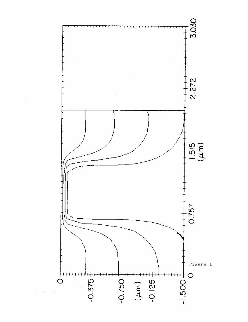
k conventional single exposure method used to open a . 5 u m line is shown in Figure 3a. The four electron-beam ppots have a FWHM of ,125 um and were thus spaced accordinglyi at 8 spotsium density. The dose was 45.6 uc / c m 2 and each spot

- 4 -

was weighted equally (given an equal share of the total dose). The developed contours correspond to development times of 40G to 600 seconds in 20 second intervals. A s can be seen, the contours about the . 5 um nominal linewidth are Dvercut and rounded with the linewidth increasing at a rate o f . 0029 um/sec.

In an effort to improve on the developed profiles o f Figure 3al the relative doses of the four beam spots were adjusted while keeping the total dose the same. In efffect, the two middle spots were given approximately four times) the

The developed cont ursl corresponding t o development times of 260 to 400 secon 1 s in dose o f the outer two spots.

20 second intervalsl are shown in Figure 3b. In this dase, the sidewalls are more vertical and the linewidth is adqanc- ing at a lower rate o f .a021 um/sec about the . 5 um nominal 1 inewidth.

In Figure 4, the reduced spot writing scheme of Greeneich C 9 1 is simulated. This method uses only two spots spaced at a distance equal to twice their FWHM value C.125 um). The total dose was again 45.6 uc/cm2. The developed contours correspond to development times of 280 to 480 seconds in 20 second intervals. The contours are slightly improved over the contours of Figure 3a in that the ,sidewalls are slightly more vertical and that the linewidth is advancing at ,0026 um/sec about the . 5 um point.

Several versions of the initial resist thinning approach were explored in attempting to obtain greater linewidth control and improved shape. The first method simulated was simply a normal four spot initial exposure, as in Figure 3 a l at half the dose (22.8 uc/cm2) and an identical secondary exposure at a depth in the resist o f . 5 wm as illustrated in Figure 5a. The contours correspond to development times of 700 to 900 seconds in 20 second imter- vals. The sidewalls are more vertical and the linewidth is advancing at .0021 um/sec-which is an improvement over both the conventional technique of Figure 3a and the two spot approach of Figure 4.

This resist thinning process can be further improved b y assigning different weights to each o f the exposure s(pots. The method which appears to give the most significant improvement is shown in Figure 5b. The initial exposure is still four spotsi howeverr the middle spots were given five times m o r e dose than the outer spots. The secondary exposure then utilized only two spots directly below the initial two middle spots at a depth of . 5 um. The secondary exposure was given three and one-half times more dose than' the initial outer spots. The total dose was still constr ined to be 45.6 uclcm2. The developed contours correspon to development times of 280 to 480 seconds in 20 second i I! ter- vals The contours show significant improvement over

- 5 -

results o f previous techniques. The sidewalls are verttical and the linewidth is developing out at a m u c h slower rate, ,0013 um/sec about the . S um nominal linewidth.

For comparison purposesl the use of two spots sitqilar to those used in the preceding secondary exposure were imu- lated using a conventional approach. Contours correspo d i n g to development times of 200 to 400 seconds in 20 s i cond intervals at a dose of 45.4 uc/cm2 are shown in Figur4 6.

ing at a rate of ,0018 um/sec about the nominal . 1 inewidth.

The sidewalls are slightly curved and the linewidth is

A plot of linewidth versus development time for the various exposures discussed is shown in Figure 7. As c$n be seenl the various strategies have slopes w h i c h diffed b y over a factor of 2. The optimized initial resist thiflning procedure gives about 28% better linewidth control (deained as the slope of the curve about the . 5 um nominal linewidth) over the two spot exposure of Figure 4, a 40% improv over the weighted conventional exposure technique of F 3 b l a 30% improvement over the technique of Greeneic Figure 4, and a 35% impravement over the conventional nique of Figure 3a.

Profile Description Parameters I

We now attempt to quantify the comparison of resist profiles b y introducing a set of profile description palrame- ters. The quantities x ( 0 ) , x(.4), and x(.8) are defined as the half-linewidths at the relative remaining resist thicknesses of (3, .41 and .8, respectively. The definition o f these parameters is illustrated in Figure C81. Notelthat the the . 8 level allows for reasonable top loss of resi8t.

From these three direct profile parameters, two independent quality parameters can be calculated.

T : or angle f 1 0 3 of the sidewalls is specified b y the

T = (X( .d)-X(0))/.8th

where t h is the resist thickness. This is equivalent to the inverse slope of the straight line connecting the resist openings at x ( . 8 ) and ~(0). The curvature of the side+alls is described b y the quantity, C:

C = ( x ( . 4 ) - . 5 ( ~ ( .8)+x(O)))/.8th

C is the horizontal distance from the resist openin at x ( . 4 ) to the straight line which defines T. These qu nti- ties a r e also shown in Figure 8. Normalization o f the i bove

- 6 -

X R o ~ d e r t o make comparisons with the optimum profiles for a particular process, a process performance

quantities is made to resist thickness and not lineiwidth .zince the quality of a resist edge profile is primarily1 due t o exposure beam quality, electron scattering, and dev loper effects and is only related to linewidth to second ord f r.

desired

where Aef f is the deviation from the optimum, Tn is the t i l t of ths desired profile and Cn is the curvature oif the desired profile Thus, a Aef f = 0 indicates a perfect imatch between an experimental or simulated profile and/ the optimum. A figure of merit to describe a given profille is thus defined as:

Q = . 8 t h / A e f f

Thus, This is normalized to include the Tesist thickness. the closer a profile corresponds to the desired resist^ pro- f i l e , the higher will be the Q value. It should be lnoted that the analysis allows almost any type of nominal prlofile shape to be used ( f o r example, undercut profiles when com- paring profiles for certain liftoff processes).

It is more difficult to define the bias or diff rence in half-linewidth between the actual and optimum pro ,iles. A useful definition must reflect the position of the p rtion o f the resist profile, X R , w h i c h is critical to the p ttern transfer process. More importantly, it must also implicitly define what is meant b y the nominal exposure half-line i idth, X E . Qne definition of X E which we find convenient,' and only slightly ambiguous, is the 50% exposure dose leqel of the n e a r e s t written spot or beam edge.

However, to emphasize the difference in bias foq the various writing strategies in this paper, X E is assu ed to be .2.5 um for all the patterns. Furthermore, the d 1 sired optimum profile is chosen to have zero tilt and curv T h e bias, B, which in general is defined to be the dis

-1 . I L , ~ L desired profile is vertical, X R I is chosen t o be The value of X ( . 8 j when the t i l t is zero. That is, B is the over or under developed distance from the nominal . 2 p urn half-linewidth at which the developed profile has zero tilt ! F i g u r $ e 81

tern. Finally, the relative merits of a particular

TG complement the quantitative description of profile shapef an expres5ion is needed which will reflect the sknsi- tivity o f t h e feature size to development time. The sbnsi- tivity can be defined as:

approach

where td is t h e development time. A figure of merit for development time effects is thus:

FM = 1 / S

These profile description parameters allow the dibcus- sion of resist profile quality f o r the various writing stra-

expected, the four-spot conventional approach of FiguRe 3a has both a low F.M. and Q-indicating poor shape quality and linewidth control. I t also has a very large bias o f more than 0.14 urn. The weighted four spot approach shows sligni- ficant improvement in linewidth sensitivity as well ps in shape and bias. The two spot appvoach of Greeneich hbs a similar profile quality but a lower development figuse of merit than the weighted four spot method. The four spot thinned approach of Figure 5a shows that the thinning kech- nique can improve curvature and quality. However, the developer figure of merit is degraded slightly. The optimized thinned approach of Figure 5b shows a very significant improvement in both quality and developer figure of merit while maintaining a small bias. The two spot conventliondl exposure of Figure 6 also shows similar improvements bult has a noticeably larger curvature.

tegies to be restated more quantitatively (Table 1 ) . A s

- 8 -

development parameters.

Investisation of the Resist Model

Now let us turn to the problem of improving the apree- ment between simulation and experimental resist prolfiles presented earlier C 1 1 . The initial approach was to fukther explore fine tuning the development model parameters; but, little impart could be made. For example, making the beam size smaller in an attempt to eliminate the rounded bbttom o f the simulated profile resulted in the top corners bkcom- ing t o o sharp with little change in the bottom. The lshape o f the etch rate versus dose curve was also adjustekl b y changing DO, a and R l i but, again there was no significant improvement. Thus, we conclude that to achieve b agreement with experiment, the basic resist develo model must be generalized.

As a second approach, the development model was generalized to allow the development of the resist to toccur moT'e rapidly approximately along the direction of the primary electron trajectories. This anisotropic effeclt was implemented approximately b y a fractional reduction in the lateral motion of the nodes in the string algorithm ias is illustrated in Figure 9. Figure 10 is a comparisob of experimental and simulated profiles from E 1 1 and simullated profiles with a 70% reduction in lateral development. The adapted profiles correspond to development times of E O to 180 seconds in 20 second intervals. The experimental contours from E 1 1 correspond to a 180 second development1 time while the simulated profiles from E l l correspond to dedelop- ment times of 20 to 200 seconds in 20 second intervals. All other parameters are the same as in E l l .

For the case of isolated lines in Figure 10, the p r o - files with this simple reduction in lateral developmend rate more closely track the experimental contours. However, for arrays of lines in Figure 10, the correction was n/ot as necessary. A possible explanation is that development tends to occur more rapidly along the trajectories of the h i g h energy electrons. The physical mechanism causing suclh an effect might be related to the generation of volatild pro- ducts and micropores during exposure C 1 1 1 . This prefleren- tial development along trajectories is consistent with there being more of a need to correct the simulated profiles for isolated lines as compared to arrayed lines. F o r dingle lines, the electron trajectories would be fairly vedtical with spreading increasing with depth in the resist. For arrayed linest however, proximity effects contribute a significant mix of non vertical backscattered electrons which

Although the basic physical mechanism is not clear, t h simple addition of a preferential development factor appe efdects* rs to

would tend to average out the preferential

be a simple procedure f o r significantly improving the

- 9 -

agreement o f simulated profiles with experiment.

Conclusion

One of the advantages o f simulation is its flexibility to explore potential processing approaches. Various assump- tions have been used to explore writing strategies anid an improved resist model for electron-beam lithography. An initial resist thinning and secondary exposure particullarly applicable to contact opening has been suggested. P r file description parameters have been introduced to evaluate profile shape and linewidth sensitivity more quantitati ely. These parameters show that b y weighting the middle spots m o r e heavilq or reducing the number o f spots/line imp ~ oves the profile shape as well as the sensitivity to develo ment time.

The initial dependent bias into the exposure pattern. resist thinning approach was also shown to result in fu ther improvements in both profile quality and linewidth siensi- tivity. Several possible exposure and resist develolpment effects were explored to improve the detailed fit of simulation to experimental line-edge profiles. Introducing a1 pre- ferred anisotropic etching approximately in the directilon of the primary electron trajectories was found to give a sligni- ficant improvement in the comparison, especially for isolated lines.

This corresponds to designing a resist thickness i" b

Ac knowledciment

The authors would like to thank C . H . Ting, D.F. Wyser, S. N. Nandgaonkar, and Y . C. Lin for valuable discussions' during the course of this work.

Research sponsored b y the National Science Foundation Grant ENG77-14660 and IBM Fellowship.

Parts of this paper were originally presented at the gpring 1980 meeting of The Electrochemical Society, Inc. h d l d in St. Louis, Missouri.

- lQ, -

Re- ferences

c 1 1

C21

E31

C41

C53

C61

C71

C 8 1

C 9 1

E 101

[ i l l

D.F. Kyser and K . Murata, Proc. 4th Int. Conf. ctn Elec- tron and Ion Beam Sci. Tech. (Electrochemical Society, 1974), R. Baltish, ed. , p p 205-223.

I. Adesida, "Electron Energy Dissipation in Layered Media", P h . D dissertation, Dept. of EECS, U . C . Berke- ley, 1979.

H . E . Jewett, P. I. Hagouel, A . R . Neureuther, and T. Van Duzer, Polymer Eng. Sci. , vol. 17, no. 6 , p p . 381-384, 1977.

W . G. Oldham, S. N. Nandgaonkar, A. R . Neureuther, and M.M. O'Toole, IEEE Trans. Electron Devices, vol. ED- 26, no. 4, p p . 717-722, 1979.

W . G . Oldham, 4. R. Neureuther, C. Sung, J . L. Reynolds, and S. N. Nandgaonkar, IEEE Trans. Electron Devices, v o l . ED-27, no. 8, p p . 1455-145'7, 1980.

M. G. Rosenfield and A. R. Neureuther, Proc. 9th Ink. Conf. on Electron and Ion Beam Sci. Tech. (Electrochem- ical Society, 1480), R. Bakish, ed., p p . 382-395.

J . S . Greeneich, J. V a c . Sci. Technol., vol. 16, no. 6, p p . 1749-1753, Nov. /Dec. 1979.

M. Hatrakis, J. Vac. Sci. Technol., vol. 12, no. 6, p p . 1276-1279, NOV. /Dee. 1975.

A.C. Uuano, Polymer. Eng. Sci. I vol 18, no. 41 p p . 306- 313, 1978.

- 1 1 -

Fiqure Captions

1.

2.

3.

4.

5 .

#I.

7.

8.

9.

10.

Local initial resist thinning strategy

Local initial resist thinning simulation approach

Simulation o f conventional exposure techniques. a ) Equally weighted spots b ) Weighted spots -- inner spots have 4 times the dose o f the outer spots.

Simulation o f reduced spot technique -- two spots equa 1 1 t.~ weighted.

Simulation o f local initial resist thinning technilques. b ) a ) Identical initial and secondary

Weighted initial exposure -- inner spots have 5 times the dose o f outer spots, secondary exposure spots have 3.5 times the dose of the outer spots.

e O S ur T

Simulation o f a two spot conventional exposure similar to the secondary exposure o f Figure 5 b .

Linewidth versus development time for the various exposure techniques.

Table 1 -- Profile description parameters for the various exposure techniques.

Illustration of some o f the profile description pqrame- ters in Table 1.

Reduction o f lateral motion o f string nodes in the development model. ( 1 - a 13 100% is the reduction.

Comparison o f earlier simulated (left) and experidental (middle) resist profiles C l l with simulated prdfiles corresponding to a 70% reduction in lateral tring

Simulated contours correspond to 20 motion (right). second intervals. Experimental development time i s 180 seconds.

1

- . t \ I?

I t \ 1 \ 1 < t f t - \ I \

\ \ / 1 \ yy' y-*{

Figure 1

r

Res is t

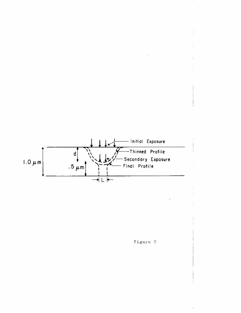
LOprn

Init ial Exposure

\ \ \ \ / Y-Thinned Prof i le

k4tL Final P r o f i l e

r -

d \:\ll$$’- Secondary Exposure

I I . 5 p m (f

Figure 2

I

I

I

0 0 m N

0 I

0 0 m 0

I 0

I

Figure 3a

0 0 0

I

0 0 Ln cv 0

I

0 0 Ln

0 I

0 L n b

0 I

0 0 0 . -

I

Figure 3b

0

0 -

0 m 0

0 0 0 0 0

0 0 b 0

0 0 cu 0 0 0 -

I 0 I I I

0

W)

Figure 4

0 0 ln N

0 I

0 0 ln 0 I

0 Lo w 0 I

0 0 0 I

Figure 5a

0

- 0.250

- E -0.500 =t -

-0.750

-1.000 0 0.50 I .o

( p m )

Figure 5b

0 ln 0

A cv

0 0 0

0

Lo cu I

0 0 Ln

0 I

0 u3 b 0

I

0 0 0 - I

Figure 6

.30

.20' 200 300 400 500 600 700 800 900

DEVELOPMENT TIME ( s e d

u) M

00 cn m 0 cn In d- (0 n J 0 0 0 0 0 0

m W

m cu 0

In In

- W

- u)

r- e

a0 In cv

- 00 cu

Tt a0 *

In * m

0 Lo m

In cn * 0 Tt rc)

CD cn - <v CV cu 0 0

0 0

0 0

- cu 0 0 0 . 0

d- F 0

0 00 0

0 cu 0

- ' 0 j v-

* 00 (0 0

m cu 0

0 c 0

c a > C 0 0

0 a v)

-- c

I c

0 rc)

E 3 9,

L L .-

T3 Q,

c 0 a

I

c

.- 3 0 Q v)

c

* t! 3 9, LL .-

-0 Q, C C .c t I c

.-

0 v) n

d * (v *

'0 Q, c c c .- c

I

3 E E n 0

.- t

n In

t! 3 0 LL .-

0 C 0

t Q) > c

.- t

' E I t 0 0 v)

nJ I

I t I I

1

-------- I- - - -\-- L r-

I

c t

00 c t * c

t

0

Figure 8

I

St r

n-l

i"g \velopef

R e s i s t &

Figure 9

Appendix I 1 1 -- Common Block Description

/ANRATE/

Anisotropic rate is common to subroutines ECYCLE, EBMSG(numb), TRLlOl, and TRL112.

FRAC -- the fraction of the normal horizontal motion deqired in the development algorithm (cf. Trial 112, arg3).

/CELL/

Cell size is common to the Controller and subroutines MLTLIN(numb), EBMSG(numb ) , EPLOT, SQWGT, SPWGT, and TRLIO1.

CELLX -- the M/C cell size in the horizontal x direction in microns.

GEL-LZ -- the M / C cell sire in the vertical z directioq in microns.

/CNVLVl/

Convolution block 1 is common to the Controller and su tines MLTSPT, EGAUSS, WEIGHT, PRARRY, MLTLIN(numb1, EA EBMSGtnumb), SQWGT, SPWGT, TRL101, TRLlll, and TRLl13.

NCLMET -- the number o f locations used in the grray ETEM2 999 ) .

DEVUNI -- temporary storage for the standard deviation b f an exposure spot.

DEVTEM -- temporary storage for the standard deviation o f an exposure spot.

DOSE -- the dose in uC/cm**2 given to the overall expbsure pattern C c f . Trial 1 1 1 a r g 2 and T r i a l 113 arg2).

/CNVLV2/

Convolution block 2 is common to the Controller and subroutines EGAUSS, WEIGHT, PRARRY(numb ) I EARRAY, EBMSG(nbmb 1 1 SQWGT, SPWGT, and TRL101.

EMAT(#Of500) -- a t w o dimensional array containing the1 M/C data used in the convolution o f the e-beam exposure pat ern.

- 2 -

NUMSPT -- a counter used to keep track of the numbev of spots making u p a line.

WGHTQ --- temporary storage for the ‘weight‘ given a spot

NCEMAT -- the number of columns used in the array EMAT (801 500 ) .

/COPY WD /

SAMPLE copy window C81 is common to the Controller and subroutines EBDEV, EPLCIT, TRLlOl, and TRLllO.

CPWIND -- the resist window of interest size in microns €cf. Trial 110 arg23.

CPEDGE -- 1/2 CPWIND, used in SAMPLE plotting routines. ~

CPWORG -- not used b y the e-beam machine. I

I

/DEVFLG/

SAMPLE develop flag C81 is common to subroutines EBDEV and TRLlO1.

IDEVFL(5) -- a one dimensional array containing the flags for the development machine. 1 means ‘yes‘ and 0 (neans ‘no’. IDEVFL(1) -- print the number o f string pointsl etc. and subroutine CHKR point totals? IDEVFL(2) -- print out points for each profile? IDEVFL(3) -- set equal to more points for more time-consuming but more accurate runs.? (cf. Trial 2 argl arg2 arg33 IDEVFL(4) and IDEVFL(5) are not used b y the e-beam machine.

/DEVTIM/

SAMPLE development times C81 is common to subroutines EQDEV, EBMSG(numb ) , and TRL101.

MXNDEV -- the maximum number of development contours that can be Tequested b y the user -- currentlq 20 €cf. SAMPLE Key-word ‘devtime‘ arg33.

DEVSRT -- the development time in seconds of the first development contour € c f . SAMPLE key-word ‘devtime’ argll3.

the development time in seconds o f the inal development contour ( c f . SAMPLE key-word ‘devtime’ arg 3 DEVEND --

DEVINC -- t h e time in seconds between the intermekliate 1 eve 1 o p men t c onto ur s .

F I

- 3 -

/DFALTl/

CteFavlt b l o c k 1. i:s common to the Controller and subroutines TRL-101 and TRL110.

ISYM -- a flag in which '1' indicates a sqmmetrical dev$lop- ment ( c f . Trial 110 ar331

SHFDIS!Z?O) --- a one dimensional array containing t h e positions o f t h e cpots in an exposure line Xcf. Trial 106 arg3 o r Trial 107 arg3, argb, etc. 3.

DISLIN(20) -- a one dimensional array containing the positions o f the lines in an exposure pattern €cf. Triak 108 a r g 3 or T r i a l 109 arg3 , arg5, arg7, etc. 3.

SPTWGT(20) --- a one dimensional array containing the weight f o r each spot in an exposure line Xcf. Trial 106 arg5, ergb, etc. o r Trial 107 argSf arg8, etc.3.

IJGTLIN(20) -- a one dimensional array containing the weight f o r each exposure line Xcf. Trial 108 arg4, arg5, ett. or Trial 109 arg4, arg6, etc. 3.

STDDEV(20lt -- a one dimensional array containing the stan- d a r d deviation o f each spot in an exposure line (cf. Trial 106 a r g 4 o r Trial 107 arg4, arg7, etc.3.

ITCOU -- the number o f spots in an exposure line (cf. Trial 106 arg2 o r Trial 107 arg21.

/DVELP 1 /

SAMPLE development block i C 8 1 is common to subroukines EBDEV, ECYCLE, TRL-101, TRLll2, and function EBRATE(ct).

XZ(1000) -- complex array containing the x and L posiltions o f the 1000 possible development string points.

XMAX -- the real (not including boundary) maximum value/ o f x in microns.

ZMAX -- the real maximum value of z in microns. I I

NPTS -- the current number of development string points Ccf. Trial 112 a rg2) .

- 4 -

C X Z L -- the normalized left endpoint direction o f development.

CXZR -- the normalized right endpoint direction NADCHK -- the number o f advances (calls on subroutine ECY- C L E ) between checks (calls on SAMPLE subroutine CHKR CSfr3.

NCH.C)UT -- the number of checks between outputsi the nvmber o f advances between outputs is NADCHK*NCKOUT.

/ D V E L P 2 /

SAMPLE development block 2 E 8 1 is common to subroutines E B C Y C L E and EBDEV.

TADV -- the current time between advances ( f o r subroutine ECYCL.E) .

TCHK -- the current time between checks. TTQT -- contains the total current development time during the execution of the SAMPLE-E-BEAM development machine.

I F L A G -- flag set in E C Y C L E that tells EBDEV that some string segments are too long or too short. SAMPLE su routine CHKR is then called from EBDEV.

SMAXX -- the maximum x string segment length allowed b y / C H K R (and E C Y C L E i .

P

S M I N X -- the minimum x string segment length allowed b y CHKR.

SMAXZ -- the maximum z string segment length allowed b y C H K R .

/ D V E L P 3 /

SAMPLE development block 3 C81 is common subroutines E C Y C L E and E B D E V .

N Z F L G -- a flag used between subroutines E B D E V and E C Y C C E in order to signal when the string has broken through the resist. T h e number of checks between output5 is then reduced.

NADFLG -- the output number of the string that broke thkough the resist.

/ D V E L P 4 /

- 5 -

SAMPLE development block 4 E 8 3 is common to subroutine EBDEV.

BREAK -- the estimated time until resist breakthrough

MAXPTS -- when the number of string points exceeds MAXPTS, SAMPLE subroutine DELOOP is called.

NADSAV -- contains the NADCHK before resist breakthrough. NCKSUl -- contains NCKOUT before resist breakthrough fot. the first development output.

NCKSV;! -- contains NCKOUT before resist breakthrough f o t the intermediate outputs. ~

1 I

NOWT -- the number of development outputs requested Ccf. SAMPLE Key-word 'devtime' arg33.

/ ENGPLT /

Energq plotting is common to subroutines EBMSG(numb), EPLOT, TRL101, TRLllJ.

IDEP -- the first row (not including boundary) of the ELIN(82,1002) array to be printed Ccf. Trial 115 arg3).

ISKIP -- the skip number of rows of ELIN(82,1002) tb be printed ( i . e . rows IDEP, IDEP+ISKIP, IDEP+ISKIP+ISKIP, etc. are printed out) € c 9 . Trial 115 arg43.

IR1 -- a flag in which a 1 indicates that in the outpuk of the energy plotting option €cf. Trial 1153, the value oiF the maximum absorbed energy density in the desired row15 of ELIN(82,lOOZ) is printed in the output file. If IRI it5 any other positive integer number, that number is the malximum absorbed energy density printed. This maximum energy density 1 s printed before the actual energy density values and is only used to give a range o f the energy density f o r plotting purposes (rf. Trial 115 arg23.

ENGMAX -- a maximum value of absorbed energy density prlinted for plotting purposes.

/HORIMG/

SAMPLE horizontal image t83 is common to the Controlller, subroutine EBDEV, and function EBRATE.

DELTX -- the size of the M/C cell in the horizontal x diirec- tion in microns.

- 4 -

NMHPTS -- the number of columns (including boundary) used in the array ELIN(82,1002) to describe the absorbed energy density in the window of interest.

MNHPTS --- not used b y the e-beam machine.

HORINT(5O) -- not used b y the e-beam machine.

SAMPLE input-output block 1 is common to the Controller and subroutines PRARRY(numb), MLTLIN(numb1, EBDEV, EBMSG(numb), SQWGT, SPWGT, and all TRLxxx subroutines.

All o f the variables in this common block are assigned numbers appropriate to the computer system in use an# are

‘READ(IBULK,#) variable’ are used to output and input information and data.

used in input-output. For example, ‘WRITE( IPRINTI # ) ‘,

/LINEi/

Line block 1 is common to the Controller and subroutines PRARRY(numb), MLTLIN(numb), EARRAY, EBDEV, EBMSG(nbmb), BQUNDRt EPL-OT, TRL101, TRLl08, TRLl13, and funktion EDRATE( c z ) .

ELIN(82, 1002) -- a two dimensional array containing the absorbed energy density in the resist window o f intereslt due to a specified electron-beam exposure.

LCOU -- the number of lines in the exposure pattern ( c f . Trial 108 arg2 or Trial 109 arg23.

LINCC3U -- also the number of lines in the exposure paktern (redundancy due to changes in the original e-beam propram; the variable was left in due to the author’s laziness).’

ELNWGT(l999) -- a one dimensional array containing the botal exposure pattern needed to determine the absorbed ebergy density in the window of interest.

/LINE2/

Line b l o c k 2 is common to the Controller and subrou ines

EBMSG(numb ) , EPLOT’, TRL101, and TRL113.

NCELIN -- the maximum number o f columns which can be uskd in the array ELIN(82, 1002).

PRARRY (numb MLTLIN(numb), EARRAY (numb ) BO L NDR,

- 7 -

NWMCOL -- the number o f array locations in EMLT(1499) used.

MAXCOL -- the number of columns (not including boundary) of ELIN(82,1002) used (Note that MAXCOL is used f o r a diffkrent p u ~ p o s e in the Controller -- to determine the locatioh of the left window of interest edge f o r a symmetric development).

NCEMLT -- the maximum number of array locations in EMLT(1499) which can be used.

NCLELU -- the number o f columns (including boundary) used in the array ELIN(82, 1002).

NRELIN .-- the number o f rows in the array ELIN(82,k002) used.

/MCARLO/

Monte Carlo information is common to the Controller and subroutine EBMSG(numb).

THICK -- the thickness o f the resist in microns.

EVENG -- the energy o f the e-beam in KeV.

/PARSEM/

SAMPLE parsem is common to subroutine EXTRA6 and all TflLxxx subroutines except TRL101.

STNMLS(i00) -- a one dimensional array which contains the values o f each o f the arguments in a Trial statemeht or Key-word,

NMINST -- the number of arguments set b y the user in a Trial statement or Key-word.

ISTMTY -- not used in the e-beam program.

ISTKND -- not used in the e-beam program.

NMPNTR -- not used in the e-beam program.

/PRFLG/

Printing flags is common to the Controller and subrou ines PRARRY(numb) WEIGHT, SQWGT, TRLlOl, and TRL102.

ILJFLG(5) -- a one dimensional array containing the Iflags !L=yesf which influence the output of information and

1

- 8 -

messages b y the program (cf. Trial 102 with abg2-6 corresponding to IWFLG(1-5)).

/RATDAT/

Rate equation data is common to subroutines EBMSG(numb), TRLl01, TRL104, and function EBRATE(cz1.

(Rl*CM) -- the background etch-rate in A/sec €cf. Trial 104 arg2 arg31.

DO -- a reference or knee energy (cf. Trial 104 arg4)

ALPH -- the asymptotic slope of the etch-rate vErsus absorbed energy density curve for the resist at h i g h dose € c f . Trial 104 arg5).

/SDIST/

Shift distance is common to the Controller and subroukines MLTLIN(numb)f EBMSG(numb), and TRLl10.

SHIFT -- the distance in microns of the first spot or rectangular beam from the left window edge €cf. Triak 110 arg41.

/SIMPAR/

SAMPLE simulation parameters C81 is common to the Con- troller, subroutine EBDEV, and function EBRATE(cz1.

NPRLYH -- the number of layers the resist is to be divided into ( i . e. the number of rows used in ELIN(82, 10021) not including boundary).

NPRPTS .-- n o t used in the e-beam program.

NENDIV --- not used in the e-beam program.

DELTM -- not used in the e-beam program.

DELTZ -- the size of the M/C cell in the vertical z dlirec- tion in microns.

/SPOTl/

Spot block 1 is common to the Controller and subroutines MLTSPT, EGAUSS, WEIGHT, PRARRY (numb 1 , MLTLIN(numb ) , EAkRAY, SPWGT, and SQWGT.

ETEM2(999) -- a one dimensional array containing the

- 9 -

exposure pattern profile o f a single Gaussian spot or rectangular shaped electron-beam.

EMLT(1499) -- a one dimensional array containing the exposure pattern profile f o r a single line.

/SPOT2/

S p o t block 2 is common to the Controller and subroukines MLTSPT, EGAUSS, WEIGHT, PRARRY(numb MLTLIN(numb ) I EARRAY, EBMSG(numb) TRLlOl, TRLllS, SPWGT, and SQWGT.

ISHIFT -- an integer counter used to keep track o f the distance in array units between spots in a line. I

WGHTl -- temporary storage f o r the 'weight' given a s p o b .

NRHCET .-- the number o f array locations used in the right hand side (not including center) o f ETEM2(999).

I

NREMAT -- the number o f rows used in the M/C array EMAT (801 500 I .

/SQBEAM/

Square beam is common to the Controller and subroultineo SQWGT, TRLiOl, and TRLlOS.

ISQ -- a flag in which 1 indicates a rectangular beam 'exposure line.

FWHM -- the full-width half maximum o f the rectangular beam in microns C c f . Trial 105 arg21.

EDGE -- the edge-width o f the rectangular beam in miicrons ( c f . Trial 105 arg3).

AoDendix -- Program Code

c SUBROUTINE EXTRIA calls the e-beam trial statements C

subroutine extria(if1ag) common /parsem/ istmty, istknd, stnmls(100), nminst, nmpntr

itest=int(stnmls(l)) if (itest .ne. 101) go to 102

C

c trial 101 initializes default parameters f o r e-beam si ulation call trllOl t return

C

102 continue

c trial 102 initializes printing flags for a r r a y ~ ~ m e s s a g e s if (itest .ne. 102) g o to 104

call tr1102 return

C

clO3 continue C if (itest .ne. 103) go to 104 c trial 103 tells program which M/C file to use C call trll03 C return

104 continue

c trial 104 initializes rate eqn. parameters

C

if (itest .ne. 104) go to 105

call trl104 r et 11 r n

C

105 continue

c trial 105 is f o r square shaped beams if (itest .ne. 105) go to 106

call tr1105(11 return

c 106 continue

c trial 106 is for gaussian shaped beams--periodic if (itest .ne. 106) go to 107

call trllOS(2) return

j i 107 continue

c trial 107 is for gaussian shaped beams-non-periodic I

C

j if (itest .ne. 107) go to 108

call trll05(3) return

- 2 -

C 108 continue

c trial 108 is f o r periodic line arrays if (itest .ne. 108) go to 109

call tr1108(1) return

c 109 continue

c trial 109 is for non-periodic line arrays if (itest .ne. 109) go to 110

call tr1108(2) return

c 110 continue

c trial 110 sets type o f develop, window size, and position in window c if non-sym. develop

if (itest .ne. 110) go to 1 1 1

call trlllO return

C

1 1 1 continue

c trial 1 1 1 sets the exposure dose and r u n s the convolution if (itest .ne. i l l ) go to 112

call trllll return

C 112 continue

c trial 112 sets dev. times, npts, anrate fraction if (itest .ne. 112) go to 113

call tr1112 return

C 113 continue

c trial 113 sets new dose f o r elin array if (itest .ne. 113) go to 114

call tr1113 return

C 1 1 4 continue

c trial 114 runs the develop programs if (itest .ne. 114) go to 115

call tr1114 return

C 115 continue

c trial 115 is the energy profile option if (itest .ne. 115) go to 116

call trlllS return

C 1 1 6 continue

if lag=O return end

- 3 -

f C C

C C C

C

C

C

C

SUBROUTINE TRLlQl initializes default parameters

subroutine trllOl common /spot2/ ishift, wghtl, nrhcet, nremat common /line2/ ncelin, numcol, maxcol, ncemlt, nclelu, nrelin common /cnvlvl/ nclmet, devuni, devtem, dose common /cnvlv2/ emat (80, S O O ) , numspt, wghtO, ncemat common Iratdatl rl, cm, d 0 , alph common /distnc/ shfdis(20), dislin(20), sptwgt(2O),wg$lin(20),

common /prflg/ iwflg(5) common /iol/ itermi, i b u l k , iprout, iresvl, iin, iprint, punch common /linel/ elin (82 , 1002), lcou, lincou, elnwgt ( 1 99)

common /devtim/ mxndev,devsrt, devend,devinc common /dvelpl/ c x z l , cxzr, xz(lOOO), xmax, zmax,npts,nLdchk,nckout common /copywd/ cpwind,cpedge,cpworg common /anrate/ frac common /sqbeam/ isq, fwhm, edge common /dfaltl/ isym common /engplt/ idep, iskip, irl, engmax integer dO complex X Z , c x z l r cxzr iprint=&

* stddev(20), itcou

common /devflg/ idevfl(5) t

this is the default initialization routine set flags to print out only info.

iwflg(l)=O iwflg(2)=0 iwflg(3)=0 iwflg(4)=0 iwflg(5i)=l

rate curve data ri=l. 0 cm=l. 0 dO=199 alph=2. 0

dose dose=80. 0

square beam option isq=l fwhm=l. 0 edge=. 25

periodic line option dislin(l)=O. 0 dislin(2)=2. 0 dislin(3)=4. 0 wgtlin(l)=l. 0 wgtlin(2)=1. 0 wgtlin(3)=1. 0 lincou=3

idevfl(l)=O develop flags

- 4 -

idevfl(2)el idevfl(3)=0 idevfll4)=O idevfl(5)=0

devsrt=40. 0 devend=l60. 0 devinc=40.0 npts=60

isym=l cpwind=2. 0 frac=l. 0

idep=l iskip=7 irl=l call ebmsg(23) write (iprint, 10)

return end

c develop times

c symmetric develop option

c energy plotting option

10 format(lxt33hE-beam default values initialized/)

- 5 -

SUBROUTINE TRL102 common /prflg/ iwflg(5) common /parsem/ istmtyJistkndJstnmls(lOO)JnminstJnm#ntr common /iol/ iterrnil ibulk, iprout, iresvlJ iinJ iprint, tpunch

C

c this trial sets the e-beam printing flags for arraysJ i$fo. C

if (nminst . ge. 2 .and. nminst . le. 6 ) go to 20 write(iprint, 10)

10 format(lxJ39hERROR-Tria1 102 requires a minimum of pJ * 39h and a maximum of 6 arguments to changeJ/ * 1xf32hthe default ebeam printing flags/) return

C

20 continue

5 iwflgC5)=int(stnmls(6)) 4 iwflg(4)=int(stnmls(5)) 3 iwflg(3)=int(stnmls(4)) 2 iwflg(2)=int(stnmls(3)) 1 iwflg(l)=int(stnmls(2))

go to ( 1 , lJ2J3J 4, 5 ) nminst

return end

SUBROUTINE TRL104 common /ratdat/ r l J cmJ do, alph common /parsem/ istmty~istknd,stnmls(lOO)JnminstJnm~ntr common /io11 itermi, ibulk, iprout, iresvlJ iinJ iprintJ lipunch integer d 0

C

C c this trial sets rate eqn. constants C

if (nminst . ge. 2 .and. nminst . le. 5 ) go tu 20 write(iprintJ 10)

10 format(1xJ39hERR0R-Tria1 104 requires a minimum o f 2, * 39h and a maximum of 5 arguments to changeJ/ * 1xJ36hthe default rate equation parameters/) return

C

20 continue

4 alph=stnmls(5) 3 dO-int(stnmls(4)) 2 cm=stnmls(3) 1 rl=stnmls(2)

return end

SUBROUTINE TRLlOS(numb) common /parsem/ istmtyJ istknd, stnmls(lOO)J nminst, n pntr common /sqbeam/ isqf fwhmJ edge c ommon / d is tnc / sh f d is (20), d is 1 in (20) sp twg t (20) wg/t 1 in (20)

common /iol/ iterrnil ibulkJ ipruut, iresvlf lint iprint, ipunch

g o to ( 1 J 1#2,314) nminst

C

nj

* stddev(20lJ itcou

- 4 -

C

c this subroutine sets the incident exposure line shape (trials 105, c 206, 107) C

c initialize arrays to zero do 95 i = l t 2 0

shfdis(i)=0. 0 sptwgt(i)=O. 0 stddev( i )=O. 0

95 continue go to ( 1 1 2 , 3 ) numb

C

c sq beam option 1 if (nminst . ge. 2 .and. nminst . le. 3) go to 20

10 format(1x139hERROR-Tria1 105 requires a minimum of pt * 39h and a maximum of 3 arguments to changet/' * lx134hthe default rectangular beam shape/)

write(iprint, 10) 1

return C 20 continue

5 if (stnmls(3) . le. 0.0) write(iprint, 19) 19 format(1x148hERROR-Tria1 105-an edge width less thafi or equalt /

go to (4,4,S) nminst

* 44h to 0.0 is not allowed for rectangular beem shape/) if (stnmls(3) . le. 0.0) return edge=stnmls(3)

4 fwhm=stnmls(2) isq=1 return

c periodic Gaussian option 2 if (nminst .ge. 6) go to 23

21 format(1x139hERROR-Trial 106 requires a minimum of Ist * 37h arguments(i.4. at least 2 spots) for,/ * 1xt38hthe periodic gaussian beamshape option//)

wr i te ( ipr int, 21 )

return

if (itcou . le. 20) go to 25 write( iprint, 24)

call ebmsg(7) return

write(iprintt 1 1 )

23 itcou=int(stnmls(2))

24 format(lx140hERROR-Trial 106-periodic gaussian optiicrn/)

25 if ((nminst-4) .eq. itcou) go to 30

1 1 format(1xt39hERROR-Tria1 106 requires specifying thkt * 37h same number of weights and spots f o r t / * 1x138hthe periodic gaussian beamshape optionr) return

write(iprint, 24) write ( iprint, 26)

return

30 if (stnmls(3) .ge. 0.0) go to 33

24 format(lx,3lhnegative spot shift not allowed/)

- 7 -

33 isq=0 call ebmsg(8) sper=stnmls(3) sigma=stnmls(4)

C c make shfdislstddev,weight arrays

stddev(l)=sigma sptwgt(l)=stnmls(5) do 99 n=2, itcou

stddev(n)=sigma shfdis(n)=shfdis(n-l)+sper sptwgt(n)=stnmls(n+4)

99 continue return

C c non-periodic Gaussian option 3 if (nminst .ge. 5 ) go to 34

32 format(lx,39hERROR-Trial 107 requires a minimum of 5, write(iprintl 32)

* 3 1 h arguments for the non-periodicl/ * 1x,25hgaussian beamshape option/) return

if (itcou . le. 20) go to 35 write(iprint131)

call ebmsg(7) return

if (itemp .eq. nminst) go to 40 write(iprint, 12) itemp, itcou

34 itcou=int(stnmls(2))

31 format(lx144hERROR-Tria1 107-non-periodic gaussian aption/)

35 itemp=(itcou*3)+2

12 format(lx,25hERROR-Trial 107 requires l i 2 1 1 0 h argumentsl * lbh to specify the i2, lbh spots requested] / * lx14Shin the non-periodic gaussian beamshape option/) return

do 190 n=3,itempt3 40 itemp=itcou*3

if (stnmls(n) .ge. 0.0) go to 190 write ( iprint, 31 ) write(iprint126) return

190 continue i = 3 isq=O do 199 n=llitcou

shfdis(n)=stnmls(i) stddev(n)=stnmls(i+l) sptwgt(n)=stnmls(i+2) j.=i+3

199 continue if (shfdis(1) .eq. 0.0) return write(iprintl 50)

50 fbrmat(lxl46hWARNING-Tria1 107-non-periodic gaussiai option, / * lx134hfirst spot does not start at x = 0 . 0 / )

- 8 -

return end

SUBROUTINE TRL108(numb) common /parsem/ istmty, istknd, stnmls(100), nminst, nmpntr common /distnc/ shfdis(20), dislin(20)) sptwgt(20)1wgtlin(20)1

common /linel/ elin (8281002),1cou,lincou,elnwgt (1999) common /iol/ itermi, ibulk, iprout, iresvl, iin, iprint, Spunch

C

3 stddev(20), itcou

C c this subroutine s e t s the positions of t h e exposure line$ (trials c 108 and 109) C

go to (1,2) numb

c periodic line array option 1 if (nminst .ge. 5 ) go to 5

4 format(1xt39hERROR-Trial 108 requires a minimum of $ 8

C

write(iprintr 4)

* 33h arguments(i.e. at least 2 lines),/ * 1xt28hfor the periodic line option/) return

5 l i n c o u = i n t ~ s t n m l s ( 2 ~ ) if (lincou .ne. 0) go to 20 write(iprint, 10)

call ebmsg(l1) lincou=3 return

write(iprint, 10) call ebmsg(12) lincou=3 return

write(iprint, 13)

10 forrnat(lx,42hERROR-Trial 108-periodic line array option/)

20 if (lincou . le. 20) go to 30

30 if ((nminst-3) .eq. lincou) go to 40

13 format(lx,39hERROR-Trial 108 requires specifying the, 3 37h same number of weights and lines f o r l / 9 1x,24hthe periodic line option/) 1 incou=3 return

C 40 if (stnmls(3) . g e . 0.0) go to 41

write(iprint, 10) write(iprint, 12)

lincou=3 return

41 call ebmsg(13) do 95 i=1,20

12 format(1xt31hnegative line shift not allowed/)

dislin(i)=O. 0 wgtlin(i)=O. 0

5 h f per=s tnmls (3 1 95 continue

- 9 -

C c put periodic line shifts in dislin(i), weights into wgtlin(i1

do 99 n=2, lincou 'isIin(n)=dislin(n-l)+shfper wg t 1 in tn-1 )=s tnmls (n+2!

99 continue IIMJ t 1 in I inc ou ) =s tnml s ( 1 inc ou+3) r e t u r n

C

I: non-periodic line option 2 if (nminst . g e . 4) go to 45

43 format(lxt39hERRQR-Trial 109 requires a minimum o f 4 , write(iprint, 433

* 3 1 h arguments for the non-periodic,/ * l x l llhline option/) return

4s lincou=int~stnmlsl2)) if tlincou .ne. 0) go to 44 write(iprint, 42)

call ebmsgcll) lincou=3 return

write(iprint, 42) call ebmsg{l2!) lincou=3 return

if (itemp .eq. nminst) go to 50 write(iprint1 14)itemp, lincou

42 format(ix,46hERROR-Trial 109-non-periodic line arraq option/)

44 if (lincou . le. 20) go to 48

48 itemp=(lincou*2)+2

14 format(lx,2ShERROR-Trial 109 requires ,i2,10h argumeints, * 1 6 h to specify the I i2, 1 6 h lines requested, / * lx131hin the non-periodic line option/) lincou=3 return

c 50 itemp=3 + (lincou-1)*2

do 190 nz3, i t e m p r 2 if (stnrnlstn) . g e . 0.0) go to 190 write(iprint, 42) write(iprint, 12) lincou=3 return

do 96 i=1,20 190 continue

dislin(i)=0. 0 wgtlin(i)=O. 0

96 continue i =3 do 199 n=l, lincou

dislin(n)=stnmls(i) wgtlintn)=stnmls(i+l) i=i+2

- 10 -

199 continue if (dislin(1) ,eq. 0.0) return write(iprintr 15)

call ebmsg(l4) return end

SUBROUTINE TRLilO common /parsem/ i s t m t y r i s t k n d r s t n m ~ s ( i O O ~ r n m i n s t r n m ~ n t r common /dfaltl/ isym common /sdist/ shift common /copywd/ cpwindr cpedger cpworg common /iol/ iterrni, i b u l k r iprout, iresvlr iinr iprint, jpunch

1s format(1xr42hWARNING--Tria1 109-non-periodic line oplion/)

C

C

c trial 110 sets the type of development (symmetric or no I J window c sizer and 'shift' ( the distance first spot is from lhs 1 window c edge- if non-sym dev. specified) t

if (nminst . g e . 2 .and. nminst . le. 4) go to 20 write(iprintr 10)

10 format(lxr39hERRQR-Trial 1 1 0 requires a minimum of 2,

j

* 3% and a maximum of 4 arguments to changet/ * 1xr30hthe default development window/) return

C

20 continue

2 isym=int(stnmls(3))

2s format(lxr34hERROR-Trial 110-development window/

go to (lrl,2J2) nminst

if (isym . eq. 0 .and. nminst .ne. 4) write(iprintr2$)

* 1xr43hnon-symmetric development requested wi$houtr * 1 7 h specifying shift/) if (isym . eq. 0 .and. nminst . ne. 4) isym=l if (isym . eq. 0 . and. nminst . ne. 4) return if (isym .eq. 0) shift=stnmls(4)

return end

SUBROUTINE TRLlll common /parsem/ istmtyr istkndr stnmls(iOO)r nminst, nmdntr common /cnvlvl/ nclmett devunir devtemr dose common /iol/ itermir i b u l k r iprout, iresvl, iinr iprintr {punch

1 cpwind=stnmls(2)

t

C c this subroutine sets the exposure dose and runs the convolution C

if (nminst .le. 2) go to 20 write(iprintr 10)

i o format(1xr39hERROR-Tria1 1 1 1 requires a minimum of 1, * 36h and a maximum o f 2 arguments to r u n r / * l x ~ 4 l h t h e convolution and set the exposure dQse/) return

C

- 1 1 -

20 continue go to (1,2) nminst

2 d ose=s tnml s (2) 1 call ebctrl(1)

return end

SUBROUTINE TRL112 common /parsem/ istmty~istknd,stnmls(100~,nminst~nmpntr common /dvelpl/ cxzl, cxzr, xz(lOOO), xmax, zmax, npts, nddchk, nckout common /anrate/ frac common /iol/ itermi, ibulk, iprout, iresvl, iin, iprint, iipunch complex x z I cxzl, cxzr

C c this subroutine sets npts and anrate fraction c

if (nminst . g e . 2 .and. nminst . le. 3) go to 20 write(iprint, 10)

10 format(lxt39hERROR-Trial 112 requires a minimum of 23, * 39h and a maximum o f 3 arguments t o change,/ * lx, 2Ohnumber of string pts, * 27h and anisotropic dev option/) return

C 20 continue

2 fracsstnmls(3) 1 npts=int(stnmls(2))

go to (1,1,2) nminiit

return end

SUBROUTINE TRL114 rl

C c trial 114 runs the develop routines c

call ebctrl(2) return end

SUBROUTINE TRL115 common /engplt/ idep, iskip, irl, engmax common /parsem/ istmty, istknd, stnmls(lOQ), nminst, nmdntr common /iol/ itermi, ibulk, iprout, iresvl, iin, iprint, dpunch common /spot2/ ishift, wghtl, nrhcet, nremat

C

c c this subroutine initializes and runs the energy contour option C

if (nminst . le. 4) go to 20 write(iprint, 10)

10 format(1x139hERROR-Tria1 115 requires a minimum of t, * 36h and a maximum of 4 arguments to run,/ * lx,25hthe energy contour option/) return

c

- 12 --

20 continue

4 iskip=int(stnmls(4)) 3 idep=int(stnmls(3))

go to (112,3,4) nminst

if (idep . le. nremat) go to 2 write(iprintJ30) idep

30 format(1xJ37hERROR-Trial 115-energy contour optionl/ * l x , 1Shfirst depth of i2, 1 8 h rows out o f range, * 1 2 h of M/C data/)

i s k i p=39 idep=l return I

if (itest .eq. 1 ) irl=l if (itest .ne. 1 ) engmax=stnmls(2) if (itest .ne. 1 ) irl=O

call ebmsg(22) return end

SUBROUTINE TRL113 common /cnvlvl/ nclmet, devuni, devtem, dose common /linel/ elin (82, 1002), lcoub lincou, elnwgt (15'99) common /linea/ ncelin, n u m c o l ~ maxcol, ncemlt, nclelu, nmelin common /parsem/ istmty, istknd, stnmls(lOO), nminst, nmdntr common /iol/ itermi, ibulk, iproutl iresvl, iin, iprint, $punch

c Trial 113 allows the user to change the overall exposurd dose c without having to reconvolve, the default dose is also qet to c the new inputted value

2 itest=int(stnmls(2)+.0001)

1 call eplot

C

C

C if (nminst .eq. 2) go to 20 write(iprint, 10)

10 format(lxJ39hERROR-Trial 113 requires 2 arguments taJ * 33h change the overall exposure dose/) return

C 20 cdose=stnmls(2~/dose

do 199 j=1, ncelin do 99 i=lJnrelin

elin(iJ j)=elin(i, j)*cdose 199 continue 99 continue

call ebmsg(23) write(iprintJ30) stnmls(2)

30 format(1xJ39hnew dose for final energy array is now * 96. 2, 9 h UC/Cm**2/) dose=stnmls(2) return end

I ~

- 13 -

CONTROLLER---------- ----------

c S U B R O U T I N E EBCTRL is the controlling subroutine which ruins the c convolution(1) and development(2)

subroutine ebctrl(numb)

common /spotl/ etem2 (999),emlt (1499) common /spot2/ ishift, wghtl, nrhcet, nremat common /linel/ elin ( 8 2 1 1 0 0 2 ) 1 1 c o u ~ 1 i n c o u r e 1 n w g t (19'99) common /linea/ ncelin, numcoll maxcolr ncemlt, nclelu, nrielin common /cnvlvl/ nclmet, devuni, devtem, dose common /cnvlv2/ emat (80,50O), numspt, wght0, ncemat common /cell/ cellx,cellz common /prflg/ iwflg(9) common /iol/ itermi, ibulk, iprout, iresvl, iinl iprint, ipunch common /distnc/ shf dis(20), dislin(20) I sptwgt (20), wgdl in(20),

common /sdist/ shift common /sqbeam/ isql fwhm, edge common /dfaltl/ isym common /horimg/ deltxl mnhptsl nmhpts, horint(50) common /simpar/ nprlyr, nprpts, nendiv, deltm, deltz common /copywd/ cpwind, cpedge, cpworg common /mcarlo/ thickleveng

data ptfiv /. 5000000/

iprint=6 go to (112) numb

C

C

* s t d d e ~ ( 2 0 ) ~ itcou

C

C

C C

c read in M/C data 1 i b u 1 k=2

open ( i b u l k l file='mcdat') rewind i b u l k

C

c read in resist thickness, energyl units to convert to J/Icm**3 and cell c sizes C

read (ibulk, 10) thick, evengl unitsl cellx, cellz, nremakI ncemat format (f6. 4, /f6. 3, /e10. 4, /f6. 41 /f6. 41 /i2, /i3) 10

C c check input emat size

if (nremat .gt. 8 0 ) call ebmsg(5) if (ncemat .gt. 500) c a l l ebmsg(6)

C c if flag setl write out this info.

if (iwflg(3) .eq. 1 ) call ebmsg(20) C c read in M/C data into array 'emat'

read ( i b u l k , 155) ((emat ( i l j), j=irncemat)l i=llnremdt)

- 14 -

155 format (8e10.4) close (ibulk)

if (iwflg(5) .eq. 1 ) call ebmsg(4)

c change emat b y multiplying b y units and dose

C

C

C do 111 i=lInremat

do 211 j=l,ncemat emat(ilj)=emat(if j)*dose*units

21 1 continue 1 1 1 continue

c if flag set, write out emat C ~

if (iwflg(4) .eq. 1 ) call prarry(4) I

!

I C I

C !

c set variables numsptlmaxcoll lcoul islarl nrhcetf nclmet, e/rTay sizes C

ma x c o 1 =0 1COU"l numsp t-0 islar=O nrhcet=ncemat-1 nclmet=2*nrhcet+l nrelin=nremat+2

c allow for a 5 um spot shift in emlt item=int(5.000001/cellx) + nclmet if (item .gt. 1499) ncemlt=1499 if (item .le. 1499) ncemltritem

if (cellx .It. .02) ncelin8.int (10.00001/cellx)+2 if (cellx .ge. .02) ncelin=int (20.0000l/cellx)+2


c allow for a 10-20 um window depending on cell size

C

C c initialize emltlelin to zero C

do 97 j=lfncemlt emlt ( J ) = 0.0

do 88 i=lfnrelin 97 continue

do 98 j=llncelin elin ( i l J ) = 0.0

98 continue 88 continue C

if (isq .eq. 1 ) call sqwgt if (isq . eq. 1 ) go to 600

c else.. . . . . . c form pattern of spots f o r convolution I:

devuni=stddev(l) devtem=devuni

http://ncelin8.int

- 15 -

wghtl=sptwgt(i) C c call 'spwgt' to compute weights needed in convolution C

call spwgt c call 'egauss' to add first spot to emlt C

call egauss C c now do the other spots, if any

if (itcou . eq. 1 ) go to 510 do 408 i=2,itcou

numspt=numspt+l wghtO=sptwgt(i)

C c convert microns to units of distance = 1

s2=shfdis(i)/cellx devtem=stddev(i)

C

c round off distances to nearest cell C

airaint(s2)

if (ql .ge. ptfiv) s2=al+i. if (ql .It. ptfiv) s2-al shfdis(i)=s2wcellx ishift=int(s2+.0001)

q1 =s2-a 1

C c check if shift distance is too large,write error messagq if necessary C

maxshf=ishift+nclmet if (maxshf . g t . ncemlt) call ebmsg(9)

C

c p u t largest value of ishift in islar C

if (ishift . g t . islar) islar=ishift C c if present spot's std. dev. is same as preceeding spot; c but, weight constants are different, call subroutine weqght C

if (wghtO .ne. wghtl .and. devtem . eq. devuni) call lweight wg h tl=wgh tO

C

c if present spot's std. dev. is different from preceeding spot, a c new spot exposure pattern array must be calculated C

if (devtem .ne. devuni) call spwgt if (devtem .ne. devuni) call egauss

c call mltspt to add new gaussian to emlt c

C

call mltspt C 408 continue

- 16 -

C c write out info. on spots 510 if (iwflg(5) .eq. 1 ) call ebmsg(l0)

c round off line shifts to nearest cell 600 do 420 i=2,lincou

c

s2=dislin(i)/cellx al=aint(s2)

if (ql .ge. ptfiv) s2=al+l. if (ql .It. ptfiv) s2=al dislin(i)=s2*cellx

ql=s2-a 1

420 continue I C

C

I

c set numcol to # of columns emlt occupies C

numcol=islar+nclmet I lcou=lincou

c initialize parameters needed to compute final 'elin' arriay

c if sym develop.. . . . C

if (isym .ne. 1 ) go to 200 maxco1=numcol+int((dis1in~1cou~++.0001)/ce11x) itemp=maxcol/2 wintem=float(itemp)*cellx

shift=float(nrhcet)*cellx-wintem C

C

c for non-sym develop cpwind should be divisible b y cell size in x 200 c p ed g e=c p wind /2.

icpwin=int((cpwind+.OOOl)/cellx) if (icpwin . gt. (ncelin-2)) call ebmsg(l6) nclelu=icpwin+2 shift=shift+float(nrhcet)*cellx

C

c call different parts of mltlin depending on whether s h i f ' t c is positive or negative C

if (shift .ge. 0.0) call mltlin(1) if (shift . It. 0.0) call mltlin(2)

c print out data for lines C


c convolute pattern in window o f interest C

C

call earray if (iwflg(1) .ea. 1 .and. numspt .ne. 0) call prarry((1) if (iwflg(1) .eq. 1 1 call prarry(5)

C

c reset shift to print out correct positions of lines in c user-defined window

- 17 -

shift=shift-float(nrhcet)*cellx if (iwflg(5) .eq. 1 ) call ebmsg(17)

return C

C

c ebctrl(2) controls the develop routines c first, add boundary layer to elin array

2 call boundr

c if flag set, write out elin

C

C

C

if (iwflg(2) .eq. 1 ) call prarry(2) C

c initialize develop parameters dcltx=cellx deltz=cellz nprlyrrnrelin-2 m xnd ev=20 nmhptsxnclelu

c develop exposed resist. c call subroutine ebdev to develop. C

if (isym .eq. 1 ) call ebmsg(2) if (iwflg(5) .eq. 1 ) call ebmsg(24) call ebdev return end

- 18 -

C c FUNCTION ERF calculates the error function c

function erf(yj data a l l a2/7. 05230784e-2, 4.22820123e-2/ data a3, a4/9. 2705272e-3, 1. 520143e-4/ data a5t a6/2. 745672e-4,4. 30638e-5/ s=a6*y +a 5 s=5*y+a4 s=s*y+a3 s=s*y+a2 s=s*y+al S=’ii*y+1. s=s**16 erf=l-(l. /s) return end

C c SUBROUTINE MLTSPT creates a multiple spot pattern array c b y adding the contribution from the spot described in ‘eltem2‘ c to the multiple spot pattern array ‘emlt‘ C

subroutine mltspt common /spotl/ etem2 (999)1emlt (1499) common /spot2/ ishift, wghtl, nrhcet, nremat common /cnvlvl/ nclmet, devuni, devtem, dose

C C

kmml=ishift + 1 kpml=nclmet + ishift ic=l

do 48 j=kmmll kpml emlt ( J ) = etem2 ( i c ) + emlt ( J ) ic=ic+l

48 continue return end

C

c SUBROUTINE EGAUSS completes the computation of the singlle c Gaussian of square beam pattern array ‘etem2’ C

subroutine egauss common /cnvlvl/ nclmet, devuni, devtem, dose common /cnvlv2/ emat (80, S O O ) , numspt, wght0, ncemat common /spotl/ etem2 (999),emlt (1499)

common /prflg/ iwflg(5) common /spot2/ ishift, wghtl, nrhcet, nremat i

C I c set devuni=devtem so that controller can decide whether /a c new spot needs to be computed

i

- l? -

C devuni=devtem

C

C

c the following flips rhs of etem2 to Ihs to get complete gjaussian c or square beam C

i temp=nc lmet do 67 J = l i nrhCet etem2 ( j ) = etem2 (itemp) itemp=itemp-1

67 continue

c if flag set, write out etem2 C

if (iwflg(3) .eq. 1 ) call prarry(3) C

c if numspt greater than 0, return - only want to read c etem2 into emlt for gaussian # 0 C

if (numspt .gt. 0) return C

c read in etem2 into emit, for gaussian 0 only C

do €32 j=l,nclmet emlt (j)=etem2 ( j )

82 continue C

return end

C

C c SUBROUTINE WEIGHT changes wghtl constant of etem2 c it assumes devuni stays the samel then writes out new c array b y calling subprogram prarry (if flag is set) C

subroutine weight common /cnvlvl/ nclmet, devuni, devtem, dose common /cnvlv2/ emat (801 5 0 0 ) ( numspt, wghtOl ncemat common /spotl/ etem2 (999),emlt (1499) common /spot2/ ishift, wghtl, nrhcet, nremat common /prflg/ iwflg(5)

c do 222 j=llnclmet

e t e m 2 ( J ) = e t e m 2 ( j ) ~ ( W g h t o / W g h t l ~ 222 continue

wg h t l=wgh tO if (iwflg(3) .eq. 1 ) call prarry(3) return end

C

c SUBROUTINE MLTLIN(numb) creates the array 'elnwgt' which/ c contains the exposure pattern which will b e convolved t o / c determine the energy absorbed in the user-specified windbw

- 20 -

c of interest C

subroutine mltlin(numb) common /line11 elin (82,1002)f1couf1incoufelnwgt (1999) common /cnvlvl/ nclmet, devuni, devtem, dose common /line2/ ncelin, numcol, maxcol, ncemlt, nclelu, nrelin common /spot1/ etem2 (999),emlt (1499) common /spot2/ ishift, wghtl, nrhcet, nremat common /cell/ ccllx,cellz common idistncl shfdis(20), dislin(20), ~ptwgt(20)~wgt’Jin(20),

common /sdist/ shift * stddev(201, itcou

common iio1/ itermi, ibulk, iprout, iresvl, iinf iprint, i

max=(nclelu-2) + nclmet do 10 i=l,max

C

elnwgt(i1 = 0.0 10 continue

1 ipass=l go to ( l f 2 ) numb

d ipass=Q. 0000 tshif=shift

bunch

c for positive shift, first spot is to right of left windo@ edge:

3 do 9 k=ipassf l c o u

c istar is a column counter used to add emlt t o elin only in window c of interest

C

C

istar=nrhcet+l-int((dislin(k)+tshif+.0001-dipass)/cCllx) C c do not add any more lines if they won’t contribute in wihdow C

if ( istar . ge. (-max+2)) go to 8 call ebmsg(21) write(iprint, 200) k

200 format(lxf7hline # i2,19h and greater do not, * 37h contribute in the window of interestf)

return 8 item=istar

do 20 j=l,max c c if istar :. # c o l in emlt, do next line c i f istar is negf do not add, just increase istar b y 1 C

if (item .gt. numcol) go to 9 if (item . le. 0) go to 19 elnwgt(j)=emlt(item)*wgtlin(k)+elnwgt(j)

19 item=item+l 20 continue 9 continue

return C

c the following is for neg shift - first spot is to left oif left

- 21 -

c window edge

2 pshift=abs(shift)

c go to next line if it will not add in window

C

do 109 k=lllcou

itest=nrhcet+l+int((pshift-dislin(k)+.0001)/cellx) if (itest . le. numcol) go to 105 call ebmsg(2ll wr i t e ( i pr in t I 201 ) k

20 1 format(lx17hline # i2,20h does not contributel * 22h in window of interest/)

go to 108 c add lines using part ( 1 ) if the following 105 if ((shift+dislin(k)) .ge. 0.0) go to 100

ittest=itest do 120 j=1,max

if (ittest . gt. numcol) go to 108

ittest=ittest+l

t go to next line if ittest becomeshumcol

e l n w g t ~ J ~ - e m l t ~ i t t e s t ~ ~ W g t l i n ( k ) + e l n w g t ( J ~

120 continue 108 ipass=k+l 109 continue

c use first part of mltlin to add lines which start to rigflt o f c left window edge 100 if(ipass . gt. l c o u ) return c else:

tshif=dislin(ipass)-pshift c must change so that part 1 see’s correct dislin(k)

dipass=dislin(ipass)

end

C

go to 3

C

c SUBROUTINE BOUNDR adds boundary rows and columns c to elin b y extrapolation

subroutine boundr common /linei/ elin ( 8 2 1 1 0 0 2 ~ ~ l c o u 1 1 i n c o u ~ e l n w g t (1999) common /linea/ ncelin, numcolrmaxcolr ncemlt, nclelu, nrelin

C

c initialize subscripts C

nvpO=nrel in-2 nvpl=nrelin-1 n v p 2 ~ n r e l i n npp l=nc 1 e lu npp2=nppl-l npp3=nppl-2

C I c do left: side column - starting with eli11(2~l) I

C

do 10 iz=2,nvp1 el in( i z r 1 )=el in( i L , 2)+el in( i z , 2)-el in( i z , 3)

- 22 -

C c if 0, set equal to 0 C

if (elin(iz, 1 ) . It. 0. ) elin(izt 1)=0. C c now do right column-starting with elin(2,nppl) C

elin(iz,nppl)=elin(iz,npp2)+elin(izlnpp2)-elin(iz~npp3) if (elin(iz,nppl) . It. 0. ) elin(iz,nppl)=O.

10 continue

c do top and bottom rows of array C

C

do 20 ix=l,nppl e 1 in ( 1 i x )=el in (2, i x )+el in (2, i x )-e 1 in (3 , i x ) if (elin(1,ix) .It. 0.) elin (l,ix)=O. e l i n ~ n v p 2 ~ i x ~ = e l i n ~ n v p l ~ i x ~ + e l i n ( n v p l t i x ~ - e l i n ~ n v ~ O , i x ~ if (elin(nvp2, i x ) . It. 0. ) elin(nvp2, ix)=O.

20 continue return end

C

c SUBROUTINE EARRAY computes the final 2-42 energy absorptibn array, c ‘elin‘, b y convolving the exposure pattern contained in ‘elnwgt’ c with a delta function exposure contained in ‘emat‘ C

subroutine earray common /spotl/ etem2 (999),emlt (1499) common /spot2/ ishift, wghtl, nrhcet, nremat common /linel/ elin (82, 1002), lcou, lincou, elnwgt (19p9) common /line2/ ncelin, n u m c o ~ , m a x c o ~ , ncemlt, nclelu, nrblin common /cnvlvl/ nclmet, devuni, devtem, dose common /cnvlv2/ emat (80, 500), numspt, wght0, ncemat

C c maxcol is the number o f columns w h i c h make up c elin (excluding boundary)

ma x c o 1=nc 1 e 1 u-2 C

C

E: first do contributions from delta functions to the left pf the c window of interest c find where to start convolution C

do 10 i=l,ncemat if (elnwgt(i) .eq. 0.0) go to 10 imark=i go to 20

10 continue C

C c if imark=O, c all the weights are zero i

then there will be no contribution from thislside since

t go to 30

- 23 -

t c the following convolves contributions from the left of the window c of interest in the window

20 do 99 i=l,nrernat C

do 199 j=imarkl ncemat item-ncemat-j+1 1=1 do 299 k=item, ncemat

C

c go to next delta function if contribution past right winlow edge C I

if ( 1 . gt. maxcol) go to 199 elin(i+l,l+l)=emat(i, k)*elnwgt(j)+elin(i+l, + 1 ) 1=1+1 1 299 continue

199 continue 99 continue

c now do contributions from right of window after first finding where c to start

30 i mar k -0

i C

C

i t em=0 istr=ncemat+maxcol iend=maxcol+nclmet ix=iend+l do 40 i=istrr iend

item=item+l i x=i x-1 if (elnwgt(ix) .eq. 0.0) go to 40 imark=item go to 45

40 continue C

c again, skip if all weights are equal to 0.0 C

go to 50 C 45 itcol=nclmet+maxcol+1

do 399 i=l,nremat do 499 j=imarkf ncemat

item=ncemat-j+l 1=ma x c o 1 do 599 k=item, ncemat

C c if contribution goes past left window edge, do next deltb function C

if ( 1 . It. 1 ) go to 499 elin(i+l, l+l)=emat(ilk)*elnwgt(itcol-j)+eli~(i+lll+l) 1=1-1 I

599 continue 499 continue , 399 continue

- 24 -

C

c now convolve in window of interest c set start and end points for elnwgt

50 is tar t=ncema t+l C

iend=nrhcet+maxcol

do 201 i=ltnremat C

do 202 j=istartJ iend C

c skip if weight equals 0.0 C

if (elnwgt(j) .eq. 0.0) go to 202 C

c set ending position for convolution in window C

ilfcon=j-ncemat

c do left of delta function C

C

i x=ilfcon do 204 k=l, ilfcon

C

c decrease i x if greater than ncemat C

if ( i x .gt. ncemat) go to 203 elin(i+lJ k+l)=emat(iJ ix)*elnwgt(j)+elin(i+1k k + l )

203 i x=i x-1 204 continue

c do right of delta function i x = l iscon=ilfcon+l do 205 l=isconJ maxcol

c if out of M/C range do nest delta function

C

C

C

if ( i x .gt. ncemat) go to 202 elin(i+lJ1+L~=emat(iJix)*elnwgt~j~+elin(i+l~l+l) i x = i x + l

205 continue 202 continue 201 continue

return end

- 25 -

c SUBRUUTINE SQWGT calculates the weights needed to convol/ute c under a square beam profile. The array 'etem2' describes' the c square beam profile C

subroutine sqwgt common /cell/ cellx, cellz common /spotl/ etem2 (999),emlt (1499) common /spot2/ ishift, wghtl, nrhcet, nremat common /cnvlv2/ emat (80 , S O O ) , numspt, wghtO, ncemat common /cnvlvl/ nclmet, devuni, devtem, dose common /iol/ itermi, ibulk, iprout, iresvl, iin, iprint, ipunch common /prflg/ iwflg(S) I

common /sqbeam/ isq, fwhm, edge dimension ~ ( 5 0 0 ) data sqpi2, sq2/2. 506628, 1. 4142141

do 10 j=l,nclmet etem2( J )=O. 0

C

10 continue C

a=fwhm/2. 0 aincr=cel l x sigma=edge/sqpi2

numwgt=int((fwhm/aincr)+.OOOl) C

C c if numwgt is greater than the # of available m/c data collumns c write out warning c

if (numwgt .It. ncemat) go to 16 call ebmsg(21) write(iprint, 15)

15 format(1x,43hWARNINGI fwhm may exceed available m/c data/) 16 twait=O. 0

xx=o. 0

do 99 n=l,ncemat C

vall=(a-xx)/(sigma*sq2) val2=(a+xx)/(sigma*sq2) if (abs(val1) .gt. 4.0) go to 300 ti=sign(erf(abs(vall)),vall)

100 if (abs(val2) .gt. 4.0) go to 400 t2=sign(erf(abs(va12)),va12)

200 y(n)=tl+t2 xx=xx+aincr twait=twait+y(n) go to 99

go to 100

go to 200

300 tl=sign(l. 0,vall)

400 t2=sign(l. 0, va12)

?? continue C

temwgt=twait-y(l)

- 24 -

totwgt=(2.O*temwgt)+y(i) C

c note that do loop only clculates rhs of weights

c write(iprintt70) totwgt c 70 format(lx138hThe sum total of wgts over the beam = ,f9.4/)

c figure out rhs waits plus middle

C

C

C

do 333 n=l,ncemat etem2(n+nrhcet)=y(n)*fwhm/totwgt

333 continue

C write(iprint,75)(etem2(i)fi=ncematlnclmet~ c 75 format(ll(lx,fb. 4 ) )

C

c if (iwflg(5) . eq. 1 ) write(iprint180)fwhmledge

80 format(1x124hsquare beam------ fwhm = I f6. 4,8h micronis/, * 1 ~ , 2 4 h edge width = f6. 4,8h micron/s/) call egauss return end

C

c SUBROUTINE SPWGT finds weights for convolving Gaussian spots. c The array ‘etem2‘ describes the Gaussian shaped beam profile C

subroutine spwgt common /spotl/ etem2 (999),emlt (1499) common /SpOt2/ ishift, wghtl, nrhcet, nremat common /cell/ cellx,cellz common /cnvlvl/ nclmet, devuni, devtem, dose common /cnvlv2/ emat (SO, 5 0 0 ) f numspt, wghtOf ncemat common /iol/ itermi, ibulk, iprout, iresvi, iint iprint, ilpunch

data sq2 /l.414214/ c

c c initialize etem2 to zero C

do 55 n=lrnclmet etem2(n)=O. 0

55 continue

c the stepping distance must be the same as the cell size C

C

x x=ce 1 1 x aincr=cellx/2.0 do 9? nr2,ncemat

aph=(xx+aincr)/(devtem*sq2) if (aph .gt. 5.0) go to 199 amh=~xx-aincr)/(devtem*sq2) etem;!(n+nrhcet)=((erf(aph)-erf(arnh))/2.O)*wghti I

xx=xx+cellx C write(iprint,l3)etsm2(n+nrchet) c 13 format(lx,fl2. 10)

- 27 -

99 continue

c find middle weight 199 amh=aincr/(devtem*sq2)

C write(iprintt13) etem2(ncemat)

c make sure that etem2(nclmet) is zero or else the stddev of the c Gaussian may have been too large

c

etem2(ncemat)=erf(amh)*wghtl

C

if (etem2(nclmet) . It. .0001) return call ebmsg(21) write(iprint, 20) format(lxI43hWARNING-stddev o f spot may exceed avail/ablet

return end

20 * 9 h m/c data/)

c

- 28 -

E-BEAM DEVELOPER--------- ----------

subroutine ebdev common /devflg/ idevfl(5) common /devtim/ mxndev,devsrt,devend, devinc common /dvelpl/ cxzl, cxzr, xz(lOOO), xmax, zmax, npts,nhdchk,nckout common /dvelp2/ tadv, tchk, ttot, iflag, smaxx, srninx, smCxz common /dvelp3/ nzflg,ttotsv common /dvelp4/ break, maxpts, nadsav, ncksvl, ncksv2, nbut common /horimg/ deltx,mnhpts,nmhptsrhorint(50) common /io1 common /simpar/ nprlyr, nprpts, nendiv, deltm, deltz common /copywd/ cpwind,cpedge,cpworg common /linel/ elin (82, 10021, lcou, lincou, elnwgt tlt99)

/ itermi, ibulk, iprout, iresvl, iin, ipribt, ipunch

complex xz, c x z l , C X Z ~ , c t z I

C

c SUBROUTINE EBDEV is the sub-controller for the develop koutines. c idevfl(31=1 for publication runs, which are more costly! C

call ebmsg(181 if(idevfl(S).eq. 1 1 go to 2 xmax = cpwind zmax = deltz*float(nprlyr)

c note there is no positional correspondence between the horizontal c image points and the points on the developing string. c breakthru estimation section

Jmax = 2 elmax=elin (2,2) nmhpl = nmhpts +l do 10 j=3, nmhpl if (elmax. ge. elin(2, J ) ) go to 10

elmax = elin(2, j 1 JmaX = J

10 continue C

c find estimated time for breakthru x ~ m a x = deltX*float(Jmax-2) delttm = 4. factor = .6 tbreak = 1.e18 kount = 0 ncnvrg = 0

kount = kount + 1 c if kount ;> 20--stop - unable to converge

if(kount. gt.20) call devmsg(4)

1 1 tbsave = tbreak

c c lower factor if second estimate of tbreakCl5 set c insurance against false convergence for h i g h doses

I I if( (kount. ne. 3). or. (tbreak. ge. 15. 1 ) go to 13

factor = .4 I

ncnvrg = 0

- 29 -

13 ncnvrg = ncnvrg + 1 tbreak = 0. delttm = factor*delttm z = 0.

z = z + delttm*ebrate(ctz) tbreak = tbreak + delttm if(z. It. zmax) go to 12

12 ctz = cmpLx(xjmaxlz)

C c if difference in previous 2 calculated breakthru times Ksay a and b ) c is 3 5% of 'a'-- no convergence

if( abs(tbsave-tbreak).ge. (.OS*tbsave) ) ncnvrg = 0 C c if ncnvrg=4--convergence ,

if(ncnvrg. eq. 4) go to 14 if (ncnvrg. eq. 1 ) break = tbreak go to 1 1

t t set delttm back to time for ncnvrg=l

nadvan = int(devsrt/delttm + . 5 ) nadchk = 3 nckout = nadvan/nadchk + 1 ncksvl = nckout nadsav = nadchk

14 delttm = delttm/(factor*factor*factor)

C

c npts-the number of points on string is initialized elsewhere c make npts larger if idevfl(3)=1

if ( idevf 1 (3). eq. 1 npttmp = npts

np ts=int ( 1. 4*f loat (np ts )

C c set maxpts so that deloop is called when npts>maxpts

maxpts = int( 1.6*9qrt~zmax*tmax+ xmax*xmax)*float(hpttmp)/

if (maxpts .gt. 1000) call ebmsg(19) * cpwind )

C

c set directions into resist for left and right endpoints1 of string c x z l = ( 0 . 1 1 . cxzr = (0. ( 1 . )

t c set endpoint positions of string I

X Z ( 1 ) = ( O . , O . ) xz(npts) = crnplx(xmax,O.)

c xzl=c x z l/cmp 1 x (cabs ( c x z 1),0. ) c x zr=cx zr/cmpl x (cabs (c xzr 0. )

1

I

c normalize the starting string endpoint directions.

c set min and max string segment lengths for xi set max sltring E: length for z.

call linear sdistx = abs( real(xz(2)) - real(xx(1)) ) sminx = .70*sdistx smaxx = l.B*sdistx smaxz = 1.8gdelt.z if(idevfl(3). ne. 1 ) go to 1

- 30 -

smaxx = l.S*sdistx smaxz = l.S*deltt

1 ttot=O. c intialite the pltout routine.

nflg = 0 nrflg = 0 ttotsv = 0.

C c determine # o f contours requested, if t o o large--stop

2 nout = int( (devend-devsrt)/devinc ) + 1 if(nout. gt. mxndev) call devmsg(5) if(nout. It. 1 ) call devmsg(6) if(nckout. It. 1 ) call devmsg(l0)

tchk = devsrt/float(nckout) tadv = tchk/float(nadchk) call devmsg(2)

call pltout(26)

c time between checks = tchk and time between advances = badv I

~ c initialize ploting subroutine I

C c enter loop 5 , the main developing loop

do 5 iout=l,nout c c if nzflag=l (breakthru) or if this is first contour c do not reset variables f o r next contour

if( (nzflg. eq. 1). or. (iout. eq. 1 ) ) go to 30 nadvan = int(devinc/delttm + . 5 ) nckout = nadvan/nadchk + 1 ncksv2 = nckout tchk = devinc/float(nckout) tadv = tchk/float(nadchk)

C c loop 3 does one contour at a time C

30 do 3 ickout=l,nckout call ecycle if(if1ag. eq. 1 ) call chkr if(if1ag. eq. 1 ) call bndary

c call deloop when npts gets large and after every output!. c deloop(2) removes all loops, takes more time, and is rekerved c for the outputs.

3 continue if(npts.ge.maxpts) call deloop(1)

C c reset variables if breakthru or skip if variables have c allready been reset

if ( (nzf lg. eq. 0). or. (nf 1.9. eq. 1 ) )go to 4 nadchk = 3 nckout = 8 if(ncksv1. le. 16) nckout = 4 tchk = devinc/float(nckout)

nflg = 1 call devmsg(3)

tadv = tchk/float(nadchk) ~

- 31 -

maxpts = int(l.8*float(npts)) if (maxpts . g t . 1000) call ebmsg(19)

iouttp = iout , if(idevf1(2).eq.l) call prtpts(iouttp1 if(idevf1(2).eq.l) call plothp(iouttp) call pltout(iouttp) I

if(idevf1(2).eqq.1)ca11 devmsg(13) ~ r i t e ( i p r i n t ~ 2 2 2 2 2 )

22222 format(/lhl) return end

4 call deloopC2)

5 continue

C

c FUNCTION EBRATE finds development rate in microns/sec function ebrate(cz) common /dvelpl/ cxzl, cxzr, ~ ~ ( 1 0 0 0 ) ~ xmax, zmax, npts~nbdchk, nckout common /horimg/ deltxJmnhptslnmhptsJhorint(50) common /simpar/ nprlyr, nprpts, nendiv, deltm, deltz common /ratdat/ rl, cm, do, alph common /linel/ elin (82J1002)Jlcou11incouJe1nwgt (11399) complex cz, XZ, c x z l r cxzr integer dO data unit 11. e-4/

c function ebrate calculates a rate for the X , Z position Igiven. c ebrate lets the string develop outside the boundary at p c much reduced rate, in order to keep the string length c chkr deletes the points outside o f ( 0 . ~ x m a x ) .

c bacrat is the background etch rate

bacrat=rl*(cm*~alph)*unit truex = real(cz) truer = aimag(cz)

C

C

C

c 1.5 is, the column of elin where x z ( 1 ) is located C

x = 1.50001 + truex/deltx 5 z = 1.50001 + truez/deltz

i x = int(x) iz = int(z) if(iz. It. 1)go to 40 if((ix. ge. (nmhpts+2)). or. ( i x . 1e.O))go to 40 if(truez. g t . zmax) go to 50

I:

c set fractions for weighting energy values in elin c since xz(#) will seldom be exactly on an array point

fracx = x - float(ix) fracz = z - float(iz) sfracx = 1. - fracx sfracz = 1. - fracz

C

dlown

I I i I

c find interpolated value for amount o f energy absorbed i/n c resist at point ( x , z). Note: subscripts inverted since

- 32 -

c ( x l z ) real space=(z,x) array space en = elin(iz,ix)*sfracxwsfracz + elin(iz,ix+l~*fraclx*sfracz

* + elin(iz+i,ix)*sfracx*fracz + elin(iz+i,ix+l)*f~acx*fracz ebrate = unit*rl*((cm +en/dO)**alph) return

c next stmt prevents the str from developing too far outslide the bound. 40 ebrate = bacrat

return c use reflective boundary conditions f o r 3 layers beyond the resist.

SO if(truez. gt. (zmax+3.*deltz)) go to 40 truez = zmax - (truer-zmax) go to 5

end

subroutine ecycle

common /dvelpl/ c x z l , cxzr, ~ ~ ( 1 0 0 0 ) ~ xmax, zmax, npts, npdchk, nckout common /dvelp2/ tadv, tchk, ttot, iflag, smaxxI sminx, smbxz common /dvelp3/ nzflg,ttotsv common /anrate/ frac complex X Z , cxzl, cxzr, d l , dr, dt

t SUBROUTINE ECYCLE takes the strings thru the c no. of advances in between checks.

ufrac=l. -frac if lag=O tminx = 1.638 tmaxx = 0. tmaxz = 0. zposmx = 0. nsave = 0

nstop=npts-1 do 1 n=lfnadchk

c calculate the advance o f the left endpoint. d l = x ~ ( 2 ) - x ~ ( l ) x z ( 1 ) = xz(l)+cxzl*cmplx(tadv*ebrate(xz(l)),O. )

c t is the length between string points---tmax(xf z ) and tmlin(x,r) are c the max and min length of the string segments for x and1 z.

t = cabs(d1) dl=dl/cmplx(tlO. ) 1 c calculate the advance f o r the middle string points based on the

c direction of the segments on either side of the points. do 2 m=2,nstop dr=xz(m+l)-xzCm) ~

tminx = aminl( tminx,abs(real(dr)) 1

- 33 -

tmaxx = amaxl( tmaxxtabs(real(dr)) 1 tmaxz = amaxl( tmaxz,abs(aimag(dr)) 1 t=cabs(dr 1 dr=dr/cmplx(t,O. ) dt=dl+dr dt = dt/cmplx(cabs(dt),O. )

xz(m) = xz(m) + dt*crnplx(O. frac*tadv*ebrate(xz(m) ) I ) +

zposmx = amaxl(zposmxlaimag(xz(m))~ d l=dr

2 continue

c dt*sqrt(-l) is the normalized direction for the present1 point.

* cmplx(O.lufrac*tadvwebrate(xz(m)))

c calculate the advance position for the right endpoint. x z ~ n p t s ~ = x z ~ n p t s ~ + c x z r * c m p l x ~ t a d v * e b r a t e ~ x z ~ n p t s ~ ~ ~ ~ . ) if (zposmx. ge. zmax 1 nsave-n

1 continue c if the segment lengths are too long/short, delete/add ppints(chkr1.

if( (tmaxx. gt. smaxx). or. (tminx. lt. sminx). or. (tmaxz.igt. smaxz)

ttot=ttot+tchk

if ( (nsave. eq. 0). or. (nzf lg. eq. 1 ) ) return nzflg = 1 ttotsv = ttot-tchk+float(nsave)*tadv return

* if lag=l

c if breakthrough has occured, set flag.

end

- 34 -

common /linel/ elin (82, 1002), lcou, l i n c ~ u ~ elnwgt common /linea/ n c e l i n ~ n u m c o l ~ m a x c o l ~ n ~ e m l t ~ n c l e l u ~ n r e l i n common /cnvlvl/ nclmet, devuni, devtem, dose common /cnvlv2/ emat (80, 50GL numspt, wght0, ncemat common /cell/ cellx,cellz common /ratdat/ rl, cm, do, alph common /distnc/ shfdis(20), dislin(20), sptwgt(20),wgtlin(20),

common /sdist/ shift common /anrate/ frac common /mcarlo/ thickleveng common /engplt/ idep, iskip, irl, engmax integer d 0

* stddev(20), itcou

9 0 to ( 1 , 21 31 4, 51 61 71 8 , 91 10, 11, 121 13, 14, 15, 16, 17, 181 * 21,22,23,24) numb

MESSAGES A N D INFORMATION---------- ----------

(15'99)

19, 201

420 format(lx, 7hdose = I fb. 2 , 9 h uc/cm**2/)

5

500 format(lx141hERROR - # of rows in emat greater than

return wr i te ( i pr in t , 2000) write ( i pr int, 500)

801)

- 35 -

8 write(iprint, 1000)

800 format(lx129hperiodic spot shift specified/)

9 write(iprint12000)

900 format(lx,32hERROR - requested spot shift of lf6. 4,8h

wr i te ( ipr in t I 800)

return

write(iprint,900) shift

* 3 1 h requires extra columns in emit/) micronsl

write(iprint, 150) i, stddev(i), sptwgt(i), shfdisti) 150 format(lx, 7hspot # I i2, 13h std. dev. = t f6. 4,8h

99 continue * Ix,Shweight = I f6. 4120h distance shifted = f6. 4,8h

return

microns, / microns/)

write(iprint, 133)

return 133 format(lx129hperiodic line shift specified/)

t ~

179 format(lx, 7hspot # i2, 4 h is f 7 . 4, Bh microns,/ a 1 7 h from window edge) 1 I

399 continue

175 format(lx, l h ) 299 continue

174 format(lx, 18hanrate fraction = tf7. 5 / )

18 write (iprint, 180) devsrt, devend, devinc 180 format (lx128hdev time for first output = , f 5 . l 1 8 h econds/

write(iprint, 175) . ~

write(iprintf174) frac

return

I lxf28hdev time for final output = , f5. l f 8 h se onds/

~

SC

5). lxt32htime between intermediate dev = , f5. l f 8 h econdsl) return

19 write(iprintl 2000) write (iprint, 190)

190 format ( 1 ~ ~ 3 l h E R R O R - i n ebdev-maxpts too large/)

20 write ( iprintl 1000)

220 format(lxl 19hresist thickness = f6. 4, 8 h microns/r

stop

write(iprint,220) thick, eveng

* l x f 14hbeam energy = fb. 3,4h Kev/) return

21 wr it e ( i pr in t 3000 ) return

22 write ( i pr in t 1000) write(iprintf 230) idep, iskip

230 format(lx126henergy profile pts printed/, SC lxjl4hfirst depth = ,i3, 1 4 h skip depth = , i 3 P ) return

return

I

23 write(iprintl 1000)

24 write(iprintf 410) rl, cm, do, alph 410 format(lx, 27hrate equation coefficients:

* 1xf5hrl = ,fb.4,9h cm = ,f6.4,/ * l x , 5hd0 = i3, 1 1 h alph = ffb.4/) return

1000 format(///, ~ O X , 45h---------- system message (e-beam)[ ---------- / I 2000 format(///,20x14lh---------- fatal error (e-beam) -i------- / I 3000 f0rrnat(///~20~,38h---------- warning (e-beam) -----4---- / )

end

- 37 -

: SUBROUTINE P R A R R Y prints out various arrays if flags ar9 set C

subroutine prarry(numb) common /cnvlvl/ nclmet, devuni, devtem, dose common /cnvlv2/ emat (80, 5 0 0 ) , numspt, wghtO, ncemat common /spotl/ etem2 (999),emlt (1499) common /spot2/ ishift, wghtl, nrhcet, nremat common /linel/ elin (82,1002),1cou,lincou,elnwgt (1999) common /line2/ ncelin, numcol, maxcol, ncemlt, nclelu, nTtelin common /iol/ itermi, ibulk, iprout, iresvl, iin, iprint, punch

go to (1,2,3, 4, 5 ) numb 1 C

C 1 write (iprint, 10) 10 format (lx,2lhmultiple spot array:/)

21 format ( l x , l h 1

22 format (1xt8(e10.4, 1 x 1 )

write (iprint,21)

write (iprint122)(emlt( j), j=l,numcol)

write(iprintt21) return

a wr i te i i pr int 30) 30 format (lx,Z!lhmultiple line array:/)

d o 40 i=l,nrelin write ( iprint, 21 j write (iprint,22)(elin(iJ J ) , j=1, nclelu)

40 continue return

C c this part prints out etem2 and related info

c write out headings C

C

J write (iprint,ll2) numspt

write Iiprint,212)

,-I

112 format (lx,l7hgaussian array # , i l / )

212 format ( l x , 13hlhs gaussian/) i c print lhs gaussian

istrt=nrhcet+l

write (iprintj2l4)(etem2( J ) , j=l,nrhcet) 214 format (lr,8{e10 4, lx) )

write {iprint,21)

C

r c print rhs gaussian--including center

I i

C write (iprint,216)

226 format (lx,13hrhs gaussian/) write (iprint,218)(etem2 ( J ) , j=istrt,nclmet)

218 format (lx,8(e10.4,lx)) write (iprint,21) return

- 38 -

70 format ( 1 x , Thelnwg t: 1 ) max=nclelu-2+nclmet

Documents

SIMULATION OF DEVELOPED RESIST PROFILEB FOR …