Embed Size (px)
Citation preview
ANZIAM J 47 (EMAC2005) ppC292ndashC309 2006 C292
Simulation of high Reynolds number flow overa backward facing step using SPH
T S Tinglowast M Prakashdagger P W Clearydagger
M C Thompsonlowast
(Received 10 November 2005 revised 4 August 2006)
Abstract
The flow over a backward facing step is often used as a test casefor analyzing the performance of computational methods and turbu-lence models It embodies several important aspects of turbulent flowflow separation recirculation and reattachment It is convenient thatthe separation point is fixed at the sharp corner of the step so nocomplexities arise from movement of the separation point We re-port on high Reynolds number simulations of flow over a backward-facing step using the Lagrangian Smoothed Particle Hydrodynamics(sph) method A preliminary attempt to quantitatively evaluate theability of sph to predict high Reynolds number flows is made here
lowastDept Mechanical Engineering Monash University Melbourne Australiadaggercsiro Mathematical amp Information Sciences Melbourne Australia
mailtoMaheshPrakashcsiroauSee httpanziamjaustmsorgauV47EMAC2005Ting for this article ccopy Austral
Mathematical Soc 2006 Published October 2 2006 ISSN 1446-8735
ANZIAM J 47 (EMAC2005) ppC292ndashC309 2006 C293
The effect of using a sub-particle scale model within sph similar inconcept to a subgrid scale model in grid-based Large Eddy Simula-tions is investigated Simulations were performed at three differentsph resolutions and compared with experimentally and numerically(using traditional grid based cfd) observed velocity profiles and there-attachment length The flow Reynolds number was 132000 basedon the inlet velocity and the downstream channel height
Contents
1 Introduction C293
2 SPH modelling C294
3 LES formulations C296
4 Wall boundaries C296
5 Backward facing step C297
6 Results C298
7 Discussion C303
8 Conclusion C307
References C307
1 Introduction
Smoothed Particle Hydrodynamics (sph) is a fully Lagrangian computationaltechnique that uses free moving particles to represent a continuum The
1 Introduction C294
particles move in response to interactions with surrounding particles sittingwithin a defined range sph has been applied successfully in ComputationalFluid Dynamics (cfd) to simulate complex free surface flows but is rarelyused for flows involving separation reattachment and recirculation In addi-tion in most sph formulations turbulent effects are neglected
Formal work in turbulence modelling for sph is very new Some of theearliest works were that of Violeau et al [12] and Monaghan [10] In thispaper results of sph simulations of a turbulent flow over a backward-facingstep are presented (see Issa et al [5] for an initial investigation) Herea Large Eddy Simulation (les) approach similar to that of Lo amp Shao [8]models the sub-particle (sps) turbulent scales The unresolvable stresses thatarise from the sps motion are treated using the Smagorinsky eddy viscositymodel Wall functions are also incorporated to capture the fine scales in thenear wall region
2 SPH modelling
Full details of sph formulations are described by Monaghan [9] In sph theinterpolated value of a function A at any position r is
A(r) =sum
b
mbAb
ρb
W (rminus rb h) (1)
where mb and ρb are the mass and density of particle at r and the summationis across all particles b within a radius 2h of r Here W (r h) is a C2 splinebased smoothing kernel that approximates the shape of a Gaussian functionbut has compact support Using the idea of interpolants the LagrangianNavierndashStokes equations are converted to ordinary differential equations thatserve as the equations of motion for the fluid particles
2 SPH modelling C295
The preferred sph form of the continuity equation is [9]
dρa
dt=
sumb
mb(va minus vb) middot nablaWab (2)
where ρa is particle arsquos density va is particle arsquos velocity mb is the mass ofneighbour particle b and Wab = W (rab h) Here rab = raminusrb is the positionvector of particle a relative to particle b The kernel Wab is evaluated for theparticle-particle distance |rab| with smoothing length h
The sph form of the momentum equation used here is from [1]
dva
dt=
sumb
mb
[(Pb
ρ2b
+Pa
ρ2a
)minus ξ
ρaρb
4microamicrob
(microa + microb)
vab middot rab
r2ab + η2
]nablaaWab (3)
where Pa is particle arsquos pressure microa is particle arsquos viscosity and vab = vaminusvb Here ξ is a factor with a theoretical value of four and η is a small parameterused to smooth out the singularity at rab = 0
The sph method used here is a quasi-compressible one To relate particledensity to fluid pressure the stiff equation of state is
P = P0
[(ρ
ρ0
)γ
minus 1
] (4)
where P0 is the magnitude of the pressure and ρ0 is the reference fluiddensity For water the value of γ = 7 is generally used The pressure scalefactor P0 is given via
γP0
ρ0
= 100V 2 = c2s (5)
where V is the characteristic or maximum fluid velocity and cs is the fluidspeed of sound Proper selection of cs ensures that the density variations inthe fluid are less than 1 and the flow thus regarded as incompressible
2 SPH modelling C296
3 LES formulations
The core of les is the filtering procedure described in detail by Wilcox [13]Filtering of the NavierndashStokes momentum equation results in the sub-particlescale (sps) stress tensor [8]
τij = ρ(uiuj minus uiuj)
that must be modelled to achieve closure of the equations Following [8] weused the eddy viscosity approach of Smagorinsky
τij minus1
3δijτkk = minus2microT Sij (6)
microT = ρ(CS∆)2radic
2SijSij (7)
where Sij is the sps strain tensor CS is the Smagorinsky constant whichranges typically from 0065 to 025 and ∆ is the filter width which we defineto be the sph kernel smoothing length h We use CS = 02 in our work Byusing an eddy viscosity assumption for the sps tensor the filtered momentumequation is then analogous to the NavierndashStokes equations [12] The eddyviscosity is then incorporated into the sph momentum equation in a simplemanner by using (micro + microT ) instead of micro in Equation (3)
4 Wall boundaries
In sph solid walls are also modelled using particles spaced uniformly accord-ing to the initial particle configuration To avoid inter-penetration of fluidparticles the boundary particles are prescribed with forces mdash typically of aLennardndashJones form mdash that are exerted on the fluid in the normal direction
In turbulent flow near wall velocity gradients are difficult to resolveHere standard wall functions bridge the gap between the solid walls and the
4 Wall boundaries C297
Figure 1 Physical geometry and coordinate system
first layer of particles away from the walls We chose these wall functions
U+ = y+ y+ lt 116 (8)
U+ = 254 ln(y+) + 556 116 lt y+ lt 100 (9)
as suggested by Houghton amp Carpenter [4] Here U+ = uVlowast and U+ =yVlowastν where Vlowast =
radicτwρ
The wall shear stress τw at each associated boundary particle is calculatedusing information from particles nearest to the wall Once τw is evaluatedacross all solid boundaries y+ values are assigned to all particles in the near-wall region The wall functions are then applied on appropriate particles asdetermined by the conditions in Equations (8) and (9)
5 Backward facing step
The geometry considered here follows the work of Speziale amp Ngo [11] whobased their work on the experimental results of Kim et al [6] The expansionratio is 32 (H2H1) as shown in Figure 1 A fully developed turbulent chan-nel flow profile is prescribed at the inlet The Reynolds number is 132000
5 Backward facing step C298
Table 1 Mean reattachment points as determined by experiment and nu-merical computations
Case LExperiment Kim et al [6] 700Non-linear k-ε model mdash Speziale amp Ngo [11] 64Standard sph N = 40062 586Standard sph N = 160122 1124Standard sph N = 360482 1665sph amp Smagorinsky N = 40062 487sph amp Smagorinsky N = 160122 1000sph amp Smagorinsky N = 360482 1360
based on the mean inlet centreline velocity U and the downstream chan-nel height H2 sph simulations were performed using N = 40 062 160 122and 360 482 particles
6 Results
The results of the sph simulations are primarily compared with the experi-mental results of Kim et al [6] Kim et al [6] measured the mean reattach-ment length (L = xH) to be 70 Speziale amp Ngo [11] were able to obtainbest results of 64 using a nonlinear k-ε model
Figure 2 shows the mean axial velocity (uU) profiles at specific stream-wise locations behind the step as computed using standard sph plottedtogether with the experimental results of Kim et al [6] Figure 3 shows thestreamlines generated from the standard sph and k-ε model computationsof Speziale amp Ngo [11] The sph results are generated using a time aver-aged solution of the statistically steady flow field The state of the flow wasmonitored by capturing time histories of x-velocity at different locations in
6 Results C299
(a) xH=1333
0
05
1
15
2
-04 0 04 08 12
yH
(b) xH=2667
0
05
1
15
2
-04 0 04 08 12
yH
(c) xH=6220
0
05
1
15
2
-04 0 04 08 12
yH
(d) xH=8000
0
05
1
15
2
-04 0 04 08 12
yH
Kim et al (1980) N=40062N=160122 N=360482
Figure 2 Profiles of mean axial velocity uU at selected streamwise loca-tions Computations using standard sph
6 Results C300
(a)
(b)
(c)
(d)
Figure 3 Comparison of generated streamlines using standard sph (time-averaged over several seconds) (a) N = 40 062 (b) N = 160 122 (c) N =360 482 (d) Speziale amp Ngo [11] nonlinear k-ε model
6 Results C301
(a) xH=1333
0
05
1
15
2
-04 0 04 08 12
yH
(b) xH=2667
0
05
1
15
2
-04 0 04 08 12
yH
(c) xH=6220
0
05
1
15
2
-04 0 04 08 12
yH
(d) xH=8000
0
05
1
15
2
-04 0 04 08 12
yH
Kim et al (1980) N=40062N=160122 N=360482
Figure 4 Profiles of mean axial velocity uU at selected streamwise loca-tions Computations using standard sph with Smagorinsky model
6 Results C302
(a)
(b)
(c)
Figure 5 Comparison of generated streamlines using standard sph ampSmagorinsky (time-averaged over several seconds) (a) N = 40 062 (b) N =160 122 (c) N = 360 482
6 Results C303
the recirculation zone Once the time histories show a statistically steadybehaviour time averaging was performed over several seconds of simulationtime
Examination of Figure 2 shows that computations using N = 40 062 par-ticles offered results that compare best with that from the experiment At ahigher resolution N = 160 122 standard sph predicted a much longer recir-culation zone behind the step At the highest resolution N = 360 482 tworecirculation bubbles are predicted by sph (Figure 3(c)) one centred at ap-proximately xH = 2 and the second at xH = 6 The mean reattachmentlocation of the free shear layer emanating from the step is determined by thelocation of zero x-velocity (along the lower wall behind the step) of the timeaveraged flow field Table 1 shows the calculated mean reattachment lengthsfor the three cases
Figure 4 shows the mean velocity profiles as computed after implementingthe Smagorinsky model and wall functions Streamlines of the correspondingtime-averaged flow fields are shown in Figure 5
The mean reattachment lengths computed after incorporating the mod-els are also tabulated in Table 1 Comparison of reattachment lengths andclose examination of Figure 5 shows that use of the Smagorinsky model didnot significantly improve the sph predictions Very large mean recirculationzones were still being computed at the higher resolutions The mean velocityprofiles also do not appear to converge on a particular result even thoughincreasing number of particles were being used
7 Discussion
The effect of using the Smagorinsky model is to dissipate the fluctuations in aturbulent flow For the flow being considered here the dissipation is evidentin the region close to the walls where on average the particles are moving
7 Discussion C304
Figure 6 Evolution of the sph flow field after approximately 30 seconds ofsimulation time snapshots taken at 8 second intervals
slower Closer examination of the numerical values indicate that velocitygradients in the near wall region tended to be more pronounced after theturbulence models were incorporated Different numerical procedures for thewall functions may alter these findings in this work a single iteration usingthe instantaneous wall shear stress τw was used Alternatives include using τw
from the previous time-step or to use multiple iterations with the currentprocedure
The elongation of the recirculation bubbles as predicted for cases N =160122 and N = 360482 differ markedly from the computations using thenonlinear k-ε model (see Figure 3(b)ndash(c) or 5(b)ndash(c)) At a Reynolds numberof 132 000 it is reasonable to expect that the flow should be fully turbulentand hence strongly variable in time It is possible that with more particlescertain time varying features in the flow that were not seen in simulationsat lower resolution were being captured To investigate this the evolution ofthe flow past the backward facing step is examined for the case N = 360 482 In the sph simulations that were performed the flow was observed to tend toa statistically steady behaviour after 30 seconds of simulation time Figure 6
7 Discussion C305
depicts the flow evolution after this time has been reached
As Figure 6 clearly shows the flow field is very unsteady even after thetransient phase Fluctuation of the primary recirculation zone is observedLe et al [7] performed a very comprehensive study of the backward-facingstep flow using 3D Direct Numerical Solution (dns) and also reported fluc-tuations of the reattachment length in the range of xH = 5 to 8 for theirgeometry
Figure 6 also shows two other distinct flow characteristics the forma-tion and detachment of secondary and tertiary recirculation zones behindthe reattachment and the outside presence of recirculation regions on theupper wall Both characteristics are rarely investigated by researchers butLe et al [7] did report the presence of spanwise vortices situated behind thereattachment point Our findings are further confirmed by comparison withthe work of the feast Group [3] They performed a 2D simulation of a highReynolds number backward facing step flow (in the range of Re = 104) usinga finite element approach and are shown here in Figure 7 Figure 7 showsvery clearly flow characteristics that are similar to those found in Figure 6mainly the existence of downstream recirculation zones past the reattach-ment point Recirculation zones on the upper wall and fluctuations of theprimary recirculation zone are also clearly depicted
Although our observations of the backward -facing step flow evolutionmay compare qualitatively with the findings of other researchers some dis-crepancies have been found in the quantitative values especially the meanreattachment point We postulate that the numerical discrepancies are pri-marily due to the limitations of a 2D computation As far as fully turbulentflows are concerned a les computation for such a flow should be performedin 3D for best results In a 2D computation the vortex stretching mechanismin the spanwise direction is lost and the velocity scales will not be resolvedcorrectly Subsequently the energies in the turbulent spectra will not bedistributed properly which may cause an accumulation of energy at the in-correct scales This is one of the possible causes for the large fluctuations
7 Discussion C306
Figure 7 2D visualisation of turbulent flow past backward-facing step withRe asymp 104 Streamlines computed by the feast Group [3] Snapshots takenat four second intervals
observed in our work
A further possibility could be the methodology used to time average thesph solution In the present work we have used the same time sample foraveraging simulations at all three resolutions At higher resolutions we notethat sph is capturing flow structures that are time varying in nature de-pending on their periodicity the time averaging procedure would probablydemand longer sampling windows This aspect of the averaging process willbe the subject of analysis for the future
However the baseline sph code performed fairly well in the prescribedflow conditions even without the presence of any turbulence modelling Clearyamp Monaghan [2] suggested that dissipative motions at the sub-particle scaleexist in sph which prevents the excessive accumulation of energy in the largerscales Therefore it is possible to think of sph as a natural les techniquewith an inherent sub-particle scale model
7 Discussion C307
8 Conclusion
A quasi-compressible sph method incorporated with the Smagorinsky eddyviscosity model is used to simulate a high Reynolds number time dependentflow past a backward facing step The mean flow statistics and streamlineswere computed and compared with experimental results and a numericalsolution at steady state using a commercial grid based package The sphcode performed fairly well in the prescribed flow conditions even without thepresence of any turbulence modelling Some deviations between sph and theexperiment were found at downstream locations from the step
At fine resolutions mean streamlines generated using the sph flow fieldshowed multiple recirculation zones which were not seen in the steady stategrid based solution Further investigation revealed that such patterns havebeen reported where researchers used time dependent finite element solutions
We conclude that deviations in the numerical values when compared withexperiment are primarily due to the limitations of a 2D computation Thiswill need to be confirmed through a comprehensive analysis of a 3D compu-tation as part of ongoing work The sampling procedure of the unsteady flowfield needed in time averaging the sph solutions may require examination forcomputations at higher resolutions
References
[1] Cleary P W Modelling confined multi-material and heat mass flowsusing SPH Applied Mathematical Modelling 22 981ndash993 1998 C295
[2] Cleary P W and Monaghan J J Boundary interactions andtransition to turbulence for standard CFD problems using SPHProceedings of the 6th Biennial Conference on Computational
References C308
Techniques and Applications Canberra ACT 1993 pages 157ndash165World Scientific 1994 C306
[3] FEAST Group Flow over a backward facing step at high Reynoldsnumber [Online] httpwwwfeatflowdealbumcatalogbfs_high_2ddatahtml[Accessed26092005] C305 C306
[4] Houghton E L and Carpenter P W Aerodynamics for EngineeringStudents 5th edition ButterworthndashHeinemann Burlington MA 2003C297
[5] Issa R Lee E S and Violeau D Incompressible separated flowssimulations with the smoothed particle hydrodynamics gridlessmethod Int J Numer Meth Fluids 47 1101ndash1106 2005 C294
[6] Kim J Kline S J and Johnston J P ASME J Fluids Enging 102302 1980 C297 C298
[7] Le H Moin P and Kim J Direct numerical simulation of turbulentflow over a backward-facing step J Fluid Mech 330 349ndash374 1997C305
[8] Lo E Y M and Shao S Simulation of near-shore solitary wavemechanics by an incompressible sph method Applied Ocean Research24 275ndash286 2002 C294 C296
[9] Monaghan J J Smoothed particle hydrodynamics Ann Rev AstronAstrophys 30 543ndash574 1992 C294 C295
[10] Monaghan J J sph compressible turbulence Monthly Notices of theRoyal Astronomical Society 335 843ndash852 2002 C294
[11] Speziale C G and Ngo T Numerical solution of turbulent flow pasta backward-facing step using a nonlinear k-ε model Int J EngngSci 10 1099ndash1112 1988 C297 C298 C300
References C309
[12] Violeau D Piccon S and Chabard J-P Two attempts of turbulencemodelling in smoothed particle hydrodynamics Proceedings of the 8thInternational Symposium on Flow Modelling and TurbulenceMeasurement Tokyo Japan 4ndash6 December 2001 World Scientific2002 C294 C296
[13] Wilcox D C Turbulence Modelling For CFD DCW Industries IncLa Canada California 1993 C296
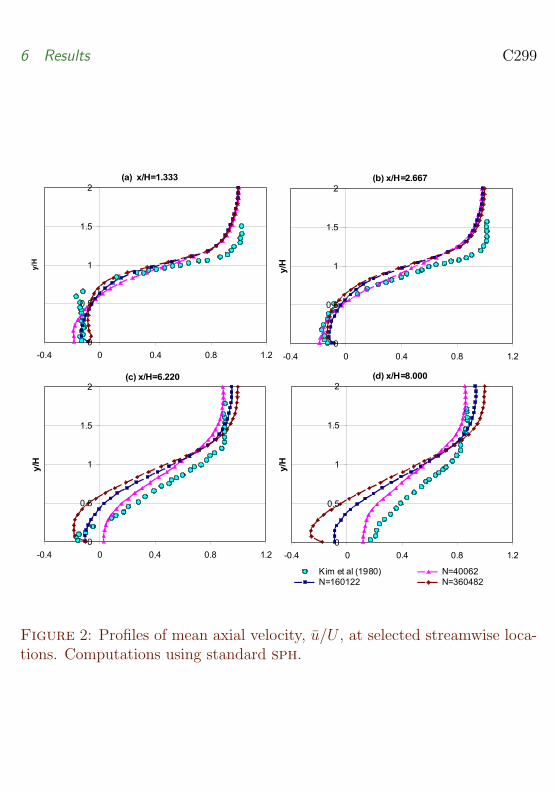