SIMULATION OF INERTIAL NAVIGATION SYSTEM ERRORS AT … · SIMULATION OF INERTIAL NAVIGATION SYSTEM ERRORS AT AERIAL PHOTOGRAPHY FROM UAV R. Shults. Kyiv National University of Construction

SIMULATION OF INERTIAL NAVIGATION SYSTEM ERRORS AT AERIAL

PHOTOGRAPHY FROM UAV

R. Shults

Kyiv National University of Construction and Architecture, Faculty for Geoinformation Systems and Territory Management,

Povitroflotskyi Avenue, 31 Kyiv, 03037, Ukraine, [email protected]

Commission V, WG V/7

KEY WORDS: Unmanned aerial vehicle, Aerial photography, Inertial navigation system (INS), Accelerometer systematic shift,

Gyroscope systematic offset, Position accuracy

ABSTRACT:

The problem of accuracy determination of the UAV position using INS at aerial photography can be resolved in two different ways:

modelling of measurement errors or in-field calibration for INS. The paper presents the results of INS errors research by

mathematical modelling. In paper were considered the following steps: developing of INS computer model; carrying out INS

simulation; using reference data without errors, estimation of errors and their influence on maps creation accuracy by UAV data. It

must be remembered that the values of orientation angles and the coordinates of the projection centre may change abruptly due to

the influence of the atmosphere (different air density, wind, etc.). Therefore, the mathematical model of the INS was constructed

taking into account the use of different models of wind gusts. For simulation were used typical characteristics of micro

electromechanical (MEMS) INS and parameters of standard atmosphere. According to the simulation established domination of INS

systematic errors that accumulate during the execution of photographing and require compensation mechanism, especially for

orientation angles. MEMS INS have a high level of noise at the system input. Thanks to the developed model, we are able to

investigate separately the impact of noise in the absence of systematic errors. According to the research was found that on the

interval of observations in 5 seconds the impact of random and systematic component is almost the same. The developed model of

INS errors studies was implemented in Matlab software environment and without problems can be improved and enhanced with new

blocks.

1. INTRODUCTION

The last 25 years in the world, we have seen a stable increase in

requirements for geospatial data. These requirements differ but

generally this is desire to improve the accuracy and detail of

data collection and at the same time increasing the speed and

reducing cost. In the traditional version with the aim of

mapping and GIS projects data were collected using traditional

methods of terrestrial survey or aerial photography. Terrestrial

technologies are complex and energy-intensive and not very

suitable for fast and detailed data collection and updating. On

the other hand, the traditional aerial photography with long

distance from the camera to the object does not allow

completely display all its characteristics, and the results are

highly dependent on weather conditions. Both technologies are

expensive and therefore not very suitable for frequent data

updates. Today, very popular is method of data collection using

GNSS (global navigation satellite system). However, this

method is actually a continuation of traditional terrestrial

survey because it requires direct determination of each point,

although however slightly reducing the cost of work and time

spent on data collection.

An alternative to existing methods of data collection is the use

of technology, which in complex use different navigation

technologies and remote sensing (Bosak, 2014). These

technologies include aerial photography using unmanned aerial

vehicles (UAV). The main advantage of this technology is the

simultaneous reduction of cost and time for data collection. In

comparison with aerial photography, UAV camera equipment is

much simpler, the surveying distances are smaller and the

efficiency is much higher (Colomina et al. 2014). Of course,

aerial photography from the UAVs has its drawbacks, such as

low accuracy at high altitudes. However, in many projects UAV

benefits are more significant in comparison with disadvantages.

Aerial photography from the UAVs provides the accuracy that

requires the most of the topographical work. However,

achieving the required level of accuracy is challenging. The

main problems in obtaining accurate data are concern to

navigation facilities as UAV navigation unit is a complex

system with many sensors that have completely different nature

of information. UAV navigation equipment may include GNSS,

barometric sensor, magnetic compass, tilt sensor, gyroscopes

system, accelerometers systems, INS. The best solution for

aerial photography using UAVs is navigation unit GNSS/INS.

Due to the high cost and bulkiness of accurate inertial

navigation systems for UAV are used miniature

electromechanical navigation systems (MEMS). These INSs

have undeniable advantages from the point of cost and

dimensions. However, the accuracy of inertial systems wishes

to better. Accelerometers and gyroscopes that are part of the

miniature navigation systems have low measurement accuracy.

Since determination of the position and orientation in space,

using INS based on double integration of the measured

accelerations and angular velocities, even minor errors at the

beginning of integration growing very quickly over time. For

INS errors correction are using two approaches:

- The study of a particular model of INS and construction

of mathematical dependencies, which describe system errors.

- INS correction at specified intervals, using GNSS data.

The first approach is suitable for high precision, tactical-grade

INS for which errors are stable and do not change over time.

INS of this type cannot be used for UAV due to high cost and

The International Archives of the Photogrammetry, Remote Sensing and Spatial Information Sciences, Volume XLII-1/W1, 2017 ISPRS Hannover Workshop: HRIGI 17 – CMRT 17 – ISA 17 – EuroCOW 17, 6–9 June 2017, Hannover, Germany

This contribution has been peer-reviewed. doi:10.5194/isprs-archives-XLII-1-W1-345-2017 345

huge weight. For low-cost INS rational is use of GNSS for

periodic correction (Abdel-Hamid, 2005; Grejner-Brzezinska, et

al. 2004) rather than calibration (Artese et al. 2008), due to

large and unstable errors. The choice of the interval by which

INS correction is performed depends on how quickly

accumulating errors and changing accuracy of INS in intervals

between corrections. Finally, from this depends the accuracy

with which the position of the UAV and the position and

orientation of aerial equipment will be determined (Rehak et al.,

2014). So, important is the task of INS errors simulation and

based on such research, setting INS correction interval using

GNSS. Such researches will allow choosing INS with proper

characteristics. Therefore, the main idea of this paper is

practical research of low-cost INS accuracy by mathematical

simulation results. Based on these results we tried to establish

the influence of INS position on accuracy of topographic maps

creation.

First of all we have to establish the mathematical model of INS.

2. INS MODEL

The main coordinate systems, which are using in inertial

navigation, are inertial system (i-system), earth centered system

(e-system), local horizontal navigation system (n-system), body

coordinate system (b-system). The core description and

determination of these systems you can find in (Biezad , 1999;

Salytcheva, 2004).

The orientation of UAV can be determined by three angles (φ -

roll, θ - pitch, ψ - heading), which need for connection

between vectors in b-system and n-system at the same point in

space.

We chose the INS model in which the angles and coordinates

get in n-system. In such case, we introduce a short description

of this model according to (Zang, 2003).

The equations of position and orientation calculation in n-

system have the next form:

1

2

nn

n n b n n n n

b ie en

nn b b

bb ib in

D vr

v R a Ω Ω v γ

R R ω Ω

, (1)

where ωie = Earth rotation velocity

ba = measured accelerations vector in b-system

b

ibω = measured angular velocities vector in b-system

2 n n n

ie en Ω Ω v = vector corrections for influence of

Сoriolis and centrifugal accelerations

nγ = vector of acceleration of normal gravity

0 ω c

0 ; 0 ,

ω -ω s

ie

e n n e

ie ie e ie

e ie

B

B

Ω Ω R Ω

10 0

10 0

c

0 0 1

M H

N H B

D.

Rotation from b-system to n-system is describing by next

matrix:

cψcθ -sψcφ+cψsθsφ sψsφ+cψsθcφ

sψcθ cψcφ+sψsθsφ -cψsφ+sψsθcφ

-sθ cθsφ cθcφ

n

b

R, (2)

Rotation from n-system to e-system can be implemented

through the transition velocity:

ω

ω

ωtg

x

y

z

E

n

en

n nNen en

n

enE

v

N H

v

M H

v B

N H

Ω, (3)

where B, L, H = geodetic coordinates

vE, vN = east and north components of velocity

M, N = main radius of ellipsoid

Total rotation from e-system to n-system is describing by next

matrix:

s c s s c

s c 0

c c c s s

n

en

B L B L B

L L

B L B L B

Ω (4)

In expressions, superscript indicates the coordinate system in

which parameters are presented, and the bottom shows the

original system of coordinates. For angular velocities, lower

index indicates in respect of which two coordinate systems

occurs rotation.

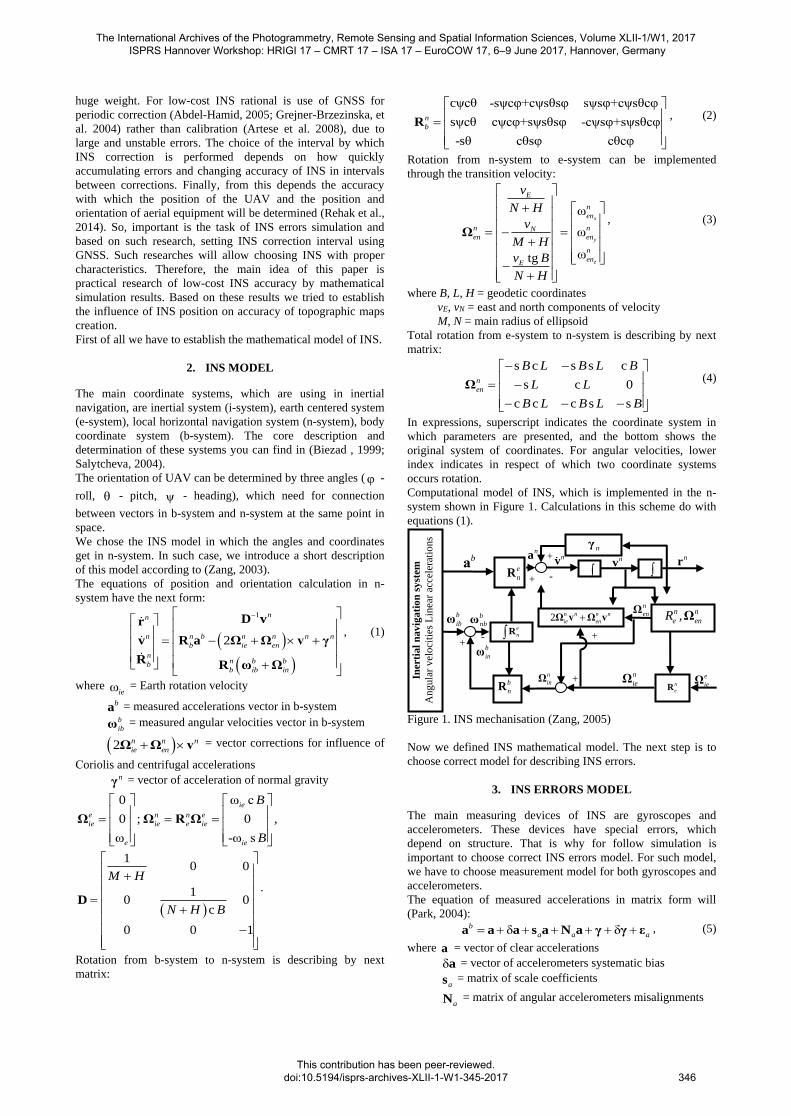
Computational model of INS, which is implemented in the n-

system shown in Figure 1. Calculations in this scheme do with

equations (1).

Figure 1. INS mechanisation (Zang, 2005)

Now we defined INS mathematical model. The next step is to

choose correct model for describing INS errors.

3. INS ERRORS MODEL

The main measuring devices of INS are gyroscopes and

accelerometers. These devices have special errors, which

depend on structure. That is why for follow simulation is

important to choose correct INS errors model. For such model,

we have to choose measurement model for both gyroscopes and

accelerometers.

The equation of measured accelerations in matrix form will

(Park, 2004):

δ δb

a a a a a a s a N a γ γ ε , (5)

where a = vector of clear accelerations

δa = vector of accelerometers systematic bias

as = matrix of scale coefficients

aN = matrix of angular accelerometers misalignments

Iner

tia

l n

av

iga

tion

sy

stem

An

gu

lar

vel

oci

ties

Lin

ear

acce

lera

tio

ns

b

ibω

bа

e

nR

nγ

нормальна

гравітація

,n n

e enR Ω b

nbω

na

b

inω

n

inΩ

nv

+ -

+

+ -

nv

b

nR n

eR

nr

2 n n n n

ie enΩ v Ω v n

enΩ

e

nR

+

+

n

ieΩ e

ieΩ


This contribution has been peer-reviewed. doi:10.5194/isprs-archives-XLII-1-W1-345-2017

346

γ = vector acceleration of normal gravity

δγ = vector of acceleration of normal gravity variations

aε = vector of accelerations measurements noise

Also, equation (5) in expanded form will:

δ ψ θ

δ ψ φ

δ θ φ

εγsinθ δγ

γcosθsinφ δγ ε .

γ cosθcosφ δγ ε

X

Y

Z

b

X X X X X

b

Y Y Y Y Y

b

Z Z Z Z Z

aX

Y a

Z a

a a a s a

a a a s a

a a a s a

The equation of measured angular velocities in matrix form

will:

ω ω ωδb

ib ω ω ω s ω N ω ε , (6)

where ω = vector of clear angular velocities

δω = vector of gyroscopes systematic bias

ωs = matrix of scale coefficients

ωN = matrix of angular gyroscopes misalignments

ωε = vector of gyroscopes measurements noise

Also, equation (6) in expanded form will:

Xω ω δω ψ θ ω ε

ω ω δω ψ φ ω ε .

ω ω δω θ φ ω ε

b

X X X X X

b

Y Y Y Y Y Y

b

Z Z Z Z Z Z

s

s

s

In the most cases, the random part is presented as a sum of

white noise and additional components.

ε ε ε ε ε ε ,W c r q t (7)

where εW = white noise

εc = correlation noise

εr = random shift

εq = quantization noise

ε t = trembling noise

The total errors model of random and systematic errors of

accelerometers and gyroscopes for simulation are possible to

present by equations (5) and (6) using devices specifications.

4. INITIAL DATA AND MATLAB SIMULINK MODEL

FOR SIMULATION

For our simulation, we need two types of initial data: technical

specifications of INS and simulated clear accelerations and

angular velocities. In order to construct errors model we chose

follow errors values (Goodall et al. 2012; Barret, 2014), which

presented in table below.

Error Value

Accelerometer bias δa 100 μg, 250 μg, 500 μg

Axis non-orthogonality 60"

Gyroscope bias δω 1,5°/hr, 2,5°/hr 5°/hr

Accelerometers noise, RMS 5 mg/ hr/√Hz

Gyroscopes noise, RMS 0.5°/hr/√Hz

Table 1. INS errors

According to large value of biases, the scale coefficients of

accelerometers and gyroscopes were neglected.

In the case of measured accelerations and angular velocities

were chosen three types of trajectories: straight spatial line,

classical surveying trajectory for one route (is using for linear

objects) and complicated curve, which has a form of “eight”

(often is using for INS calibration). All these trajectories

presented below.

Figure 2. Projection of spatial line on planes XOY and XOZ

Figure 3. Closed route along linear object

Figure 4. Complicated curve

The movement of UAV has taken uniform, with a constant

speed of 80 km / h. Using equations (1) the Matlab Simulink

model was created (Figure 5). The study was set up m-file,

which also ran simulations of two INS models, with the

influence of errors and without. During the simulation

automatically were formed at the same time the differences

between two position coordinates. The coordinate’s differences

were obtained for all three axes X, Y, Z. There were performed

27 launches of Matlab Simulink model. Nine launches were

made with the assumption that no error of gyroscopes. The

accelerometers errors consistently taken the values 100 μg, 250

μg, 500 μg. The next nine launches INS were made with the

assumption that no error of accelerometers. The gyroscopes

errors consistently take the values of 1.5°/h, 2.5°/h, 5°/h. One of

the aims of this research was to determine the effect separately



347

gyroscopes and accelerometers. The final option was executed

nine studies that included the presence of errors accelerometers

and gyroscopes.

Figure 5. Matlab Simulink model of INS

In this case were formed three errors models: first model (1) -

100 μg/1,5°/hr; second model (2) - 250 μg/2,5°/hr; third model

(3) - 500 μg/5°/hr. Other INS errors were left without changing

in all launches. The total time of simulation was 2 min.

Sampling frequency was 100 Hz.

5. INS SIMULATION RESULTS

Here we present the simulation results. The most comfortable is

presenting these results in graphic form. Due to lack of paper

volume, we are presenting just a little part of results. The

simpler interpretation of errors accumulation can be made for

trajectory of straight spatial line. Below presented the results of

errors accumulation along X axis.

Figure 6. Accelerometers errors accumulation along X axis

As we can see, in the modern MEMS INSs the level of errors is

too high. For distance 2 km, the displacement along X axis add

up to 1/8 from distance and grows by exponent.

Figure 7. Gyroscopes errors accumulation along X axis

Figure 8. Total errors accumulation along X axis

So, it is interesting to define in what time period the INS errors

will have accepted values. For this, we presented the graphics

of errors accumulation along Y axis for 2 seconds time interval.

As in the previous case, we are presenting displacements along

Y axis for three variants.



348

Figure 9. Accelerometers errors accumulation along Y axis

Figure 10. Gyroscopes errors accumulation along Y axis

Figure 11. Total errors accumulation along Y axis

From Figures 9-11, we can conclude that total errors of INS

have normal values. These results are very useful as allow

finding and establishing correct time interval for INS correction

by GNSS.

Another one useful property of constructed Matlab model is

possibility to research how the wind gusts can influence on

accuracy of position determination. Below presented such

simulations for model (1).

These results are quite interesting and need more dipper

analysis. Anyway, we can conclude that such atmosphere

phenomenon as wind gusts have significant influence on INS

accuracy.

Figure 12. Changing of INS error along X axis, including wind

gust

Figure 13. Changing of INS error along Y axis, including wind

gust

Figure 14. Changing of INS error along Z axis, including wind

gust

After this, the last step is results analysis

6. RESULTS ANALYSIS

To perform the analysis of the results we have to find out how

the errors of INS affecting on topographical maps accuracy.

In surveying assumed that if a source of error does not exceed

1/5 of the total value of the error, its influence is negligible. In

this case, we are considering the expected errors in scale of

aerial photographs. We can write:

δ δ δ1 1 1δ ; δ ; δ

5 5 5

INS INS INSX Y Z

x y p

p

m m H (8)

where δ ,δ ,δINS INS INSX Y Z

= coordinates determination errors

(from INS simulation)

δ ,δ ,δ δx y p z = errors of coordinates and parallaxes

measurements on image

m = image scale 4000 (for focus 50 mm and

surveying height 200 m)

p = parallax, 5 mm on image (for 80% overlap)

If we accept a scales of topographic maps 1:500, 1:1000,

1:2000, 1:5000, the error in determining the position will:



349

0.4δ ,δ

2X Y

M , (9)

where M = map scale.

For height we will have

1δ

3Z h , (10)

where h = vertical interval, which will take for these scales 0.5

m, 1.0 m, 1.0 m, 2.0 m.

Using the above value by expressions (9-10) we calculate the

acceptable points errors. Next, by the expressions (8) we

calculate the acceptable points errors on the image and points

errors on image due to errors INS for time interval of 2 seconds

(model 3). From the acceptable errors we move to values which

can be neglected and compare these values with INS errors.

Again, we will use simulation data for straight spatial line. The

calculation results are given in tables.

Scale Error on map

δX, m

Error on image δx,

mm ( 0.2δx mm)

INS error δINSX

on

image, mmк

500 0,14 0,035 (0,007) 0,013

1000 0,28 0,070 (0,014) 0,013

2000 0,57 0,140 (0,028) 0,013

5000 1,43 0,350 (0,070) 0,013

Table 2. Comparative analysis of calculated and acceptable INS

errors (axis X)

Scale Error on

map δY, m

Error on image δ y,

mm ( 0.2δ y mm)

INS error δINSY

on

image, mmк

500 0,14 0,035 (0,007) 0,016

1000 0,28 0,070 (0,014) 0,016

2000 0,57 0,140 (0,028) 0,016

5000 1,43 0,350 (0,070) 0,016


errors (axis Y)

Scale Error on

map δZ, m

Error on image δz,

mm ( 0.2δz mm)

INS error δINSZ

on

image, mmк

500 0,17 (0,5) 0,004 (0,0008) 0,0013

1000 0,33 (1,0) 0,008 (0,0016) 0,0013

2000 0,33 (1,0) 0,008 (0,0016) 0,0013

5000 0,67 (2,0) 0,017 (0,0032) 0,0013


errors (axis Z)

If we assume that GNSS works with frequency 1 Hz and can

determine the coordinates with precision 0,02-0,03 m in any

axis, then INS allows to determine with the necessary accuracy

the position of the UAV in the intervals between the GNSS-

measurements. On the observation interval of 2 seconds INS

can be used when creating topographical maps of scale 1: 1000.

7. CONCLUSIONS

In presented paper was constructed and investigated

mathematical model of INS errors. The research established the

dominance of systematic errors of INS that accumulate during

the performance of aerial photography from UAV and require

compensation mechanism, especially for orientation angles. It

was established that low cost INS have another characteristic

feature. This is the high level of noise at the system input.

Thanks to the model developed by us, we are able to examine

separately the impact of noise in the absence of systematic

errors.

The accuracy of INS was simulated for different operating time.

For the 5 seconds time interval was established that random and

systematic impact component is almost the same. Therefore,

when performing coordinates correction by GNSS, the

assessment of systematic component impact can be done only

on time intervals from 10 seconds. At the same time the rate of

accumulation of errors in angular orientation is slower. In this

case can be recommended to use the gyroscopes errors model.

The influence of wind gusts on INS coordinates were carried

out. These results need future investigations. One of the way in

which it can be done, it is using vehicle dynamic model as it

was made in paper (Khaghani et al., 2016).

At the end of a paper was given methodic of assessment INS

errors affecting on topographical maps accuracy. Therefore we

can assess the influence of INS errors and choose proper

navigation equipment.

REFERENCES

Abdel-Hamid, W., 2005. Accuracy Enhancement of Integrated

MEMS-IMU/GPS Systems for Land Vehicular Navigation

Applications. A Thesis for the Degree Doctor of Philosophy.

Calgary.

Artese, G., Trecroci A., 2008. Calibration of a low cost MEMS

INS sensor for an integrated navigation system. In: The

International Archives of the Photogrammetry, Remote Sensing

and Spatial Information Sciences, Beijing, China, Vol.

XXXVII, Part B5, pp. 877-882.

Barret, J.M., 2014. Analyzing and modeling low-cost MEMS

IMUs for use in an inertial navigation system. A Thesis for the

Degree of Master of Science. Worcester.

Biezad, D.J., 1999. Integrated Navigation and Guidance

Systems. American Institute of Aeronautics and Astronautics,

Reston, 242 p.

Bosak, K., 2014. Secrets of UAV photomapping

http://s3.amazonaws.com/DroneMapper_US/documentation/pte

ryx-mapping-secrets.pdf.

Colomina, I., Molina, P., 2014. Unmanned aerial systems for

photogrammetry and remote sensing: A review. ISPRS Journal

of Photogrammetry and Remote Sensing, Vol. 92, pp. 79–97.

dx.doi.org/10.1015/j.isprsjprs.2014.02.013.

Goodall, C., Carmichael, S., El-Sheimy, N., Scannell, B., 2012.

INS Face Off MEMS versus FOGs. InsideGNSS,

JULY/AUGUST, pp. 48-55.

Grejner-Brzezinska, D.A., Toth, C.K., 2004. High-Accuracy

Direct Aerial Platform Orientation with Tightly Coupled

GPS/INS System. Ohio Department of Transportation, Office of

Aerial Engineering, Federal Highway Administration.

Khaghani, M., Skaloud, J., 2016. Application of vehicle

dynamic modeling in UAVs for precise determination of

exterior prientation. In: The International Archives of the



350

http://s3.amazonaws.com/DroneMapper_US/documentation/pteryx-mapping-secrets.pdf

http://s3.amazonaws.com/DroneMapper_US/documentation/pteryx-mapping-secrets.pdf

Photogrammetry, Remote Sensing and Spatial Information

Sciences, Prague, Czech Republic, Vol. XLI-B3, pp. 827-831.

Park, M., 2004. Error Analysis and Stochastic Modeling of

MEMS based Inertial Sensors for Land Vehicle Navigation

Applications. A Thesis for the Degree Doctor of Philosophy.

Calgary

Rehak, M., Mabillard, R., Skaloud, J., 2014. A Micro Aerial

Vehicle with Precise Position and Attitude Sensors. PFG

Photogrammetrie, Fernerkundung, Geoinformation, Issue 4, pp.

239-251, DOI: 10.1127/1432-8364/2014/0240

Salytcheva, A.O., 2004. Medium Accuracy INS/GPS

Integration in Various GPS Environments. A Thesis for the

Degree of Master of Science. Calgary.

Shin, E.-H., 2005. Estimation Techniques for Low Cost Inertial

Navigation. A Thesis for the Degree Doctor of Philosophy.

Calgary.

Zang, Z., 2003. Integration of GPS with A Medium Accuracy

IMU for Metre-Level Positioning. A Thesis for the Degree of

Master of Science. Calgary.

Revised April 2017


This contribution has been peer-reviewed. doi:10.5194/isprs-archives-XLII-1-W1-345-2017 351

https://www.schweizerbart.de/papers/pfg/detail/2014/84307/A_Micro_Aerial_Vehicle_with_Precise_Position_and_Attitude_Sensors

https://www.schweizerbart.de/papers/pfg/detail/2014/84307/A_Micro_Aerial_Vehicle_with_Precise_Position_and_Attitude_Sensors

Documents

SIMULATION OF INERTIAL NAVIGATION SYSTEM ERRORS AT … · SIMULATION OF INERTIAL NAVIGATION SYSTEM ERRORS AT AERIAL PHOTOGRAPHY FROM UAV R. Shults. Kyiv National University of Construction