Simulation of Vehicle Working Conditions with Hydrostatic ...yadda.icm.edu.pl/yadda/element/bwmeta1.element.baztech-article-BU… · Simulation of Vehicle Working Conditions with

Journal of Automation, Mobile Robotics & Intelligent Systems VOLUME 6, N° 3 2012

Articles40

Simulation of Vehicle Working Conditions

with Hydrostatic Pump and Motor Control Algorithm

Peter Zavadinka, Peter Kriššák

Submitted 26th June 2011; accepted 16thSeptember 2011

Abstract: Emission rules have significant impact on market of

mobile working machines. They bring new challenges for transmission, working, controlling and vehicle manage-ment functions. Extensive knowledge from design, control system, optimization, automation, signal processing, sys-tem modeling etc. are welcome to get answer how best to produce more efficient, productive machines. In case of new concepts is appropriate to create complex dynamic model of machine. Presented paper describes a four wheel drive model and simulation of a mobile working machine and the concept of hydrostatic pump and motor control al-gorithm in selected conditions.

Keywords: hydrostatic pump and motor, control algo-rithm, mobile working machine, energy savings

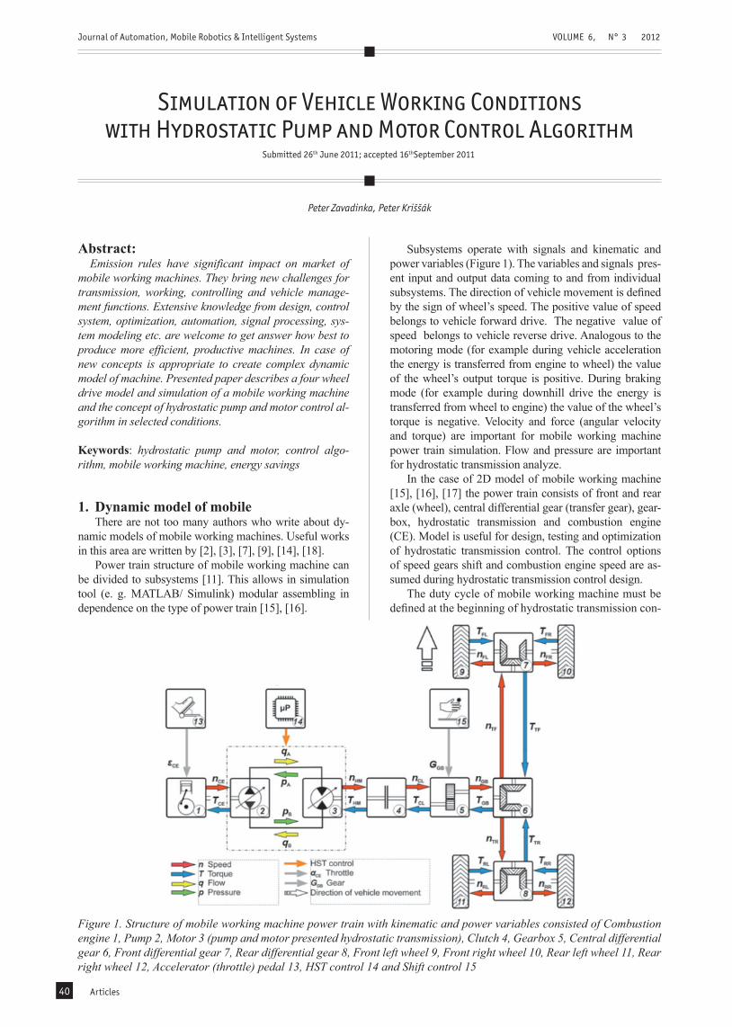
Subsystems operate with signals and kinematic and power variables (Figure 1). The variables and signals pres-ent input and output data coming to and from individual subsystems. The direction of vehicle movement is defined by the sign of wheel’s speed. The positive value of speed belongs to vehicle forward drive. The negative value of speed belongs to vehicle reverse drive. Analogous to the motoring mode (for example during vehicle acceleration the energy is transferred from engine to wheel) the value of the wheel’s output torque is positive. During braking mode (for example during downhill drive the energy is transferred from wheel to engine) the value of the wheel’s torque is negative. Velocity and force (angular velocity and torque) are important for mobile working machine power train simulation. Flow and pressure are important for hydrostatic transmission analyze.

In the case of 2D model of mobile working machine [15], [16], [17] the power train consists of front and rear axle (wheel), central differential gear (transfer gear), gear-box, hydrostatic transmission and combustion engine (CE). Model is useful for design, testing and optimization of hydrostatic transmission control. The control options of speed gears shift and combustion engine speed are as-sumed during hydrostatic transmission control design.

The duty cycle of mobile working machine must be defined at the beginning of hydrostatic transmission con-

1. Dynamic model of mobileThere are not too many authors who write about dy-

namic models of mobile working machines. Useful works in this area are written by [2], [3], [7], [9], [14], [18].

Power train structure of mobile working machine can be divided to subsystems [11]. This allows in simulation tool (e. g. MATLAB/ Simulink) modular assembling in dependence on the type of power train [15], [16].

Figure 1. Structure of mobile working machine power train with kinematic and power variables consisted of Combustion engine 1, Pump 2, Motor 3 (pump and motor presented hydrostatic transmission), Clutch 4, Gearbox 5, Central differential gear 6, Front differential gear 7, Rear differential gear 8, Front left wheel 9, Front right wheel 10, Rear left wheel 11, Rear right wheel 12, Accelerator (throttle) pedal 13, HST control 14 and Shift control 15


Articles 41

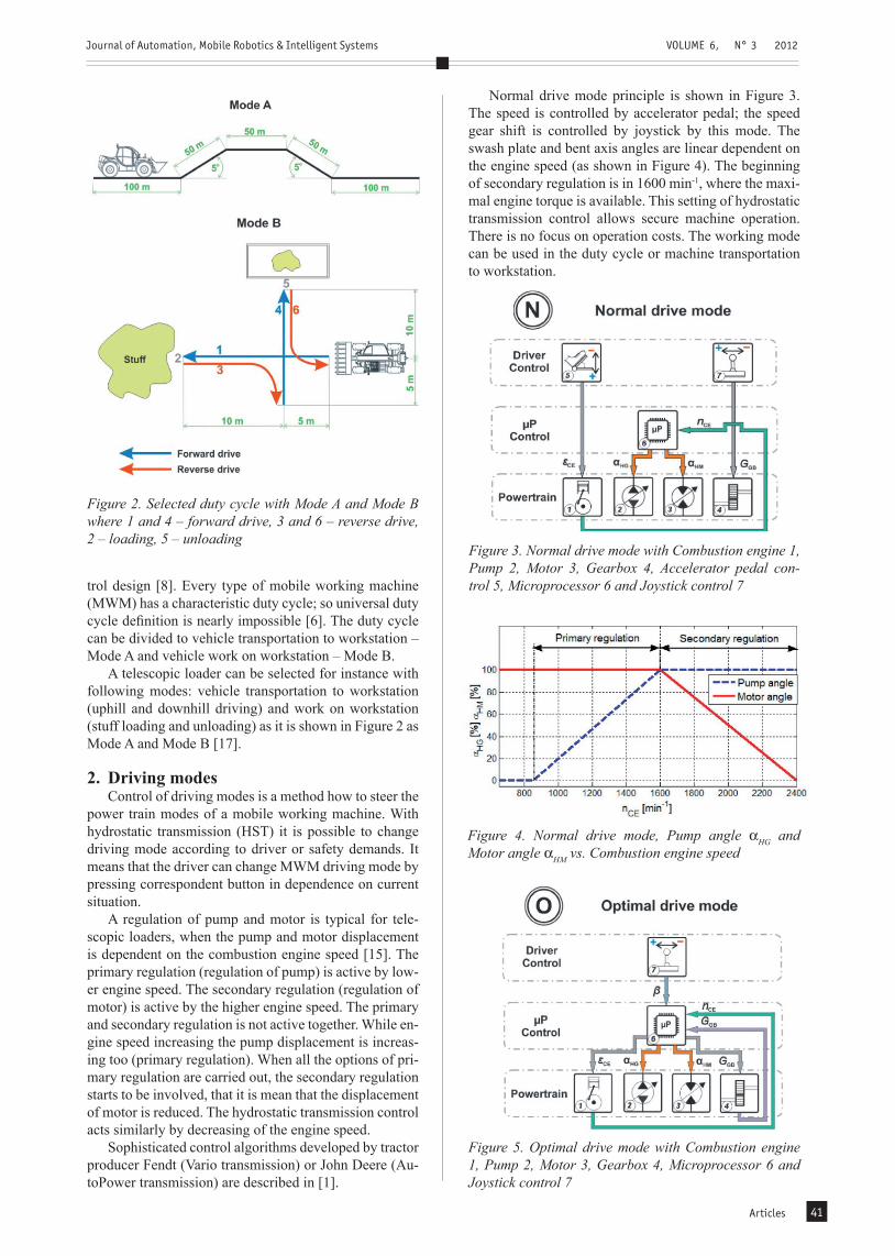
trol design [8]. Every type of mobile working machine (MWM) has a characteristic duty cycle; so universal duty cycle definition is nearly impossible [6]. The duty cycle can be divided to vehicle transportation to workstation – Mode A and vehicle work on workstation – Mode B.

A telescopic loader can be selected for instance with following modes: vehicle transportation to workstation (uphill and downhill driving) and work on workstation (stuff loading and unloading) as it is shown in Figure 2 as Mode A and Mode B [17].

2. Driving modesControl of driving modes is a method how to steer the

power train modes of a mobile working machine. With hydrostatic transmission (HST) it is possible to change driving mode according to driver or safety demands. It means that the driver can change MWM driving mode by pressing correspondent button in dependence on current situation.

A regulation of pump and motor is typical for tele-scopic loaders, when the pump and motor displacement is dependent on the combustion engine speed [15]. The primary regulation (regulation of pump) is active by low-er engine speed. The secondary regulation (regulation of motor) is active by the higher engine speed. The primary and secondary regulation is not active together. While en-gine speed increasing the pump displacement is increas-ing too (primary regulation). When all the options of pri-mary regulation are carried out, the secondary regulation starts to be involved, that it is mean that the displacement of motor is reduced. The hydrostatic transmission control acts similarly by decreasing of the engine speed.

Sophisticated control algorithms developed by tractor producer Fendt (Vario transmission) or John Deere (Au-toPower transmission) are described in [1].

Normal drive mode principle is shown in Figure 3. The speed is controlled by accelerator pedal; the speed gear shift is controlled by joystick by this mode. The swash plate and bent axis angles are linear dependent on the engine speed (as shown in Figure 4). The beginning of secondary regulation is in 1600 min-1, where the maxi-mal engine torque is available. This setting of hydrostatic transmission control allows secure machine operation. There is no focus on operation costs. The working mode can be used in the duty cycle or machine transportation to workstation.

Figure 2. Selected duty cycle with Mode A and Mode B where 1 and 4 – forward drive, 3 and 6 – reverse drive, 2 – loading, 5 – unloading

Figure 3. Normal drive mode with Combustion engine 1, Pump 2, Motor 3, Gearbox 4, Accelerator pedal con-trol 5, Microprocessor 6 and Joystick control 7

Figure 5. Optimal drive mode with Combustion engine 1, Pump 2, Motor 3, Gearbox 4, Microprocessor 6 and Joystick control 7

Figure 4. Normal drive mode, Pump angle αHG and Motor angle αHM vs. Combustion engine speed


Articles42

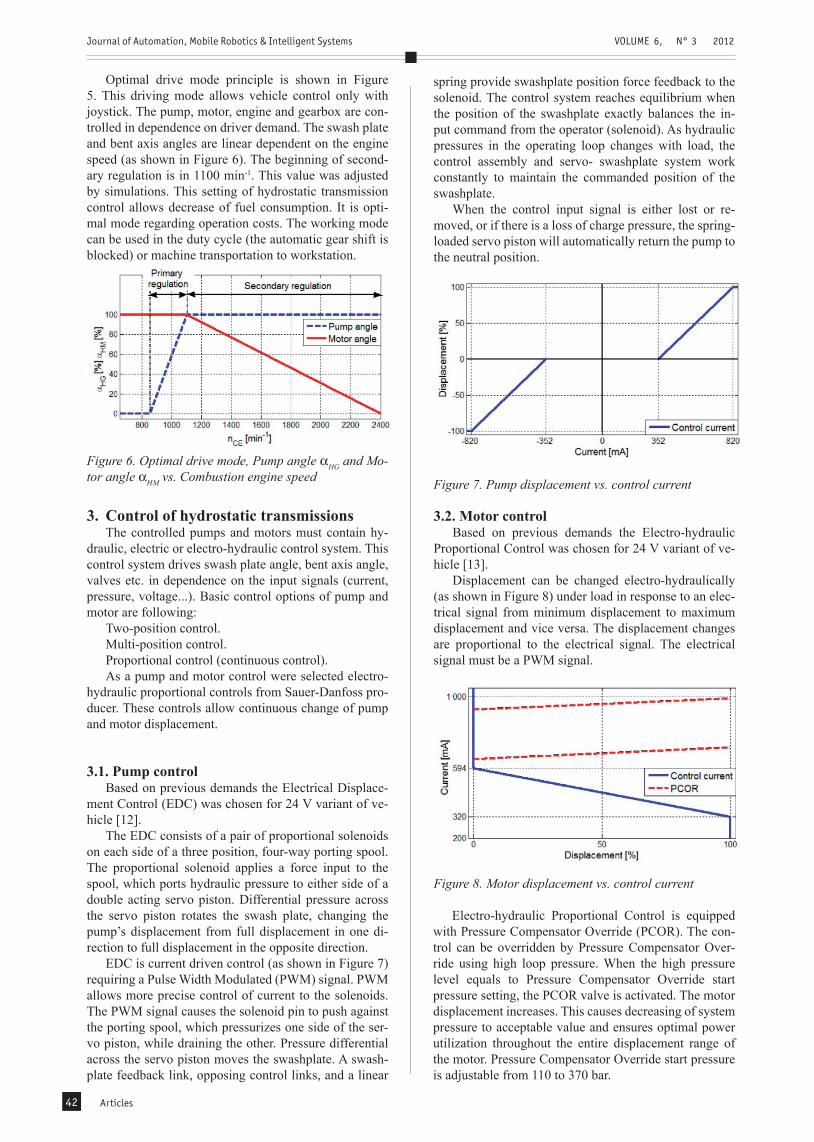
Optimal drive mode principle is shown in Figure 5. This driving mode allows vehicle control only with joystick. The pump, motor, engine and gearbox are con-trolled in dependence on driver demand. The swash plate and bent axis angles are linear dependent on the engine speed (as shown in Figure 6). The beginning of second-ary regulation is in 1100 min-1. This value was adjusted by simulations. This setting of hydrostatic transmission control allows decrease of fuel consumption. It is opti-mal mode regarding operation costs. The working mode can be used in the duty cycle (the automatic gear shift is blocked) or machine transportation to workstation.

Figure 6. Optimal drive mode, Pump angle αHG and Mo-tor angle αHM vs. Combustion engine speed

3. Control of hydrostatic transmissionsThe controlled pumps and motors must contain hy-

draulic, electric or electro-hydraulic control system. This control system drives swash plate angle, bent axis angle, valves etc. in dependence on the input signals (current, pressure, voltage...). Basic control options of pump and motor are following:

Two-position control.Multi-position control.Proportional control (continuous control).As a pump and motor control were selected electro-

hydraulic proportional controls from Sauer-Danfoss pro-ducer. These controls allow continuous change of pump and motor displacement.

3.1. Pump controlBased on previous demands the Electrical Displace-

ment Control (EDC) was chosen for 24 V variant of ve-hicle [12].

The EDC consists of a pair of proportional solenoids on each side of a three position, four-way porting spool. The proportional solenoid applies a force input to the spool, which ports hydraulic pressure to either side of a double acting servo piston. Differential pressure across the servo piston rotates the swash plate, changing the pump’s displacement from full displacement in one di-rection to full displacement in the opposite direction.

EDC is current driven control (as shown in Figure 7) requiring a Pulse Width Modulated (PWM) signal. PWM allows more precise control of current to the solenoids. The PWM signal causes the solenoid pin to push against the porting spool, which pressurizes one side of the ser-vo piston, while draining the other. Pressure differential across the servo piston moves the swashplate. A swash-plate feedback link, opposing control links, and a linear

spring provide swashplate position force feedback to the solenoid. The control system reaches equilibrium when the position of the swashplate exactly balances the in-put command from the operator (solenoid). As hydraulic pressures in the operating loop changes with load, the control assembly and servo- swashplate system work constantly to maintain the commanded position of the swashplate.

When the control input signal is either lost or re-moved, or if there is a loss of charge pressure, the spring-loaded servo piston will automatically return the pump to the neutral position.

Figure 7. Pump displacement vs. control current

3.2. Motor controlBased on previous demands the Electro-hydraulic

Proportional Control was chosen for 24 V variant of ve-hicle [13].

Displacement can be changed electro-hydraulically (as shown in Figure 8) under load in response to an elec-trical signal from minimum displacement to maximum displacement and vice versa. The displacement changes are proportional to the electrical signal. The electrical signal must be a PWM signal.

Figure 8. Motor displacement vs. control current

Electro-hydraulic Proportional Control is equipped with Pressure Compensator Override (PCOR). The con-trol can be overridden by Pressure Compensator Over-ride using high loop pressure. When the high pressure level equals to Pressure Compensator Override start pressure setting, the PCOR valve is activated. The motor displacement increases. This causes decreasing of system pressure to acceptable value and ensures optimal power utilization throughout the entire displacement range of the motor. Pressure Compensator Override start pressure is adjustable from 110 to 370 bar.


Articles 43

Electro-hydraulic Proportional Control should be equipped with Hydraulic Brake Pressure Defeat system or Electric Brake Pressure Defeat system.

4. Control algorithm model of hydrostatic unitsThe developed hydrostatic transmission control is

based on the previously mentioned driving modes. In the normal driving mode vehicle speed is controlled by accelerator pedal. The demanded engine speed is output from control block (subsystem) to combustion engine. The engine speed feedback is used for displacement con-trol of pump and motor (as shown in Figure 3). A shift of speed gear upwards is realized with forward joystick movement and a shift of speed gear downwards is real-ized with reverse joystick movement.

The optimal drive mode operates like a normal mode but with two differences. First difference is in the way how the vehicle speed (Combustion engine speed) is set. The speed in the optimal mode is controlled by joystick. The swash plate angle and bent axis angle dependence on the engine speed is shown in Figure 5. Second difference is automatic speed gear shift in the optimal drive mode. The automatic speed gear shift is dependent on the en-gine speed analogous to pump and motor displacement. It can be switched off.

Both drive modes are prepared to reversal drive and braking with hydrostatic transmission. During reversal drive the displacement of pump is opposite. The devel-oped model of hydrostatic transmission control is de-scribed in [16].

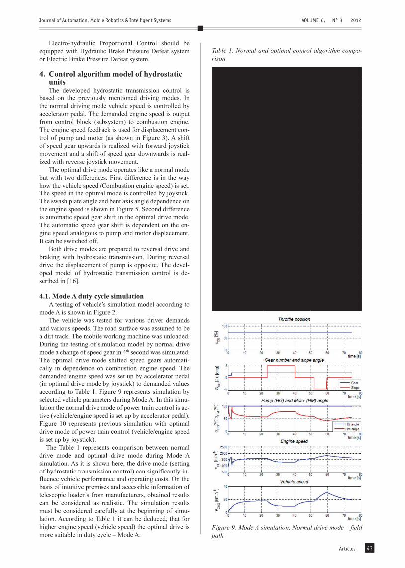
4.1. Mode A duty cycle simulationA testing of vehicle’s simulation model according to

mode A is shown in Figure 2.The vehicle was tested for various driver demands

and various speeds. The road surface was assumed to be a dirt track. The mobile working machine was unloaded. During the testing of simulation model by normal drive mode a change of speed gear in 4th second was simulated. The optimal drive mode shifted speed gears automati-cally in dependence on combustion engine speed. The demanded engine speed was set up by accelerator pedal (in optimal drive mode by joystick) to demanded values according to Table 1. Figure 9 represents simulation by selected vehicle parameters during Mode A. In this simu-lation the normal drive mode of power train control is ac-tive (vehicle/engine speed is set up by accelerator pedal). Figure 10 represents previous simulation with optimal drive mode of power train control (vehicle/engine speed is set up by joystick).

The Table 1 represents comparison between normal drive mode and optimal drive mode during Mode A simulation. As it is shown here, the drive mode (setting of hydrostatic transmission control) can significantly in-fluence vehicle performance and operating costs. On the basis of intuitive premises and accessible information of telescopic loader’s from manufacturers, obtained results can be considered as realistic. The simulation results must be considered carefully at the beginning of simu-lation. According to Table 1 it can be deduced, that for higher engine speed (vehicle speed) the optimal drive is more suitable in duty cycle – Mode A.

Table 1. Normal and optimal control algorithm comparison

NORMAL DRIVE MODE

Demanded CE speed [min-1]

Fuel consump-tion [l]

Range time [s]

1500 0.1610 280.5

1800 0.1322 150.3

2000 0.1216 98.4

2200 0.1246 61.6

OPTIMAL DRIVE MODE


Fuel consump-tion [l]

Range time [s]

1500 0.1874 398.0

1800 0.1141 110.6

2000 0.1150 77.1

2200 0.1083 51.5

OPTIMAL vs. NORMAL DRIVE MODE


Fuel consumption [%]

Range time [%]

1500 +16.4 +41.9

1800 -13.7 -26.4

2000 -5.4 -21.6

2200 -13.1 -16.4

Figure 9. Mode A simulation, Normal drive mode – field path


Articles44

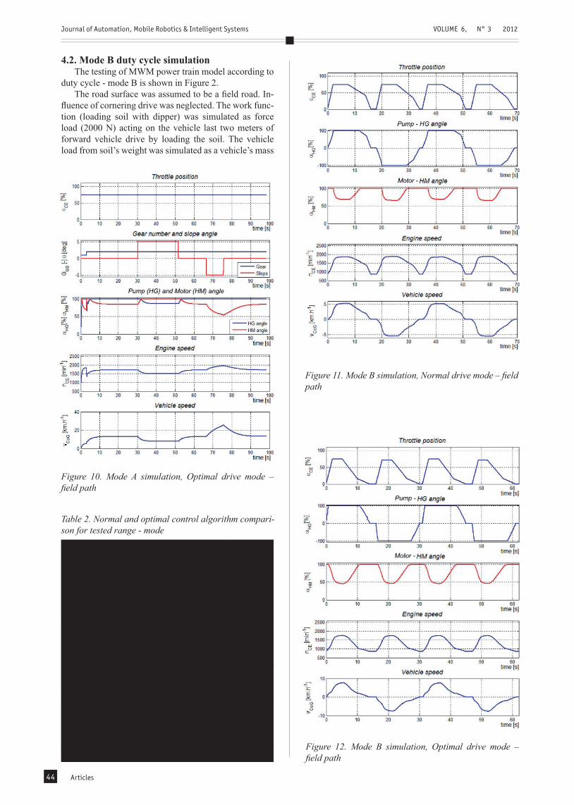
4.2. Mode B duty cycle simulationThe testing of MWM power train model according to

duty cycle - mode B is shown in Figure 2.The road surface was assumed to be a field road. In-

fluence of cornering drive was neglected. The work func-tion (loading soil with dipper) was simulated as force load (2000 N) acting on the vehicle last two meters of forward vehicle drive by loading the soil. The vehicle load from soil’s weight was simulated as a vehicle’s mass

Table 2. Normal and optimal control algorithm compari-son for tested range - mode

NORMAL DRIVE MODE

Loading resistance [N], Load [kg], Fuel consumption [l]

Range time [s]

2000 (13m-15m), 500 (15m-45m), 0.0356 70

OPTIMAL DRIVE MODE

Loading resistance [N], Load [kg], Fuel consumption [1]

Range time [s]

2000 (13m-15m), 500 (15m-45m), 0.0276 62

OPTIMAL vs NORMAL DRIVE MODE

Loading resistance [N], Load [kg], Fuel consumption [%]

Range time [%]

2000 (13m-15m), 500 (15m-45m), -22.5 -11.4

Figure 10. Mode A simulation, Optimal drive mode – field path

Figure 11. Mode B simulation, Normal drive mode – field path

Figure 12. Mode B simulation, Optimal drive mode – field path


Articles 45

increase (+500 kg) from the moment of loading till un-loading as illustrated in Figure 2. During the simulation the first speed gear was engaged. The demanded com-bustion engine speed was set up by accelerator pedal (in optimal drive mode by joystick). The maximal demanded value of the combustion engine speed was 2000 min-1. The characteristic of demanded combustion engine speed was set up so that the vehicle could drive required dis-tance without using mechanical brakes.

The results of simulation for Mode B and normal drive mode (combustion engine speed is set up by accelerator pedal) are shown in Figure 11. The Figure 12 represents results of the same test but for optimal drive mode (com-bustion engine speed is set up by joystick).

Analogous to previous tests obtained results can be considered as realistic (with respect to used parameters and equations). The test results must be again considered carefully at the beginning of simulation. An influence of the loading and weight increase was minimal. The differ-ences can be detected only by detailed search.

The Table 2 represents comparison between normal drive mode and optimal drive mode during Mode B sim-ulation. Drive mode (setting of hydrostatic transmission control) again significantly influenced simulation results. The loading with enabled optimal drive mode significant-ly decreased fuel consumption and loading cycle time.

5. ConclusionsIn this paper the simulation model of four wheel ve-

hicle power train with control algorithm was presented.Individual subsystems in model: combustion engine,

hydrostatic transmission, gearbox, central differential gear, wheels, vehicle chassis and control were modeled separately by blocks. Modular structure increased speed and efficiency of mobile working machine power train modeling. The individual blocks were created in MAT-LAB-Simulink program. A model of each subsystem (block) was equipped with mask, what increased user’s comfort of parameters setting.

Detailed modeling of subsystem dynamics is difficult and imprecise because of model complexity and difficul-ties by acquiring of some parameters. For example the tire modeling is one of the most difficult fields of ve-hicle’s modeling nowadays. Almost all modeled subsys-tems are non-linear.

The developed model shows strong non-linear behav-ior, which decelerates simulation mainly at the beginning.

The designed linear control algorithm shows relative-ly promising results. But it is still only base conception of the control algorithm. All performed simulations show acceptable results however in some cases (start, gear shift) it is necessary to consider physical and mathemati-cal complexity of model’s structure. During the simula-tion, it is important to know relationships and principles behind the user interface of these blocks; otherwise the simulation results can be misinterpreted by the engineer.

All performed simulations show acceptable results however in some cases (start, gear shift) it is necessary to consider physical and mathematical complexity of model’s structure. During the simulation, it is important to know relationships and principles behind the user in-terface of these blocks, otherwise the simulation results can be misinterpreted.

Developed models of subsystem contain some op-tions, whose using is not confirmed yet. The tendency of this application settings results from need of including the inertia during acceleration.

Despite of this we can assume that the reduction of fuel consumption can be done by suitable modification of pump and motor control characteristics. It can be de-duced, that the hydrostatic transmission setting in the optimal drive is more suitable. For selected application and testing cycles the using of primary regulation is more suitable for lower engine speed and smaller speed range.

In the future, it is necessary to continue with develop-ing of new blocks of drive and control and also with de-bugging of the initial conditions and parameter settings. Many of these were only guessed because of unavail-ability. This work provides good base for further model development of mobile working machine.

AUTHORS

Peter Zavadinka* – Ustav mechaniky teles, mechatron-iky a biomechaniky, Fakulta strojniho inzenyrstvi, VUT v Brne, Technicka 2896/2, 616 69 Brno, Czech Republic, [email protected]

Peter Krissak* – Technical centre, Sauer-Danfoss a.s., Kukucinova 2148-84, 017 01 Povazska Bystrica, Slovak Republic, [email protected]

* Corresponding author

References

[1] Bauer F., Sedlak P., & Smerda, T., Traktory. Praha: Prori Press, 2006.

[2] Carlsson E., Modeling Hydrostatic Transmission in Forest Vehicle. M.S. Linkopings Universitet, 2006.

[3] Carter D., Load modeling and emulation for an earthmoving vehicle power train. M.S. University of Illinois at Urbana-Champaign, 2003.

[4] Carter D. E., Alleyne A. G., “Earthmoving vehicle power train controller design and evaluation”. In: Proceedings of the American Control Conference, 30thJune 2004- 2nd July 2004, pp. 4455-4460.

[5] Grepl R., “Real-Time Control Prototyping in MAT-LAB/Simulink: Review of tools for research and education in mechatronics”. In: IEEE International Conference on Mechatronics (ICM 2011), 13th-15th April 2011, Istanbul, Turkey.

[6] Grepl R., Vejlupek J., Lambersky V., Jasansky M., Vadlejch F., Coupek P., “Development of 4WS/4WD Experimental Vehicle: platform for research and education in mechatronics”. In: IEEE International Conference on Mechatronics (ICM 2011), 13th-15th April 2011, Istanbul, Turkey.

[7] Kiencke U., Nielsen L.,: Automotive Control Sys-tems: For Engine, Driveline, and Vehicle. 2nd ed., Springer-Verlag: Germany, 2005.

[8] Kriššák P., Kučík P., “Computer aided measure-ment of hydrostatic transmission characteristics”,


Articles46

Hydraulika i Pneumatyka, 4/2005, p. 22-25, INDEX 37726, ISSN 1505-3954.

[9] Prasetiawan E., Modeling, simulation and control of an earthmoving vehicle power train simulator. M.S. University of Illinois at Urbana-Champaign, 2001.

[10] Rill G., Vehicle dynamics: Lecture notes. [Online] Regensburg: University of applied sciences, 2007, Available at: http:// homepages.fh-regensburg.de/~rig39165/skripte/ Vehicle_ Dynamics.pdf [Accessed 27 October 2008].

[11] Rill G., “Vehicle modeling by subsystems”, Jour-nal of the Brazilian Society of Mechanical Sciences and Engineering, [Online]. vol. 28, no. 4, 2006, p. 430-442. Available at: http://www.scielo.br/scielo.php?pid=S1678-58782006000400007&script=sci_arttext&tlng=en [Accessed 9 January 2010].

[12] Sauer-Danfoss: H1 Axial Piston Pumps 045/053 Single, 045/053 Tandem, 018 Single, 115/130 Sin-gle, 147/165 Single, 2009. [Online] Sauer-Danfoss. Available at: http://www.sauer-danfoss.com/stel-lent/groups/publications/ documents/product_lit-erature/ 11009999.pdf [Accessed 27 March 2009].

[13] Sauer-Danfoss: Series 51, Series 51-1, Bent Axis Variable Displacement Motors, Technical Infor-mation, 2003. [Online] Sauer-Danfoss. Avail-able at: http://www.sauer-danfoss.com/stellent/groups/ publications/documents/product_litera-ture/52010440.pdf [Accessed 15 February 2009].

[14] Tinker M., Wheel loader power train modeling for real-time vehicle. M.S. University of Iowa, 2006.

[15] Zavadinka P., Krissak P., Modeling and simulation of diesel engine for mobile working machine power train. In: Polish Society of Mechanical Engineers and Technicians - SIMP. Hydraulics and Pneumat-ics 2009: Domestic branch and turbulent global market. Wrocław, Poland 7-9 October 2009. SIMP: Wroclaw, Poland, 2009, ISBN 978-83-87982-34-8, pp. 339-348.

[16] Zavadinka P., Modeling and Simulation of Mobile Working Machine Power train. M.S. Brno Univer-sity of Technology, 2009.

[17] Zavadinka P., Kriššák P., Modeling and simulation of mobile working machine power train. In: Tech-nical Computing Prague 2009, 19.11.2009, Praha, Česká republika, 2009, p. 118, ISBN 978-80-7080-733-0.

[18] Zhang, R.: Multivariable robust control of non-linear systems with application to an electro- -hydraulic power train. Ph.D. University of Illinois at Urbana-Champaign, 2002.

[19] Zhang R., Alleyne, A. G. Carter D. E., “Robust gain scheduling control of an earthmoving vehicle power train”. In: Proceedings of the American Con-trol Conference, 2003, vol. 6, no. 4-6, June 2003, pp. 4969- 4974.

Documents

Simulation of Vehicle Working Conditions with Hydrostatic ...yadda.icm.edu.pl/yadda/element/bwmeta1.element.baztech-article-BU… · Simulation of Vehicle Working Conditions with