Embed Size (px)
Citation preview
SIMULTANEOUS MODULAR CONCEPT
IN CHEMICAL PROCESS SIMULATION AND OPTIMIZATION
by
RODRIGO ANTONIO TREVINO-LOZANO
B. S. University of Wisconsin, Madison(1979)
S.M. Massachusetts Institute of Technology(1981)
Submitted to the Department ofChemical Engineering
in Partial Fulfillment of the
Requirements of the Degree of
DOCTOR OF PHILOSOPHY
at the
MASSACHUSETTS INSTITUTE OF TECHNOLOGY
January 1985
Rodrigo Antonio Trevino-Lozano 1985
The Author hereby grants to M.I.T. permission to reproduce and todistribute copies of this thesis document in whole or in part.
Signature of the Author:
Certified by:
SiAccepted by:
Signature RedactedDeparftent of Chemical Engineering
To ",,. ," r . 1 10R %
Signature Redacted
Lawrence B. EvansThesis Supervisor
gnature RedactedRobert C. Reid
Chairman, Department Graduate Committee
MASSACHUSETTS iNSTITUTEOF TECHNOLOGY
ARCHIVES
LI8RANES
FEB 13 1985

-2-
Simultaneous Modular Concept
in Chemical Process Simulation and Optimization
by
Rodrigo Antonio Trevino-Lozano
Submitted to the Department of Chemical Engineering in January, 1985
in partial fulfillment of the requirements for the degree of Doctor of
Philosophy from the Massachusetts Institute of Technology.
ABSTRACT
This thesis presents the results of a prototype implementation of
a simultaneous modular algorithm for flowsheet simulation and
optimization in an industrial simulator environment. The ASPEN PLUS
process simulation system was used as the basis for a research project
aimed at developing and evaluating a "two-tier" simultaneous modular
algorithm to converge and optimize flowsheets. A wide variety of unit
operation blocks have been converted to the new architecture with a
choice of linear and nonlinear reduced models. However, the main
emphasis of this work is in the use of nonlinear models.
The inside loop is solved using sequential quadratic programming
with a decomposition technique that reduces the optimization problem
to decision variable space. The outside loop is converged using direct
substitution or damped direct substitution (Wegstein method).
Initialization heuristics and methods for dealing with discontinuities
in the rigorous model equations were implemented to increase the
robustness and reliability of the new convergence methodology. A

-3-
method to converge in the inside loop of the algorithm any type of
design specification equation was also developed and tested in the
simulator.
The performance of the system in solving a number of test problems
is presented. Substantially faster convergence was observed for
simulation problems with embedded recycle loops and design
specifications. Even greater efficiency relative to existing modular
simulators is expected for flowsheets with a higher degree of
complexity. Optimization of flowsheets with complex units such as plug
flow reactors may take less computational effort than that required
just to converge the flowsheet in a sequential modular simulator.
Nonlinear reduced models were found to give acceptable solutions for
most optimization problems. For the rigorous solution of general
optimization problems, a simultaneous modular algorithm that uses both
linear and nonlinear reduced models is proposed.
A scheme to integrate the "two-tier" algorithm at the flowsheet
level with the internal calculations in modules that use "two-tier"
methods has been successfully implemented, providing a method to
converge the flowsheet and the modules simultaneously. This results in
greater efficiency in the outside loop.
Thesis Supervisor: Dr. Lawrence B. EvansProfessor of Chemical Engineering

-4-
ACKNOWLEDGEMENTS
The list of people who directly or indirectly helped me accomplish
this academic goal would probably require more space than the doctoral
thesis itself. I am afraid I will have to be unfair and mention only a
few names in these pages. I hope I will have a chance in the future to
show my gratitude to all the others who will remain nameless for the
time being, but whose inspiration, help and support made this work
possible.
I would like to thank my academic advisor and thesis supervisor,
Prof. Lawrence B. Evans. Since the day I arrived to M.I.T. he has
guided me through every step of the complex process of doing graduate
level work. Thanks to his vision, I was able to grow in many
directions other than my research project. It was a pleasure to work
closely with a person who understands that the process of education
goes far beyond the development of new equations and the publication
of academic papers.
I would also like to thank Aspen Technology Inc. for letting me
use their computer facilities for my work, and for permitting me to
use the latest version of their simulator, ASPEN PLUS. But the
invaluable help from the "Aspen Team" is not confined to the use of
hardware and software. Dr. Joseph F. Boston and Dr. Herbert I. Britt
accepted to serve in my thesis committee and provided much needed
technical guidance in understanding their inside-out algorithms and
the complex computer programs that form the ASPEN PLUS simulator. Fred
Ziegler was always helpful when I failed to communicate with the
computer. Susan Kelleher made it possible to get this thesis printed

-5-
in the office word processor. I could go on and write the name of
every person in the staff, as everybody offered help and support
whenever I needed it. To all of them I offer my gratitude.
I would like to give special thanks to my fellow student Thomas P.
Kisala. He provided support, ideas and assistance at every stage of my
research. But most important, he proved to be a true friend. I would
also like to extend my appreciation to some of the people who offered
their friendship during the past years. They are Judy Wornat, Jaime
Benavides and Arturo Inda.
My stay in Boston would have been far less enjoyable without the
constant attention of my "Second Family". My deepest appreciation to
Mr. Simon Floss and Mrs. Janice Floss.

-6-
DEDICATED TO MY PARENTS
FERNANDO
AND
FRANCISCA MARGARITA
WITH ALL MY LOVE, RECOGNITION AND RESPECT
THEIR LOVE AND CONSTANT SUPPORT STAND BEHIND ALL MY ACHIEVEMENTS

-7-
TABLE OF CONTENTS
TITLE PAGE . . . . . . . . .
ABSTRACT.. ........ .
ACKNOWLEDGEMENT . . . . .
DEDICATION . . . . . . .* . .
TABLE OF CONTENTS . . . . . .
LIST OF TABLES . . . . . . . .
LIST OF FIGURES . 0 0 0 0 0 .
MOTIVATION FOR THIS WORK . . .
CHAPTER 1: INTRODUCTION . . .
1.1 The Process Simulation
p~age
. . . . . 0 . 0 0 . . . . . 0 . 0 1
. . . 0 . . . . 0 . . 0 0 0 0 0 2
. . . 0 . . . 0 . 0 0 . . . . 0 . 4
. . 0 . . 0 . . . . 0 . . . . 0 . 6
. . . . . . 0 . . . . . . . . . 0 7
. 0 . . 0 . . . . 0 0 0 0 0 . 0 0 11
. . . . . . . . . . . . . . 0 . 0 13
. 0 . . . . . . . . . . . . . . . 15
Problem
1.2 Solution of Process Simulation Problems
1.2.1 Equation Oriented Simulators . .
1.2.2 Sequential Modular Simulators . .
1.3 The Process Optimization Problem . . . .
1.4 Solution of Process Optimization Problems
. 0 0 0 0 0
.S . . 0 . . .0
1.5 Review of the Most Relevant Work in Process Optimization
1.5.1 Feasible Path Black-Box Methods * 0 * 0 0 . . 0 .
1.5.2 Feasible Path Sequential Modular Methods . * 0 0
1.5.3 Infeasible Path Sequential Modular Methods . . .
1.5.4 Infeasible Path Equation Oriented Methods . . . .
1.5.5 The Simultaneous Modular Concept . . . . * 0 . .
1.6 Objectives of this Work . . 0 . . .0 0 * 0 * 0 . . .
18
18
21
21
22
28
31
32
33
34
38
39
40
43
. . . . . . . . . . . . .*

-8-
page
CHAPTER 2: SIMULTANEOUS MODULAR CONVERGENCE CONCEPT . . . . . . 47
2.1 Linear and Nonlinear Simultaneous Modular Calculations . 47
2.2 The Outside Loop . . . . . . . . . . . . . . . . . . . . 51
2.2.1 Outside Loop Variables . . . . . . . . . . . . . 51
2.2.2 Convergence of all the Stream Variables . . . . . 52
2.2.3 Convergence of Feed and Tear Stream Variables . . 55
2.2.4 Handling of Discontinuities . . . . . . . . . . . 56
2.2.5 Convergence of Outside Loop Variables . . . . . . 58
2.3 Integrated Calculations . . . . . . . . . . . . . . . . 65
CHAPTER 3: DEVELOPMENT OF A SIMULTANEOUS MODULAR SIMULATOR . . . 70
3.1 Architecture of Sequential Modular Simulators . . . . . 71
3.2 Calculation Control Program and Unit Operation Modules . 73
3.3 Computational Procedure . . . . . . . . . . . . . . . . 76
3.3.1 Initialization and Parameter Generation . . . . . 76
3.3.2 Reduced Problem Formulation and Solution . . . . 80
3.3.3 The Outside Loop Iterations . . . . . . . . . . . 86
3.4 ASPEN PLUS Implementation . . . . . . . . . . . . . . . 87
3.4.1 Steps in an ASPEN PLUS Simulation Run . . . . . . 87
3.4.2 The Input Translator and the Simulation Program . 91
3.4.3 Reduced Problem Formulation . . . . . . . . . . . 97
CHAPTER 4: REDUCED MODELS FOR UNIT OPERATIONS . . . . . . . . . 102
4.1 Required Characteristics of Reduced Models . . . . . . . 102
4.2 Linear Models . . . . . . . . . . . . . . . . . . . . . 107

-9-
4.3 Nonlinear Reduced Models for Process Units . . . . . . .
4.3.1 Reduced Model for Absorber Columns . . . . . . .
4.3.2 Reduced Model for Distillation Columns . . . . .
4.4 Reactor Models . . . . . . . . . . . . . . . . . . . . .
4.4.1 Reduced Model for Plug-Flow Reactors . . . . . .
CHAPTER 5: SIMULTANEOUS MODULAR SIMULATION RESULTS . . . . . .
5.1 Benchmark Problems - Description . . . . . . . . . . .
5.1.1 Problem 1 .. . . . . . . . . . . . . . . . . . .
5.1.2 Problem 2 . . . . . . . . . . . . . . . . . . .
5.1.3 Problem 3 . . . . . . . . . . . . . . . . . . .
5.2 Parameters Used in Simulation Runs . . . . . . . . . .
5.2.1 The Simultaneous Modular Runs . . . . . . . . . .
5.2.2 The Sequential Modular Runs . . . . . . . . . .
5.3 Performance of the Simultaneous Modular Simulator
5.3.1 Standard Simultaneous Modular Calculations
5.3.2 Integrated Simultaneous Modular Calculations .
CHAPTER 6: HANDLING OF DESIGN SPECIFICATIONS . . . . . . . . . .
6.1 Handling of Manipulated and Sampled Variables . . . . .
6.2 Adaptation of Reduced Models to Introduce Variables . .
6.3 Handling of Variables not Present in the Reduced Problem
6.4 Example Problems . . . . . . . . . . . . . . . . . . . .
CHAPTER 7: EXTENSION TO FLOWSHEET OPTIMIZATION PROBLEMS . .
7.1 Simultaneous Modular Process Optimization . . . . .
page
110
117
128
130
132
138
139
139
144
148
153
153
156
158
158
170
175
177
179
180
182
196
196
.

-10-
page
7.2 Necessary Conditions for Optimality and Reduced ProblemRequirements . . . . . . . . .. . .. . .... . . . .
7.3 Numerical Methods . . . . . . . . . . . . . . . . . .
7.3.1 Successive Quadratic Programming Algorithms . .
7.3.2 Locke-Edahl-Westerberg Algorithm and itsImplementation . . . . . . . . . . .
7.4 Example Problems . . . . . . . . . . . . . .
7.4.1 First Benchmark Optimization Problem
7.4.2 Second Benchmark Optimization Problem
7.4.3 Third Benchmark Optimization Problem
REFERENCES . . . . . . . . . . . . . . . . . . . . .
APPENDIX 1: Nonlinear Reduced Models Used . . . . .
. . . . . .
. . . . . .
. . . . . .
Al.1 Reduced Model for a Mixer .
Al.2 Reduced Model for a Stream Heater/Pressure Changer
Al.3 Reduced Model for a Stream Splitter . . . . . . ..
Al.4 Reduced Model for a Stoichiometric Reactor . . . .
APPENDIX 2: Listing of Optimization Subroutine . . . . . .
APPENDIX 3: Listing of the Section of the Sequence MonitorSubroutine in ASPEN PLUS that Controls theSimultaneous Modular Calculations . . . . . . .
APPENDIX 4: Listing of a Sample Simultaneous Modular Sectionfrom an ASPEN PLUS Computation Module . . . . .
APPENDIX 5: Simulation Results of Benchmark Problems . . . . . .7
.
.
.
199
205
207
208
219
221
225
230
235
242
242
243
244
244
246
257
268
. . . . . .
. . . . . . . . . . . . . .a
279

-11-
LIST OF TABLES
page
2.2-1 Iteration History for Cavett's Problem 64
2.2-2 Iteration History for Cavett's Problem afterTemperatures of the Tear Streams are Eliminatedfrom the Outside Loop. 64
4.3.1-1 Degree of Freedom Analysis of Reduced AnalyticalAbsorber Model. 126
4.3.1-2 Degree of Freedom Analysis of Rigorous Model of anAbsorber Column. 127
5.1.3-1 Composition of Feed Stream (Stream Fl) for Problem 3. 152
5.3.1-1 Comparison of Simulation Time Equivalents forSequential Modular Simulator using Wegstein andBroyden Methods, and for Simultaneous ModularCalculations 159
5.3.1-2 CPU Time Distribution for Benchmark Problem 1. 162
5.3.1-3 CPU Time Distribution for Benchmark Problem 2. 162
5.3.1-4 CPU Time Distribution for Benchmark Problem 3,
Using Ideal Physical Properties. 163
5.3.1-5 CPU Time Distribution for Benchmark Problem 3,Using Redlich-Kwong-Soave Equation-of-State forPhysical Properties. 163
5.3.1-6 CPU Time Distribution for Problem 3, Using IdealPhysical Properties and Converging all the StreamVariables in the Outside Loop. 166
5.3.1-7 Iteration History for Problem 1. 167
5.3.1-8 Iteration History for Problem 2. 167
5.3.1-9 Iteration History for Problem 3, Using IdealPhysical Properties. 168
5.3.1-10 Iteration History for Problem 3, Using the Redlich-Kwong-Soave Equation-of-State. 168
5.3.2-1 Iteration History for Problem 3, Using IdealPhysical Properties. Integrated Calculations andCompletely Inside-Out Approach. 173

-12-
5.3.2-2 Iteration History for Problem 3, Using the Redlich-
Kwong-Soave Equation-of-State. Integrated Calcula-tions and Completely Inside-Out Approach. 173
5.3.2-3 CPU Time Distribution for Problem 3, Using IdealPhysical Properties. The Problem is ConvergedUsing a Completely Inside-Out Approach. 174
6.4-1 Simulation Time Equivalents for Solution ofProblems with Design Specifications. 189
6.4-2 Iteration History and Time Distribution forProblem 1 with a Design Specification on Conversion. 193
6.4-3 Iteration History and Time Distribution forProblem 1 with a Design Specification of MoleFraction. 194
6.4-4 Iteration History and Time Distribution forProblem 1 with Two Design Specifications. 195
7.4.1-1 Iteration History and Time Distribution for the FirstOptimization Problem. 224
7.4.2-1 Iteration History and Time Distribution for theSecond Optimization Benchmark Problem. 229
7.4.3-1 Iteration History for the Third OptimizationBenchmark Problem 232

-13-
LIST OF FIGURES
page
l.a Typical Flowsheet with Recycle Loop. 24
l.b Graphical Representation of the Sequential ModularConvergence Approach 26
1.c Typical Flowsheet with a Design Specification Loop. 27
l.d Graphical Representation of the "Two-Tier" SimultaneousModular Algorithm. 42
2.a Graphical Representation of a Flowsheet Converged withSimultaneous Modular Calculations, when all the StreamVariables are converged in the Outside Loop. 53
2.b General Calculation Sequence for Simultaneous ModularAlgorithm. 59
2.c Schematic Representation of Cavett's Problem withTear Streams. 63
2.d Simultaneous Modular Calculations with Rigorous Modelswich are Converged with Inside-Out Algorithms. 68
2.e Graphical Representation of the Completely Inisde-Out Approach. 69
3.a Example of Flowsheet with Two Recycles. 78
3.b Structure of the Jacobian of the Reduced Problem whenStream Variables are Repeated in the Problem Formulation. 82
3.c Steps in an ASPEN PLUS Run. 89
3.d Steps in the ASPEN PLUS Input Translator. 90
3.e Sample Simulation Program Generated by ASPEN PLUS. 93
3.f Steps in the Simultaneous Modular CalculationSequencing Subroutine. 94
3.g Information Flow in Simultaneous Modular Simulator. 98
3.h Structure of the Jacobian of the Reduced ProblemGenerated by the Simultaneous Modular Simulator. 99
4.a Diagram of an Absorber Column. 118
4.b Diagram of a Reduced Model for a Distillation Column. 129
5.a Flowsheet of Benchmark Problem 1. 142

-14-
page
5.b ASPEN PLUS Input File for Benchmark Problem 1. 143
5.c Flowsheet of Benchmark Problem 2. 146
5.d ASPEN PLUS Input File for Benchmark Problem 2. 147
5.e Flowsheet of Benchmark Problem 3. 150
5.f ASPEN PLUS Input File for Benchmark Problem 3. 151
6.a Plug-Flow Reactor Problem with Design Specificationon Conversion. 184
6.b Plug Flow Reactor Problem with Design Specificationon the Mole Fraction of G Entering the Reactor. 185
6.c Plug-Flow Reactor Problem with Two Specifications. 187
7.a Objective Function for First Optimization Problem. 222
7.b Flowsheet for Second Optimization Problem. 227

-15-
MOTIVATION FOR THIS WORK
Computer simulation of chemical processes has become an important
and widely used tool in the optimization of operating conditions of
existing chemical plants, and in the design of new ones. Millions of
dollars may be saved in yearly operating expenses simply by
identifying proper operating conditions and discovering potential
problems in a plant. Process simulation packages are designed
specifically for these tasks.
In a typical process simulation run systems of one thousand to
fifty thousand nonlinear equations are solved simultaneously. These
equations include thermodynamic relations, equipment describing
equations, flowsheet connectivity relationships and cost correlations.
These equations may be very poorly behaved and difficult to solve for
real systems. When a flowsheet is optimized, a similar system of
equations is solved while some process parameters are chosen so as to
maximize or minimize a given objective function. Given the complexity
of the problem and the high cost of computer time needed to solve it,
there is a strong incentive to develop efficient and robust solution
methods.
There are highly sophisticated software packages for process
simulation already commercially available. ASPEN PLUS [20], PROCESS
[12] and DESIGN/2000 [22] fall in this category. One common
characteristic of these simulators is that they rely on separate
modules to simulate each unit. Overall flowsheet convergence is
usually achieved by solving recycle and design specification loops

-16-
with direct substitution based methods. This method of solution is
very reliable but not necessarily efficient. Furthermore, the more
general problem of flowsheet optimization is difficult to solve with
these packages. At the present time, PROCESS is the only simulator
that allows the user to optimize a flowsheet in a single run. However,
it uses an inefficient sequential modular methodology to accomplish
this, and real industrial problems may take a prohibitive amount of
computer time to solve.
At the research level, more efficient process simulators/
optimizers have been developed. The idea behind these packages is to
treat all the simulation equations simultaneously. Numerically
effective equation solving or optimization algorithms are then used to
solve the global problem. In this category we have software packages
developed mainly in universities such as SPEED-UP [23] and ASCEND II
[33]. There are many advantages to such an approach in terms of
efficiency of calculations; however, the present simulators require
very good initial guesses to insure convergence. Furthermore, a global
approach would have problems dealing with the complex state-of-the-art
physical property equations which are now widely used in process
simulation. Another disadvantage of the approach is that for
commercial applications a completely new simulator would have to be
developed. Such a development would require a substantial investment
of time and money, even if all the convergence problems were solved
already.
A "two-tier" simulator architecture that would combine features of
both modular and global simulators has been proposed. In past studies
of the simultaneous modular architecture flowsheet optimization

-17-
problems were solved using an amount of computer time comparable to
that needed to solve just the simulation problem. Thus, it seems
feasible to develop a next generation of process simulators/optimizers
based on this convergence scheme. This would make it possible for the
first time to use process optimization techniques routinely for
industrial applications. Furthermore, the efficiency and reliability
of the new simulator would be superior. However, there are still some
important issues that need to be addressed before resources are spent
developing an industrial simultaneous modular simulator. The objective
of this thesis is precisely to answer the most important unresolved
questions, which will be discussed in detail in Chapter 1.

-18-
CHAPTER 1: INTRODUCTION.
1.1 The Process Simulation Problem.
A chemical process plant consists of a series of unit operations
connected by process streams. Each process unit may be modelled by a
set of describing equations, which include material and energy
balances, phase and chemical equilibrium relations and physical
property equations and correlations. The describing equations for a
particular unit contain inlet and outlet stream variables (such as
flow rates for each component, temperature, pressure and enthalpy),
equipment parameters, internal variables (for example, internal
composition and temperature profiles in staged columns) and
intermediate physical properties (such as activity coefficients,
equilibrium constants, entropy and density). These equations
ultimately relate the outlet stream variables to the values of the
inlet stream variables, for a given set of specified equipment
parameters.
The whole process is determined by the collection of the
describing equations of all the units plus the stream connectivity
relations. These equations may be represented in general form as:
(1.1-1) R' (1, p, w) =" 0
Where x represents the variables for all the streams in the process, 2
denotes the collection of the equipment parameters for all the units

-19-
and w denotes the internal unit variables (including physical
properties). The term process simulation usually refers to the
solution of this system of equations.
The number of degrees of freedom in this system is simply the the
total number of variables and parameters minus the total number of
equations. In standard simulation problems the number of degrees of
freedom is equal to the number of process feed stream variables plus
the number of equipment parameters. Values of these variables must be
specified in order to solve the simulation problem determined by
Equations (1.1-1). Another way of looking at this problem is to
specify equations that determine the values of the feed variables and
equipment parameters:
(1.1-2) - value
Ifeed - value
It is possible to combine Equations (1.1-1) and (1.1-2) into a larger
set of flowsheet describing equations which has exactly zero degrees
of freedom:
(1.1-3) R''(x, , w) - 0
In many applications it is desirable to impose constraints on
process variables which are normally calculated by solving the
simulation problem (1.1-1). For example, the purities of certain
products or the temperature in some stream need to be fixed at a
specified value. These constraints, which are usually called design

-20-
specifications, need to be satisfied in addition to the flowsheet
describing equations (1.1-3). Mathematically, the design
specifications take the form:
(1.1-4) H(x, 2, _w) - 0
For each design specification, one of the process feed stream
variables or one of the equipment parameters that would normally be
specified must be freed and determined. These freed variables are
usually called manipulated or decision variables. The general
simulation problem may therefore be represented mathematically by the
following system of equations:
(1.1-5) R(x, , w) - 0
H(x, R, w) - 0
G(x, ) >0
Where the flowsheet describing equations R contain all the equations
R'' defined in (1.1-3) minus the equations of the form (1.1-2) which
correspond to the decision variables. The inequality relations G
represent bounds on the decision variables. These bounds define the
region of operability of the process. For a well defined simulation
problem, the solution should satisfy these constraints. In the context
of this thesis, the term processss simulation will be applied to the
solution of the general system of simulation equations (1.1-5) which
includes design specifications.

-21-
1.2 Solution of Process Simulation Problems.
For most simulation problems of interest, the number of equations
to be solved simultaneously is usually of the order of one to fifty
thousand, and many of these equations are very nonlinear and poorly
behaved. In general, computer aided techniques are necessary to solve
simulation problems.
There exist already many process simulators which are capable of
simulating chemical plants with arbitrary configurations [19, 47].
Most process simulators may be classified as either sequential modular
or equation oriented. These two types of simulators differ in their
approach to generating and solving the system of simulation equations
to be solved in a simulation run. The basic concepts behind the
conception and operation of each type of simulator are discussed in
the rest of this section.
1.2.1 Equation Oriented Simulators.
An equation oriented simulator is based on the idea of formulating
and solving equations (1.1-5) explicitly as a single system of
equations. Efficient numerical techniques for solving large systems of
nonlinear equations are used to converge the simulation equations. In
particular, the Newton-Raphson method and Quasi-Newton techniques are
being used in existing equation oriented simulation packages [16, 19].
To improve the efficiency of the calculations needed to converge
the simulation equations, an equation oriented simulator should take
advantage of the sparsity and specific structure of the Jacobian

-22-
matrix of the simulation equations. Quasi-Newton formulas of the type
described by Schubert [15, 49], and matrix decomposition techniques
developed specifically for sparse matrices with a block diagonal
structure [52] are being investigated with the goal of developing an
efficient and reliable simulator. Further improvements in the
efficiency of the calculations may be achieved through the development
of quasi-Newton formulas especially adapted to chemical engineering
applications [35].
Although a lot of research is being done in the area of equation
oriented simulation techniques, so far the methodology has found
little practical application [19, 23]. Existing equation oriented
simulators have problems dealing with the poor behavior of the
equations encountered in flowsheet models. Discontinuities and
multiple roots in the equations may result in numerical problems that
prevent convergence to the solution. For this reason, such simulators
require very good initial guesses to insure convergence. Furthermore,
a global approach would have problems dealing with the complex
state-of-the-art physical property equations which are now widely used
in process simulation. More experience in using this approach, and
better numerical techniques and initialization heuristics are needed
before a general purpose equation oriented simulator is developed.
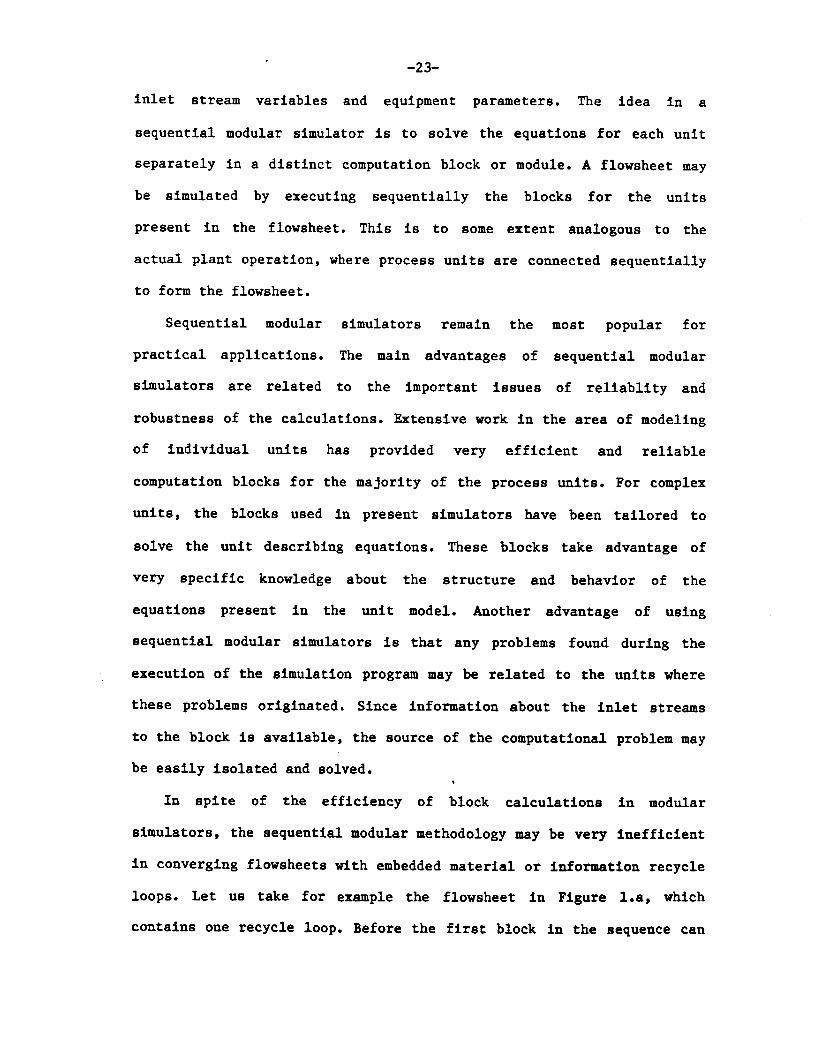
1.2.2 Sequential Modular Simulators.
Each unit in the process may be modelled by a set of unit
describing equations. These equations may be solved for the internal
unit variables and the outlet stream variables given values of the
-23-
inlet stream variables and equipment parameters. The idea in a
sequential modular simulator is to solve the equations for each unit
separately in a distinct computation block or module. A flowsheet may
be simulated by executing sequentially the blocks for the units
present in the flowsheet. This is to some extent analogous to the
actual plant operation, where process units are connected sequentially
to form the flowsheet.
Sequential modular simulators remain the most popular for
practical applications. The main advantages of sequential modular
simulators are related to the important issues of reliablity and
robustness of the calculations. Extensive work in the area of modeling
of individual units has provided very efficient and reliable
computation blocks for the majority of the process units. For complex
units, the blocks used in present simulators have been tailored to
solve the unit describing equations. These blocks take advantage of
very specific knowledge about the structure and behavior of the
equations present in the unit model. Another advantage of using
sequential modular simulators is that any problems found during the
execution of the simulation program may be related to the units where
these problems originated. Since information about the inlet streams
to the block is available, the source of the computational problem may
be easily isolated and solved.
In spite of the efficiency of block calculations in modular
simulators, the sequential modular methodology may be very inefficient
in converging flowsheets with embedded material or information recycle
loops. Let us take for example the flowsheet in Figure l.a, which
contains one recycle loop. Before the first block in the sequence can

-24-
Figure 1.a: Typical Flowsheet with Recycle Loop.
ptoduct
teactot .6pepatatomixer pu
cte .6tkeamI
.6ptittet

-25-
be executed (the mixer block), the values of the recycle stream
variables must be known. The way a sequential modular simulator
handles such a problem is by guessing values of the recycle streams
and iterating on these guesses until the recycle stream variables are
converged. Each iteration on the guessed stream involves the
sequential execution of the unit operation modules up to the block
that has the torn stream as an outlet. Updated values for the stream
variables are obtained when that module is executed. Based on the
difference between the guessed values and the updated values, a new
guess for the stream variables is computed using some convergence
method. The most common numerical methods used to converge the guessed
or "Tear" streams are direct substitution and the bounded Wegstein
method (accelerated direct substitution).
When there are multiple tear streams, each tear stream is
converged separately in a convergence loop. The convergence loops for
the tear streams are nested to achieve overall flowsheet convergence.
The sequential modular convergence procedure for the flowsheet
equations (1.1-3) is represented graphically in Figure l.b. It is
important to note that the unit describing equations must be solved in
each recycle stream convergence iteration. For complex flowsheets with
multiple recycles this method of convergence may be very inefficient.
The problem is compounded by the fact that design specifications are
treated as information recycle loops in sequential modular simulators.
If a design specification is added to the example flowsheet as shown
in Figure 1.c, an initial guess for the manipulated variable is used
to execute the modules in the design specification loop. The design
specification equation is then checked for convergence. If the

TEARSTREAM
EQUATIONS
EQUATIONSFOR EACH
UNIT
ThE
r
Figure 1.b: Graphical Representation of the Sequential ModularConvergence Approach.
-26-
DESIGNSPECIFICATIONEQUATIONS
PHYSPROPEQUA
ICALERTYTIONS

-27-
p!oduct ,SPECIFICATION SAMPLED VAR]
DECISION VARIABLE
jeed VRAL o
mixeU PUMP
,teatm zepatatmA
zptitteu
IABLES
Figure 1.c: Typical Flowsheet with a Design Specification Loop.
-28-
equation is not satisfied, a new guess of the manipulated variable is
generated using a suitable numerical technique.
The most recent sequential modular simulators like ASPEN PLUS
allow the user to use more efficient numerical techniques such as
Broyden Quasi-Newton methods to achieve simultaneous convergence of
all the tear streams (including design specifications) [1, 36].
Although such techniques result in much faster flowsheet convergence,
other modular approaches such as the one described in this work have
proven much more effective and have less problems dealing with bounds
imposed on decision variables.
1.3 The Process Optimization Problem.
Process optimization involves the determination of certain process
operating conditions such that a given objective function (performance
function) is maximized or minimized subject to design and operating
constraints. Typical optimization objectives include maximization of
an economic return, maximization of a product flow rate, minimization
of energy consumed, etc.
For this problem, it may be necessary to add to the simulation
equations a series of equipment sizing and cost correlations needed to
calculate quantities used to evaluate the objective function. For
example, if the capital cost of the plant is to be minimized, cost
correlations to compute the capital cost of the units need to be
included in the problem formulation. These correlations relate the
cost of each unit to the process operating conditions, such as flow
rates, temperatures and pressures. Such cost equations and
-29-
correlations introduce new variables and equations to the original
simulation problem. For example, the cost of a compressor may be a
function of the horsepower needed to compress the gas stream. The
horsepower may be computed from the inlet and outlet stream variables,
such as flowrates and pressures. Two new equations should then be
added to the problem,
horsepower - g(flowrates, pressures)
cost of compressor - g'(horsepower)
The cost of the compressor and the horsepower should be added to the
variable list of the original simulation problem. To simplify the
nomenclature, it will be assumed the the process variable vector x
also includes result variables that may be unrelated to the original
simulation problem but which are needed to evaluate the objective
function. These variables will be determined by some performance
equations of the form:
(1.3-1) C(x, , w) - 0
These equations are added to the original simulation problem equations
(1.1-3).
In optimization problems some feed stream variables and equipment
parameters are freed in order to provide the degrees of freedom which
are necessary to optimize the objective function. These variables,
known as decision variables, are defined in a similar way to the
decision variables for design constraints. In fact, both types of

-30-
decision variables become indistiguishable in general optimization
problems.
In terms of the nomenclature defined above, the process
optimization problem may be represented mathematically as follows:
(1.3-2) Maximize F(x, , _w)
subject to: R(x,p, w) , 0
H(x, 2, w) - 0
C(x, 2 w) - 0
G(x, 2, w) > 0
In this formulation, as in the general simulation problem formulation,
the flowsheet describing equations R include all the equations (1.1-3)
minus the equations of the form (1.1-2) for all the decision variables
(including those freed to meet design constraints in addition to the
ones freed for the optimization problem). The number of degrees of
freedom (decision variables) to be determined by the optimization
procedure is the total number of variables (including internal
variables and process parameters) minus the total number of equality
constraints (number of equations R, H and C).
It should be noted that the optimization problem formulation
(1.3-2) includes inequality constraints explicitly. These constraints
may take the form of any arbitrary function; however, the most common
inequality constraints found in practical problems are bounds on the
decision variables. The optimization algorithms used for flowsheeting
problems deal automatically with inequality constraints (see Section
7.3). Bounds also appear in simulation problems with design

-31-
constraints; however, present day simulators do not usually deal
consistently with these bounds (see for example convergence section of
ASPEN PLUS User's Manual and FLOWTRAN User's Manual, Ref. 1 and 50).
1.4 Solution of Process Optimization Problems.
There are two broad classes of methods to solve process
optimization problems: Feasible path methods and infeasible path
methods. For feasible path methods, the simulation equations (equality
constraints of problem (1.3-2)) are satisfied for every intermediate
estimate of the decision variables in the path towards the optimal
solution. Thus, for feasible path methods a simulation problem needs
to be solved for every iteration of the optimization algorithm.
For infeasible path methods, the equality constraints are
satisfied only at the final optimal solution. All the variables in the
flowsheet are adjusted simultaneously in a direction that improves the
value of the objective function and comes closer to satisfying the
flowsheet describing equations. These methods solve the process
optimization problem and the simulation problem associated with it
(through the equality constraints) simultaneously.
In contrast to standard process simulation, general process
optimization techniques have not yet been developed to the point where
they may be used routinly in practical industrial-scale problems. Most
of the work performed in process optimization may still be considered
to be at the research level. The rest of this chapter is devoted to a
review of the most relevant research work carried out in this field.

-32-
1.5 Review of the Most Relevant Previous Work in Process Optimization.
There has been a very large number of papers published in the
literature related to process flowsheet optimization. Most of the work
in this subject deals with the optimization of specific plants and may
not be generalized to general flowsheeting problems. It should be
noted that some of the work dealing with general process flowsheet
optimization also lacks generality because it is confined to
unrealistically simple models for process units (linear models, for
example). Other process optimization studies are limited to particular
combinations of process units (series of distillation columns, for
example). The work reviewed in this section was selected on the basis
of its possible extension to general flowsheeting problems.
To evaluate the performance of a process optimization algorithm
three different criteria will be used:
(1) Reliability and generality of the method.
(2) Number of "Simulation Time Equivalents", defined as the ratio
of the total computer time used in the optimization to the time
needed to converge a single flowsheet simulation problem.
(3) Total number of flowsheet passes.
In this context, the term flowsheet simulation refers to the
solution of the flowsheet describing equations (without design
specifications) by converging tear stream variables in a sequential
modular simulator. An iteration within a flowsheet simulation using a
modular system is defined as a flowsheet pass.

-33-
It should be emphasized that the above criteria are independent of
the type of computer being used for the study. In terms of quantifying
the efficiency of the process optimization technique, the number of
simulation time equivalents is the most relevant measurement [8].
All the algorithms that have been developed may be classified in
five broad categories:
(1) Feasible Path Black-Box Methods.
(2) Feasible Path Sequential Modular Methods.
(3) Infeasible Path Sequential Modular Methods.
(4) Infeasible Path Equation Oriented Methods.
(5) Simultaneous Modular Methods.
Each one of these categories will be discussed separately in the
following sections.
1.5.1 Feasible Path Black-Box Methods.
These methods are characterized by their treatment of the process
as a "Black-Box", where no information about the flowsheet or the
units in the process is used to help determine the values of the
decision variables. Case study approaches to process optimization
using existing process simulators may be considered in this category.
The computational sequence in these methods is the following:
(1) Provide initial estimates of decision variables.
(2) Solve simulation equations, including design constraints
(Equations 1.1-5).

-34-
(3) Evaluate objective function and inequality constraints.
(4) Test for convergence to optimal solution. If optimal solution
has been obtained then stop.
(5) Use nonlinear programming routine to obtain a new guess of the
decision variables.
(6) Go to Step 2.
Any process simulation package, sequential modular or equation
oriented, may be used to solve the simulation problems in Step 2.
However, most of the work carried out using this approach has been
with sequential modular simulators.
The results obtained by Gaddy [5, 38] may be considered typical
for this kind of approach. Simulation time equivalents of more than
100 were observed in most problems presented in these studies, making
the methodology undesirable for the solution of large scale problems.
In addition to the large amount of computer time used during the
solution of the problem, algorithmic difficulties could be encountered
if an infeasible simulation problem was formulated for an intermediate
value of the decision variables. This problem, and the large amount of
computer time needed to compute numerically gradients of the objective
function (a simulation problem would have to be reconverged for each
numerical perturbation) have forced the use of rather inefficient
pattern search or random search methods for the optimization problem.
1.5.2 Feasible Path Sequential Modular Methods.
These methods represent an improvement over the "Black-Box"

-35-
methods described in the previous section. The idea is to use some
information about the flowsheet to generate the new estimates of the
decision variables. The first general algorithm of this type was
proposed by Hughes [25], and Parker [42] developed a specific
implementation. The computational sequence for the method developed by
Parker is as follows:
(1) Provide initial values for the decision variables.
(2) Solve the simulation equations, including design constraints.
(3) Generate an approximate set of equations to relate the outlet
stream variables to the inlet variables and equipment parameters
for each unit. This approximation is quadratic with respect to the
decision variables and linear with respect to the other stream
variables. The coefficients for the approximate equations are
computed by numerical perturbation around the computation modules
used to simulate each unit in the simulator.
(4) Generate a quadratic approximation to the objective function
taking into consideration all the cost and performance relations
which do not appear in the original simulation problem.
(5) Solve the nonlinear programming subproblem resulting from the
approximate objective function. The approximate unit equations and
the flowsheet connectivity relations were treated as equality
constraints. Obtain a new guess for the decision variables.
(6) Test convergence criterion of process optimization problem.
Stop if solution has been obtained.
(7) Go to Step 2.
Simulation time equivalents between 50 and 100 are typical for
problems solved using this algorithm.
Biegler [8] proposed two more efficient feasible path methods
-36-
designed specifically for use in sequential modular simulators. These
algorithms deal directly with the tear stream equations for the
flowsheet. For a process with recycle streams, the simulation problem
will be converged when the following tear stream equations are
satisfied:
(1.5.2-1) T(t) - t - t 0
Here the vector t represents the variables in all the tear streams in
the process. As it was mentioned in Section 1.2.2, sequential modular
simulators guess values of the tear stream variables, and iterate
around the flowsheet to update the guessed values of these variables.
Equations (1.5.2-1) simply indicate that the updated values of the
tear stream variables are the same as the values obtained in the
previous iteration. Sequential modular feasible path methods require
that these equations are converged before an optimization step is
taken.
The methods proposed by Biegler work in the following way:
(1) Provide initial values for the decision variables.
(2) Solve the simulation equations not including design
specifications. This is equivalent to satisfying the tear stream
equations (1.5.2-1).
(3) Compute the partial derivatives of the tear stream equations
(T), design specifications (H) and objective function (F) with
respect to the tear stream variables t. This operation is carried
out by perturbing numerically each tear stream variable and
performing a sequential modular pass around the loop for each
derivative in the matrix.

-37-
(4) Compute numerically the partial derivatives of the tear stream
equations (T), design specifications (H) and objective function
(F) with respect to the decision variables u.
(5a) For the first algorithm solve the optimization problem:
(1.5.2-2) Minimize F(u)
subject to H(t,u) - 0
G(t,u) 0
Since the tear stream equations are eliminated from the
optimization problem, the calculation of reduced gradients
(constrained derivatives) is required for its solution.
(5b) For the second algorithm, the following optimization problem
is solved:
(1.5.2-3) Minimize F(u)
subject to T(t,u) - 0
H(t,u) = 0
G(t,u) 0
Biegler used the Successive Quadratic Programming algorithm
developed by Wilson, Han and Powell (see Chapter 7) to solve the
optimization problems in step (5) of the algorithms. The results
presented by Biegler indicate that both methods require about 20 to 50
simulation time equivalents to find the optimal solution for a given
flowsheet. It should be noted that numerical derivatives with respect
to tear stream variables are necessary for the methods to converge.
The computation of derivatives and the flowsheet convergence

-38-
computations during each optimization step are probably the most time
consuming calculations in the algorithm.
1.5.3 Infeasible Path Sequential Modular Methods.
Many methods of this type have been proposed in the past but have
not found a successful implementation [21, 30, 55]. A successful
algorithm developed by Biegler [8] shares many characteristics with
the feasible path methods discussed in the previous section. The
method consists of the following steps:
(1) Provide initial values for the decision variables.
(2) Compute the partial derivatives of the tear stream equations
(T), design specifications (H) and objective function (F) with
respect to the tear stream variables t. This operation is carried
out by perturbing numerically each tear stream variable and
performing a sequential modular pass around the loop for each
derivative in the matrix.
(3) Compute numerically the partial derivatives of the tear stream
equations (T), design specifications (H) and objective function
(F) with respect to the decision variables u.
(4) Solve the optimization problem:
(1.5.3-1) Minimize F(u)
subject to T(t,u) w 0
H(t,u) -= 0
G(t,u) 0

-39-
Biegler also used Successive Quadratic Programming to solve this
optimization problem.
Note that this algorithm converges the tear stream equations at the
same time it finds the optimal solution to the problem.
In terms of efficiency, this method performs similarly to
Biegler's feasible path sequential modular methods presented before.
This method still requires the calculation of numerical derivatives
with respect to tear stream variables, and the time saved by not
converging the flowsheet at each optimization iteration is offset by
the extra number of iterations needed to obtain the optimal solution.
More research work is presently being conducted with the idea of
improving both feasible and infeasible path sequential modular
optimization methods [28].
1.5.4 Infeasible Path Equation Oriented Methods.
Equation oriented methods for process optimization use the same
principles as equation oriented methods in process simulation. The
optimization problem formulated in terms of all the flowsheet
variables (Equations 1.3-2) is solved directly using an advanced
nonlinear programming technique. Locke and Westerberg [33] have
already developed an equation oriented flowsheet optimizer which is
capable of finding the optimal solution to a flowsheeting problem in
less time than it takes to simulate the flowsheet with a modular
simulator. Even though this process optimization technique is
numerically very efficient, it has not found yet many industrial

-40-
applications [19] due to its limitations in handling the large poorly
behaved problems which are typical in chemical engineering
applications. Discontinuities and multiple roots in the flowsheet
describing equations pose numerical difficulties in existing
optimization algorithms. A lot more research on this subject is needed
before a general purpose equation oriented process optimizer is
developed.
1.5.5 The Simultaneous Modular Concept.
The basic idea behind simultaneous modular simulation is the use
of two types of models for each individual process unit: rigorous and
simple. A rigorous model for a particular unit consists of the
describing equations along with algorithms designed to solve them and
compute outlet stream variables. These models are equivalent to the
ones used in existing sequential modular process simulators to
simulate individual units.
In the simultaneous modular approach, the rigorous models are
evaluated at a base point, but the solutions from these models are
used only to determine parameters of the corresponding reduced models.
The equations describing all the reduced models are solved
simultaneously with the connectivity and design specification
relations. A new base point is generated and new simple model
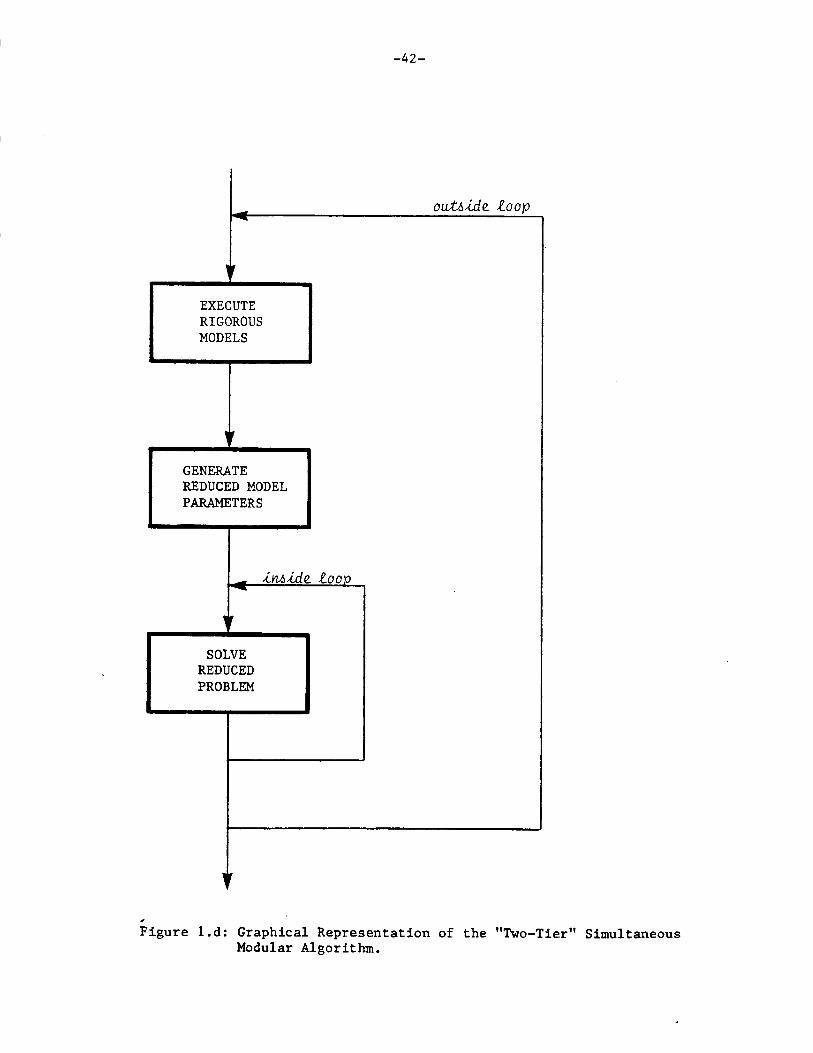
parameters are computed from the rigorous models. This "two-tier"
procedure is continued iteratively until the changes in the reduced
model parameters become sufficiently small to achieve convergence in
the process variables. The computational procedure is shown

-41-
schematically in Figure l.d. The reduced problem is in effect a system
of simulation equations analogous to the one described in Section 1.1.
However, simple models are used to model the behavior of the units and
the thermodynamic properties of the streams. The solution of the
reduced problems constitutes an "inside loop" in the overall
convergence process. The inside loop provides values of certain
variables which are used to obtain new guesses of the process
variables, so that these variables are converged in an outside loop.
Thus, this solution scheme is analogous to the "Inside-Out" algorithm
proposed by Boston for the solution of single-stage flash problems
[10] and the simulation of distillation columns [9].
It is important to notice that the system of equations resulting
from all the simple models has some desirable characteristics:
(1) It is much smaller than the system of simulation equations
that describes the flowsheet rigorously.
(2) It is much better behaved than the rigorous system.
(3) It is extremely sparse.
This allows the use of efficient equation oriented solution techniques
which would be infeasible from a practical standpoint if they were
applied to the original problem.
As it was mentioned in Chapter 1, one of the disadvantages of
sequential modular simulators is that convergence may be slow when
complex flowsheets with multiple recycles (material and design
specifications) are simulated. The reason for this is that the method
is affected by the interactions among embedded recycle calculations.
-42-
EXECUTERIGOROUSMODELS
GENERATEREDUCED MODELPARAMETERS
outside Zoop
insiLde toor)
F
Figure 1.d: Graphical Representation of the "Two-Tier" SimultaneousModular Algorithm.
SOLVEREDUCEDPROBLEM
_ I _

-43-
Equation oriented approaches, on the other hand, handle all the
recycle calculations simultaneously. The simultaneous modular approach
may be visualized as the iterative application of an equation oriented
convergence method where the reduced simulation problem is solved at
each step. The approach benefits from the desirable convergence
characteristics of efficient numerical methods; however, the
subproblems solved are much smaller and better behaved than the
original problem. At the same time, the simultaneous modular method
takes advantage of the efficient modular representations now available
for many process units.
In past studies of the simultaneous modular architecture, Pierucci
et al [44] reported an improved convergence performance over
sequential modular simulators for simulation problems with recycles.
Jirapongphan [27], and Stadtherr and Chen [53] were successful in
using this type of methodology to solve flowsheet optimization
problems using an amount of computer time comparable to that needed to
solve just the simulation problem. This suggests that general
flowsheet optimization problems could be solved is one to five
simulation time equivalents.
1.6 Objectives of this Work.
It seems feasible to develop a next generation of process
simulators/optimizers based on the simultaneous modular convergence
scheme. However, there are still some important issues that need to be
addressed before resources are spent developing a commercial

-44-
simultaneous modular simulator. The objective of this thesis is
precisely to answer the most important unresolved questions:
(1) The first issue to be considered is related to the development
of the simultaneous modular simulator itself. Jirapongphan [27]
carried out his studies using ad-hoc modifications of a simulator
already available, FLOWTRAN. His objective was to demonstrate the
feasibility of the concept; however, at the end there was no
general purpose simultaneous modular simulator that could be
expanded to solve new problems. Stadtherr and Chen [53] on the
other hand, developed a general purpose simultaneous modular
simulator from first principles. At an industrial level, this type
of development would be expensive. Since the unit operation
modules used in existing sequential modular simulators are also
needed in the new architecture, the more reasonable approach to
the problem is to take an existing simulator as starting point.
This strategy would also make it very simple for the new simulator
to initialize the calculations with sequential modular passes, as
the architecture would easily allow this type of calculations.
Furthermore, the effort to change an existing sequential modular
simulator to a simultaneous modular architecture is relatively
small compared to that needed to develop a new simulator. Chapter
3 of this thesis describes in detail how a general purpose
simultaneous modular simulator was created starting from the
existing simulator ASPEN PLUS. The main issues regarding this
conversion are treated in a general way so that the results may be
applied to other sequential modular simulators.
(2) Another issue related to the implementation of the
simultaneous modular concept is that of integration of the overall
convergence strategy with the algorithms already available in the
modules. An integrated simultaneous modular simulator could reduce
the computation time needed when the modules are executed in the
outside loop. The idea of integration is presented as part of the
general description of the algorithm in Chapter 2.

-45-
(3) The main feature of the proposed "two-tier" approach is the
use of reduced models for unit operations. The factors involved in
the development of these reduced models are discussed in Chapter
4, and some nonlinear reduced models for key unit operations are
proposed.
(4) A key aspect of this study is a comparison of the performance
of the new simultaneous modular simulator versus that of the
original sequential modular simulator. The performance of the new
simulator is affected by many parameters, such as: degree of
integration of calculations (see objective (2)); tolerances;
inside and outside-loop convergence strategies; initialization of
calculations, and heuristics used to deal with discontinuities.
The issues regarding the efficiency of calculations are discussed
in Chapter 2. Performance comparisons between the sequential
modular and the simultaneous modular versions of ASPEN PLUS are
presented in Chapter 5.
(5) The original development of the simultaneous modular concept
was based on the assumption that all the variables needed for
design specification equations are explicit in the reduced problem
[27]. A general purpose simulator must be able to handle design
specifications based on variables that would normally be avoided
in the inside loop. For example, internal variables in a staged
column and transport properties of a stream are usually not of
interest to users nor are they needed in reduced models for units.
For this reason, such variables would be excluded from the inside
loop. A general procedure is thus needed to solve problems with
design specifications, including the general case where the
variables of interest do not appear in the reduced models. This
problem is discussed in detail in Chapter 6.
(6) In realistic problems, discontinuities such as phase changes
will be present in the rigorous model equations. Methods to deal
with such discontinuities should be derived in order to have a

-46-
robust simultaneous modular simulator. Some heuristics developed
for this purpose are described in Chapter 2.
(7) The extension of the simultaneous modular approach to
optimizaton has already been tested with promising results [27,
53]. The present study focuses mainly in the use of nonlinear
reduced models for unit operations. The first issue to be
considered is the efficiency of computations as compered to the
newly developed sequential modular optimization algorithms. The
possibility of convergence to suboptimal solutions when nonlinear
models are used is studied in detail and possible solutions to
this problem are proposed. Topics related to optimization are
discussed in Chapter 7.

-47-
CHAPTER 2: SIMULTANEOUS MODULAR CONVERGENCE CONCEPT
In Chapter 1, some basic concepts of process simulation were
discussed and the most relevant work carried out in this area was
reviewed. The idea of a simultaneous modular process simulator was
introduced in Chapter 1. The present chapter is devoted to a
discussion of the main issues related to the efficiency of
simultaneous modular calculations. To simplify the discussion of the
most relevant issues, this chapter is limited to applications in
process simulation. The extension to flowsheet optimization will be
discussed in chapter 7. However, the reader should keep in mind that
the items discussed in this chapter are also relevant when the more
general optimization problem is solved.
The first section of the chapter is devoted to an explanation of
some theoretical aspects related to the use of linear and nonlinear
reduced models in simultaneous modular calculations. Section 2.2
focuses on the convergence of the outside loop. Two modes of
implementation are identified, and the advantages and disadvantages of
each one of these choices are discussed. Finally, section 2.3 is
devoted to the concept of integrated calculations in the simulator.
This is a new idea that may result in more efficient implementations
of nonlinear simultanteous modular calculations.
2.1 Linear and Nonlinear Simultaneous Modular Calculations.
Jirapongphan [27] differentiated between what he considered two

-48-
different implementations of the concept: linear simultaneous modular
and nonlinear simultaneous modular. In our view, these two approaches
differ only in the choice of reduced models used to represent the
blocks. In both cases the computational procedure is exactly the same.
However, the efficiency of the overall convergence scheme will improve
when better reduced models are used for the highly nonlinear functions
found typically in flowsheeting calculations.
Let us first look at the use of linear reduced models in detail.
In the most general form, the linear equations used to model each unit
may be expressed as:
(2.1-1) X - Ax + b
Where x and y are inlet and outlet stream variables, respectively; A
is the linear coefficient matrix and b is the residue vector. The
first "two-tier" algorithm involving linear models was developed by
Rosen [46]. In his work, Rosen used the split fraction linear models
proposed previously by Vela [58]. In the split fraction model, the
linear coefficient matrix A is diagonal with a iiy /x, and the
residue vector is zero.
Other types of linear models have been used with better
convergence results than those obtained with the split fraction model.
Naphtali [41] proposed a gradient type model. In this model each
element of the coefficient matrix, aij, is the derivative of the
ith output variable, yi, with respect to the jth input variable,
x . The elements of the coefficient matrix may be computed
numerically by finite difference as:

-49-
(2.1-2) aj j - -
ij ax x9'i j j
To carry out the finite difference approximation, each input variable
x must be perturbed to x in order to obtain the corresponding
values of the output variables y'. This requires multiple executions
of the rigorous unit model. For the units where it is satisfactory to
approximate the linear coefficient matrix with its diagonal elements
only, all the input variables may be perturbed at the same time [27].
In this case, the rigorous model only needs to be reexecuted once. It
should be noted that successive solutions of the rigorous models
during perturbation steps are not nearly as expensive to carry out as
the first solution. Since the base solution constitutes an excellent
initial guess, very few iterations are needed to converge the model
equations when only small perturbations to the input variables are
considered.
In general, the output variables from any unit operation block may
be written as a nonlinear function of the input variables,
(2.1-3) Y M f(x)
At the solution of the simulation problem, the residue function for
each block is exactly zero
(2.1-4) r(y,x) = y - f(x)
Jirapongphan shows in his thesis [27] that the use of gradient type
-50-
linear models in a simultaneous modular algorithm is equivalent to
finding the roots of the residue functions using Newton's method.
These equations would also satisfy the connectivity relations and the
design constraints imposed on the process.
Simulators that use a linear simultaneous modular approach have
been used in the past, some of them with industrial applications (see
for example reference 26). However, the equations encountered in
rigorous flowsheet calculations are usually highly nonlinear. Linear
approximations are generally poor when the solution to the reduced
problem is far from the base point where the linear coefficients are
generated. A more sophisticated approach is to use nonlinear reduced
equations based on approximate engineering models of the process
units. This will increase the range of extrapolation of the reduced
equations. However, the nonlinearity of the equations makes the
solution of the reduced problems more difficult than for the linear
case. Pierucci [44] and Jirapongphan [27] found that in spite of the
extra computations needed to solve the inside loops in the "two-tier"
algorithm, the nonlinear models increased the overall efficiency of
the method. Fewer outside loop iterations are needed to converge
(optimize in Jirapongphan's work) the flowsheet. Therefore, the number
of rigorous calculations is substantially reduced.
The present study focuses on the use of nonlinear models in the
simultaneous modular approach. A discussion of the characteristics of
reduced models is presented in Chapter 4, along with some proposed
models for complex units commonly encountered in flowsheets. In
complex optimization problems a switch from nonlinear to linear models
may be necessary to achieve convergence to the optimal solution. This

-51-
case, where linear models may play an important role in the
simultaneous modular framework, will be studied in Chapter 7.
2.2 The Outside Loop.
In the past section, the "two-tier" simultaneous modular approach
was described as an algorithm consisting of two loops that need to be
converged: An inside loop and an outside loop. The inside loop is
converged at each outside loop iteration to obtain a better
approximation to the outside loop variables. Sections 3.3.2 and 7.1,
and all of Chapter 4 are devoted to the formulation and solution of
the reduced problem in the inside loop. This section deals exclusively
with the main issues related to outside loop convergence.
2.2.1 Outside Loop Variables.
Boston and Britt [10] interpret their "Inside-out" algorithm for
single stage flash calculations as a method that uses simple model
parameters as iteration variables instead of process variables. The
advantage of this change of iteration variables is that well chosen
reduced model parameters are less dependent on process conditions than
the original process variables. For this reason, they explicitly
converge the reduced model parameters in the outside loop [3],
defining outside loop tolerances and obtaining new guesses in terms of
these parameters. Since the values of the process variables predicted
in the inside loop depend only upon the values of the reduced model

-52-
parameters, convergence of these parameters automatically assures
convergence of the original variables.
In dealing with global flowsheet convergence it is much simpler to
look at the process variables than it is to look at the model
parameters. A convergence scheme in terms of process variables is
easier to implement than a convergence scheme in terms of parameters.
Furthermore, tolerances in terms of reduced model parameters are very
difficult to define when several different unit operation blocks are
involved.
There is a choice of process variables to be converged in the
outside loop. Either all the variables present in the inside loop are
considered, or only the variables associated with feed and tear
streams along with the internal unit variables. Each one of these
choices will be discussed in detail in the next two subsections.
2.2.2 Convergence of all the Stream Variables.
The idea of keeping all the stream variables in the outside loop
is to have a set of totally independent base points to compute reduced
model parameters for the blocks. The stream and unit variables are
translated directly from the inside loop to all the streams and
variables in the flowsheet. Each rigorous computation block is then
executed independently from the others, based upon the inlet stream
values guessed from the last inside loop iteration. This may be
interpreted as a strategy where all the streams in the flowsheet are
torn and converged simultaneously in the outside loop, as shown
graphically in Figure 2.a.

-53-
---- 0o0'
mixA ectt pwnpto
Figure 2.a: Graphical Representation of a Flowsheet Converged withSimultaneous Modular Calculations, when all the StreamVariables are converged in the Outside Loop.
-54-
There are several important advantages to using this approach. The
most obvious one is that the algorithm becomes completely independent
of the structure of the flowsheet. Once the algorithm is initialized,
no information about the topology of the flowsheet (tear streams,
calculation sequence, recycle structure) is needed to continue the
calculations. Each block is independent of the rest of the process, so
that rigorous block calculations in the outside loop may be carried
out in any order.
A less obvious advantage of this outside loop formulation is
related to the concept of integrated simultaneous modular calculations
(see Section 2.3). Integrated calculations may prove important in
increasing the efficiency of the outside loop calculations by
simplifying calculations inside the rigorous computation blocks. This
approach results in unconverged solutions from the rigorous modules.
Therefore, the rigorous modules need to be executed independently to
avoid the propagation of errors from one block to another. The
discussion on integrated calculations in Section 2.3 is based on the
assumption that all the stream variables are converged in the outside
loop.
The main disadvantage of converging all the stream variables in
the outside loop is that flash calculations (enthalpy and phase
equilibrium calculations) need to be performed on every process stream
of the flowsheet every time a new outside loop iteration starts (see
Section 3.3.3). This is a lot more work than that required to reflash
only feed and tear streams, as would be the case if only these streams
were converged in the outside loop.

-55-
2.2.3 Convergence of Feed and Tear Stream Variables.
The number of variables converged in the outside loop may be
substantially reduced when only feed and tear streams are manipulated
at that level. In this approach, only the stream variables related to
feed and tear streams are translated from the inside loop to the
outside loop. Once these streams are reinitialized with updated
variables, the rigorous computation blocks are executed one after
another following a feasible calculation sequence. The new values for
all the other stream variables are computed as outputs from the
rigorous computation modules. Thus, a sequential modular pass is
executed at the beginning of each outside loop iteration, not only to
compute new simple model parameters, but also to calculate the new
guesses for the variables in streams other than the feed and tear
streams.
The above strategy may be interpreted as a very sophisticated
convergence algorithm for the tear streams in a sequential modular
simulator. The algorithm requires a tear set and a feasible
calculation sequence; thus, an analysis of the flowsheet is needed to
implement this sequential modular method. Furthermore, the choice of
tear streams may have an effect on the number of outside loop
iterations needed to converge the flowsheet.
The main advantages of this approach are related to the great
reduction in the number of manipulated variables in the outside loop.
Less streams need to be flashed during the inside-outside loop
transition (usually about ten percent of the total number of streams).
This may result in cheaper outside loop iterations, although this

-56-
advantage may be easily offset by the potential savings resulting from
integrated calculations (see Section 2.3). Another potential advantage
related to the smaller number of manipulated variables is the
possibility of using more sophisticated numerical methods to converge
the outside loop (see Section 2.2.5). For example, Broyden's
quasi-Newton method may be used to converge the outside loop. The cost
of updating the Broyden matrix during each outside loop iteration
could be too high if all the stream variables were taken into account.
However, the problem becomes more manageable when only tear and feed
streams are considered.
Comparing the two choices of outside loop variables discussed
above, our experience is that both approaches result in very similar
convergence paths. For all the example problems presented in this
thesis, the number of outside loop iterations needed to converge the
flowsheet were very similar, regardless of the choice of outside loop
variables (using direct substitution to converge the outside loop).
This result agrees with the observation reported by Kluzik [29].
2.2.4 Handling of Discontinuities.
It was mentioned in Section 2.2.1 that no sequential modular
passes on the flowsheet are needed by the simultaneous modular
algorithm if all the stream variables are considered in the outside
loop. However, sequential modular passes may be used to help
convergence even if they are not needed at each outside loop
iteration. One important use of sequential modular passes is in the
initialization of the algorithm (see Section 3.3.1). Another situation

-57-
where sequential modular passes may be used to improve the "two-tier"
algorithm is the case of discontinuities.
Let us take for example the flash drum if Figure 2.a. During
convergence of the inside loop, the vapor fraction in the flash may
reach a value of zero or one, changing the output of the flash drum
from two phases to one phase. If during the next inside loop iteration
the vapor fraction does not move again in the direction of the two
phase region, the inside loop will then converge to a solution
containing only one phase (convergence will be achieved in the next
iteration because the bounds on the value of the vapor fraction will
result in a step size equal to zero. See convergence algorithm in
Chapter 7). If this is the real solution to the problem, the algorithm
will then continue normally. However, if the real solution is not only
one phase leaving the flash, the simultaneous modular algorithm will
fail to find the real solution. The reduced equations generated after
the next outside loop update will be one phase equations, which will
not allow the possibility of having two phases in the flash drum.
One possible solution to this problem is to execute some
sequential modular passes on the flowsheet before the phase change is
accepted in the outside loop. This will drive the solution in the
right direction (either to the one phase region or to the two phase
region) before the next reduced problem is formulated. In our
implementation, two sequential modular passes are executed
automatically every time the inside loop converges because of a
discontinuity. The next outside loop iteration is then carried out
normally.
This heuristic rule used to handle discontinuities such as phase

-58-
changes is based on the built in ability of the modules in the
sequential modular simulator to deal with the problem. Equation
oriented methods cannot handle such numerical problems. For this
reason, it is the outside loop (with rigorous computation modules)
that drives the algorithm to the right region in search of the
solution. The introduction of a discontinuity in the inside loop would
create the same problems observed in equation oriented simulators
since this part of the two-tier method is solved globally.
2.2.5 Convergence of Outside Loop Variables.
The computational procedure shown in Figure l.d suggests that the
values of the variables obtained from the inside loop are used
directly as the next base point for the outside loop. This is
equivalent to using direct substitution to converge the outside loop.
Even though direct substitution is a natural choice of method, almost
any numerical procedure suitable for equation solving could also be
used. A more general computational procedure for the outside loop is
represented by the diagram in Figure 2.b. The convergence test is
applied after the inside loop is converged by comparing the previous
base point Xk with the new inside loop prediction F(Xk). If the
difference (Xk - F(Xk)) is not converged within a tolerance, a new
base point is guessed based on the previous iteration history; that is,
Xk+l - G(XkF(Xk),...)(2.2.5-1)

-59-
outs6ide loop
EXECUTERIGOROUSUNIT
MODULES
GENERATENEW GUESS OFOUTSIDE LOOPVARIABLES
GENERATEREDUCED MODELPARAMETERS
dnbzde toop
REDUCEDPROBLEM
GENERATENEW GUESS OFINSIDE LOOP
IASIABLES
CONVERGED? n
yes
CONVERGED? no
yes
Figure 2.b: General Calculation Sequence for Simultaneous ModularAlgorithm.

-60-
The method used to obtain the new base point may be simple direct
substitution:
(2.2.5-2) Xk+l w F(Xk),
Wegstein extrapolation or damping:
(2.2.5-3) Xk+l - qXk + (1-q)F(Xk)o
with q computed as a function of Xk Xk-1, F(Xk) and F(X_).
A more sophisticated convergence method would be a quasi-Newton
algorithm such as Broyden:
(2.2.5-4) Xk+l = - HF(Xk),
where H is an approximation to the inverse Jacobian of the functions
converged in the outside loop (A complete discussion of these
numerical methods may be found in the literature, see for example
reference 17).
The first two methods, direct substitution and bounded Wegstein,
were implemented in the simulator developed for this work. In general,
it was found that direct substitution was adequate for most of the
problems tested. Some form of damping (a bounded Wegstein procedure
applied to all or some subset of variables that showed oscillations
during the convergence procedure) proved very useful in reducing the
number of outside loop iterations needed to converge the flowsheet
when poor reduced models were used in the inside loop.

-61-
For the flowsheet to be converged, every single variable
manipulated in the outside loop must be converged within a given
tolerance. For this reason, it seems more appropriate to check
convergence of each outside loop variable separately, rather than
looking only at the norm of the residuals. If all the variables are to
be converged to within the same tolerance, the tolerance should be
either defined in relative terms, or applied to scaled values of the
variables. This is necessary in order to take into consideration the
large difference in magnitude between flowsheet variables.
The way the method has been defined, convergence of the outside
loop is checked before the rigorous models are executed in the outside
loop for the next iteration. It should be noted that the rigorous
models must be executed one last time after the outside loop is
converged. This procedure allows for the calculation of flowsheet
variables that do not appear in the inside loop (internal unit
variables, complex stream variables, etc.). This last execution of the
rigorous models also allows an increase in the efficiency of the
method if the last rigorous model evaluation is carried out in a
sequential modular pass.
The idea behind this last sequential modular pass is to loosen the
outside loop convergence tolerance on variables that will be computed
rigorously by the modules after convergence is achieved. Let us take
for example a flash drum where the temperature and the pressure are
specified. The heat duty will be calculated rigorously every time the
rigorous computation block is executed in the outside loop. This duty
will be exact regardless of the value computed in the inside loop,
which is the one checked for convergence purposes. Thus, as long as

-62-
the inlet stream variables are converged, the right value of the heat
duty will be computed when the rigorous model is executed. Therefore,
convergence of this variable in the outside loop is irrelevant.
Cavett's problem [14] may be used to illustrate this concept (see
flowsheet in Figure 2.c, a complete description of the problem may be
found in Section 5.3). Table 2.2-1 shows the iteration history for
simultaneous modular calculations, where only the two tear streams are
considered in the outside loop. The outside loop is converged to a
tolerance of 10-3 in the scaled variables using direct substitution,
and it takes 11 outside loop iterations (with a total of 20 inside
loop iterations) to achieve convergence. If the calculations are
analyzed in detail, we observe that after the third outside loop
iteration, the only unconverged outside loop variables are the
temperatures of the tear streams, which oscillate from one outside
loop iteration to the next. However, it is easy to see that if the
flow rates of the tear streams are converged, the correct values of
the temperatures of the tear streams will be computed if a sequential
modular pass is carried out. Thus, the outside loop iterations may be
stopped after the flowrates are converged, regardless of the error in
temperatures. Table 2.2-2 shows the iteration history for the same
problem but with the temperatures of the tear streams scaled to be two
orders of magnitude smaller than the other variables (so that the
computed variables always satisfy the outside loop tolerance). In this
case, the flowsheet is converged in 4 outside loop iterations (with a
total of 11 inside loop iterations).

-63-
dash
tear Staah
mixeA
it" h
mixeA
JZ" h
tear
Figure 2.c: Schematic Representation of Cavett's Problem showingTear Streams.

-64-
NUMBER OF ITERATIONS
Outside Loop123456789
1011
Inside Loop522222
total - 20
Table 2.2-1 .Iteration History for Cavett's Problem, Number of
Inside loop Iterations for each Outside Loop Iteration. Inside
-4 -3loop tolerance is 10 . Outside Loop Tolerance is 10 on
scaled variables. Outside loop converged using direct substitution.
NUMBER OF ITE
Outside Loop1234
RATIONS
Inside Loop5222
total - 11
Table 2.2-2 Iteration History for Cavett's problem (number of
inside loop iterations for each outside loop iteration) after
temperatures of the tear streams were eliminated from the outside-4
loop. Inside loop tolerance is 10 * Outside loop tolerance is
10-. Outside loop converged using direct substitution.

-65-
2.3 Integrated Calculations.
As it was mentioned before, the "two-tier" simultaneous modular
concept may be viewed as a generalization to the flowsheet level of
the "Inside-out" algorithm proposed by Boston [9] for equilibrium
separation devices. Inside-out algorithms also use two types of models
at two levels of convergence: simple models in an inside loop, and
rigorous models in an outside loop. When such an algorithm is used at
the module level, the knowledge of the unit operation being modelled
may be exploited to derive efficient convergence procedures for each
loop, specific to the unit. At the flowsheet level, however, two-tier
algorithms need to be very flexible in order to accomodate different
flowsheet configurations.
For a flowsheet containing unit operations modelled by inside-out
methods, a simultaneous modular simulator would include a two-tier
algorithm at the flowsheet level, and other more specialized two-tier
algorithms to converge the modules. Thus, it is possible to talk about
inside loops with simple models, and outside loops with rigorous
models within the outside loop iterations used for global convergence.
This computational scheme is represented in Figure 2.d.
A logical step would be to integrate the inside-out algorithms in
the modules with the global simultaneous modular architecture of the
simulator. Two degrees of integration are considered in this study:
(1) An Integrated Simultaneous Modular Simulator: where one or two
iterations are carried out at the module level outside loops.
Reduced model parameters are then calculated from the unconverged
solution in the block.

-66-
(2) A Completely Inside-Out Simulator: where rigorous block
calculations are reduced to the first parameter generation step in
the local inside-out algorithm. The inside loops in the blocks are
never converged. Thus, the rigorous computation blocks become just
simple model parameter generators for the global inside loop. The
computational scheme for this type of architecture is shown in
Figure 2.e.
Both implementations require that the reduced models for the units at
the flowsheet level be the simple models used in the two-tier
algorithms at the unit level.
The "Integrated Simultaneous Modular" approach may be viewed as a
modification of the standard simultaneous modular concept where
certain rigorous block calculations in the outside loop have a very
loose tolerance. The "Completely Inside-Out" concept, however, is a
new idea in process simulation. Here, the modules and the flowsheet
are converged simultaneously, saving a large number of potentially
expensive rigorous block computations.
The main advantages of integrated calculations are:
(1) Rigorous block calculations are not needed in the outside loop.
(2) The reduced models already developed for inside-out algorithms
to simulate complex separation units are also exploited at the
flowsheet level. (Models for such units as complex distillation
columns, extractors, three phase distillation, etc.). These
reduced models are usually efficient and very well suited for the
unit.
(3) The reduced model parameters generated automatically by the
modules for internal calculations are also used at the flowsheet
level.

-67-
(4) The reduced models are already implemented in the existing
modules. Some of the original code may be used directly for
reduced model formulation at the flowsheet level.
One possible disadvantage of integrated calculations is that more
outside loop iterations may be needed to converge the flowsheet,
compared to the standard implementation of the approach. However, this
problem was not observed in the example problems solved in this work,
suggesting that integrated calculations may be far more efficient than
standard two-tier algorithms. A set of example problems solved with
standard and integrated calculations is presented in Chapter 5, where
the different implementations of the simultaneous modular concept are
compared with sequential modular calculations.

-68-
EXECUTERIGOROUSUNIT
Aigowouz modeLs MODULES
paumdee
GENERATEEDUCED MODELPARAMETERS
SOLVEREDUCED
PROBLEM
Figure 2.d: Simultaneous Modular Calculations with Rigorous Modelswhich are Converged with Inside-Out Algorithms
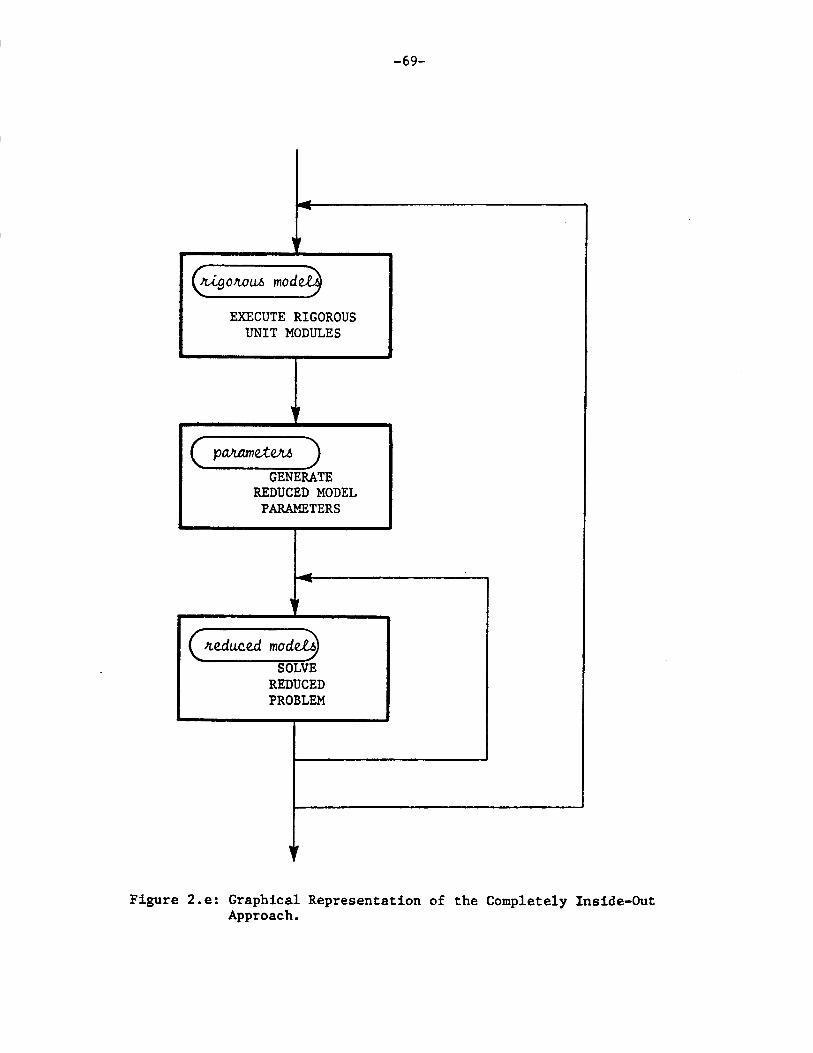
-69-
>tio~tusmod
EXECUTE RIGOROUSUNIT MODULES
patameteusGENERATE
REDUCED MODELPARAMETERS
Figure 2.e: Graphical Representation of the Completely Inside-OutApproach.
Qteduced modeSOLVE
REDUCEDPROBLEM

-70-
CHAPTER 3: DEVELOPMENT OF A SIMULTANEOUS MODULAR SIMULATOR.
The feasibility of the "two-tier" simultaneous modular concept in
process simulation and optimization has already been demonstrated in
past studies (see Chapter 2). One common weakness in past studies is
the lack of capabilities of the simultaneous modular simulator
developed to test the method. Jirapongphan [27] used ad-hoc
modifications of the FLOWTRAN simulator to run his sample problems.
The sequence of computations were controlled by means of two FLOWTRAN
control blocks (equivalent to design specification blocks in other
simulators). FLOWTRAN cost blocks were used to interface the unit
operation modules, the reduced model parameter generators and the
matrix generators with the rest of the simulator. For any given run in
this simulator the user had to specify all the new blocks in the input
file, and then use FORTRAN statements mixed among the FLOWTRAN input
lines to direct the calculations. As a result of these preparations,
each run had to be tailored differently, making it very difficult to
solve any given problem. Furthermore, the user defined computational
procedures depended upon the types of reduced models used, linear or
nonlinear. Thus, comparative problem solving was even more difficult
to perform.
If Jirapongphan's ad-hoc runs represent one extreme in the
development of a simultaneous modular simulator, the other extreme
would be to develop an entirely new simulator designed specifically to
perform computations with the proposed architecture. This the the

-71-
approach used by Stadtherr and Chen [53], and by Gorczynski et al
[26]. The advantages of designing a new simulator are clear: ease of
use; efficient calculations; potential reductions in overhead, and an
open ended general purpose simulator (once the simulator is
functional). However, the effort required to develop a new simulator
is probably too great to make this idea attractive for anything more
than a research oriented package.
The approach chosen in this study is the middle point between the
two extremes mentioned above. The idea is to take an existing general
purpose sequential modular simulator, design and implement an open
ended general purpose simultaneous modular simulator. This should be
accomplished with a minimum of modifications to the original software.
If this approach proves to be feasible, it would then be possible to
achieve significant improvements in the performance of existing
simulators at a relatively low cost.
The rest of this chapter is thus devoted to a description of the
architecture of sequential modular simulators and the changes needed
to allow them to perform simultaneous modular calculations. The
specific work performed on the ASPEN PLUS process simulator will be
discussed as an example.
3.1 Architecture of Sequential Modular Simulators.
The main idea behind sequential modular simulators is the use of
separate building-block subroutines or modules to simulate individual
process units. Each module is capable of computing the outlet stream
variables from the particular unit given values of the inlet stream

-72-
variables and the necessary equipment parameters. Once the outlet
streams are known, they may serve as inlet streams to the following
modules. The modules are then executed sequentially one after another.
For acyclic flowsheets, the simulation problem is solved when each
module is executed once. However, flowsheets usually contain recycle
loops; that is, cycles for which too few stream variables are known to
allow the equations for each unit to be solved independently. To solve
a recycle problem with a sequential modular approach, the system must
be made acyclic by "tearing" streams in the recycle loops. A tear
stream is a stream for which stream variable values are guessed
initially. Based upon the tear stream guesses, information is passed
from module to module until new values of the tear stream variables
are computed. Numerical algorithms such as direct substitution,
bounded Wegstein or Broyden quasi-Newton [59] are then used to
generate new guesses for the tear streams. This procedure is repeated
until the tear stream variables are converged within a given tolerance.
In older simulators the user was usually responsible for choosing
appropriate tear streams, generating a feasible sequence of
calculations for the modules in the flowsheet, and defining special
blocks to converge the tear streams. This situation, however, has
changed during recent years. Present day commercial simulators like
PROCESS [12] and ASPEN PLUS [1] are capable of performing an analysis
of the flowsheet structure. Stream tearing and calculation sequencing
are carried out automatically, so that for most problems, convergence
of the flowsheet is now transparent to the user. We would like to
achieve the same degree of user friendliness with the new simulator.
Even though simultaneous modular simulators use a totally

-73-
different concept to converge a flowsheet with recycles, it may still
be useful to exploit the results of the sequential modular flowsheet
analysis in the new architecture. This point will be discussed in
detail in section 3.3 of this chapter.
3.2 Calculation Control Program and Unit Operation Modules.
Regardless of the complexity of the executive system of the
package, the core of a sequential modular simulator is a calculation
control program. This program decides which module or convergence
routine should be called next, and then executes the appropriate
subroutine calls. In the simplest case, the user may have to prepare
the main control program that performs these functions, as is done in
some classroom simulators [18]. In commercial simulators, the control
program is either generated by the simulator itself tailored to the
problem at hand, or is already available in a form that may be used to
solve any problem. In every case, it is the calculation control
program that determines the architecture of the simulator.
The reason for Jirapongphan's awkward implementation of the
simultaneous modular architecture in FLOWTRAN is that he did not
modify the control program directly. Instead, control of calculations
was performed by a system of subroutines (blocks) outside the main
control program. For the implementation in this work, it was decided
to let the main control program guide the simultaneous modular
calculations directly. To accomplish this objective, the tasks
assigned to the control program had to be changed.

-74-
In a sequential modular simulator the control program executes
three main functions:
(1) Initialize inlet and tear streams.
(2) Decide which module needs to be executed next. This is done
based on the given calculation sequence and the degree of nesting
of the loops to be converged.
(3) Check for convergence of each loop (i.e status of the
convergence blocks).
The new functions assigned to the control program would be as follows:
(1) Initialize inlet and tear streams.
(2) Initialize calculations by carrying out sequential modular
passes.
(3) Direct the rigorous computation blocks to generate reduced
model parameters for the inside loop.
(4) Control the generation of information needed to converge the
inside loop (Jacobian of reduced equations, gradient of objective
function, residuals, etc.).
(5) Control solution of the reduced problem in the inside loop.
(6) Check convergence of the outside loop. If this loop is
unconverged, then the variables must be translated from the inside
loop to the outside loop.
(7) Repeat steps (3), (4), (5) and (6) until the outside loop is
converged.
When the lists of old tasks and new tasks assigned to the main
control program are compared, it seems that very extensive
modifications to the original code would be needed to accomplish the
-75-
conversion. However, this is not really true. Most of the steps
described above are almost equivalent because they employ the same
calculation control.
In the new simulator the modules are required to perform other
functions in addition to the solution of output variables given
inputs. These added functions are:
(1) Reduced model parameter generation from base case solution.
(2) Generation of the Jacobian matrix of the reduced equations.
(3) Evaluation of the residuals of the reduced equations.
These functions may have to be performed separately or in combination,
depending upon the stage of solution of the problem. As a module is
executed by the main control program, a flag may be passed to indicate
which of the above functions needs to be executed during the pass.
In sequential modular passes, the appropriate modules are executed
according to a preestablished calculation sequence. For the parameter
generation steps, the modules also need to be executed in the same
sequence to obtain the base solution for each unit. The generation of
parameters may be executed directly by the module after the rigorous
model is executed. Most of the information needed to converge the
inside loop (mainly matrices and vectors that need to be generated)
may be obtained from programs added to the original unit operation
modules. This way it would be possible to generate this information by
executing the modules in the same order as in sequential modular
passes.

-76-
3.3 Computational Procedure.
The main steps of the computational procedure in simultaneous
modular calculations were discussed in Section 2.1 . These steps are
closely related to the tasks assigned to the main control program. In
this section, each step of the computational procedure will be
discussed in detail.
3.3.1 Initialization and Parameter Generation.
The term initialization may be used at two levels. Any sequential
modular simulator needs to compute the thermodynamic condition of the
inlet streams, and to initialize tear streams and internal block
variables. However, initialization of the sequential modular method in
this context refers to the process of finding an initial guess for the
outside loop variables. A suitable base point needs to be computed for
each module before reduced model parameters are generated for the
inside loop. In principle any arbitrary base point for each unit could
be used to start the calculations. However, the original sequential
modular architecture of the simulator may be used to carry out a
number of sequential modular passes on the flowsheet. This procedure
leads to more reasonable base points.
The newest commercial simulators, ASPEN PLUS and PROCESS, carry
out flowsheet analysis using sophisticated tearing and sequencing
algorithms [1, 12, 40],. As a result of this analysis a good
calculation sequence is already known and may be used in the
initialization passes. The more basic initialization procedures needed

-77-
for the sequential modular passes, tear stream guesses and enthalpy
and phase equilibrium calculations for the inlet streams (inlet stream
flashes), also need to be performed by the original simulator;
therefore, they need not be changed in the new version.
There is one difference between the normal sequential modular
passes executed by the original simulator and the initialization
passes in the new simulator. This difference arises in the handling of
nested loops. In a normal sequential modular pass, loops nested inside
other loops need to be converged before the calculation sequence
continues in the outer loops. Thus, for for a calculation sequence of
the form shown in Figure 3.a, the modules would be executed in the
following order:
A (B C F, B C F, ... ) D E
For the case where only a feasible base point for the simultaneous
modular algorithm is needed, convergence of the inner loops is usually
not required. Therefore, a sequential modular initialization pass may
be simplified to the form:
A B C F D E
Rigorous sequential modular initialization passes may be executed for
cases where a good initial guess is necessary to converge the
calculations. This option would be equivalent to using the sequential
modular simulator to start convergence far from the solution, and then
switching to simultaneous modular calculations close to the solution.

-78-
tear
A B C D E
%tear
fF
Figure 3.a: Example of Flowsheet with Two Recycles.

-79-
From the point of view of execution, both types of passes use the
same tear streams and follow the same preestablished calculation
sequence. The only difference is that for the initialization passes,
the convergence blocks used to converge the different tear streams are
ignored. This is an important advantage of the new architecture, only
a feasible calculation sequence is required from the flowsheet
analysis step. Nested loops and convergence blocks are not needed at
any stage of the calculations.
The number of passes needed to initialize the calculations varies
from problem to problem, and may be considered a convergence parameter
set by the user. Stadtherr and Chen [53] report that for their
problems up to five passes are sometimes necessary to get a good
initial point. For the work done in this thesis it was found that two
initialization passes were almost always enough.
The first reduced model parameter generation step may be executed
directly during the last sequential modular initialization pass. The
modules may generate directly the reduced model parameters after the
rigorous solution is obtained for each module. For the cases where
some blocks have zero flow going through them at the time when the
reduced model parameters are generated, a small flow rate may be
arbirarily assumed in order to get values for the reduced model
parameters. For example, a flash block whose rigorous solution
indicates a vapor fraction of zero may be assumed to have a vapor
fraction of 0.05 (only when reduced model parameters are generated).
This way, the blocks that follow the vapor stream will have a small
flow going thorugh them during the parameter generation stage.

-80-
3.3.2 Reduced Problem Formulation and Solution.
The inside loop of the simultaneous modular procedure starts after
the reduced model parameters are generated. This part of the
calculations should be performed in equation oriented fashion, that
is, efficient numerical methods should be used to solve simultaneously
the reduced problem in the inside loop. The reduced problem is the
simultaneous solution of the system of reduced flowsheet equations if
simulation calculations are to be performed. Alternatively, for
optimization, the reduced problem would be a highly constrained
optimization problem, where the reduced flowsheet equations are
treated as equality constraints (see Chapter 7). In both cases, the
flowsheet describing equations generated in the inside loop take the
form of equations (1.1-5). The feed stream variables and the operating
parameters are specified by equations of the form (1.1-2). The
numerical methods used to solve the reduced problem (Newton-Raphson
for simulation and Successive Quadratic Programming for optimization)
require basically the same numerical information: the Jacobian matrix
and the residuals of the reduced flowsheet equations. Since the idea
of the method is to solve the inside loop problem globally, the
vectors and matrices that characterize the problem must include all
the equations in the flowsheet, and not just the reduced equations for
a single module.
There are three types of flowsheet describing equations in the
reduced problem: the equations that model the unit operations, the
connectivity relations and the design specification equations. The
information related to the equations that describe the units may be

-81-
generated by calling the modules in the same sequence as during the
initialization passes, but instructing the modules not to perform
rigorous calculations. The objective is to generate the global
information by putting together in large arrays the information from
each module. All the information needed to characterize the equations
that describe the units will be generated when all the modules have
been executed once.
There are two ways to treat the connectivity equations in a
flowsheet. The first way, used by Jirapongphan [27] , is to duplicate
each process stream in the reduced variable list. The objective is to
make the equations for a given unit basically independent of the other
units by using separate stream variables. The connectivity of the
flowsheet is then expressed in terms of network relationships, where
the outputs from certain units are equated to the inputs of other
units. This approach has the advantage of preserving a nearly block
diagonal structure of the reduced problem Jacobian matrix, as shown in
Figure 3.b. The main disadvantage of this idea is that the total
number of variables (and equations) is almost twice the number of the
real process variables because of the duplication of stream variables.
The second approach is that suggested by Stadtherr and Chen [53].
Stream variables are represented only once. The connectivity equations
are generated implicitly as the equations for a given unit are related
to the appropriate stream variables, whether these variables are
associated with a stream coming from another unit or with a stream
going to another part of the process. This approach results in a
smaller system of equations than the first approach suggested.
However, the system of equations is less structured. Thus, keeping

-82-
Figure 3.b: Structure of the Jacobian of the Reduced Problem whenStream Variables are repeated in the Problem Formulation.
unitdusenibingequations
itowsheet connectivity equationz

-83-
track of the structure during matrix generation steps is more
complicated. The work carried out by Stadtherr and Chen suggests that
the second approach results in more efficient calculations, and for
this reason it was chosen in this work (see Section 3.4.3).
The design specification equations may have any arbitrary form
given by the user. This makes their handling a particularly difficult
problem in the development of a general purpose simultaneous modular
simulator. Given the complexity of this problem, a whole chapter of
this thesis is devoted to this subject (see Chapter 6). In the
following paragraphs some general implementation aspects will be
pointed out.
In present commercial simulators the user is given much
flexibility in defining design specifications. The equations may be so
complex that any number of user defined subroutines may be needed just
to evaluate the residuals [1]. Since the form of the design
specification equations is not known a priori, the most logical way to
handle them is to have separate subroutines to evaluate the residuals.
These subroutines should be called directly by the main control
program, so that the residuals or the numerical derivatives may be
generated when needed.
There are two types of variables associated with each design
specification: the variables that appear in the equation itself, and
the variables which are "freed" to satisfy the new equation (keeping
the number of degrees of freedom). Both types of variables need to be
identified in terms of the reduced problem variables during the
initialization procedure. The information that identifies the freed
variables should be passed to the modules during the inside loop
-84-
iterations. The equations that would normally fix the values of these
variables need not be generated. For example, if a flash calculation
with temperature and pressure is specified by the user, and the
temperature is to be varied to achieve a specification, then the
equation that fixes the flash temperature to the input value should
not be generated.
The last part of the reduced problem that needs to be
characterized is the objective function to be maximized or minimized
in optimization problems. The objective function may be handled in
exactly the same way as the design specifications. The form of the
objective function is also arbitrarily defined by the user. Thus, the
simplest way to handle it is to generate a subroutine to evaluate the
value of the function, and to call this subroutine from the main
control program. The gradient of the objective function may be
generated numerically once the variables that appear in the function
are identified in terms of the inside loop variables. There are also
decision or "freed" variables associated with the optimization
problem. The information that identifies these variables also needs to
be passed to the modules in order to avoid generating the equations
that would fix their values.
In a general implementation, the simulation problem becomes just a
special case of the more general optimization problem. The algorithm
used to solve the optimization problem may also be used to solve the
system of equations found in simulation problems (see Chapter 7).
Thus, only one constrained optimization algorithm is needed to solve
any reduced problem, simulation or optimization. Similarly, the
decision variables associated with design specifications, and those

-85-
associated with the optimization problem are really indistiguishable
in the inside loop. For this reason, they are handled in the same way,
both at the problem definition and at the numerical solution levels.
There is one last important issue concerning the reduced problem:
the choice of inside loop variables. The internal block variables
associated with the unit operations will depend upon the reduced
models used to describe the units. For the nonlinear flash model used
in this study, heat duty, vapor fraction and the base equilibrium
constant are flash variables that need to be included in the inside
loop (see Section 4.3). Alternatively, a linear reduced model may only
require the heat duty as an internal variable (see section 4.2). An
important idea in the development of the inside loop is the
elimination of the internal unit variables which are not essential to
achieve convergence. As a result of this, most of the variables
present in the inside loop are stream variables.
The streams in the inside loop do not have to carry all the
information normally calculated for a stream in a simulator. A stream
may be characterized knowing only the flowrate of each component and
two variables to describe its thermodynamic condition. All the stream
information needed for the reduced models in the units may be obtained
from these variables. There are two obvious choices of variables to
characterize the thermodynamic condition of a stream: pressure and
temperature, and pressure and enthalpy. The use of the first pair of
variables makes the enthalpy balance equations for the units
nonlinear, as enthalpy equations need to be added to the reduced
models. However, all the flash calculations needed through the
computational procedure are simple pressure-temperature flashes. The

-86-
second pair of variables results in linear enthalpy balances accross
the units, but requires more complex pressure-duty flashes for other
calculations. We feel that both choices of variables are possible in a
practical implementation of the algorithm (see next section).
3.3.3 The Outside Loop Iterations.
Once the inside loop is converged, new values of the process
variables will be available. Convergence of the outside loop must be
checked at this point. One way to check convergence is to calculate
the difference between the computed inside loop variables during two
consecutive outside loop iterations. A tolerance may be defined in
terms of the maximum difference of the scaled variables or in terms of
the norm of the differences of all the scaled variables.
New guesses for the outside loop variables may be computed by any
suitable convergence method, such as direct substitution or bounded
Wegstein. The new values of the stream and unit variables should be
placed in the stream and equipment parameter vectors originally
available in the sequential modular simulator. The process streams
then need to be reinitialized in order to find all the information
required for the rigorous calculations. Finally, a new rigorous base
solution is computed by executing each module again. From this
solution, new reduced model parameters may be computed to start the
next inside loop iteration.
The transition from the inside loop to the outside loop is carried
out by placing the updated inside loop variables in the appropiate
locations of the original sequential modular simulator. Since the

-87-
stream vectors used in rigorous calculations carry more variables than
those in the inside loop, the process streams need to be
reinitialized. Depending upon the particular implementation of the
method, either all the streams of the process or only inlet and tear
streams will be flashed (see Section 2.2). And the type of flash
calculations required to reinitialize the streams will depend upon the
variables carried in the inside loop (see section 3.3.2). For this
work, the user is given the choice between converging all the streams
or only tear streams in the outside loop. The second option is
preferred for nonintegrated calculations (see Section 2.3), and
therefore is used as default. For the streams in the inside loop,
temperature and pressure were chosen to represent thermodynamic
condition. This choice of variables allows for simpler
pressure-temperature flashes during the transition from the outside
loop to the inside loop.
3.4 ASPEN PLUS Implementation.
In order to understand the procedure needed to convert the
simulator ASPEN PLUS to a simultaneous modular architecture, it is
first necessary to explain how this simulator works.
3.4.1 Steps in an ASPEN PLUS Simulation Run.
The steps involved in an ASPEN PLUS simulation are shown in Figure
3.c. The starting point is an input file written in ASPEN PLUS input
language that describes the flowsheet to be simulated (sample input

-88-
files may be found in Chapter 5. The ASPEN PLUS input language is
described in detail in reference 1. A complete description of each
step involved in an ASPEN PLUS run may be found in the first chapter
of reference 2).
The input file is interpreted by the Input Translator, which also
generates a FORTRAN program to carry out the simulation. The program
written by the Input Translator is tailored to the problem at hand
according to the information given in the input file. The simulation
program is then compiled along with any FORTRAN subroutines provided
by the user. Once the program is compiled, an executable module is
created by the loader. Only the ASPEN PLUS subroutines needed for the
particular simulation run are loaded with the main simulation program
during this step. Finally, the simulation is performed by executing
this program and a report with the simulation results is generated.
During the whole execution process, the history of the calculations
and any diagnostics generated are placed in a "History" file to help
the user understand and debug the run.
It is easy to see from the above description that ASPEN PLUS
generates its own main control program (simulation program) for each
problem (general purpose programs may be generated once to solve
several problems [1]; however, this does not alter the general
principles discussed here). As discussed before, the main control
program determines the architecture of the simulator. We shall study
the programs generated by ASPEN PLUS in more detail.
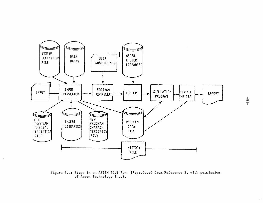
SYSTEM DATA /1 ASPENDEFINITION USER & USERFILE BANKS SUBROUTINES 9 USE
PRRAC LIBRARIES CHARAC-A
r TEPUT OTRANC FLOAERSMLTO RERTEPTFRA SLTE F MILE RP O AMW I EI
TERITIC TERSTIS HISTLRY
FILEf
Figure 3.c: Steps in an ASPEN PLUS Run (Reproduced from Reference 2, with permissionof Aspen Technology Inc.).

INSERTLIBRARIES
INSERTI NPUT PROCESSOR
SORTEDINPUTFILE
INPUTNESORT NF
INPUT FLOWSHEET PROGRAMPROCESSOR ANALYSIS 4 GENERATOR PROBLEM
DEFDNITION DATAA
F ilE BAAKA
Figure 3.d: Steps in the ASPEN PLUS Input TranslatorPermission of Aspen Technology Inc.).
(Reproduced from Reference 2, with
I

-91-
3.4.2 The Input Translator and the Structure of the Simulation Program.
In an ASPEN PLUS run, the simulation program is generated by the
input translator. The main functions of the input translator are
summarized in Figure 3.d.
The input file provided by the user is first combined with any
user defined insert files (files equivelent to subroutines written in
ASPEN PLUS input language). Since the keywords in the input file may
be in any order, the input is sorted to a preestablished order before
the input is analyzed. The input processor compares the keywords in
the input file with the accepted keywords stored in a system
definition file (a file that contains a table with all the keywords
that may be used in the simulator). The information entered using
keywords in the input file is then processed, and the information
needed from the data banks is retrieved. The next step is flowsheet
analysis. Three basic functions are carried out during this step: (1)
A set of tear streams is chosen following the criteria developed by
Upadhye and Grens [57]; (2) a feasible calculation sequence is
generated, and (3) the convergence blocks needed to converge the
material and information recycle loops are generated. The most useful
information for the new simulator is the calculation sequence.
In order to better understand how the calculation sequence is
stored and used, we should first look at the structure of the main
calling program created by the program generator. ASPEN PLUS employs
the execution monitor concept [2]. In its simplest form, the execution
monitor is a subroutine that performs some of the functions of the
main control program as discussed in Section 3.2:

-92-
(1) The monitor determines the next block to be executed.
(2) The monitor sets up block data and determines the next block
to be executed.
(3) Control is transferred to the statement that calls the block
subroutines in the main program.
(4) Upon completion of the model calculations, control is returned
to the monitor.
A simplified calling program is show below:
100 CALL MONITOR(NGOLl)GO TO (101,102), NGO
101 CALL FLASH(PLEX(Ll))GO TO 100
102 CALL SPLIT(PLEX(Ll))GO TO 100
With this scheme there is only one calling statement for each model,
regardless of the number of blocks that use the model. The block data
address, L, is different for each block. The array PLEX is a vector
that contains all the information related to the run (see a complete
description of the PLEX data structure in reference 2). The code above
could, for example, apply to a flowsheet with one FLASH block and one
SPLIT block, or to a flowsheet with 100 FLASH blocks and 50 SPLIT
blocks. Ll, which represents a pointer to the block data, has a
different value for each block. Thus, only one call for each model is
generated; a given call can be used for any number of blocks.
The actual ASPEN PLUS implementation of the monitor concept is
more complicated. Figure 3.e shows part of the main calling program
generated to simulate Cavett's [14] problem (see description of the

-93-
C *** CALL EXECUTION MONITOR TO SIMULATEREPORT, OR QUIT *80 ICALL-0
ENTRY RENTRY90 CALL EXMON (ICALL ,LPROC ,LBSMB ,LRPTWR ,SIM ,
* RPT )C DETERMINE NEXT MODEL TO CALLC AND LOCATE BLOCK BEAD AND ITS MAJOR ARRAYS100 IF (SIM)
*CALL SEQMON(IPLEX(LBSMB),IPLEX(LBSMB+11),IPLEX(LBSMB),*
*
*
NGO ,NB ,LlL4 ,L5 ,L6L9 ,L10 ,Lll
* L14 ,L15* L19 ,L20IF ( .NOT. RPT) GO TO 400
300 CALL RPTMON (IPLEX(LRPTWR),* NGO ,NB* L4 ,L5* L9 ,L10* L14 ,L15* L19 ,L20IF(IRNCLS .LT. 100) GO TO 4
500 CALL QUITGO TO 99999
400 NGO = NGO + 1GO TO (90, 101
* 102 103* ) NGO
,L16,L21
,Ll,L6,Lll,L16,L21
00
,L2,L7,L12,L17,L22
,L2,L7,L12
,L17,L22
,L3,L8,L13,L18)
,L3,L8,L13,L18
)
C101 CALL MNF001
*
*
*
*
*
GO TO 100102 CALL MNF002
*
*
*
*
*
GO TO 100103 CALL MNF003
*
*
*
*
*
GO TO 10099999 RETURN
***** CALL MODELS *****(NBIPLEX(L4)IPLEX(L8)IPLEX(L12)IPLEX(L16)IPLEX(L20)
(NBIPLEX(L4)IPLEX(L8)IPLEX(L12)IPLEX(L16)IPLEX(L20)
(NBIPLEX(L4)IPLEX(L8)IPLEX(L12)IPLEX(L16)IPLEX(L20)
,IPLEX(Ll),IPLEX(L5),IPLEX(L9),IPLEX(L13)
,IPLEX(Ll7),IPLEX(L21)
,IPLEX(Ll),IPLEX(L5),IPLEX(L9),IPLEX(L13)
,IPLEX(Ll7),IPLEX(L21)
, IPLEX(L1),IPLEX(L5),IPLEX(L9),IPLEX(L13),IPLEX(Ll7),IPLEX(L21)
,IPLEX(L2), IPLEX(L6),IPLEX(L10),IPLEX(Ll4),IPLEX(L18),IPLEX(L22)
,IPLEX(L2)
, IPLEX(L6),IPLEX(L10)
,IPLEX(Ll4),IPLEX(L18),IPLEX(L22)
,IPLEX(L2)
, IPLEX(L6),IPLEX (L10),IPLEX(L14)
,IPLEX(L18),IPLEX(L22)
,IPLEX(L3),IPLEX(L7),IPLEX(Lll),IPLEX(L15),IPLEX(L19)
,IPLEX(L3),IPLEX(L7)
,IPLEX(L1l),IPLEX(L15),IPLEX(L19)
)IPLEX(L3),IPLEX(L7),IPLEX(Lll),IPLEX(Li5)
,IPLEX(Ll9)
Figure 3.e: Sample Simulation Program Generated by ASPEN PLUS.

-94-
INITIALIZE RUN SET FLAG TO SOLVE(executed only once) =RIGOROUS MODELS
SEQlUE
no
<Z INITIALIZATIONFINISHED?
I
INTIAL
MODULAR PASS IA
yes
SET FLAG TO GENERATEPARAMETERS AND
FORMULATE REDUCEDPROBLEM
SEQUENTIALMODULAR PASS
UNSCALEVARIABLES
SET FLAG TO OBTAINNECESSARY
INFORMATION ABOUTREDUCED PROBLEM
DESIGN SPECIFICATIONS
EJECTIVE FUNCTION1
CALE VARIABLES
CALL REDUCED PROBLEM.. SOLVER
no INSIDE LOOP CONVERGED?
A
SET FLAG TO EXECUTERIGOROUS MODELS
COMPUTE PARAMETERSAND REDUCED PROBLEJ
INITIALIZE STREAMS
PLACE VARIABLESIN OUTSIDE LOOP
VECTORS ANDUNSCALE
> LOBTAIN NWGUESOUTSIDE LOOP CONVERGED? FOR SS
PROCESS VARIABLIES
yes
PLACE VARIABLESIN OUTSIDE LOOP
N SCLVECTORS ANDEUNSCALE
I
7-- =LASH STREAMS
ARESULTS PA5S I
6ENDFigure 3.f: Steps in the Simultaneous Modular Calculation Sequencing
Subroutine.
F:
II
i
00000
-95-
problem in Section 5.3). The simulation program may execute the
simulation calculations, the report writer, or both. SEQMON controls
the simulation calculations, in the same way as subroutine MONITOR in
the example shown above. RPTMON controls the report writer, and EXMON
controls whether SEQMON or RPTMON is executed. All three of these
monitors work in reverse communication mode. That is, they are called
repetitively, each time returning instructions to the main calling
program. Subroutines MNFOO1, MNF002 and MNF003 are interface routines
that call the subroutines that actually simulate the modules.
One advantage of the ASPEN PLUS architecture is that the main
calling program generated by the input translator does not have to be
directly modified to make the simultaneous modular conversion. The
control of calculations is performed by the subroutine SEQMON, which
is not altered by the input translator. Thus, if the subroutine SEQMON
is modified to perform the new functions of the main control program
described in Section 3.2, then a simultaneous modular version of ASPEN
PLUS will be available.
A flowchart describing the flow of information in subroutine
SEQMON is shown in Figure 3.f (a listing of the simultaneous modular
section of the program is included in Appendix 3). The subroutine has
all the characteristics of a simultaneous modular control program,
except that the module calls are executed by the main calling program
generated by the input translator. SEQMON decides which block should
be executed next and then passes all the information needed to execute
the module call to the main program. The type of computations to be
carried out by the modules is controlled by a flag. Other flags
control the types of reduced models to be used (linear versus

-96-
nonlinear); the stream variables converged in the outside loop (tear
and inlet streams only versus all the streams), and the convergence
method used in the outside loop (direct substitution versus bounded
Wegstein). Convergence of the inside loop is monitored directly by the
solver subroutine used to solve the reduced problem. This solver
program is written in reverse communication mode; so that it returns
repetitively to SEQMON indicating the status of the calculations and
the information needed for the next call (see description of the
algorithm in section 7.3.2. A listing of the subroutine is included in
Appendix 2).
The modules were modified as little as possible to allow for the
functions needed in the new architecture. Three sections were appended
at the end of each subroutine used to simulate a module: (1) reduced
model parameter evaluation; (2) generation of the Jacobian of the
reduced equations, and (3) evaluation of the residuals of the reduced
equations. As an example of the computer code used to perform these
functions, the simultaneous modular part of the subroutine used to
simulate a heater/pressure changer (subroutine UHE01 in ASPEN PLUS) is
included in Appendix 4. The overall information flow is a simultaneous
modular ASPEN PLUS simulation is as shown in Figure 3.g.
The reduced model parameters for each model are stored in local
retention variables which are updated once every outside loop
iteration. There are enthalpy parameters for each stream (see Chapter
4) in the process. During a parameter generation step, each module
computes the stream parameters for the outlet streams, for the inlet
tear streams, and for the inlet streams that do not come from other
blocks.

-97-
The calculation sequence generated during the flowsheet analysis
step is stored in a matrix with two columns. The first column contains
either an identification for a block to be executed, or a step number
to branch to. The second column contains the GO TO index to be used by
the main calling program in order to branch to the right subroutine
call. This information is stored sequentially in the matrix. That is,
each row in the matrix corresponds to a step to be executed. The
branches to different steps in the calculation sequence reflect the
need to loop back in order to achieve convergence in the sequential
modular simulator. Some of the blocks called in the calculation
sequence are used to handle convergence of the recycle loops. In
simultaneous modular runs, branches and convergence blocks are ignored
when a pass on the flowsheet is carried out. Therefore, the steps on
the sequence are performed straight to the end, skipping branching
steps and ignoring calls to convergence blocks.
3.4.3 Reduced Problem Formulation
In section 3.3.2, it was indicated that there are two ways to set
up the reduced flowsheet equations. The first way is to duplicate each
stream variable and then generate network type equations to model the
flowsheet connectivity explicitly. The second way is to use each
stream variable only once and keep the connectivity relations
implicit. Even though the first formulation results in a much larger
set of equations, its use may prove advantageous if very efficient
sparse matrix handling algorithms are used to decompose the Jacobian
matrix. However, in this work it was decided to follow Stadtherr's

-98-
DESIGNSPECIFICATIONS
MAINP RO GRAM S EQM ON I g 0 O B E T V
FUNCTION
REDUCEDPROBLEM
ASPEN PLUS SOLVER
INTERFACE
MODULE
INTERFACE
RIGOROUS CALCULATIONS
PARAMETER GENERATION -0OTHER SUBROUTINES
REDUCED MODELS
Figure 3.g: Information Flow in Simultaneous Modular Simulator.

-99-
VARIABLES
BLOCK 1 -
II _
Figure 3.h: Structure of the Jacobian of the Reduced Problem Generatedby the Simultaneous Modular Simulator.
STREAM 1 - - -
E
QU
A
T
I
0
N
S
BLOCK 1 - - -

-100-
suggestion and use the second formulation to reduce the size of the
problem.
In order to simplify the process of locating variables in the
reduced problem, it was decided to further sacrifice the structure of
the Jacobian matrix of the reduced simulation equations. This decision
was further justified by the fact that the programs used to factorize
the Jacobian (Harwell library subroutines MA28AD, MA28BD and MA28CD.
See documentation in reference 24) do not use algorithms that would
fully exploit a more structured matrix.
The structure of the Jacobian matrix generated by the version of
ASPEN PLUS developed in this work is shown in Figure 3.h. All the
stream variables are kept together at the beginning of the variable
list, followed by the internal variables used in each unit operation
block in the flowsheet. Each stream in the process is given a number
to identify the position of the stream vector in the variable list.
This number is chosen to match the order generated by ASPEN PLUS
during the flowsheet analysis step. Each stream vector consists of
component flowrates (ordered according to the component list used
internally by ASPEN PLUS), temperature and pressure. Thus, the size of
the stream variable section in the variable list is just the number of
components plus two times the number of streams in the flowsheet. Any
stream variable may then be located knowing the number of the stream
on the stream list and the number of components present in the
process. For example, the temperature of a given stream will be in a
position given by the following expression:
(n-1)(NC+2)+NC+l

-101-
Where n is the number of the stream and NC is the number of components.
Only a counter is needed to keep track of the equation numbers in
the reduced problem. The counter will point to the specific number of
the equation when the derivatives or the residual of the equation are
evaluated. No permanent record of the location of each equation is
needed. However, it is not difficult to identify a given equation by
looking at its position. Because of the architecture of the simulator,
all the reduced equations associated to a module will be generated
together in a preestablished order. Design specification equations are
generated at the end of the reduced problem definition step.

-102-
CHAPTER 4: REDUCED MODELS FOR UNIT OPERATIONS
The core of the two-tier simultaneous modular approach is the set
of reduced models for the unit operations, which provide the equations
for the inside loop. The first simultaneous modular algorithms used
linear models in the inside loop (see Section 2.1). However, more
recent work suggests that the use of nonlinear reduced models may
result in a significant improvement in the computational efficiency of
the overall algorithm. The purpose of this chapter is to discuss in
detail the present knowledge of reduced models. In Section 4.1 the
criteria involved in choosing adequate reduced models are discussed.
Section 4.2 is devoted to a concept in linear reduced models that uses
more information about the physical process than the models previously
used. In the remainder of the chapter new nonlinear reduced models for
some complex units commonly found in flowsheeting problems are
proposed.
4.1 Required Characteristics of Reduced Models.
The simultaneous modular concept may be viewed as a generalization
to the flowsheet level of the inside-out algorithms previously
developed to simulate individual units. Thus, the arguments
rationalized by Boston [9] in his description of individual equations
may be generalized to the reduced models for entire units. Other
criteria, such as numerical analysis -and mathematical theory, may be
used to derive other desired characteristics of reduced models. The

-103-
following is a list of the main requirements imposed on the
development of reduced models. This list represents a starting point
in the derivation of new models:
(1) The number of equations in a reduced model should be much
smaller than the number of equations solved by the rigorous unit
module.
(2) The equations in the reduced model should be well behaved.
(3) The number of degrees of freedom of a simple model should be
the same as that of the corresponding rigorous model.
(4) The variables included in a reduced model are: inlet and
outlet stream variables, equipment parameters, computed properties
and the internal variables that may be unique to the simple model.
(5) The reduced model equations should give the same solution as
the rigorous model at the base point where their coefficients are
calculated.
(6) The simple model equations and the Jacobian associated with
them should be evaluated analytically, without other auxiliary
calculations, such as thermophysical properties, and without
requiring iterative calculations.
Requirements (1) (2) and (6) guarantee that the calculations
needed to converge the inside loop are relatively simple, so that
equation oriented methods may be used to solve the reduced simulation
equations. It is desired to have a system of simulation equations that
is smaller and better behaved than the rigorous system of equations
that describe the flowsheet globally. Furthermore, the calculations in

-104-
the inside loop may be greatly simplified if the reduced equations and
their derivatives are computed analytically.
Requirement (3) insures that the problem defined in the inside
loop is equivalent to the original problem in terms of the variables
that are calculated when the simulation problem is solved. Requirement
(4) is also related to the degree of freedom analysis as it defines
the variables that must appear in the model. The choice of variables
in the model is particularly important when dealing with design
specifications, where some model parameters that are usually specified
may become variables (see Chapter 6).
Finally, requirement (5) is needed to guarantee that the
simultaneous modular procedure converges to the solution of the
rigorous simulation equations.
The list of requirements for reduced models presented above does
not impose any constraints as to the actual form of the model being
used for a unit. That is, these requirements would apply to both
linear and nonlinear reduced models. As it was mentioned before,
nonlinear models seem to be more effective in simultaneous modular
calculations. The following set of requirements was developed with the
idea of further improving the performance of nonlinear reduced models:
(7) The equations in a nonlinear reduced model should be
representative of the type of unit being modelled.
(8) The material and energy balances around each unit should
always be satisfied, even away from the base point.

-105-
(9) The expressions for the coefficients of a simple model should
be analytical. These expressions may involve any variables of the
rigorous model.
Requirements (7) and (8) indicate that the reduced models should
make use of the knowledge available of the physical process taking
place in the unit operations. The reduced models would then be
suitable engineering approximations of the rigorous equations (see for
example the reduced models presented in Section 4.3 and in Appendix
1). Such models increase the range of extrapolation of the reduced
equations away from the base points at which the model coefficients
were computed.
Requirement (9) is intended to discourage the use of gradient type
models that require the computation of numerical derivatives accross
each unit. Such calculations require a lot of computer time and should
be avoided whenever possible. Analytical expressions for the reduced
model coefficients result in increased efficiency of the parameter
generation steps in each outside loop iteration.
Requirement (5) guarantees that the solution found by the
simultaneous modular procedure for simulation problems satisfies the
rigorous simulation equations. That is, the method will converge to
the exact solution of the simulation problem. For optimization
problems, this requirement guarantees that the computed solution will
be a feasible solution to the flowsheet. However, it may be shown
through a mathematical analysis of the optimization problem (see
Section 7.2) that another requirement must be imposed on the reduced
models to guarantee convergence to the true optimal solution:

-106-
(10) The input-output Jacobian matrix predicted by a reduced model
must be the same as that predicted by the rigorous model of the
unit.
Gradient type linear models always satisfy this requirment, because
the model coefficients are the derivatives of the outlet variables
with respect to the intlet variables. The direct application of this
statement to other types of models would require the calculation of
numerical derivatives from the rigorous models in order to introduce
the appropriate correction factors in the reduced models. This
procedure, however, would introduce time consuming computations, in
direct contradiction with the statement in Requirement (9). The
proposed solution to this problem is to develop nonlinear reduced
models that have enough physical meaning to give a good approximation
to the input-output Jacobian using model parameters that may be
computed analytically. Such models might result in an suboptimal
solution which in general would be close to the real optimal solution.
If more accuarcy is required, linear models could be used in the last
outside loop iterations to reach the real optimal solution (using the
suboptimal solution obtained with the nonlinear models as a starting
point when the linear models are introduced). This procedure will be
discussed in detail in Chapter 7.
The remainder of this chapter will be devoted to a discussion of
appropriate linear and nonlinear models for flowsheet simulation and
optimization problems. It should be noted that the use of local
thermodynamic approximations of the type described by Barret and Walsh
[6] has been suggested to improve the performance of both modular and

-107-
equation oriented simulators (making the equation oriented simulator a
simultaneous modular simulator). The models used for such local
approximations fall in the same category as the reduced models
described in this chapter.
4.2 Linear Models.
Although this study is oriented towards the use of nonlinear
reduced models in simultaneous modular calculations, linear models may
be important in optimization calculations. The idea behind the use of
linear models is that the derivatives of the output variables with
respect to input variables predicted in each block by the linear model
are the same as those predicted by the rigorous models. As it was
discussed in Section 2.1, the best type of linear reduced model is a
gradient model of the form:
Where x and y are inlet and outlet stream variables, respectively; b
is the residue vector, and A is the linear coefficient matrix. Each
element of the coefficient matrix, aij is the derivative of the
ith output variable, yi, with respect to the j th input variable,
x j. The elements of this matrix need to be computed numerically by
perturbing the inlet variables to the unit and observing the
difference in the computed outlet variables.
There are two problems with this type of linear model. First, the
model does not have any physical significance. At points other than
-108-
the base case, the material and energy balances around the unit may
not be even satisfied. Furthermore, extrapolation to points far
removed from the base is usually very poor. These problems cause slow
convergence of the outside loop. The second disadvantage is the
wasteful amount of computer time needed to compute numerical
derivatives during each outside loop iteration.
The efficiency of this type of model may be increased by
substituting some of the gradient type equations by other linear
equations that do have physical significance in the unit. For example,
overall material balance equations are linear. The introduction of
these equations in the linear model will guarantee that all the
material balances around each unit are satisfied at any point. This
idea adds some engineering insight to what would otherwise be a black
box model.
Let us take as an example a two phase flash model for specified
pressure and duty (PQ Flash). The input variables are: the flow rates
for each component in the inlet stream F; the inlet stream temperature
and pressure, Tf and Pf, and the specified pressure and duty, P5
. and Q5 . The output variables are the variables associated with the
liquid and vapor outlet streams: flowrates for each component L and V,
temperatures T, and Tv, and pressures P1 and Pv The standard
gradient type linear model would take the form:
7 Ax + b

-109-
That is,
L F
p1 Pf
(4.2-1) T1 - [A] Tf + bV P- sv I .TL
For a system of n components, the matrix of coefficients A contains
(2n+4)(n+4) partial derivatives, which need to be computed
numerically. This model may be easily improved by substituting some of
the gradient type equations by rigorous linear equations. For example,
the overall component material balance equations may be included in
the reduced linear model, along with the simple relations that specify
that both outlet streams leave at the same temperature and pressure.
The following set of expressions is then obtained:
F
[Li PfLI [A'] T
s
(4.2-2) .. s
V - F-L
P - P
Pv -T - Tv 1
is simpler and more accurate than theEven though this new model

-110-
standard gradient model, the new coefficient matrix A' contains only
(n+l)(n+4) elements.
For simultaneous modular simulators that keep the stream
enthalpies in the inside loop variable list, the overall energy
balance could also be included in the linear model by adding the
following linear equation:
H - H - Hv -Q QS 0
Where H represents the total enthalpy flow of a stream.
Models such as the flash model described above were used when
linear models were needed in this study.
4.3 Nonlinear Reduced Model for Process Units.
Both Jirapongphan [27] and Pierucci [44] used nonlinear reduced
models in their work with the simultaneous modular concept. Pierucci's
nonlinear models were designed for material balance only calculations
and did not include any physical properties for energy balances or for
complex unit computations. For this reason such models can only be
used for very simple flowsheets.
Jirapongphan also developed a set of reduced models for the most
common simple units used in flowsheet simulation. He included models
for mixers, splitters, pumps, compressors, flashes and simple material
balance reactors. These models were based on reasonable engineering
approximations of the rigorous equations that describe the units, and
included terms for thermodynamic properties, such as stream enthalpies

-111-
and vapor-liquid equilibrium constants. In fact, most of the required
characteristics of simple models presented in Section 4.1 were also
rationalized by Jirapongphan when he derived the reduced models used
in his simultaneous modular simulator.
The reduced models used in this work follow the guidelines
presented at the beginning of the chapter. Some of the models for
simple units such as flow splitters, mixers, heaters, pumps,
compressors and flashes are almost equivalent to the models used by
Jirapongphan. A complete description of these models is included in
Appendix 1. An important improvement introdued in our models is the
calculation of molar stream enthalpies as enthalpy departure functions:
(4.3-1) H - HIG + A + B(T - Tref)
Where H is the molar enthalpy of the stream; HIG is the ideal gas
enthalpy of the stream; T is the stream temperature; and A, B, and
Tref are reduced model parameters obtained from the rigorously
computed stream enthalpy at a base point. The introduction of the
ideal gas enthalpy term in the enthalpy expressions introduces a
composition dependance of enthalpy in the energy balances included in
the inside loop. This type of equation was also used successfully by
Lee [32] in reduced models for distillation columns. The above
enthalpy equation is used consistently througout the flowsheet to
describe the energy balances around each unit. Since all the stream
enthalpies are computed in the same way, there is a set of enthalpy
parameters A, B and Tref for each stream in the process. All the

-112-
nonlinear reduced models include the same type of energy balance
equation.
The nonlinear reduced model for a flash unit is based on the
reduced model used in the two-tier flash algorithm available in ASPEN
PLUS (see technical documentation for this model in Reference 2). The
choice of model serves a double purpose: First, the model itself has
proven to be very effective in two-tier calculations. Second, such a
model allows for the type of integrated simultaneous modular
calculations described in Section 2.3. Since this model illustrates
all the basic principles involved in the development of nonlinear
reduced models, it will be discussed in detail in the following
paragraphs.
Let us consider a flash drum with one feed stream containing n
components, a vapor outlet stream and a liquid outlet stream. The
first set of equations that any nonlinear reduced model sould satisfy
is the material balance for each component fed to the unit. These
equations may be written in terms of component molar flows as:
(4.3-2) f - v l-i - 0
Where the variables f i V and I refer to the molar flow rates
of component i in the feed, vapor outlet and liquid outlet streams,
respectively.
The second equation that relates input and output variables is the
overall energy balance on the unit:
FHF - VHV - LHL + Q - 0(4.3-3)

-113-
Where H refers tothe molar enthalpy of stream j (j F for the
feed, V for the vapor outlet and L for the liquid outlet); F, V and L
are the total molar flow rates for the feed and outlet streams, and Q
is the heat added to the unit. In general, the enthalpy of a stream is
a function of temperature, pressure and composition. As it was
mentioned before, the molar enthalpy of each stream is calculated as
an enthalpy departure function of the form:
(4.3-4) H - HIG + A + B(T - Tref
The distribution of the components in the outlet streams is
determined by the phase equilibrium equations. For these equations,
relative volatilities were chosen as reduced model parameters due to
their small dependence on temperature, pressure and composition. For a
component i, the vapor-liquid equilibrium constant Ki may be
expressed in terms of the relative volatility by the following
equation:
(4.3-5) Ki = aiKb
Where a, is the relative volatility of component i and Kb is a
reference equilibrium constant. The value of Kb at the base point is
defined following the development by Boston and Britt [10]:
n(4.3-6) ln Kb E wi ln Ki
in

-114-
Where w are weighting factors which are defined as:
wj - t/ Et
ti - yi/(l - a - Ki)
The variable y, denotes the mole fraction of component i in the
vapor outlet stream, and 8 is the vapor fraction,
a - V/F
Once the value of Kb is determined at the base point, the values
of the relative volatilities may be computed from the rigorously
computed equilibrium constants through the following relationship:
(4.3-10) ai K /Kb
These parameters are assumed constant in the reduced model due to
their small dependance on process variables. To account for the
dependence of equilibrium constants on temperature and pressure, use
is made of the fact that these parameters are represented very well
over small ranges of these variables by a model of the form:
ln(KbP) - a + b(+ -
(4.3-7)
and
(4.3-8)
(4.3-9)
(4.3-11)

-115-
Where T* is some reference temperature, and a and b are parameters
which have a small dependence on temperature and pressure. The reduced
model coefficients in this equation are computed at the base point as
follows. From the definition of Kb in the above equation, b can be
derived as:
(4.3-12) b (ln Kb)a(1IT)
The derivative term is evaluated numerically by computing the
equilibrium constants, K ', at a perturbed temperature T', holding
the composition and pressure constant. Kb' at the perturbed
temperature is then computed using equation (4.3-6), and the
expression for b becomes:
(4.3-13) b - ln(Kg) - ln(Kb(1/T') -(l/T)
The coefficient a may be solved directly from equation (4.3-6).
The relationship between the outlet composition and the vapor-
liquid equilibrium parameters may be found through a combination of
the equilibrium and constitutive equations:
(4.3-14) vi(1 - $) - aiKblia = 0
The last equations in the model are also equilibrium equations,
which state that both outlet streams leave at the same temperature:
435TT -T - 0(4.3-15)

-116-
The reduced model includes 2n+8 equations (equations (4.3-2),
(4.3-3), (4.3-4), (4.3-6), (4.3-9), (4.3-11), (4.3-14) and (4.3-15))
with 3n+ll variables (fi, lip vi, TF, TL, TV, P, a, Q and
Kb). The reduced model parameters to be determined at the base point
are the relative volatilities, ai, the two Kb model coefficients
and the enthalpy parameters for the feed and outlet streams.
It should be emphasized that this reduced model complies with all
the requirements mentioned in Section 4.1, with the only exception of
requirement (10). As shown by Jirapongphan [27], the number of
equations is much smaller than for the rigorous flash model. The
equations are well behaved, they have physical meaning, and their
Jacobian may be evaluated analytically. Note that when all the feed
conditions are specified (f and TF), there are only two degrees
of freedom left to completely define the problem, which is the same
number of degrees of freedom found in a rigorous flash model. Thus,
the degree of freedom analysis complies with the third requirement for
reduced models.
Models for complex separation units have also been developed as
part of this effort to test the simultaneous modular concept in an
industrial simulator. Not all of these models have been adapted to the
process simulator described in this thesis. However, because of the
importance of the concepts involved in these models, the next
subsection will be used to describe these models briefly.

-117-
4.3.1 Reduced Model for Absorber Columns.
A reduced model has been developed for multistage, adiabatic
absorbers. Although this model has not yet been adapted to the
simultaneous modular simulator developed in this study, tests using a
wide variety of conditions have been conducted and published by
Trevino-Lozano, Kisala and Boston [56]. This model constitutes a good
illustration of the application of the principles described in Section
4.1 to a real complex unit. For this reason, the model will be
described in detail.
To present the reduced model, let us consider an absorber column
with N stages (see schematic on Figure 4.a). The first equation that
any mathematical model of the absorber should satisfy is an overall
material balance, which may be written in terms of component flows as:
(4.3.1-1) Uli,N+l 1 ,1 l- (vi,N - vi,O 0
The second equation that relates input and output variables is the
overall energy balance on the column:
(4.3.1-2) + +l + V0 H0 - L 1 - VN
Where H refers to the molar enthalpy flow of stream j. In general,
the enthalpy of a stream is a function of temperature, pressure and
composition.
Since the effect of temperature is typically much stronger than

-118-
VN LN+l
LOL
6tr e N
.6tatge 3
.tge 2
z6tage I
Figure 4.a: Diagram of an Absorber Column.

-119-
that of other variables, and heat capacity is a relatively weak
function of temperature, the molar enthalpy may be approximated by the
following expression:
(4.3.1-3) H = HIG + A + B(T - Tref
In order to perform an energy balance on the absorber column using
equation (4.3.1-3) to model the enthalpy of each stream, a set of
parameters "A" and "B" are calculated for each stream from the results
or the rigorous model calculations. The values are obtained from two
enthalpy values, one at Tref and the second at a perturbed
temperature, with composition held constant.
The overall material and energy balances give relationships that
the inlet and outlet streams must satisfy. However, they do not
determine the distribution of components in the outlet streams. The
distribution is determined by two additional types of equations that
are used in the reduced analytical model: phase equilibrium equations
for the top and bottom stages; and "short-cut" equations to provide an
approximate description of the multicomponent, multistage separation
behavior.
For equilibrium relationships, relative volatilities were chosen
as reduced model parameters due to their small dependence on
temperature, pressure and composition. For a component i in stage 1,
for example, the vapor-liquid equilibrium constant Ki1 may be
expressed in terms of a relative volatility by the following equation:

-120-
(4.3.1-4) K - a Kb
where a is the relative volatility of component i and Kb is a
reference equilibrium constant. Similarly, for a component in stage
N, the vapor-liquid equilibrium constant would be:
(4.3.1-5) Ki,N - aiN KbN
The reference equilibrium constants Kb and Kb are determined from the
base case rigorous model solution as a weighted average of the
component vapor-liquid equilibrium constants following the development
given by Boston and Britt [10]. For each stage:
n(4.3.1-6) ln Kb - w i ln Ki
i1m
where wi are weighting factors. In previous work with this model [56],
the vapor mole fractions yi,N are used as the weighting factors for KbNwhile for Kb , the liquid mole fractions x were used.
The error introduced by assuming that the relative volatilities of all
components in both stages stay constant when temperature, pressure, and
composition are changed from the base conditions is typically small, due
to the small dependence of relative volatilities on those variables.
However, the values of the reference equilibrium constants will depend
strongly on temperature and pressure, and to a smaller degree on
composition. To account for this dependence, equilibrium constant
equations similar to the one used in the reduced flash model are used:
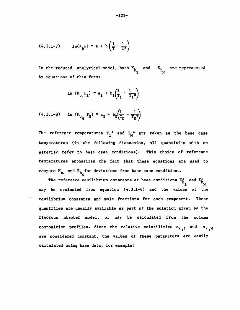
-121-
(4.3.1-7) ln(KbP) = a + b -
In the reduced analytical model, both Kb and Kb are represented
by equations of this form:
in (KP - a1 + b
(4.3.1-8) in (Kb N ) - aN + -
The reference temperatures T * and TN * are taken as the base case
temperatures (in the following discussion, all quantities with an
asterisk refer to base case conditions). This choice of reference
temperatures emphasizes the fact that these equations are used to
compute Kb1 and Kb Nfor deviations from base case conditions.
The reference equilibrium constants at base conditions and K91 N
may be evaluated from equation (4.3.1-6) and the values of the
equilibrium constants and mole fractions for each component. These
quantities are usually available as part of the solution given by the
rigorous absober model, or may be calculated from the column
composition profiles. Since the relative volatilities a 1i and ai,N
are considered constant, the values of these parameters are easily
calculated using base data; for example:

-122-
*
a K
i,N KK*'b N *N
The parameters b and bN of equation (4.3.1-8) may be obtained,
from the values of the individual K's at two temperatures, with
composition held constant.
Having defined all the simple model parameters needed to represent
the vapor-liquid equilibrium constants in the top and bottom stages of
the column, it is now possible to write an equation for each stage
that describes the physical equilibrium between the vapor and liquid
streams leaving the stage. The development of such an equation for
the top stage may be visualized as follows. Consider first the
following identity:
n n(4.3.1-10) E xi,N y iN - 1.0
where xiN and yi,N refer to the mole fraction of component i in
the liquid and vapor streams leaving stage N, respectively. Using the
criterion of vapor-liquid equilibrium the above expression becomes:
n(4.3.1-11) E y 1 N9 -- 1.0) - 0
i-1 'i,N
Finally, substituting eq. (4.3.1-5) and writing the vapor phase mole
fractions in terms of molar flows we obtain,

-123-
n 1(4.3.1-12) ivi ( i - 1.0) - 0
iN KbN
Following a similar development for the bottom stage, the following
expression may also be derived:
n(4.3.1-13) (Kb a - 1.0) 1 - 0
1
Equations (4.3.1-12) and (4.3.1-13) represent the combined phase
equilibrium and constitutive equations. Finally, in addition to the
equilibrium equations for the top and bottom stages, an approximation
to the multicomponent separation behavior in a multistage system is
needed. We have selected the Kremser equation [51], which represents
an analytical solution under certain conditions. The Kremser equation
relates the distribution of a component in the outlet streams with the
feed inputs, number of stages and average properties of the mixture in
the column. For a given component i, the Kremser equation may be
written as follows:
(,0 + li,N+l) (1.0 - S) + Li,N+l ( - S i(4.3.1-14)
- 1 (1.0 - N+l) = 0
Where Si is the average stripping factor for component i in the
column, defined as:
_ K VS - -

-124-
where Ki, V and L are the average equilibrium constant, vapor
rate and liquid rate, respectively. Clearly, the average
stripping factors will be strong functions of feed composition
and operating conditions. To introduce model parameters which
are less dependent on these variables, it is possible to follow
a parallel development as in the case of component equilibrium
constants, and define a reference stripping factor Sb, and
simple model parameters $i, which relate this reference
factor to the individual component stripping factors.
(4.3.1-15) S - i Sb
The reduced model parameters % are calculated by solving equation
(4.3.1-14) for Si for each component and calculating Sb at the
base conditions by an equation analogous to equation (4.3.1-6).
It is reasonable to assume that for deviations of the operating
conditions from the base case, the component stripping factors will
change markedly from the base values, but in such a way that the
relative changes of all components will be much smaller. This idea
may be visualized if the definition of average stripping factor is
taken into consideration. Changes in temperature and pressure, for
example, will qualitatively affect the equilibrium constants and vapor
and liquid rates in the same way, so that S would typically be
expected either to increase or to decrease for all components.
Therefore, a small dependence of $i on operating conditions may be
-125-
expected. To take into account variations of stripping factors in the
model, the reference Sb was introduced as a variable to be
determined and not as a parameter of the reduced model. This enables
the reduced model to respond properly to changes in temperature,
pressure and inlet stream conditions. Thus, in solving the reduced
model, the effective stripping factors, Si, are calculated from
equation (4.3.1-15) using a value of Sb which is determined in the
solution of the reduced model.
As mentioned above, the number of equations and degrees of freedom
are also important considerations in a reduced model. In order to
illustrate this point, degrees of freedom analyses are performed for
the reduced and rigorous models in Tables 4.3.1-1 and 4.3.1-2. The
first important thing to notice is that the reduced model is formed by
2n + 5 equations versus (3n + 3)N equations that have to be solved in
a rigorous computation. The reduction in the number of equations is
very significant, especially for big columns with a large number of
components. It is also important to point out that the number of
degrees of freedom is the same in both cases (with the only difference
being that the reduced model requires only the pressure of the top and
bottom stages, while rigorous calculations require a complete pressure
profile of the column). Therefore, outlet stream variables (flow
rates and temperatures) may be computed with both models when the
inlet stream variables, the number of stages and the pressure profile
are specified.

-126-
Table 4.3.1-1: Degree of Freedom Analysis of Reduced Analytical
Model:
1) Equations: Number
Component material balances n
Energy balance 1
Equilibrium constant models 2
Equilibrium equations 2
Constitutive equations n
2n + 5
2) Variables:
Stream component flowrates: v1 ,0; 11,1 VI,N; liN+1 4n
Stream temperatures: To, T1, TN, TN+l
Pressures: P , PN 2
Number of stages: N 1
Other: K , K , S b 3
4n + 10
Degrees of freedom: 2n + 5
Reduced model parameters that must be determined: 3n + 12
The reduced model parameters are: a ,1 aiNo $ , a 1 b1, aNbN, Al, B1 , Ao, B0, AN, BN' AN+l' BN+l

-127-
Table 4.3.1-2: Degree of Freedom Analysis of Rigorous Model of an Absorber
Column:
1) Equations:
Component material balances
Equilibrium equations
Equilibrium constant models
Energy balances
Vapor enthalpy models
Liquid enthalpy models
2) Variables:
Component liquid flowrates
Component vapor flowrates
Equilibrium constants
Inlet stream variables
Temperature at each stage
Pressure at each stage
Vapor and liquid enthalpies
Number of stages
Number
n x N
n x N
n x N
N
N
N
(3n + 3)N
n x N
n x N
n x N
2n + 2
N
N
2N
1
(3n + 4) N + 2n + 5
Degrees of freedom1 : 2n + 3 + N
(1) In the rigorous model, N degrees of freedom are used inspecifying the pressure profile. In the reduced model, only 2 areused.
-128-
4.3.2 Reduced Model for Distillation Columns.
The development of an efficient nonlinear reduced model for
distillation columns is fundamental to the practical implementation of
the simultaneous modular concept. Such a model has to be general
enough to describe complex columns: As a minimum, the model must
accomodate multiple feeds and sidestreams, internal heaters, and
non-standard configurations such as side sidestrippers. In addition,
the model should allow design specifications on internal stream
variables.
To accomplish the objectives described above, a building block
approach to model formulation was proposed. The building blocks would
be the reduced models already available for flash separators and
absorber columns. For example, a simple distillation column with one
feed, one reboiler and a condenser would consist of six blocks: The
feed plate would be described with a mixer and a flash model; the
rectifying and stripping sections would be represented by absorber
models, and two flash models would be used to describe the reboiler
and the condenser. Figure 4.b illustrates graphically the different
sections of a distillation column model. Complex columns may be easily
described by adding more sections (building blocks) to the basic
scheme. Therefore, the proposed methodology tailors the reduced model
equations according to the problem at hand avoiding unnecessary
complexity.
This idea of building the model for a given distillation column by
combining simpler units was further developed and tested by Lee [32].
His results show that the reduced models generated for a wide variety

-129-
jZazh model OVERHEAD
CONDENSER
abzoabeAmodel
RECTIFYINGSECTION
FEED Jtot6h model
FEED PLATE
absorbeAmodel
STRIPPINGSECTION
Jtah model BOTTOMS
REBOILER
Figure 4.b: Diagram of a Reduced Model for a Distillation Column.

-130-
of column configurations are very good at predicting the trends of
column performance at conditions far removed from the base point. This
was true even for moderately nonideal systems. These results suggest
that such models may be very effective for simultaneous modular
calculations in flowsheets with complex distillation columns. The only
case where this approach seemed unsatisfactory was for azeotropic
distillation. More complex reduced models are needed to represent such
highly nonideal systems.
If the flowsheet convergence algorithm is integrated with the
two-tier algoritms used in rigorous distillation modules (see Section
2.3), the type of reduced models described above could not be used. In
this case, the appropriate simple models would be the inside loop
equations of the inside-out distillation algorithms used in the
computation modules. These models are in general more complicated than
the reduced models generated from a building block approach, as
simplified tray calculations are performed at each stage (a detailed
discussion of inside-out algorithms for distillation columns may be
found in References 9 and 11). The added complexity of these models
results in better handling of highly nonideal cases such as azeotropic
distillation. For this reason, these models may also be attractive in
nonintegrated simultaneous modular calculations.
4.4 Reactor Models.
Chemical reactor modeling is still lagging in flowsheeting
applications. Most available simulators offer only simple material
balance reactors based on specified yield or specified fractional

-131-
conversion. The only industrial simulators that offer the two standard
ideal reactor models, the well stirred reactor (CSTR) and the
plug-flow reactor (PFR), are ASPEN [20] and ASPEN PLUS [1]. Even the
ideal reactor models (CSTR and PFR) are already simple models of the
complex phenomena which take place in real reactors.
The development of reduced models for chemical reactors does not
imply a refinement of the existing reactor models used in simulation.
The idea is to solve flowsheets that contain such reactor models using
simultaneous modular algorithms; therefore, a series of reduced models
with the characteristics specified in Section 4.1 need to be developed
for the reactor modules available in simulators. The rigorous reactor
models are the already idealized models such as the material balance
model, the CSTR and the PFR.
It is necessary to recognize two different types of general
reactor models for which reduced models are needed: those that contain
only algebraic equations, and those which include differential
equations. Models based on specified extents of reaction (such as XTNT
in FLOWTRAN and RSTOIC in ASPEN PLUS), models based on specified
yields (like RYIELD in ASPEN PLUS), and the commonly used CSTR model
belong to the first classification. The plug-flow reactor model is the
most important of the second class of models. The models based on
algebraic equations used currently in simulators contain material and
energy balance equations only. Reduced models for these reactors would
consist of the material balance equations (linear for the simple yield
and extent models, nonlinear for a CSTR), and an overall energy
balance equation. The reduced energy balance equation would be
analogous to the ones used in other reduced models, like equations

-132-
(4.3.1-2) and (4.3.1-3) for the absorber model. A description of some
basic reduced reactor models is included in Appendix 1).
In the case of units described by systems of differential
equations, the reduced model must represent the same unit using
algebraic equations. This is conceptually different from the problem
of finding simple algebraic equations that approximate the behavior of
other more complex algebraic equations. The solution to this problem
may be the key to expanding the simultaneous modular concept to other
problems that contain ordinary differential equations, such as dynamic
simulation and the simulation of batch plants. The next subsection
will be devoted to the description of a proposed reduced model for
plug-flow reactors. This model is general enough to be used in almost
any unit described by differential equations, including batch reactors
and rigorous continuous absorber models.
4.4.1 Reduced Model for Plug-Flow Reactors.
It is necessary to describe the plug-flow reator problem before
the reduced model is presented. Let us consider a system of n
components including reactants and all possible products. A material
stream enters the reactor at inlet temperature Ti and inlet pressure
P i(in some problems there may be multiple phases at different
temperatures flowing through the reactor. If this is the case, a
differential energy balance for each phase is necessary to compute the
different temperature profiles). The inlet flow rates of the
components in the system are represented by the vector f . A series
of reactions take place inside the reactor, and heat is added or
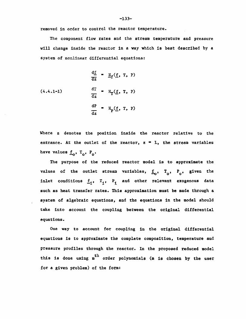
-133-
removed in order to control the reactor temperature.
The component flow rates and the stream temperature and pressure
will change inside the reactor in a way which is best described by a
system of nonlinear differential equations:
df - Hf(f, T, P)Ti-
(4.4.1-1) dT - HT(f, T, P)dz
__ M Hp~f, T, P)dz
Where z denotes the position inside the reactor relative to the
entrance. At the outlet of the reactor, z - L, the stream variables
have values f , T , P0.
The purpose of the reduced reactor model is to approximate the
values of the outlet stream variables, , T, P0, given the
inlet conditions f, Ti, P and other relevant exogenous data
such as heat transfer rates. This approximation must be made through a
system of algebraic equations, and the equations in the model should
take into account the coupling between the original differential
equations.
One way to account for coupling in the original differential
equations is to approximate the complete composition, temperature and
pressure profiles through the reactor. In the proposed reduced model
this is done using mth order polynomials (m is chosen by the user
for a given problem) of the form:

-134-
f - Aof + (Alf + ?f)z + A 2fz2 + .
(4.4.1-2) T = AOT + (AlT + 'T)z + A 2TZ + .
P - AOP + (Alp + 1 )z + A2PZ2 + .o
For the most general case, the order of the polynomials describing the
profiles of different variables may not be the same. In this case, the
number of polynomial coefficients to be determined changes; however,
the overall structure of the reduced model equations remains unchanged.
The main feature of the proposed reduced model is that the
polynomial coefficients A09 Al' A2 , etc., are not simple model
parameters. Instead, these coefficients are reduced model variables to
be determined for any given set of initial conditions. The
coefficients X are reduced model parameters which are determined from
the rigorous solution of the differential equations for the base point
initial conditions. The function of these coefficients will be
discussed later in this section.
The equations needed to determine the polynomial coefficients
A ... , are obtained from the application of collocation techniques
to linearized sets of differential equations. Given a set of m
collocation points (chosen by the user) z*, z*, ... , z, it is possible1 dem
to define a system of m(n+2) algebraic equations of the form:

-135-
n 3H k(4.4.1-3) H + r5l - (Af + A Z* + . - rr z* r r
aHk+ (Ao + ATz + .T*)
3Hkj
+ 3Hk (AOP + A1pz* +.. -P*) - Alk + 2 Az+...
For k = 1, 2, ... , n+2 (n - number of components)
j = 1, 2, ... , m (m = degree of polynomials)
The right hand side of equation (4.3.1-3) corresponds to a first order
Taylor series expansion of the derivative function H k at the
collocation point z . The value of the stream variable whose profile
is described (in differential form) by Hk is approximated by the
corresponding polynomial without the linear correction term kz.
Asterisks are used to indicate terms evaluated at the collocation
point z J
The unknowns in this system of equations are the polynomial
coefficients A1 , A2, ... , A The independent coefficients A
are determined from the inlet conditions by the following equations:
A 1f_=Of =i
A - A - T
-A OP [

-136-
The reduced model parameters to be determined from the rigorous
solution for the base inlet conditions are the elements of the
Jacobian matrix of the derivative functions H at each collocation
point. The choice of reduced model parameters may be justified by the
following arguments:
(1) The first order partial derivatives of the derivative
functions H take into account the coupling of the original system
of differential equations.
(2) The shapes of the stream variables profiles inside the reactor
(determined by the values of the partial derivatives through the
reactor) are usually less dependent on inlet conditions than the
stream variables themselves. Thus, these coefficients constitute a
better set of iteration variables for flowsheet convergence
calculations.
(3) The numerical methods used to integrate systems of ordinary
differential equations in practical engineering applications
(Gear, Episode, etc,) require the computation of derivatives at
each point along the integration [13]. Thus, the Jacobian matrix
of the differential functions at each collocation point is usually
computed automatically, so that the evaluation of the reduced
model coefficients involves no additional work.
One of the requirements of the reduced models used in simultaneous
modular calculations is that they are exact at the base point where
the parameters are computed. In the case of the plug-flow reactor
model, the collocation equations by themselves do not guarantee that
the reduced model solution matches the rigorous solution for the base

-137-
inlet conditions . In order to match the two solutions, a linear
correction function z is added to the polynomials. The correction
parameters X are computed from the difference between rigorous and
reduced solutions evaluated at the outlet of the reactor for the base
inlet conditions. Mathematically:
[Of + AfL + . .
(4.4.1-5) 1 T IAOT + AlTL + . .
P [ [;base A OP + A L +base
The correction functions are added to the collocation polynomials to
obtain the approximate stream variable profiles described by equations
(4.3.1-2).
This reactor model was successfully implemented in the sequential
modular simulator developed for this work. All the benchmark problems
in Chapters 5, 6 and 7 which involve a plug-flow reactor were solved
very efficiently using the model. As a next development in this area,
the reactor model could be adapted for flowsheets containing
continuous absorber columns or other unit operations described by
ordinary differential equations.
(1) The solutions given by the rigorous and reduced models areonly required to match at the outlet of the reactor.

-138-
CHAPTER 5: SIMULTANEOUS MODULAR SIMULATION RESULTS.
In this chapter, the results obtained from three benchmark process
simulation problems will be discussed in detail. The scope of this
chapter is limited to pure simulation problems without design
specifications, and the purpose of the study is to compare the
simultaneous modular solution methodology with the sequential modular
algorithm used originally in ASPEN PLUS. Evaluation of performance
goes beyond the direct measurement of computer time needed to solve a
given problem. Criteria such as number of flowsheet passes, number of
simulation time equivalents and reliability of the algorithm, which
were introduced in Chapter 1, will be used in the comparison of the
algorithms.
In addition to the efficiency measurements, an analysis of the
time spent in each step of the simultaneous modular algorithm is
presented. This type of analysis is necessary to predict the
performance of the simultaneous modular algorithm in problems other
than the test problems presented in this study. Furthermore, the
information obtained from this analysis may be used for future
improvements of the algorithm by properly identifying the most time
consuming steps in the calculations.
Three benchmark problems are studied in this chapter. The first
problem is a simple flowsheet with one material recycle stream.
However, this problem is difficult to solve using nonlinear
simultaneous modular calculations as it includes a plug-flow reactor
where two reactions in series are taking place. The second problem is

-139-
a process to produce cyclohexane by hydrogenation of benzene. The
flowsheet includes two recycle streams and a reactor which is modeled
with a simple mass balance reactor model. Finally, the third problem
is a version of the well known Cavett's flowsheet [14] with sixteen
components in the feed stream. These three problems are described in
detail in Section 5.1.
Section 5.2 is devoted to a description of the parameters chosen
for the simultaneous modular and the sequential modular runs
(convergence tolerances, initialization procedures, etc.). An analysis
of the performance of the standard and integrated simultaneous modular
algorithms (see Section 2.3) is presented in Section 5.3.
5.1 Benchmark Problems - Description.
Each one of the benchmark problems used in this chapter represents
a flowsheet with a special feature often encountered in simulation.
Problem 1 contains a complex unit (a plug-flow reactor) that requires
a lot of comptuer time to simulate. Problem 3 represents a flowsheet
with many material recycle loops. Problem 2, on the other hand,
represents a fairly standard flowsheet with simple units and a
straight forward topology.
5.1.1 Problem 1.
The first problem is an adaptation of a flowsheet used by Evans as
an example to demonstrate the principles of sequential modular
simulation [18]. The flowsheet is shown in Figure 5.a. This purely
-140-
hypothetical process consists of five unit operations. The feed stream
is mixed with a recycle product stream rich in unreacted raw material
in a mixer. A pump is used to increase the pressure from atmospheric
conditions to the high pressure at which the reaction takes place. The
raw material A is transformed to product P in a reactor. The product,
however, further reacts to form G, an undesirable byproduct. The
stream leaving the reactor is introduced to a flash drum to separate
the more volatile product P from the leftover A and the byproduct G.
The liquid stream leaving the flash drum is split into two fractions:
a small fraction of the stream is purged out of the process and the
rest is recycled and mixed with the feed stream.
The feed stream (stream FEED) transports 0.0126 kmol/sec of pure
reactant A at 2980K and 1 atmosphere (1.013 x 10⁵
newtons/square-meter) to the mixer. The recycle stream (stream
RECYCLE) also arrives to the mixer at atmospheric pressure. The pump
operates adiabatically to raise the pressure of the stream fed to the
6 2reactor (stream REACTIN) from 1 atmosphere to 1.0342 x 10 N/m,
The reactor may be considered to be an ideal plug-flow reactor
operating at a constant temperature of 449.820K. The length of the
reactor is 15.331 meters, and its diameter is 0.1533 meters. The rates
of the two reactions taking place in the reactor are given by
Arrhenius type kinetic expressions, which are functions of reactant
concentration and temperature:

-141-
A p P GReaction 1 Reaction 2
Reaction 1:
(5.1.1-1) - dC - (3.53 x 10⁷) exp(-35570/RT)C-=A Adt
Reaction 2:
(5.1.1-2) - dC - (53.346) exp(-23670/RT)C2P P
Where CA and CP are the concentrations of A and P respectively; T
is the temperature in degrees Kelvin, and R is the ideal gas constant
in SI units.
The flash drum is operated adiabatically at atmospehric pressure,
bringing the mixture of components leaving the reactor to the two
phase region. The vapor stream leaving the flash (stream PROD) is the
product stream rich in product P. The liquid stream (stream GUNK) is
introduced to a flow splitter. Three percent of the liquid stream is
purged (stream BLEED) and the rest (stream RECYCLE) is recycled back
to the mixer.
Following the information given in the class notes for this
hypothetical system, the physical properties were computed assuming
the following compounds in the system:
A: isobutyric acid.
P: ethyl acetate.
G: n-butyric acid
For enthalpy and equilibrium calculations, ideal properties were
assumed in the system. In terms of the ASPEN PLUS modules used to

MIXER BLOCK
mixeApump
ptug -4ow JteactoL
A -- PP - G
RECYCLE
I6ptitte
Figure 5.a: Flowsheet of Benchmark Problem 1.
FEED
PROD
REACTOUT
I - 6tas h
GUNK

-143-
;
ASPEN PLUS INPUT FILE FOR PROBLEM 1 *;IN-UNITS SIOUT-UNITS SI;
; USE IDEAL PHYSICAL PROPERTIES, OPTION SET SYSOPO;
PROPERTIES SYSOPO
; DEFINE COMPONENTS IN THE SIMULATION
COMPONENTS A ISOBUTYRIC-ACID/P ETHYL-ACETATE/G N-BUTYRIC-ACID;; * DEFINE FLOWSHEET CONNECTIVITY
;
FLOWSHEETBLOCK MIXBLOCK REACTBLOCK FLASHBLOCK SPLIT
IN-FEED RECYCLEIN-REACTININ-REACTOUTIN-GUNK
OUT-REACTINOUT=REACTOUTOUT-PROD GUNKOUT-BLEED RECYCLE
;
; * DEFINE FEED STREAM CONDITIONS
STREAM FEED TEMP=298.15 PRES=1[ATM]MOLE-FLOW A 0.0126
DEFINE OPERATING CONDITIONS OFBLOCK MIX MIXER
PARAM PRES-1.034D6BLOCK REACT RPLUG
PARAM TYPE=T-SPEC LENGTH-15.331T-SPEC 0.0 449.82STOIC 1 MIXED A -1.0/P 1.0/
2 MIXED P -1.0/G 1.0RATE-CON 1 3.525D7 3.557D4/
2 53.346 2.367D4POWLAW-EXP 1 A 1.0/
2 P 2.0BLOCK FLASH FLASH2
PARAM PRES=1[ATM] DUTY0.0BLOCK SPLIT FSPLIT
FRAC BLEED 0.03
UNIT OPERATIONS
DIAM-0.1533 PHASE-2 PDROP=0
Figure 5.b: ASPEN PLUS Input File for Benchmark Problem 1.

-144-
simulate the process, only four computation blocks were needed: The
mixer block MIXER to simulate both the mixer and the pump together;
the plug-flow reactor block RPLUG; the two outlet stream flash FLASH2,
and the flow splitter FSPLIT. The ASPEN PLUS block diagram is also
indicated in Figure 5.a, and the ASPEN PLUS input file is shown in
Figure 5.b. The report file generated by ASPEN PLUS with the complete
results for the run is included in Appendix 5. In the sequential
modular runs with ASPEN PLUS, the block HEATER was used to simulate
the mixer and the pump. The reason for this change is that the reduced
model for the mixer allows for pressure changes in the outlet stream;
therefore, the use of a heater/pressure changer module is not required.
5.1.2 Problem 2.
The second problem is a process to produce cyclohexane by
hydrogenation of benzene taken from the first chapter of the ASPEN
PLUS Introductory Manual [1]. The flowsheet is shown in Figure 5.c.
Fresh benzene (stream BZIN) and make-up hydrogen (stream H2IN) are
mixed with recycle hydrogen (stream H2RCY) and recycle benzene (stream
(CHRCY) and fed to a catalytic reactor. In the reactor, the following
reaction takes place:
C6H6 + 3H2 6H12
benzene hydrogen cyclohexane
The reactor effluent (stream RXOUT) is cooled and separated into
liquid and vapor phases in a flash drum. The liquid stream leaving the
flash drum (stream LIQ) is split and thirty percent of the original

-145-
stream is recycled (stream CHRCY) and mixed with the feed streams. The
rest of this product rich stream (stream COLFD) is taken to another
part of the plant for further processing. The vapor stream leaving the
flash (stream VAP), rich in unreacted hydrogen, is also split. Eight
percent of this stream is purged out of the process (stream PURGE) to
control the buildup of inerts in the system. The rest of the stream
(stream H2RCY) is recycled and mixed with the feed streams.
The benzene feed stream (stream BZIN) carries 0.0126 Kmol/sec of
pure benzene at 1.0342 x 10⁵ N/m2 (approximately 1 atmosphere) and
310.930K to the feed mixer. The make-up hydrogen stream (stream
H2IN) brings 0.0391 Kmol/sec of a gaseous mixture at 2.31 x 10⁶
N/m and 322.04 0K to the feed mixer. The composition of the
make-up hydrogen stream is as follows:
Hydrogen: 97.5 mole percent
Nitrogen: 0.5 mole percent
Methane: 2.0 mole percent
After the feed streams and the recylce streams are mixed in the
feed mixer, the combined stream (stream HIN) is passed through a
preheater to raise its temperature to 422.040K. The pressure at the
outlet of the preheater is 2.28 x 10⁶ N/m 2 (note that the
feed-mixer/preheatpr operation includes some pumps and compressors not
shown in the flowsheet diagram of Figure 5.c).
In the reactor, 99.8 percent of the benzene in the feed is
transformed to cyclohexane. The stream going through the reactor
undergoes a pressure drop of 1.035 x 10⁵ N/m2 and leaves the

A6pLgtteAH2RCY PURGE
VAP
H2 N HIN RXIN RXOUT ah
+H 2 0
LIQ
CHRCY COLFD
,6pt ittet
Figure 5.c: Flowsheet for Benchmark Problem 2.

-147-
ASPEN PLUS INPUT FILE FOR PROBLEM 2 *
TITLE 'HYDROGENATION OF BENZENE TO CYCLOHEXANE'IN-UNITS SIOUT-UNITS SI
; * DEFINE COMPONENTS IN THE SIMULATION;
COMPONENTS H2 HYDROGEN/N2 NITROGEN/Cl METHANE/BZ BENZENE/CH CYCLOHEXANE
; * USE REDLICH-KWONG-SOAVE EQUATION FOR PHYSICAL PROPERTIES;
PROPERTIES SYSOP3
; *DEFINE FLOWSHEET CONNECTIVITY
;
FLOWSHEETBLOCK FEED-MIX IN-H2IN BZIN H2RCY CHRCY OUT-HINBLOCK HEAT IN-HIN OUT-RXINBLOCK REACT IN=RXIN OUT=RXOUTBLOCK HP-SEP IN=RXOUT OUT=VAP LIQBLOCK V-FLOW IN-VAP OUT=PURGE H2RCYBLOCK L-FLOW IN=LIQ OUT-COLFD CHRCY
;
; *DEFINE CONDITIONS OF FEED STREAMS;
STREAM H2IN TEMP-322.04 PRES=2.31D6 MOLE-FLOW=0.0391MOLE-FRAC H2 0.975/N2 0.005/Cl 0.02
STREAM BZIN TEMP=310.93 PRES=1.034D5 MOLE-FLOW=0.0126MOLE-FRAC BZ 1
;
; DEFINE OPERATING CONDITIONS OF UNIT OPERATIONS
BLOCK FEED-MIX MIXERBLOCK HEAT HEATER
PARAM TEMP=422.04 PRES=2.275D6BLOCK REACT RSTOIC
PARAM TEMP-477.59 PRES--1.035D5STOIC 1 MIXED BZ -l/H2 -3/CH 1CONV 1 MIXED BZ 0.998
BLOCK HP-SEP FLASH2PARAM TEMP=322.04 PRES--3.45D4
BLOCK V-FLOW FSPLITFRAC PURGE 0.08
BLOCK L-FLOW FSPLITFRAC COLFD 0.7
Figure 5.d: ASPEN PLUS Input File for Benchmark Problem 1.

-148-
reactor at 477.590K. The outlet stream from the reactor (stream
RXOUT) is fed to a product cooler (a flash drum) where two phases are
formed. The cooler operates at 322.040K and has a pressure drop of
3.45 x 10⁴ N/iM2
To simulate this system, six ASPEN PLUS modules were used: A MIXER
block to simulate the feed-mixer; a HEATER block for the feed
preheater; the stoichiometric reactor model RSTOIC to simulate the
reactor; the two outlet stream flash FLASH2 for the product cooler,
and two stream splitter blocks FSPLIT to split the vapor and liquid
streams leaving the product cooler. All physical properties were
calculated based on the Redlich-Kwong-Soave Equation-of-State, which
corresponds to the physical property option set SYSOP3 in ASPEN PLUS.
The ASPEN PLUS input file for this process is shown in Figure 5.d. The
complete set of results generated by ASPEN PLUS for this flowsheet are
included in Appendix 5.
5.1.3 Problem 3.
The third problem is the separation train shown in Figure 5.e. A
feed stream Fl is mixed with the liquid leaving flash unit FLAl
(stream R1) and with the vapor leaving from the flash unit FLA3
(stream R2). This mixture (stream Zl) is fed to the second flash unit
FLA2. The vapor stream from this unit (stream Sl) is sent to the first
flash FLAl, while the liquid (stream S2) is mixed with the vapor
leaving from the fourth flash FLA4 (this is stream R3). The mixture of
these two streams (stream Z2) is fed to the third flash unit FLA3. The
liquid leaving FLA3 is sent to the fourth flash FLA4. The two products

-149-
from this separation process are the light components leaving FLAl as
a vapor stream (stream Pl), and the heavy components leaving the
fourth flash FLA4 as a liquid stream (stream P2).
The feed stream containing 16 components is introduced to the
first mixer at 310.92K and 5.617 N/m. The flow rate of each one
of the components in the feed is shown in Table 5.1.3-1. The operating
conditions for each of the four flash units in the process are as
follows:
Temperature (K) Pressure (N/Sqm)
Flash FLAl: 310.93 5.617 x 10⁶
Flash FLA2: 310.93 1.963 x 10⁶
Flash FLA3: 308.71 4.392 x 10⁵
Flash FLA4: 302.59 1.910 x 10⁵
This system was simulated in ASPEN PLUS using four flash modules
(FLASH2) and three mixer blocks (MIXER). Two different physical
property options were used in the simulation runs. One set of runs was
performed assuming ideal gas properties and Raoult's law for
vapor-liquid equilibrium calculations (this is ASPEN PLUS option set
SYSOPO). The other set of runs used the Redlich-Kwong-Soave
Equation-of-State to compute all the physical properties (option set
SYSOP3). A copy of the ASPEN PLUS input file is shown in Figure 5.f,
and a complete set of results is included in Appendix 5.

P1
Si
(FLA1)
R2
R1
F1 21 (FLA2)
R3
mixeAt(MIX1)
S2 Z2" sah
(FLA3)
(MIX2)
S3
(FLA)
P2
Figure 5.e: Flowsheet for Benchmark Problem 3.

-151-
ASPEN PLUS INPUT FILE FOR PROBLEM 3 *****
;
IN-UNIT SI;
; * DEFINE FLOWSHEET CONNECTIVITYFLOWSHEET
BLOCK MIXi IN - Fl R1 R2 OUT - Z1BLOCK MIX2 IN - S2 R3 OUT - Z2BLOCK FLA IN - S1 OUT = P1 RlBLOCK FLA2 IN w Zl OUT - Sl S2BLOCK FLA3 IN - Z2 OUT = R2 S3BLOCK FLA4 IN - S3 OUT - R3 P2
;; * DEFINE COMPONENTS AND PHYSICAL PROPERTIES
COMPONENTS N2
PROPERTIES;
C02H2SCH4C2H6C3H8C4H10-2C4H10-lC5H12-2C5H12-1C6H14-1C7H16-1C8H18-1C9H20-1C10H22-1CllH24-1SYSOP3
NITROGENCARBON-DIOXIDEHYDROGEN-SULFIDEMETHANEETHANEPROPANEC4H10-2C4H10-1C5H12-2C5H12-1C6H14-1C7H16-1C8H18-1C9H20-1C10H22-1N-UNDECANE
DEFINE FEED STREAM CONDITIONS;
STREAM F1 TEMP-310.93 PRES=5.617D6MOLE-FLOW 4.51D-4 / 0.0063 / 4.27D-4
7.61D-4 / 0.0019 / 9.96D-40.0023 / 0.0021 / 0.0010
/ 0.0038 / 0.003 / 0.0029 // 0.0014 / 0.0022 / 0.0033 // 0.0015
;
; *DEFINE OPERATING CONDITIONS OF UNIT OPERATIONS;BLOCK MIXi MIXERBLOCK MIX2 MIXERBLOCK FLAl FLASH2
PARAM TEMP-310.93 PRES-5.617D6BLOCK FLA2 FLASH2
PARAM TEMP-310.93 PRES-1.963D6BLOCK FLA3 FLASH2
PARAM TEMP=308.71 PRES=4.392D5BLOCK FLA4 FLASH2
PARAM TEMP-302.59 PRES-1.910D5
Figure 5.f ASPEN PLUS Input File for Benchmark Problem 3.

-152-
Component
Nitrogen
Carbon dioxide
Hydrogen sulfide
Methane
Ethane
Propane
Isobutane
n-Butane
2-Methyl-butane
n-Pentane
n-Hexane
n-Heptane
n-Octane
n-Nonane
n-Decane
n-Undecane
Flow Rate (Kmol/sec)
4.51 x 10⁻⁴
0.0063
4.28 x 10⁻⁴
0.0038
0.0030
0.0029
7.61 x 10⁻⁴
0.0019
9.96 x 10⁻⁴
0.0014
0.0022
0.0033
0.0023
0.0021
0.0010
0.0015
Table 5.1.3-1: Composition of Feed Stream (Stream Fl) for Problem 3.

-153-
5.2 Parameters Used in the Simulation Runs.
All the runs were made using a VAX 11/780 computer. The version of
ASPEN PLUS used both for sequential modular and for simultaneous
modular calculations corresponds to the Fall of 1984 release of the
simulator.
The following two subsections describe the specific parameters
used in the runs made to evaluate the performance of the simultaneous
modular simulator.
5.2.1 The Simultaneous Modular Runs.
In order to compare the simultaneous modular runs on a consistent
basis, adjustable parameters such as convergence tolerances and
initialization procedures need to be set consistently.
The performance of the algorithm will be judged relative to the
existing sequential modular version of ASPEN PLUS. Therefore, the
convergence criteria used in the two algorithms should be adjusted so
that both methods give answers of comparable accuracy. The sequential
modular algorithm tests convergence by comparing the updated values of
the tear stream variables with the previous values used at the
beginning of the flowsheet pass. These variables are scaled internally
by ASPEN PLUS so that the given tolerances apply to the difference
between the scaled values of the tear stream variables. Furthermore,
the convergence tolerance in ASPEN PLUS is scaled relative to the
value of the variable. The default value of the relative convergence
tolerance provided by ASPEN PLUS was used in all the sequential

-154-
modular runs. This value is set to 10-4.
As it was discussed in Section 2.2.4, the convergence criteria
used in the outside loop of the simultaneous modular calculations is a
comparison between the scaled values of the outside loop variables in
two successive iterations. Convergence is achieved when the largest
change in the values of the variables is below the given outside loop
tolerance, and this tolerance is applied on an absolute basis. This
convergence criterion is incompatible with the convergence criterion
used by ASPEN PLUS. The outside loop variables are not always the same
as the tear stream variables (see Sections 2.2.2 and 2.2.3).
Furthermore, the scaling factors used by ASPEN PLUS are not the same
as the scaling factors used in the simultaneous modular algorithm.
In order to have consistent results, several trial runs were made
with different outside loop tolerances. An outside loop tolerance was
chosen such that the sequential modular results and the simultaneous
modular results differred only in the last significant figure printed
in the report files generated by the simulator. This tolerance was a
function of the scale factors used in the run. In order to simplify
the analysis, the same scale factors were used in all the simultaneous
modular simulation runs: The molar flow rates were left unscaled, the
pressures, temperatures and enthalpies were scaled to be of the order
of unity. The outside loop tolerance used in all the simulation runs
was 10-3.
Another important choice related to the convergence of the outside
loop was discussed in Section 2.2.5. This is the relaxation of the
tolerances of the variables which are calculated automatically in the
last flowsheet pass after the outside loop is converged. The tolerance

-155-
relaxation on these variables was achieved by varying the scale
factors applied to them. The scaled variables would always have values
below the outside loop tolerance, so that the change in these
variables from one outside loop to the next would always satsify the
convegence criterion. This principle was applied to the temperatures
of streams Zl and S3 in the third benchmark problem.
The convergence criterion for the inside loop is based on the norm
of the changes in the variables during a Newton-Raphson iteration (see
Section 7.3). The choice of inside loop tolerance had an effect in the
overall efficiency of the algorithm. If the inside loop tolerance is
too tight, a lot of computer time is wasted converging the inside
loop. However, a loose inside loop tolerance may lead to convergence
problems in the outside loop. For all the simulation problems solved
in this chapter and in chapter 6, an inside loop tolerance of 104
was used with very effective results.
Finally, the last parameter affecting the efficiency of the
simultaneous modular algorithm is the number of flowsheet passes used
to initialize the method (see Section 3.3.1). For each problem there
is an optimum number of initialization passes through the flowsheet;
however, this number is not known a priori. Since the algorithm should
be able to initialize itself without the help of the user, the number
of initialization passes was fixed to two. This initialization
procedure was adequate for almost every problem. Damping in the
outside loop (see Section 2.2.5) and the automatic handling of
discontinuities (see Section 2.2.4) made the algorithm robust enough
to handle even the cases where two initialization passes were not
enough to provide a good initial estimate of the flowsheet variables.

-156-
During the execution of the simultaneous modular calculations,
many parameters used internally by the ASPEN PLUS simulator were also
used. During the first initialization pass, the tear streams were
initialized to zero, which is the ASPEN PLUS default. No initial
guesses were ever provided for any variables in the flowsheet.
Whenever a sequential modular pass was performed (for initialization
calculations, during outside loop iterations and during the reduced
problem formulation), the calculation sequence provided by the ASPEN
PLUS flowsheet analysis system was used. Furthermore, whenever an
ASPEN PLUS computation module was executed to solve the rigorous unit
models, the default convergence parameters (internal tolerances, etc.)
were always used. All the operating parameters in ASPEN PLUS are
documented in the ASPEN PLUS Introductory Manual [1] and in the ASPEN
PLUS Technical Reference Manual [3].
In every problem involving a plug-flow reactor, quadratic profiles
were used in the reduced model (see Section 4.4.1). The collocation
points chosen to generate the reduced model equations were 0.5 and
0.95 times the reactor length.
5.2.2 The Sequential Modular Runs.
All the sequential modular runs were carried out using the
defaults provided by ASPEN PLUS (as shown in the input files included
in Section 5.1). These defaults include the flowsheet analysis
performed by the simulator, the choice of tear streams, the initial
values for tear stream variables (zero), the choice of convergence
methods (bounded Wegstein with bounds on the acceleration factor

-157-
-5 < q < 0) to converge the tear streams, and the convergence
tolerance both for the modules and for the flowsheet. It should be
noted that by default ASPEN PLUS converges all the tear streams
simultaneously, avoiding the type of ineficient tear stream nesting
described in Section 1.2.2.
The computer times needed by ASPEN PLUS and by the simultaneous
modular version of the simulator to solve a given problem cannot be
compared directly. Since the simultaneous modular simulator developed
in this study was designed for research purposes only, many of the
features used by ASPEN PLUS to make calculations more efficient were
not implemented. For example, in simultaneous modular calculations,
all the stream variables, including entropy and density, were computed
every time a rigorous model was executed. ASPEN PLUS computes these
variables only during the last iteration, since they are not needed to
converge the flowsheet. Furthermore, the simultaneous modular programs
were not optimized during compilation in order to allow for
interactive monitoring of the calculations (use of a debugger). In
order to compare the runs carried out in different simulators, one
simulation time equivalent was defined as the time that would be
required for the simultaneous modular simulator (which can also
execute sequential modular calculations) to execute the number of
flowsheet passes needed by ASPEN PLUS to converge a flowsheet. This
time is much higher than the time normally required by ASPEN PLUS.
However, it provides a consistent measure of the performance of the
simulator.
-158-
5.3 Performance of the Simultaneous Modular Simulator.
5.3.1 Standard Simultaneous Modular Calculations.
The first measure of the performance of the algorithm is a direct
comparison with the sequential modular version of ASPEN PLUS in terms
of the number of simulation time equivalents needed to converge the
flowsheet. Table 5.3.1-1 summarizes the results obtained for the three
problems. The first column in this table shows the number of CPU
seconds needed by the sequential modular simulator (a version of ASPEN
PLUS that executes the modules with the same low efficiency as the
simultaneous modular version) to solve each one of the problems using
the default convergence strategy (by definition, the number of
simulation time equivalents required by the default convergence method
in ASPEN PLUS is exactly 1.0). As it was mentioned in the last
section, the default convergence methodology used in ASPEN PLUS is the
bounded Wegstein method applied to all the tear streams
simultaneously. The second column shows the number of simulation time
equivalents needed to converge the flowsheet if the more efficient
Broyden quasi-Newton method is used to converge all the tear streams
simultaneously. This convergence algorithm provides the maximum
performance achieved in sequential modular simulators. In general
sequential modular simulators perform less efficiently than the second
column would suggest. To date, ASPEN [20] and ASPEN PLUS [1] are the
only sequential modular simulators of idustrial importance that
provide Broyden's method as a convergence option. Furthermore,
Broyden's method has proven to be unreliable for realistic simulation
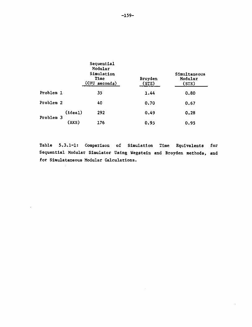
-159-
SequentialModularSimulation
Time(CPU seconds)
Broyden(STE)
SimultaneousModular(STE)
Problem 1
Problem 2
Problem 3
35
40
(ideal)
(RKS)
1.44
0.70
0.49
0.95
292
176
0.80
0.67
0.28
0.95
Table 5.3.1-1: Comparison of Simulation Time Equivalents for
Sequential Modular Simulator Using Wegstein and Broyden methods, and
for Simulataneous Modular Calculations.

-160-
problems where some of the variables in the simulation are required to
be within some imposed bounds (see Section 1.1). Finally, the third
column in Table 5.3.1-1 shows the number of simulation time
equivalents required to solve the problems using the simultaneous
modular concept as implemented in this work.
The most important conclusion that may be drawn from comparing the
number of simulation time equivalents required by each method is that
the simultaneous modular algorithm consistently outperforms the
sequential modular convergence methods. The superior efficiency of the
simultaneous modular simulator is proven over a wide variety of
conditions.
Tables 5.3.1-2 to 5.3.1-5 contain more information about both the
sequential modular and simultaneous modular runs. For sequential
modular calculations, the total number of flowsheet passes (including
the last results pass) and the average time per flowsheet pass. (The
time per pass is larger in the first couple of passes because all the
blocks need to be initialized. Due to the use of retention arrays to
save intermediate results, after the first passes, the blocks are
initialized with the results obtained from the previous pass. This
results in considerable savings in time needed to execute the modules
in a flowsheet pass). For the simultaneous modular runs, the time
spent in each step of the convergence procedure is presented in the
tables. Time measurements are given both in absolute CPU seconds, and
as percentage of the total time needed to converge the flowsheet. The
steps considered in simultaneous modular calculations are the
following:

-161-
(1) Sequential Modular Flowsheet Passes.
(2) Reduced Problem Formulation.
(3) Reduced Problem Solution (the Inside Loop).
(4) Stream Initialization.
The sequential modular flowsheet passes include three basic
operations: flowsheet passes needed to initialize the calculations
(two passes in every problem); execution of the blocks to obtain a
rigorous solution at the beginning of each outside loop iteration (one
flowsheet pass per outside loop iteration), and a last pass (a results
pass) after the flowsheet is converged.
The reduced problem formulation steps include the calculation of
the residuals of the reduced flowsheet equations, and the generation
of the Jacobian matrices associated with the reduced problem
equations. The reduced problem solution steps include only the time
spent in the inside loop solver subroutine. (The operations performed
in this step include the computation of the Newton-Raphson directions
and the variable updates during the convergence of the inside loop).
For Problem 3, the total time needed to initialize the process
streams at the beginning of each outside loop iteration is also
included. By default, only the inlet and tear streams are
reinitialized at each iteration (see Section 2.2). For problems 1 and
2, the stream initialization time is very small and is lumped together
with the time spent in flowsheet passes.
Tables 5.3.1-7 to 5.3.1-10 contain the simultaneous modular
iteration history for each problem. In each of these tables, the left
column is an outside loop iteration counter, while the right column

-162-
Sequential Modular Calculations:
* Number of Flowsheet Passes:
* Time per Flowsheet Pass:
13
2.7 CPU seconds
Simultaneous Modular Calculations - Time distribution:
Step Time Spent (sec) Percent of Total Time
Flowsheet Passes 23.8 82.1%Reduced Problem Formulation 1.1 3.8%Reduced Problem Solution 4.1 14.1%
Table 5.3.1-2: CPU Time Distribution for Benchmark Problem 1.
Sequential Modular Calculations:
* Number of Flowsheet Passes:
* Time per Flowsheet Pass:
16
2.5 CPU seconds
Simultaneous Modular Calculations - Time distribution:
Step Time Spent (sec) Percent of Total Time
Flowsheet Passes 15.6 57.4%Reduced Problem Formulation 1.3 4.6%Reduced Problem Solution 10.3 38.0%
Table 5.3.1-3: CPU Time Distribution for Benchmark Problem 2.

-163-
Sequential Modular Calculations:
* Number of Flowsheet Passes:
* Time per Flowsheet Pass: 7.3 CPU seconds
Simultaneous Modular Calculations - Time distribution:
Time Spent (sec) Percent of Total Time
Flowsheet PassesReduced Problem FormulationReduced Problem SolutionStream Initialization
Table 5.3.1-4: CPU Time Distribution for Benchmark
Ideal Physical Properties.
Sequential Modular Calculations:
* Number of Flowsheet Passes: 16
* Time per Flowsheet Pass:
Problem 3, Using
11.0 CPU seconds
Simultaneous Modular Calculations - Time distribution:
Time Spent (sec) Percent of Total Time
Flowsheet Passes 85.2 50.5%Reduced Problem Formulation 4.0 2.4%Reduced Problem Solution 69.6 41.3%Stream Initialization 9.8 5.8%
Table 5.3.1-5: CPU Time Distribution for Benchmark Problem 3, Using
Redlich-Kwong-Soave Equation-of-State for Physical Properties.
40
Step
34.43.5
40.04.1
42.0%4.3%
48.8%5.0%
Step

-164-
indicates the number of Newton-Raphson iterations needed to converge
the inside loop during each outside loop iteration. At the bottom of
the columns, the total number of outside loop and inside loop
iterations are given.
Several important conclusions may be drawn from the information
given in these tables. The two most time consuming steps in
simultaneous modular calculations are the sequential modular flowsheet
passes and the reduced problem solution. In every case these two steps
account for more than 90 percent of the total time spent in
computations. Thus, it is possible to write the number of simulation
time equivalents (STE) in terms of the number of outside loop
iterations (N0 1), the time per flowsheet pass (Wo) the average
time spent to converge each inside loop subproblem (W i), and the
number of iterations required in sequential modular calculations
(Nsm). Mathematically,
(5.3.1-1) STE - No (W 1o + W i) + 3w01
Nsm ol
This expression may be rewritten as:
(5.3.1-2) STE - N0 + N 0 Wil + constant
No NmWoNsm Nsm Wol
Looking at the terms in the above equation, it is possible to
identify the main factors that influence the performance of
simultaneous modular calculations relative to the standard sequential
modular convergence methodology. It is interesting to note that the
relative efficiency of the simultaneous modular algorithm increases

-165-
(that is, the number of simulation time equivalents decreases) as
either the time per flowsheet pass (W ) or the required number of
sequential modular passes (Nsm) increases. Both of these quantities
are related to the complexity of the flowsheet being simulated.
Chemical processes with complex unit operations will require large
amounts of computer time to simulate the units. Thus, for such
processes, the time needed for each flowsheet pass will also be large.
Similarly, flowsheets with many recycle loops will require more
sequential modular passes to arrive to the converged solution. This
implies that for a given simultaneous modular implementation, the
efficiency of the calculations relative to a sequential modular
simulator will increase as the complexity of the flowsheet increases.
With respect to the parameters in equation (5.3.1-2) which are
related to the simultaneous modular implementation, the number of
outside loop iterations Nol will be problem dependant. Nevertheless,
this quantity will decrease as better reduced models for unit
operations are used. The term better reduced models in this context
means models which approximate better the actual phenomena described
in the rigorous modules. For example, the version of Problem 3
simulated with ideal physical properties required 3 outside loop
iterations to converge. On the other hand, 5 outside loop iterations
were needed when nonideal physical properties were used in the
simulation (see Tables 5.3.1-9 and 5.3.1-10). This difference in
iteration history stems from the fact that the reduced models used for
the inside loop are based to some extent on idealized physical
property equations.
The time needed to converge each inside loop W1 1 be a function

-166-
Sequential Modular Calculations:
* Number of Flowsheet Passes:
* Time per Flowsheet Pass:
40
7.3 CPU seconds
Simultaneous Modular Calculations - Time distribution:
Time Spent (sec) Percent of Total Time
Flowsheet PassesReduced Problem FormulationReduced Problem SolutionStream Initialization
34.33.5
40.09.8
39.2%4.0%
45.7%11.1%
Table 5.3.1-6: CPU Time Distribution for Problem 3, Using Ideal
Physical Properties and Converging all the Stream Variables in the
Outside Loop.
Step

-167-
NUMBER OF ITERATIONS
Outside Loop123456
total: 6
Inside Loop53221
1
Table 5.3.1-7: Iteration History for Problem 1 (Number of Inside
loop Iterations for each Outside Loop Iteration).
NUMBER OF ITERATIONS
Outside Loop Inside Loop1 5234
total: 4
2
11
Table 5.3.1-8: Iteration History for Problem 2 (Number of Inside
Loop Iterations for each Outside Loop Iteration).
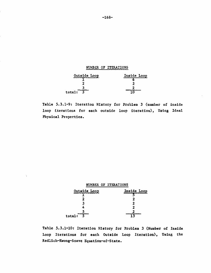
-168-
NUMBER OF ITERATIONS,
Outside Loop123
total: 3
Inside Loop622
10
Table 5.3.1-9: Iteration History for Problem 3 (number of inside
loop iterations for each outside loop iteration), Using Ideal
Physical Properties.
NUMBER OF ITERATIONS
Outside Loop Inside Loop152 23 24 25 2
total: 5 13
Table 5.3.1-10: Iteration History for Problem 3 (Number of Inside
Loop Iterations for each Outside Loop Iteration), Using the
Redlich-Kwong-Soave Equation-of-State.

-169-
of the complexity of the reduced flowsheet equations, the initial
guess provided to converge the reduced equations, and the efficiency
of the numerical algorithm used to solve the inside loop. For the
ideal and nonideal versions of Problem 3, the average times required
to converge each inside loop subproblem are about the same in both
cases (see Tables 5.3.1-4, 5.3.1-5, 5.3.1-9 and 5.3.1-10). Given the
relatively large amounts of time spent solving the inside loop
problems, important improvements in the performance of the
simultaneous modular concept could be achieved if better solution
algorithms were implemented. For example, better sparse matrix
manipulation techniques could lead to important reductions in time
spent in the inside loop.
To test the effect of converging all the streams in the outside
loop versus converging tear and feed streams only, some runs were
carried out using the former implementation. In every case, the
convergence history (number of outside and inside loop iterations) was
the same as when only the tear and feed streams were converged in the
outside loop. However, the amount of time needed to reinitialize all
the streams at the beginning of each outside loop iteration became an
important factor in the overall calculations. For example, table
5.3.1-6 shows the time measurements for the solution of Problem 3 with
ideal physical properties, taking all the stream variables as outside
loop variables. Comparing these results with the ones obtained when
only the tear and feed streams were converged, we observe that the
percentage of total time spent in stream initialization rose from less
than 5 percent to more than 11 percent. For standard simultaneous
modular calculations, it seems more efficient to converge only the

-170-
tear stream variables in the outside loop.
5.3.2 Integrated Simultaneous Modular Calculations
Problems 2 and 3 were used to test the feasibility of integrating
the simultaneous modular calculations with the inside-out algorithm
used for flash calculations in ASPEN PLUS. The two levels of
integration discussed in Section 2.3 were implemented and tested. The
first level of integration, referred as "Integrated Calculations",
corresponds to a case where only one iteration in the inside-out flash
algorithm is performed. The second level of integration, referred as
"Completely Inside-Out Approach", corresponds to the case where the
rigorous model calculations for the flash unit are confined to the
simple model parameter generation.
Integrated calculations converged to the correct solution in all
the test problems. This shows the feasibility of the proposed methods.
For Problem 2, the iteration history (number of outside and inside
loop iterations) obtained with both types of integrated calculations
was exactly the same as for standard simultaneous modular calculations
(see Table 5.3.1-8).
For Problem 3, the iteration history obtained with both types of
integrated calculations was slightly different from that obtained with
standard calculations. Tables 5.3.2-1 and 5.3.2-2 show the number of
inside and outside loop iterations for the ideal and nonideal versions
of Problem 3, respectively. Both types of integration resulted in
identical iteration histories for a given problem. For the version of
Problem 3 simulated with ideal physical properties, the number of

-171-
outside loop iterations was the same as for the case of standard
calculations. However, one less iteration was required to converge the
inside loop during the first outside loop iteration. For the nonideal
version of the problem, the number of outside loop iterations was also
the same with integrated calculations as with standard calculations.
In this case, however, one less inside loop iteration was required
during the last (fifth) outside loop iteration.
Measurements of the CPU time required to converge the benchmark
problems using integrated calculations gave results which were very
similar to the ones obtained from standard calculations. The internal
clock available in the VAX 11/780 computer is not accurate enough to
distinguish between integrated and standard flash calculations (time
measurements varied up to 5% even when the computer had a light load).
For example, Table 5.3.2-3 shows the computation time distribution
obtained when the completely inside-out approach was used on Problem 3
with ideal physical properties. The percentage of the total time spent
in flowsheet passes is very similar to that presented in Table 5.3.1-6
for standard calculations. (In making the comparison between the two
numbers, it should be noted that the percentage of time spent in
flowsheet passes in the completely inside-out case is higher because
less time was spent solving the inside loop). This is not an
unexpected result, given that the problems used to test the concept
are relatively simple. The time savings in the outside loop iterations
resulting from integrated calculations are within the error in the
time measurement. The main savings obtained in the integrated
calculations are derived from the reduced number of inside loop

-172-
iterations. However, this result is problem dependent and may not be
generalized.
There are two important conclusions that may be drawn from the
results obtained by using integrated calculations. The first one is
that the proposed methods are indeed feasible. The second one is
related to the efficiency of the calculations. For the simple problems
used to test the method, the savings in outside loop computations were
much less than the extra work required to converge all the streams in
the outside loop (stream reinitializations at the beginning of the
outside loop iterations). This situation may be expected to change as
the complexity of the units in the flowsheet increases. The main
trade-off for complex flowsheets would be in the extra number of
iterations needed to converge the flowsheet using an integrated
approach (integrated calculations or a completely inside-out
simulator). However, for the problems solved in this work, no increase
in the number of outside loop iterations was observed as a result of
the integrated calculations, which do not require that all the
rigorous models are converged in the outside loop. It should be noted
that when standard simultaneous modular calculations are performed
converging all the stream variables in the outside loop (see Table
5.3.1-6, for example), the overall efficiency of the algorithm is
lower than for the two integrated approaches.
Integrated simultaneous modular approaches seem like a viable way
to further increase the efficiency of simultaneous modular simulators
when dealing with flowsheets that contain complex separation devices.

-173-
NUMBER OF ITERATIONS
Outside Loop123
total: 3
Inside Loop5229
Table 5.3.2-1: Iteration History for Problem 3 (Number of Inside
Loop Iterations for each Outside Loop Iteration), Using Ideal
Physical Properties. Integrated Calculations and Completely
Inside-Out Approach.
NUMBER OF ITERATIONS
Outside Loop Inside Loop1 52 23 24 25 1
total: 5 12
Table 5.3.2-2: Iteration History for Problem 3 (Number of Inside
Loop Iterations for each Outside Loop Iteration) Using the Redlich-
Kwong-Soave Equation-of-State. Integrated Calculations and
Completely Inside-Out Approach.

-174-
Simultaneous Modular Calculations - Time distribution:
Step Time Spent (sec)
Flowsheet Passes 38.5Reduced Problem Formulation 4.2Reduced Problem Solution 41.7Stream Initialization 9.8
Percent of Total Time
40.9%4.5%
44.3%10.3%
Table 5.3.2-3: CPU Time Distribution for Problem 3, Using Ideal
Physical Properties. The Problem is Converged Using a Completely
Inside-Out Approach.

-175-
CHAPTER 6: HANDLING OF DESIGN SPECIFICATIONS
In a standard simulation problem, the process feed streams and the
operating parameters associated with the units are specified by the
user. The solution to the simulation problem gives values for all the
flowsheet variables. For many applications, however, it may be
desirable to supply alternative specifications, which may be any
function of flowsheet variables. For example, the user may want to
specify an output flow rate, or the purity of a product stream, or a
property of any stream other than a process feed. For a simulation
problem, the number of degrees of freedom is always zero; that is, for
each design specification, the user must free a block input variable,
or a process feed stream variable. These manipulated variables would
otherwise be given by the user. The solution of a simulation problem
with design specifications will provide values for the manipulated
variables along with the other flowsheet variables.
When a simulation problem with design specifications is solved
using equation oriented methods, a design specification becomes just
another equation which is added to the original set of flowsheet
describing equations. The problem is then solved in exactly the same
way as a standard simulation problem. At the other extreme, sequential
modular simulators usually create an information recycle loop for each
design specification equation. That is, each design specification adds
another loop that needs to be torn and converged in order to solve the
problem. The additional nesting and coupling of loops makes the

-176-
solution of design problems very inefficient in sequential modular
simulators.
Two-tier simultaneous modular simulators would have both, a
modular step (the outside loop) and an equation oriented part (the
inside loop). The most efficient way to solve a design problem in this
kind of architecture, is to add the design specifications to the
system of equations solved in the inside loop. This would keep the
advantages that equation oriented methods offer for this type of
problem. However, this procedure may not be used directly if the
sampled variables related to the design specifications were eliminated
from the inside loop because of the use of simplified models at this
stage.
The purpose of this chapter is to review the method of solution of
general design specification problems with a simultaneous modular
simulator. A summary of the procedure used in the simulator to handle
manipulated variables is presented in Section 6.1, along with a
discussion of the simple case where all the sampled variables are
included in the inside loop problem. Section 6.2 is devoted to the
case where sampled variables are not present in the reduced problem
but may be introduced by changing the simple 'model for a unit. A
general solution to design specification problems with sample
variables not included in the inside loop is presented in Section 6.3.
Finally, some examples showing the performance of the simultaneous
modular method for design problems are presented in Section 6.4.
-177-
6.1 Handling of Manipulated and Sampled Variables.
Each design specification adds an equation to the reduced problem.
For each added specification, a process variable is freed, so that it
can be adjusted to satisfy the new constraint. In the original
simulation problem, the values of the freed variables (manipulated or
decision variables) were defined by equations that related the
variables with the user's input. When a process variable is freed, the
equation that would set its value should not be generated. The process
of defining decision variables, for simulation or optimization
problems, is simply a mechanism to stop the generation of the
equations that would normally define such variables.
The above statements imply that all the equipment parameters that
may be varied in design or optimization problems need to be included
in the variable list of the inside loop. An equation is generated to
set the numerical value of the parameter in the inside loop (as in
Equation 1.1-2), except when the parameter is freed as a decision
variable. This is also true of the process feed streams, which contain
variables that could be adjusted to achieve certain specifications or
to optimize the flowsheet.
During the transition from the inside loop to the outside loop,
new guesses of the process variables (obtained from the information
gained solving the inside loop) are placed back in the locations
needed for the next round of rigorous modular calculations. These
variables include the equipment parameters which are treated as
decision variables. At this stage, the process streams being converged
in the outside loop (see Sections 2.2.2 and 2.2.3) are reinitialized

-178-
(flashed) to obtain all the stream information needed in the rigorous
models. If there are manipulated variables in the process feed
streams, then these streams should be reinitialized at the start of
the outside loop iterations with the new guesses of the manipulated
variables.
The variables that may be manipulated in design specifications and
optimization problems are usually well identified within each unit,
and they should be considered when a reduced model for the unit is
developed. As long as reasonable reduced models are used in the
two-tier approach, all the manipulated variables will be present in
the reduced problem. This, however, may not be the case with sampled
variables, which may be variables that are not needed to converge the
flowsheet in most simulation problems. For example, internal unit
variables and complex physical properties of streams are eliminated
from the inside loop variable list because they do not need be
computed in the reduced models (see Section 4.1). If all possible
variables were kept in the inside loop, then the resulting calculation
would be equivalent to an equation oriented approach, with all its
disadvantages.
In the simple case when the reduced problem contains all the
sampled variables (and this case covers most design specification
problems found in practice), the design specification equation may be
simply added to the rest of the equations in the inside loop. The
first example presented in Section 6.4 illustrates the performance of
the algorithm in a problem with this characteristic.
The next two sections of this chapter are devoted to the cases
where the sampled variables are not present in the variable list of
the reduced problem.

-179-
6.2 Adaptation of Reduced Models to Introduce Variables.
One of the guidelines suggested for reduced models of process
units (see Chapter 4) is that internal unit variables should be
excluded from the model equations. This way, the number of reduced
simulation equations is automatically reduced. Thus, a simple
nonlinear model for an absorber column, for example, could use
engineering approximations to predict the behavior of the column
without performing stage by stage calculations. In general, there is
no need to compute internal composition and temperature profiles in
the inside loop of the convergence algorithm. However, the possibility
arises that a design specification may be imposed on one of the
internal unit variables that does not appear in the reduced model
equations.
The problem described above is found mainly in staged separation
devices. In this case, the problem may be solved by introducing the
needed variables in the reduced problem through an adaptation of the
reduced model. One approach is to write "smart" simple models that
take different configurations depending upon the problem at hand. For
example, an absorber column for which there is a design specification
on one internal flow could be modelled as two absorber columns
interconnected at the stage where the required internal stream
appears. This idea is illustrated in Figure 6.1. Only two of the
internal streams in the column appear explicitly in the new reduced
model, so as to keep the number of variables in the model as small as
possible. If other internal stream variables had to be accessed, the

-180-
column could be broken in more segments to generate the variables of
interest.
The above approach was discussed in detail in Chapter 4 in
relation to the reduced models for complex distillation columns tested
by Lee [32]. The general idea is to use building blocks to create
reduced models for complex units or to break a unit so as to have
access to internal variables. Each one of the building blocks is in
turn a reduced model for a smaller unit. In the example presented
above, the building blocks are the reduced models for absorption
columns, and two such blocks were used to model one single column in
order to create internal variables needed for design specifications.
For the case of integrated calculations presented in Section 2.3,
the reduced models of most staged separation devices would be the
simple equations used in the two-tier algorithms of the unit operation
blocks. In general, these models include all the internal flowrates
and temperatures; thus, the addition of design specifications on these
variables would pose no additional problems, as the variables would be
already available in the reduced problem.
6.3 Handling of Variables not Present in the Reduced Problem.
For most problems of interest, the addition of the design
specification equations pose no special problems. The sampled
variables most commonly used are already in the inside loop variable
list or may be introduced by an appropriate change in reduced model.
However, a general purpose simulator should be able to solve design
problems for the general case where sampled variables are not in the

-181-
reduced problem.
To handle this case we propose to introduce a "reduced model" to
represent the behavior of the missing sampled variable in the inside
loop. Let us take a design specification of the form:
(6.3-1) h(x,w) = 0
Where x are the process variables included in the inside loop variable
list, and w is a sampled variable eliminated from the inside loop. The
idea is then to introduce the following two equations in the inside
loop:
(6.3-2) w - g(x) - 0
(6.3-3) h(x,w) - 0
The function g(x) is a simple model to represent the behavior of the
sampled variable as a function of the other process variables. With
the addition of the new reduced function, the sampled variable w may
now be introduced to the inside loop variable list. Thus the design
specification equation may now be simply added to the reduced problem.
A simple model for the sampled variable may be a first order
Taylor series expansion of the form:
(6.3-4) w-w aw - ) - w * * 01 xl) - (x2 -x 2 )

-182-
Where x , x2, etc. are the process variables upon which the
sampled variable w depends. The partial derivatives in the above
expression are the simple model coefficients for the linear model.
* *They need to be obtained numerically at the base point (x , w )
during each outside loop iteration, in the same way as the reduced
model parameters for unit operations. Although the number of process
variables in the reduced problem may be quite large for a typical
problem, the number of numerical derivatives to be calculated is in
practice very small. Only the process variables directly associated
with the sampled variable need to be included in the above expression.
Thus, if the sampled variable is a stream variable, only the variables
associated with that stream need to be perturbed to compute partial
derivatives.
6.4 Example Problems.
Three example problems were used to test the performance of the
simultaneous modular simulator for the convergence of flowsheets with
design specifications. All three problems are based on the basic
flowsheet described as Problem 1 in Section 5.1.1. The first
modification to the basic problem tests the performance of the method
for the simple case where the sampled variables in the design
specification equation are included in the inside loop. The second
modification has a design specification on a variable that is not
included in the inside loop. Finally, the third modification to the
basic problem combines both of the design specification equations used
in the other two examples. The purpose of this last problem is to test

-183-
the efficiency of the algorithm as the flowsheet becomes more complex.
The first modification to the original plug-flow reactor problem
to be considered is shown schematically in Figure 6.a. The basic
flowsheet is the same as before, except that a specification is added
to achieve 95% conversion of the reactant A (isobutyric acid) in the
feed. Thus, the specification equation is:
(6.4-1) Afeed - (Aprod + Ableed) - 0.95 - 0
Afeed
Where Afeed, Aprod and Ableed refer to the molar flowrates of
component A in streams FEED, PROD and BLEED, respectively. All the
variables in the above equation are in the inside loop variable list.
To satisfy the above equation, the length of the reactor is to be
varied between a lower limit of 10 meters and an upper limit of 30
meters. The complete report generated by ASPEN PLUS with the results
of the simulation is included in Appendix 5. The length of the reactor
in this case should be 23.3 meters.
The second modification to the problem is shown schematically in
Figure 6.b. The fraction of the liquid stream purged in stream BLEED
is to be varied between 0.005 and 0.6 to achieve a mole fraction of
byproduct G (n-butyric acid) of 0.02 in the stream entering the
reactor (stream REACTIN). The specification equation added to the
original problem is:
(6.4-2) xG,reactin - 0.02 - 0
Although the problem contains one design specification, like the first

MIXER BLOCK
mixeA
______ PUMiP
REACTINptLg- 6ow &eacto&
D P PECPROD
PEC
REACTOUT
10s
RECYCLE
GUNK
Figure 6.a: Plug-Flow Reactor Problem with Design Specification on Conversion.
FEED
1W
00
6 BLEED

MIXER BLOCK
mixeA
______PUMP,
PROD
REACTOUT
6.tazhpeLug-6~tow P4etctot I
SPEC
RECYCLE
00
GUNK
BLEED
Figure 6.b: Plug-Flow Reactor Problem with Design Specification on the MoleFraction of G Entering the Reactor.
FEED
1W
*ft
sptitteA
REACTIN

-186-
problem described above, this example is much more difficult to solve
both in sequential modular and simultaneous modular simulators. In the
first problem, the specification loop solved by the sequential modular
simulator spans only two computation blocks. In the second case, the
specification spans the whole flowsheet. In terms of solution with a
simultaneous modular algorithm, it should be noted that the mole
fractions of the components in a stream are not included in the
reduced flowsheet equations. Therefore the sampled variable
xG,reactin is not directly available in the inside loop variable
list. The method proposed in Section 6.3 needs to be used for the
simultaneous modular solution of the problem. The solution to the
problem is to have 7.3% of the total liquid flow leaving the flash
drum purged in stream BLEED. A complete set of results for this
problem is included in Appendix 5.
The third modification to the problem is indicated in Figure 6.c.
This problem simply adds the two specifications used in the first two
design specification examples to the basic plug-flow reactor
flowsheet, and both the reactor length and the fraction of the liquid
stream purged are treated as decision variables. The solution to this
problem is to use a reactor 31.15 meters long and to purge 48% of the
liquid leaving the flash. A complete set of results is included in
Appendix 5.
All the runs with specifications (both sequential modular and
simultaneous modular) were made using the same run parameters
described in Section 5.2. The initial guess provided for the decision
variables in every case is the value in the basic flowsheet described
in Section 5.5.1 (reactor length - 15.33 meters, split fraction -

(C
MIXER BLOCK
mixeA
pu-fli
p tZow 4acto&L
PROD
PEC
REACTOUT
SPEC
I%RECYCLE
GUNK
BLEED
sptitteA
Figure 6.c: Plug-Flow Reactor Problem with Two Specifications.
FEED
r-
00_jI
REACT IN I

-188-
0.03). The default convergence method provided by ASPEN PLUS (for the
sequential modular runs) for problems with design specifications is to
nest the design specifications inside the tear stream convergence
loops. Thus, two convergence loops were generated by ASPEN PLUS for
the first two problems, and three convergence loops were generated for
the problem with two specifications. The secant method was used to
solve the specification equations, and Wegstein's method was used to
solve the tear stream equations. Although Broyden's method is
available in ASPEN PLUS for the simultaneous solution of tear streams
and design specifications, it was decided not to use this option as a
standard of comparison. Broyden's method is seldom used in practice in
sequential modular simulators due to its unreliability when dealing
with problems with bounds, such as the example problems presented in
this chapter.
A summary of the results obtained for the three example problems
is presented in Table 6.4-1. The first column of this table shows the
number of simulation time equivalents required by ASPEN PLUS (with
sequential modular calculations) to solve each problem. The second
column shows the number of simulation time equivalents required to
solve the same problems using the simultaneous modular algorithm
implemented in this work. (Note that one simulation time equivalent is
referenced to the solution of the flowsheeting problem without
specifications).
Several important conclusions may be drawn from the numbers
presented in the table. The method used to deal with general
specifications which include variables not present in the inside loop
(see Section 6.3) worked successfully for the two test problems in

-189-
Design Spec. on Conversion
Design Spec. on Mole Fraction
Two Design Specifications
STESequentialModular
1.9
4.8
6.4
STESimultaneousModular
0.85
0.84
0.73
Table 6.4-1: Simulation Time Equivalents for Solution of Problems with
Design Specifications.

-190-
this category (the second and the third problems).
In terms of efficiency, the simultaneous modular methodology
proved to be far superior to the sequential modular methods used in
present industrial simulators. As the complexity of the problem
increases, the number of simulation time equivalents required by the
sequential modular version of ASPEN PLUS increases very rapidly. For
the simplest test problem, sequential modular calculations require
twice as much time to converge the flowsheet compared to the basic
flowsheet without specifications. For the more complex example with
one design specification, the number of simulation time equivalents
increases to almost 5. When the two design specifications are imposed
on the basic flowsheet, the number of simulation time equivalents
increases to 6.4. On the other hand, simultaneous modular calculations
seem to be insensitive both to the number and the form (span) of the
specifications. The number of simulation time equivalents is
approximately the same for all cases. In fact, for the test problems
chosen in this chapter, simultaneous modular calculations converge
faster for the more complex cases.
A comparison of the data given in Table 6.4-1 with those presented
in Table 5.3.1-1 suggests that the performance of the simultaneous
modular algorithm for problems with specifications is about the same
as for the solution of the basic flowsheet without specifications. For
all the problems based on the plug-flow reactor flowsheet, the number
of simulation time equivalents required to converge to the solution
was about 0.8. This is not an unexpected result. The design
specifications are solved in the inside loop, which uses an equation
oriented algorithm to converge to the solution. The system of
-191-
equations solved in the inside loop does not change very much with the
addition of the specification equations. Equation (5.3.1-2) was
deribed to predict the number of simulation time equivalents needed to
solve the problem using simultaneous modular calculations as a
function of the complexity of the flowsheet. In terms of this
equation, the number of outside loop iterations (N0 1 ) and the work
needed to solve each reduced problem (W i) remain approximately
constant. Thus, the number of simulation time equivalents is the same
for all the variations of the original problem, even though the
complexity of the flowsheet increases considerably.
Tables 6.4-2 to 6.4-4 show the itertion history and the
computation time distribution for each of the three simultaneous
modular runs (the iteration history for each sequential modular run is
given with the summary of results for the runs in Appendix 5). As
expected, the convergence path and the time distributions are very
similar for all the runs. Since the flowsheet includes a complex unit
which requires a lot of computer time to simulate (the reactor), most
of the time needed to converge the problems using a simultaneous
modular methodology was spent on flowsheet passes. The situation would
be different for a flowsheet with simpler units, as it was shown in
Chapter 5.
It was mentioned in Section 5.3.1 that the relative efficiency of
the simultaneous modular approach increases as the problems become
more complex. Flowsheets with design specifications are good examples
of problems that are difficult to solve in present simulators because
of the added information recycle loops. Using the proposed

-192-
simultaneous modular algorithm, these problems may be handled with the
same degree of efficiency as the basic problems without the design
specifications.

-193-
* Percentage of Time Spent in the Outside Loop: 81.6%
* Percentage of Time Spent in the Inside Loop: 18.4%
NUMBER OF ITERATIONS
Outside Loop Inside Loop122 33 2456
total: 6 12
Table 6.4-2: Iteration History and Time Distribution for Problem 1
with a Design Specification on Conversion.

-194-
* Percentage of Time Spent in the Outside Loop: 86.2%
* Percentage of Time Spent in the Inside Loop: 13.8%
NUMBER OF ITERATIONS
Outside Loop Inside Loop1 52 33 24 15
total: 5 12
Table 6.4-3: Iteration History and Time Distribution for Problem 1
with a Design Specification on Mole Fraction.
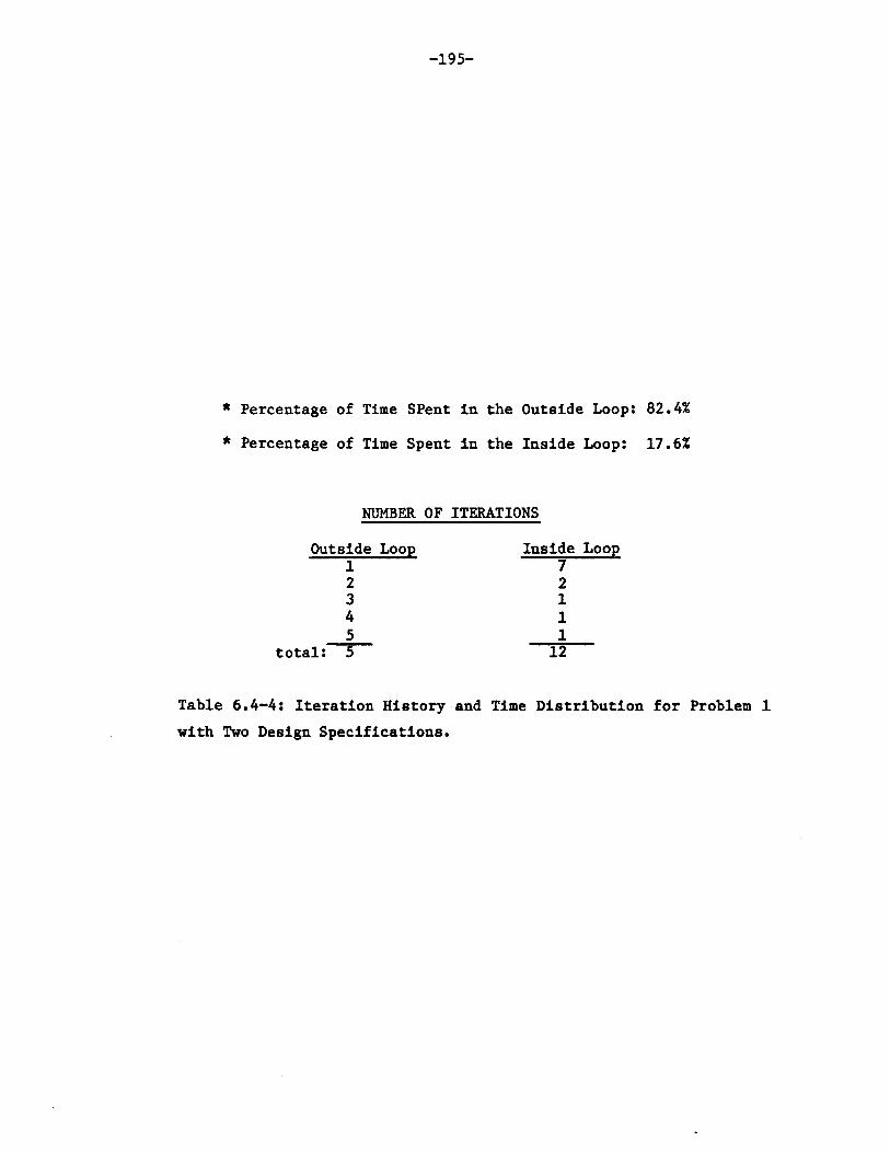
-195-
* Percentage of Time SPent in the Outside Loop: 82.4%
* Percentage of Time Spent in the Inside Loop: 17.6%
NUMBER OF ITERATIONS
Outside Loop12345
total: 5
Inside Loop72111
12
Table 6.4-4: Iteration History and Time Distribution for Problem 1
with Two Design Specifications.