Embed Size (px)
Citation preview

Simultaneous Optimal Design of
Multi-Stage Organic Rankine Cycles
and Working Fluid Mixtures for
Low-Temperature Heat Sources
David M. Thierry1, Antonio Flores-Tlacuahuac∗1 and Ignacio E.
Grossmann2
1Departamento de Ingenierıa y Ciencias Quımicas, Universidad Iberoamericana,
Prolongacion Paseo de la Reforma 880, Mexico D.F., 01219, Mexico.
2Department of Chemical Engineering, Carnegie-Mellon University,
5000 Forbes Av., Pittsburgh 15213, PA
October 26, 2015
∗Author to whom correspondence should be addressed. E-mail: [email protected],phone/fax:+52(55)59504074, http://200.13.98.241/∼antonio
1

Abstract
Energy recovery is a process strategy seeking to improve process efficiency through
the capture, recycle and deployment of normally neglected low energy content
sources or streams. By proper optimal process design, such low-temperature en-
ergy sources can be a feasible and economical manner of approaching the energy
recovery issue. In particular, when Rankine cycles with mixtures as working fluids
are used, the amount of energy recovery can be improved. The formulation and
systematic solution of this problem has shown better results when all the variables
of the Rankine cycle and the compositions of the working fluid are considered simul-
taneously. Another interesting approach is the implementation of multiple cycles
coupled together. In this work we propose a nonlinear optimization formulation of
two general multistage approaches for the Rankine cycle with mixtures: the cascade
and series configurations. As main decision variables, we have considered the heat
source conditions and the mixture components. Then, the resulting optimization
problem is solved in a deterministic approach as a nonlinear program. The results
shown that for some cases the multistage configurations are useful but limited in
terms of cost in comparison to the single stage cycle.
2

1 Introduction
The generation of energy with low-environmental cost technologies is an important matter
that has been continuously assessed over the years. One particular appealing idea is
conversion of low-temperature heat to power by means of an Organic Rankine Cycle
(ORC) [1, 2]. The performance of the ORC can be improved by several strategies, like
modifications of the cycle configuration, pure and mixture working fluids selection and
design. Linke et al. [3] performed an in depth review of the state of the art systematic
methods for the ORC design.
Recent approaches on the selection and design of the working fluid, either pure or mix-
ture include the following works. Mavrou et al. [4] investigated the selection of working
fluid mixtures through sensitivity analysis; their framework enabled them to identify the
operating parameters whose variation impacted the ORC performance the most, and the
mixture which has the best performance under variable conditions. Braimakis et al. [5] in-
vestigated several pure fluids and binary mixtures with both sub-critical and supercritical
operations. They found that the supercritical ORC with low critical temperature fluids
and moderate to high heat source temperatures displays an increase of exergetic efficiency.
Lampe et al. [6] created a framework for the simultaneous selection of the working fluid
and process optimization through a continuous molecular targeting approach. They were
able to identify the best performing fluids from a large database. Lecompte et al. [7]
presented an overview of the ORC architectures.
A relevant work on the simultaneous mixture and operating conditions selection by
means of nonlinear optimization was previously presented [8]. In this work a nonlinear
model was developed and solved for a set of case studies. It was found that optimal
mixtures only require a few components; forcing additional species into the mixture does
not improve the efficiency of the cycle.
As part of the cycle configuration approaches, the multistage concept has been devel-
3
oped by various authors with a number of configurations. The basic idea is to consider
several pieces of equipment, so more power is generated or a less costly scheme is obtained.
In this regard, Kosmadakis et al. [9] carried out an economic assessment of a two-stage
Solar Organic Rankine Cycle that drives an desalinization unit. The evaluated cycle in
this paper is in a cascade configuration, and showed a better efficiency and lower specific
cost than a single-stage. Morisaki et al. [10] introduced a formula for the calculation
of the maximum power of a multistage heat engine (which is the basic idea of the series
configuration in this work). They found that the multi-stage configuration doubled the
power in comparison to the single-stage, although the efficiency is constant regardless
the number of stages. Yun et al. [11] evaluated an experimental ORC with multiple
expanders that works in parallel. They found the multiple expander design is better
than the basic-ORC when they are subject to large variations in the amounts of waste
heat produced. Li et al. [12] evaluated the performance of two configurations of ORCs
where the heat source is segmented into two temperature ranges. They found that the
series configuration has better performance than the parallel cycle. Stijepovic et al. [13]
developed a mathematical model based on the exergy composite curves for the analysis
of ORCs with a multi-pressure configuration. Then, they implemented an optimization
strategy that determined the number of pressure loops and operating parameters.
The potential of simultaneous multiple Rankine cycles is generally recognized, al-
though there are many different configurations, it is necessary to develop a generic scheme
of multistage ORCs and to draw a conclusion on the improvements.
Additionally, the design of the working fluid mixtures for this kind of configurations
has not been addressed. It is possible to implement an individual mixture for each stage,
and have stages absorbing heat in various ways. With this, it is also possible to compare
the cost implications of these configurations and draw a conclusion on their potential.
Therefore, in this work we propose the extension of ORCs with mixtures to multistage
configurations, all developed with an equation oriented approach, meaning that every
4
aspect from thermodynamics to cost constraints are included and solved simultaneously
in a nonlinear optimization model. To our best knowledge, such a problem has not been
considered in the open research literature.
2 Problem Definition
The appropriate selection of the operating conditions and mixture composition is a way
of increasing the efficiency of the power generation of the Rankine Cycle (RC) with low-
temperature heat sources. But even in the most efficient RC, heat rejection is considerable
and unavoidable. Because we are still far from the upper limit imposed by the thermo-
dynamics, it is reasonable to assume that by absorbing more heat by means of a more
complex scheme, the efficiency of the cycle would be better than that achieved by the
simple RC.
A natural way of trying to absorb more heat than in a single RC would be using a
second cycle at the same time. How the second RC should be coupled with the heat
source is a more complicated issue if we consider that there is no unique way of doing
this. A single RC takes heat from the heat source (HS) in the vaporizer (Figure 1). We
could partition the HS stream and send the resulting streams to an individual RC (in this
case two HS streams two RCs). If we recognize that the HS heat content could also be
partitioned, then every part of the heat could be used in a RC. This is the idea of the
series-connected RC (Figure 2). The main difference between these two processes is that
the first one is a physical split of the HS stream, while the second is an energy split.
If we try to find the optimal operating conditions from the above stated configurations,
we would find that only the second one (i.e. the Series RC) matters, because if we set-
up a molar basis model the solution of the first one would be two identical cycles (or
the single cycle solution). Also, the second problem would be the determination of the
optimal operating conditions and the composition of the working fluid mixtures for each
5

High Pressure Level
Low Pressure Level
Vaporizer
Condenser
Pump
Turbine
1
Heat source (HS)
Heat sink (CS)
2
3
4
Figure 1: The Rankine Cycle
Heat source (HS)
Heat sink (CS) Heat sink (CS)
s=1 s=2
Figure 2: Two-stage Series flow diagram
6

cycle simultaneously.
Other possible configuration revolves around the fact that every individual RC has to
reject heat. A second cycle can take the rejected heat from the first cycle and then to
generate power from it. This succession ends in the rejection of heat to the sink by the
second cycle and is the basic idea of the Cascade configuration is shown in Figure 3.
Heat source (HS)
Heat Sink (CS)
s=1
s=2
Figure 3: Two-stage Cascade flow diagram
Every consecutive cycle in the Cascade configuration would have to absorb a smaller
amount of heat, and possibly minimize the heat rejection. The two configurations of
multiple RCs can be further generalized as shown by the Figures 4 and 5, where a large
number of cycles can be implemented.
Naturally we can expect some impact on the efficiency of the overall cycle. But it is
also important to consider the economic implications in terms of what these configurations
do to the price that we have to pay for the electricity produced. This is why the sizing
of the equipment becomes a necessity. With all this information comprised into a model,
7

RC RC
HS
CS CSCS
SLast1 RC2
Figure 4: The series configuration, a heat flow from Source (HS) to Rankine cycles (RC)and to the Heat Sinks (CS).
we can make decisions on the mixtures that are used as working fluids, and the operating
conditions at which the cycle is carried out.
Assuming that several sources of low-temperature heat are available, and that maxi-
mum heat recovery (trough power generation) is desired, then, there are two key elements
that we can exploit to achieve this goal: (a) a set of multistage series/cascade Rankine
cycles with variable pressures, temperatures, flows, etc.; and (b) a working fluid that is
mixture of a set of predefined components suitable for the low-temperature application
with variable composition.
The problem to be addressed in this work can be stated as follows: “For a given low-
temperature heat source the problem consists in simultaneously obtaining the optimal
mixture composition of the working fluid from some predefined components, and the
optimal operating conditions of a set of series or cascade coupled Rankine cycles such
that to maximum energy recovery or minimum electricity cost are achieved”.
8

RC
RC
HS
CS
1
SLast
RC2
Figure 5: The cascade scheme. Heat flow from Heat Source (HS) through Rankine cycles(RC) to the Heat Sink (CS)
9

3 Optimization Formulation
3.1 Sets
The sets required for the algebraic formulation of the problem are defined as follows:
• The Available chemical species i, j ∈ I
• The stage s ∈ STG = 1, 2, .., SL; if the cycle is single stage then STG = 1.
• The UNIFAC functional group k,m, n ∈M related to the activity coefficients.
• The phase f ∈ F = Liquid(L),Vapor(V) , for calculations that are for a particular
phase.
• The equilibrium or two phase point π ∈ Π = Bubl,1,2,3,..,Dew (1,2,3, are internal
points between bubble and dew point).
• The pressure level p ∈ L = High,Low , which relates to its location in the cycle.
• The subcool o ∈ O=Sub,SubS and superheat (nonisentropic,isentropic) o ∈ O =Over,OverS
; O ∪ O = O. Which imply variables that are not at equilibrium and are exclusive
for single phase.
Moreover, it should be noted that there are two main groups of variables, the off-
superheat/subcool and the on-superheat/subcool (denoted with the index o).
The optimization algebraic models are summarized in Figure 7. The equations are
distributed in four main groups: (1) the equation of state group Zs which contains infor-
mation related to the compressibility factors; (2) the activity coefficients Gs which contain
the core of the UNIFAC method of activity coefficients; (3) the equilibrium and property
set Bd which contains the enthalpy, entropy, fugacity and equilibrium relationships; and
(4) the ϕs constraints that are comprised of the isentropic, nonisentropic, heat and work
10
Vapor
Two-P
hases
Liqu
id
p=High
p=Low
T
S
f =LiquidTwo-phasef =Vapor=Bubble =Dew =2-phaseo=Subo=SubSo=Overo=OverS
3
4
2
1
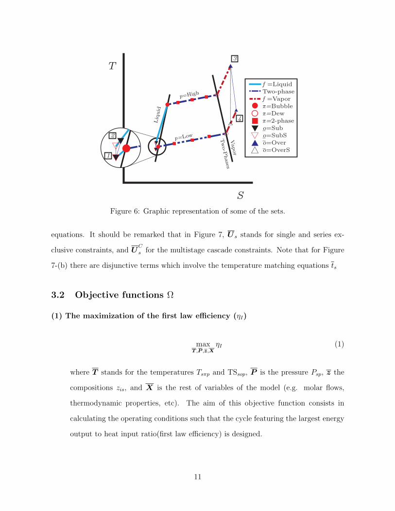
Figure 6: Graphic representation of some of the sets.
equations. It should be remarked that in Figure 7, U s stands for single and series ex-
clusive constraints, and UC
s for the multistage cascade constraints. Note that for Figure
7-(b) there are disjunctive terms which involve the temperature matching equations ts
3.2 Objective functions Ω
(1) The maximization of the first law efficiency (ηI)
maxT ,P ,z,X
ηI (1)
where T stands for the temperatures Tsπp and TSsop, P is the pressure Psp, z the
compositions zis, and X is the rest of variables of the model (e.g. molar flows,
thermodynamic properties, etc). The aim of this objective function consists in
calculating the operating conditions such that the cycle featuring the largest energy
output to heat input ratio(first law efficiency) is designed.
11

maxT ,P ,z,X
Ω
s. t. Zs
(P s,T s, zs,Xs
)= 0
Gs
(P s,T s, zs,Xs
)= 0
Bd
(P s,T s, zs,Xs
)= 0
ϕs
(P s,T s, zs,Xs
)≤ 0
Cs
(P s,T s, zs,Xs
)= 0
U s
(P s,T s, zs,Xs
)≤ 0
P s,T s ≥ 00 ≥ zs ≥ 1
P s,T s, zs,Xs ∈ Rn
s ∈ STG
(a)
maxT ,P ,z,X
Ω
s. t. Zs
(P s,T s, zs,Xs
)= 0
Gs
(P s,T s, zs,Xs
)= 0
Bd
(P s,T s, zs,Xs
)= 0
ϕs
(P s,T s, zs,Xs
)≤ 0
Cs
(P s,T s, zs,Xs
)= 0
UC
s
(P s,T s, zs,Xs
)≤ 0(
Y liqs
tLs (liq) = 0
)∨
(Y 2Ps
tLs (2P) = 0
)(
Y vaps
tUs (vap) = 0
)∨(
Y 2Ps
tUs (2P) = 0
)Y liqs ∨Y 2P
s
Y vaps ∨Y 2P
s
P s,T s ≥ 00 ≥ zs ≥ 1
P s,T s, zs,Xs ∈ Rn
Y liqs , Y 2P
s , Y vaps , Y 2P
s ∈ true,false
s ∈ STG
(b)
Figure 7: Model for the mixture-ORC (a) Single stage (U s = U1
s, s = 1), and multi-stage
series (U s = US
s , s ∈ STG). (b) Cascade multi-stage
12

(2) The minimization of the cost per annual MWh (C)
minT ,P ,z,X
C (2)
This objective function is the ratio between the updated base cost of the cycle plus
the overall utilities over its whole lifespan, and the electricity produced in a year (see
eq. 184). The aim of using this objective function is to design a cycle whose cost
is justified through its energy production. In other words, it implies that whatever
cycle is obtained, it would be the one what has the less costly power generation
accounting for the operation and fixed cost of the cycle itself.
3.3 Constraints
(1) Equations of state Zs
(T s,P s, zs
)= 0
A large part of the algebraic model is used to describe the thermodynamics of the cycle
by means of equations of state (EOS). The EOS are used in two main forms: for pure
components and for mixtures. The thermodynamic behavior of the pure components was
described with the Soave-Redlich-Kwong equation of state (SRK) [14]. For mixtures,
the Predictive-SRK equation of state (PSRK) [15] was used. This last equation is an
extension of the SRK equation for a mixture, with the activity coefficients as part of a
mixing rule.
Regarding the notation used in this work, some variables are exclusive of pure com-
ponents like the temperature functions (fT )isπp or αisπp, while others are only related to
the mixture like αsπp or αisπp. Additionally, the notation of the equation definitions are
simplified. The equations in the form: “variablesindexes =expression” are always defined
over: “indexes∈Set” (e.g. Eq. 3 with i ∈ I, s ∈ STG, π ∈ Π, p ∈ L), except when is
explicitly stated in the equation (e.g. i ∈ I, s ∈ STG, π ∈ Π, p ∈ L).
13

The temperature function variables from the SRK EOS for pure at equilibrium, refer-
ence and superheat temperatures are as follows:
(fT )isπp =[1 + cω,i
(1− (Tsπp/Tci)
0.5)]2 (3)
(fRT )isp =[1 + cω,i
(1− (TRFisp/Tci)
0.5)]2 (4)
(fST )isop =[1 + cω,i
(1− (TSsop/Tci)
0.5)]2 (5)
where Tsπp,TRFisp, and TSsop are the equilibrium, reference and superheat temperatures.
cω,i are the acentric parameters and Tci are the critical temperatures. The variables for
the EOS polynomial are given by the following equations:
αisπp =0.42748RgTc2i (fT )isπp
PcibiTsπp(6)
aRisp =0.42748RgTc2i (fRT )isp
PcibiTRFisp(7)
aSisop =0.42748RgTc2i (fST )isop
PcibiTSsop(8)
βsatisπp =
biPsatisπp
RgTsπp(9)
bRisp =biPsp
RgTRFisp(10)
where P satisπp is the saturation pressure, Rg is the gas constant, Pci is the critical pressure
and bi is a pure component parameter. The corresponding mixture variables are the
following:
bsπp =∑i∈I
xisV πpbi (11)
βsπp =bsπpPspRgTsπp
(12)
14
bSsop =bs,Dew,pPspRgTSsop
(13)
where xisV πp is the equilibrium vapor phase composition and Psp is the cycle pressure.
The PSRK (Predictive-SRK) mixing rule involves the compositions and the Gibbs excess
energy of the mixture GsπV p (and GSsop for superheat) given by the activity coefficients.
αsπp = − 1
0.64663
(GsπV p +
∑i∈I
xisV πp lnbsπpbi
)+∑i∈I
xisV πp(αisπp) (14)
aSsop = − 1
0.64663
(GSsop +
∑i∈I
zis lnbs,Dew,p
bi
)+∑i∈I
zis(aSisop) (15)
Considering that aSsop is at nonphase-equilibrium conditions, the global composition zis
is then used. Also the molar partial variable is given by,
αisπp =1
A1
(ln γisπV p + ln
βsπpβi
+βisπp
βsπp− 1
)+ αisπp (16)
where ln γisπV p is the activity coefficient with the composition of the vapor phase and A1 is
a parameter. Next, the constraints that are related to the compressibility factor variable
are cubic polynomials. Each one of these constraints is related to a required state, namely
pure saturation, reference temperature, mixture at equilibrium and nonequilibrium.
(Zsatisπp
)3 − (Zsatisπp
)2+[−βsat
isπp −(βsatisπp
)2+ αisπpβ
satisπp
]Zsatisπp − αisπp
(βsatisπp
)2= 0
i ∈ I, s ∈ STG, π ∈ Π, p ∈ L(17)
(ZRisp)3 − (ZRisp)
2 +[−bRisp − (bRisp)
2 + aRispbRisp
]ZRisp − aRisp (bRisp)
2 = 0,
i ∈ I, s ∈ STG, p ∈ L(18)
(Zsπp
)3−(Zsπp
)2+
[−βsπp −
(βsπp
)2+ αsπpβsπp
]Zsπp − αsπp
(βsπp
)2= 0,
s ∈ STG, π ∈ Π, p ∈ L(19)
15

(ZSsop
)3−(
ZSsop
)2+
[−bSsop −
(bSsop
)2+ aSsopbSsop
]ZSsop − aSsop
(bSsop
)2= 0,
s ∈ STG, o ∈ O, p ∈ L
(20)
where Zsatisπp,ZRisp, Zsπp and ZSsop are the respective compressibility factors. It should be
noted that because the previous equations are cubic polynomials, more than one root
is expected. Only one is useful for our purposes (i.e. the vapor root). Therefore, we
require a way of discerning which of the roots are we obtaining at the same time that the
problem is being solved. This is problematic; however a simple yet convenient method
for dealing with this issue is by adding the two constraints introduced in [16]. These two
constraints involve the first and second derivatives of the previous equations. Then, the
first derivative constraints are:
3(Zsatisπp
)2 − 2Zsatisπp +
[−βsat
isπp −(βsatisπp
)2+ αisπpβ
satisπp
]≥ 0,
i ∈ I, s ∈ STG, π ∈ Π, p ∈ L(21)
3(Zsπp
)2− 2Zsπp +
[−βsπp −
(βsπp
)2+ αsπpβsπp
]≥ 0,
s ∈ STG, π ∈ Π, p ∈ L(22)
3 (ZRisp)2 − 2ZRisp +
[−bRisp − (bRisp)
2 + aRispbRisp
]≥ 0,
i ∈ I, s ∈ STG, p ∈ L(23)
3(
ZSsop
)2− 2ZSsop +
[−bSsop −
(bSsop
)2+ aSsopbSsop
]≥ 0,
s ∈ STG, o ∈ O, p ∈ L(24)
And the second derivative constraints:
6(Zsatisπp
)− 2 ≥ 0, i ∈ I, s ∈ STG, π ∈ Π, p ∈ L (25)
16

6(Zsπp
)− 2 ≥ 0, s ∈ STG, π ∈ Π, p ∈ L (26)
6 (ZRisp)− 2 ≥ 0, i ∈ I, s ∈ STG, π ∈ Π, p ∈ L (27)
6(
ZSsop
)− 2 ≥ 0, s ∈ STG, o ∈ O, p ∈ L (28)
These equations collectively will allow us to obtain an appropriate root for the compress-
ibility factor.
(2) Activity Coefficients Gs
(T s,P s, zs,X
)= 0
The versatility of the UNIFAC [17] method makes it appropriate for this model, since it
does not require pure component experimental information, just the binary interaction
parameters for each functional group pair in the mixture, and two additional parameter
for each group. The only disadvantage is that it depends on binary interaction parameters
amn.
The following equations are the core of the UNIFAC activity coefficients model.
ln γisπfp = ln γCisπfp + ln γRisπfp (29a)
ln γCisπfp = lnri∑
j∈Irjxjsπfp
+10
2qi ln
qi∑j∈I
rjxjsπfp
ri∑j∈I
qjxjsπfp+ li −
ri∑j∈I
rjxjsπfp
∑j∈I
xjsπfplj (29b)
ln γRisπfp =∑k∈M
νik (ln Γksπfp − lGPiksπp) (29c)
lGPiksπp = Qk
1− ln
(∑m∈M
TPimΨmksπp
)−∑m∈M
TPimΨkmsπp∑n∈M
TPinΨnmsπp
(29d)
ln Γksπfp = Qk
1− ln
(∑m∈M
θmsπfpΨmksπp
)−∑m∈M
θmsπfpΨkmsπp∑n∈M
θnsπfpΨnmsπp
(29e)
17

θmsπfp =QmXmsπfp∑
n∈MQnXnsπfp
(29f)
Ψmnsπp = exp
(− amnTsπp
)(29g)
Xmsπfp =
∑i∈Ixisπfpνim∑
i∈I
(xisπfp
∑n∈M
νin
) (29h)
The required parameters are:
ri =∑k∈M
νikRk (30a)
qi =∑k∈M
νikQk (30b)
li =10
2(ri − qi)− (ri − 1) (30c)
TPim =QmXPim∑
n∈MQnXPin
(30d)
XPim =νim∑
n∈Mνin
(30e)
where νim is the group frequency, amn [18] is the binary interaction parameter, Rk and
Qk are group parameters. We only display the group for UNIFAC once, but in fact the
equations are required one second time with the temperature TSsop. Also, through this
work, the temperature derivatives of the activity coefficient are required. But they only
involve the temperature dependent variables, namely the equations with Ψmnsπp. We will
not show them but the derivation is straightforward and can be found elsewhere [19].
18

(3) Equilibrium and Property constraints Bs
(T s,P s, zs,X
)= 0
(a) Equilibrium. The equilibrium constraints consist of equalities involving fugacity
coefficients, K-value and the Rachford-Rice equation. These equations are only defined
for the two-phase region of the cycle, i.e. inside the heat exchangers. First, the fugacity
coefficient constraints are defined for the pure species at saturation pressure and the
mixture at equilibrium temperature [20].
(ln Φsat
)isπp
= Zsatisπp − 1− ln
(Zsatisπp − βsat
isπp
)− αisπp ln
(Zsatisπp + βsat
isπp
Zsatisπp
)(31)
(ln Φ
)isπp
=bi
bsπp
(Zsπp − 1
)− ln
(Zsπp − βsπp
)− αisπp ln
(Zsπp + βsπp
Zsπp
)(32)
The K-value or equilibrium ratio as given here assumes incompressible liquids. Also the
inclusion of the activity coefficient of the liquid phase (ln γisπLp) has to be noted:
Kisπp =exp (ln γisπLp)P
satisπp exp (ln Φsat)isπp
exp(
ln Φ)isπp
Psp(33)
Regarding the Rachford-Rice equation [21] a re-arranged version of the equation was used
because the original form is prone to becoming undefined during the solution process:
∑i∈I
(zis
1 + ψπ (Kisπp − 1)
∏j∈I
(1 + ψπ (Kjsπp − 1))
)= 0
s ∈ STG, π ∈ Π, p ∈ L
(34)
where ψπ is the vapor phase ratio. With the equilibrium constraints now defined, the last
constraints are the mole fraction of the vapor, liquid and consistency equations. For the
liquid phase:
xisLπp =zis
(1 + ψπ (Kisπp − 1))(35)
19

whereas for the vapor phase:
xisV πp =zisKisπp
(1 + ψπ (Kisπp − 1))(36)
and the summations consistency equations:
∑i∈I
zis = 1, i ∈ I (37)
∑i∈I
xisfπp = 1, i ∈ I, s ∈ STG, π ∈ Π, p ∈ L (38)
(b) Property. The property section of the model deals with the constraints for the
vapor pressure, reference temperature, enthalpy and entropy; these last two being the
most important because they allow us to know the thermodynamic states over the cycle
and the overall energy inputs and outputs.
The vapor pressure (or saturation) and the reference temperature are each one given by
the extended Antoine equation [22]:
lnP satisπp = C1,i −
C2,i
Tisπp + C3,i
+ C4,iTisπp + C5,i lnTisπp + C6,iTC7,i
isπp (39)
lnPsp = C1,i −C2,i
TRFisπp + C3,i
+ C4,iTRFisπp + C5,i ln TRFisπp + C6,iTRFC7,i
isπp (40)
The first equation gives the saturation pressure P satisπp for the equilibrium temperature
Tisπp, whereas the second one gives the reference temperature TRFisπp for the pressure
of the cycle Psp. Moreover, C1,i through C7,i are parameters for the pure species. These
parameters were taken from the Aspen Plus property data [23].
The enthalpy and entropy are established for the liquid and vapor phases through the
residuals (or departures from ideal gas), ideal gas and liquid changes, and the latent heat.
First, the residuals require temperature derivatives of the parameters used in the EOS
20
section.
(f ′T )isp = − cω,iTci
[1 + cω,i
(1− (Ts,Dew,p/Tci)
0.5)](Ts,Dew,p
Tci
)−0.5(41)
(fR′T )isp = − cω,iTci
[1 + cω,i
(1− (TRFisp/Tci)
0.5)](TRFispTci
)−0.5(42)
(fS′T )isop = − cω,iTci
[1 + cω,i
(1− (TSsop/Tci)
0.5)](TSsopTci
)−0.5(43)
aR′isp = 0.42748 (fR′T )isp (44)
a′isp = 0.42748 (f ′T )isp (45)
aS′isop = 0.42748 (fS′T )isop (46)
The temperature derivatives of the mixture variables are related to the Gibbs excess
energy derivatives G′sp and GS′sop.
a′sp =G′spA1
+
(∑i∈I
zisa′ispbi
R2gTc2iPci
)+Rg
A1
∑i∈I
zis ln
(bs,Dew,p
bi
)(47)
aS′sop =GS′sop
A1+
(∑i∈I
zisaS′isopbi
R2gTc2iPci
)+Rg
A1
∑i∈I
zis ln
(bs,Dew,p
bi
)(48)
The enthalpy ((HR)sp,HRRFisp and (HR)sop) and entropy (
(SR)sp, SRRFisp and (SR)sop)
residual equations [20] are defined for assessing the phase equilibrium behavior, the ref-
erence state and the superheat states. Enthalpy:
(HR)sp
= −(αs,Dew,p −
a′spRg
)ln
Zs,Dew,p
Zs,Dew,p + βs,Dew,p
+ 1− Zs,Dew,p (49)
HRRFisp = −
(aRisp −
aR′ispRgTc2iPcibi
)ln
ZRisp
ZRisp + bRisp
+ 1− ZRisp (50)
(HR)sop = −(
aSsop −aS′sopRg
)ln
ZSsop
ZSsop + bSsop+ 1− ZSsop (51)
21

Entropy:
(SR)sp
= − ln(Zs,Dew,p − βs,Dew,p
)+a′s,Dew,p
Rg
lnZs,Dew,p
Zs,Dew,p + βs,Dew,p
(52)
SRRFisp = − ln (ZRisp − bRisp) +aR′ispRgTc2i
Pcibiln
ZRisp
ZRisp + bRisp
(53)
(SR)sop = − ln(
ZSsop − βs,Dew,p
)+
aS′sopRg
lnZSsop
ZSsop + bSsop(54)
Note that the residuals are given in terms of temperature derivatives of the SRK and
PSRK variables and the compressibility factor. For the definition of the properties we
also need the ideal gas changes. Both use equations with parameters fitted from the
integrated form of an equation used in [8]. This leaves consistently simple equations,
although the accuracy of the predicted change values is reduced. Once again three states
are evaluated, so three equations for each property are required.
Enthalpy:
Hu(DHRid
)isp
=
cpx1i3
[(TRFisp)
3 − 298.153]
+cpx2i
2
[(TRFisp)
2 − 298.152]
+ cpx3i [TRFisp − 298.15]
(55)
Hu(∆H id
)isp
=
cpx1i3
[(Ts,Dew,p)
3 − 298.153]
+cpx2i
2
[(Ts,Dew,p)
2 − 298.152]
+ cpx3i [Ts,Dew,p − 298.15]
(56)
Hu (∆Hs)isop =
cpx1i3
[(TSsop)
3 − 298.153]
+cpx2i
2
[(TSsop)
2 − 298.152]
+ cpx3i [TSsop − 298.15](57)
22

Entropy:
Su(sTRid
)isp
=
cpx1i2
[(TRFisp)
2 − 298.152]
+ cpx2i [TRFisp − 298.15] + cpx3i [ln (TRFisp)− ln 298.15]
(58)
Su(∆Sid
)isp
=
cpx1i2
[(Ts,Dew,p)
2 − 298.152]
+ cpx2i [Ts,Dew,p − 298.15] + cpx3i [ln (Ts,Dew,p)− ln 298.15]
(59)
Su (∆Ss)isop =
cpx1i2
[(TSsop)
2 − 298.152]
+ cpx2i [TSsop − 298.15] + cpx3i [ln (TSsop)− ln 298.15](60)
where the parameters cpx1i through cpx3i are reported in the results section. It has to be
noted that the parameters Hu and Su were also added as scaling factors in all enthalpy
equations. We also implemented this last technique for the liquid property changes. This
time the pure parameters cpl1i to cpl3i were used. Enthalpy:
Hu (∆Hlisp) =
cpl1i3
[(Ts,Bubl,p)
3 − TRF3isp
]+
cpl2i2
[(Ts,Bubl,p)
2 − TRF2isp
]+ cpl3i [Ts,Bubl,p − TRFisp]
(61)
Hu (∆HlSisop) =
cpl1i3
[(TSsop)
3 − TRF3isp
]+
cpl2i2
[(TSsop)
2 − TRF2isp
]+ cpl3i [TSsop − TRFisp]
(62)
23

Entropy:
Su (∆Slisp) =
cpl1i2
[(Ts,Bubl,p)
2 − TRF2isp
]+ cpl2i [Ts,Bubl,p − TRFisp] + cpl3i [ln (Ts,Bubl,p)− ln TRFisp]
(63)
Su (∆SlSisop) =
cpl1i2
[(TSsop)
2 − TRF2isp
]+ cpl2i [TSsop − TRFisp] + cpl3i [ln (TSsop)− ln TRFisp]
(64)
Only two states for the liquid phase are needed (i.e. equilibrium and nonequilibrium).
Reference vaporization enthalpy (latent heat) equation through the Watson equation [14]:
(DhRlv
)isp
= ∆hBLVi
(1− TRFisp/Tci
1− Tbri
)0.375
(65)
Those constraints lead to the definition of the molar properties. In the case of the liquid
phase, start from the formation enthalpy and Gibbs free energy (DHFi and DGFi) of the
pure species at ideal gas state with 298.15 K and 1 atm. Then the changes go from pure
ideal to real gas, pressure correction, condensation at the reference temperature, ideal
liquid solution to real liquid solution, and liquid change to the final temperature (Ts,Bubl,p
or TSsop). All these steps of calculation are embedded in the following 4 equations for the
liquid phase enthalpy and entropy.
Enthalpy:
hsp =∑i∈I
zis
[DHFi
Hu+(DHRid
)isp− 8.314
HuTRFispHRRFisp −
(DhRlv
)isp
+ ∆Hlisp
](66)
hSsop =∑i∈I
zis
[DHFi
Hu+(DHRid
)isp− 8.314
HuTRFispHRRFisp −
(DhRlv
)isp
+ ∆HlSisop
](67)
24

Entropy:
ssp =∑i∈I
zis
[DHFi −DGFi
Su · 298.15+(sRid
)isp− 8.314
Su
[ln
(Psp
1.01325
)+ SRRFisp
]− Hu
Su
(DhRlv
)isp
TRFisp+ ∆Slisp
](68)
sSsop =∑i∈I
zis·[DHFi −DGFi
Su · 298.15+(sRid
)isp− 8.314
Suln
(Psp
1.01325
)+
8.314
SuSRRFisp −
Hu
Su
(DhRlv
)isp
TRFisp+ ∆SlSisop
](69)
The vapor phase properties follow a shorter trajectory, from ideal gas at 298.15 K and 1
atm, ideal gas change, pressure change, and ideal gas mixture to real gas mixture. The
gas enthalpy is given by:
Hsp =∑i∈I
zis
[DHFi
Hu+(∆H id
)isp
]−(HR)spTs,Dew,p
8.314
Hu(70)
HSsop =∑i∈I
zis
[DHFi
Hu+ (∆Hs)isop
]− (HR)sop TSsop
8.314
Hu(71)
while the gas entropy by,
Ssp =∑i∈I
zis
[DHFi −DGFi
Su · 298.15+(∆Sid
)isp− 8.314
Suln
(Psp
1.01325
)]−(SR)sp
8.314
Su(72)
SSsop =∑i∈I
zis
[DHFi −DGFi
Su · 298.15+ (∆Ss)isop −
8.314
Suln
(Psp
1.01325
)]− (SR)sop
8.314
Su(73)
It should be noted that the units of the enthalpy and entropy are relative to the value of
the factors Hu and Su.
25

(4) Operation constraints ϕs
(P s,T s, zs,X
)≤ 0
These constraints take into account the physical pressure and temperature restrictions of
the model, compression and expansion properties, and mole ratios.
Pressure level constraint:
Ps,High − Ps,Low ≥ 0.1, s ∈ STG (74)
Operation strictly under the critical temperatures (Tci):
TsπpTci≤ 0.9999, s ∈ STG, π ∈ Π, p ∈ L (75)
TSsopTci
≤ 0.9999, s ∈ STG, o ∈ O, p ∈ L (76)
Temperature consistency:
TSs,Over,p − Ts,Dew,p ≥ 0, s ∈ STG, p ∈ L (77)
Ts,Bubl,p − TSs,Sub,p ≥ 0, s ∈ STG, p ∈ L (78)
TSso,High − TSso,Low ≥ 0, s ∈ STG, o ∈ O (79)
Tsπ,High − Tsπ,Low ≥ 0, s ∈ STG, π ∈ Π (80)
Entropy consistency:
SSs,Over,p − Ssp ≥ 0, s ∈ STG, p ∈ L (81)
ssp − sSs,Sub,p ≥ 0, , s ∈ STG, p ∈ L (82)
ss,High − ss,Low ≥ 0, s ∈ STG (83)
26

Isentropic turbine:
SSs,OverS,High − SSs,OverS,Low = 0, s ∈ STG (84)
Isentropic pump:
sSs,SubS,High − sSs,SubS,Low = 0, s ∈ STG (85)
Actual turbine enthalpy change:
ηT (HSs,OverS,High − HSs,OverS,Low)− (HSs,Over,High − HSs,Over,Low) = 0, s ∈ STG (86)
Actual pump enthalpy change:
ηP (hSs,Sub,High − hSs,Sub,Low)− (hSs,SubS,High − hSs,SubS,Low) = 0, s ∈ STG (87)
Where ηT , ηP are the isentropic efficiencies. Remaining enthalpies:
hSs,Sub,Low − hSs,SubS,Low = 0, s ∈ STG (88)
HSs,Over,High − HSs,OverS,High = 0, s ∈ STG (89)
Molar Heat transfered:
Qsp = HSs,OverS,p − hSs,SubS,p (90)
Pump and turbine work (positive form):
(WP )s = (hSs,Sub,High − hSs,Sub,Low) (91)
(WT )s = (HSs,Over,High − HSs,Over,Low) (92)
27

(5) Single stage U1
s
(P s,T s, zs,X
)≤ 0
In general, the heat source and sink have two fixed temperatures at which they enter
and leave the heat exchangers. The mole flow of the heat source (nW) is also fixed and
all these variables must be known beforehand. The minimum temperature approach is
enforced not only at the inlet and outlet, but also for the internal two-phase points. The
following equations represent these goals. For the heat source inlet (Twmn) and outlet
(Twmx) temperatures:
TS1,Sub,High + 5 ≤ Twmn (93)
TS1,Over,High + 5 ≤ Twmx (94)
Note that the index s: s = 1. Internal two-phase points of the cycle with the heat source
temperature matches (TwHsπ):
T1,π,High + 5 ≤ TwH1,π, π ∈ Π (95)
and their respective counterparts with the heat sink (with TwCmin for inlet and TwCmax
for outlet):
TSs,Sub,Low − 5 ≥ TwCmn, s ∈ STG (96)
TSs,Over,Low − 5 ≥ TwCmx, s ∈ STG (97)
Tsπ,Low − 5 ≥ TwCsπ, s ∈ STG, π ∈ Π (98)
Note that the s index was intentionally left open, but for a single stage is strictly equal
to 1.
The heat balances are defined for both heat source and sink:
nH ·DHHT = n1Q1,High (99)
28

s=s
s=1s=2
s=sLast
Tk1
Tk 2Tks-1
TksTksLast
Twmx
Twmn
Heat source
Rankine C. (HP)
T
HFigure 8: Temperature matches.
nCs · 75.3120 (TwCmx− TwCmn) = nsQs,Low, , s ∈ STG (100)
and the internal two phase points of the cycle as well:
n1
(Hp1,π,High − hS1,Sub,High
)= nH · dHHS1,π, π ∈ Π (101)
ns(Hps,π,Low − hSs,Sub,Low
)= nCs · 75.3119 (TwCsπ − TwCmn) , s ∈ STG, π ∈ Π (102)
Finally, the constraints representing the enthalpy point at the two phase regions of the
cycle (Hpsπp) and the enthalpy change of the heat source at the temperature matches are:
Hpsπp = hsp + ψπ (Hsp − hsp) (103)
29

Hu (dHHSsπ) =cplW1
3
[(TwHsπ)3 − Twmn3
]+
cplW2
2
[(TwHsπ)2 − Twmn2
]+cplW3 [TwHsπ − Twmn]
(104)
(6) Multi-Stage Cascade UC
s
(P s,T s, zs,X
)≤ 0
The Cascade configuration involves the successive heat transfer from the heat source
to the first cycle, from the first cycle to second one and so on, until the last cycle is
reached which then rejects the remaining heat to the sink. Modeling the temperature
and enthalpy T −H changes in the heat exchangers between cycles is considerably more
difficult than the usual single-phase heat sink and source exchangers. In the in-between
cycle exchangers, there are two liquid, vapor and two-phase regions and none of the T−H
models are the same for these regions. In addition, a minimum temperature approach
must be enforced so heat transfer can take place (i.e. a minimum temperature approach
must be enforced over the whole enthalpy change). This means that at the solution process
the solver would have to switch from different T −H equations depending on which phase
the minimum temperature approaches are active. One way of solving these issues would
be implementing disjunctions over the T−H equations and defining a number of enthalpy
points for the minimum temperature to be checked. The application of disjunctions is
performed through generalized disjunctive programming (GDP) [24]. The GDP model in
this case includes a new decision: the phase at which each of these temperature approach
occur.
As shown in Figure 9, the selected enthalpy points to be matched were the low pressure
dew point (LPDP) and the high pressure bubble point (HPBP). The selection of these
two points simplifies the whole scheme because it is highly unlikely that each of these two
points would cross more than two regions, i.e. the LPDP match will not occur before the
bubble point of the next cycle at high pressure and neither the HPBP match beyond the
dew point of the previous cycle.
30

High Pressure Level
Low Pressure LevelT
H
s
s+1
LiquidTwo-phaseVaporBubble P.Dew P.Temp. Match
tLs
tUs+1
Figure 9: Cycle profiles inside the heat exchanger and the selected enthalpy points. Notethat this is a case where both temperature matches lie on the two phase region, but it isnot restricted to that case.
We now define the equations that are required only for the cascade multistage config-
uration. First, all of the equations of the single stage heat source and sink matches also
apply here, with only one modification: s = SL in equations (96) through (98), (100),
(102) and (103). Furthermore, the appropriate heat balances in between cycles and the
minimum temperature approach constraints are defined.
Inter-stage heat balance:
nsQs,Low = ns+1Qs+1,High, s|s < SL (105)
Minimum temperature approach at the low pressure region (temperature match ap-
proximations with temperatures defined in Figure 9):
tLs − 5 ≥ Ts+1,Bubl,High, s|s < SL (106)
31

Minimum temperature approach at the high pressure region:
tUs+1 + 5 ≤ Ts,Dew,Low, s|s < SL (107)
Finally, only the disjunctive terms that allow to chose which enthalpy model is used
to calculate the matching temperatures inside the heat exchangers are left to be defined.
A disjunction will involve the enthalpy model for a single phase or a 2-phases; this is done
once per enthalpy point for every heat exchanger that is located in between cycles (or
s − 1 heat exchangers). The logic dictates that only one of the two phases available for
each point must be selected. All these statements are included in the following equations:
Y liqs
tLs (liq) = 0
∨ Y 2P
s
tLs (2P) = 0
Y liqs ∨Y 2P
s
(108)
Y vaps
tUs (vap) = 0
∨ Y 2P
s
tUs (2P) = 0
Y vaps ∨Y 2P
s
(109)
where the Ys are boolean variables, and the t are the respective set of constraints for phase
match. The last remark on the implementation of these constraints, is that GDP models
can be reformulated into MINLP models by using the big-M (BM) of Hull-Reformulation
(HR) [25]. The Big-M reformulation was chosen since its easier to implement. The
following subsections will display the equations that go inside each disjunctive term.
(a) Disjunction 1: Low pressure; Term 1:Liquid match tLs (liq) = 0
If the match is between the liquid phase of the previous cycle, then the enthalpy model
is:
32

ns+1 [hs+1,High − hSs+1,Sub,High] =
nsHu·[
cpx1i3
[(tLs)
3 − (TSs,Sub,Low)3]
+cpx2i
2
[(tLs)
2 − (TSs,Sub,Low)2]
+ cpx3i [tLs − (TSs,Sub,Low)]
]s|s < SL
(110)
the heat balance must be consistent with the liquid phase:
ns+1 [hs+1,High − hSs+1,Sub,High] < ns [hs,Low − hSs,Sub,Low] , s|s < SL (111)
(b) Disjunction 1: Low pressure; Term 2:Two-Phase match tLs (2P) = 0
If the match is between the two phase region of the previous cycle, then the enthalpy
model is then approximated by the following constraints:
ns+1 [hs+1,High − hSs+1,Sub,High] = ns [hs,Low + VLs (Hs,Low − hs,Low)− hSs,Sub,Low] , s|s < SL
(112)
where VLs stands for the vapor fraction of the approximation. Then, the temperature is
approximated using the following equation:
tLs − Ts,Bubl,Low = VLs (Ts,Dew,Low − Ts,Bubl,Low) , s ∈ STG (113)
Finally, if the temperature tLs is at the two phase region, the heat balance must be
consistent (and the equality must be in opposite direction with reference to eq. (111)):
ns+1 [hs+1,High − hSs+1,Sub,High] > ns [hs,Low − hSs,Sub,Low] , s|s < SL (114)
33

(c) Disjunction 2: High pressure; Term 1:Two-Phase match tUs (2P) = 0
If the match is between the two phase region of the previous cycle, then the enthalpy
model is:
ns [hs,Low − hSs,Sub,Low] = ns+1 [hs+1,High + ψu (Hs+1,High − hs+1,High)− hSs+1,Sub,High] , s|s < SL
(115)
tUs − Ts,Bubl,High = ψu (Ts,Dew,High − Ts,Bubl,High) , s ∈ STG (116)
and the corresponding heat balance constraint for the two-phases region:
ns [HSs,Over,Low −Hs,Low] > ns+1 [HSs+1,Over,High −Hs+1,High] , s|s < SL (117)
(d) Disjunction 2: High pressure; Term 2:Vapor match tUs (vap) = 0
The match over the vapor region includes all individual variables of the EOS with the
Gsπfp=1 simplification (i.e. no activity coefficients model calculation):
fTuis =[1 + cω,i
(1− (tUs/Tci)
0.5)]2 (118)
auis =0.42748RgTc2i (fTu)is
Pcibi (tUs)(119)
bus =bs,Dew,HighPs,High
Rg (tUs)(120)
aus = − 1
0.64663
(∑i∈I
zis lnbs,Dew,High
bi
)+∑i∈I
zis (auis) (121)
34

(Zus)3 − (Zus)
2 +[−bus − (bus)
2 + ausbus]
Zus − aus (bus)2 = 0, s ∈ STG (122)
3 (Zus)2 − 2 (Zus) +
[−bus − (bus)
2 + ausbus]≥ 0, s ∈ STG (123)
6 (Zus)− 2 ≥ 0, s ∈ STG (124)
fTupis = − cω,iTci
[1 + cω,i
(1− (tUs/Tci)
0.5)](tUs
Tci
)−0.5(125)
aupis = 0.42748 (fTupis) (126)
ˆaups =
(∑i∈I
zisaupisbi
R2gTc2iPci
)+Rg
A1
∑i∈I
zis ln
(bs,Dew,High
bi
)(127)
HRus = −(
aus −ˆaupsRg
)ln
ZusZus + bus
+ 1− Zus (128)
Hu (DHiuis) =cpx1i
3
[(tUs)
3 − 298.153]
+cpx2i
2
[(tUs)
2 − 298.152]
+ cpx3i [tUs − 298.15]
(129)
Hupsp =∑i∈I
zis
[DHFi
Hu+ (DHiuis)
]− HRustUs
8.314
Hu(130)
35

Heat balance:
ns (Hs,Low − hSs,Sub,Low) = ns+1
(Hups+1,p − hSs+1,Sub,High
), s|s < SL (131)
and heat consistency:
ns [HSs,Over,Low −Hs,Low] < ns+1 [HSs+1,Over,High −Hs+1,High] , s|s < SL (132)
(7) Multi-Stage Series US
s
(P s,T s, zs,X
)≤ 0
The series cascade configuration is rather simple in comparison to the single cascade
configuration, since all the cycles absorb and reject heat to a single-phase source or sink.
The series cascade configuration requires a partition of the heat source T−H profile which
will lead to a series of heat balances and minimum temperature approach equations. The
heat source will be partitioned in s − 1 internal temperatures Tks (note that s > 1) as
shown in Figure 10.
The corresponding heat balance of the partitions reads:
nsQs,High = nH ·∆Hes, s ∈ STG (133)
where ∆Hes is the overall enthalpy change of the partition which for the equally spaced
profile is given by DHHT divided by the total number of stages. Each one of these internal
partitions will have its own temperature matches in the two-phase region of each cycle.
For this, equation (103) must be augmented using the following balances:
ns(Hps,π,High − hSs,Sub,High
)= nH · dHHXs,π, s ∈ STG, π ∈ Π (134)
36

s=s
s=1s=2
s=sLast
Tk 1
Tk 2Tk s-1
Tk sTk sLast
Twmx
Twmn
Heat source
Rankine C. (HP)
T
HFigure 10: Multi-Stage series RC, generalization at high pressure level of the cycle.
37

Hu (dHHXsπ) =cplW1
3
[(TwHsπ)3 − Tk3
s
]+
cplW2
2
[(TwHsπ)2 − Tk2
s
]+cplW3 [TwHsπ − Tks]
(135)
Hu (dHHXLast,π) =
cplW1
3
[(TwHLast,π)3 − Twmn3
]+
cplW2
2
[(TwHLast,π)2 − Twmn2
]+ cplW3 [TwHLast,π − Twmn]
(136)
The corresponding constraints of the minimum temperature matches are the following:
TSs,Sub,High + 5 ≤ Tks s|s < SL (137)
TSs+1,Over,High + 5 ≤ Tks s|s < SL (138)
TSSL,Sub,High + 5 ≤ Twmn (139)
TS1,Over,High + 5 ≤ Twmx (140)
Two-phase points.
Tsπ,High + 5 ≤ TwHsπ, s ∈ STG, π ∈ Π (141)
Finally, all the balances and constraints involving the temperature at the heat sink and
low-pressure region of the cycle are the same as in the case of a single stage (i.e. equations
(96) through (98), (100) and (102)).
38

(8) Efficiency
The efficiency for the cascade configuration (and single stage as well) is calculated as
follows:
(ηI) =
∑s∈STG
ns (WT )s −∑
s∈STGns (WP )s
n1Q1,High
(142)
whereas for the the series cascade configuration reads:
(ηI) =
∑s∈STG
ns (WT )s −∑
s∈STGns (WP )s∑
s∈STGnsQs,High
(143)
(9) Sizing and Costing Cs
(P s,T s, zs,X
)= 0
The processing cost of the basic modules of the RC was implemented for its inclusion as
part of the objective function. The modules of the RC are: heat exchanger, turbines and
pumps.
The sizing of the heat exchangers depends on the physical configuration, materials of
construction, the overall heat transfer coefficients, temperatures and heat balances. In
this work we adopted a basic approach by fixing the first three terms, and considering the
temperature and heat variables as decision variables. Evidently those assumptions will
result in a kind of shortcut design. However, the results will provide an estimation of the
cost contribution of the heat exchangers.
Tube and shell heat exchangers were selected with split-ring head construction (TEMA
S) using 3/4 in outside diameter × 14 BWG low carbon steel tubes on a 15/16 equilateral
triangular pitch, and one tube-side pass [26]. It should be noted that no pressure drop
along the exchangers and constant overall heat transfer coefficients were assumed. The aim
of the first assumption is to avoid modeling the pressure profile along the heat exchanger
which in turn removes the deployment of differential equations to model such a profile.
Overall heat transfer coefficient were estimated from typical values of film coefficients.
The equations for the sizing of the heat exchangers are the logarithmic mean tem-
39
perature differences (LMTD) and areas. Considering that there is more than one stage
configuration, the single stage equations will be presented first. The LMTD equations are
defined for three sections of each exchanger, namely liquid phase, two-phases and vapor
phase (indexes l′, e′ and v′), and two pressure sides, high and low (superscripts H and L):
(LMTDH
l′
)s
= [(TwHs,Bubl − Ts,Bubl,High)− (Twmn− TSs,Sub,High)] / ln
(TwHs,Bubl − Ts,Bubl,High
Twmn− TSs,Sub,High
)(144)(
LMTDHe′
)s
= [(TwHs,Dew − Ts,Dew,High)− (TwHs,Bubl − Ts,Bubl,High)] / ln
(TwHs,Dew − Ts,Dew,High
TwHs,Bubl − Ts,Bubl,High
)(145)(
LMTDHv′
)s
= [(Twmx− TSs,Over,High)− (TwHs,Dew − Ts,Dew,High)] / ln
(Twmx− TSs,Over,High
TwHs,Dew − Ts,Dew,High
)(146)(
LMTDLl′
)s
= [(Ts,Bubl,Low − TwCs,Bubl)− (TSs,Sub,Low − TwCmn)] / ln
(Ts,Bubl,Low − TwCs,Bubl
TSs,Sub,Low − TwCmn
)(147)(
LMTDLe′
)s
= [(Ts,Dew,Low − TwCs,Dew)− (Ts,Bubl,Low − TwCs,Bubl)] / ln
(Ts,Dew,Low − TwCs,Dew
Ts,Bubl,Low − TwCs,Bubl
)(148)(
LMTDLv′
)s
= [(TSs,Over,Low − TwCmx)− (Ts,Dew,Low − TwCs,Dew)] / ln
(TSs,Over,Low − TwCmx
Ts,Dew,Low − TwCs,Dew
)(149)
The area equations are defined for the same sections of the heat exchangers of the
LMTDs.
AHl′ =nH · dHHS1,Bubl · Hu · 1000(
LMTDHl′
)1· Ul′
(150)
AHe′ =nH · (dHHS1,Dew − dHHS1,Bubl) · Hu · 1000(
LMTDHe′
)1· Ue′
(151)
AHv′ =nH · (DHHT− dHHS1,Dew) · Hu · 1000(
LMTDHv′
)1· Uv′
(152)
(ALl′)s
=nCs · 75.3119 (TwCs,Bubl − TwCmn)(
LMTDLl′
)s· Ul′
(153)
40

(ALe′)s
=nCs · 75.3119 (TwCs,Dew − TwCs,Bubl)(
LMTDLe′
)s· Ue′
(154)
(ALv′)s
=nCs · 75.3119 (TwCmx− TwCs,Dew)(
LMTDLv′
)s· Uv′
(155)
Where the parameters U are the overall heat transfer coefficients taken from [26] and [27]
tables. Then the updated bare cost of the heat exchangers is given by the summation of
the areas of the three sections for each exchanger and some coefficients for the updated
cost [28]:
BHCX = F0X ·
(AHl′ + AHe′ + AHv′
S0X
)αX
(156)
(BLCX
)s
= F0X ·
((ALl′)s
+(ALe′)s
+(ALv′)s
S0X
)αX
(157)
where the F0X parameter takes into account the material, pressure and adjust for inflation
factors (or C0·UF·BC(MPF+MF-1) in terms of [28] notation, which they were taken
from). For the cascade multi-stage configuration heat transfer in between cycles in the
intermediate heat exchanger takes place. So, all these exchangers must be sized with the
same kind of equations that were used previously (with the change of s = SL for exchanger
of the heat sink) and the additional LMTDs and areas for the intermediate exchangers:
(LMTDi
l′
)s
=
[(Ts−1,Bubl,Low − Ts,Bubl,High)− (TSs−1,Sub,Low − TSs,Sub,High)] / ln
(Ts−1,Bubl,Low − Ts,Bubl,High
TSs−1,Sub,Low − TSs,Sub,High
),
s|s > 1
(158)
41

(LMTDi
e′
)s
=
[(Ts−1,Dew,Low − Ts,Dew,High)− (Ts−1,Bubl,Low − Ts,Bubl,High)] / ln
(Ts−1,Dew,Low − Ts,Dew,High
Ts−1,Bubl,Low − Ts,Bubl,High
),
s|s > 1
(159)
(LMTDi
v′
)s
=
[(TSs−1,Over,Low − TSs,Over,High)− (Ts−1,Dew,Low − Ts,Dew,High)] / ln
(TSs−1,Over,Low − TSs,Over,High
Ts−1,Dew,Low − Ts,Dew,High
),
s|s > 1
(160)
(Ail′)s
=ns · (hs,High − hSs,Sub,High) · Hu · 1000(
LMTDil′
)s· U i
l′(161)
(Aie′)s
= Hu · 1000·[ns−1 (HSs−1,Over,Low − hSs−1,Sub,Low)− ns (hs,High − hSs,Sub,High)− ns−1 (HSs−1,Over,Low −Hs−1,Low)](
LMTDie′
)s· U i
e′,
s|s > 1
(162)
(Aiv′)s
=ns−1 · (HSs−1,Over,Low −Hs−1,Low) · Hu · 1000(
LMTDiv′
)s· U i
v′, s|s > 1 (163)
(BiCX
)s
= F0X ·(
(Ail′)s + (Aie′)s + (Aiv′)sS0X
)αX
(164)
The series cascade model requires equation (150) for the stage s = SL, (151) for all s,
(152) for s = 1, (153) to (155) and their respective areas given by equations (153)-(155).
Also the following equations for the rest of the stages:
(LMTDH
l′
)s
= [(TwHs,Bubl − Ts,Bubl,High)− (Tks − TSs,Sub,High)] / ln
(TwHs,Bubl − Ts,Bubl,High
Tks − TSs,Sub,High
)(165)
42

(LMTDH
v′
)s
= [(Tks−1 − TSs,Over,High)− (TwHs,Dew − Ts,Dew,High)] / ln
(Tks−1 − TSs,Over,High
TwHs,Dew − Ts,Dew,High
)(166)(
AHl′)s
=nH · dHHXs,Bubl · Hu · 1000(
LMTDHl′
)s· Ul′
(167)
(AHe′)s
=nH (dHHXs,Dew − dHHXs,Bubl) · Hu · 1000(
LMTDHe′
)s· Ue′
(168)
(AHv′)s
=nH (∆Hes − dHHXs,Dew) · Hu · 1000(
LMTDHv′
)s· Uv′
(169)
(BHCX
)s
= F0X ·
((AHl′)s
+(AHe′)s
+(AHv′)s
S0X
)αX
(170)
For the pump and turbine, the costing is done on the basis of the work required and
produced respectively, adjusted by the mechanical efficiency:
(SP )s = 2298.2964 · ns ·(WP )sηMP
· Hu (171)
(ST )s = 1.3410 · ns ·(WT )sηMT
· Hu (172)
(BCP )s = F0P
[(SP )sS0P
]αP
(173)
(BCT )s = F0T
[(ST )sS0T
]αT
(174)
All these equations account for the fixed costs of the equipment. There are other costs
related to the utilities. We only considered the cost of water for the heat source and
cooling water for the heat sink. Both of these costs are calculated with a variable cost
over an annual basis, so a yearly cost increase is taken into account.
The cost of water for a particular year yr is calculated with the simple yearly ad-
justment of the parameter CSFyr = CSF0 (1 + ir)yr, and the CEPCI which for all the
calculations in this paper assumed the value of 579.8 for October 2014 [29]. The cost for
43

water are defined in [30]. For water used as heat source the cost is:
PWWyr = 579.8[0.0001 +
(3.3399× 10⁻⁵
)nH−0.6
]+ 0.003 · CSFyr (175)
The cost of cooling water for single stage and cascade reads:
PCWyr = 579.8[0.0001 + (0.0017) nC−1sLast
]+ 0.003 · CSFyr (176)
For the series model:
PCWyr = 579.8
0.0001 + (0.0017)
( ∑s∈STG
nCs
)−1+ 0.003 · CSFyr (177)
The annual cost of regular water and cooling water is given by:
CWWyr =(5.6813× 10⁵
)PWWyr · nH (178)
Cooling cost for the single cascade:
CCWyr =(5.6813× 10⁵
)PCWyr · nCsLast
(179)
and the series model:
CCWyr =(5.6813× 10⁵
)PCWyr ·
∑s∈STG
nCs (180)
The cost in the objective function consists of three parts: the overall updated module
cost which is a fixed cost, the overall cost of water which varies each year, and the profit
due to annual electricity production.
The overall module cost is the summation of the module costs, where the term (BiCX)s
44

is only defined for the cascade model (i.e. zero otherwise):
FC =∑s∈S
[(BHCX
)s
+(BiCX
)s
+(BLCX
)s
+ (BCP )s + (BCT )s]
(181)
The cost of water consists of the regular and cooling water annual cost summation. For
this a period of 10 years (yrL = 10) is assumed:
VC =
yrL∑yr=1
(CCWyr + CWWyr) (182)
The annual electricity produced [MWh] (with an assumed availability of 90 % in each
year):
EG = 0.9 · 3.1536× 104 · Hu ·∑s∈STG
ns [(WT )s − (WP )s] (183)
Finally, the yearly cost over the whole 10 years span is defined as follows:
C =1.35FC + VC
EG(184)
where a 35 % factor to account for the operations and maintenance cost was used.
4 Results
4.1 Comparison at configurations
In this section the optimal operating parameters and the optimal mixture composition
for a single stage RC (Figure 1), two series-connected RCs (Figure 2) and two cascade-
connected (Figure 3) are obtained. In all three cases, we would like to recover as much as
energy as possible from the low-temperature heat source as measured trough the maxi-
mization of the first law efficiency and the minimization of the annual cost per electricity
45

ratio.
In Table 1 some essential operating parameters are shown. These include the process-
ing conditions for the heat source which was assumed is hot water at ambient pressure.
It should be noted that the number of components does not impose any limitation on
the actual model, but it impacts the number of variables required to solve the problem.
Nevertheless, only five components were chosen for the sake of simplicity. The available
components are listed in Table 2. In Table 3 the heat capacity parameters for the model
are displayed. These were fitted from the data used in [8]. The models were implemented
in GAMS [31]; the NLP models (single and series model) were solved using the CONOPT
solver [32] and the disjunctive model (cascade) was solved with the solver for extended
mathematical programming (EMP) [33] using the Big-M reformulation and then solved
via the SBB solver. It is important to note the use of deterministic techniques for the
solution process of this problem. In other words, for all the solutions found in this work,
we are certain of at least of local optimality. This is in contrast to meta-heuristics or
stochastic approaches, where there is no guarantee of optimality. An efficient initializa-
tion of the problem was important because local optimization techniques were used, and
occasionally several local solutions were found. An equimolar mixture with ideal liquid
phase (i.e. all activity coefficients equal to 1) and ideal gas phase turned out to be a
reasonable way to initialize the model. Other initial points were required specifically for
the multi-stage models, in these cases the solution of the single stage model was used as
initial point for each stage of the multi-stage scenario.
Each one of the models was solved for the conditions previously described. The optimal
solutions are displayed in Table 4. It should be noted that the results for a single-stage
system using any objective function led to the same optimal value of the decision variables.
In this regard, the maximization of the first law efficiency provides enough power to
balance the cost of the whole cycle thus the annual cost of electricity (C) is reduced to
its minimal value. This is the reason why in Table 4 there is only one column for the
46
Table 1: Operating conditions of a single RC.
Parameter Value UnitsnH 1 kmol s−1
Twmx 90(363.15) C(K)Twmn 70(342.15) C(K)
TWCmx 30(303.15) C(K)TWCmn 20(293.15) C(K)
ηP 0.5 -ηT 0.8 -ηMP 0.9 -ηMT 0.8 -
Table 2: Components for the mixtures of the model.
Number Code Name1 R-22 Chlorodifluoromethane2 R-134a 1,1,1,2-Tetrafluoroethane3 R-152a 1,1-Difluoroethane4 R-245ca 1,1,2,2,3-Pentafluoropropane5 R-C318 Octafluorocyclobutane
Table 3: Parameters used for equations 55 through 64
Component cpx1i cpx2i cpx3i cpl1i cpl2i cpl3i
1 -9.96E-05 0.163 17.709 0.002 -0.648 155.3122 -1.03E-04 0.243 22.179 0.002 -1.051 245.6913 -5.29E-05 0.188 16.754 0.002 -0.964 218.7174 -9.57E-05 0.304 34.026 0.002 -0.848 268.1775 -3.29E-04 0.52 30.535 0.002 -0.447 213.338
47

Single Cascade η Cascade C Series η Series C
s - 1 2 1 2 1 2 1 2
z1 0.8435 0.0787 0.1032 0.1703 0.034 0 0 0 0z2 0 0 0.2891 0 0.75 0.6396 0.6885 0.6666 0.7331z3 0 0.6919 0 0.0971 0 0 0 0 0z4 0.0348 0.2294 0.1896 0.1306 0.2161 0.2295 0.224 0.2267 0.221z5 0.1217 0 0.418 0.6021 0 0.1309 0.0876 0.1068 0.0459
PHigh 24.69 17.32 7.89 17.43 15.58 18.67 14.93 18.65 14.85TSSub,High 303.37 319.87 298.94 315.23 300.77 301.23 300.95 301.42 301.30TBubl,High 339.67 341.65 314.01 344.16 336.43 347.03 336.61 346.59 335.91TDew,High 345.00 349.87 322.47 354.03 344.80 354.18 344.41 353.77 343.75
TSOver,High 358.15 358.15 325.50 358.15 350.74 358.15 348.15 358.15 348.15PLow 9.96 9.93 5.09 16.45 5.92 5.49 5.62 5.58 5.76
TSSub,Low 301.12 318.46 298.60 315.18 299.48 299.64 299.78 299.82 300.14TBubl,Low 301.12 318.46 298.60 341.57 299.48 299.64 299.78 299.82 300.14TDew,Low 308.35 328.19 307.80 351.58 310.15 309.56 309.69 309.74 310.04
TSOver,Low 317.21 334.93 314.68 355.74 318.29 317.65 317.06 317.91 317.51
n 0.1000 0.0898 0.0765 0.0832 0.0777 0.0374 0.0388 0.0376 0.0391
nC 2.3890 2.3668 2.3755 1.1695 1.1980 1.1701 1.1995
WT 0.1600 0.1020 0.0793 0.0090 0.1777 0.2175 0.1767 0.2154 0.1725WP 0.0278 0.0120 0.0020 0.0020 0.0020 0.0020 0.0020 0.0020 0.0020
η 0.0685 0.0771 0.0737 0.0768 0.0760
C 1.0219 1.3482 1.3132 1.0978 1.0974
Nvar 4750 9517 9592 9501 9600Neq 5041 10105 10180 10095 10195
CPU 24 177 190 63 86
Tks - - - 353.15 353.15
Y liqs - False False - -
Y 2Ps - True True - -
Y vaps - False False - -Y 2Ps - True True - -
Table 4: Results, PHigh in bar, T and TS in K, C in $ MWh−1, n in kmol s−1, W inkJ/Hu, CPU in seconds
48

single-stage system. The optimal mixture only requires three of the available components
with a large amount of the first component. The pressure and temperature processing
conditions show that the cycle must be run at a pressure slightly larger than 24 bar,
with the super heating profile (TSOver,High− TDew,High) of about 13 K. On the other hand,
the multi-stage models always feature values below the high-pressure level of the single
stage cycle. Moreover, the single-stage configuration features roughly the least expensive
electricity in comparison to other multi-stage configurations, as shown by the value of the
C variable. In Figure 11 the stacked updated bare cost of equipment and overall water
cost is displayed for all the processing configurations. The single stage configuration is
clearly the least expensive since it requires the least number of modules (i.e. one turbine
and pump, two heat exchangers).
Figure 11: Cost distribution for their respective models and efficiencies. 2C-eta:Cascadewith η, 2C-C:Cascade with C; 2S-eta:Series with η, 2S-C:Series with C. The cost dis-played are Turbine, Pump; High-P (HHex), Low-P (LHex) and intermediate (iHex) heatexchangers; overall cooling water (CW) and water for heat source (W)
The multi-stage cascade configuration features cycles with larger efficiencies compared
to similar values for the single-stage configuration. The maximization of the efficiency in
49

multi-stage cascade configurations leads to a value about 12 % higher than the correspond-
ing one for the single-stage configuration. However, this consistently raises the equipment
cost, mainly because of the need of an intermediate exchanger (iHex area on Fig. 11) that
is not required in any other configuration.
In this configuration solving the optimization problem using the two objective func-
tions led to different optimal solutions, because the higher cost of equipment is not bal-
anced with the power production in the case of the maximization of the efficiency. So,
using the second objective function leads to a less efficient but more economical design.
However, both optimal values are above the annual cost of the single-stage configuration.
It was also found that the subsequent stages for the multi-stage cascade configuration
require lower pressure, due to the temperature decrease as the stages are introduced.
Moreover, it should be remarked that the stages feature different mixture composition
between them. This is not the case for the multi-stage series configuration where each
stage features the same components with similar composition.
The phase matching variables (Ys’s) show that both objective functions are optimal
when two-phase regions are selected (Y 2Ps and Y 2P
s are true). This suggest that the profiles
are brought closer together without impacting the energy production when the stages are
matched at two phase regions, and since the two profiles are closer, the intermediate heat
exchanger is more expensive as shown in Figure 11. It is clear that the most significant
issue in this kind of configuration is the intermediate phase change heat exchanger, which
increases the overall cost by a significant amount.
In terms of the efficiency of the RC, the multi-stage series configuration shows results
as efficient as those obtained using a multi-stage cascade configuration but with less cost.
In this case both objective functions led to similar results. Hence, as the case of the
single stage, both cost and energy production are almost in balance at the optimal point,
meaning that similar results are obtained by using any of the proposed objective functions.
The results display a decrease in pressure as additional stages are considered mainly
50

because the temperature of the heat source also decreases along the stages. However,
the composition and the low pressure level of each stage show roughly the same values,
which may suggest that it is possible to use almost similar mixtures and equipment in
each stage with the exception of the pumps and vaporizers. Nevertheless, the overall cost
of this configuration will always be larger than the cost of the single stage for the same
reasons previously discussed regarding the cascade configuration. The main difference
between these two configurations is that there is no intermediate heat exchanger in the
series configuration. Overall, this will result in a less expensive cycle. It should be noted
that with the inclusion of a new stage in the series configuration, the flows of cooling
water and working fluid were almost halved, because each stage is absorbing a fraction of
what the single-stage configuration does.
4.2 Impact at temperature of heat source
Another important issue is what happens when more than two stages are implemented
in both multi-stage configurations over different temperatures of the heat source. Three
temperatures (90, 100 and 110 C) were tested with the cascade and series multi-stage
configurations with two through five stages and using both objective functions. Addi-
tionally, an ”hybrid” of the two configurations was tested with 2 × 2 cycles (Figure 12).
This last process configuration can be generated through the merging of the inter-stage
equations of the cascade and the heat source equations of the series model, and was chosen
because of its problem size (roughly the same as a 4 stage cascade model). The results
are displayed in Figures 13 and 14 for the cycle efficiency and annual cost, respectively. It
should be pointed out that the cycle efficiency will increase when the temperature is raised
no matter what configuration is used. Moreover, the cost per annual MWh ratio (C) will
decrease because there is more power generated. The single-stage configuration was the
most efficient (except for the 90 C case which was commented on previously). It is also
51
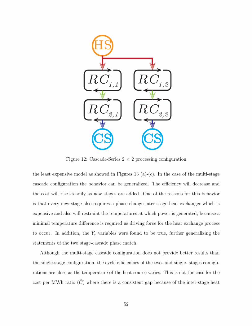
RC
HS
CSCS
1,2
RC2,2
RC1,1
RC2,1
Figure 12: Cascade-Series 2 × 2 processing configuration
the least expensive model as showed in Figures 13 (a)-(c). In the case of the multi-stage
cascade configuration the behavior can be generalized. The efficiency will decrease and
the cost will rise steadily as new stages are added. One of the reasons for this behavior
is that every new stage also requires a phase change inter-stage heat exchanger which is
expensive and also will restraint the temperatures at which power is generated, because a
minimal temperature difference is required as driving force for the heat exchange process
to occur. In addition, the Ys variables were found to be true, further generalizing the
statements of the two stage-cascade phase match.
Although the multi-stage cascade configuration does not provide better results than
the single-stage configuration, the cycle efficiencies of the two- and single- stages configu-
rations are close as the temperature of the heat source varies. This is not the case for the
cost per MWh ratio (C) where there is a consistent gap because of the inter-stage heat
52

exchanger as previously discussed. The results of the series multi-stage configuration are
more regular since there is little variation as new stages are added in consistence with
the two-stage configuration results. The absorbed heat in each stage is a proportional
fraction of what the single-stage model does. Therefore, when a new stage is added the
costs will be balanced and the cost ratio (C) will remain almost constant. In comparison
with the single-stage, the multi-stage series configuration is less efficient no matter the
number of stages, except for the 90 C two-stage configuration case. This, in combination
with the cascade results, suggest that the multi-stage configurations feature almost no
improvement when the temperature is raised over the single-stage. Finally, the 2 × 2
hybrid configuration features almost the same level of thermodynamic efficiency (η) with
respect to the tree-stage cascade model, but with lower electricity annual cost. However,
the results are not better than the two-stage configuration or the single-stage process.
In summary, the multi-stage configurations were only effective at only one temper-
ature. For the kind of organic fluids considered in this work, the single-stage model
will be always the best choice. Although, the availability and size of equipment of the
multi-stage configuration could possibly be an advantage over the single-stage process,
especially when the series configuration is adopted, since the efficiency and cost are kept
almost constant with stage inclusion. It also could be possible that in a dynamic environ-
ment, some configuration would be more well-behaved than the others in terms of process
operability. In the case of the cascade configuration, the main difficulty is the inter-stage
heat exchanger, which could be substituted by a direct contact heat transfer scheme, and
thus overcoming the limitations of efficiency and cost. However, from a computational
point of view, this will require a larger number of variables and equations since more
regions of variable composition must be included.
53

*
(a) η at 363.15 K (90 C)
*
(b) η at 373.15 K (100 C)
*
(c) η at 383.15 K (110 C)
Figure 13: Efficiency η for the configurations at different temperatures. Single stage,Sp-e (Series-Cascade efficiency), Sp-c (Series-Cascade C), Cascade-e (efficiency), Series-e(efficiency), Cascade-C (C), Series-C (C)
54

*
(a) C at 363.15 K (90 C)
*
(b) C at 373.15 K (100 C)
*
(c) C at 383.15 K (110 C)
Figure 14: Annual Cost for the configurations at different temperatures.
55

5 Conclusions
The heat available at low temperature is a potential source for power through the Rankine
cycle. But because of the difficulties implied by low temperature, the Rankine cycle must
be modified. The modifications currently proposed by various authors have dealt with the
working fluid selection, and the Rankine cycle optimization. In this work we deploy two
multiple coupled cycles: the series and cascade configurations. If all the cycle variables are
selected in a systematic way, an improvement of performance is expected. Additionally, if
we consider the working fluid of a mixture of defined components as a degree of freedom, it
is possible that the simultaneous determination of these variables generates an even better
improvement. All the considerations involving the multi-stage Rankine cycle design with
mixtures as working fluids, were implemented into an algebraic model that was solved for
optimality with deterministic approaches. For this, two objective functions were analyzed
individually. The implementation of the cascade model was found to require complex
constraints that can be formulated through generalized disjunctive programming (GDP).
The results show that the multistage approaches are only useful for the two-stage case
at low temperature in terms of the efficiency. But, they are intrinsically more expensive
than the single stage Rankine cycle because of the necessity of more equipment for every
single situation. As temperature progresses, none of the multistage configurations is better
than the single stage. For the cascade cycle, the phase matching logical variables show
that in the case of cascade configurations, the best match is always at the two phase
region. But the existence of this intermediate heat transfer stage results in the more
costly configuration because this requires an expensive heat exchanger, and as stages are
added the cost raises steadily. The series configuration, although marginally less efficient
than the single stage, turned out to keep almost the same objectives as stages are added.
Although the results favored the single stage approach as the temperature increases, it can
be worth to verify if multistage Rankine cycles display better operability, controllability
56

features and to examine how uncertainty affects the results presented in this work. Both
topics will be addressed in future work.
57

Nomenclature
Indexes
i, j ∈ I component of the mixture
s ∈ STG stage
SL last stage
k,m, n ∈M functional group
f ∈ F phase
L liquid
V vapor
π ∈ Π equilibrium point
p ∈ L pressure level
o ∈ O subcool point
o ∈ O superheat point
O nonequilibrium points
58

Condensed notation of constraints and variables
Zs EOS equations
Gs activity coefficients equations
Bs equilibrium and property equations
ϕs operation constraints
Cs cost equations
U1
s single stage constraints
UC
s multi-stage cascade constraints
US
s multi-stage series constraints
tLs (liq) multi-stage cascade LP liquid match
tLs (2P) multi-stage cascade LP 2-phase match
tUs (vap) multi-stage cascade HP liquid match
tUs (2P) multi-stage cascade HP 2-phase match
P s Pressure
T s Temperatures
zs Compositions
X Operating variables(e.g. molar flows, HX areas, fugacity coefficients, etc)
Variables
Symbol Description Units
(Aie′)s Heat exchanger intermediate two-phase m2
(Ail′)s Heat exchanger intermediate liquid m2
(Aiv′)s Heat exchanger intermediate vapor m2(ALe′)s
Heat exchanger area two-phase LP m2(ALl′)s
Heat exchanger area liquid LP m2(ALv′)s
Heat exchanger area vapor LP m2
AHe′ Heat exchanger area two-phase HP m2
59

AHl′ Heat exchanger area liquid HP m2
AHv′ Heat exchanger area vapor HP m2
aSsop Mixture EOS var n-eq. dimensionless
aS′sop Mix. EOS variable temp. derivative n-eq. bar cm3 kmol−1 K−1
aRisp EOS variable Ref. dimensionless
aR′isp EOS variable temp. derivative ref. K−1
aS′isop EOS variable temp. derivative n-eq. K−1
auis EOS variable dimensionless
aupis EOS variable pure K−1
a′isp EOS variable temp. derivative K−1
aus EOS variable dimensionless
a′sp Mix. EOS variable temp. derivative bar cm3 kmol−1 K−1
ˆaups Mixture EOS variable bar cm3 kmol−1 K−1
(BCP )s Updated bare pump cost $
(BCT )s Updated bare turbine cost $
(BiCX)s Updated bare heat exchanger cost intermediate $
BHCX Update bare heat exchanger cost HP $(BLCX
)s
Update bare heat exchanger cost HP $
bsπp Mixture EOS variable cm3 kmol−1
bRisp EOS variable Ref. dimensionless
bSsop Mix. EOS variable n-eq. dimensionless
bus EOS variable dimensionless
CWWyr Cost of cooling water $
C Cost per annual MWh $ MWh−1(DHRid
)isp
Ideal gas enthalpy change ref. kJ/Hu(DhRlv
)isp
Vaporization enthalpy change kJ/Hu
60

(fRT )isp EOS temp. Funct. at ref. temp. dimensionless
EG Electricity generated 1 yr basis MWh
(fR′T )isp EOS variable temp. Derivative ref. K−1
(fST )isop EOS temp. Funct. at nonequilibrium temp. dimensionless
(fT )isπp EOS temperature function dimensionless
(f ′T )isp EOS variable temp. Derivative K−1
(fS′T )isop EOS variable temp. Derivative n-eq. K−1
Kisπp Equilibrium ratio dimensionless(LMTDH
e′
)s
Log mean temperature difference HP 2-phase K(LMTDH
l′
)s
Log mean temperature difference HP liquid K(LMTDH
v′
)s
Log mean temperature difference HP vapor K(LMTDi
e′
)s
Log mean temperature difference inter. H-ex. 2-phase K(LMTDi
l′
)s
Log mean temperature difference inter. H-ex. liquid K(LMTDi
v′
)s
Log mean temperature difference inter. H-ex. vapor K(LMTDL
e′
)s
Log mean temperature difference LP 2-phase K(LMTDL
l′
)s
Log mean temperature difference LP liquid K(LMTDL
v′
)s
Log mean temperature difference LP vapor K
dHHSsπ Enthalpy point of heat source kJ/Hu
DHiuis Ideal enthalpy change kJ/Hu
fTuis EOS temperature function dimensionless
fTupis EOS T function pure T. der K −1
FC Overall Updated cost of equipment $
GS′sop Gibbs excess temp. der. bar cm3 kmol−1 K−1
GSsop Gibbs excess dimensionless n-eq. dimensionless
G′sp Gibbs excess temp. der. bar cm3 kmol−1 K−1
GsπV p Gibbs excess dimensionless dimensionless
61

Hpsπp Enthalpy point at eq. kJ/Hu(HR)sp
Residual enthalpy dimensionless
HRRFisp Ref. residual enthalpy dimensionless
HRus Residual enthalpy dimensionless
(HR)sop Residual enthalpy n-eq. dimensionless
HSsop Vapor enthalpy n-eq. kJ/Hu
hSsop Liquid enthalpy n-eq. kJ/Hu
hsp Liquid enthalpy kJ/Hu
Hsp Vapor enthalpy kJ/Hu
Hupsp Vapor enthalpy kJ/Hu
lGPiksπp Activity contribution mix. Pure dimensionless
ns Mole flow of working fluid kmol s−1
nCs Mole flow of heat sink kmol s−1
P satisπp Saturation Pressure bar
Psp Pressure at level s bar
PWWyr Cost of water (Heat source) $ m-3
Qsp Heat kJ/Hu(sTRid
)isp
Ideal gas entropy change ref. kJ K−1 /Su
(SR)sop Residual entropy n-eq. dimensionless(SR)sp
Residual entropy dimensionless(SR)sp
Ref. residual entropy dimensionless
SSsop Liquid entropy kJ K−1 /Su
sSsop Liquid entropy n-eq. kJ K−1 /Su
ssp Liquid entropy kJ K−1 /Su
Ssp Liquid entropy kJ K−1 /Su
(SP )s Pump design value gpm × psi
62

(ST )s Turbine design value hp
Tks Intermediate temperature of stage K
tLs Low pressure match K
TRFisp Reference temperature K
TSsop Temperature at nonequilibrium K
tUs High pressure match K
TwCsπ Heat sink temperature at equilibrium K
TwHsπ Heat source temperature at equilibrium K
VLs Vapor fraction low pressure K
VC overall cost of utilities $
Tsπp Temperature at equilibrium K
xisfπp equilibrium composition dimensionless
Xmsπfp functional group mole fraction dimensionless
Y liqs Boolean variable HP liquid match true,false
Y 2Ps Boolean variable HP two phase match true,false
Y vaps Boolean variable LP vapor match true,false
Y 2Ps Boolean variable LP two phase match true,false
(WP )s Work (positive) pump kJ/Hu
(WT )s Work (positive) turbine kJ/Hu
Zsatisπp Saturation Comp. Fact. dimensionless
ZRisp Ref. Compressibility Factor dimensionless
Zus Compressibility factor dimensionless
Zsπp Mix. Compressibility factor dimensionless
ZSsop Mix. Compressibility factor n-eq. dimensionless
zis Global composition dimensionless
ηI Efficiency by the 1st law of Thermodynamics dimensionless
63

αisπp Mixture EOS variable dimensionless
αsπp Mixture EOS variable dimensionless
αisπp Molar part. EOS variable dimensionless
αsπp Mixture EOS variable dimensionless
βsπp Mixture EOS variable dimensionless
βsatisπp EOS var at saturation dimensionless(∆H id
)isp
Ideal gas enthalpy change kJ/Hu
(∆Hs)isop Ideal gas enthalpy change n-eq. kJ/Hu
∆Hlisp Liquid enthalpy change kJ/Hu
∆HlSisop Liquid enthalpy change n-eq. kJ/Hu
∆Hes Enthalpy change at stage kJ/Hu(∆Sid
)isp
Ideal gas entropy change kJ K−1 /Su
(∆Ss)isop Ideal gas entropy change n-eq. kJ K−1 /Su
∆Slisp Liquid entropy change kJ K−1 /Su
∆SlSisop Liquid entropy change n-eq. kJ K−1 /Su
Ψmksπp UNIFAC interaction var. dimensionless
ψu Vapor fraction high pressure dimensionless
θmsπfp functional group area fraction dimensionless
ln γisπfp Activity coefficient natural logarithm dimensionless
ln γCisπfp Activity coefficient combinatorial dimensionless
ln γRisπfp Activity coefficient residual dimensionless
ln Γksπfp Activity contribution mix. dimensionless
(ln Φsat)isπp Saturation fugacity coefficient dimensionless(ln Φ
)isπp
Mixture fugacity coefficient dimensionless
Parameters
64

Symbol Description Units
A1 PSRK parameter (-0.64666) dimensionless
amn UNIFAC binary interaction parameter K
bi EOS parameter (0.008446RgTci/Pci) cm3 kmol−1
cω,i Acentric function (0.48 + 1.574ωi − 0.176ω2i ) dimensionless
C0T Cost factor turbine $
C0X Heat exchanger cost coefficient $
C0P Cost coefficient pump $
C1,i − C7,i Vapor pressure parameters see Eq. 39 & 40
cpx1i Ideal gas heat capacity parameter kJ K−3
cpx2i Ideal gas heat capacity parameter kJ K−2
cpx3i Ideal gas heat capacity parameter kJ K−1
cpl1i Liquid heat capacity parameter kJ K−3
cpl2i Liquid heat capacity parameter kJ K−2
cpl3i Liquid heat capacity parameter kJ K−1
CEPCI CE plant cost index (579.8) dimensionless
CSF0 Cost of water adjustment parameter $ m−3
CSFyr Cost of water adjustment parameter for year yr $ m−3
DHFi Formation enthalpy change kJ kmol−1
DGFi Formation Gibbs energy change kJ kmol−1 K−1
DHHT Heat source overall enthalpy change (∫ TwmxTwmn
CpHdT ) kJ /Hu
F0P Update factor pump $
F0T Update factor turbine $
F0X Update factor HX $
Hu Enthalpy scaling factor (104) dimensionless
lj UNIFAC parameters dimensionless
65

nH Heat source mole flow kmol s−1
Pci Critical pressure bar
Qk UNIFAC parameters dimensionless
qi UNIFAC parameters dimensionless
Rg Gas constant bar cm3 kmol−1 K−1
Rk UNIFAC parameters dimensionless
ri UNIFAC parameters dimensionless
Su Entropy factor (103) dimensionless
S0T Cost factor turbine hp
S0X Heat exchanger cost coefficient m2
S0P Cos coefficient pump gpm × psi
Twmn Heat source minimum temperature K
Twmx Heat source maximum temperature K
TwCmn Heat sink minimum temperature K
TwCmx Heat sink maximum temperature K
Tci Critical temperature K
Tbri Normal boiling temperature K
TPim UNIFAC pure molecule fraction area dimensionless
Ul′ Overall heat transfer coef. liquid kW K−1 m−1
Ue′ Overall heat transfer coef. two phase kW K−1 m−1
Uv′ Overall heat transfer coef. vapor kW K−1 m−1
U il′ Overall heat transfer coef. intermediate liquid kW K−1 m−1
U ie′ Overall heat transfer coef. intermediate two phase kW K−1 m−1
U iv′ Overall heat transfer coef. intermediate vapor kW K−1 m−1
yr year 1,2,...,yrL
XPim UNIFAC mole fraction pure mole. dimensionless
66

αP Cost coefficient pump dimensionless
αT Cost factor turbine dimensionless
αX Heat exchanger cost coefficient dimensionless
∆hBLVi Normal boiling point enthalpy change kJ kmol−1
νim UNIFAC group frequency on mole. i dimensionless
ηMP Mechanical efficiency pump dimensionless
ηMT Mechanical efficiency turbine dimensionless
ηT Turbine efficiency dimensionless
ηP Pump efficiency dimensionless
ψπ Vapor fraction dimensionless
67

References
[1] Badr, O.; Probert, S.; O’Callaghan, P. Selecting a working fluid for a Rankine-cycle
engine. Appl. Energ. 21(1):1–42, 1985.
[2] Larjola, J. Electricity from industrial waste heat using high-speed organic Rankine
cycle (ORC). Int. J. Prod. Econ. 41(1):227–235, 1995.
[3] Linke, P.; Papadopoulos, A. I.; Seferlis, P. Systematic Methods for Working Fluid
Selection and the Design, Integration and Control of Organic Rankine Cycles-A Re-
view. Energies 8(6):4755–4801, 2015.
[4] Mavrou, P.; Papadopoulos, A. I.; Seferlis, P.; Linke, P.; Voutetakis, S. Selection of
working fluid mixtures for flexible Organic Rankine Cycles under operating variability
through a systematic nonlinear sensitivity analysis approach. Appl. Therm. Eng.
2015.
[5] Braimakis, K.; Preißinger, M.; Bruggemann, D.; Karellas, S.; Panopoulos, K. Low
grade waste heat recovery with subcritical and supercritical Organic Rankine Cycle
based on natural refrigerants and their binary mixtures. Energy 2015.
[6] Lampe, M.; Stavrou, M.; Bucker, H.; Gross, J.; Bardow, A. Simultaneous optimiza-
tion of working fluid and process for organic Rankine cycles using PC-SAFT. Ind.
Eng. Chem. Res. 53(21):8821–8830, 2014.
[7] Lecompte, S.; Huisseune, H.; van den Broek, M.; Vanslambrouck, B.; De Paepe, M.
Review of organic Rankine cycle (ORC) architectures for waste heat recovery. Renew.
Sust. Energ. Rev. 47:448–461, 2015.
[8] Molina-Thierry, D. P.; Flores-Tlacuahuac, A. Simultaneous optimal design of organic
mixtures and Rankine cycles for low-temperature energy recovery. Ind. Eng. Chem.
Res. 54(13):3367–3383, 2015.
68

[9] Kosmadakis, G.; Manolakos, D.; Kyritsis, S.; Papadakis, G. Economic assessment
of a two-stage solar organic Rankine cycle for reverse osmosis desalination. Renew.
Energ. 34(6):1579–1586, 2009.
[10] Morisaki, T.; Ikegami, Y. Maximum power of a multistage Rankine cycle in low-grade
thermal energy conversion. Appl. Therm. Eng. 69(1):78–85, 2014.
[11] Yun, E.; Kim, D.; Yoon, S. Y.; Kim, K. C. Experimental investigation of an organic
Rankine cycle with multiple expanders used in parallel. Appl. Energ. 145:246–254,
2015.
[12] Li, T.; Zhang, Z.; Lu, J.; Yang, J.; Hu, Y. Two-stage evaporation strategy to improve
system performance for organic Rankine cycle. Appl. Energ. 150:323–334, 2015.
[13] Stijepovic, M. Z.; Papadopoulos, A. I.; Linke, P.; Grujic, A. S.; Seferlis, P. An exergy
composite curves approach for the design of optimum multi-pressure organic Rankine
cycle processes. Energy 69:285–298, 2014.
[14] Smith, J.; Van Ness, H.; Abbott, M. Chemical engineering thermodynamics.
McGraw-Hill, NY 2001.
[15] Holderbaum, T.; Gmehling, J. PSRK: A group contribution equation of state based
on UNIFAC. Fluid Phase Equilib. 70(2):251–265, 1991.
[16] Kamath, R. S.; Biegler, L. T.; Grossmann, I. E. An equation-oriented approach for
handling thermodynamics based on cubic equation of state in process optimization.
Comput. Chem. Eng. 34(12):2085–2096, 2010.
[17] Fredenslund, A. Vapor-liquid equilibria using UNIFAC: a group-contribution method.
Elsevier, 2012.
69

[18] Kleiber, M. An extension to the UNIFAC group assignment for prediction of
vapor-liquid equilibria of mixtures containing refrigerants. ”Fluid Phase Equilib.
107(2):161–188, 1995.
[19] Dahl, S.; Michelsen, M. L. High-pressure vapor-liquid equilibrium with a UNIFAC-
based equation of state. AIChE J. 36(12):1829–1836, 1990.
[20] Poling, B. E.; Prausnitz, J. M.; John Paul, O.; Reid, R. C. The properties of gases
and liquids, volume 5. McGraw-Hill New York, 2001.
[21] Henley, E. J.; Seader, J. Equilibrium-Stage Separation Operations in Chemical En-
gineering. John Wiley, 1981.
[22] Rowley, R.; Wilding, W.; Oscarson, J.; Yang, Y.; Zundel, N.; Daubert, T.; Danner,
R. DIPPR Data Compilation of Pure Chemical Properties. Des. Inst. Phys. Prop.
2006.
[23] Aspen Technology Inc. Aspen Plus v8.4 2014. URL https://www.aspentech.com/
products/engineering/aspen-plus/.
[24] Grossmann, I. E. Review of nonlinear mixed-integer and disjunctive programming
techniques. Optimization and Engineering 3(3):227–252, 2002.
[25] Trespalacios, F.; Grossmann, I. E. Review of Mixed-Integer Nonlinear and General-
ized Disjunctive Programming Methods. Chem. Ing. Tech. 86(7):991–1012, 2014.
[26] Kreith, F. The CRC handbook of thermal engineering. Springer Science & Business
Media, 2000.
[27] Awad, M. M. Fouling of heat transfer surfaces. INTECH Open Access Publisher,
2011.
70

[28] Biegler, L. T.; Grossmann, I. E.; Westerberg, A. W. Systematic methods for chemical
process design. Prentice Hall, Old Tappan, NJ (United States), 1997.
[29] Access Intelligence. Plant Cost Index. Chemical engineering [Online] 2015. URL
http://www.chemengonline.com/pci-home.
[30] Ulrich, G. D.; Vasudevan, P. T. How to estimate utility costs. Chemical Engineering
113(4):66–69, 2006.
[31] Brooke, A.; Kendrick, D.; Meeraus, A.; Raman, R. GAMS: A User’s Guide. GAMS
Development Corporation: Washington, DC, 1981.
[32] Drud, A. S. CONOPT- a large-scale GRG code. ORSA J. Comput. 6(2):207–216,
1994.
[33] Vecchietti, A.; Grossmann, I. E. LOGMIP: a disjunctive 0–1 non-linear optimizer for
process system models. Computers & Chemical Engineering 23(4):555–565, 1999.
71