w

SINGLE LINK FLEXIBLE

BEAM TESTBED PROJECT

by

Declan Hughes

u

Rensselaer Polytechnic Institute

Electrical, Computer, and Systems Engineering Department

Troy, New York 12180-3590

m July 1992

m CIRSSE REPORT #120

https://ntrs.nasa.gov/search.jsp?R=19930012118 2018-08-31T02:57:43+00:00Z

I

i

i

[]

mnil

i

n

i

H

i1

i

U

ii

i

i

n

m

i

i

CONTENTS

m

w

m

r_u

m

u

m

m

M

=-

LIST OF TABLES ................................. v

LIST OF FIGURES ................................ vi

ACKNOWLEDGMENTS ............................. viii

ABSTRACT .................................... ix

INTRODUCTION ................................. x

1. Hardware .................................... 1

1.1 Overview .................................. 1

1.2 Selecting the Flexible Beam ....................... 1

1.3 Actuator .................................. 3

1.4 Sensors ................................... 5

1.4.1 Hub Angle ............................. 5

1.4.2 Beam Strain ............................ 6

1.5 Computer ................................. 6

1.5.1 Real Time Computer ....................... 6

1.5.2 Development Host Computer .................. 8

1.5.3 Computer to Signal Interface .................. 8

2. Software ..................................... 10

2.1 Software Overview ............................ 10

2.2 Program Description ........................... 12

2.3 Resetting Signal Offsets ......................... 13

3. Beam Modeling ................................. 15

3.1 Beam Analytical Modeling ........................ 15

3.1.1 Linear Differential Equations .................. 15

3.1.2 Normal Mode Form ........................ 16

3.1.3 Finite State Space Normal Mode Approximation ........ 20

3.2 Hub Actuator ............................... 20

3.3 Hub Angle Sensor ............................. 21

ii

i

m[]

:7

|

|

[]

[]

]

i

i

i

i

i

_

i

i

i

i

i

=

I

i

w

= ,

m

n

w

3.3.1 Angle to Voltage Conversion ................... 22

3.4 Beam Strain Sensors ............................ 22

3.4.1 Strain Gage Geometry ...................... 23

3.4.2 Curvature-Strain Linear Relationship .............. 26

3.4.3 Curvature-Strain Non-linear Relationship ............ 27

3.4.4 Strain to Voltage Conversion ................... 28

3.4.5 Strain Gage Signal Conditioner ................. 28

3.5 Computer Input and Output ....................... 29

3.6 Complete Testbed State Space Model .................. 30

3.7 Model Structural Features ........................ 31

3.8 Model Identification ........................... 33

3.8.1 Oscillation Frequencies ...................... 34

3.8.2 Damping coei_cients ....................... 34

3.8.3 Modal Gains ........................... 35

3.8.4 Identification Improvements ................... 35

4. Control Design ................................. 37

4.1 Overview .................................. 37

4.2 Positive Realness ............................. 39

4.3 The Passivity Theorem .......................... 41

4.4 Hub Angle PD Compensator ....................... 42

4.4.1 Closed Loop Stability ....................... 42

4.4.2 Pdgid Body Mode Plant ..................... 43

4.4.3 Root Locus Design ........................ 44

4.5 Synthesized Positive Real Output Controller (static feedback) .... 48

4.5.1 Selecting C,_a (decoupled version) ............... 51

4.5.2 Selecting C3p_ (coupled version) ................. 52

4.6 State Estimation ............................. 52

4.6.1 Full State Observers with Uncompensated Modes Effects . . . 54

4.6.2 Reduced Order (Luenberger) Observer with Uncompensated

Modes Effects ........................... 56

5. Simulation and Experimental Results ..................... 58

5.1 Simulation Results with Ideal Observer ................. 58

,°,

111

__o

w

J

5.2 Closed Loop Observers Effects ...................... 61

5.3 Experimental Results with Reduced Order Luenberger Observer . . . 63

CONCLUSIONS 68

LITERATURE CITED • - • . ..... ...... . .............. 69

APPENDICES _ =.......... 70

A. Beam and Actuator Physical Parameters ................... 70

=,_

mm

I

m

mm

m

m

7÷ =.=

mim

|

mm

mm

,,m

mm

mm

I

mm

M

iv

mm

mm

mm

7

w

LIST OF TABLES

Table I.i

Table 3.1

Table 4.1

Table 4.2

Table 4.3

Table A.1

Table A.2

Table A.3

Table A.4

Candidate Beam Materials .................... 3

Beam Normal Mode Parameters ................. 19

PD Compensator Gains ..................... 46

Compensator Pole Parameters .................. 47

Lyapunov Equation relative Weights .............. 51

Aluminum Beam Material Parameters ............. 70

Beam Derived Parameters .................... 70

Motor Parameters ......................... 71

Hub Derived Parameters ..................... 71

E

r

V

I

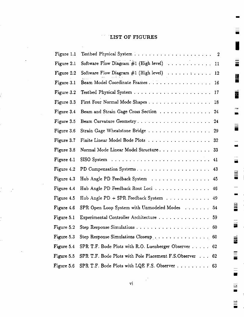
LiST OF FIGURES

Figure i.i

Figure 2.1

Figure 2.2

Figure 3.1

Figure 3.2

Figure 3.3

Figure 3.4

Figure 3.5

Figure 3.6

Figure 3.7

Figure 3.8

Figure 4.1

Figure 4.2

Figure 4.3

Figure 4.4

Figure 4.5

Figure 4.6

Testbed Physical System 2

Software Flow Diagram-#1 (High level) ............ 11

Software Flow Diagram #1 (High level) ...... . ..... 12

Beam Model Coordinate Frames - 16

Testbed Physical System ..................... 17

First Four Normal Mode Shapes ................. 18

Beam and Strain Gage Cross Section .............. 24

Beam Curvature Geometry .................... 24

Strain Gage Wheatstone Bridge ................. 29

Finite Linear Model Bode Plots ................. 32

Normal Mode Linear Model Structure .............. 33

SISO System ........................... 41

PD Compensation Systems .................... 43

Hub Angle PD Feedback System ................ 45

Hub Angle PD Feedback Root Loci ............... 46

Hub Angle PD + SPR Feedback System ............ 49

SPR Open Loop System with Unmodeled Modes ....... 54

Figure 5.1

Figure 5.2

Figure 5.3

Figure 5.4

Figure 5.5

Figure 5.6

Experimental Controller Architecture .............. 59

Step Response Simulations .................... 60

Step Response Simulations Closeup ............... 60

SPR T.F. Bode Plots with R.O. Luenberger Observer ..... 62

SPR T.F. Bode Plots with Pole Placement F.S.Observer . . . 62

SPR T.F. Bode Plots with LQE F.S. Observer ......... 63

vi

mm

!i

I

m

I

m

mm

Im

B

u

m

I

J z

m

II

mm

I

mm

=_Ill

w

w

Figure 5.7

Figure 5.8

Figure 5.9

Experimental Step Response with Different Observers ..... 64

Synthesized SPR Output Comparison .............. 65

Step Response Experimental Results .............. 65

Figure 5.10 Step Response Experimental Results Closeup ......... 66

Figure 5.11 Experimental Bode Plots ..................... 67

m

m

i

L_

i

vii

ACKNOWLEDGMENTS

I would like to thank Dr. John Wen for his continued patience, support, and ideas

which are a major part of this thesis. I would also like to thank Judy Bloomingdale,

Denise Elwell, Betty Lawson and Diane Brauner for their help in getting things done

and Deepak Sood, Michael Repko, Steven Murphy and Chris Seaman for kindly

showing me the ropes at CIRSSE.

D

im

N

mm

I

B

mm

r,m

M

=

==

I

M

m

==

mD

U

,,o

Vlll

m

mm

i

m

I

\

ABSTRACT

m

: = .

m

This thesis describes the single link flexible beam testbed at the CLAMS laboratory

in terms of its hardware, software and linear model and presents two controllers, each

including a hub angle PD feedback compensator and one augmented by a second

static gain full state feedback loop, based upon a synthesized strictly positive real

(SPR) output, that increases specific flexible mode pole damping ratios w.r.t the

PD only case and hence reduces unwanted residual oscillation effects. Restricting

full state feedback gains so as to produce a SPR open loop transfer function ensures

that the associated compensator has an infinite gain margin and a phase margin of

at least [-90, 90] degrees. Both experimental and simulation data are evaluated

in order to compare some different observer performances when applied to the real

testbed and to the linear model when uncompensated flexible modes are included.

m

2=

w

i

ix

INTRODUCTION

This thesis is organized into five chapters describing the hardware, software, mod-

eling, control design and test results for the single link flexible manipulator system

at the CLAMS laboratory. The testbed is designed so as to enable the study of the

identification and control of a realflexlble system and the concept is similar to that

of the earlier work done by Cannon and Schmitz (see e.g., [3]).

Chapter onedetails the hardware which is centered on an aluminum beam

(a plate), driven by a motor at one end while the other end is free, which was

designed to exhibit low frequency poorly damped flexible modes. The real time

c0ntrolling microprocessor iSi20 Mhz Inmos Transputer mounted on a motherboard

attached to a VME backplane : analog to digital and digital to analog converter

' "cards mounted on the same backplane provide external signal interfaces. Currently

a hub angle sensor and beam strain sensors are used while two tip displacement

sensors are being installed, namely a light sensor and an induction sensor.

The second chapter describes the main software functions which implement

linear and non-linear controllers and run on two transputers : three controllers

are designed in this thesis and each is characterized by a fixed interval discrete time

linear observer and compensator pair. Also, beam parameter identification is carried

out with the same software. Reference trajectories and controller parameters are

loaded from Matlab data files before each experiment and afterwards the resulting

data is stored in a similar fashion for later analysis. Before each experiment the

D/A and A/D converter DC offsets may be loaded from another Matlab data file

or updated via a short (about 25 seconds) test routine.

Chapter three outlines the linear modeling of the beam, from the governing

pair of linearized partial differential equations to a finite normal mode approximation

in state space form and the computation of the output sensor matrix for the hub

=

BI

=

I

il

ml

mU

=

m

l

i

m

I

mR

=u

M

i

I

I

I

x

I

g

u

L .

B

w

angle potentiometer and beam strain gages. This linear model is characterized by a

collection of second order transfer functions (the beam modes) driven by a common

input torque and each sensor can be viewed as a linear combination of the associated

states. The rigid body mode contains a stable real pole and a pole at the origin whilst

each of the others have a very poorly damped but stable complex pole pair with

a unique oscillation frequency (these are called the flexible modes). The complete

transfer function is thus the linear combination of the individual modal transfer

functions each of which dominates close to its center frequency. A brief description

of the identification process is also given : direct modal parameter identification is

.. used.

The fourth chapter describes two full state compensators designed to improve

the beam tip displacement response and each requires an observer to provide the

state estimate. The first controller designed is a hub angle PD compensator which

is found to give very good results in terms of tip displacement step response time,

..... . overshoot and residual oscillations. The design method used is simple : initially ig-

nore the flexible modes and select those PD compensators which move the two rigid

body mode poles such that the second order closed loop system is, say, critically

damped. Then restore the flexible mode dynamics and select a single PD compen-

sator from the previous set that also increases the flexible mode pole damping ratios

with particular emphasis placed on the lowest frequency mode.

PD compensation is a form of static gain full state feedback that has the

advantage of an infinite gain margin in the ideal case (i.e. perfect modeling) and

this will remain true for the actual plant closed so long as the torque to estimated hub

angle velocity transfer function remains strictly positive real (SPR) as is guaranteed

by the Passivity Theorem. However observer, sensor and other errors will make the

actual system more fragile.

The second controller designed is constructed by adding another static gain

xi

I

feedback loop designed so as to further increase the damping ratios of the flexible

modes. For this loop the time domain definition of strict positive realness is em-

ployed to synthesize a SPR output from the state estimate of the PD compensated

plant that emphasizes selected flexible modes. By restricting the class of feedback

gains in this fashion we can guarantee that static negative feedback applied to this

SPR SISO system will have an infinite gain margin and a phase margin of at least

[-90, 90] (again in the ideal case).

The actual gains are selected through trial and error however there is a strong

correlation between the improvement in individual flexible mode pole damping ratios

and corresponding terms in the synthesized SPR output matrix parameterization.

Two such SPR outputs are selected, one with a modal transformation applied to

the PD compensated system so as to explicitly decouple the flexible modes, and the

other with the original coupled PD compensated system.

Several closed loop observer designs are selected, namely a LQE full state ob-

:_ .... server, a pole placement full state observer and a reduced order Luenberger observer.

In the fifth and final chapter some simulations and experimental results are

examined in order to evaluate the performance of the controller/observer combina-

tions in step response tests. The distorting effects of the observers in conjunction

with unmodeled beam modes on the synthesized SPR transfer function is exam-

ined through simulations and the observer which most faithfully reconstructs this

transfer function (and performs well when applied to the true plant) is selected. Ex-

perimental bode plots are also examined since they give a good indication of flexible

mode pole damping ratios.

mR

w

B

[]

g

B

mm

I

mm

m

U

I

l

U

I

xii

m

i

i

m

CHAPTER 1

Hardware

m

,4 o: • •°,vr

1.1 Overview

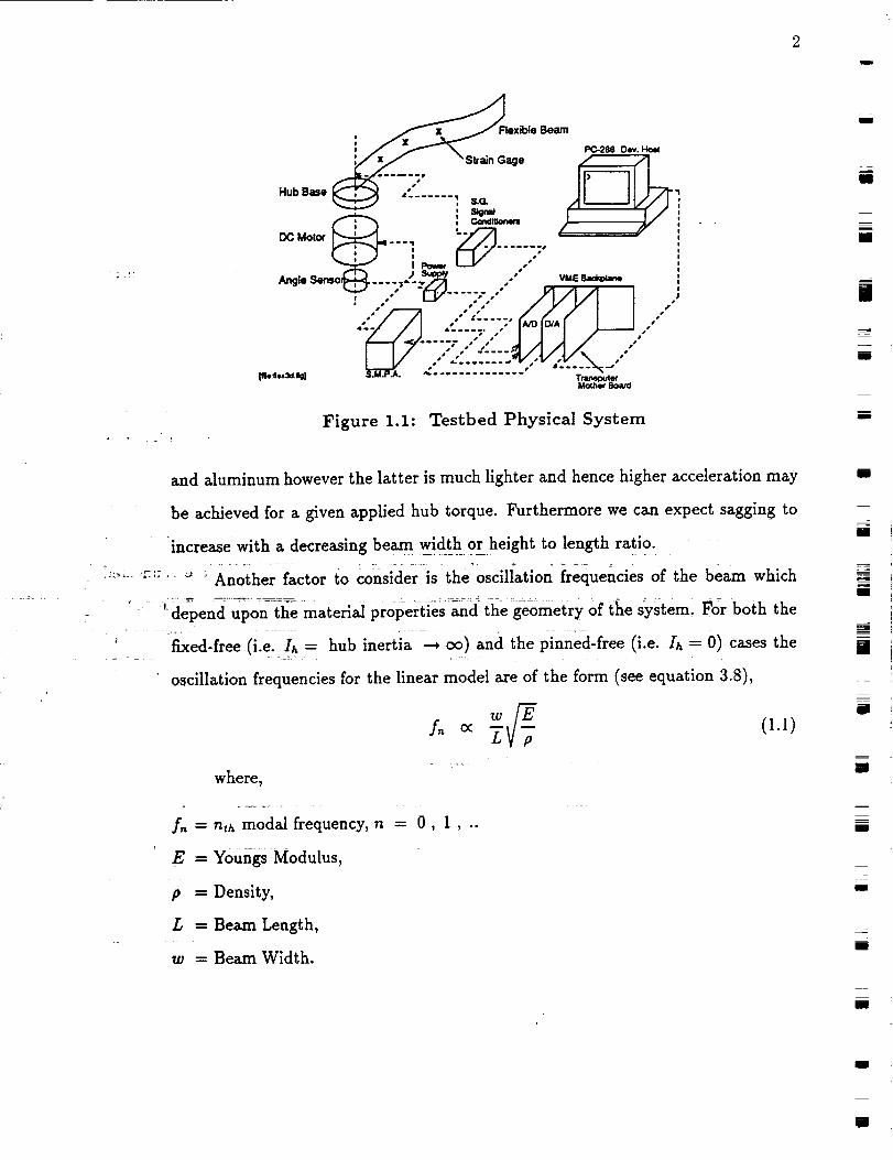
Figure 1.1 is an outline of the physical single flexible link testbed the central

component being the flexible beam itself which is chosen to provide readily measur-

able flexibility in the horizontal plane that is independent of gravity (ideally). This

is driven by a DC motor at one end about a vertical axis in order to excite the flexible

modes, and the other end is free. The motor is energized by a power amplifier which

itself is controlled by a single voltage signal; the power amplifier-motor combination

provides an approximately linear voltage to beam hub torque relationship. The hub

angle is converted to a voltage signal by a potentiometer while the beam strains

at specific locations are likewise converted by strain gages. The realtime computer

is a networked set of four Inmos Transputer micro-processors which are connected

to a PC-AT host for software development and user interface. These Transputers

also connect to a VME signal bus on which resides the digital to analog (D/A) and

analog to digital (A/D) circuit cards providing the motor drive (computer output)

and sensor (computer input) signal interfaces.

1.2 Selecting the Flexible Beam

A problem with a single flexible plate (i.e., a thin beam) is that the unsup-

ported end can sag due to the effect of gravity when the beam is flexed and this is a

source of nonlinear behavior and an unwanted complication. To minimize this effect

a high Youngs modulus to density ratio is desired in order to maximize strength

and minimize weight and mainly for this reason aluminum was selected as the beam

material over steel, brass or plastic (see table 1.1); this ratio is similar for both steel

, /.,/_"x/x_Flexible Beam

: / _ _2. o.,.Ho,

',/x/;';" _' SI1ain Gage f ,/]

DC Motor i _ i_ "'f / I

i U/ .....:'"," "tr-_..) ....... " 1/I /I /1 I

, . t--V ," ," / I/ I/ I I ,'0 wo s ,, f

• o o • •../----A .., ..,,'=d/ I I or °

0o S o • _' Bj •

Figure 1.1: Testbed Physical System

and aluminum however the latter is much lighter and hence higher acceleration may

be achieved for a given applied hub torque. Furthermore we can expect sagging to

" increase with a decreasing beam width or height to length ratio.

" .... _;:-' :" = Another factor to consider is the oscillation frequencies of the beam which

" _depend_ ..............upon the material' properties _d the geometry of t]ae system. For both the

; fixed-free (i.e. h = hub inertia _ oo) and the pinned-free (i.e. In = 0) cases the

oscillation frequencies for the linear model are of the form (see equation 3.8),

w E

where,

f, = nth modal frequency, n = 0, 1 , ..

E = Youngs Modulus,

p = Density,

/., = Beam Length,

(i.I)

w = Beam Width.

m

N

i

|

m

u

u

m

m

[]

g

m

m

HI

m

i

i

3b .

=

mTable 1.1: Candidate Beam Materials

Material

units

Aluminum, Alloy 6061.

Steel, Type 302.

Brass, CA 230.

Plexiglas, typical values.

Density

Kg/m 3

2.713e3

8.028e3

8.748e3

1.18 e3

Youngs Mod.

Kg/m 2

6.895e10

1.957ell

1.172ell

2.969e09

_/E/p

5.041e3

4.937e3

3.660e3

1.586e3

m

r

r

m

w

When the hub inertia lies somewhere between the two extremes given above

the equation for f,_ becomes more complex however the values for f,, will fall between

those of the fixed-free and pinned-free cases.

In order to minimize the computer speed requirement low oscillation frequen-

cies are desired and hence we wish to minimize the width to length ratio and min-

imize the Youngs modulus to density ratio, however this will have the effect of

increasing sagging at the tip and hence a compromise is required.

A beam length of approximately one meter was chosen to provide a relatively

large structure that will not be significantly affected by multiple sensors (e.g. strain

gages, hub angle sensor, position light sensors) and to minimize the effects of hub

shaft friction. Several beams of aluminum, steel and plastic were examined with a

height of ten centimeters approximately and a width such that the fourth frequency

was close to 50Hz and the aluminum beam was selected as it sagged the least and

had a low weight.

1.3 Actuator

w

A DC motor and switch mode power amplifier were selected to drive the beam

as this combination provides a good degree of inherent open loop linearity at a

reasonable cost and is a common method of actuating robot joints. The motor is a

PMI Disc DC motor which contains no rotor iron other than the central shaft (the

4m

coils are compressed into a flat disc) and this provides four main benefits,

1. no inter-coil iron implies no cogging torque, a common unwanted non-linearity

in other DC motor types,

2. the rotor mass is concentrated near the shaft axis and hence has a low inertia

Which yields high acceleration; in the complete setup the hub mounting is the

main hub inertial component,

3. the small rotor coils have a low inductance value which increases the ampli-

fier/motor bandwidth,

4. low coil inductance eliminates commutation brush sparking which reduces mo-

tor generated electrical noise.

The main disadvantage of this particular motor is the shaft friction torque due

to brush/coil contact and the use of solid bearings.

A switch mode power amplifier, as its name implies, operates as a switch

to alternatively apply full motor rotor coil voltage in one direction and then the

other at a high frequency (20Khz nominal). This is obviously a highly nonlinear

process however the switching process is controlled so that the motor current is

nearly linearly proportional to the input voltage signal over smaller bandwidth (e.g.

1Khz) which is more than sufficient for our purposes. The only reasons for the

switching operation are amplifier design considerations eg. power efficiency and

component cost.

The motor/amplifier combination provides a low pass filter voltage to torque

transfer function and the dominant pole location is determined by the rotor circuit

resistance and inductance,

I/LR

r the dominant pole time constant,

(1.2)

m

I

m

U

mI

i

zI

mi

I

m

m

mI

i

m

mI

D

I

I

R =

rotor circuit inductance,

rotor circuit resistance.

5

i

m

w

i •

and is estimated to be 2rnsec approximately which means a 500 Hz bandwidth.

While the low rotor inductance is desirable'in order to maximize this band-

width it has the unfortunate effect of increasing the motor rms current which de-

termines the heat dissipated. A small inductor was added into the rotor circuit to

contain this effect doubling the overall inductance (this is included in the 500Hz

bandwidth estimation).

1.4 Sensors

1.4.1 Hub Angle

• A potentiometer was chosen for sensing the hub angle because it is cheap

and because the interface circuitry is very simple (assuming an A/D converter is

avaiIible). However other options exist which can provide better resolution and

accuracy and less noise disturbance e.g., an optical angular encoder or a resolver

and one of these will eventually replace the potentiometer.

Being an analog sensor the potentiometer has infinite resolution but its accu-

racy is limited by circuit and contact noise and any non-linearity in the resistive

material; the former affects relative accuracy while the latter reduces absolute ac-

curacy. Furthermore, since the A/D converters have a 12 bit word length and

the potentiometer translates +/- 180 degrees into to the A/D full scale voltage

of +] - 10V the actual hub angle resolution is limited to 0.0879 degrees approxi-

mately. When the beam is at rest this corresponds to a tip displacement resolution

of approximately 1.68mm.

-m

6m

high quality matched resistors.

1.5 Computer

1.4.2 Beam Strain

Thin film strain gages are used to sense beam longitudinal strain at four points

along the beam and the particular strain gages selected have the following features,

1. a small size to provide a local measurement,

2. a temperature drift coefficient to offset aluminum heat expansion,

3. capable of measuring large repeated strains.

In each case the strain gages are mounted in pairs on either side of the beam

so that the resistance of one increases when the beam bends while the resistance

of the other decreases; each pair forms part of a wheatstone bridge circuit and this

arrangement provides good immunity to unwanted side effects such as temperature

dependancies or contact potentials: the rest of the bridge circuit is comprised of two

1.5.1 Real Time Computer

The real time computer is a network of four Inmos Transputers (see figure/

2.1, only two are in use at present) which may be readily expanded in the future

as proccessing requirements dictate. The Transputer is a single chip microprocessor

which is availible in several formats and we use the T800-20 model which runs

at 20Mhz and is rated at 20 MIPS and 2.8 Mflops peak instruction rates. Each

Transputer contains the following,

1. 32 bit CPU

2. 64 bit FPU

3. 4 Kbytes of fast static RAM

4. four 20 Mbit/sec bidirectional serial links

I

m

mmm

m

I

g

B

l

[]

m

m

I

l

mmm

[]

i

I

I

u

m

[]

7

5. 32 bit data and memory busesand a DRAM controller

m

b.

m

The Transputers are specifically designed for external parallel operation using

the high speed serial links for interconnections and these links also connect the

transputers to the host development computer and the signal interface data bus.

The transputers are also designed to facilitate multi-tasking (each separate

program is called a process and high speed switching is achieved between separate

processes on the same Transputer) and this constitutes a second form of parallelism.

Separate processes communicate with each other through channels, not shared mem-

ory, and if the processes lie on different Transputers then these channels are mapped

to the physical hardware links before runtime. In this way the code may be re-

distributed across different nets by simply defining a new mapping operation and

therefore the processes need not be rewritten. Thus there are two distinct networks,

the real hardware form and the desired software form. Note that while any number

of software channels (memory permitting) may exist between processes running on

the same Transputer, this is not the case for inter-Transputer communication as

each Transputer has exactly four serial links.

A third form of parallelism exists since the transputer allows the CPU, FPU

and link interfaces to operate in parallel which further improves the computers

performance if software is written to take advantage of this feature.

The high level parallel language Occam was developed to make optimal use

of the Transputers hardware features and thus experimental control and data in-

put/output algorithms are written in this language. The code used was originally

written in MicroSoft Quick C (almost ANSI C compatible) for an PC-AT386 based

system and now an Inmos ANSI C compiler is used for non-speed critical sections

while the rest has been converted to Occam.

8I

1.5.2 Development Host Computer

The user interface to the Transputers is provided by a PC-AT286 micro com-

puter and when developing the software the Occam or ANSI C compilers and linkers

axe downloaded to the transputers along with the source code which then performs

the compilation, linking and network configuring. At runtime the Transputers are

reset-karl then the executable code is downloaded and booted.

m

z

m

|

Zm

1.5.3 Computer to Signal Interface

1.5.3.1 Interface Card Bus

A VMEbus was selected to interface the Transputers to the A/D and D/A

cards because of its large data bandwidth and the the wide variety of compatible

circuit cards that exist and also because it is the bus used by an adjacent laboratory

(the CIRSSE Dual Robot Arm Testbed). This bus supports 8, 16 and 32 bit data

words at a maximum speed 40M/-/'z and the backplane is mounted along with the

circuit power supply in a Eurocard rack.

z

B

m

i

I

= 1.5,3.2 A/D Converters

The A/D card selected is a XVME-566 made by XYCOM and features 32

single ended, or 16 differential, input channels with 12 bit resolution and 12 bit

accuracy. One channel may be sampled at a time (the conversion time is 10/_sec)

with a maximum sample throughput rate of lOOKhz and any number of channels

up to the maximum may be sampled in any sequence and the results stored in on

board RAM.

In the current configuration single ended bipolar voltage input (+/- 10V) is

used, the programmable gain is set to unity and the data ram is memory mapped

to one of the Transputer microprocessors via the VMEbus so that each sample is

accessed by a direct memory read command.

m

I

I

M

m

m

m

i

l

[]

i

i

i

9

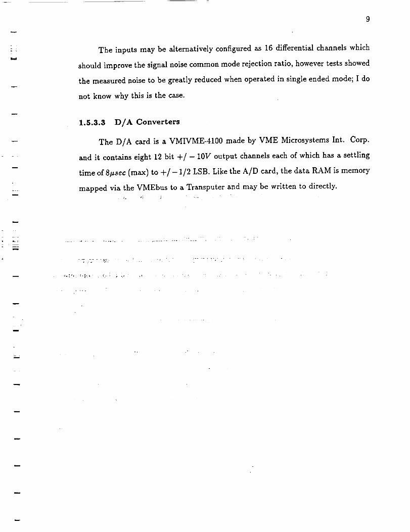
--! The inputs may be alternatively configured as 16 differential channels which

should improve the signal noise common mode rejection ratio, however tests showed

the measured noise to be greatly reduced when operated in single ended mode; I do

not know why this is the case.

=

!

i

1.5.3,3 D/A Converters

The D/A card is a VMIVME-4100 made by VME Microsystems Int. Corp.

and it contains eight 12 bit +/- 10V output channels each of which has a settling

time of 8_t_ec (max) to +/- 1/2 LSB. Like the A/D card, the data RAM is memory

mapped via the VMEbus to a Transputer and may be written to directly.

= _

m

CHAPTER 2

Software

R

m

2.1 Software Overview

The original computer program was written in Microsoft Quick C (almost

ANSI C compatible) to run on a PC-386; C was chosen for several reasons, the

main ones being, .......

1. it has a relatively fast compiled code execution,

2. it is the most commonly used language amongst the students

3. and faculty working in the laboratory

4. it is a flexible language capable of implementing complex data structures.

The PC-386 has now been replaced by a set of four micro-processors, the Inmos

Transputers, interconnected by high speed serial data links and a host computer (a

PC-286) for file handling and the user interface in order to greatly increase compu-

tation power and to facilitate further expansion if so desired; the Transputers and

their links constitute the computer hardware network (see figure 2.1).

Optimum performance is obtained if software is written in the language Occam

which was developed by Inmos for the Transputers and therefore the speed critical

control and data I/O interface algorithms were converted to two separate processes

using the Inmos Parallel Occam compiler while the rest of the original program (i.e..

the user interface and file handling section) was recast as a single process using

the Inmos Parallel ANSI C compiler. The processes communicate with each other

and the host through asynchronous data channels; the processes and their channel

configuration constitute the software network and this is distributed amongst the

hardware network as shown in figure 2.1.

10

1m

i

I

E

!

i

m!i

i

i

I

m

[]

D

l

t

D

I

I

i1

m

m

m

m

m

L ,

m

w

w

m

n

7,

i. wo__.w_.___lm ..... w-_ I

! I

' T800-20 #0 ' T800-20 #3PC LO; _ I ', r

[......: "i- ad ..... .........i

VME ', j.._

Bus _ ' ' ----T800-20 #I T800-20 #2

!

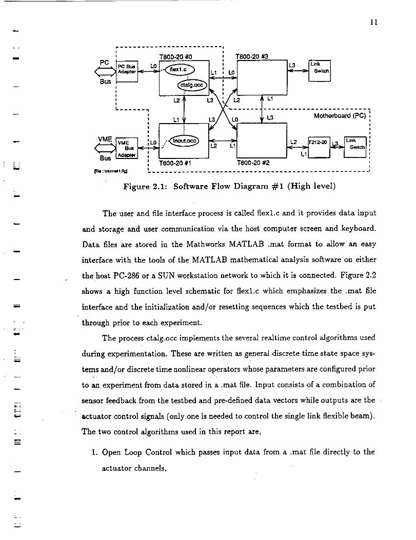
Figure 2.1: Software Flow Diagram #1 (High level)

The user and file interface process is called flexl.c and it provides data input

and storage and user communication via the host computer screen and keyboard.

Data files are stored in the Mathworks MATLAB .mat format to allow an easy

interface with the tools of the MATLAB mathematical analysis software on either

the host PC-286 or a SUN workstation network to which it is connected. Figure 2.2

shows a high function level schematic for flexl.c which emphasizes the .mat file

interface and the initialization and/or resetting sequences which the testbed is put

through prior to each experiment.

The process ctalg.occ implements the several realtime control algorithms used

during experimentation. These are written as general discrete time state space sys-

tems and/or discrete time nonlinear operators whose parameters are configured prior

to an experiment from data stored in a .mat file. Input consists of a combination of

sensor feedback from the testbed and pre-defined data vectors while outputs are the

actuator control signals (only one is needed to control the single link flexible beam).

The two control algorithms used in this report are,

1. Open Loop Control which passes input data from a .mat file directly to the

actuator channels,

L

w

J

12m

_ Roed In Control

1

._ Reed in Comp4msatorMmtrlces

1

I =

A/D and I_A OffoeW

'"1- l

I Run Sek_-_d _ Fletumthe BmlmControl AI11a,llhm to the Origin

I[mo:caow_,Joj

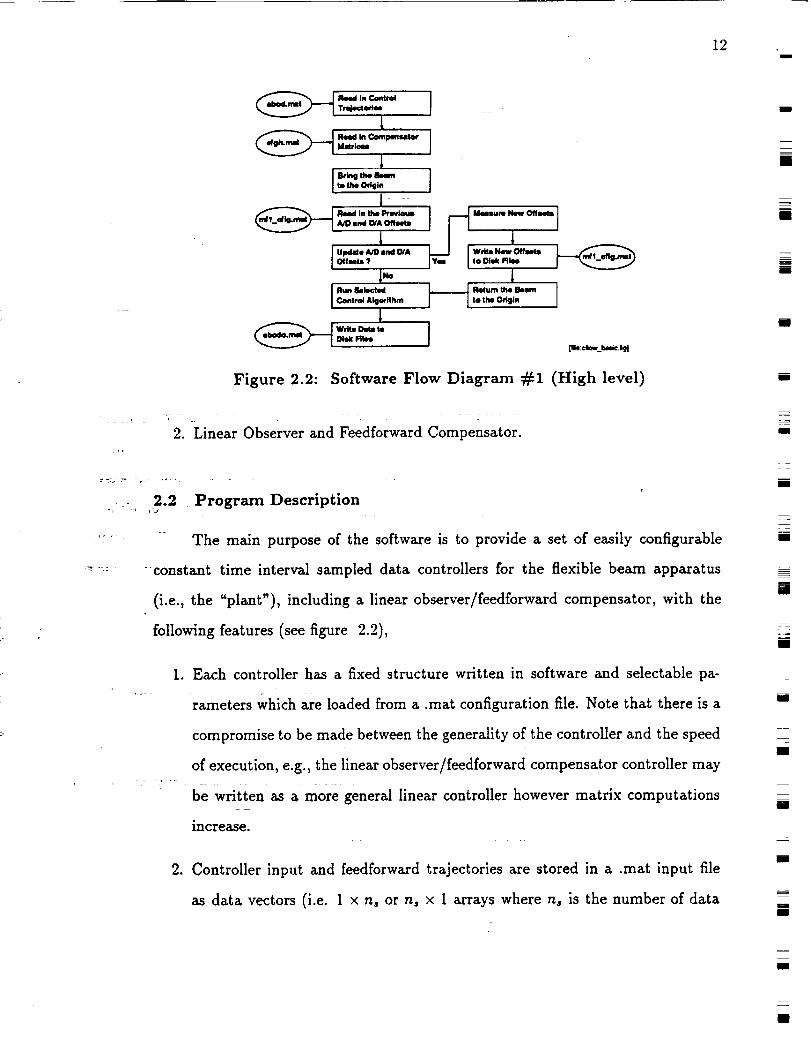
Figure 2.2: Software Flow Diagram #1 (High level)

2. Linear Observer and Feedforward Compensator.

.... 2.2 Program Description

_, -=:

The main purpose of the software is to provide a set of easily configurable

constant time interval sampled data controllers for the flexible beam apparatus

(i.e., the "plant"), including a linear observer/feedforward compensator, with the

following features (see figure 2.2),

1. Each controller has a fixed structure written in software and setectable pa-

rameters which are loaded from a .mat configuration file. Note that there is a

compromise to be made between the generality of the controller and the speed

of execution, e.g., the linear observer/feedforward compensator controller may

be written as a more general linear controller however matrix computations

increase.

2. Controller input and feedforward trajectories are stored in a .mat input file

as data vectors (i.e. 1 × n, or n, × 1 arrays where ns is the number of data

m

m

m

01

m

mm

M

m

m

mm

m

zm

I

m

mm

z

U

mmm

mm

m

mm

mI

n

w

m

M

w

13

samples taken during the experiment),

3. Controller output (i.e., plant input) and plant feedback to the controller vec-

tors are stored in a .mat output file after the experiment.

4. Plant input and output signal steady state offsets may be automatically mea-

sured prior to each experiment, stored in a .mat file, and compensated for

during the experiment.

5. Both the sampling time interval ts and the number of samples taken during

an experiment are specified in the input file.

2.3 Resetting Signal Offsets

Each analog component of the testbed hardware is subject to nominal signal

changes between experiments due to temperature induced drifts, aging of compo-

nents, and distortions caused by the experiments themselves (e.g., a large strain on

the flexible beam can slightly bend it so that the strain gage steady state values mea-

surably change). In order to minimize the effects of such errors the software includes

an option to measures these offsets prior to the experiment and the I/O procedure

then automatically compensates (by subtracting from A/D values and adding to

D/A values). Furthermore the new offsets are stored in a .mat file (mfl_cfig.mat)

and are used during subsequent experiments until they are measured again; in prac-

tise the offsets are usually updated prior to each experiment.

Strain gage signal offsets are measured by averaging a series of readings taken

over five seconds while the beam is at rest (i.e., the input torque is at zero) while

the potentiometer offset is always set to zero for experiments where the absolute

zero angle is unimportant.

The offset related to the motor amplifier circuit is more problematic due to

the effect of hub shaft friction. In the absence of friction the unique amplitude of

n

14i

the signal applied to the power amplifier would equal the offset when the motor

is at rest and hence be easily measured. However in actuality the beam will come

to rest if the applied motor field torque is less than the friction dynamic threshold

and remain there as long as the static threshold in not exceeded and hence zero

applied torque condition is not readily detected. One solution is to apply a dither

signal directly to the motor amplifier and add a proportional negative feedback loop;

assuming a su_ciently large dither signal and convergence of the operating point to

a periodic cycle the amplifier circuit offset will correspond to the average applied

torque signal. In practice a lOHz signal is applied and after a pause of 5 seconds

the average over 5 seconds of the torque signal is calculated.

J

R

I

m

i

iI

I

m

m

D

m

m

mm

==m

I

mm

B

m

=

m

M

mI

= ,

u

w

m

m

CHAPTER 3

Beam Modeling

3.1 Beam Analytical Modeling

3.1.1 Linear Differential Equations

The essential model components of the testbed are the beam itself driven by

a torque at the hub, and the effective hub inertia. Figure 3.1 shows the coordinate

frames and geometric notation used in the following equations. The correspond-

ing non-linear beam model was derived in [1] using Hamilton's Principle with the

following initial assumptions,

1. Hooke's Linear Stress-Strain Law holds.

2. The beam elongation is negligible.

w

3. The beam deformation is small.

4. The hub and bending velocities are small.

and a set of linearized partial differential equations was subsequently obtained,

62vEI._4 + p_- _ =0 (3.1)

":-_::-_ " - "1"- Iu¢ + EI_v"(O,t) = 0 (3.2)

=.,

with the boundary conditions

_(0,t)

E

Pa:

= 0,1; v'(0,t) = 0, v"(o,t) =

= beam material Youngs Modulus

= the input motor torque,

= the beam mass per unit length,

1.5

o, ,/"(L,t) = O,

f

16I

I

I

1I

tIIII

hub(

yo

X,e beam--'_w(x) X "_ :

sjP_ooO.O _-° °'_Ip

iI II ....:_'- I 1 __ X o

] [m.:mcxJt_._]__ _

Figure 3.1: Beam Model Coordinate Frames

Ih = hub inertia,

L = the beam length,

v = w+z¢,

¢ = rigid body mode angle,

Oh = the hub angle,

w(x) = beam displacement at x meters along the nominal axis.

3.1.2 Normal Mode Form

An eigen-analysis of these equations is performed in order to establish the

infinite set of modal frequencies {wi} at which the beam exhibits resonance (damping

is not included in the model at this stage) and corresponding mode shapes {¢_(x)},

including one rigid body mode (w0 = 0, ¢0(x) = a straight line) where,

Bi

Di

-- A, sin(k,z) + B, sinh(k,z) + C_ cos(k,z) + D,, cosh(k_z)

= cch+*sh+lci-, ch + c sh

-- -C,

(3.3)

(3.4)

(3.5)

(3.6)

I

ii

I!

I

II

m

i

I

i

I

N

I

I

I

iI

m=m

I

I

I

I

I

I

I

I

17

m

= =

._h_ r----__- .................... , SMPA -_--_-_-'-.........

dachanO , .......

rfchan_l)- ControIFL'13me _ k_ Potenliorneter __AJgodbhm _ S.G.s + W.Sridges

I

,_U_r_t_.._.._J_ v. 13___,._L.__..jw';Conditioner

• Vt

!

Computer + D/A & A/D Hardware

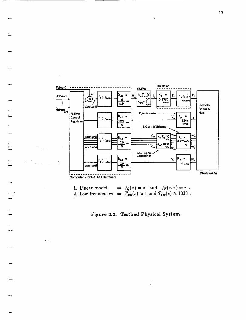
1. Linear model =_ fo(z) = z and fF(r, ÷) = r .

2. Low frequencies _ T,,,,(s) _ 1 and T,,(s) _ 1333.

Rexible

Beam &

Hub

Figure 3.2: Testbed Physical System

18g

0

-2

A

EL

RJRidBo( y Mode Shape

0 0.5 !

X '<m._

Flexible Mode/02

2

0

-2

0

! i

i0.5 1

x ,_rn>

A

M

Flexible Mode #1

2

0

-2

0

........................... i ............................

i i

O.5

Flexible Mode #3

2 ......................... : ...................... _ .....

• I i

0 0.5 1

X .,_n.>'

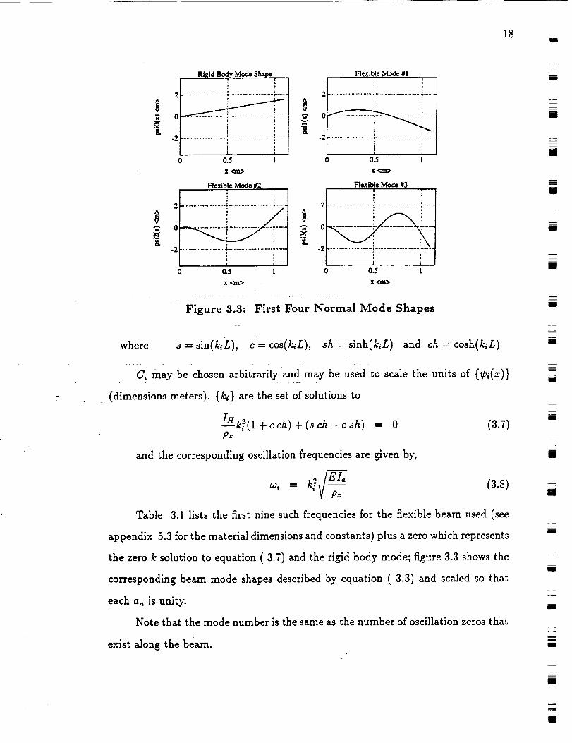
Figure 3.3: First Four Normal Mode Shapes

where s = sin(k,L), c = cos(k,L), sh = sinh(kiL) and ch = cosh(k,L)

Ci may be chosen arbitrarily and may be used to scale the units of {¢i(z)}

(dimensions meters). {k_} are the set of solutions to

/Hk/3(1 +cch)+(sch-csh) = 0 (3.7)P_

and the corresponding oscillation frequencies are given by,

(3.8)= "

Table 3.1 lists the first nine such frequencies for the flexible beam used (see

appendix 5.3 for the material dimensions and constants) plus a zero which represents

the zero k solution to equation (3.7) and the rigid body mode; figure 3.3 shows the

corresponding beam mode shapes described by equation (3.3) and scaled so that

each a,_ is unity.

Note that the mode number is the same as the number of oscillation zeros that

exist along the beam.

mm

u

[]

I

I

z

m

mm

n

I

mm

mI

mm

I

I

N

, =

I

g

u

19

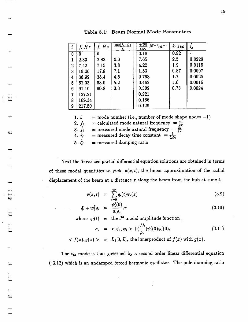
Table 3.1: Beam Normal Mode Parameters

u

w

0

1

2

3

4

5

6

7

8

9

fi Hz fi Hz '°°(I-'-/i) _ N-'m -1 _'i secn fi a, lpz

0 0 3.19 0.92

2.83 2.83 10.0 7.65 2.5

7.42 7.15 13.8 4.22 1.9

19.06 17.8 17.1 1.53 0.87

36.99 35.4 14.5 0.768 1.7

61.03 58.0 15.2 0.462 1.6

91.10 90.8 10.3 0.309 0.73

127.21 0.221

169.34 0.166

217.50 0.129

1. i

2. fi3.]i4.4

¢,

0.0229

0.0115

0.0097

0.0025

0.0016

0.0024

= mode number (i.e., number of mode shape nodes -1)

= calculated mode natural frequency = _21r

= measured mode natural frequency = _-27r

= measured decay time constant -

= measured damping ratio

e..._

told

Next the linearized partial differential equation solutions are obtained in terms

of these modal quantities to yield v(x, t), the linear approximation of the radial

displacement of the beam at a distance x along the beam from the hub at time t,

OO

v(x,t) = __, qi(t)¢i(x) (3.9)

2qi + wi qi = • (3.10)

aip_

where qi(t) = the i th modal amplitude function,

< ¢i,¢i > +(_h)¢_(0)_b_(0), (3.11)ai

< f(x),g(z) > = L2[0, L], the innerproduct of f(x) with g(z),

The i,hmode is thus governed by a second order linear differential equation

(3.12) which is an undamped forced harmonic oscillator. The pole damping ratio

w

r_

20I

(_i) for each flexible mode is now estimated experimentally and inserted to produce,

_li + 2(iwi4i-4" oJ_qi -- _(0) r (3.12)

aipr

8.1.3 Finite State Space Normal Mode Approximation

The A and B matrices of a finite state space representation n modes cam now

be easily derived from equation (3.12) if we truncate the model after the n th mode

= A,,,x + B._r where, (3.13)

Af!tl "-- , Br =

0 1 0 0 ... 0 0

0 -do 0 0 ... 0 0

0 0 0 1 ... 0 0

0 0 -wt 2 -dz ... 0 0

: : : : - :

0 0 0 0 ... 0 i

o o o o ...

• ],qo qo ql qz .-- q_-I q_-t

0

apz

0

npz

0

• apz

(3.14)

z = (3.15)

Currently used are a hub angle sensor (a potentiometer) and four strain gages

mounted along the beam and in each case the signals produced cam be approximated

by a linear combination of the states z(i) to produce the output C matrix, and the

D matrix is null and the corresponding Sensor velocities are obtained by shifting the

appropriate C matrix rows one place to the right in order to meet the q',_ states.

=

3.2 Hub Actuator

With reference to figure 3.2 the switch mode power amplifier and DC motor

dynamics may be approximated by the following linear transfer function relation-

ship,

r(s) = k,.k_,,,,T_,_(s)V_(s) (3.16)

g

m

m

m

g

m

g

m

m

m

I

m

U

I

m

m

21

where To,_(8) = r_m (3.17)

and k_ - I,,,(s) ' the motor torque constant. (3.18)

Here r_,,, is the dominant time constant of the power amplifier and DC motor

field winding circuit, T_,,,(s) is the associated low pass transfer function due to

resistance and inductance (see chapter 1) and k_ is the low frequency switch mode

power amplifie/DC motor voltage to motor circuit current (I,_) gain. Since r_,_

and is estimated to be 2 milliseconds approximately; it is neglected (i.e., assumed

infinite) for the purposes of this report as the highest modal frequency considered

is 58Hz, and hence equation (3.17) may be approximated by

r(8) = k_k_V,_(s). (3.19)

w

k.-

w

m

L _

3.3 Hub Angle Sensor

Equation (3.13) describes the torque to modal state transfer function and we

_. _-_- - _ *--" .....now relate the modal state to the hub angle ¢ ; the truncated form of equation (3.9)

implies

rL !

¢ = v'(O,t) = E,=o q_(t)¢i(0) (3.20)

where ¢_(0) is the derivative of the i th mode shape at the origin (i.e., the hub

shaft) and is found by differentiating equation (3.3) . Equation 3.20 can be recast

in state space form as,

¢ = C,x (3.21)

= 0 0 ... 0] (3.22)

Note that C, can be related to B_. (see equation (3.14) as follows:

65 "- B_P_ (3.23)

w

22M

where P_ is a diagonal strictly positive definite matrix and since the only

system pole that is not exponentially stable (i.e., the rigid body mode pole at the

origin) is decoupled from the hub velocity output the Positive Realness Theorem

guarantees that the torque to hub angle transfer function is strictly positive real,

(see chapter 4).

3.3.1 Angle to Voltage Conversion

A single turn potentiometer is used to convert the hub angle ¢ to a voltage

signal: with reference to figure 3.2

V_ (3.24)V_ = ¢.kp and kp = 2-'_

where V, is the potentiometer supply voltage, and kp is the conversion constant.

3.4 Beam Strain Sensors

The longitudinal strain at a specific point on the beam surface is closely related

to the curvature w"(x, t) of the beam at that point and we can relate the latter to

the modal states in truncated form as follows,

w"(=,t)=v"(=,t)i

= _ q,.,(t)'C,_'(z) (3.25)i=1

where ¢_'(x) are given by equation 3.3 and therefore in state space form,

w"(=,t) = c.(=)=

c.(=) = [oo _i'(=)o ... ¢"(=)o ].

(3.26)

(3.27)

Note that Co(X) may be calculated explicitly and is found to be

Ls 1i.I)=¢o(=) = v_( T + p: (3.28)

and hence _,_'(z) is zero for all x.

M

mmlira

m

mm

m

m

88

m

mm

m

U

lira

I

mm

I

m

I

mm

m

m

U

_ 23

b

_:--

3.4.1 Strain Gage Geometry

The strain gages are mounted in pairs opposite to each other on either side of

the beam so that together they can measure the extent of bending at a particular

distance along the beam, half way up the side. (see figure 1.1). Only one strain

gage is strictly necessary at each point of interest, however considerable noise and

disturbance immunity is achieved by using them in pairs as one arm of a Wheatstone

bridge configuration (see figure 3.6). In fact four strain gages completing the bridge

circuit are even better, two mounted on each side of the beam close together, but it

is not clear that the performance improvement over two is significant and worth the

extra cost and construction. Figure 3.4 shows a cross section of the beam with a pair

of strain gages on either side (looking down from above the beam). The important

dimensions are,

and

db_tiw_

d_

dglue

dtilm

d,/2

= the width of the beam,

= strain gage substrate thickness,

= estimated glue thickness,

= thickness of strain gage film,

= db,_,,,/2 + dgt,te "4" d,,,b + dfit,,/2 (3.29)

7.938x10 -4+5x10 -r = 8.438 x 10 -4 (3.30)

=

is the distance between the beam neutral axis and the center of the strain gage

film half the effective beam width with respect to the strain gages.

A strain gage, of the type used, is a pattern of resistive material whose resis-

tance increases when stretched and when the beam bends in a clockwise direction

(cw)(looking down from above) the cw+ strain gage is elongated and so its length

undergoes positive strain (hence the name cw+), while at the same time, the cw-

strain gage is forced to contract, implying negative strain. The strain gages are very

linear devices over a wide range of strains and the altered resistances increase V,g

24J

S.g. film s.g. proteclive coaling I y

s g substtale I / _

"" \ L " c___L° "" z/

...........................___.

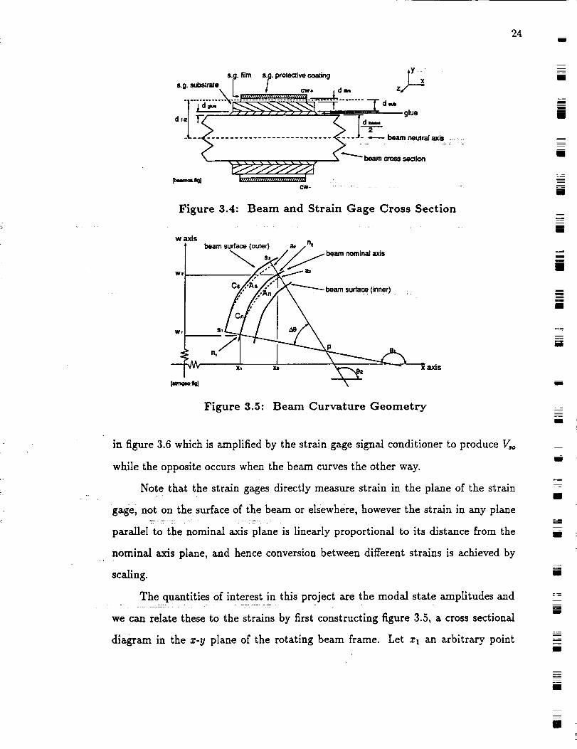
Figure 3.4: Beam and Strain Gage Cross Section

w axis

Wl

W,

beam surface (outer) az / r_

n/

X_ Xl

X axis

Figure 3.5: Beam Curvature Geometry

in figure 3.6 which is amplified by the strain gage signal conditioner to produce _o

while the opposite occurs when the beam curves the other way.

Note that the strain gages directly measure strain in the plane of the strain

gage, not on the surface of the beam or elsewhere, however the strain in any plane

parallel to the nominal axis plane is linearly proportional to its distance from the

nominal axis plane, and hence conversion between different strains is achieved by

scaling.

The quantities of interest in this project are the modal state amplitudes and

we can relate these to the strains by first constructing figure 3.5, a cross sectional

diagram in the z-y plane of the rotating beam frame. Let z_ an arbitrary point

m

nmm

m

i

mI

m

i

I

B

I

I

I

=

m

Z

g

m

_=

_ 25

along the beam neutral axis when at rest (ie. the z axis) with wl w(xl)) as the

nominal axis displacement associated with the linear model; nl - (:rl,wl). Also

choose a:2 such that

=.=:.

w

x2 -- x1"f Ax,

It is assumed that Ax is chosen sufficiently small such that the segment of the

n.a. C,_, ( -= [ nl , n2 ] ), is continuously convex w.r.t, a particular side of the

beam. Let A,_ be the corresponding nominal axis curve section, length l,, (i.e., A,, is

a circular arc centered at p and connecting nl to the transverse plane line through

n2). At nl and n2 extend the beam transverse lines until they meet at some point

p and let R_ be the length of [ ni , p ] ; 8, is the angle between the x axis and the

transverse lines. The transverse plane and outer surface intersections are labeled sl

and s2 and the connecting beam curve is called C, with a corresponding nominal

axis curve section A,.

Let

9t,

AO

[¢.n -_

I'#C" "-

L_$ ----

0,- 90 degrees, i= 1,2 ( then w_ = tan(St,)) (3.31)

02 - 01 = 0t2 - On, (3.32)

length(C,,), l,,,_= length(A,,) (3.33)

length(C,) = l_ + Ale, (3.34)

length(A,) = Is,, + AI_, (3.35)

J

i

where Aim and AI,,, are the n.a. curve and arc length extensions due to strain

deformation respectively.

26 m

3.4.2 Curvature-Strain Linear Relationship

The following limits are assumed

lim --C'* = 1,ax-o A,

lim l_,,Ax_o/a---_ = 1,

lim_ = 1,Ax-,O AI¢_

lim C, = 1,ax-o A,

lim--L" = 1,Ax--O Las

Azlira = cos(0t,).

AZ-..*0

(3.36)

(3.37)

(3.38)

Now

and therefore

_3_,._:, i -- :_,;:_._SO _ 'tO 1 -"

R, AO = I_,,,

4e_r_

::,. AO = AI,,,2

(R1 + -_-_-_)A# = la. + Al_,, (3.39)

(3.40)

sin(f,,o)/ (cos(o. )cos(o._))

lim (w_-w'2) = lim sin(AO)A_...o Ax a_-o cos(0,)cos(0,_)_z

1 AO

- lim -- =cost(On) a_ o Az

1 lim AI_----A

-- _ cos3(Otl)a=-o le.,2

1 lim Alc...._,

- _ cos3(0,,) at.--.o Io2

1 lim Al.o

cos_(O,,) a_-o /xx

1 lim AI_= _ cosa(Otx) a=--.o I_

2

el

= _ cos3(O.)2

(3.41)

(3.42)

(3.43)

(3.44)

(3.45)

where et is the beam convex surface engineering strain (and a convex surface

implies that e, is positive). Lastly

el = lim _ (3.46)le,--0 [ca

A _ ,, d_.= cosZ(8.) ) (3.47)and hence e,, = el = w,(_

" (dl_2) (3.48)W 1 _ esl

for small deflection angles On where e, is the strain experienced by the corre-

sponding strain gage, (the strain in the opposite strain gage is equal to -e,). The

m

mm

BI

mu

i

=I

mm

m

mJ

I

=_mm

i

mD

I

Bm

mm

mm

B

27

i

term _ is due to the fact that the active part of the strain gages are raised from

the beam surface and hence the true distance from the center of the beam is larger

than halve the actual beam width.

m

=

h .b

3.4.3 Curvature-Strain Non-linear Relationship

Equation 3.47 is nonlinear and may be expanded as follows

w_ = tan(St1) =_ cos2(0tl)(w'l) 2 = (1 -cos2(0t,)) (3.49)

cos2(Ot,) = (1 + (w_)2) -' (3.50)

cos3(O.)= (1+ (3.51)dtrtam it

wl (3.52)= (1+

Assuming that (w_) _ << 1, a binomial expansion implies that

col = -_W_'(1 - 3/2(w_) 2 + 0((w'1)4)) (3.53)

and since w_ may be expressed in terms of the modal states

w'l(t) = v'(zl,t) - ¢(t) = _ qi(t)[¢_(z_) - ¢_(0)] (3.54)i=0

equation (3.48) may be modified to included a power series approximation to

the nonlinear relationship up to any desired order :

,, _ _ 3/2(w_) 21w_ _ ( )(1 + O((w_)4) )e,_. (3.55)

For the discrete model a previous estimate of the plant may be used in order

to calculate w_ and this then be subsequently used in equation (3.47) for the

" This approximate non-linear compensation is not used incurrent estimate of w 1 .

simulations or experiment in this Thesis.

L

=

i

28I

3.4.4 Strain to Voltage Conversion

As mentioned above two strain gages are used opposite each other at every

measurement point along the beam in a wheatstone bridge circuit, (see figure 3.6).

The 10V DC supply voltage (V_v) is provided by the Analog Devices 3B18 signal

conditioner and the bridge output (V_g) feeds into this same circuit which amplifies,

buffers and low pass filters the signal (see appendix 5.3). If R_+ and R__ are the

resistances of the strain gages cw+ and cw- respectfully (see above) then the basic

strain gage equations are

ARm+ ARm_= Ke_,,+, - = Ke_,,_ = -Ken+ (3.56)

R_+ R__

where K = some constant dependant upon the strain gage selected and ARm+

is the resistance change in strain gage cw+ due to strain e_+.

In figure 3.6 P_ = R_+ nominal = R¢_- nominal, and R+, R_ are chosen

equal to P_ also so that when the beam is at rest V_ is zero. Then

V_ = V,p and V2 = (3.57)2 ' (2R )

V_pAR¢_+ = -V, vK (3.58)=_V_g - ½-V1 = (2P_) 2 .e_+

Combining equations (3.48) and (3.58) gives (for each strain gage pair)

V_a, = k,.w l" (3.59)

where k, _= -V_pK.dl/_. (3.60)2

Note that in figure 3.2 V_g{ is called W_. K = 2.08, V_p = 10 and dl/2 as

given in equation (3.30) implies that k, = 8.775 x 10 -3.

!

!

I

I

[]

[]

Z

U

m

U

m

M

m

m

B

m

3.4.5 Strain Gage Signal Conditioner

by

The strain gage signal conditioner contains a second order low pass filter given

2

w,,¢ (3.61)

i

U

M

U

m

[]

29L

h

i

w

: ±

• sg+

hl_P.k

white

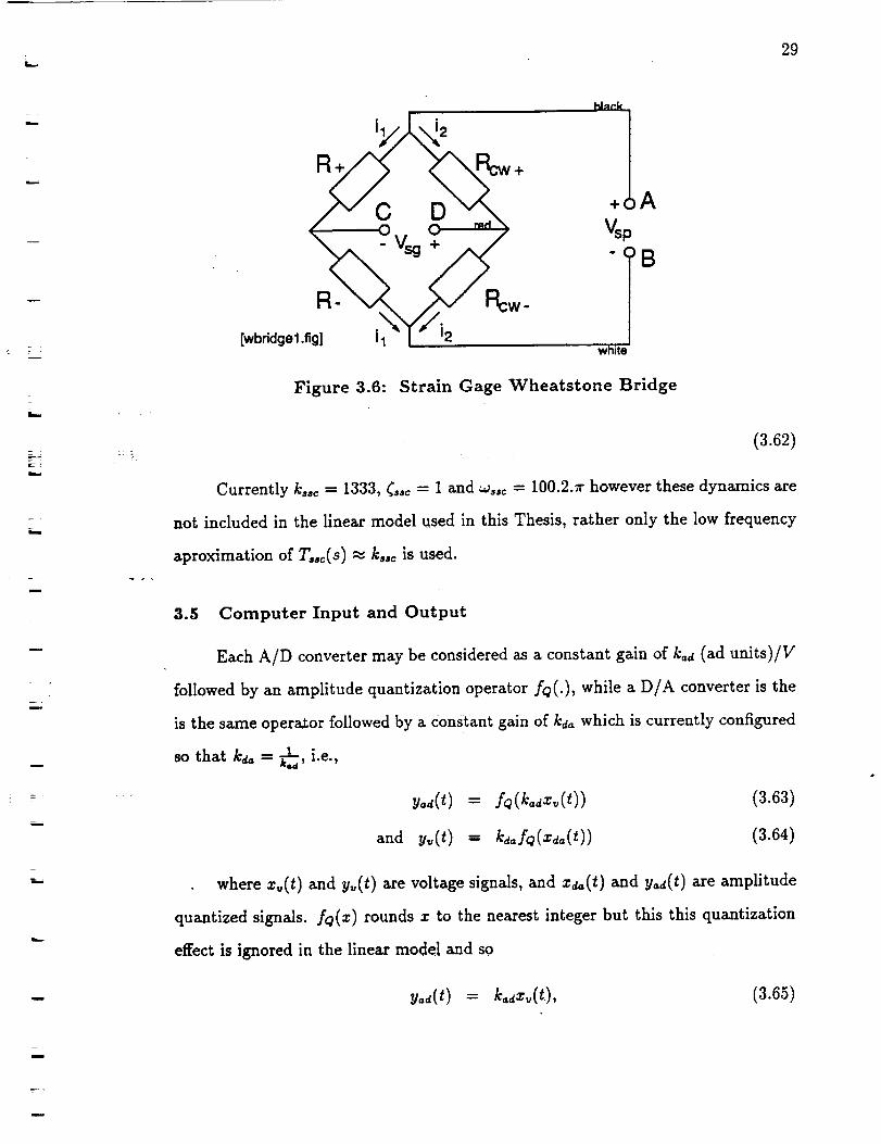
Figure 3.6: Strain Gage Wheatstone Bridge

(3.62)

Currently kooc = 1333, ¢,oc = 1 and _s,c - 100.2.a" however these dynamics are

not included in the linear model used in this Thesis, rather only the low frequency

aproximation of Toot(S) _ k,,, is used.

3.5 Computer Input and Output

Each A/D converter may be considered as a constant gain of k,d (ad units)/V

followed by an amplitude quantization operator fq(.), while a D/A converter is the

is the same operator followed by a constant gain of kd_ which is currently configured

so that k_= 1_-'_d' i.e.,

yad(t)- fQ(kadX,(/)) (3.63)

and y,(t) ffi ka, fQ(zd,(t)) (3.64)

where z_(t) and y,(t) are voltage signals, and z_(t) and y,d(t) are amplitude

quantized signals, fQ(x) rounds z to the nearest integer but this this quantization

effect is ignored in the linear model and so

Y.d(t) = k_dz.(t), (3.65)

r

30

= kd,=d,(t)

assumed ....are

yv(t) (3.66) m

[]

m

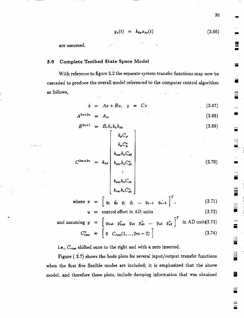
3.6 Complete Testbed State Space Model

With reference to figure 3.2 the separate system transfer functions may now be

cascaded to produce the overall model referenced to the computer control algorithm

._ = (3.67)

A 2"×2_ = (3.68)

B 2"xl = (3.69)

c2mX2n _.

as follows,

Ax + Bu, y = Cx

A,_

B,k k.kd..

k,c ,

k,c ,

k,,,k,C,o

k,,d k,,ok.C:o

ksseksC,4

ksseksCv4

qo qo q, q, ..-

control effort in AD units

[yh_ Y_b Y,0 Y,% .-.

where z =

U --"

and assuming y =

Tq_-t q i ,

(3.70)

(3.71)

(3.72)

in AD unit_3.73)

(3.74)C_,_, = [0 C,_(1,...,2m-2)]

i.e., C_ shifted once to the right and with a zero inserted.

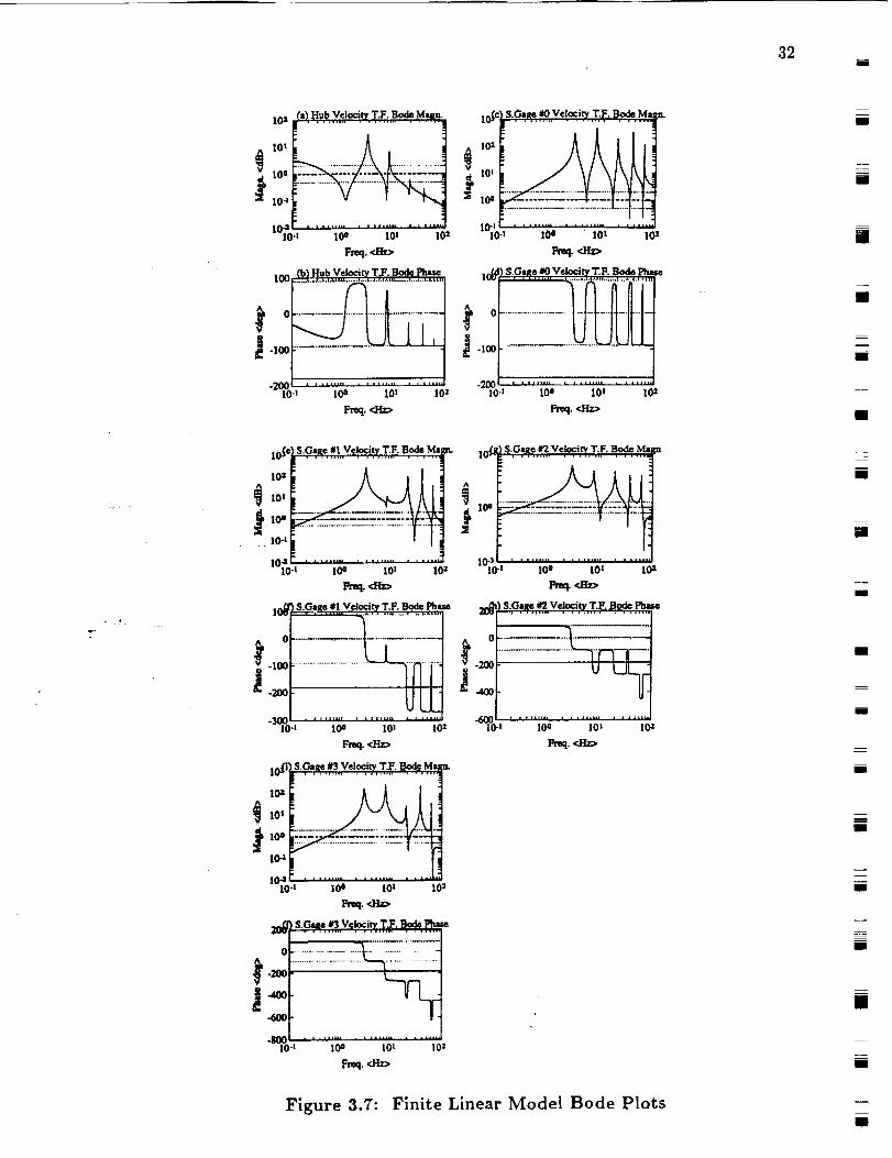
Figure (3.7) shows the bode plots for several input/output transfer functions

when the first five flexible modes are included; it is emphasized that the above

model, and therefore these plots, include damping information that was obtained

i

i

U

i

m

i

i

I

m

i[

!

I

im

m

[]

t

[]

m

i

31

w

w

!

w

m

w

m

w

experimentally, however the form of the plots is invariant wit respect to large es-

timated damping ratio errors. Note that the hub angle velocity transfer function

bode phase plot is bounded by 4-90 degrees as expected because it is strictly positive

real, however so is the phase plot for the first strain gage response even though the

sensor is located a distance of 6.5ram away from the hub along the beam and this is

explained in the next section. All the other strain gage velocity transfer functions

are seen to be not positive real.

3.7 Model Structural Features

Figure (3.8) includes a schematic representation of the plant model which

helps to illustrate the following points.

1. The single input torque simultaneously excites a low pass filter and several

second order filters, while each sensor is a linear combination of the filter

states.

2. The rigid body mode transfer function, torque to q0 is a passive low pass filter,

G6(s) = s/(s + r).

3. Each flexible mode transfer function, torque to q'_, n > 0, is a passive bandpass

filter, G_(s)= 2_iw_sl(s 2 + 2_i_zis + w_).

4. The torque to hub angle velocity transfer function is a positive linear combi-

nation of the Gk(s ) and hence itis minimum phase.

5. In the complete linear model, each torque to strain velocity transfer function

is not strictly positive real and hence there exist negative C,(x) elements

(assuming x > 0). In general the further the strain gage is located from the

hub the "sooner" the first negative C,(x) element occurs for a given number

of modeled modes or, alternatively, for a given non-zero distance from the

32I

X

10= f_ I-Iub Velocity T.F. Bode M_n.

lO°

104

IO1"0.s I0 o 101 10=

l_q. _z>

100 _J'l'ub Velocity T.F. Bode Phase

-100

lO-n 10o lOS 10=

Freq. <Hz>

0.,q

_-1oo

lOn

Oi|/| • ,HH_ u_ .......l I0 a ..... lO t 10.1

en_q. <Hz>

IIZI

"_o-, ..... lo"_,_ 1o_'% lo_

Freq.<m>

A

lO_c

102

1o t

Io o

10-_

1o#

A

I,

0

..6O0

|I01-0"1 10 ° IOs 10=

i

""_0 4 100 I0] 102

$.GaRe _ Velocity T.P. Bode Ma a.!0 _T ...... ,..o . ...............

10 s

10 4 !

r-_q.<m>

10 4 |0 0 tO t 10 2

F.req. <Hz>

_o_ s.._:_.:._v,._.-_.T:.v._. _,,

1_ t ' !0 e 10 t tOz

_req. <Hz_

lO-s 10 • lOS 10z

F-r_q. <Hz_

mm

i

m

i

m

me

i

i

i

2£2

m

mm

i

m

I

i

u

mi

i

i

Figure 3.7: Finite Linear Model Bode Plotsm

33

Plant

Low Pass Filter #0 qv'

, q=.,Band Pass Filter #1 [ q_,

/

i

Band Pass Filter #n-1 q¢,

m

Plant

C

Matri_

I Hub[

St nSt 1

I t _St _

I Tip

fFigure 3.8: Normal Mode Linear Model Structure

=

origin, a negative element will occur in C,(x) for a sufficiently high order

model. However, if the strain gage is close enough to the hub, C,(z) may

contain only positive entries for any given number of beam modes and this is

the case for the first strain gage (#0), which is only 6.5rnm from the hub, and

at least the first five flexible beam modes.

Model Identification

A modal analysis was carried out on the testbed in order to identify the three

sets of finite linear normal mode parameters, i.e.,

1. the first n modal oscillation frequencies (f,_),

2. the corresponding pole damping ratios (_,,),

3. the corresponding input/output gains for each sensor

and the results for fi and _i are shown in table 3.1 for 0 < i < 5. Modal analysis

was used since the test signals may be selected to target individual parameters of

interest, e.g., a sinusoid at a specific flexible mode frequency produces a response

strongly dominated by the corresponding flexible mode and the input/output gains

may now be directly determined. The identified model parameters are considered

34w

more accurate than the analytically derived ones from the beam and hub assembly

physical parameters since some of the latter are only known approximately however

the analytically derived input/output gains gains are used in the final model (i.e.,

the model used for controller design and analysis in the next chapters) since the

identified input/output gain data is not up to date.

3.8.1 Oscillation Frequencies

The first step was to apply a narrowband test signal such as a PRBN function

to the beam and obtain an FFT of any sensor response (although the strain gages

are preferred as the oscillation peaks are well defined) and hence a set of bode plots.

Since each mode is very poorly damped the shape of the sinusoidal response of a

sensor close to an oscillation frequency is strongly determined by the corresponding

modal transfer function and hence the experimentally obtained bode magnitude plot

peak locations determine the oscillation frequencies (and hence the associated pole

magnitudes). A second refined bode magnitude plot was then obtained by applying

individual sinusoids at frequencies close to the estimated pole magnitudes and then

the latter were re-evaluated.

m

iR

I

z

I

I

mu

I

mM

I

mI

3.8.2 Damping coefficients

The rigid body mode non-zero pole was measured by applying a rectangular

input torque and curve fitting the hub angle response in order to determine the rate

of exponential increase (a rectangle rather than a step signal was used since the

latter would of course cause the beam to wind out of its operating envelope). This

mode does not affect the strain gage responses and hence the corresponding strain

gage data cannot be used in order to estimate rigid body mode parameters.

In order to measure the i th flexible mode pole damping ratio (¢_) a sinusoid was

applied at the corresponding center frequency (&i) until a steady state situation was

m

mu

iU

B

B

B

m

J

mm

35

L

w

b

reached and then abruptly removed at time tl; the envelope of each sensor response

after tl exponentially decays with a time constant _/given by

1÷i = _ (3.75)

and once ri is measu'red by curve fitting this envelope (i may be calculated

since wi is known.

3.8.3 Modal Gains

This last set of data also yields the input/output gains bi_j for each sensor j

at each oscillation frequency &i from which the state space model B and C matrices

may be formed.

..... i

3.8.4 Identification Improvements

The above procedures may be improved in order to more accurately identify

system modal parameters and some ideas are as follows.

1. A discrete fourier transform is an estimate of the continuous fourier trans-

form at specific discrete frequencies that are determined by the data sampling rate

and the number of samples. This suggests that a better narrowband signal than

PRBN would be one composed of equal amounts of sinusoids at the discrete fourier

series frequencies with a random constant phase shift applied to each sinusoid in

order to reduce coherent peaks in the time domain signal: unlike PRBN this sig-

nal does not waste energy on frequencies other than those assumed by the discrete

fourier transform (and therefore those of interest) and provides equal weights for

all frequencies. Furthermore, the amplitude weights may be accurately altered if

desired, perhaps to increase the measurement signal/noise ratio at frequencies close

to plant transmission zeros and any number of sinuoids may be omitted in order to

precisely tailor the applied signal bandwidth. This test signal was used for the Bode

plots shown in figure 5.11 which are much smoother than those obtained with PRBN

36 .=

test signals. It may also be possible to specify the individual sinusoid constant phase

shifts rather then set them randomly in order to minimize the maximum test signal

peak in th crime domain so as to further avoid nonlinear response effects associated

with large input signals.

2. Estimate the coulomb friction and include corresponding nonlinear com-

pensation during the identification process. This is particularly important since

test data show significant nonlinear effects when small signals are applied to the

beam and these are assumed to be due to coulomb friction. Furthermore, very large

applied signals also result in nonlinear effects due to nonlinear damping, stiffening

and gravity/torsion effects which may be more easily avoided if smaller signals are

allowed.

3. Calculating complex pole damping ratios by analysing sinusiod decay en-

velopes can be difficult due to nonlinear effects that add unwanted frequencies to

_" "" the data and one possibility is to filter the data with a linear second order band-

pass filter centered at the same modal center frequency first and then the modal

• : damping ratio may be derived from the measured value and that of the bandpass

filter: the center frequency for such a filter is known exactly since it corresponds to

""the applied sinusoid frequency. Another option is to filter the data in a nonlinear

m_anner by applying a window to the corresponding discrete fourier series to select

those frequencies dose to the modal center frequency and then transform back to

the time domain in order to analyse the decay envelope the decaying sinusoid

fourier transform is dominated by frequencies close to its center frequency.

4. The rigid body mode non-zero pole was identified with a rectangular test

.... signal which excites the flexible modes also and though this was taken into account

a better result might be obtained by using a smoother signal, perhaps a rectangular

pulse with parabolic ramping or filtered with a sharp roll off low pass filter.

U

I

m

I

I

I

il

M

=

[]

I

iil

m

m

m

R

g

m

I

R

mIIII

=

w

u

w

w

m

w

L-

CHAPTER 4

Control Design

4.1 Overview

The linear modal flexible beam model developed in chapter three (see equation

(3.67)) possesses a simple decoupted structure , i.e., a collection of second order

systems (a single rigid body mode and the set of flexible modes) driven by a common

input torqe. The rigid body mode largely determines the step response time while

the flexible modes govern the oscillatory behavior and applying feedback control can

decrease the step response time (i.e., move the rigid body mode real poles away from

the origin in the Laplace s domain) and increase the flexible mode damping ratios

(i.e., swing the flexible mode complex pair poles towards the negative real axis in

the Laplace s domain). Applying any amount of hub angle proportional feedback

:moves the pole at the origin and the new closed loop system becomes completely

controllable and observable, hence full state feedback may be used to arbitrarily

place the closed loop poles. However in reality noise, non-linearities and modeling

errors limit the extent to which feedback may be applied and the problem now is

how to select a robust feedback controller.

A useful design tool is the Passivity Theorem (see reference [4]) which guar-

antees that strictly positive real feedback compensation of a positive real (m inputs

and m outputs) plant will produce an asymptotically stable closed loop positive real

system even in the presence of modeling errors, so long as there are no pole-zero

cancellations, and furthermore such a compensator will have an infinite gain margin

when applied to the plant model. In the case of the flexible beam a natural choice

for a positive real (with respect to the input torque) output is the time derivative

of the hub angle which may be obtained with an appropriate sensor, direct filtering

37

w

38I

of the hub angle, or reconstructed from an estimation of the plant states (i.e. using

a closed loop observer). The Passivity theorem may now be applied to show that

hub angle proportional plus derivative (PD) feedback produces an asymptotically

stable closed loop positive real system with an infinite compensator gain margin.

This is the basis of the first controller designed and root locus analysis is used in

a systematic fashion in order to select the actual proportional and derivative gains

as a compromise between rigid body mode performance, flexible mode performance

and pole location sensitivity to gain variations.

However the second and higher order flexible modes are only weakly observable

through the hub angle sensor and in order to substantially increase the damping

ratios of these modes requires unacceptably high PD gains. A solution to this

problem is to synthesize a new positive real output signal, either directly from

several plant sensors (collocated and/or non-collocated) or via an estimate of the

PD compensated plant states, that is strongly coupled to the modes of interest

and then apply a second positive real compensator (see figure 4.5). The Positive

Realness Theorem provides a means for constructing such an output from the PD

compensated plant states and a second controller is designed this way that improves

the damping ratios on the second and third flexible modes using static feedback; a

third controller tested uses a positive real filter in the feedback loop in order decouple

the dynamics of higher order uncompensated modes.

Each of these controllers is designed using a four mode plant model (eight

states) and an observer to provide an estimate of the plant states from which positive

real outputs are generated. The effect of some unmodeled higher order modes on

the positive realness of synthesized plant outputs is examined (through simulations)

with different closed loop observer types, namely, full order pole placement, reduced

order Luenberger pole placement and LQE designs and the observer which produces

an output least sensitive to the modeling error is selected: open loop observers are

g

g

m

M

_.k_

m

i

m

I

R

m

W

m

i

m

m

mm

I

39

not tested.

When designing and testing compensators a mixed analytical/identified model

was used since the identified model parameters are considered more accurate than

the analytically ones derived from the beam and hub assembly physical parameters

(see chapter 3).

4.2 Positive Realness

With reference to [2], assume a minimal (controllable and observable) expo-

nentially stable system E with time domain representation

_(t) = Az(t) + Bu(t), x(O) = Zo

y(t) = cz(t) + D,,(t) (4.1)

b

w

and frequency domain representation

y(s) = (D + C(sI- A)-lB)u(s) = T(s) (4.2)L ' - :L

where z e _n, u, y E _'_ and a,_i,_(B) > 0.

Theorem la :

(A, B, C, D) is Strictly Positive Real if there exists P > 0 , P , L E _"×" ,

_,_i.(L) _ , _'×" _'×"= e > 0 Q E , and W E that satisfy the Lur'e equations

Arp_. pA = -Q:rQ - L (4.3)

Brp- C = WrQ (4.4)

WrW = D + D T. (4.5)

r

For the flexible beam model (3.67) D is null and so we may take W and Q to

be null in which case the above three equations reduce to

AT p + PA = -L

C = BTp.

(4.6)

(4.7)

40 m

This theorem offers a method of computing an output matrix C in terms of

L such that the corresponding system is positive real as follows : equation 4.6 is a

Lyapunov matrix equations and since/J,_a=(A) < 0 (e.g., _ is a minimal exponen-

tially stable system) there exists a unique solution P for any given L (see [5], page

574) which may be expressed as

co T

P -- [ eA tLeAt (4.8)J0

Furthermore, _ : = :-

m

i

m

!

mm

L>0 and L*=L =_ P>0 and P*=P. (4.9)

Therefore BTp(sI - A)-IB will be a positive real transfer function if L is_.

restricted as in 4.9. In practice equation 4.8 is not suitable for computer computation

but other more efficient methods exist and are readily available (e.g., the LYAP

function in MATLAB).

Physically, L determines the convergence rate of the Lyapunov function V(x) =_

x*Px w.r.t, the open loop plant since

d v(x(t)) = -.'(t)Lx(t) (4.1o)

along any solution trajectory of _ = Az.

Now, if D is null, the equivalent frequency domain conditions for positive

realness axe:

Theorem 2b : T(s) is Strictly Positive Real if for all w E

ml1

m

mm

mm

_z

mm

mm

mm

m

I

mm

I

and

T(jw)+T°(jw) > 0 (4.11)

Jim ¢v2(T(jw) + T°(jca)) > 0 (4.12)

Hence a Nyquist plot for a positive real transfer function will lie in the closed

right half complex plane while a bode phase plot will be bounded by 4-90 deg. All

i

mg

I

m

m

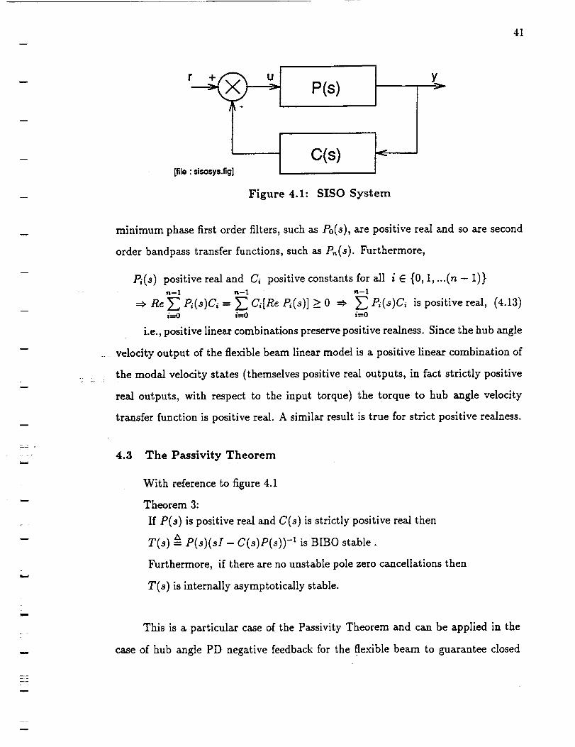
41

[file : sisosys.fig]

P(s)

c(s)

Y

Figure 4.1: SISO System

minimum phase first order filters, such as P0(s), are positive real and so are second

order bandpass transfer functions, such as P,,(s). Furthermore,

P_(s) positive real and C_ positive constants for all i E {0,1,...(n-1)}n--1 n--1 n--1

=_ Re __, P,(s)C, = _ C,[Re P,(s)] _> 0 => _ P,(s)C, ispositive real, (4.13)i=0 i=O i----O

i.e., positive linear combinations preserve positive realness. Since the hub angle

velocity output of the flexible beam linear model is a positive linear combination of

the modal velocity states (themselves positive real outputs, in fact strictly positive

real outputs, with respect to the input torque) the torque to hub angle velocity

transfer function is positive real. A similar result is true for strict positive realness.

L--

r

i

m

4.3 The Passivity Theorem

With reference to figure 4.1

Theorem 3:

If P(s) is positive real and C(s) is strictly positive real then

T(s) _ P(s)(sI - C(s)P(s))-' is BIBO stable.

Furthermore, if there are no unstable pole zero cancellations then

T(s) is internally asymptotically stable.

This is a particular case of the Passivity Theorem and can be applied in the

case of hub angle PD negative feedback for the flexible beam to guarantee closed

w

42

loop asymptotic stability assuming a non-zero derivative gain and more generally

any collocated actuator and velocity sensor pair will produce a positive real transfer

function for a mechanical structure that includes: no energy sources.

Note that the Passivity Theorem is sufficient but not necessary; less restrictive

conditions based upon the open loop plant may be developed from the Nyquist

stability criterion which is itself a necessary condition.

I

J

l

u

4.4 Hub Angle PD Compensator

The hub angle forward path PD compensator is designed in two stages; firstly

only the rigid body mode of the plant is modeled and a two column matrix of

increasing PD gains is obtained analytically corresponding to increasing closed loop

step response performance. Secondly the modeled flexible modes are included and

a particular pair of PD gains is selected based on ti_e characteristic equation root

locus plot. While pole location sensitivities w.r.t, compensator parameters are also

considered no attempt is made to analytically or numerically optimize a performance

and/or robustness index.

4.4.1 Closed Loop Stability

Figure 4.2 (a) shows the flexible beam plant (torque to hub angle) with a

PD feedback compensator. By transferring the plant integrator to the compensator

block as in part (b) of the figure the modified plant becomes strictly positive real

while the compensator becomes positive real (and strictly positive real for d > 0)

and hence the Passivity Theorem guarantees asymptotic stability of the the closed

loop system.

I

I

M

I

m

m

l

1

I

M

l

J

m

I

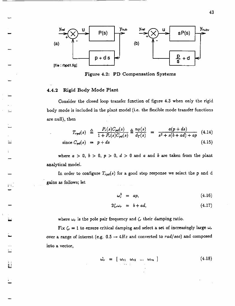
43

=

=

£ •

w

w

g

w

__4

m

= =

(a)

[fiFe : rbl_l .fig]

P(s)

_t p+ds

Figure 4.2:

b yref f

(b)

sP(s)

PD Compensation Systems

bv

4.4.2 Rigid Body Mode Plant

Consider the closed loop transfer function of figure 4.3 when only the rigid

body mode is included in the plant model (i.e. the flexible mode transfer functions

are null), then

T._,d(S) " P_(s)Cpd(s) _ nT(s) a(p + ds) (4.14)= 1+P.(_)c_,(_) =d_(_-----_= _+_(b+.d)+.p

sinceC_(s) = p + ds (4.15)

where a > O, b > O, p > O, d > 0 and a and b are taken from the plant

analytical model.

In order to configure T, pd(s) for a good step response we select the p and d

gains as follows; let

2wr = ap,

2_rCa, = b+ad,

where _, is the pole pair frequency and _ their damping ratio.

(4.16)

(4.17)

Fix ¢'_ = 1 to ensure critical damping and select a set of increasingly large w,

over a range of interest (e.g. 0.5 --* 4Hz and converted to rad/sec) and composed

into a vector,

m

44I

then equations 4.16 and 4.17 imply that

2

Pi = w_-'i (4.19)a

di = (4.20)a

,o],

where 15 and d are the n x 2 P and D monotonically increasing gains which

correspond to _. The higher the values of pi and di the higher is w_i and the faster

the closed loop step response. Note that the minimumw_ considered (i.e., for i = 1)

is determined by equation (4.20) as

0Jrl

b= -- (4.23)

26

in order to avoid any negative values for di since this may result an unstable

T,

I

I

m

zI

m

I

I

=!

,4.4.3 Root Locus Design : _

The second step is to add the flexible modes to the plant model to produce

P(s) as shown in figure 4.3 while maintaining the rigid body mode PD compensator

class subject to the constraints of equations (4.19) and (4.20) so that the new

torque to hub angle transfer function Tpd(s) is given by,

P(s) nT(s) (4.24)Tpa(s) = 1 + P(s)Cpa(s) = dT(s'-"'_

and the PD compensator may be expressed as

u - r - (p.BTitt + d.BT)z (4.25)

T f"since Yh_ = Bshi/t z and yh,_,, = y[Lub = BTx (4.26)

r A [ ] (4.27)where B,hiSt = B(2) B(3)... B(n) 0

m

mi

i

m

m

mJ

u

J

m=

B

=

m

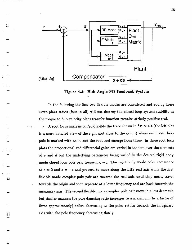
45

m_

m

[fullpdl .fig]

Um

. ;IR Mo°e

F Moden-1

Plant

Chub

Matrix

Plant

Compensator t p+ds <

Figure 4.3: Hub Angle PD Feedback System

Yhub

E

m

==

- m

i

= ,

n

In the following the first two flexible modes are considered and adding these

extra plant states (four in all) will not destroy the closed loop system stability as

the torque to hub velocity plant transfer function remains strictly positive real.

: : A root locus analysis of dT(s) yields the trace shown in figure 4.4 (the left plot

is a more detailed view of the right plot close to the origin) where each open loop

pole is marked with an x and the root loci emerge from these. In these root locii

plots the proportional and differential gains are varied in tandem over the elements

of/_ and d but the underlying parameter being varied is the desired rigid body

mode closed loop pole pair frequency, w_i. The rigid body mode poles commence

at s = 0 and s - -a and proceed to move along the LHS real axis while the first

flexible mode complex pole pair arc towards the real axis until they meet, travel

towards the origin and then separate at a lower frequency and arc back towards the

imaginary axis. The second flexible mode complex pole pair move in a less dramatic

but similar manner; the pole damping ratio increases to a maximum (by a factor of

three approximately) before decreasing as the poles return towards the imaginary

axis with the pole frequency decreasing slowly.

= =

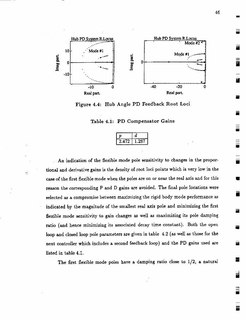
46qJ

tJ

10

0

-10

Hub PD System R.Locus

. )° .o°'"*"

I

• Mode #1

,•°

•°,°°.°.

-I0 0

Real part.

0

Hub PD System R.Locus' ' Mode #2 'c_

Mode #1 ....• ....

,_,,w

.L.,_".

•°

I I

-40 -20

Real i_--t.

Figure 4.4: Hub Angle PD Feedback Root Loci

Table 4.i: PD Compensator Gains

p d

2.472 1.287

i

[]

[]

[]

m

I

im

m

=

=

I

_7

An indication of the flexible mode pole sensitivity to changes in the propor-

tional and derivative gains is the density of root loci points which is very low in the

case of the first flexible mode when the poles are on or near the real axis and for this

reason the corresponding P and D gains are avoided. The final pole locations were

selected as a compromise between maximizing the rigid body mode performance as

indicated by the magnitude of the smallest real axis pole and minimizing the first

flexible mode sensitivity to gain changes as well as maximizing its pole damping

ratio (and hence minimizing its associated decay time constant). Both the open

loop and closed loop pole parameters are given in table 4.2 (as well as those for the

next controller which includes a second feedback loop) and the PD gains used are

listed in table 4.1.

The first flexible mode poles have a damping ratio close to 1/2, a natural

E

11

m

I

m

m

=

I

I

N

mE

[]

EE

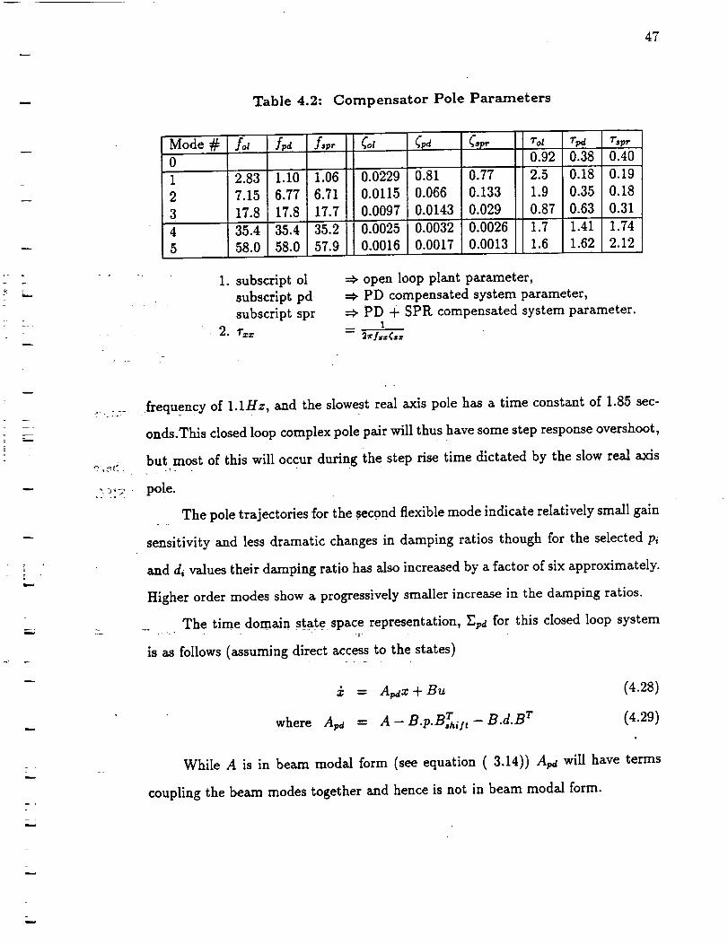
47

Table 4.2: Compensator Pole Parameters

Mode #

0

1

2

3

4

5

.

2.83 l.lO 1.06

7.15 6.77 6.71

17.8 17.8 17.7

35.4 35.4 35.2

58.0 58.0 57.9

subscript ol

subscript pd

subscript spr

r==

Gd

0.0229 0.81 0.77

0.0115 0.066 0.133

0.0097 0.0143 0.029

0.0025 0.0032 0.0026

0.0016 0.0017 0.0013

Tol

0.92

2.5

1.9

0.87

1.7

1.6

T_4 rsvr

0.38 0.40

o.i8 o.190.35 0.18

0.63 0.31

1.41 1.74

1.62 2.12

=_ open loop plant parameter,

=> PD compensated system parameter,

=_ PD + SPR compensated system parameter.1

z=

. =.__

bm

:..:.;_ frequency of 1.1Hz, and the slowest real axis pole has a time constant of 1.85 sec-

onds.This closed loop complex pole pair will thus have some step response overshoot,

_, butmost of this will occur during the step rise time dictated by the slow real axis

- ;,; pole.

The pole trajectories for the second flexible mode indicate relatively small gain

sensitivity and less dramatic changes in damping ratios though for the selected p_

and d_ values their damping ratio has also increased by a factor of six approximately.

Higher order modes show a progressively smaller increase in the damping ratios.

_. The time domain state space representation, _va for this closed loop system

is as follows (assuming direct access to the states)

-'- A_x + Bu (4.28)

where Ava -- A - B.p.BTqt - B.d.B r (4.29)

While A is in beam modal form (see equation (3.14)) Apa will have terms

coupling the beam modes together and hence is not in beam modal form.

-

4.5 Synthesized Positive Real Output Controller (static feedback)

48

The hub angle PD compensation feedback loop designed above is a form of full

state feedback that provides good rigid body mode response with little or no over-

shoot, approximately critically damps the first flexible mode and offers an infinite

gain margin in the exact model case. However the higher order closed loop flexible

modes remain relatively poorly damped (see table 4.1) and in order to add further

damping to these flexible modes we can modify the PD full state feedback gains by

closing a second feedback loop ; the following gain selection approach makes use of

the time domain state space representation definition of strict positive realness in

order to guarantee an infinite gain margin and a phase margin of [-90, 90] degrees

for this second loop. In this example the exact gains are selected through trial and

error, however there is a strong correlation between individual gain magnitudes (in

a parametric form) and the corresponding closed loop flexible mode damping ratios

:, :_: r: which simplifies the selection process.

, ATheorem la implies that open loop system P_,.(s) BTpxpd(S) (where

X_(s) _= (sI- Apd)-lB) will be a strictly positive real transfer function (and SISO

" since B is a column vector) if the square matrix P is the unique solution to

(4.30)

.r

TApaP + PApa = -L

where L>0 and L'=L

and the Passivity Theorem then guarantees that the close loop system Tsp,(s) _-

P_(s)[I + P,p_(s)]-' will be BIBO stable with an infinite gain margin.

With regards to figure 4.5 Xpd(S) is the torque reference (r(s)) to PD compen-

sated plant state vector transfer function and Cspm _- BTp is the output matrix

synthesized specifically for this system so as to produce the SPR SISO transfer

function Psp,.(s), and since only static negative feedback is applied the correspond-

ing closed loop system T,p_(_) will have a phase margin of at least [-90, 90] degrees.

m

|!I

I

R

mm

g

m

m

[]

mI

m

B

[]

i

I

[]

[]

m

m

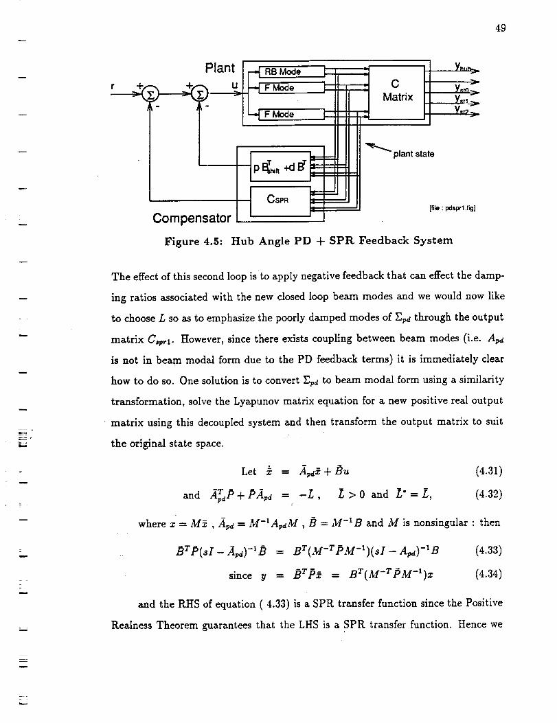
49

!

w

n

m

Plant

Compensator

RB Mode

F Mode

Mode

CSPR

i y,. __Matrix

plant state

[file : I:<lsprl.fig]

Figure 4.5: Hub Angle PD -JrSPR Feedback System

The effect of this second loop isto apply negative feedback that can effect the damp-

ing ratios associated with the new closed loop beam modes and we would now like

to choose L so as to emphasize the poorly damped modes of Zpd through the output

matrix C,p_l. However, since there exists coupling between beam modes (i.e. A_

is not in beam modal form due to the PD feedback terms) it is immediately clear

how to do so. One solution is to convert Zpa to beam modal form using a similarity

transformation, solve the Lyapunov matrix equation for a new positive real output

matrix using this decoupled system and then transform the output matrix to suit

the original state space.

Let = 2,d + [3u (4.3z)

and fiirdP + Pftpd = -L, Z, > 0 and L* = L, (4.32)

where x = M_. , fipd = M-1A_M , [3 = M-X B and M is nonsingular : then

[3Tp(SI -- ipd)-l [3 =

since y =

BT(M-T.pM-1)(sI - A_)-IB (4.33)

[3Tp£. = BT(M-TpM-Z)x (4.34)

and the RHS of equation (4.33) is a SPR transfer function since the Positive

Realness Theorem guarantees that the LHS is a SPR transfer function. Hence we

±

w

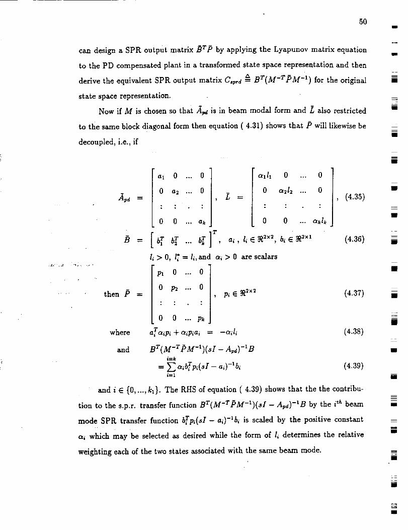
5OI

can design a SPR output matrix/2rp by applying the Lyapunov matrix equation

to the PD compensated plant in a transformed state space representation and then

derive the equivalent SPR output matrix C,p,d _- Br(M-rPM =1) for the original

state space representation.

Now if M is chosen so that fi,_ is in beam modal form and L also restricted

to the same block diagonal form then equation (4.31) shows that/5 will likewise be

decoupled, i.e., if

2_pd

/2

then 15 _

where

al

0

0

0

a2

0

... 0

,.. 0

•.. ale

... ]Tbr

L __

c_1ll 0 ...

0 c_212 ...

0 0 ... aklk

ai , li E R 2×2, biER2×1

li>O, l*-li, and ai > 0 axe scalars

Pl 0 ...

0 _ ...

: : :

0 0 ... pk

a raipi + cqpiai

0

0, pi E R 2x2

0

0(4.35)

(4.36)

(4.37)

-- -all{ (4.38)

and BT(M-TpM-1)(sI- Apa)-_Bi=1¢

=Z:-,bTp,( r - .,)-'b,i=1

(4.39)

and i E {0, ..., kt}. The RHS of equation (4.39) shows that the the contribu-

tion to the s.p.r, transfer function BT(M-rpM-t)(sI - Apa)-tB by the i th beam

mode SPR. transfer function brpi(sI - ai)-Ibi is scaled by the positive constant: :5 ;

ai which may be selected as desired while the form of Ii determines the relative

weighting each of the two states associated with the same beam mode.

m

I

=_

Ill

I

l

II

I

l

I

=

ll

I

I

I

I

I

I

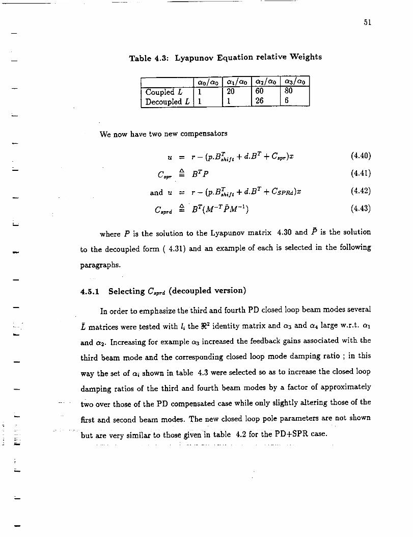
51

Table 4.3: Lyapunov Equation relative Weights

_o/_o _,/ao ..a2/ao a3/_oCoupled L 1 20 60 80

Decoupled g 1 1 26 6

=

We now have two new compensators

u = r - (p.BT,f, + d.S r + C._,)_ (4.40)

C_p, _- BTp (4.41)

and u = r - (p.BT,ft ÷ d.B T ÷ CSPRd)X (4.42)

C_p,d _- BT(M-rpM -') (4.43)

where P is the solution to the Lyapunov matrix 4.30 and P is the solution

to the decoupled form (4.31) and an example of each is selected in the following

paragraphs.

4.5.1 Selecting C_p_d (decoupled version)

In order to emphasize the third and fourth PD closed loop beam modes several

L matrices were tested with li the _2 identity matrix and a3 and a4 large w.r.t. 01

and a2. Increasing for example a3 increased the feedback gains associated with the

third beam mode and the corresponding closed loop mode damping ratio ; in this

way the set of ai shown in table 4.3 were selected so as to increase the closed loop

damping ratios of the third and fourth beam modes by a factor of approximately

two over those of the PD compensated case while only slightly altering those of the

first and second beam modes. The new closed loop pole parameters are not shown

hut are Very similar to those s,-_'-_in table 4:2 forthe PD+SPI_ case.: :

52m

=r. -

4.5.2 Selecting C_p_ (coupled version)

For the SPR output design based UP0 n the or!g!nal coupled system EpD the

form of L chosen was" that of _, in the previous example (i.e., as in equation (4.35)

with l_ the _u identity matrix) with again small values for ch and a2 and large

values for a3 and a4. Although there is no longer an exact correlation between cri

and the contribution of each beam mode of EpD to the synthesized SPR output

there is an approximate effect if the intermodal coupling is small as is the case for

the third and higher order flexible beam modes. Again ct3 and _4 were selected so

as to increase the closed loop damping ratios of the third and fourth beam modes

by a factor of approximately two over those of the PD compensated case while only

slightly altering those of the first and second beam modes and the results are shown

in table 4.2 while the relative values for c_ are given in table 4.3

4.6 State Estimation

The experimental testbed currently contains a hub angle sensor and four beam

strain gages : any other output such as a velocity signal or a synthesized passive

output must be obtained by direct filtering of the existing outputs or reconstructed

from an observer estimate of the plant states. The latter was chosen so as to

provide a complete plant state estimate from which any desired output may be

generated. Under ideal conditions a close match may be obtained between the

actual and estimated state within the bandwidth of the observer, however modeling

errors and unmodeled features can distort the estimated state and in this section

we look at such effects due to several uncompensated beam modes (i.e., some higher

order beam modes not modeled at the compensator design stage) in the presence of

three different types of closed loop observers. In particular, we apply PD negative

feedback based upon the estimated state of kl beam modes and then examine the

transfer function from the single torque reference signal to the single synthesized

mm

_m

m

Is

mm

[]

|

B

I

I

m

J

mm

m

mm

mm

I

m

m

[]

mm

m

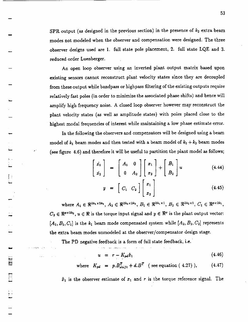
53

w

m

m

n

,s

SPR output (as designed in the previous section) in the presence of k2 extra beam

modes not modeled when the observer and compensation were designed. The three

observer designs used are 1. full state pole placement, 2. full state LQE and 3.

reduced order Luenberger.

An open loop observer using an inverted plant output matrix based upon

existing sensors cannot reconstruct plant velocity states since they are decoupled

from these output while bandpass or highpass filtering of the existing outputs require

relatively fast poles (in order to minimize the associated phase shifts) and hence will

amplify high frequency noise. A closed loop observer however may reconstruct the

plant velocity states (as well as amplitude states) with poles placed close to the

highest modal frequencies of interest while maintaining a low phase estimate error.

In the following the observers and compensators will be designed using a beam

model of kl beam modes and then tested with a beam model of kt + k2 beam modes

(see figure 4.6) and therefore it will be useful to partition the plant model as follows;

i 1]:[A10]f ll[ 11+_2 0 A2 x_ B2

where At E _2k_×2k_ , A2 E R2k2×2k_ , B1 E _2k, x,1

u (4.44)

(4.45)

, B2 E N2k2×l, C1 E Rp×2k,,

C2 E _v×2k2, u E _ is the torque input signal and y E _P is the plant output vector:

[At, B1, C1] is the kt beam mode compensated system while [A2, B2, C_] represents

the extra beam modes unmodeled at the observer/compensator design stage.

The PD negative feedback is a form of full state feedback, i.e.

u = r- I{#_, (4.46)¢

where Kva r= P.B,hll _ + d.B r ( see equation (4.27) ), (4.47)

_t is the observer estimate of zt and r is the torque reference signal. The

L_

w

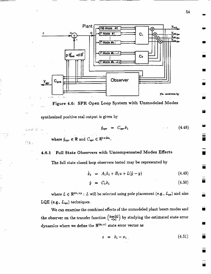
54m

_ k

= £

Plant

U•

RB Mode #0

-..L F Mode #1

-_ F Mode #1e +k =

Observer I[_, :=._.f_]

: Figure 4.6: SPR Open Loop System with Unmodeled Modes

synthesized positive real output is given by

9,_ = C.p-_l

where 9.n,. E _ a,nd C,_,. E _ ' x21`'.

(4.48)

4.6.1 Full State Observers with Uncompensated Modes Effects

The full state closed loop observers tested may be represented by

z_ = A1,_1+ B_u+ L(_).- y) (4.49)

(4.50)

where L E _2kl ×p : L will be selected using pole placement (e.g., Lpv ) and also

LQE (e.g., Ltq,) techniques.

We can examine the combined effects of the unmodeled plant beam modes and

the observer on the transfer function (v,_m_ by stud_ng the estimated state errork "(=) )

dynamics where we define the _2k_ xl state error vector as

e = _l-zl (4.51)

I

=--

I

=

I

I

i

I

I

Bm

!

i

==

z

I

I

i

I

=

55

Equations (4.51), (4.44) and (4.46) imply that

yprCs) = C, pr$l(s) = C, prT_pd(s)r(s)+C,p,T_,(s)e(s) (4.52)

where T,,,_(s) _- (sI-Al,a)-'B1, (4.53)

T,i(s) _- I + (sI- AI,d)-XB1K, d, (4.54)

and Ai,,a _ A1-B1K,,_. (4.55)

Tlpd(s) is the designed PD closed loop transfer function (torque reference to

modeled plant state) while T_,_ (s)e(s) represents the associated (e)rror dynamics for

the (i)deal case which in the absence of unmodeled beam modes will be exponentially

stable and decoupled from v since equations (4.49) and (4.51) show that

m

m

=--,

= Aoe (4.56)

where Ao _ A1 + LC1. (4.57)

Now when unmodeled beam modes axe included in the plant e is driven by the

extra plant states x_ and the corresponding error equation is given by

where

= Aoe- LC2x2

or e(s)= -T._I(s)_:(s),

T._;(s) = (sI- Ao)-ILC2.

(4.5s)

(4.59)

(4.60)

(4.61)

T_! is the transfer function between the (u)nmodeled plant states and the

modelled state (e)rror vector for the (f)ull state observer case.

Lastly, combining equations (4_59), (4.46) and (4.52) yields

C'._,(s) =

where T.(s) -

and T2pd(s)

C,_T,_(s)[I + (I - T_(s)Kpd)-'T_(s)Km]r(s) (4.62)

T_(s)T_/(s)T2,a(s) (4.63)

is the unmodeled state counterpart to Tl_(s)

56U

i.e. T2pa(s) = (sI- A2va)-lB2 (4.64)

where A2pd = A2 - B2Ifpd (4.65)

Equation (4.62) shows the effect of the unmodeled dynamics (i.e., T:p_(s)) on

the synthesized positive real output Cs v, x(s) (which of course may no longer be

strictly positive real): if T:vd(s ) is null then this equation reduces to the ideal case

(i.e equation 4.52 with zero error initial conditions). It is desirable to maintain the

positive realness of C_w,$l(s) in order to preserve the associated obtainable gain and

phase margins when this second feedback loop is closed and hence equation (4.62)

suggests that L and C_r_ be selected so as to maximize

=

I

i

[]

|

mm

l

m

II

inf Re(C,p_Txpd(jw)[I + (I - T_(jw)Ifva)-_T_(jw)Kvd]r(jw)) (4.66)¢aER

(as well as to meet other observer design criteria and emphasize selected beam

modes).

4.6.2 Reduced Order (Luenberger)'Observer with Uncompensated Modes

Effects

The reduced order (Luenberger) observer may be represented by

where A_oT

zl = A_oz, + Eu + Gy (4.67)-1

= TA_ - GC_, (4.69)

E _ TBx (4.70)

and T is also constrained such that [ C1 ] is nonsingular.

[ T ]The analysis of the previous section may be carried out in order to determine

the transfer function relating the torque reference r(s) to the synthesized SPR output

m

M

i

tm

m

m

[]

=

m

I

mI

m

I

W

I

m

I

W

57

w

C.p,_,(s) with only one change, namely the relationship between z2 and e. Unlike

the full state observer case the term _l(s). does not appear explicitly in the reduced

order observer state equations so we work with the linear combinations that do,

namely Cx_,(s) ( = y ) and T_(s) ( = z ) and relate these to e and then equation

(4.68) gives the desired transfer function.

Clxl -- y -- Clzl q'C'2z2 (4.71)

=_ C,e - C2x2 (4.72)

and equations (4.67), (4.69), (4.70) and 4.51 imply that

T_ = _,- T:zl = A_oTe + GC2z2 (4.73)

Te(s) = (sI- A,O)-_GC2x2 (4.74)

m

EF

w

Combining (4.51), (4.68), (4.72) and (4.74) gives

=2 ¸ .. _t .? "

ww

C1

T

C,

T

-1

C,e(s)Te(8) ]

-1

(sI - A,o)-IG

(4.75)

C2x2(s) _ T_,_,(s)x2(s). (4.76)

T,_,.(s) (r for (r)educed order Luenberger observer) may now replace T,_.t(s)

in equation (4.62) above to give the new r(s) to C_,,,.&,(s) transfer function when

the unmodeled beam modes are included.

n

F_

CHAPTER 5

Simulation and Experimental Results

m

m

g

In the previous chapter two controllerswere developed for the analyticallinearmodel

of the flexiblebeam, PD and PD plussynthesized strictlypositiverealfeedback, and

in the followingsection the step responsesof the corresponding closed loop systems

axe examined using both linearmodel simulations and experimental tests on the

actual testbed (and therefore in the presence of unmodeled linearand non-lineax

dynamics and noise).Also, distortioneffectsunder the three closed loop observers

axe evaluated and the best observer selected.

The compensators and observersare converted to discreteform using the bilin-

ear Tustin transformation and a sampling frequency of 500Hz which isover twenty

fivetimes higher than the highest compensated beam modal frequency : the same

descretizedmodels are used for both computer simulations and experimental tests.

In each case referencetrajectoriesaxe applied in the form of open loop plant modal

states.

In each casethe closedloop system structureisvery similarto that of the open

loop plant;e.g.,the hub angle PD and passivitybased feedback systems contain a

rigidbody mode (though there isno longer a pole at the origin)and flexiblemodes

with new center frequenciesand damping ratios.

i

II

m

mm

mm

H

m

m

llm

[]

m

i

lib

5.1 Simulation Results with Ideal Observer

The PD full state controller designed in the previous chapter provides a good

rigid body mode response and large damping for the Second closed loop flexible

mode. However higher order closed loop flexible beam modes remain poorly damped

and a second feedback loop based upon a synthesized strictly positive real output is

used to increase the corresponding damping ratios by a factor of two approximately

58

z

i

m

I

i

Ill

m

mU

mm

BII

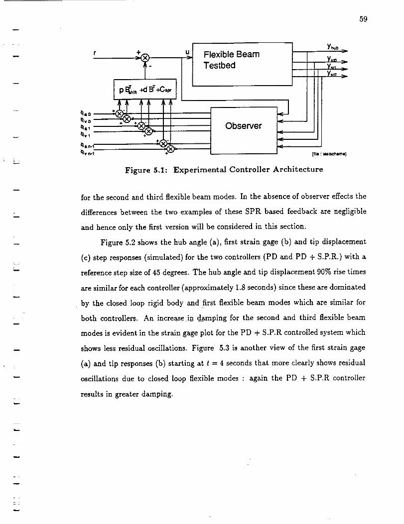
59

rI p I_,. -,'-dB'r+cw

qvo

qal

qvl

qan-1

qvn-;

Flexible Beam

Testbed

Observer

Y_

I Y_M

[file : mstscheme]

Figure 5.1: Experimental Controller Architecture

w

for the second and third flexible beam modes. In the absence of observer effects the

differences between the two examples of these SPR based feedback are negligible

and hence only the first version will be considered in this section.

Figure 5.2 shows the hub angle (a), first strain gage (b) and tip displacement

(c) step responses (simulated) for the two controllers (PD and PD + S.P.R.) with a

reference step size of 45 degrees. The hub angle and tip displacement 90% rise times

axe similar for each controller (approximately 1.8 seconds) since these are dominated

by the closed loop rigid body and first flexible beam modes which are similar for

both controllers. An increase in damping for the second and third flexible beam

modes is evident in the strain gage plot for the PD + S.P.R controlled system which

shows less residual oscillations. Figure 5.3 is another view of the first strain gage

(a) and tip responses (b) starting at t = 4 seconds that more clearly shows residual

oscillations due to closed loop flexible modes : again the PD + S.P.R controller

results in greater damping.

w

w

L

m

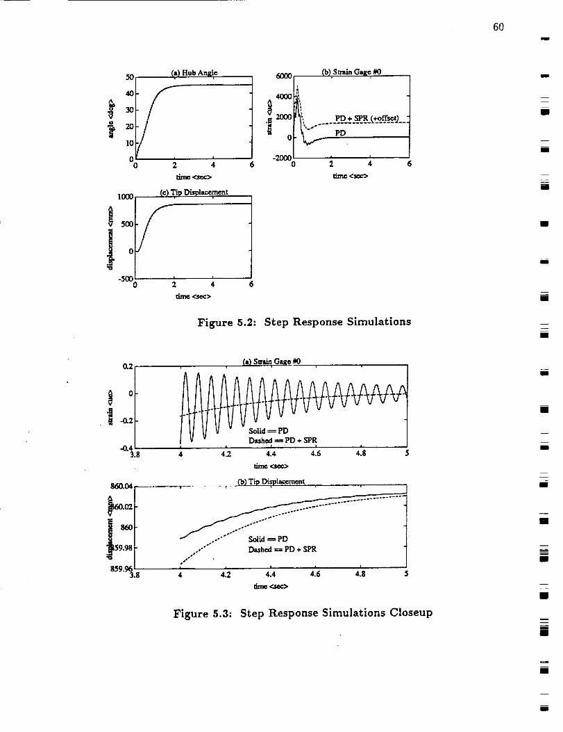
50

40

L' 20lO

00

1000

5OO

0

(a) Hub Angle, +

(!

_ <see_

SI

"5°00 :2 4

time ,<,s_>

6000

400G

._ 2000

0

-20006 0

(b)Strain Oa_e _R)

J

PD + SPR (+offset)i .........._.___.._.___

___ PD

Figure 5.2: Step Response Simulations

(X2

0

-0.43.8

860.04

9.98

859.963,8

+ (=)sa_,one_o

Dashed --_ PD + SPRI ,, I | i

4.2 4.4 4.6 4.8

time <._¢>

(b) Tip Di_lacernem

//"" Dashed = PD + SPR

+ +12 +14. ,+.6 I

4.8 5

Figure 5.3: Step Response Simulations Closeup

I

I

I

m

lg

I

i

m

II

iI

lira

a

iI

m

!

J

i

mm

I

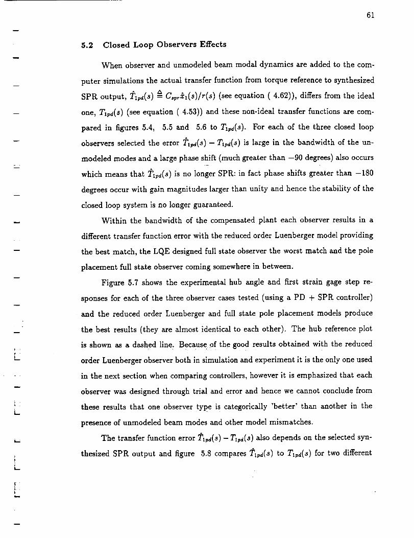
m

L

i

61

5.2 Closed Loop Observers Effects

When observer and unmodeled beam modal dynamics are added to the com-

puter simulations the actual transfer function from torque reference to synthesized

SPR output, Tlpa(s) a= Cspr_(s)/r(s) (see equation (4.62)), differs from the ideal

one, Txpa(s) (see equation (4.53)) and these non-ideal transfer functions are com-

pared in figures 5.4, 5.5 and 5.6 to Ti_a(s). For each of the three closed loop

observers selected the error _blpd(s) - Tl_(s) is large in the bandwidth of the un-

modeled modes and a large phase shift (much greater than -90 degrees) also occurs

which means that _'Ipa(s) is no longer SPR: in fact phase shifts greater than -180

degrees occur with gain magnitudes larger than unity and hence the stability of the

closed loop system is no longer guaranteed.

Within the bandwidth of the compensated plant each observer results in a

different transfer function error with the reduced order Luenberger model providing

the best match, the LQE designed full state observer the worst match and the pole

placement full state observer coming somewhere in between.

Figure 5.7 shows the experimental hub angle and first strain gage step re-

sponses for each of the three observer cases tested (using a PD + SPR controller)

and the reduced order Luenberger and full state pole placement models produce

the best results (they are almost identical to each other). The hub reference plot

is shown as a dashed line_ Because of the good results obtained with the reduced

order Luenberger observer both in simulation and experiment it is the only one used

in the next section when comparing controllers, however it is emphasized that each

observer was designed through trial and error and hence we cannot conclude from

these results that one observer type is categorically 'better' than another in the

presence of unmodeled beam modes and other model mismatches.

The transfer function error Tx_(s) - T1p_(S) also depends on the selected syn-

thesized SPR output and figure 5.8 compares T_pd(s) to T_pd(s) for two different

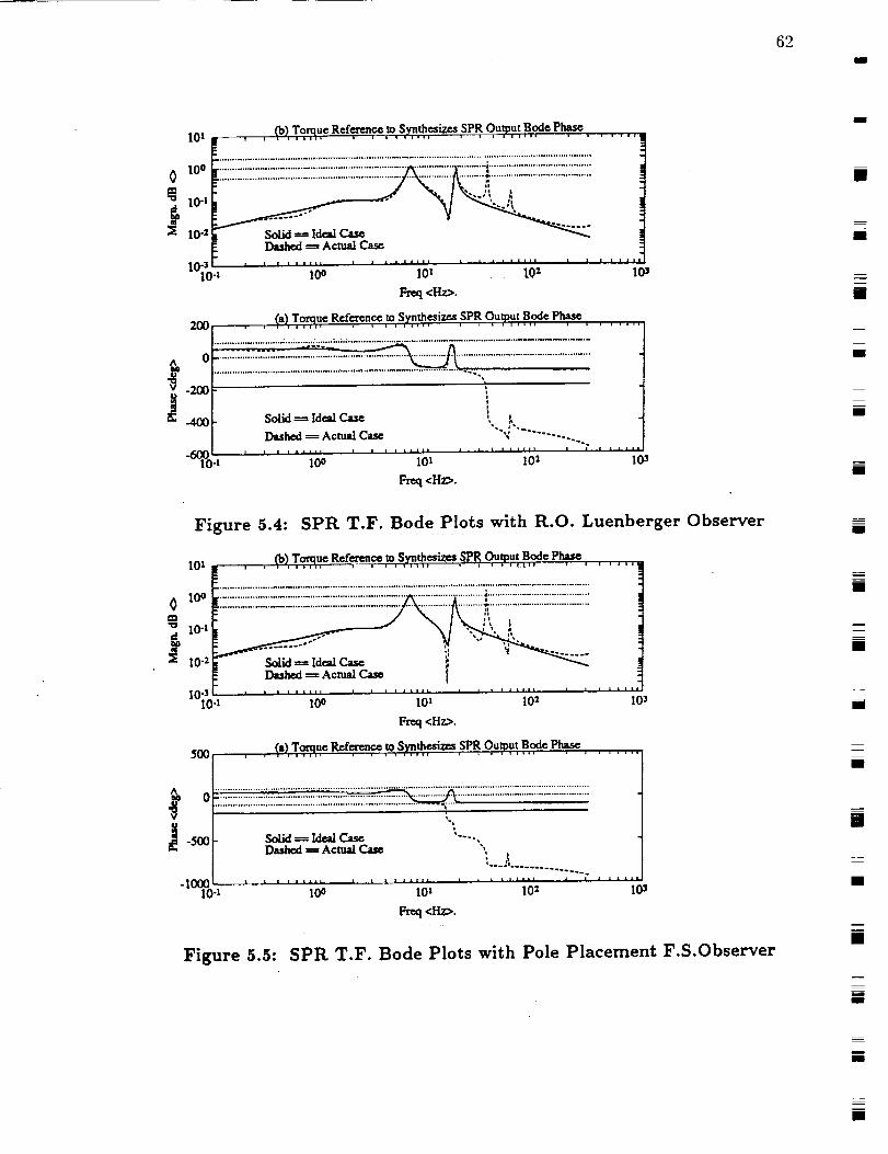
62mm

I01

0 10°

"= 10-t

i0.2

10-]lO-1

2OO

^ 0

"_ -200

-60010-1

Solid == Id,_1Ca_

Dashed ----ActualCs.sc, i r i ||llt I | i i 1_tJ i

10 o 101

Freq<Hz>.

(b) Toque Reference to Synthesizes SPR Output Bode Phase--_ l , I I l , I , t I 'l l l , , i , , T 1 111,91 . I , i , , i

.......... ' .......................................................................................... i .........................................

,..;,,

Dashed ----Acn_l

.................. 10 o 10' ' .............. 10 '_ I(P

r-rtq<Hz>.

(a) Torquc Reference to SFnthesizea SPR Output Bode Pha._, • | t ,,,_ , , , i ii,i, j i r i jl*l, i , , J , ,,,

-_.:.:...:-:.-._._.:.::.....7.'.-.'..'.'...__ 7777.........................................

102 103

Figure 5.4:

10 t

SPR T.F. Bode Plots with R.O. Luenberger Observer

(b) Torque Refe=ence to Synthesizes SPR Output Bode Phase, i i, ,,,,o ! ! i i liiJl i q D _ ,,_,| _ 6 , . . i,

, ..it

I0 3

0 Ioo ................................................................................._,.....................................m ;, ;

10.t , ,, •

10 "2 Solid -----Idcal Ca_---- Actual f

10"l().t 10 o 10 t 10 z

Fr_ <Hz>.

soo , . 9)T,'_,,u"R_f_,_,,o,s_,_ _sr_o,,,_ ,_,9"r,_, ,

-$00 Solid _ Idol _ '"

D_I ---- Actual Ca_e "'"',!

°--- ................ .

"?'o-, lOO 10' 102 10_

F_q <Hz>.

Figure 5.5: SPR T.F. Bode Plots with Pole Placement F.S.Observer

i

i

m

am

m

mm

am

==

am

m

m

i

m

[]

z

m

[]

mmi

*am

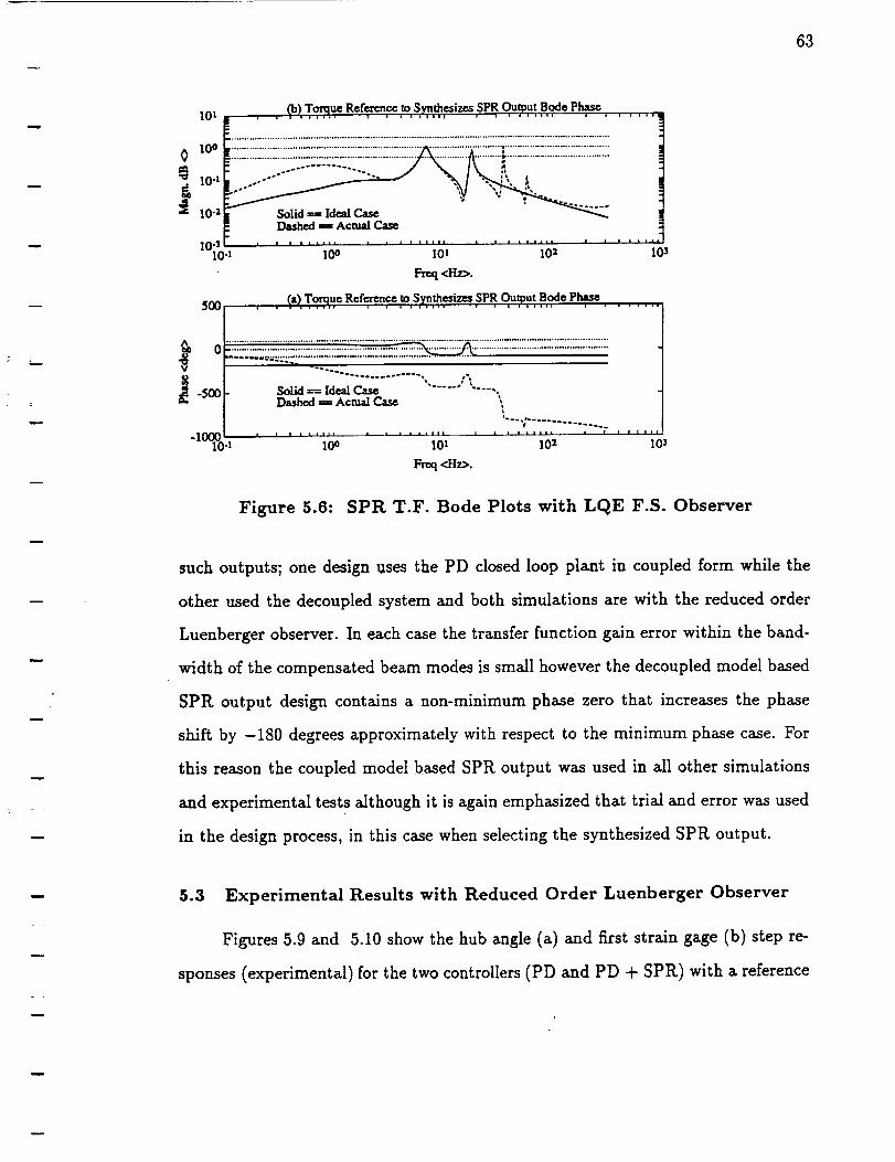
63

10 s

0 10°

-e 10. l

_10 4

10-310-I

_b) Torque Reference to Synthesizes SPR Output Bode Phase.

....................................................................................................... i .......................................

Solid == Idea/Case .........Dashed =_ Actual Case

J ] [ i ] I I I t i J [ i J i J i ] i i l i i i i i i [ i i i a i /

10o 101 102 103

_,q <Hz>.

_a)T,o_qu¢ Rcf,eren,ce ,to,S_. _,esizes SPR Ou,tput ,B,,ode P,h_ .......5OO

Ao

-500

-I000lO-I

Solid ---= Ideal CaseDashed _ Actual Case \

101 10 z 10 3

Freq <Hz_.

Figure 5.6: SPR T.F. Bode Plots with LQE F.S. Observer

such outputs; one design uses the PD closed loop plant in coupled form while the

other used the decoupled system and both simulations are with the reduced order

Luenberger observer. In each case the transfer function gain error within the band-

width of the compensated beam modes is small however the decoupled model based

SPR output design contains a non-minimum phase zero that increases the phase

shift by -180 degrees approximately with respect to the minimum phase case. For

this reason the coupled model based SPR output was used in all other simulations

and experimental tests although it is again emphasized that trial and error was used

in the design process, in this case when selecting the synthesized SPR output.

w

u

w

5.3 Experimental Results with Reduced Order Luenberger Observer

Figures 5.9 and 5.10 show the hub angle (a) and first strain gage (b) step re-

sponses (experimental) for the two controllers (PD and PD + SPR) with a reference

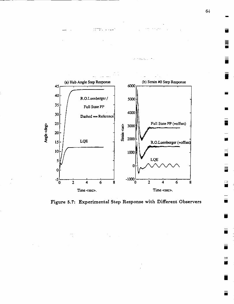
64

i

[]

i

[]

V

e_

45

4O

35

3O

25

2O

15

I0

5

0

-50

(a) Hub Angle Step Response

R.O.Luenberger/

FullState PP

Dashed ===Refercnc:

LQE

Time <sec>.

60OO(b)Swain #0 Step Response

i

500O

4O0O

-I000 " ' '0 2 4 6 8

Time <sec>.

Figure 5.7: Experimental Step Response with Different Observers

[]

z

m

m

i

i

ii

z

il

i

[]

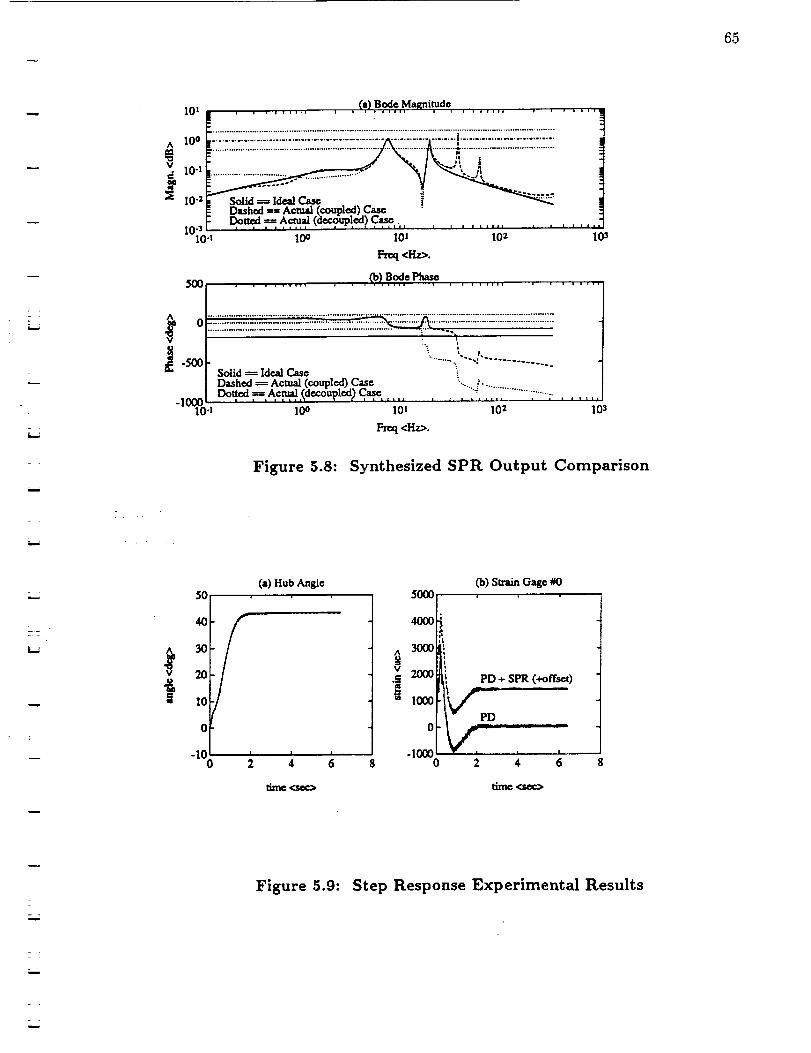
65

=

101

^ 10 °

v10 "1

lO-a

10-310-1

500

0

-500

(a) Bode Magnitude

......Solid _ Ideal Case ._ .... "_'"Dashed == Actual (coupled) Case.13ot_. _. ,A,_'_,, (decgn!ed I ,C_,,.,,

,oo lo, ...... io', ...... _o,F'nxl<Hz>.

.......... _,_,,s_,eP_ ........ _:. .....

-100010-1

•. , .... ..

Solid _ Ideal CaseDashed _ Actual (coupled) Case 'Do .ued _ Actual.` ,(decouplexi) C.,a_ ..... ""- ..............................

| j , i ,ll|l , t • . I It

10o 101 102 103

Freq <Hz>.

Figure 5.8: Synthesized SPR Output Comparison

i

5O

^ 30

0

"100

(a) Hub Angle

I I

4 6

time <sec>

5000

4000

1000

0

-1000

(b) Strain Gage #0

0 8

PD + SPR (+offset)

PD

2 4 6

Figure 5.9: Step Response Experimental Results

m

Z_

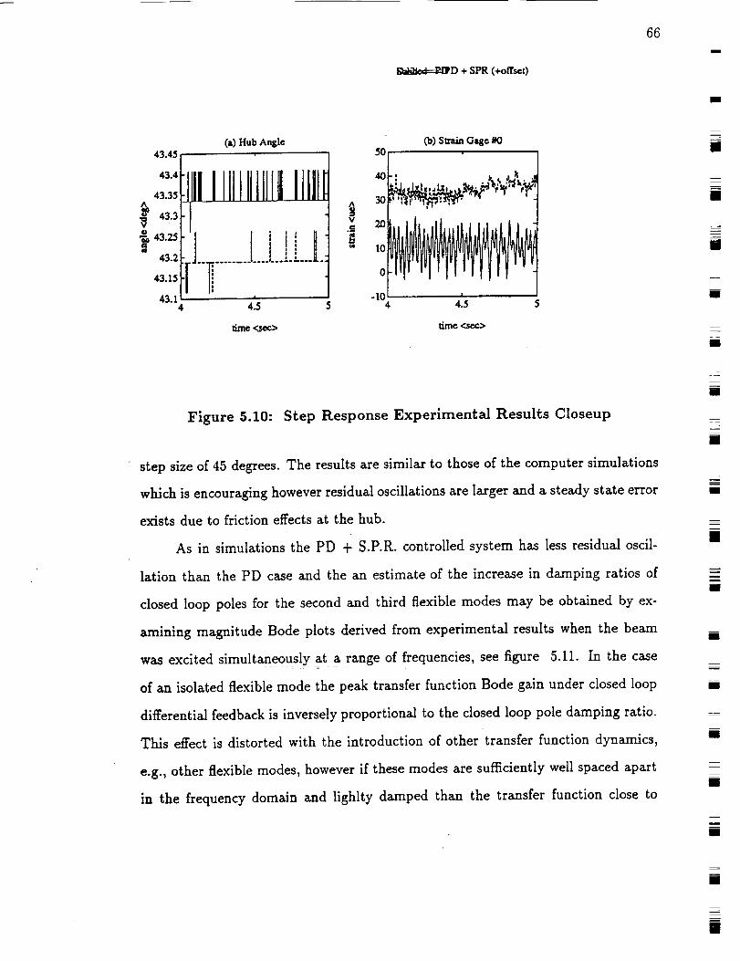
_D + SPR (+offsc0

66

m

43.45

43.4

43.33A

_ 43.3

U

43.25

43.2

43.15

43.14

(a) Hub Angl*t

J HJ....t.....-.A.

4.5

_-nc <scc>

Co)Strain Gage #050

40l i , _._ ,A..J

.ii.10 I

5 4 4..5 5

tirn¢ <se_>

J

Z

[]

I

BB

Figure 5.10: Step Response Experimental Results Closeup

step size of 45 degrees. The results are similar to those of the computer simulations

which is encouraging however residual oscillations are larger and a steady state error

exists due to friction effects at the hub.

As in simulations the PD + S.P.R. controlled system has less residual oscil-

lation than the PD case and the an estimate of the increase in damping ratios of

closed loop poles for the second and third flexible modes may be obtained by ex-

amining magnitude Bode plots derived from experimental results when the beam

was excited simultaneously at a range of frequencies, see figure 5.11. In the case

of an isolated flexible mode the peak transfer function Bode gain under closed loop

differential feedback is inversely proportional to the closed loop pole damping ratio.

This effect is distorted with the introduction of other transfer function dynamics,

e.g., other flexible modes, however if these modes are sufficiently well spaced apart

in the frequency domain and lighlty damped than the transfer function close to

I

[]

am

[]

i

zam

mm

m

mm

Im

[]

[]

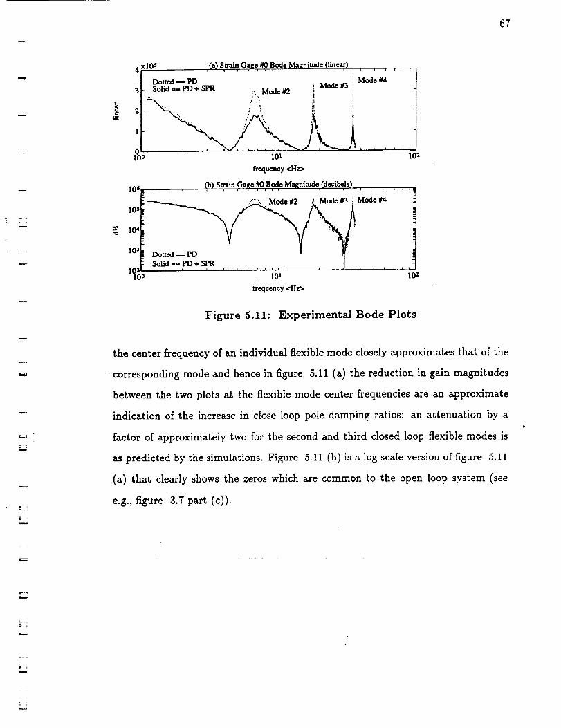
67

w

.E

4xl0S

3

2

1

010 o

106

105

104

103

10:10o

. {a) S m_. Gage _ Bode Magnitude (linear) , , ,

Dotted _--_ PD [ Mode #4

Solid =ffi PD + SPR :. Mode #2Mode #3 i

lot

frequency <Hz>

I t •

lOZ

_b)Swain.Gage#O,Bode Magnitude,(decibels)......

Dotted_ PD _

Solid _= PD + SPR [B

! I i ! ! ¢ i a i , .. l ; , ] _

101 10 2

frequency <Hz>

Figure 5.11: Experimental Bode Plots

the center frequency of an individual flexible mode closely approximates that of the

corresponding mode and hence in figure 5.11 (a) the reduction in gain magnitudes

between the two plots at the flexible mode center frequencies are an approximate

indication of the increase in close loop pole damping ratios: an attenuation by a

factor of approximately two for the second and third closed loop flexible modes is

as predicted by the simulations. Figure 5.11 (b) is a log scale version of figure 5.11

(a) that clearly shows the zeros which are common to the open loop system (see

e.g., figure 3.7 part (c)).

I

CONCLUSIONS

The hub angle PD compensator derived from the linear normal mode model produces

very good results in terms of the hub angle step response which has no overshoot

and little residual oscillation in both simulations and real tests The same is also

true for the beam tip displacement for the simulated case and although this cannot

yet be directly verified for the real testbed case low residual oscillations in the tip

displacement are implied by the low residual oscillations in the strain signals.

Adding a second SPR static gain full state feedback loop can improve the step

response performance further in a robust manner by increasing the flexible mode

pole damping ratios. Such compensation has a phase margin of at least [-90, 90]

degrees in the ideal case and this is found to be also true for simulations that

include observer effects and some unmodeled modes within the bandwidth of the

compensated modes though not at higher frequencies. This suggests the addition

of a low pass filter in the SPR feedback loop that maintains a low phase shift and

nearly constant gain in the compensated mode bandwidth in order to maintain the

low frequency closed loop performance already achieved, with a gain roll off at higher

frequencies to attenuate unwanted effects.

Of the three closed loop observers tested the two with poles placed above the

highest compensated mode center frequency produced the least distortion on the

synthesized SPR transfer function and the best experimental closed loop perfor-

mance.

The controller design procedure used appears basically sound and produced

good results however it is fractured and involved trial and error selections. The task

now is to synthesize these observer/compensator blocks either separately or together

in a systematic and optimum fashion.

68

m

U

I

!

m

z

I

m

m

i

I

[]

m

m

z

m

U

D

m

[]

w

LITERATURE CITED

b

r

[1] Feiyue Wang and John T. Wen. Nonlinear Dynamical Model and Control For

A Flexible Beam. CIRSSE Report No.75 Rensselaer Polytechnic Institute,

NY, Nov, 1990.

[2] John.T. Wen. Time Domain and Frequency Domain Conditions for Strict

Poistive Realness IEEE Transactions On Automatic Control, Vol. 33, No. 10,

October 1988.

[3] R.H. Cannon, Jr. and E.Schmitz. Precise control of flexible manipulators. In

M.Brady and R.Paul, editors, Robotics Research: The First International

Symposium, pages 841-861. MIT Press, Cambridge, MA, 1984.

[4] C. Desoer. Feedback Systems: Input-Output Properties. Academic Press,1975.

[5] Chi-Tsong Chen. Linear System Theory and Design. Holt, Rinehart and

Winston, Inc., Revised Version, 1984, ISBN 0-03-06-289-0

L

= •

w

69

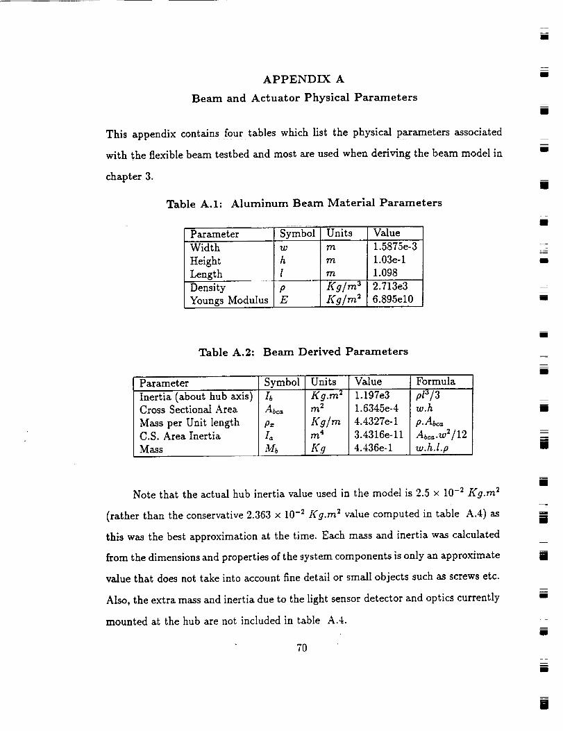
l

APPENDIX A

Beam and Actuator Physical Parameters

This appendix contains four tables which list the physical parameters associated

with the flexible beam testbed and most are used when deriving the beam model in

chapter 3.

Table A.I: Aluminum Beam Material Parameters

Parameter Symbol Units Value

Width w m 1.5875e-3

Height h m 1.03e-1

Length l m 1.098

Density p Kg/rn 3 2.713e3

Youngs Modulus E Kg/rn 2 6.895e10

l

88

I

z

I

I

I

Table A.2: Beam Derived Parameters

m

m

Parameter

Inertia (about hub axis)

Cross Sectional Area

Mass per Unit length

C.S. Area Inertia

Mass

Symbol

hAbea

IoMb

Units

K g.rn 2

rn 2

Kg/mm 4

Kg

Value

1.197e3

1.6345e-4

4.4327e-1

3.4316e-ll

4.436e-1

Formula

p13/3w.h

p.Abc,,

Abc,, .w2 /12

w.h.l.p

Z

I

g

Note that the actual hub inertia value used in the model is 2.5 x 10 -2 Kg.m 2

(rather than the conservative 2.363 x 10 -2 Kg.m 2 value computed in table A.4) as

this was the best approximation at the time. Each mass and inertia was calculated

from the dimensions and properties of the system components is only an approximate

value that does not take into account fine detail or small objects such as screws etc.

Also, the extra mass and inertia due to the light sensor detector and optics currently

mounted at the hub are not included in table A.4.

7O

mm

[]

m

I

m

l

71

i=i :

Table A.3: Motor Parameters

Parameter

Shaft Inertia

Shaft Mass

Torque Constant

Continuous Stall Torque

Peak Torque

Electrical Time Constant

Symbol

M._

KT

TS

TP

TE

Units

Kg.m 2

Kg

Nm/A

Nrn

Nrn

8ec

Value

1.201e-4

2.370e-1

1.2407

1.358el

1.4e-4

Table A.4: Hub Derived Parameters

w

v

Item

Symbol

Motor Shaft

Hub Collar

Encoder Collar

Bellows

Potentiometer

Hub Base

Hub Base Strengthener

Counter Weight

Counter Weight Bar

Balance weight Bar

Weight Bar Block

Beam Post

Mass

MhKg

4.798e-2

1.126

7.476e-1

4.123e-2

2.611e-2

3.619e-3

3.941e-1

Inertia

hKg.m 2

1.201e-4

3.869 e-6

6.707e-3

1.482e-2

7.047e-4

3.263e-4

3.000e-5

9.214e-4

Hub Assembly total 2.386 2.363e-2

#

1

1

1

1

1

1

1

1

1

2

3

2

n

i

i

i

i

i

u

me

i

i

i

i

i

i

m

a