Single Machine Scheduling: Comparison of MIP … Machine Scheduling: Comparison of MIP Formulations and ... number of tardy jobs for the two sets of jobs is studied. A ... of this

Single Machine Scheduling: Comparison of MIP Formulations and Heuristics for

Interfering Job Sets

by

Ketan Khowala

A Dissertation Presented in Partial Fulfillment of the Requirements for the Degree

Doctor of Philosophy

Approved December 2011 by the Graduate Supervisory Committee:

John Fowler, Co-Chair Ahmet Keha, Co-Chair

Hari Jagannathan Balasubramanian Teresa (Tong) Wu

Muhong Zhang

ARIZONA STATE UNIVERSITY

May 2012

i

ABSTRACT

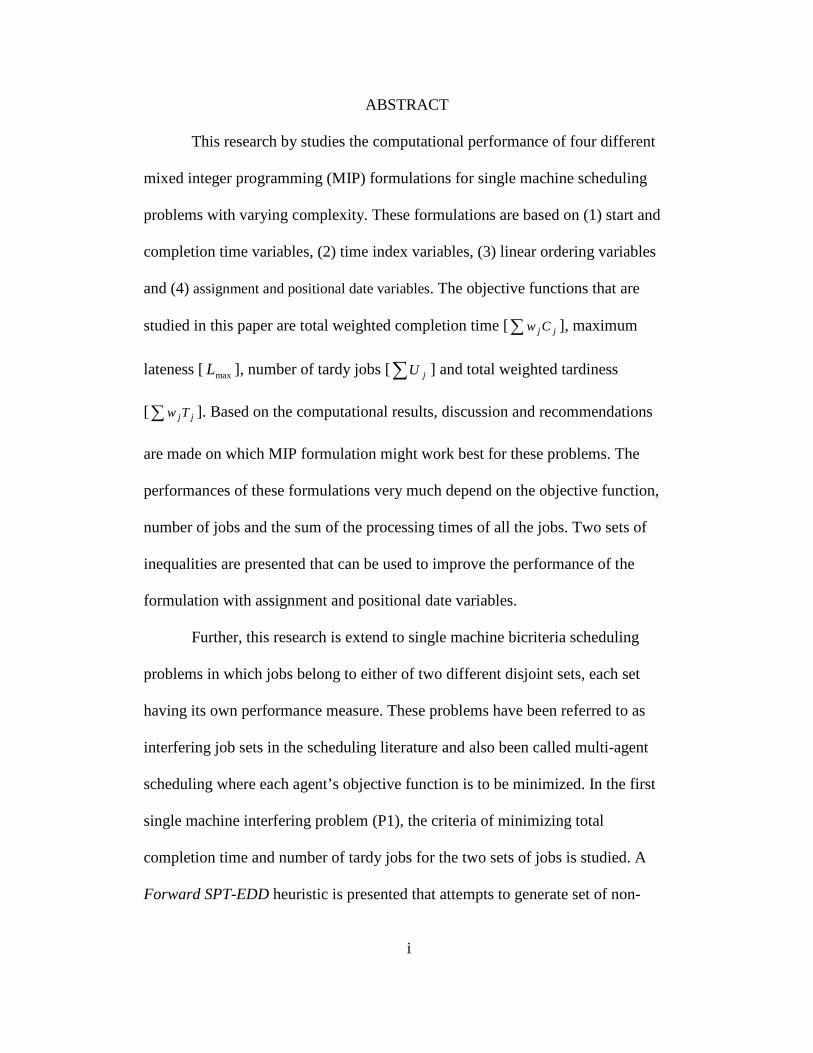
This research by studies the computational performance of four different

mixed integer programming (MIP) formulations for single machine scheduling

problems with varying complexity. These formulations are based on (1) start and

completion time variables, (2) time index variables, (3) linear ordering variables

and (4) assignment and positional date variables. The objective functions that are

studied in this paper are total weighted completion time [ jj Cw∑ ], maximum

lateness [ maxL ], number of tardy jobs [∑ jU ] and total weighted tardiness

[ jj Tw∑ ]. Based on the computational results, discussion and recommendations

are made on which MIP formulation might work best for these problems. The

performances of these formulations very much depend on the objective function,

number of jobs and the sum of the processing times of all the jobs. Two sets of

inequalities are presented that can be used to improve the performance of the

formulation with assignment and positional date variables.

Further, this research is extend to single machine bicriteria scheduling

problems in which jobs belong to either of two different disjoint sets, each set

having its own performance measure. These problems have been referred to as

interfering job sets in the scheduling literature and also been called multi-agent

scheduling where each agent’s objective function is to be minimized. In the first

single machine interfering problem (P1), the criteria of minimizing total

completion time and number of tardy jobs for the two sets of jobs is studied. A

Forward SPT-EDD heuristic is presented that attempts to generate set of non-

ii

dominated solutions. The complexity of this specific problem is NP-hard. The

computational efficiency of the heuristic is compared against the pseudo-

polynomial algorithm proposed by Ng et al. [2006]. In the second single machine

interfering job sets problem (P2), the criteria of minimizing total weighted

completion time and maximum lateness is studied. This is an established NP-hard

problem for which a Forward WSPT-EDD heuristic is presented that attempts to

generate set of supported points and the solution quality is compared with MIP

formulations. For both of these problems, all jobs are available at time zero and

the jobs are not allowed to be preempted.

iii

Dedicated to Awakash

iv

ACKNOWLEDGMENTS

I would like to express my gratitude to my committee co-chairs Dr. John W.

Fowler and Dr. Ahmet Keha and to my committee members Dr. Hari J.

Balasubramanian, Dr. Teresa Wu and Dr. Muhong Zhang, for their valuable

guidance and support in completing this research. I would like to thank Dr.

Fowler especially for being a mentor for over ten years and providing me various

research and learning opportunities at Arizona State University. Thanks are due to

all my family, friends and lab mates for their encouragement and support.

v

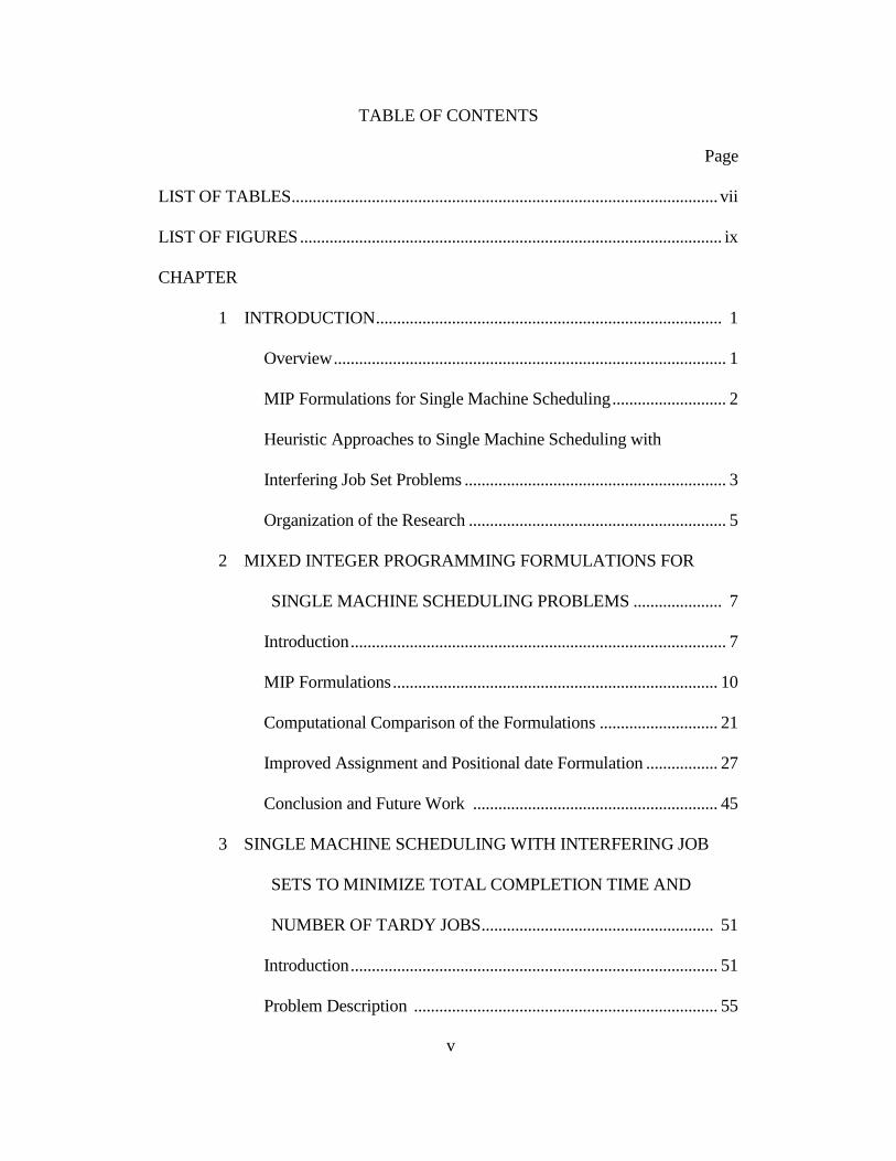
TABLE OF CONTENTS

Page

LIST OF TABLES ..................................................................................................... vii

LIST OF FIGURES .................................................................................................... ix

CHAPTER

1 INTRODUCTION .................................................................................. 1

Overview ............................................................................................. 1

MIP Formulations for Single Machine Scheduling ........................... 2

Heuristic Approaches to Single Machine Scheduling with

Interfering Job Set Problems .............................................................. 3

Organization of the Research ............................................................. 5

2 MIXED INTEGER PROGRAMMING FORMULATIONS FOR

SINGLE MACHINE SCHEDULING PROBLEMS ..................... 7

Introduction ......................................................................................... 7

MIP Formulations ............................................................................. 10

Computational Comparison of the Formulations ............................ 21

Improved Assignment and Positional date Formulation ................. 27

Conclusion and Future Work .......................................................... 45

3 SINGLE MACHINE SCHEDULING WITH INTERFERING JOB

SETS TO MINIMIZE TOTAL COMPLETION TIME AND

NUMBER OF TARDY JOBS ....................................................... 51

Introduction ....................................................................................... 51

Problem Description ........................................................................ 55

vi

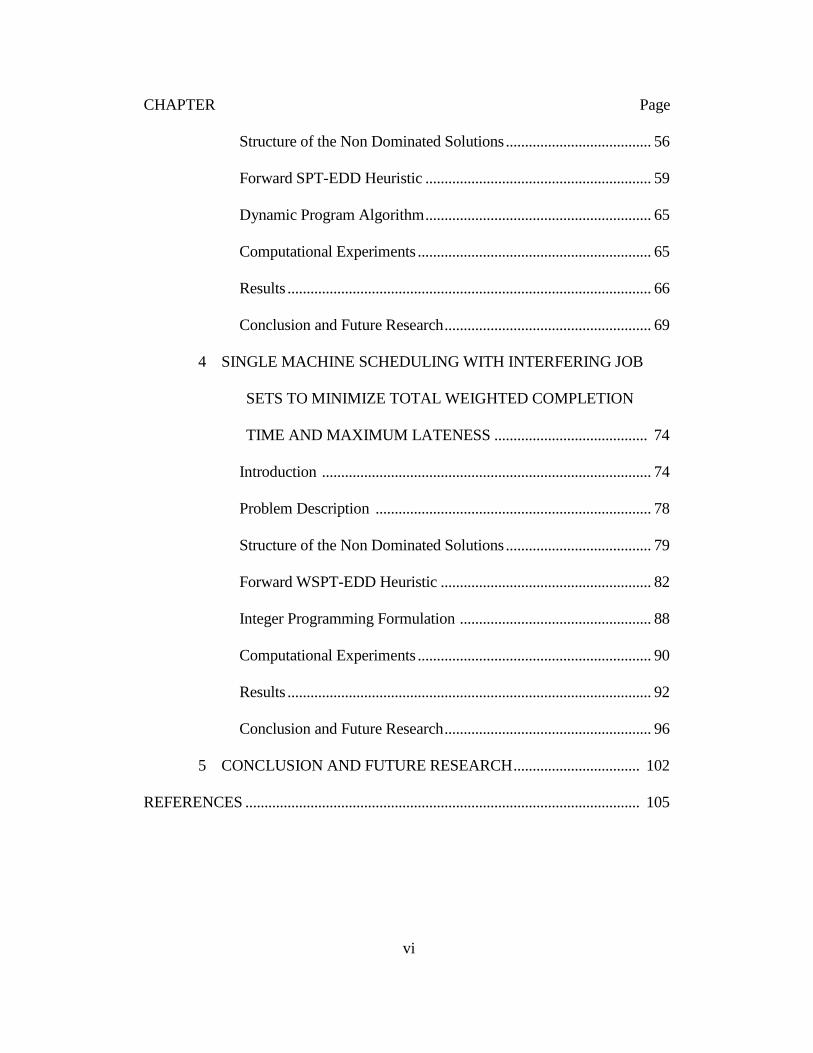
CHAPTER Page

Structure of the Non Dominated Solutions ...................................... 56

Forward SPT-EDD Heuristic ........................................................... 59

Dynamic Program Algorithm ........................................................... 65

Computational Experiments ............................................................. 65

Results ............................................................................................... 66

Conclusion and Future Research ...................................................... 69

4 SINGLE MACHINE SCHEDULING WITH INTERFERING JOB

SETS TO MINIMIZE TOTAL WEIGHTED COMPLETION

TIME AND MAXIMUM LATENESS ........................................ 74

Introduction ...................................................................................... 74

Problem Description ........................................................................ 78

Structure of the Non Dominated Solutions ...................................... 79

Forward WSPT-EDD Heuristic ....................................................... 82

Integer Programming Formulation .................................................. 88

Computational Experiments ............................................................. 90

Results ............................................................................................... 92

Conclusion and Future Research ...................................................... 96

5 CONCLUSION AND FUTURE RESEARCH ................................. 102

REFERENCES ....................................................................................................... 105

vii

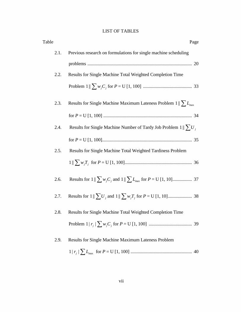
LIST OF TABLES

Table Page

2.1. Previous research on formulations for single machine scheduling

problems ............................................................................................ 20

2.2. Results for Single Machine Total Weighted Completion Time

Problem ∑ jjCw||1 for P = U [1, 100] ........................................... 33

2.3. Results for Single Machine Maximum Lateness Problem ∑ max||1 L

for P = U [1, 100] .............................................................................. 34

2.4. Results for Single Machine Number of Tardy Job Problem ∑ jU||1

for P = U [1, 100]............................................................................... 35

2.5. Results for Single Machine Total Weighted Tardiness Problem

∑ jjTw||1 for P = U [1, 100] ........................................................... 36

2.6. Results for ∑ jjCw||1 and ∑ max||1 L for P = U [1, 10] ................. 37

2.7. Results for ∑ jU||1 and ∑ jjTw||1 for P = U [1, 10] ..................... 38

2.8. Results for Single Machine Total Weighted Completion Time

Problem ∑ jjj Cwr ||1 for P = U [1, 100] ...................................... 39

2.9. Results for Single Machine Maximum Lateness Problem

∑ max||1 Lr j for P = U [1, 100] ...................................................... 40

viii

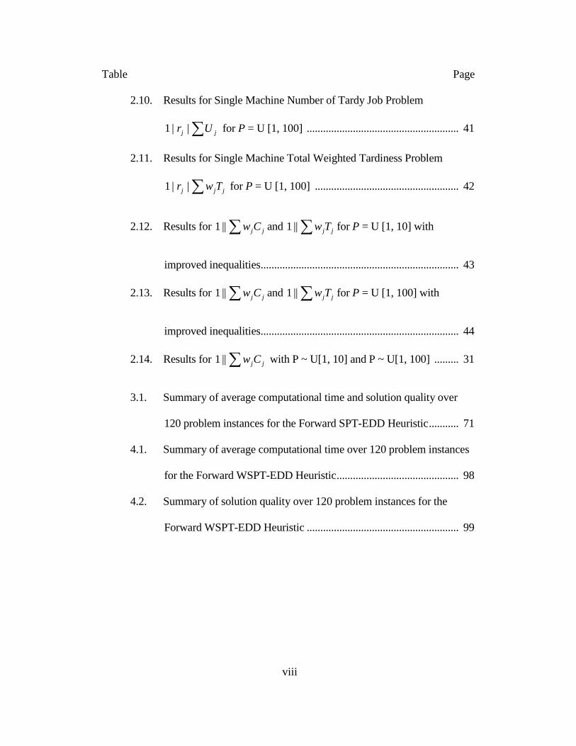
Table Page

2.10. Results for Single Machine Number of Tardy Job Problem

∑ jj Ur ||1 for P = U [1, 100] ........................................................ 41

2.11. Results for Single Machine Total Weighted Tardiness Problem

∑ jjj Twr ||1 for P = U [1, 100] ..................................................... 42

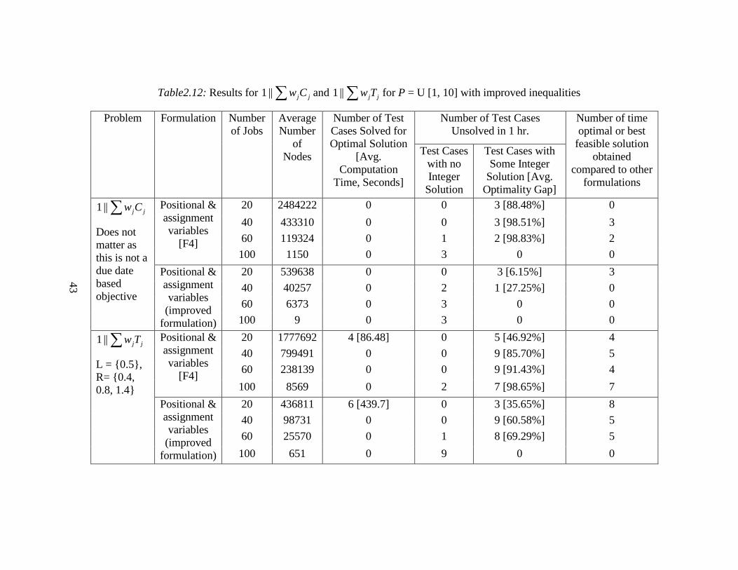
2.12. Results for ∑ jjCw||1 and ∑ jjTw||1 for P = U [1, 10] with

improved inequalities......................................................................... 43

2.13. Results for ∑ jjCw||1 and ∑ jjTw||1 for P = U [1, 100] with

improved inequalities......................................................................... 44

2.14. Results for ∑ jjCw||1 with P ~ U[1, 10] and P ~ U[1, 100] ......... 31

3.1. Summary of average computational time and solution quality over

120 problem instances for the Forward SPT-EDD Heuristic ........... 71

4.1. Summary of average computational time over 120 problem instances

for the Forward WSPT-EDD Heuristic ............................................. 98

4.2. Summary of solution quality over 120 problem instances for the

Forward WSPT-EDD Heuristic ........................................................ 99

ix

LIST OF FIGURES

Figure Page

3.1. Structure of non dominated points with total completion time and

number tardy jobs as performance criteria ........................................ 58

3.2. Efficient frontier representing non dominated points for job in

set 1ξ and 2ξ ........................................................................................ 58

3.3a. In the first step jobs in 1S are allowed to be preempted. In the second

step jobs in set 2S are moved ahead to avoid preemption of jobs in

set 1S . Note that the completion time of the jobs in 1S remains the

same .................................................................................................... 63

3.3b. In the first step job #2 from set 2S is moved to 3S and jobs in set 1S are

allowed to be preempted. In the second step jobs in set 2S are moved

ahead to avoid preemption of jobs in set1S . Note that the completion

time of the jobs in 1S remains the same ............................................. 63

3.3c. In the first step job #1 from set 2S is moved to 3S and jobs in set 1S are

allowed to be preempted. In the second step jobs in set 2S are moved

ahead to avoid preemption of jobs in set1S . Note that the completion

time of the jobs in 1S remains the same ............................................. 64

3.3d. Job #3 from set 2S is moved to 3S and jobs in set 1S are already in a

non preemptive SPT order ................................................................ 64

3.4. Average run time across 20 problem instances for Forward SPT-EDD

heuristic as well as for the Dynamic Program .................................. 67

x

Figure Page

4.1. Structure of non dominated points with total weighted completion

time and maximum lateness as performance criteria ........................ 81

4.2. Efficient frontier representing non dominated points for job in

set 1ξ and 2ξ ......................................................................................... 81

4.3a. In the first row jobs in 1ξ are allowed to be preempted. In the second

row jobs in set 2ξ are pulled ahead to avoid preemption of jobs in

set 1ξ which creates a non-preemptive and feasible schedule. Note that

the completion time of the jobs in 1ξ remains the same ................... 86

4.3b. In the first row, all the jobs from set 2ξ are moved by one time unit

and jobs in set 1ξ are allowed to be preempted. In the second row jobs

in set 2ξ are pulled ahead to avoid preemption of jobs in set1ξ , which

creates a non-preemptive and feasible schedule ............................... 87

4.3c. In the first row, all the jobs from set 2ξ are moved by another one time

unit and jobs in set 1ξ are allowed to be preempted. In the second row

jobs in set 2ξ are pulled ahead to avoid preemption of jobs in set1ξ ,

which creates a non-preemptive and feasible schedule .................... 87

4.3d. This is the last iteration, where all the jobs in set1ξ are placed in the

beginning of the schedule, thus providing the best possible objective

value for set1ξ .................................................................................... 88

1

Chapter 1

INTRODUCTION

1. Overview

Scheduling is motivated by questions that arise in production planning, in

balancing processes sent to compute nodes, in telecommunications and generally

in all situations in which scarce resources have to be allocated to activities over

time. Although finding a feasible solution to a scheduling problem is often easy, it

is usually nontrivial to find an optimal or near optimal solution to a scheduling

problem. In this paper we approach scheduling problems from the point of view

of a practitioner who does not have expertise in scheduling and integer

programming. Formulating a problem as a mixed integer program (MIP) and

using the default settings of one of the commercially available software to solve

this model is the first thing that a practitioner without an expertise in scheduling

would do instead of using problem specific branch and bound algorithms. Further,

when the problems are more complex in nature (such as bicriteria problem or

problems of interfering job sets), a practitioner might want resort to good heuristic

solutions. Therefore this paper is focused on solving scheduling problems using

mixed integer programming formulations as well as simple heuristics which

exploit the structure of the problem.

2

2. MIP Formulations for Single Machine Scheduling

In the first step we compare the computational performance of different

mixed integer programming (MIP) formulations for different single machine

scheduling problems. The MIP formulations for scheduling problems are often

classified based on the choice of the decision variables. The different decision

variables used to distinguish four different MIP formulations in this research are

(i) completion time variables [Balas (1985)] (ii) time index variables [Sousa and

Wolsey (1992)] (iii) linear ordering variables [Dyer and Wolsey (1990)] and (iv)

assignment and positional date variables [Lasserre and Queyranne (1992)].

Queyranne and Schulz (1994) give a comprehensive survey of these MIP

formulations. We complement this paper by comparing the computational

performances of these formulations.

The objective functions that are studied are total weighted completion time

[ jj Cw∑ ], maximum lateness [maxL ], number of tardy jobs [∑ jU ] and total

weighted tardiness [ jj Tw∑ ]. These problems are studied with and without release

date constraints. Three out of the eight single machine problems that we study are

solvable in polynomial time by well known algorithms: WSPT (weighted shortest

processing time first) for total weighted competition time [Smith (1956)], EDD

(earliest due date) for maximum lateness [Jackson (1955)] and Moore’s algorithm

for number of tardy jobs [Moore (1968)]. However with release date constraints,

these problems become NP-hard [Lenstra et al. (1977), Kise et al. (1978)]. Total

3

weighted tardiness problem is NP-hard with and without release dates [Lawler

(1977)]. We wanted to get a wider understanding of the computational

efficiencies and behavior of different MIP formulations and therefore we also

considered some easy problems as well as the harder problems.

Based on the computational results, we discuss which MIP formulation

might work best for these problems. The performance of these formulations very

much depend on the objective function, number of jobs and the sum of the

processing times of all the jobs. We also present two sets of inequalities that can

be used to improve the formulation with assignment and positional date variables.

3. Heuristic Approaches to Single Machine Scheduling with Interfering Job Set

Problems

Motivated by multiple objectives and trade off that a decision maker has to

make between conflicting objectives, multicriteria scheduling problems have been

widely dealt with in the literature [T’Kindt et al (2006)]. Typically in these

scheduling problems one has to satisfy multiple criteria on the same set of jobs.

Little work has been done in the area of scheduling jobs where jobs belong to

different job sets and have to be processed using the same resource (or competing

for the same machine), hence causing interference. These job sets can have

different criteria to be minimized. These different sets may represent different

customers or agents whose requirements may differ.

4

The complexity of this domain of problems can be attributed to the

number of different job sets considered, the specific performance criteria

considered, restrictions on each set of jobs; and the machine environment. This is

a relatively new research area in scheduling where some of the work done earlier

has classified some of these problems as solvable in polynomial time, some as

strongly NP hard and some for which the complexity is yet not determined. Also

there is a wide range of problems in this domain which have not been considered.

The paper from Baker and Smith [2003] was the first paper formalizing

scheduling problems with interfering job sets. Using MIP formulations for this

domain of problems could be difficult as well as computationally challenging. We

look at some of these problems and exploit their structure to define heuristics

which yields near optimal solutions without many computational challenges.

In the first single machine interfering problem (P1) we look at minimizing

total completion time and number of tardy jobs for the two sets of jobs and

present a Forward SPT-EDD heuristic that attempts to generate set of non-

dominated solutions. The complexity of this specific problem is NP-hard. The

computational efficiency of the heuristic is compared against the pseudo-

polynomial algorithm proposed by Ng et al. [2006]. In the second single machine

interfering problem (P2) we look at minimizing total weighted completion time

and maximum lateness. This is an established NP-hard problem for which we

propose a Forward WSPT-EDD heuristic that attempts to generate set of

supported points and compare our solution quality with MIP formulations. For

5

both of these problems, we assume that all jobs are available at time zero and the

jobs are not allowed to be preempted. Results of how these heuristics perform

compared to the optimal solutions (as well as difference in the computational

times) are presented in the subsequent chapters.

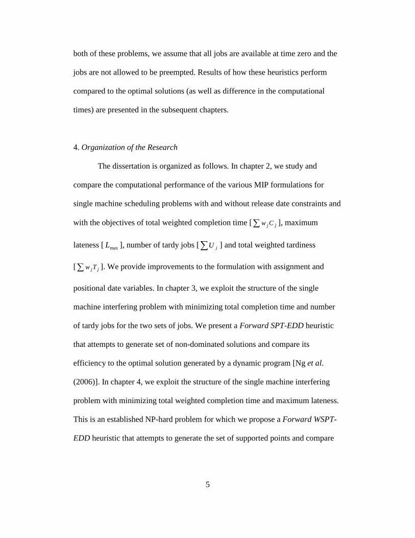
4. Organization of the Research

The dissertation is organized as follows. In chapter 2, we study and

compare the computational performance of the various MIP formulations for

single machine scheduling problems with and without release date constraints and

with the objectives of total weighted completion time [ jj Cw∑ ], maximum

lateness [ maxL ], number of tardy jobs [∑ jU ] and total weighted tardiness

[ jj Tw∑ ]. We provide improvements to the formulation with assignment and

positional date variables. In chapter 3, we exploit the structure of the single

machine interfering problem with minimizing total completion time and number

of tardy jobs for the two sets of jobs. We present a Forward SPT-EDD heuristic

that attempts to generate set of non-dominated solutions and compare its

efficiency to the optimal solution generated by a dynamic program [Ng et al.

(2006)]. In chapter 4, we exploit the structure of the single machine interfering

problem with minimizing total weighted completion time and maximum lateness.

This is an established NP-hard problem for which we propose a Forward WSPT-

EDD heuristic that attempts to generate the set of supported points and compare

6

our solution quality with MIP formulations. In chapter 5, we summarize the major

findings of the dissertation and list some of the future research areas.

7

Chapter 2

MIXED INTEGER PROGRAMMING FORMULATIONS FOR SINGLE

MACHINE SCHEDULING PROBLEMS

Abstract

In this paper, the computational performance of four different mixed integer

programming (MIP) formulations for various single machine scheduling problems

is studied. Based on the computational results, we discuss which MIP formulation

might work best for these problems. The results also reveal that for certain

problems a less frequently used MIP formulation is computationally more

efficient in practice than commonly used MIP formulations. We further present

two sets of inequalities that can be used to improve the formulation with

assignment and positional date variables.

Keywords: single machine scheduling, mixed integer programming, valid

inequalities

1. Introduction

Scheduling is motivated by questions that arise in production planning, in

balancing processes sent to compute nodes, in telecommunication and generally

in all situations in which scarce resources have to be allocated to activities over

time. Although finding a feasible solution to a scheduling problem is often easy, it

is usually nontrivial to find an optimal solution to a scheduling problem. In this

8

paper we approach scheduling problems from the point of view of a practitioner

who does not have expertise in scheduling and integer programming. Formulating

a problem as a mixed integer program (MIP) and using the default settings of one

of the commercially available software to solve this model is the first thing that a

practitioner without an expertise in scheduling would do instead of using problem

specific algorithms. Therefore this paper is focused on solving scheduling

problems using mixed integer programming formulations.

In this paper we compare the computational performance of different

mixed integer programming (MIP) formulations for different single machine

scheduling problems. The MIP formulations for scheduling problems are often

classified based on the choice of the decision variables. The different decision

variables used to distinguish four different MIP formulations in this paper are (i)

completion time variables [Balas (1985)] (ii) time index variables [Sousa and

Wolsey (1992)] (iii) linear ordering variables [Dyer and Wolsey (1990)] and (iv)

assignment and positional date variables [Lasserre and Queyranne (1992)].

Queyranne and Schulz (1994) give a comprehensive survey of these MIP

formulations. We complement this paper by comparing the computational

performances of these formulations.

9

We study various single machine problems, where n jobs are processed

through one machine and there is no preemption allowed while processing the

jobs. Let jp , jd , jw , jr , jC and jS be the processing time, due date, weight,

release date, completion time and start time of job j, respectively. We define

},....,2,1{ nN∈ as the set of the jobs. The lateness of job j, Lj, is defined

as jjj dCL −= and the tardiness of job j, Tj, is defined as }0,max{ jjj dCT −= . A

binary variable jU is defined to count the number of tardy jobs such that jU is

equal to 1 if job j is tardy, i.e. jC > jd and 0 otherwise. The objective functions

that are studied in this paper are total weighted completion time [∑ jj Cw ],

maximum lateness [maxL ], number of tardy jobs [∑ jU ] and total weighted

tardiness [∑ jjTw ]. In the scheduling notation of Graham et al. (1979), the

problems studied in this paper are denoted as∑ jjCw||1 , ∑ max||1 L , ∑ jU||1 ,

∑ jjTw||1 , ∑ jjj Cwr ||1 , ∑ max||1 Lr j , ∑ jj Ur ||1 and ∑ jjj Twr ||1 .

Three out of the eight single machine problems that we study are solvable

in polynomial time by well known algorithms: WSPT (weighted shortest

processing time first) for total weighted competition time [Smith (1956)], EDD

(earliest due date) for maximum lateness [Jackson (1955)] and Moore’s algorithm

for number of tardy jobs [Moore (1968)]. However with the release date

constraints, these problems become NP-hard [Lenstra et al. (1977), Kise et al.

10

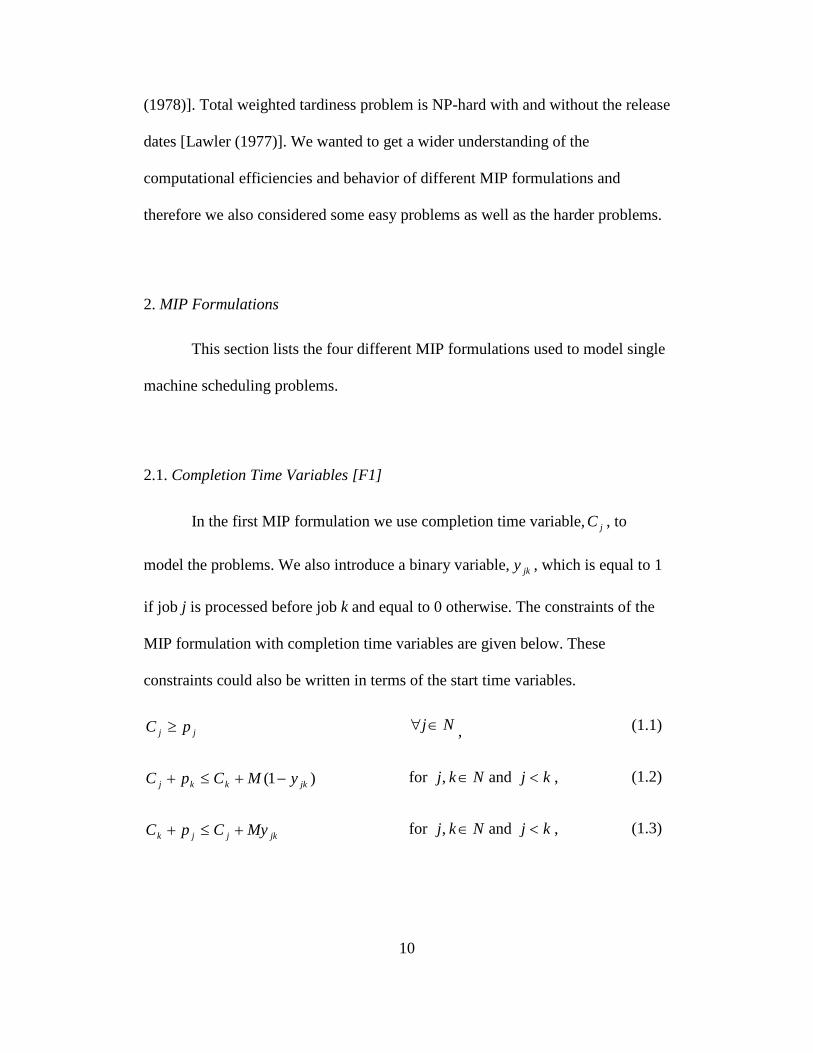
(1978)]. Total weighted tardiness problem is NP-hard with and without the release

dates [Lawler (1977)]. We wanted to get a wider understanding of the

computational efficiencies and behavior of different MIP formulations and

therefore we also considered some easy problems as well as the harder problems.

2. MIP Formulations

This section lists the four different MIP formulations used to model single

machine scheduling problems.

2.1. Completion Time Variables [F1]

In the first MIP formulation we use completion time variable, jC , to

model the problems. We also introduce a binary variable, jky , which is equal to 1

if job j is processed before job k and equal to 0 otherwise. The constraints of the

MIP formulation with completion time variables are given below. These

constraints could also be written in terms of the start time variables.

jj pC ≥ Nj∈∀ , (1.1)

)1( jkkkj yMCpC −+≤+ for Nkj ∈ , and kj < , (1.2)

jkjjk MyCpC +≤+ for Nkj ∈ , and kj < , (1.3)

11

0≥jC Nj∈∀ , (1.4)

}1,0{∈jky Nkj ∈∀ , and kj < . (1.5)

Constraint set (1.1) ensures that the completion time of each job is greater

than or equal to its processing time. Constraint sets (1.2) and (1.3) are disjunctive

constraints which enforce that either job j is processed before job k or job k is

processed before job j for any pair of jobs. Further, constraint sets (1.4) and (1.5)

are the non-negativity and integrality constraints. In this formulation, the value of

big M is generally taken to be equal to the sum of the processing times of all jobs.

For the problems with release dates, the value of M is taken to be greater than the

sum of processing time of all the jobs and the maximum value of the release date

for all the jobs.

The objective function for minimizing the total weighted completion time

can be written as∑ =

n

j jj Cw1

. The problem of minimizing the maximum lateness

can be modeled by minimizing LMAX as the objective function and adding the

following constraints to (1.1) – (1.5):

)( jj dCLMAX −≥ .Nj ∈∀ (1.6)

12

The problem of minimizing the number of tardy jobs is formulated by

minimizing ∑ =

n

j jU1

as the objective function and adding the following

constraints to (1.1) – (1.5):

jjj MUdC +≤ ,j N∀ ∈ (1.7)

}1,0{∈jU .Nj ∈∀ (1.8)

The problem of minimizing the total weighted tardiness is formulated by

minimizing the ∑ =

n

j jjTw1

as the objective function and adding the following

constraints to (1.1) – (1.5):

jjj dCT −≥ ,j N∀ ∈ (1.9)

0≥jT .Nj ∈∀ (1.10)

To complete the formulation using completion time variables for the

problems with the release date constraints, the equation (1.1) is replaced by

jjj rpC +≥ .Nj ∈∀ (1.11)

13

Balas (1985) presented the first work on formulating scheduling problems

using disjunctive constraints. This MIP formulation is also studied by Queyranne

and Wang (1991) and Queyranne (1993).

2.2. Time Index Variables [F2]

In the time index variables formulation, the planning horizon is

discretized into the periods 1, 2, 3, … T, where period t starts at time t-1 and ends

at time t. We introduce a binary time index variable,jtx , which is equal to 1 if job

j starts at time t and is equal to 0 otherwise. The constraints of the MIP

formulation with time index variables are as follows:

∑+−

=

=1

1

1jpT

tjtx ,j N∀ ∈ (2.1)

∑ ∑= +−=

≤n

j

t

ptsjs

j

x1 )1,0max(

1 Tt ,........,1= , (2.2)

}1,0{∈jtx

TtNj ,......,1; =∈∀ . (2.3)

The first constraint set (2.1) enforces that each job can start only at exactly

one particular time and the second constraint set (2.2) ensures that at any given

time at most one job can be processed. Constraint set (2.3) states the integrality

restriction. T assumes a value greater than the sum of processing times of all the

jobs. For the problems with release dates, T assumes a value greater than the sum

14

of processing time of all the jobs and the maximum value of the release date for

all the jobs. Using the time index variables, the completion time of a job j can be

written as

)1(1

1∑

+−

=

+−=jpT

tjtjj xptC

.Nj ∈∀ (2.4)

The objective function is

minimize∑ ∑=

+−

=

n

j jt

pT

tjt x

j

1

1

1

ξ

where

)1( jjjt ptw +−=ξ , 1,......, ,j N t T∀ ∈ = (2.5)

if we are minimizing the total weighted completion time;

1, ( 1),

0, otherwise, j j

jt

if t d pξ

> − +=

, 1,......, ,j N t T∀ ∈ = (2.6)

if we are minimizing the number of tardy jobs; and

]1 0, [ max jjjjt dptw −+−=ξ , 1,......, ,j N t T∀ ∈ = (2.7)

if we are minimizing the total weighted tardiness. Note that for all these problems

we don’t need any additional variables or constraints.

15

The problem of minimizing the maximum lateness can be modeled by

minimizing LMAX as the objective function and adding the constraint (1.6) by

substituting jC from (2.4).

To complete the formulation using time index variables for the problems

with the release date constraints, we set 0=jtx for jrt ≤ , .Nj ∈∀

Time index variables formulation was introduced by Sousa and Wolsey

(1992) for non-preemptive single machine scheduling problems. van den Akker et

al. (1999) and Šorić (2000) later studied this formulation for different machine

settings and objective functions.

2.3. Linear Ordering Variables [F3]

This formulation is based on binary linear ordering variables, jkδ , which

are equal to 1 when job j precedes job k and equal to 0, otherwise. The constraints

of the MIP formulation with linear ordering variables are as follows:

1=+ kjjk δδ nkj ≤≤≤1 , (3.1)

2≤++ ljkljk δδδ , , and j k l N j k l∈ ≠ ≠ , (3.2)

}1 ,0{∈jkδ ., Nkj ∈∀ (3.3)

16

Constraint set (3.1) is a set of conflict constraints, which ensure that either

job j is processed before job k or job k is processed before job j. Constraint set

(3.2) represents the transitivity constraints that ensure a linear order between three

jobs. Constraint set (3.3) states the integrality restriction. Using linear ordering

variables, the completion time of job j can be written as shown in constraint set

(3.4) and holds only if all the release dates are equal to zero.

j

jkNk

kjkj ppC +=∑≠∈

δ . .Nj ∈∀ (3.4)

The objective function for minimizing the total weighted completion time

can be written as ∑∑∈

≠∈

+Nj

jj

jkNkj

kjkj pwpw,

δ . The MIP formulations for the other

three objectives can be obtained by substituting jC from (3.4) into the constraints

(1.6), (1.7) and (1.9), and adding them to (3.1) – (3.3).

To formulate the problems with release date constraints using linear

ordering variables, we arrange the jobs in non increasing order of the release dates

and add the following constraints (3.5 and 3.6) (Nemhauser and Savelsbergh,

1992 can be referred for extra details).

∑ ∑≠< ≠≥

+−++≥jkik jkik

kjkkjikkijij pprS, ,

)1( δδδδ , ,i j N∀ ∈ (3.5)

1=jjδ , .Nj ∈∀ (3.6)

17

Further to formulate the various objective functions:∑ jj Cw , maxL , ∑ jU

and ∑ jjTw with release date constraint, the term ∑≠∈

jkNk

kjkp δ is replaced by jS

from the objective function and the inequalities.

The linear ordering formulation was first introduced by Dyer and Wolsey

(1990). It was later studied by Blazewicz et al. (1991), Nemhauser and

Savelsbergh (1992) and Chudak and Hochbaum (1999).

2.4. Assignment and Positional Date Variables [F4]

In this formulation, we define binary assignment variables,jku , which are

equal to 1 if job j is assigned to position k and are equal to 0 otherwise. Further,

we introduce positional date variables,kγ , which define the completion time of

the job at position k. The constraints of the MIP formulation with assignment and

positional date variables are as follows:

∑∈

=Nk

jku 1 Nj∈∀ , (4.1)

∑∈

=Nj

jku 1 Nk∈∀ , (4.2)

∑≥j

jj up 11γ (4.3)

∑+≥ −j

jkjkk up1γγ Nk ,.....,2= , (4.4)

18

0≥kγ Nk∈∀ , (4.5)

}1,0{∈jku ., Nkj ∈∀ (4.6)

The constraint sets (4.1) and (4.2) ensure that a particular job is assigned

exactly to one position and each position is assigned to exactly one job. Constraint

sets (4.3) and (4.4) give the completion time of the job at position k. Constraint

sets (4.5) and (4.6) are the non negativity and integrality constraints, respectively.

In the MIP formulation of minimizing maximum lateness, we minimize

LMAX as the objective function and add the following constraints to (4.1)-(4.6):

∑−≥j

jkjk udLMAX )(γ Nk∈∀ , (4.7)

where ∑j

jkj ud gives the due date of the job at position k. The problem of

minimizing the number of tardy jobs is formulated by minimizing ∑ =

n

k kU1

as the

objective function and adding the following constraint sets to (4.1) – (4.6):

kj

jkjk MUud +≤∑γ Nk∈∀ , (4.8)

}1,0{∈kU Nk∈∀ . (4.9)

To define the objectives of total weighted completion time and total

weighted tardiness we need the completion time of the job j; therefore we need

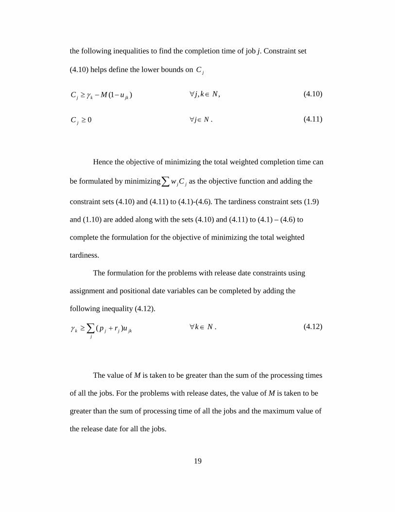
19

the following inequalities to find the completion time of job j. Constraint set

(4.10) helps define the lower bounds on jC

(1 )j k jkC M uγ≥ − − , ,j k N∀ ∈ (4.10)

0≥jC Nj∈∀ . (4.11)

Hence the objective of minimizing the total weighted completion time can

be formulated by minimizing∑ jjCw as the objective function and adding the

constraint sets (4.10) and (4.11) to (4.1)-(4.6). The tardiness constraint sets (1.9)

and (1.10) are added along with the sets (4.10) and (4.11) to (4.1) – (4.6) to

complete the formulation for the objective of minimizing the total weighted

tardiness.

The formulation for the problems with release date constraints using

assignment and positional date variables can be completed by adding the

following inequality (4.12).

∑ +≥j

jkjjk urp )(γ Nk∈∀ . (4.12)

The value of M is taken to be greater than the sum of the processing times

of all the jobs. For the problems with release dates, the value of M is taken to be

greater than the sum of processing time of all the jobs and the maximum value of

the release date for all the jobs.

20

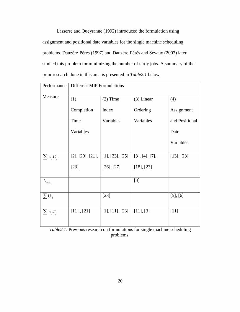
Lasserre and Queyranne (1992) introduced the formulation using

assignment and positional date variables for the single machine scheduling

problems. Dauzère-Pérès (1997) and Dauzère-Pérès and Sevaux (2003) later

studied this problem for minimizing the number of tardy jobs. A summary of the

prior research done in this area is presented in Table2.1 below.

Performance

Measure

Different MIP Formulations

(1)

Completion

Time

Variables

(2) Time

Index

Variables

(3) Linear

Ordering

Variables

(4)

Assignment

and Positional

Date

Variables

∑ jj Cw [2], [20], [21],

[23]

[1], [23], [25],

[26], [27]

[3], [4], [7],

[18], [23]

[13], [23]

maxL [3]

∑ jU [23] [5], [6]

∑ jjTw [11] , [21] [1], [11], [23] [11], [3] [11]

Table2.1: Previous research on formulations for single machine scheduling problems.

21

3. Computational Comparison of the Formulations

3.1. Data Sets

We run our experiments for different set of parameters for all of these four

formulations. We adopt the idea of parameter selection presented by Hariri and

Potts (1983), Potts and Van Wassenhove (1982, 1983), and Abdul-Razaq et al.

(1990).

For each job j, an integer processing time, jp , is generated from uniform

distribution [1, 100] and [1, 10] and an integer weight jw is generated from the

uniform distribution [1, 10]. The due date, jd , of job j is an integer generated

from the uniform distribution [P (L-R/2), P (L+R/2)], where P is the sum of

processing times of all jobs and the two parameters L and R are relative measures

of the location and range of the distribution, respectively. The release date,jr , of

job j is an integer generated from the uniform distribution [0, QP], where P is the

sum of processing times of all the jobs and the parameter Q defines the range of

the distribution. We choose L from the set L ∈ {0.5, 0.7}, R is chosen from the set

R ∈ {0.4, 0.8, 1.4}, and Q is taken as 0.4, which makes the release date

distribution range to be [0, 0.4P]. We run 3 problem instances for each of the six

different combinations of L and R, generating a total of 18 runs for each of the

four different formulations for the problems. Also we restrict our computation to

L ∈ {0.5} for the problems with release dates, thus reducing from 18 to 9 runs for

22

different formulations. The number of jobs, n, is chosen from the set n ∈ {20, 40,

60, 100}.

3.2. Results

The MIP formulations are modeled using AMPL and CPLEX 8.1 with

default settings is used to solve the generated problem instances. The experiments

are run on a Linux distributed machine with a 2.4 GHz processor and 1GB

memory. The runs are terminated after an hour of CPU time.

To compare the different formulations arising from the choice of different

variables, we look at the objective function value of the LP relaxation, the number

of nodes explored, the computational time for the problem instances for which the

optimal solution is obtained within one hour, the number of tests cases unsolved

in one hour, and the optimality gap for the instances that could not be solved

within one hour. The formulations are also compared based on the number of test

instances in which either the optimal or the best feasible solution (in case the

optimal is not found by any formulation) is obtained by each formulation.

The results obtained for total weighted completion time, maximum

lateness, number of tardy jobs and total weighted tardiness objectives when there

are no release dates are presented in Tables2.2, 2.3, 2.4 and 2.5, respectively.

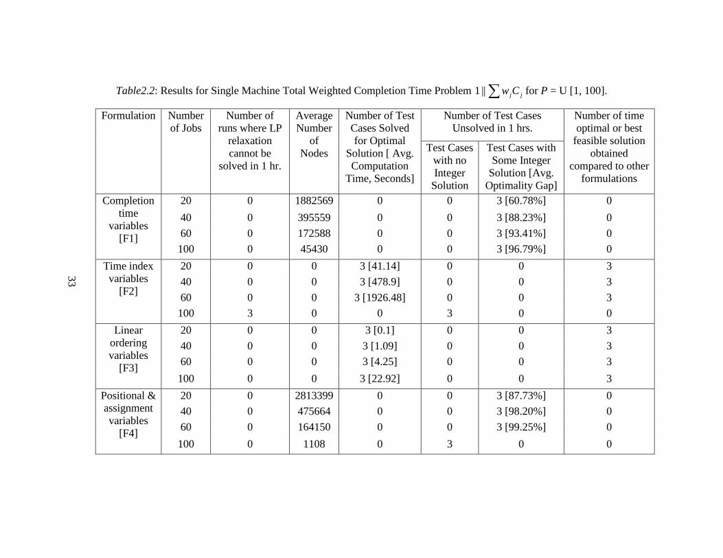
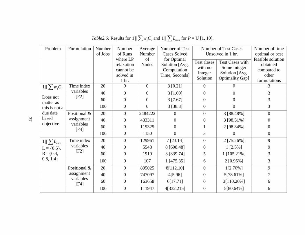
For the ∑ jj Cw objective (see Table2.2) without release dates we test only

3 instances because the parameters L and R are irrelevant as this objective is not

due date based. For this objective, F3 (formulation with linear ordering variables)

23

performed the best. It turns out that the LP relaxation of this formulation reduces

to the Weighted Shortest Processing Time (WSPT) rule, which gives the optimal

solution for this problem. Hence even the test cases with 100 jobs were solved

within 23 seconds. Similarly, F2 (formulation with time index variables) was also

able to provide the optimal solution at the root node, but the computation time

increased exponentially as the number jobs increased and the test cases with 100

jobs were not solved within one hour of computational time. F1 (formulation with

completion time variables) and F4 (formulation with assignment and positional

date variables) did not perform well for this problem. These formulations were

able to solve the LP relaxation much faster but the bounds obtained were not tight

enough to converge to the optimal solution within one hour of computational

time.

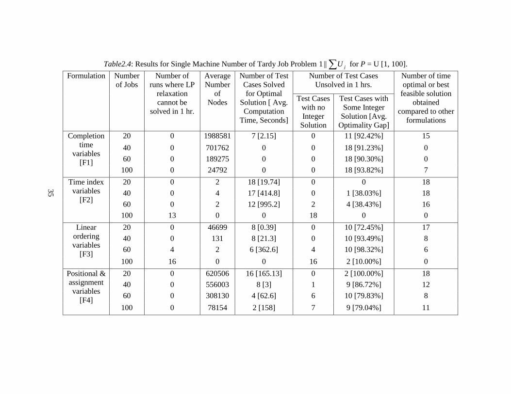
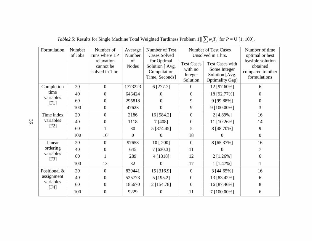
The results obtained for the other three objectives

(∑ maxL ,∑ jU and∑ jjTw ) without the release dates were similar. The findings

from the computations reported in Tables2.3, 2.4 and 2.5 are summarized below:

• All formulations have difficulty as the number of jobs increases (increase in

the computational time).

• F1 and F2 do not produce optimal solution as frequently as F3 and F4 when

the number of jobs is increased. It is obvious that F2 does not perform well

because as the number of jobs increases, we are not even able to solve the LP

relaxation. F1 solves the LP relaxation faster, but that does not help us very

much as the bound is not tight.

24

• F4 often finds a feasible solution, but the optimality gap is higher than F3

because the lower bound obtained by the LP relaxation of F4 is not as tight as

the one for F3. Further, the number of test instances unsolved with F3 is much

higher than with F4 when the number of jobs increases. This is because it gets

harder to solve the LP relaxation of F3 as the number of jobs increases.

• Overall it is harder to solve the LP relaxations of F2 and F3 with an increased

number of jobs, though the bounds are tighter. With F1 and F4, it is easier to

solve the LP relaxations, but the bounds are not very tight. Comparatively, the

number of test cases solved that have either the optimal solution or the best

feasible solution is much higher for F4 but usually with a large optimality gap.

• F4 might be the choice of formulation for an expert in integer programming

because the LP relaxation of this formulation can be solved faster and a larger

number of nodes can be explored in a fixed amount of time. This creates a

potential to use the recent advancements in integer programming literature

(e.g. branch and cut).

Based on our personal communication with Queyranne (2004), we decided

to make additional experiments, since the performance of F2 is known to be

highly influenced by the sum of the processing times. An initial set of

computational experiments was done on the total weighted tardiness problem. The

results of these experiments are presented in Khowala et al. (2005). In these

experiments the processing times are created from the discrete uniform

25

distribution [1, 10]. As expected, F2 was found to be much more efficient with a

lower range of processing times. This is because the number of the variables of F2

is a function of the sum of the processing times of the jobs and the LP relaxation

is much easier to solve when the sum of the processing times of the jobs is small.

But as the number of jobs increases, F2 was not able to give even a feasible

solution. It was also observed that F1 and F4 also perform better with the lower

range of processing times because the value of big M in F1 and F4 depends on the

sum of the processing times of the jobs. However improvements for F4 were more

than those for F1. The performance of F3 was not affected by changing the range

of the processing times because the constraints of F3 do not contain processing

times.

We tested F2 and F4 to see the effect of reducing the processing time

range. We only tested the instances with L=0.5 to reduce the number of

experiments. These results are presented in Tables2.6 and 2.7. F2 is more efficient

with lower ranges of processing times, but as we increase the number of jobs

(therefore the sum of the processing times), the performance of F2 is reduced.

Further we conducted a similar series of experiments for these four

problems with release dates. We limit out experimentations to 9 runs for each

formulation and each different number of jobs by selecting L = 0.5. As mentioned

earlier, the value of Q is selected as 0.4 to determine the range for the release

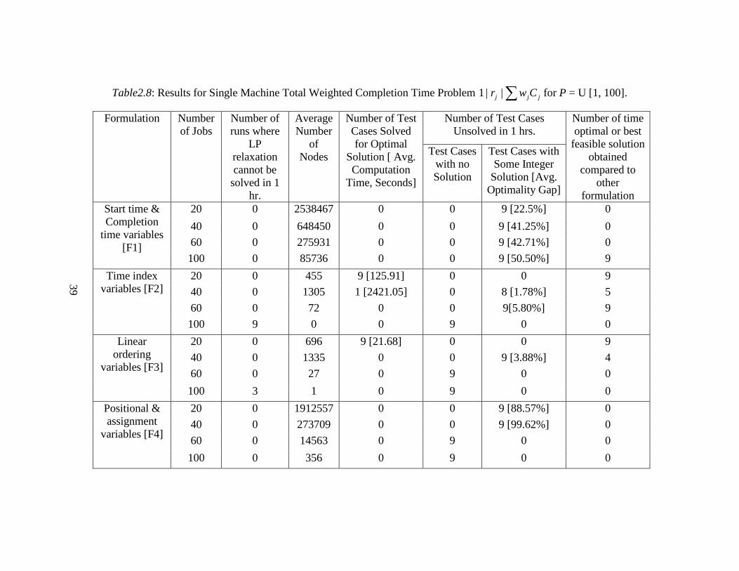
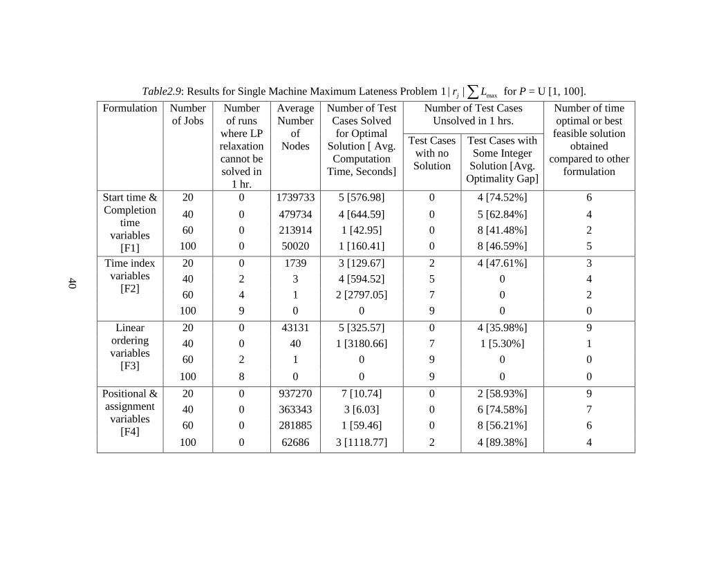
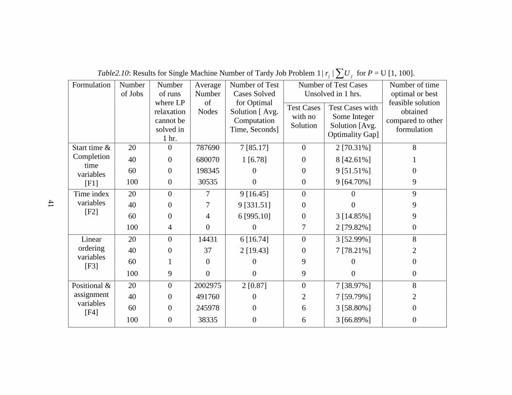
dates. These results are presented in Tables2.8, 2.9, 2.10 and 2.11. The findings

from the computational results can be summarized below for the problems with

release dates:

26

• F3 can no longer solve the LP relaxation for the ∑ jj Cw problem when there

are release dates.

• F1, F3 and F4 do not produce an optimal solution as frequently as the F2

formulation for most of the problems (except for the∑ maxL , which we feel

could also behave the same if we allowed the computation to run longer than 1

hour). F2 is either able to provide an optimal solution with an increasing

larger number of jobs (up to 60 jobs) or is within an optimality gap of 30%.

• F1 and F4 often find a feasible solution, but the optimality gap is higher than

F2, because the lower bound obtained by the LP relaxation of F1 and F4 are

not as tight as the one obtained from F2.

• F3 also provides much tighter lower bounds compared to F1 and F4, but the

LP relaxation is much harder to solve. For most of the test instances F3

terminated without any solution.

• The comparison of the quality of solution (comparing the optimal or the best

feasible solution) obtained from the four formulations also indicate that F2

performs the best and also the performance of F2 is better with increasing

number of jobs (except as noted above for∑ maxL ). The increase in the

efficiency of F2 after adding the release date constraints can be attributed to

the reduction in the time index variables for these problems. The release data

constraints forces the time index variables to be zero for the values of t < jr .

27

• F2 should be the choice with the release date constraints for the test cases we

investigated.

4. Improved Assignment and Positional date Formulation

The computational results presented in the subsequent sections and also in

Khowala et. al. (2005), suggested that the bounds obtained from the formulations

using time index variables and linear ordering variables were tighter than those

from the other formulations but the LP relaxations were harder to solve, hence the

branch and bound algorithm would not be able to explore a large number of nodes

given a fixed computational time budget. On the other hand, the LP relaxation of

the formulation with assignment and positional variables was easy to solve but the

bounds were not tight enough to yield a better feasible solution within a given

computation time. Hence we further studied this formulation and came up with

two families of valid inequalities that help in improving the lower bounds

obtained from this formulation. The first family of valid inequalities will also help

us to remove the big-M constraints given by (4.10) and the second set of

inequalities gives a better lower bound on completion time variables. The

inequalities assume that the jobs are arranged in non decreasing order of the

processing times, i.e. nppp ≤≤≤≤ ......0 21 .

28

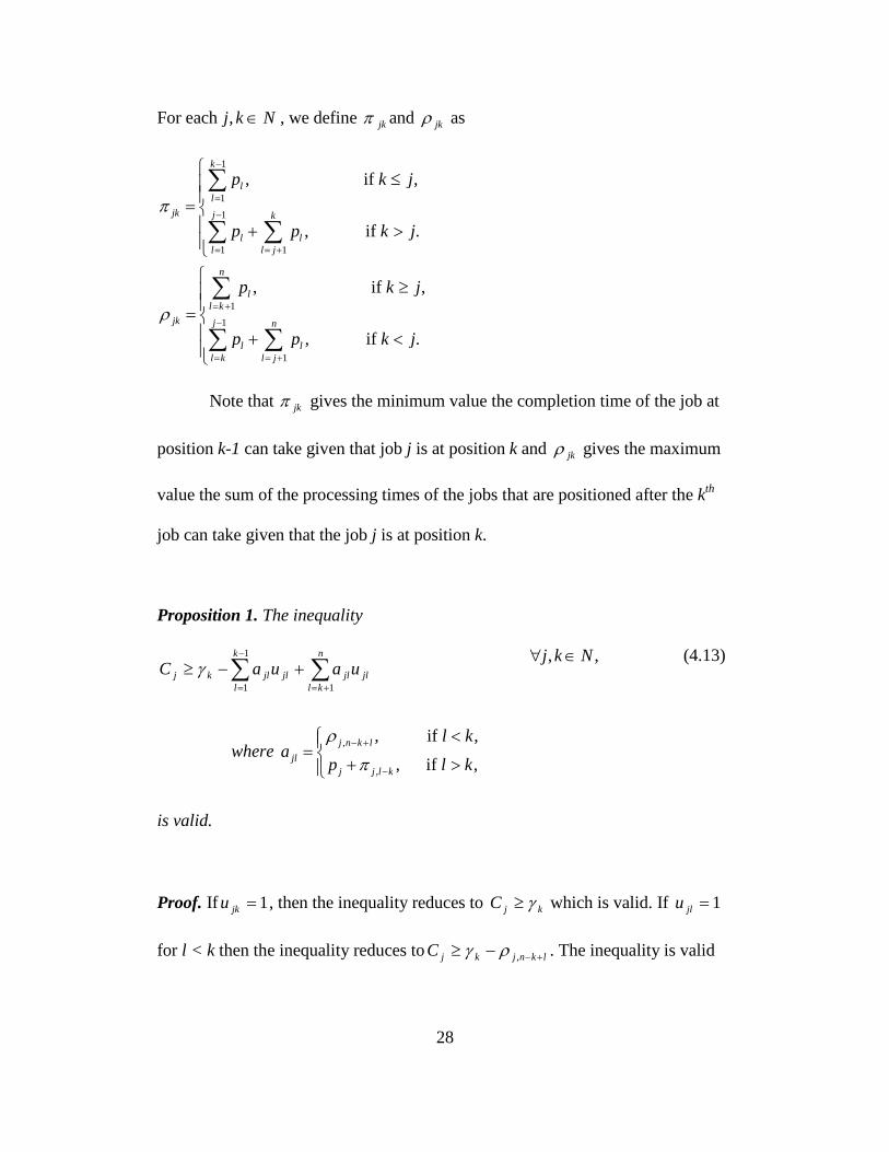
For each Nkj ∈, , we define jkπ and jkρ as

1

1

1

1 1

1

1

1

, if ,

, if .

, if ,

, if .

k

ll

jk j k

l ll l j

n

ll k

jk j n

l ll k l j

p k j

p p k j

p k j

p p k j

π

ρ

−

=

−

= = +

= +

−

= = +

≤

= + >

≥

= + <

∑

∑ ∑

∑

∑ ∑

Note that jkπ gives the minimum value the completion time of the job at

position k-1 can take given that job j is at position k and jkρ gives the maximum

value the sum of the processing times of the jobs that are positioned after the kth

job can take given that the job j is at position k.

Proposition 1. The inequality

∑∑+=

−

=

+−≥n

kljljl

k

ljljlkj uauaC

1

1

1

γ , ,j k N∀ ∈ (4.13)

where ,

,

, if ,

, if ,j n k l

jlj j l k

l ka

p l k

ρ

π− +

−

<=

+ >

is valid.

Proof. If 1=jku , then the inequality reduces to kjC γ≥ which is valid. If 1=jlu

for l < k then the inequality reduces to lknjkjC +−−≥ ,ργ . The inequality is valid

29

for this case because lknjkl +−−≥ ,ργγ from the definition of s'ρ . If 1=jlu for l

> k then the inequality reduces to jkljkj pC ++≥ −,πγ . The inequality is valid for

this case because jkljkl p++≥ −,πγγ from the definition of s'π .

Also note that when 1=jku the inequality (4.13) forces kjC γ≥ , therefore

the inequalities given by (4.10) can be replaced by (4.13).

Proposition 2. For a job Nj ∈ , the inequality

∑=

+≥n

kjkjkjj upC

2

π (4.14)

is valid.

Proof. If the job j is at position k>1 then 1=jku and (4.14) becomes

jkjj pC π+≥ and is valid from the definition of sjk 'π .

4.1. Computational Performance of the Improved Formulation

Our findings so far, suggest F4 worked consistently well across most of

the problems without release dates. F4 could be improved significantly for some

problems by adding the new set of inequalities described in the previous section.

We conducted an additional set of computational experiments by replacing the

equation (4.10) by these two new set of inequalities (4.13) and (4.14) for

the ∑ jjCw||1 and ∑ jjTw||1 problems. The results are presented in Table2.12 for

30

the cases where the processing times are from the discrete uniform distribution [1,

10], L = {0.5} and R = {0.4, 0.8, 1.4} and in Table2.13 for the cases where the

processing times are from the discrete uniform distribution [1, 100], L = {0.5,

0.7} and R = {0.4, 0.8, 1.4}.

The results obtained for these two objectives had a similar pattern, both

for the original formulation as well as for the improved formulation. The findings

from the computational experiments reported in Tables2.12 and 2.13 are

summarized below:

• The original formulation using the assignment and positional variables for

both of these problem solves the LP relaxation faster, but that does not help us

very much as the bound is not tight and the test instances end up with the

optimality gaps between 50% and 100% in one hour of computational time.

For most of the test cases the lower bounds generated by LP relaxations are

equal to zero. Also, the original formulation often finds a feasible solution but

the optimality gap is higher.

• After adding these two new classes of inequalities, the bounds obtained were

much tighter (almost for all of the test instances the objective value of LP

relaxation with improved formulation was better), which helped in obtaining

the optimal solutions for larger number of test instances as well as reducing

the optimality gap to 5% - 20% range for ∑ jj Cw problem and to 35% - 85%

range for ∑ jjTw problem.

31

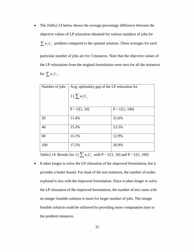
• The Table2.14 below shows the average percentage difference between the

objective values of LP relaxation obtained for various numbers of jobs for

∑ jj Cw problem compared to the optimal solution. These averages for each

particular number of jobs are for 3 instances. Note that the objective values of

the LP relaxations from the original formulation were zero for all the instances

for ∑ jj Cw .

Number of jobs Avg. optimality gap of the LP relaxation for

∑ jjCw||1

P ~ U[1, 10] P ~ U[1, 100]

20 11.4% 31.6%

40 15.3% 23.3%

60 15.1% 12.9%

100 17.5% 20.9%

Table2.14: Results for ∑ jjCw||1 with P ~ U[1, 10] and P ~ U[1, 100]

• It takes longer to solve the LP relaxation of the improved formulation, but it

provides a better bound. For most of the test instances, the number of nodes

explored is less with the improved formulation. Since it takes longer to solve

the LP relaxation of the improved formulation, the number of test cases with

no integer feasible solution is more for larger number of jobs. The integer

feasible solution could be achieved by providing more computation time to

the problem instances.

32

For some instances where a feasible solution can not be found easily,

primal heuristics could help us to find one easily. The fractional optimal solution

found at a node can be modified to satisfy the integrality conditions. Suppose that

at a node the solution ( *** ,, Cu γ ) has at least one (j, k) pair such that jku that is

fractional. We can sort the job indices in non-decreasing order of the completion

time variables *C . These job indices will give us a feasible schedule and an upper

bound to the problem. Our preliminary experiments showed that this primal

heuristic gives solutions that are either optimal or very close to the optimal after a

few number of nodes are explored. These results are not given here as the main

focus of this paper is to compare the formulations with default settings of a

commercial solver.

33

Table2.2: Results for Single Machine Total Weighted Completion Time Problem ∑ jjCw||1 for P = U [1, 100].

33

Formulation Number of Jobs

Number of runs where LP

relaxation cannot be

solved in 1 hr.

Average Number

of Nodes

Number of Test Cases Solved for Optimal

Solution [ Avg. Computation

Time, Seconds]

Number of Test Cases Unsolved in 1 hrs.

Number of time optimal or best

feasible solution obtained

compared to other formulations

Test Cases with no Integer

Solution

Test Cases with Some Integer

Solution [Avg. Optimality Gap]

Completion time

variables [F1]

20 0 1882569 0 0 3 [60.78%] 0

40 0 395559 0 0 3 [88.23%] 0

60 0 172588 0 0 3 [93.41%] 0

100 0 45430 0 0 3 [96.79%] 0

Time index variables

[F2]

20 0 0 3 [41.14] 0 0 3

40 0 0 3 [478.9] 0 0 3

60 0 0 3 [1926.48] 0 0 3

100 3 0 0 3 0 0

Linear ordering variables

[F3]

20 0 0 3 [0.1] 0 0 3

40 0 0 3 [1.09] 0 0 3

60 0 0 3 [4.25] 0 0 3

100 0 0 3 [22.92] 0 0 3

Positional & assignment variables

[F4]

20 0 2813399 0 0 3 [87.73%] 0

40 0 475664 0 0 3 [98.20%] 0

60 0 164150 0 0 3 [99.25%] 0

100 0 1108 0 3 0 0

34

Table2.3: Results for Single Machine Maximum Lateness Problem ∑ max||1 L for P = U [1, 100].

34




solved in 1 hr.

Average Number

of Nodes



Time, Seconds]






Solution



Completion time

variables [F1]

20 0 1938442 5 [2.93] 0 13 [344.84%] 16

40 0 559034 4 [5.29] 0 14 [276.4%] 14

60 0 213123 3 [62.77] 0 15 [341.40%] 10

100 0 41459 0 1 17 [243.97%] 9


[F2]

20 0 269 6 [767.6] 3 9 [147.54%] 6

40 12 4 3 [413.6] 15 0 3

60 18 0 0 18 0 0

100 18 0 0 18 0 0


[F3]

20 0 192698 6 [0.18] 0 12 [156.16%] 18

40 0 232 6 [557.4] 12 0 6

60 0 2 3 [239.1] 15 0 3

100 16 0 0 18 0 0


[F4]

20 0 259094 17 [6.7] 0 1 [34.41%] 18

40 0 623075 10 [40.52] 0 8 [149.73%] 12

60 0 382129 6 [30.66] 0 12 [87.40%] 8

100 0 86241 7 [261.93] 0 11 [102.20%] 12

35

Table2.4: Results for Single Machine Number of Tardy Job Problem ∑ jU||1 for P = U [1, 100].

35




solved in 1 hr.

Average Number

of Nodes



Time, Seconds]






Solution



Completion time

variables [F1]

20 0 1988581 7 [2.15] 0 11 [92.42%] 15

40 0 701762 0 0 18 [91.23%] 0

60 0 189275 0 0 18 [90.30%] 0

100 0 24792 0 0 18 [93.82%] 7


[F2]

20 0 2 18 [19.74] 0 0 18

40 0 4 17 [414.8] 0 1 [38.03%] 18

60 0 2 12 [995.2] 2 4 [38.43%] 16

100 13 0 0 18 0 0


[F3]

20 0 46699 8 [0.39] 0 10 [72.45%] 17

40 0 131 8 [21.3] 0 10 [93.49%] 8

60 4 2 6 [362.6] 4 10 [98.32%] 6

100 16 0 0 16 2 [10.00%] 0


[F4]

20 0 620506 16 [165.13] 0 2 [100.00%] 18

40 0 556003 8 [3] 1 9 [86.72%] 12

60 0 308130 4 [62.6] 6 10 [79.83%] 8

100 0 78154 2 [158] 7 9 [79.04%] 11

36

Table2.5: Results for Single Machine Total Weighted Tardiness Problem ∑ jjTw||1 for P = U [1, 100].

36




solved in 1 hr.

Average Number

of Nodes



Time, Seconds]






Solution



Completion time

variables [F1]

20 0 1773223 6 [277.7] 0 12 [97.60%] 6

40 0 646424 0 0 18 [92.77%] 0

60 0 295818 0 9 9 [99.88%] 0

100 0 47623 0 9 9 [100.00%] 3


[F2]

20 0 2186 16 [584.2] 0 2 [4.89%] 16

40 0 1118 7 [408] 0 11 [10.26%] 14

60 1 30 5 [874.45] 5 8 [48.70%] 9

100 16 0 0 18 0 0


[F3]

20 0 97658 10 [ 200] 0 8 [65.37%] 16

40 0 645 7 [630.3] 11 0 7

60 1 289 4 [1318] 12 2 [1.26%] 6

100 13 32 0 17 1 [1.47%] 1


[F4]

20 0 839441 15 [316.9] 0 3 [44.65%] 16

40 0 525773 5 [195.2] 0 13 [83.42%] 6

60 0 185670 2 [154.78] 0 16 [87.46%] 8

100 0 9229 0 11 7 [100.00%] 6

37

Table2.6: Results for ∑ jjCw||1 and ∑ max||1 L for P = U [1, 10].

37

Problem Formulation Number of Jobs

Number of Runs

where LP relaxation cannot be solved in

1 hr.

Average Number

of Nodes


Solution [Avg. Computation

Time, Seconds]

Number of Test Cases Unsolved in 1 hr.



compared to other

formulations


Solution



∑ jjCw||1

Does not matter as this is not a due date based objective


[F2]

20 0 0 3 [0.21] 0 0 3

40 0 0 3 [1.69] 0 0 3

60 0 0 3 [7.67] 0 0 3

100 0 0 3 [38.3] 0 0 3


[F4]

20 0 2484222 0 0 3 [88.48%] 0

40 0 433311 0 0 3 [98.51%] 0

60 0 119325 0 1 2 [98.84%] 0

100 0 1150 0 3 0 0

∑ max||1 L

L = {0.5}, R= {0.4, 0.8, 1.4}


[F2]

20 0 129961 7 [23.14] 0 2 [75.26%] 9

40 0 5548 8 [698.48] 0 1 [2.5%] 9

60 0 1919 3 [839.74] 5 1 [105.21%] 3

100 0 107 1 [475.35] 6 2 [0.95%] 3


[F4]

20 0 895025 8[112.10] 0 1[2.70%] 9

40 0 747097 4[5.96] 0 5[78.61%] 7

60 0 163658 6[17.71] 0 3[110.20%] 6

100 0 111947 4[332.215] 0 5[80.64%] 6

38

Table2.7: Results for ∑ jU||1 and ∑ jjTw||1 for P = U [1, 10].

38


Number of Runs


1 hr.

Average Number

of Nodes


Solution [Avg. Computation

Time, Seconds]






Solution



∑ jU||1

L = {0.5}, R= {0.4, 0.8, 1.4}


[F2]

20 0 0 9 [0.18] 0 0 9

40 0 3 9 [2.05] 0 0 9

60 0 10 9 [15.84] 0 0 9

100 0 31 9 [119.1] 0 0 9

Positional &

assignment variables

[F4]

20 0 693528 7[1.00] 0 2[38.29%] 9

40 0 727446 2[22.43] 0 7[46.94%] 4

60 0 145725 5[44.18] 0 4[17.05%] 5

100 0 82411 1[92.81] 3 5[24.18%] 1

∑ jjTw||1

L = {0.5}, R= {0.4, 0.8, 1.4}


[F2]

20 0 65 9 [1.02] 0 0 9

40 0 31848 9 [255.4] 0 0 9

60 0 6568 9 [194.2] 0 0 9

100 0 37130 2 [633.74] 0 7 [2.67%] 9

Positional &

assignment variables

[F4]

20 0 1777692 4 [86.48] 0 5 [46.92%] 4

40 0 799491 0 0 9 [85.70%] 0

60 0 238139 0 0 9 [91.43%] 0

100 0 8569 0 2 7 [98.65%] 0

39

Table2.8: Results for Single Machine Total Weighted Completion Time Problem ∑ jjj Cwr ||1 for P = U [1, 100].

39


Number of runs where

LP relaxation cannot be solved in 1

hr.

Average Number

of Nodes



Time, Seconds]




compared to other

formulation

Test Cases with no Solution



Start time & Completion

time variables [F1]

20 0 2538467 0 0 9 [22.5%] 0

40 0 648450 0 0 9 [41.25%] 0

60 0 275931 0 0 9 [42.71%] 0

100 0 85736 0 0 9 [50.50%] 9

Time index variables [F2]

20 0 455 9 [125.91] 0 0 9

40 0 1305 1 [2421.05] 0 8 [1.78%] 5

60 0 72 0 0 9[5.80%] 9

100 9 0 0 9 0 0

Linear ordering

variables [F3]

20 0 696 9 [21.68] 0 0 9

40 0 1335 0 0 9 [3.88%] 4

60 0 27 0 9 0 0

100 3 1 0 9 0 0

Positional & assignment

variables [F4]

20 0 1912557 0 0 9 [88.57%] 0

40 0 273709 0 0 9 [99.62%] 0

60 0 14563 0 9 0 0

100 0 356 0 9 0 0

40

Table2.9: Results for Single Machine Maximum Lateness Problem ∑ max||1 Lr j for P = U [1, 100].

40


Number of runs


1 hr.

Average Number

of Nodes



Time, Seconds]




compared to other formulation





time variables

[F1]

20 0 1739733 5 [576.98] 0 4 [74.52%] 6

40 0 479734 4 [644.59] 0 5 [62.84%] 4

60 0 213914 1 [42.95] 0 8 [41.48%] 2

100 0 50020 1 [160.41] 0 8 [46.59%] 5


[F2]

20 0 1739 3 [129.67] 2 4 [47.61%] 3

40 2 3 4 [594.52] 5 0 4

60 4 1 2 [2797.05] 7 0 2

100 9 0 0 9 0 0


[F3]

20 0 43131 5 [325.57] 0 4 [35.98%] 9

40 0 40 1 [3180.66] 7 1 [5.30%] 1

60 2 1 0 9 0 0

100 8 0 0 9 0 0


[F4]

20 0 937270 7 [10.74] 0 2 [58.93%] 9

40 0 363343 3 [6.03] 0 6 [74.58%] 7

60 0 281885 1 [59.46] 0 8 [56.21%] 6

100 0 62686 3 [1118.77] 2 4 [89.38%] 4

41

Table2.10: Results for Single Machine Number of Tardy Job Problem ∑ jj Ur ||1 for P = U [1, 100].

41


Number of runs


1 hr.

Average Number

of Nodes



Time, Seconds]









time variables

[F1]

20 0 787690 7 [85.17] 0 2 [70.31%] 8

40 0 680070 1 [6.78] 0 8 [42.61%] 1

60 0 198345 0 0 9 [51.51%] 0

100 0 30535 0 0 9 [64.70%] 9


[F2]

20 0 7 9 [16.45] 0 0 9

40 0 7 9 [331.51] 0 0 9

60 0 4 6 [995.10] 0 3 [14.85%] 9

100 4 0 0 7 2 [79.82%] 0


[F3]

20 0 14431 6 [16.74] 0 3 [52.99%] 8

40 0 37 2 [19.43] 0 7 [78.21%] 2

60 1 0 0 9 0 0

100 9 0 0 9 0 0


[F4]

20 0 2002975 2 [0.87] 0 7 [38.97%] 8

40 0 491760 0 2 7 [59.79%] 2

60 0 245978 0 6 3 [58.80%] 0

100 0 38335 0 6 3 [66.89%] 0

42

Table2.11: Results for Single Machine Total Weighted Tardiness Problem ∑ jjj Twr ||1 for P = U [1, 100].

42


Number of runs


1 hr.

Average Number

of Nodes



Time, Seconds]









time variables

[F1]

20 0 2464169 2 [1694.83] 0 7 [61.86%] 2

40 0 836104 0 0 9 [68.39%] 0

60 0 297155 0 0 9 [71.82%] 0

100 0 72422 0 0 9 [77.62%] 9


[F2]

20 0 5285 7 [74.35] 0 2 [4.68%] 8

40 0 1890 3 [1434.45] 0 6 [8.47%] 9

60 0 296 0 0 9 [28.51%] 9

100 9 0 0 9 0 0


[F3]

20 0 41777 6 [444.13] 0 3 [12.38%] 9

40 0 110 0 9 0 0

60 5 2 0 9 0 0

100 9 0 0 9 0 0


[F4]

20 0 2366900 1 [21.93] 0 8 [59.95%] 1

40 0 406505 0 0 9 [96.17%] 0

60 0 122699 0 1 8 [96.92%] 0

100 0 936 0 9 0 0

43

Table2.12: Results for ∑ jjCw||1 and ∑ jjTw||1 for P = U [1, 10] with improved inequalities

43


Average Number

of Nodes

Number of Test Cases Solved for Optimal Solution

[Avg. Computation

Time, Seconds]






Solution



∑ jjCw||1



[F4]

20 2484222 0 0 3 [88.48%] 0

40 433310 0 0 3 [98.51%] 3

60 119324 0 1 2 [98.83%] 2

100 1150 0 3 0 0


(improved formulation)

20 539638 0 0 3 [6.15%] 3

40 40257 0 2 1 [27.25%] 0

60 6373 0 3 0 0

100 9 0 3 0 0

∑ jjTw||1

L = {0.5}, R= {0.4, 0.8, 1.4}


[F4]

20 1777692 4 [86.48] 0 5 [46.92%] 4

40 799491 0 0 9 [85.70%] 5

60 238139 0 0 9 [91.43%] 4

100 8569 0 2 7 [98.65%] 7



20 436811 6 [439.7] 0 3 [35.65%] 8

40 98731 0 0 9 [60.58%] 5

60 25570 0 1 8 [69.29%] 5

100 651 0 9 0 0

44

Table2.13: Results for ∑ jjCw||1 and ∑ jjTw||1 for P = U [1, 100] with improved inequalities

44


Average Number

of Nodes

Number of Test Cases Solved for Optimal Solution

[Avg. Computation

Time, Seconds]






Solution



∑ jjCw||1



[F4]

20 2813399 0 0 3 [87.73%] 1

40 475664 0 0 3 [98.20%] 1

60 164150 0 0 3 [99.25%] 0

100 1108 0 3 0 0



20 528710 0 0 3 [9.11%] 2

40 49645 0 0 3 [22.18%] 2

60 7734 0 0 3 [22.87%] 3

100 43 0 3 0 0

∑ jjTw||1

L = {0.5, 0.7}, R= {0.4, 0.8, 1.4}


[F4]

20 839441 15 [316.9] 0 3 [44.65%] 16

40 525773 5 [195.2] 0 13 [83.42%] 7

60 185670 2 [154.78] 0 16 [87.46%] 8

100 9229 0 11 7 [100.00%] 7



20 778305 18 [216.25] 0 0 18

40 105692 6 [473.3] 0 12 [64.34%] 14

60 26871 2 [353.68] 3 13 [80.13%] 11

100 732 0 15 3 [100.00%] 1

45

5. Conclusion and Future Work

In this paper we have compared the computational performance of four

different formulations on single machine scheduling problems with varying

complexity. The performances of these formulations very much depend on the

objective function, number of jobs and the sum of the processing times of all the

jobs. F2 and F3 appear to be the most widely used formulations in the Integer

Programming and Scheduling literature and F4 appears to be the least widely

used. F1 often appears in textbooks and other literature that simply

formulate/describe the problem (not the solution methodology) and it clearly does

not generally perform well in practice.

With F1 and F4, the LP relaxation is easy to solve and provides a feasible

solution easily. F2 and F3 have been preferred due to the fact that they generally

produce tighter bounds. However, we have found that the LP relaxation of these

formulations tends to be much more difficult to solve. This is particularly true for

F2 when P (sum of processing time of all the jobs) is large. Therefore fewer nodes

of the branch and bound tree can be explored for a fixed computational budget.

This limits one’s ability to explore recent advancement in IP methodology (such

as branch and cut). On the other hand, the LP relaxation of F4 can be solved

relatively quickly, so this MIP formulation offers more promise for these new

advanced techniques. In Section 4 we gave two simple families of inequalities

that improved the bounds obtained from the LP- relaxation. A more detailed

46

polyhedral study would make this formulation work better. We note that when P

is small or with release date constraints, F2 becomes the preferred formulation.

There was noticeable improvement in terms of achieving a better bound

(LP relaxation) and reduction in the optimality gap by adding the new set of

inequalities to F4 and removing the big-M constraint. Further if we are able to

trade off the solution quality (in terms of reducing the optimality gap and

obtaining better integer feasible solution) versus the computational time, this new

formulation will be preferred, as we can notice the improvement in the solution

quality.

We are aware that for most of the problems studied in this paper problem

specific algorithms have been proposed and they are shown to be more effective

than solving MIP formulations. But it should be noted that these are problem

specific algorithms and require expertise in coding and scheduling. Also these

algorithms are hard to modify for other problems in the same domain. The MIP

formulations studied in this paper on the other hand could be easily solved using

commercial solvers and don’t require expertise in scheduling or coding.

This paper is, as of our knowledge, the first paper that compares the

computational performances of these four MIP formulations in the scheduling

literature. As future research, the MIP formulations can be compared with other

additional restrictions, such as precedence constraints, or for more complex

machine environments. F4 might be the choice of formulation for an expert in

integer programming because the LP relaxation of this formulation can be solved

47

faster and a larger number of nodes can be explored in a fixed amount of

computational time. This creates a potential to use recent advancements found in

the integer programming literature. Studying the polyhedral structure of this

formulation and using the valid inequalities at a branch-and-cut algorithm is the

subject of a forthcoming paper.

48

References

1. Abdul-Razaq, T. S., Potts, C. N., & Van Wassenhove, L. N. (1990). A survey of algorithms for the single machine total weighted tardiness scheduling problem. Discrete Applied Mathematics, 26, 235-253. 2. Balas, E. (1985). On the facial structure of scheduling polyhedra. Mathematical Programming, 24, 179-218. 3. Blazewicz, J., Dror, M., & Weglarz, J. (1991). Mathematical programming formulations for machine scheduling: A survey. European Journal of Operational Research, 51, 283-300. 4. Chudak, F. A., & Hochbaum, D. S. (1999). A half-integral linear programming relaxation for scheduling precedence-constrained jobs on a single machine. Operations Research Letters, 25, 199-204. 5. Dauzère-Pérès, S. (1997). An efficient formulation for minimizing the number of late jobs in single-machine scheduling. IEEE Symposium on Emerging Technologies & Factory Automation (ETFA), 442-445. 6. Dauzère-Pérès, S., & Sevaux, M. (2003). Using Lagrangean relaxation to minimize the weighted number of late jobs on a single machine. Naval Research Logistics, 50(3), 273-288. 7. Dyer, M. E., & Wolsey, L. A. (1990). Formulating the single machine sequencing problem with release dates as a mixed integer program. Discrete Applied Mathematics, 26, 255-270. 8. Graham, R. L., Lawler, E. L., Lenstra, J. K., & Rinnooy Kan, A. H. G. (1979). Optimization and approximation in deterministic sequencing and scheduling: a survey. Annals of Discrete Mathematics, 5, 287-326. 9. Hariri, A. M. A., & Potts, C. N. (1983). An algorithm for single machine sequencing with release dates to minimize total weighted completion time. Discrete Applied Mathematics, 5, 99-109. 10. Jackson, J. R. (1955). Scheduling a production line to minimize maximum tardiness. Management Science Research Project, (Research Report 43) University of California, Los Angles. 11. Khowala, K., Keha, A. B., & Fowler, J. (2005). A comparison of different formulations for the non-preemptive single machine total weighted tardiness

49

scheduling problem. The Second Multidisciplinary International Conference on Scheduling: Theory & Application (MISTA). 12. Kise, H., Ibaraki, T., & Mine, H. (1978). A solvable case of the one-machine scheduling problem with ready and due times. Operations Research, 26, 121-126. 13. Lasserre, J. B., & Queyranne, M. (1992). Generic scheduling polyhedral and a new mixed-integer formulation for single-machine scheduling. Proceedings of the Second IPCO Conference, Carnegie-Mellon University, Pittsburgh, 136-149. 14. Lawler, E. L. (1977). A ‘pseudopolynomial’ time algorithm for sequencing jobs to minimize total tardiness. Annals of Discrete Mathematics, 1, 331-342. 15. Lenstra, J. K., Rinnooy Kan, A. H. G., & Brucker, P. (1977). Complexity of machine scheduling problems. Annals of Discrete mathematics, 1, 343-362. 16. Moore, J. M. (1968). An n job, one machine sequencing algorithm for minimizing the number of late jobs. Management Science, 15, 102-109. 17. Nemhauser, G. L., & Savelsbergh, M. W. P. (1992). A cutting plane algorithm for the single machine scheduling problem with release times. Combinatorial Optimization: New Frontiers in the Theory and Practice (M. Akgül, H. Hamacher and S. Tufecki, eds.), NATO ASI Series F: Computer and Systems Sciences, Springer: Berlin, 82, 63-84. 18. Potts, C. N., & Van Wassenhove, L. N. (1983). An algorithm for single machine sequencing with deadlines to minimize total weighted completion time. European Journal of Operational Research, 12, 379-389. 19. Potts, C. N., & Van Wassenhove, L. N. (1982). A decomposition algorithm for the single machine, total tardiness problem. Operations Research Letters, 1, 177-181. 20. Queyranne, M., & Wang, Y. (1991). Single-machine scheduling polyhedra with precedence constraints. Mathematics of Operations Research, 16, 1-20. 21. Queyranne, M. (1993). Structure of a simple scheduling polyhedron. Mathematical Programming, 58, 263-285. 22. Queyranne, M. (2004). Personal Communication at INFORMS Annual Conference, Denver, October, 2004.

50

23. Queyranne, M., & Schulz, A. S. (1994). Polyhedral approaches to machine scheduling. Technical Report 408/1994, Department of Mathematics, Technical University of Berlin, Berlin, Germany. 24. Smith, W. E. (1956). Various optimizers for single stage production. Naval Research Logistics Quarterly, 3, 59-66. 25. Šorić, K. (2000). A cutting plane algorithm for a single machine scheduling problem. European Journal of Operational Research, 127, 383-393. 26. Sousa, J. P., & Wolsey, L. A. (1992). A time-indexed formulation of non-preemptive single-machine scheduling problems. Mathematical programming, 54, 353-367. 27. Van den Akker, J.M., van Hoesel, C. P. M., & Savelsbergh, M.W.P. (1999). A Polyhedral approach to single machine scheduling problems. Mathematical Programming, 85, 541-572.

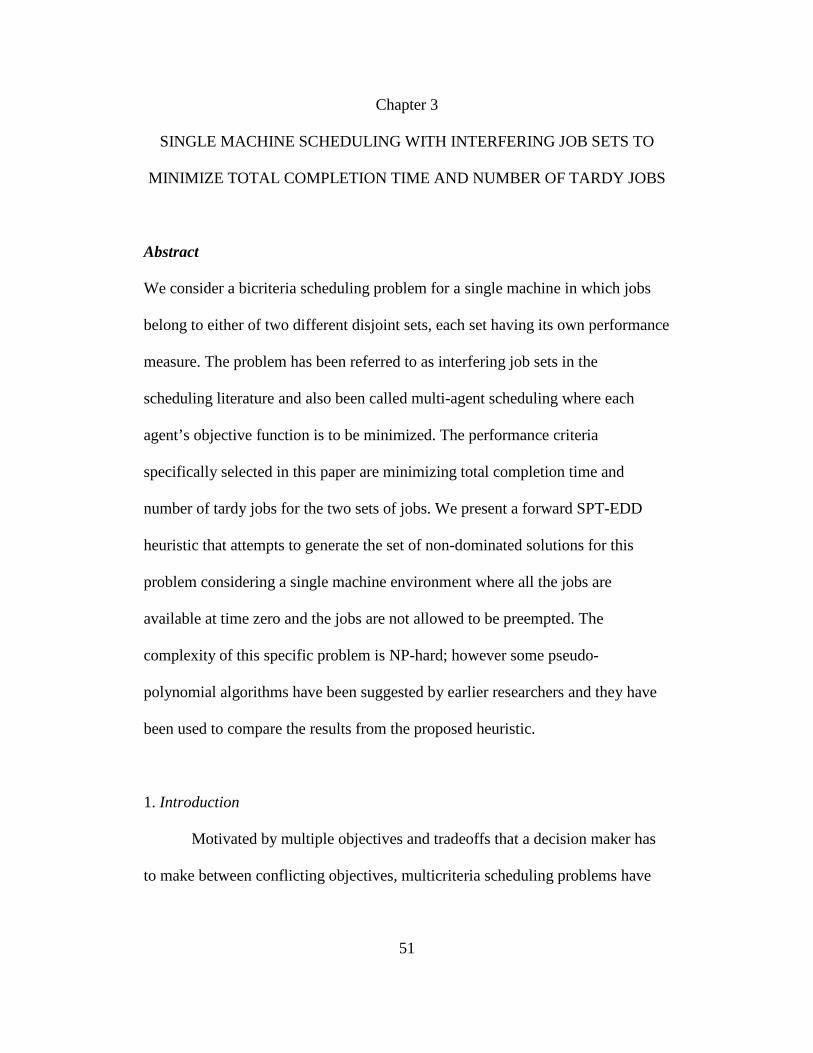
51

Chapter 3

SINGLE MACHINE SCHEDULING WITH INTERFERING JOB SETS TO

MINIMIZE TOTAL COMPLETION TIME AND NUMBER OF TARDY JOBS

Abstract

We consider a bicriteria scheduling problem for a single machine in which jobs

belong to either of two different disjoint sets, each set having its own performance

measure. The problem has been referred to as interfering job sets in the

scheduling literature and also been called multi-agent scheduling where each

agent’s objective function is to be minimized. The performance criteria

specifically selected in this paper are minimizing total completion time and

number of tardy jobs for the two sets of jobs. We present a forward SPT-EDD

heuristic that attempts to generate the set of non-dominated solutions for this

problem considering a single machine environment where all the jobs are

available at time zero and the jobs are not allowed to be preempted. The

complexity of this specific problem is NP-hard; however some pseudo-

polynomial algorithms have been suggested by earlier researchers and they have

been used to compare the results from the proposed heuristic.

1. Introduction

Motivated by multiple objectives and tradeoffs that a decision maker has

to make between conflicting objectives, multicriteria scheduling problems have

52

been widely dealt with in the literature (see T’Kindt et al. [2006]). In this domain

of scheduling problems one typically has to satisfy multiple criteria on the same

set of jobs. However, in some cases jobs belong to different job sets and must be

processed using the same resource, hence causing interference. These job sets can

have different criteria to be optimized. These different sets may represent

customers or agents whose requirements may differ. The complexity of this

domain of problems depends on the number of job sets considered, the specific

performance criteria considered, restrictions on each set of jobs; and the machine

environment.

One of the earliest references on this subject is Peha [1995] which dealt

with the problem of interfering job sets with objectives of minimizing weighted

number of tardy jobs in one set and total weighted completion time in another set

of jobs with unit processing time under an identical parallel machine environment.

The assumption of unit processing times makes the problem easier to solve. The

paper from Baker and Smith [2003] was the first paper formalizing scheduling

problems with interfering job sets. They considered a single machine problem

involving the minimization of criteria including makespan, maximum lateness,

and total weighted completion time ),,( maxmax ∑ jj CwLC . They showed that any

combination of these criteria on different job sets can be solved in polynomial

time by defining the optimization function as a linear combination of the criteria

on different job sets, except for the combination of ∑ jj Cw and maxL on different

job sets which turns out to be NP-hard.

53

Agnetis et al. [2004] presented the complexity of generating non-

dominated solutions for single machine as well as shop floor scheduling problems

with interfering job sets, involving objectives of minimizing total completion

time, total number of tardy jobs and total weighted completion

time ),,( ∑∑∑ jjjj CwUC . Ng et al. [2006] proved that the problem involving

jobs sets with total completion time and total number of tardy jobs on a single

machine is NP-hard under high multiplicity encoding and have presented a

pseudo polynomial time algorithm for this problem. Further, Leung et al. [2010]

proved that the interfering jobs sets problem with total completion time and total

number of tardy jobs on a single machine is NP-hard. Cheng et al. [2006] have

shown NP completeness of the problem where jobs belong to one of the multiple

sets and each set has the objective of minimizing the total weighted number of

tardy jobs )(∑ jjUw . They also presented a polynomial time approximation

scheme for this problem. In one of the most recent works, Balasubramanian et al.

[2008] presented a heuristic that attempts to generate all the non-dominated points

for the interfering job sets on a parallel machine environment with the criteria of

minimizing maximum lateness on one set of jobs and total completion time on

another set of jobs. The paper proposes an iterative SPT-LPT-SPT heuristic and a

bicriteria genetic algorithm for the problem by exploiting the structure of the

problem and provide a comparison of the computational efficiency with a time

index MIP formulation.

54

Wan et al. [2009, 2010] dealt with two agent scheduling problems with

controllable processing times, where the cost of compression is included in the

objective function of the first agent. The machine environment is single or

identical parallel machines and the criteria included are total completion time,

maximum tardiness, maximum lateness, etc. Lee et al. [2011] developed a

branch-and-bound algorithm and a simulated annealing heuristic algorithm to

address a two machine flow shop problem with two agents. The objectives

considered were to minimize the total completion time for the first agent with no

tardy jobs for the second agent.

Khowala et al. [2009] dealt with two interfering job sets on a single

machine with the objectives of minimizing total completion time and total number

of tardy jobs for the two sets, respectively. A forward SPT-EDD heuristic was

proposed that attempts to generate the Pareto-Optimal frontier. Further the

objective of minimizing total weighted completion time and maximum lateness

was dealt with in Khowala et al. [2011].

In the subsequent sections, we define the problem, talk about the structure

of the problem and some key properties of the problem, present heuristics to

generate the efficient frontier, and compare the computational performance of the

near non-dominated solution sets obtained from our heuristic with the Pareto

optimal solution sets obtained by the pseudo polynomial algorithm of Ng et al.

[2006].

55

2. Problem Description

The specific problem that we are looking into relates to single machine

scheduling where all jobs are available at time zero and no preemption is allowed.

We look at the single machine problem with interfering jobs from two disjoint

sets, one having the objective of minimizing total completion time and the other

minimizing the total number of tardy jobs. As discussed earlier, the complexity of

this problem is NP-hard (Leung et al. [2010]). A pseudo- polynomial algorithm is

presented by Ng et al. [2006] for this problem under binary encoding. We

combine some of the intuition from Moore’s algorithm (Moore [1968]) to

determine the initial set of jobs that can be on time and then use a forward SPT-

EDD heuristic to determine all the non dominated points for this problem.

There are two disjoint interfering sets of jobs 1ξ and 2ξ with n1 and n2

number of jobs in each respective set. The total number of jobs that need to be

scheduled is n = (n1 + n2). We seek to minimize the total completion time of the

jobs in first set 1ξ and for the jobs in second set 2ξ we want to minimize the total

number of tardy jobs. The processing times of the jobs in set 1ξ and sets2ξ are

represented by 1jp and 2jp , respectively. Similarly the due dates for the jobs in the

first set and the second set are denoted by 1jd and 2

jd , respectively. However, for

the purpose of the objectives considered herein, due dates are only relevant for the

jobs in the second set.

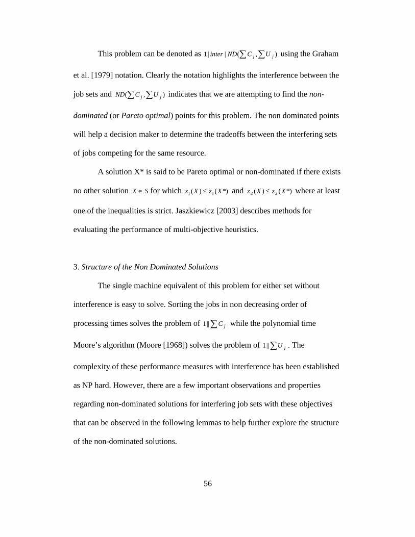
56

This problem can be denoted as ),(||1 ∑∑ jj UCNDinter using the Graham

et al. [1979] notation. Clearly the notation highlights the interference between the

job sets and ),( ∑∑ jj UCND indicates that we are attempting to find the non-

dominated (or Pareto optimal) points for this problem. The non dominated points

will help a decision maker to determine the tradeoffs between the interfering sets

of jobs competing for the same resource.

A solution X* is said to be Pareto optimal or non-dominated if there exists

no other solution SX ∈ for which *)()( 11 XzXz ≤ and *)()( 22 XzXz ≤ where at least

one of the inequalities is strict. Jaszkiewicz [2003] describes methods for

evaluating the performance of multi-objective heuristics.

3. Structure of the Non Dominated Solutions

The single machine equivalent of this problem for either set without

interference is easy to solve. Sorting the jobs in non decreasing order of

processing times solves the problem of ∑ jC||1 while the polynomial time

Moore’s algorithm (Moore [1968]) solves the problem of ∑ jU||1 . The

complexity of these performance measures with interference has been established

as NP hard. However, there are a few important observations and properties

regarding non-dominated solutions for interfering job sets with these objectives

that can be observed in the following lemmas to help further explore the structure

of the non-dominated solutions.

57

Lemma 4.1.1: There always exists a non-delay schedule for all the strongly non-

dominated points on the Pareto optimal front.

Lemma 4.1.2(a): For all the strongly non-dominated points, there exists an

optimal schedule in which jobs in the job set1ξ are scheduled in SPT order (see Ng

et al. [2006]).

Lemma 4.1.2(b): For all the strongly non-dominated points, there exists an

optimal schedule in which jobs in the job set2ξ that are on time are scheduled in

EDD order (see Ng et al. [2006]).

Lemma 4.1.3: For any non-dominated point for this problem, the performance

criteria∑ jC , for the jobs in the job set1ξ with preemptive scheduling remains the

same as with non preemptive scheduling, provided the jobs in job set 2ξ which

caused the preemption are scheduled before the job that got preempted from1ξ .

We define three subset of jobs1S , 2S and 3S . Based on the above

observation, for any non-dominated point, the subset of jobs1S will contain all the

jobs from 1ξ arranged in SPT order, another subset2S of on time jobs from

set 2ξ which will be in EDD order and a third subset3S of jobs that are tardy from

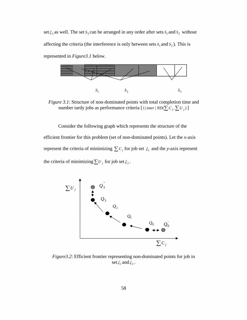
58

set 2ξ as well. The set3S can be arranged in any order after sets1S and 2S without

affecting the criteria (the interference is only between sets1S and 2S ). This is

represented in Figure3.1 below.

1S 2S 3S

Figure 3.1: Structure of non-dominated points with total completion time and number tardy jobs as performance criteria [ ),(||1 ∑∑ jj UCNDinter ]

Consider the following graph which represents the structure of the

efficient frontier for this problem (set of non-dominated points). Let the x-axis

represent the criteria of minimizing ∑ jC for job set 1ξ and the y-axis represent

the criteria of minimizing∑ jU for job set 2ξ .

Figure3.2: Efficient frontier representing non-dominated points for job in set 1ξ and 2ξ .

∑ jU

∑ jC

0Q

2Q

1Q '0Q

'3Q

3Q

59

The points 0Q , 1Q , 2Q and 3Q in the above graph in Figure3.2 represent the

strongly non-dominated points on the efficient frontier. The point 3Q gives the

best value of total completion time for jobs in set1ξ . Similarly 0Q gives the best

value of total number of jobs that are on time from set2ξ . The point '0Q is a point

which is weakly non-dominated by the jobs in set1ξ and point '3Q is weakly non-

dominated by the jobs in set2ξ . The strongly non-dominated point 0Q can be

represented by ∑∑ = min,||1 YUCinter jj , where minY is the minimum number of

tardy jobs obtained by solving ∑ jU||1 for the second set without interference.

Similarly the non-dominated point 3Q can be represented by

∑∑ = jj UKCinter ,||1 min , where minK is the minimum number of total completion

time obtained by solving ∑ jC||1 for first set without interference. Note that only

the point ∑∑ = jj UKCinter ,||1 min is polynomial time solvable. We can get this

point by scheduling all the jobs in set1ξ first by SPT order followed by all the jobs

in set 2ξ using Moore’s Algorithm (to apply Moore’s algorithm at this particular

point we will have to increase the processing times of all the jobs in set 2ξ by the

value of minK ).

4. Forward SPT-EDD Heuristic

Based on the earlier discussion on the structure of non-dominated points,

the efficient frontier of the first problem and the few distinct properties

60

(Lemma4.1.1, Lemma4.1.2a, Lemma4.1.2b and Lemma4.1.3) of the problem

discussed so far, we present a forward SPT-EDD algorithm that attempts to

generate the non-dominated points for this problem. In the forward logic

presented below, we start with Moore’s algorithm to determine the initial

sets 2S and 3S . In the subsequent section we compare the computational efficiency

of this algorithm with the optimal solutions from the pseudo polynomial

algorithm of Ng et al. [2006].

The Forward SPT-EDD algorithm for this problem can be summarized

in the following steps, where we start from the initial point

∑∑ = min,||1 YUCinter jj (i.e. 0Q ) and then determine the next point by moving

jobs from set 2S to 3S until we reach the point ∑∑ = jj UKCinter ,||1 min (i.e. 3Q ):

Step 1: Use Moore’s algorithm to determine the minimum number of tardy jobs

by considering jobs in set2ξ alone. The solution from Moore’s algorithm will help

determine the sets2S and 3S . The tardy jobs are placed in set3S while the on time

jobs will be placed in set2S . Note: This step may result in a non-dominated

solution that is not Pareto optimal, as the division between jobs from 2ξ in sets

2S and 3S obtained by Moore’s algorithm, may not result in the best possible value

for ∑ jC for jobs in the first set.

61

Step2: With this initial division for set2ξ into sets 2S and 3S , a non-dominated

solution is determined for interfering jobs sets1S and 2S using Lemma4.1.2(a) and

Lemma4.1.2(b).

Step 3: First the jobs in set2S are arranged in EDD order in such a way that there

is no earliness for the jobs in set2S , except when there is an overlap between jobs

within set 2S . In case of overlap, jobs with earlier due dates are placed ahead of

jobs with later due dates. Now the jobs in set1S are arranged in SPT order

allowing preemption. We finally use the property described in Lemma4.1.3 to get

the non preemptive schedule for this non-dominated point.

Now, consider Restriction 1 under which the jobs that were tardy at one

non-dominated point will also remain tardy at the next non-dominated point as we

move in the direction of improving∑ jC (i.e. jobs from set3S are not allowed to

move back to set2S ).

Lemma 5.1.1: Under the above restriction, the one job that needs to be moved

from set 2S to set 3S (new jobs become tardy as we move to the next non-

dominated point) will be the one which when moved from set2S to set 3S provides

the best preemptive schedule for all the jobs in job set1S without moving the

position of other jobs in set2S (hence the best improvement in the value of total

completion time).

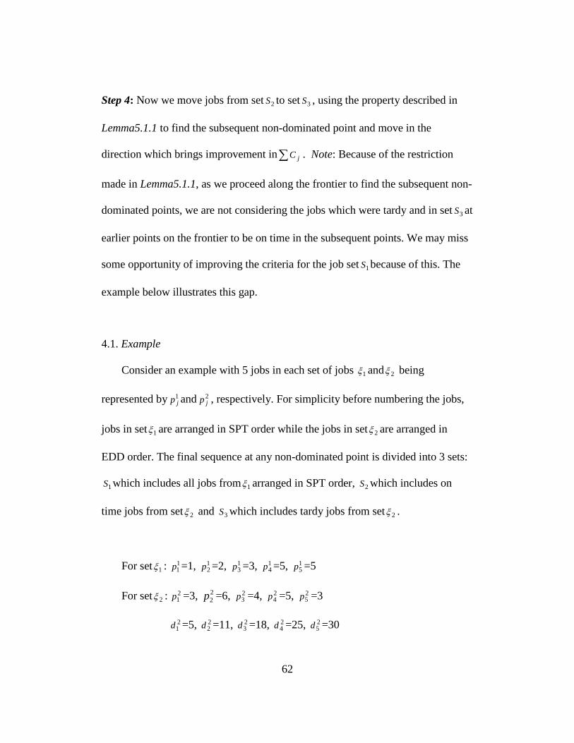
62

Step 4: Now we move jobs from set2S to set 3S , using the property described in

Lemma5.1.1 to find the subsequent non-dominated point and move in the

direction which brings improvement in∑ jC . Note: Because of the restriction

made in Lemma5.1.1, as we proceed along the frontier to find the subsequent non-

dominated points, we are not considering the jobs which were tardy and in set3S at

earlier points on the frontier to be on time in the subsequent points. We may miss

some opportunity of improving the criteria for the job set1S because of this. The

example below illustrates this gap.

4.1. Example

Consider an example with 5 jobs in each set of jobs 1ξ and 2ξ being

represented by1jp and 2

jp , respectively. For simplicity before numbering the jobs,

jobs in set1ξ are arranged in SPT order while the jobs in set2ξ are arranged in

EDD order. The final sequence at any non-dominated point is divided into 3 sets:

1S which includes all jobs from1ξ arranged in SPT order, 2S which includes on

time jobs from set2ξ and 3S which includes tardy jobs from set2ξ .

For set 1ξ : 11p =1, 1

2p =2, 13p =3, 1

4p =5, 15p =5

For set 2ξ : 21p =3, 2

2p =6, 23p =4, 2

4p =5, 25p =3

21d =5, 2

2d =11, 23d =18, 2

4d =25, 25d =30

63

The value of ∑ jC for problem ∑ jC||1 is 37, while∑ jU for

problem ∑ jU||1 is zero. In iteration (1) since all the jobs in set2ξ are on time, 2S =

{1, 2, 3, 4, 5} and 3S = { }. Jobs in set 1S are arranged in SPT order while jobs in

set 2S are arranged in EDD order. This results in point 0Q (101, 0).

Time Horizon1 2 3 4 5 6 7 8 9 10 11 12 13 14 15 16 17 18 19 20 21 22 23 24 25 26 27 28 29 30 31 32 33 34 35 36 37

1 2 3 4 51 1 2 2 3 3 4 5 4 5

Figure3.3(a): In the first step jobs in 1S are allowed to be preempted. In the second step jobs in set 2S are moved ahead to avoid preemption of jobs in set1S .

Note that the completion time of the jobs in 1S remains the same.

In iteration (2), it is found that moving job #2 from set2S to 3S will provide

maximum improvement in∑ jC , hence 2S = {1, 3, 4, 5} and 3S = {2}. This gives

the non-dominated point 1Q (61, 1).

Time Horizon1 2 3 4 5 6 7 8 9 10 11 12 13 14 15 16 17 18 19 20 21 22 23 24 25 26 27 28 29 30 31 32 33 34 35 36 37

1 3 4 5 21 1 2 3 4 3 4 5 5 2

Figure3.3(b): In the first step job #2 from set 2S is moved to 3S and jobs in set

1S are allowed to be preempted. In the second step jobs in set 2S are moved ahead to avoid preemption of jobs in set1S . Note that the completion time of the jobs in

1S remains the same.

64

In iteration (3) it is found that moving job #1 from set2S to 3S will provide

maximum improvement in∑ jC , hence 2S = {3, 4, 5} and 3S = {2, 1}. This gives


Time Horizon1 2 3 4 5 6 7 8 9 10 11 12 13 14 15 16 17 18 19 20 21 22 23 24 25 26 27 28 29 30 31 32 33 34 35 36 37

3 4 5 2 11 2 3 4 3 5 4 5 2 1

Figure3.3(c): In the first step job #1 from set 2S is moved to 3S and jobs in set

1S are allowed to be preempted. In the second step jobs in set 2S are moved ahead to avoid preemption of jobs in set1S . Note that the completion time of the jobs in

1S remains the same.

In iteration (4) it is found that moving job #3 from set2S to 3S will provide

maximum improvement in∑ jC , hence 2S = {4, 5} and 3S = {2, 1, 3}. This gives


Time Horizon1 2 3 4 5 6 7 8 9 10 11 12 13 14 15 16 17 18 19 20 21 22 23 24 25 26 27 28 29 30 31 32 33 34 35 36 371 2 3 4 5 4 5 2 1 3

Figure3.3(d): Job #3 from set 2S is moved to 3S and jobs in set 1S are already in a non preemptive SPT order.

Now since the best possible value of∑ jC is 37, making more jobs tardy

will not provide any further improvement in∑ jC , hence will result in weakly

non-dominated points: 4Q (37, 4) and 5Q (37, 5).

65

5. Dynamic Program Algorithm

Ng et al. (2006) has proposed a pseudo-polynomial algorithm for the

),(||1 ∑∑ jj UCNDinter problem that provides the optimal solutions sets. We

use this algorithm to compare the solution quality of our heuristic. Based on the

Dynamic Program proposed by Ng et al. (2006), the optimal value is given by

),,,(min 210 2 YDnnRPD≤≤

, where Y is the restriction imposed on the number of

tardy jobs and ∑≤≤

=21

)2(2

njjpP , sum of processing time of all the jobs in set 2ξ . The

number of jobs in set 1ξ and 2ξ are represented by 1n and 2n , respectively. The

complexity of this pseudo-polynomial algorithm is given by )( 2221 PnnO which

relates to the maximum number of states in the Dynamic Program. Ng et al.

(2006) can be referenced for further details on this approach.

6. Computational Experiments

We compare the computational efficiency and solution quality of our

heuristic for this problem with the optimal solutions by generating 120 problem

instances for various numbers of jobs in each set. For the symmetric scenarios, we

consider cases with 20, 30, 40 and 50 jobs in each set1ξ and 2ξ and generate

twenty problem instances for each case. Further, for the asymmetric scenario, we

consider cases with 10 and 30 jobs in set1ξ and 2ξ . We select integer processing

time numbers for both sets of jobs from ~ U [1, 20]. The due date,jd , of job j is

an integer generated from the uniform distribution [P (L-R/2), P (L+R/2)], where

66

P = 0.5 P1 + P2 (P1 is the sum of processing time in of jobs in set1ξ and P2 is the

sum of processing time of jobs in set2ξ ) and the two parameters L and R are

relative measures of the location and range of the distribution, respectively. This

particular methodology of generating the due date ranges is adopted from Abdul-

Razaq et al. [1990] and has been used in other papers as well (Keha et al. [2009]).

We choose L ∈ {0.5, 0.7} and R ∈ {0.4, 0.8} to generate four different ranges of

due dates: [0.3 P, 0.7P], [0.1 P, 0.9P], [0.5 P, 0.9P] and [0.3 P, 1.1P]; and

generate five problem instances for each range, hence generating twenty problem

instances in total for each number of jobs. To test the computational efficiency we

have selected up to 100 job problem instances (50 jobs in each set).

The heuristic and the dynamic programming algorithm are coded using

MATLAB 2009b. The experiments were run on a windows machine with 1.66

GHz processor and 2.5GB memory.

7. Results

To test the performance of the Forward SPT-EDD heuristic for our first

problem ),(|int|1 jj UCNDer ∑ , we compare the non-dominated solutions sets with

the results from the pseudo-polynomial algorithm of Ng et al. [2006].

Column 4 of Table3.1 presents the average computational time for the

heuristic over 20 different problem instances (5 instances for 4 different due date

ranges) for each number of jobs. It can be observed that the computational time

for the pseudo polynomial DP algorithm (column 5 of Table3.1) grows faster with

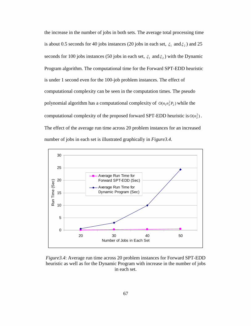
67

the increase in the number of jobs in both sets. The average total processing time

is about 0.5 seconds for 40 jobs instances (20 jobs in each set, 1ξ and 2ξ ) and 25

seconds for 100 jobs instances (50 jobs in each set, 1ξ and 2ξ ) with the Dynamic

Program algorithm. The computational time for the Forward SPT-EDD heuristic

is under 1 second even for the 100-job problem instances. The effect of

computational complexity can be seen in the computation times. The pseudo

polynomial algorithm has a computational complexity of )( 2221 PnnO while the

computational complexity of the proposed forward SPT-EDD heuristic is )( 22nO .

The effect of the average run time across 20 problem instances for an increased

number of jobs in each set is illustrated graphically in Figure3.4.

0

5

10

15

20

25

30

20 30 40 50Number of Jobs in Each Set

Run

Tim

e (S

ec)

Average Run Time forForward SPT-EDD (Sec)

Average Run Time forDynamic Program (Sec)

Figure3.4: Average run time across 20 problem instances for Forward SPT-EDD heuristic as well as for the Dynamic Program with increase in the number of jobs

in each set.

68

In Table3.1 we also summarize the comparison of average solution quality

over 120 problem instances (80 instances with a symmetric number of jobs in

each set and 40 instances with an asymmetric number of jobs in each set) obtained

from the heuristic with the optimal solution obtained from the pseudo-polynomial

DP algorithm. As expected, the average number of strongly non-dominated points

generated by the DP (column 6) increases with the increase in the number of jobs

in each set. Column 7 reflects the average number of non Pareto optimal points

from the heuristic. Note that even with the increase in the average number of non

Pareto optimal points (column 7), the average percentage gap between the

strongly non dominated points generated from the Dynamic Program and by the

Forward SPT-EDD heuristic (column 8) is 0.50% or under for all symmetric

problem instances. Note that this gap in fact decreases as the number of jobs

increases from 20 in each set to 50 in each set (even though the average number

of non Pareto optimal points within a solution set increases). Thus, this table

illustrates that the heuristic performs very well in comparison to the DP. While

the DP is also fast (25 seconds computation time in 50 job instances), the heuristic

uses simple intuitive rules and hence will be easier to implement in practice even

for a very large number of jobs sets. We note that the DP memory explodes for

problem instances with more then 50 jobs in each set.

For the asymmetric problem instances, the average percentage gap

between strongly non dominated points generated from the Dynamic Program and

the Forward SPT-EDD heuristic is much lower (about 0.02%) for the 30-10 job

69

instances compared to about 2% for the 10-30 job instances (10 jobs in job set 1ξ

and 30 jobs in job set 2ξ ). The reason for the relatively higher errors on 1:3

asymmetries compared to 3:1 is well explained by the structure of the problem

and the design of the Forward SPT-EDD heuristic which restricts the tardy jobs to

become non-tardy as we move along the efficient frontier (jobs from set 3S do not

move back to set2S ). With a higher number of jobs in 2ξ compared to1ξ there

will often be an opportunity to improve the solution quality with some pair wise

swaps. For all practical purposes we consider 1:3 asymmetries as the extreme case

and even for these instances the errors are below 2%. This suggests that a

corrective pair-wise swap algorithm will produce a negligible increase in solution

quality and hence may not be necessary.

8. Conclusion and Future Research

The proposed polynomial heuristic does a good job of providing a near

non dominated solution set; the average gap is less than 1% compared to the

optimal solution. The computational experiment could be extended to see the

effect of the increased run time with a larger number of jobs with the pseudo-

polynomial algorithm. However, we note that the DP memory explodes for

problem instances with more then 50 jobs in each set. It can be clearly seen that

this SPT-EDD heuristic performs quite well and will be useful in solving job sets

each with a larger number of jobs e.g. 200 or higher. A similar approach could be

adopted to solve other interfering job set problems with different performance

70

criteria; even problems which have been classified as NP-hard. We further intend

to carry our more computational experiments as well as explore the structure of

the single machine problems with two interfering job sets with criterion of total

weighted completion time and number of tardy jobs as well as total weighted

completion time and maximum lateness. Further it will be interesting to see if the

EDD rule will still hold for on time jobs or jobs with the criteria of minimizing

maximum lateness when interfering with another job set that has the criterion to

minimize total weighted completion time.

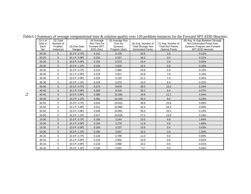
71

Table3.1:Summary of average computational time & solution quality over 120 problem instances for the Forward SPT-EDD Heuristic.

71

(1) # of Jobs in Each Set

(2) Total Number of Problem Instances

(3) Due Date Ranges

(4) Average Run Time for Forward SPT-

EDD (Sec)

(5) Average Run Time for Dynamic

Program (Sec)

(6) Avg. Number of Total Strongly Non Dominated Points

(7) Avg. Number of Total Non Pareto Optimal Points

(8) Avg. % Gap Between Strongly Non Dominated Points from

Dynamic Program and Forward SPT-EDD Heuristic

20-20 5 [0.3 P, 0.7P] 0.151 0.478 20.8 3.6 0.12%

20-20 5 [0.1 P, 0.9P] 0.152 0.527 16.2 3.2 0.21%

20-20 5 [0.5 P, 0.9P] 0.154 0.573 14.4 3.8 0.50%

20-20 5 [0.3 P, 1.1P] 0.150 0.626 15.4 6.8 0.33%

30-30 5 [0.3 P, 0.7P] 0.219 2.880 29.8 5.0 0.10%

30-30 5 [0.1 P, 0.9P] 0.218 2.811 24.8 7.6 0.19%

30-30 5 [0.5 P, 0.9P] 0.225 3.120 21.2 7.4 0.34%

30-30 5 [0.3 P, 1.1P] 0.223 3.073 15.0 6.4 0.31%

40-40 5 [0.3 P, 0.7P] 0.373 9.878 39.2 13.0 0.16%

40-40 5 [0.1 P, 0.9P] 0.359 9.418 35.2 9.4 0.07%

40-40 5 [0.5 P, 0.9P] 0.380 10.283 24.6 11.2 0.34%

40-40 5 [0.3 P, 1.1P] 0.361 10.419 20.4 9.0 0.23%

50-50 5 [0.3 P, 0.7P] 0.535 23.915 49.8 15.8 0.08%

50-50 5 [0.1 P, 0.9P] 0.511 23.884 42.4 18.4 0.09%

50-50 5 [0.5 P, 0.9P] 0.546 24.891 35.0 16.0 0.13%

50-50 5 [0.3 P, 1.1P] 0.517 24.618 27.2 13.6 0.16%

10-30 5 [0.3 P, 0.7P] 0.156 3.144 13.0 4.8 1.84%

10-30 5 [0.1 P, 0.9P] 0.164 3.279 11.8 4.6 1.89%

10-30 5 [0.5 P, 0.9P] 0.169 3.237 10.6 0.4 0.63%

10-30 5 [0.3 P, 1.1P] 0.180 3.047 10.4 3.6 1.20%

30-10 5 [0.3 P, 0.7P] 0.133 2.788 11.0 0.0 0.00%

30-10 5 [0.1 P, 0.9P] 0.134 2.802 10.8 0.6 0.02%

30-10 5 [0.5 P, 0.9P] 0.133 2.868 10.2 0.6 0.01%

30-10 5 [0.3 P, 1.1P] 0.136 2.931 7.2 0.0 0.00%

72

References

1. Abdul-Razaq, T. S., Potts, C. N., & Van Wassenhove, L. N. (1990). A survey of algorithms for the single machine total weighted tardiness scheduling problem. Discrete Applied Mathematics, 26, 235-253 2. Agnetis, A., Mirchandani, P. B., Pacciarelli, D. & Pacifici, A. (2004). Scheduling problems with two completing agents. Operations Research, 52(2), 229-242. 3. Baker, K. R. & Smith, J. C. (2003). A multiple criterion model for machine scheduling. Journal of Scheduling, 6, 7-16. 4. Balasubramanian H., Fowler J., Keha A. & Pfund M. (2009). Scheduling interfering job sets on parallel machines. European Journal of Operational Research, 199(1), 55-67. 5. Cheng, T.C.E., Ng, C.T. & Yuan, J.J. (2006). Multi-agent scheduling on a single machine to minimize total weighted number of tardy jobs. Theoretical Computer Science, 362, 273-281. 6. Graham, R. L., Lawler, E. L., Lenstra, J. K., & Rinnooy Kan, A. H. G. (1979). Optimization and approximation in deterministic sequencing and scheduling: a survey. Annals of Discrete Mathematics, 5, 287-326. 7. Jaszkiewicz, A. (2003). Evaluation of Multiple Objective Metaheuristics. Lecture Notes in Economics and Mathematical Systems, 535, 65-89. 8. Keha, A., Khowala, K. & Fowler, J. (2009). Mixed integer programming formulations for the single machine scheduling problems. Computers & Industrial Engineering, 56, 357-367. 9. Khowala, K., Fowler, J., Keha, A. & Balasubramanian, H. (2009). Single machine scheduling with interfering job sets. Proceedings of the Multidisciplinary International Scheduling: Theory and Applications Conference (MISTA 2009), 357-365. 10. Khowala, K., Fowler, J., Keha, A. & Balasubramanian, H. (2011). Single machine scheduling with interfering job sets to minimize total weighted completion time and maximum lateness. Proceedings of the Multidisciplinary International Scheduling: Theory and Applications Conference (MISTA 2011), 568-572.

73

11. Lee, W.-C., Chen, S.-K., Chen, C.-W. & Wu, C.-C. (2011). A two-machine flowshop problem with two agents. Computers & Operations Research, 38, 98-104. 12. Leung, J. Y.-T., Pinedo, M. & Wan, G. (2010). Competitive two-agent scheduling and its application. Operations Research, 58(2), 458-469. 13. Moore, J. M. (1968). An n job, one machine sequencing algorithm for minimizing the number of late jobs. Management Science, 15, 102-109. 14. Ng, C.T., Cheng, T.C.E. & Yuan, J.J. (2006). A note on the complexity of the problem of two agent scheduling on a single machine. Journal of Combinatorial Optimization, 12, 387-394. 15. Peha, J. (1995). Heterogeneous-criteria scheduling: minimizing weighted number of tardy jobs and weighted completion time. Journal of Computers and Operations Research, 22(10), 1089-1100. 16. T’Kindt, V., Billaut, J. C. & Scott, H. (2006). Multicriteria Scheduling: Theory, Models and Algorithms. Springer, 2nd edition. 17. Wan, G., Leung, J. Y.-T. & Pinedo, M. (2009). Competitive agent scheduling with Controllable Processing Times. Proceedings of the Multidisciplinary International Scheduling: Theory and Applications Conference (MISTA 2009), 514-522. 18. Wan, G., Vakati, S. R., Leung, J. Y.-T. & Pinedo M. (2010). Scheduling two agent with controllable processing times. European Journal of Operational Research, 205(3), 528-539.

74

Chapter 4

SINGLE MACHINE SCHEDULING WITH INTERFERING JOB SETS TO

MINIMIZE TOTAL WEIGHTED COMPLETION TIME AND MAXIMUM

LATENESS

Abstract

Single machine scheduling with interfering job sets to minimize total weighted

completion time and maximum lateness, is an established NP Hard problem. This

category of problem has also been referred to as multi-agent scheduling (in this

case two agents) where each agent’s objective function is to be minimized. For

the performance criteria specifically selected in this paper, we present a forward

WSPT-EDD heuristic that attempts to generate the set of supported points. We

assume that all the jobs are available at time zero and the jobs are not allowed to

be preempted. We compare the solution quality of the purposed heuristic with

MIP formulations. The framework could also be extended for a similar two job

sets problem on a single machine with total weighted completion time and the

number of tardy jobs as the objective criteria.

1. Introduction

Motivated by multiple objectives and tradeoffs that a decision maker has

to make between conflicting objectives, multicriteria scheduling problems have

been widely dealt with in the literature (see T’Kindt et al. [2006]). In this domain

75

of scheduling problems one typically has to satisfy multiple criteria on the same

set of jobs. However, in some cases jobs belong to different job sets and must be

processed using the same resource, hence causing interference. These job sets can

have different criteria to be optimized. These different sets may represent

customers or agents whose requirements may differ. The complexity of this

domain of problems depends on the number of job sets considered, the specific

performance criteria considered, restrictions on each set of jobs, and the machine

environment.

One of the earliest references on this subject is Peha [1995] which dealt

with the problem of interfering job sets with objectives of minimizing weighted

number of tardy jobs in one set and total weighted completion time in another set

of jobs with unit processing time under an identical parallel machine environment.

The assumption of unit processing times makes the problem easier to solve. The

paper from Baker and Smith [2003] was the first paper formalizing scheduling

problems with interfering job sets. They considered a single machine problem

involving the minimization of criteria including makespan, maximum lateness,

and total weighted completion time ),,( maxmax ∑ jj CwLC . They showed that any

combination of these criteria on different job sets can be solved in polynomial

time by defining the optimization function as a linear combination of the criteria

on different job sets, except for the combination of ∑ jj Cw and maxL on different

job sets which turns out to be NP-hard.

76

Agnetis et al. [2004] presented the complexity of generating non-

dominated solutions for single machine as well as shop floor scheduling problems

with interfering job sets, involving objectives of minimizing total completion

time, total number of tardy jobs and total weighted completion

time ),,( ∑∑∑ jjjj CwUC . Ng et al. [2006] proved that the problem involving

jobs sets with total completion time and total number of tardy jobs on a single

machine is NP-hard under high multiplicity encoding and have presented a

pseudo polynomial time algorithm for this problem. Further, Leung et al. [2010]

proved that the interfering jobs sets problem with total completion time and total

number of tardy jobs on a single machine is NP-hard. Cheng et al. [2006] have

shown NP completeness of the problem where jobs belong to one of the multiple

sets and each set has the objective of minimizing the total weighted number of

tardy jobs )(∑ jjUw . They also presented a polynomial time approximation

scheme for this problem. In one of the most recent works, Balasubramanian et al.

[2008] presented a heuristic that attempts to generate all the non-dominated points

for the interfering job sets on a parallel machine environment with the criteria of

minimizing maximum lateness on one set of jobs and total completion time on

another set of jobs. The paper proposes an iterative SPT-LPT-SPT heuristic and a

bicriteria genetic algorithm for the problem by exploiting the structure of the

problem and provide a comparison of the computational efficiency with a time

index MIP formulation.

77

Wan et al. [2009, 2010] dealt with two agent scheduling problems with

controllable processing times, where the cost of compression is included in the

objective function of the first agent. The machine environment is single or

identical parallel machines and the criteria included are total completion time,

maximum tardiness, maximum lateness, etc. Lee et al. [2011] developed a

branch-and-bound algorithm and a simulated annealing heuristic algorithm to

address a two machine flow shop problem with two agents. The objectives

considered were to minimize the total completion time for the first agent with no

tardy jobs for the second agent.

Khowala et al. [2009] dealt with two interfering job sets on a single

machine with the objectives of minimizing total completion time and total number

of tardy jobs for the two sets, respectively. A forward SPT-EDD heuristic was

proposed that attempts to generate the Pareto-Optimal frontier. Further the

objective of minimizing total weighted completion time and maximum lateness

was dealt with in Khowala et al. [2011].

In the subsequent sections, we define the problem, talk about the structure

of the problem and some key properties of the problem, present heuristics to

generate the efficient frontier, and compare the computational performance of the

near non-dominated solution sets obtained from our heuristic with the Pareto

optimal solution sets obtained by MIP formulations.

78

2. Problem Description

The problem that we are investigating is denoted

as ∑ ),|1 maxLCwND(|inter jj. Clearly the notation highlights the interference

between the job sets and also indicates that we are attempting to find the non-

dominated (or Pareto optimal) points for this problem. The interfering jobs from

two disjoint sets have the objectives of minimizing total weighted completion

time and minimizing the maximum lateness. As stated earlier, the complexity of

this problem has been established as NP Hard by Ng et al. [2006].

There are two disjoint interfering sets of jobs 1ξ and 2ξ with n1 and n2

number of jobs in each respective set. The total number of jobs that need to be

scheduled is n = (n1 + n2). We seek to minimize the total weighted completion

time of the jobs in the first set 1ξ and for the jobs in second set 2ξ we want to

minimize the maximum lateness. The processing time of the jobs in set 1ξ and

set 2ξ are represented by 1jp and 2jp , respectively. Similarly the due dates for the

jobs in the first set and the second set are denoted by 1jd and 2

jd , respectively.

However, for the purpose of the objectives considered herein, due dates are only

relevant for the jobs in the second set. Also the weights for the jobs in the first and

second are denoted by 1jw and 2

jw , respectively.

79

3. Structure of the Non Dominated Solutions

The ∑ jj Cw||1 problem can be solved in polynomial time using the

Weighted Shortest Processing Time (WSPT) rule and the∑ max||1 L problem can be

solved in polynomial time using the Earliest Due Date (EDD) rule (Jackson

[1955]). However, the complexity of these performance measures with

interference (two agent problem) is NP hard (Ng et al. [2006]). Some of the

properties of non-dominated solutions with interfering job sets and with these

objectives are listed below.

Lemma 4.2.1: There always exists a non-delay schedule for all the strongly non-

dominated points on the Pareto optimal front.

Lemma 4.2.2: For all the strongly non-dominated points, there exists an optimal

schedule in which jobs in the job set2ξ are scheduled in EDD order (see Baker and

Smith [2003]).

Lemma 4.2.3: For any non-dominated point with interfering job sets, the

performance criteria (∑ jj Cw ) of the jobs in the job set1ξ with preemptive

scheduling remains the same as with non preemptive scheduling, provided the

jobs in job set2ξ which caused the preemption are scheduled before the job that

got preempted in 1ξ .

80

Lemma 4.2.4: For the EDD sequence of jobs in set2ξ without interference, if the

due date of all the jobs in 2ξ is increased by the same amount, the job with

maximum lateness (maxL ) will still be the same job. The new maxL value will be

decreased by the same amount as the increase in the due dates.

We define three subset of jobs1S , 2S and 3S . The subset of jobs 2S and 3S

will contain all the jobs from set2ξ arranged in EDD order. All the jobs in subset

2S will be scheduled together and the last job (j* ) in subset 2S will be the job

defining the maxL criterion for jobs in set2ξ . All the jobs in subset 3S are jobs from

set 2ξ that are scheduled after the maxL job in EDD order. The jobs in 3S may have

some slack and could be delayed without impacting the maxL value for that non-

dominated point. The jobs in subset 1S are all the jobs from set1ξ for which we

assume the WSPT order (which might not be optimal in case of interference with

the jobs from set2ξ ). This structure of the non-dominated points is presented in

Figure4.1 below.

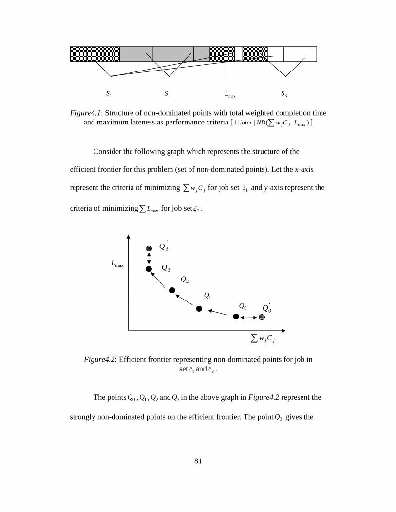
81

1S 2S maxL 3S

Figure4.1: Structure of non-dominated points with total weighted completion time and maximum lateness as performance criteria [ ),(||1 maxLCwNDinter jj∑ ]

Consider the following graph which represents the structure of the

efficient frontier for this problem (set of non-dominated points). Let the x-axis

represent the criteria of minimizing ∑ jj Cw for job set 1ξ and y-axis represent the

criteria of minimizing∑ maxL for job set 2ξ .

Figure4.2: Efficient frontier representing non-dominated points for job in set 1ξ and 2ξ .

The points 0Q , 1Q , 2Q and 3Q in the above graph in Figure4.2 represent the

strongly non-dominated points on the efficient frontier. The point 3Q gives the

maxL

∑ jj Cw

0Q

2Q

1Q '0Q

'3Q

3Q

82

best value of total weighted completion time for jobs in set1ξ . Similarly 0Q gives

the best value of maximum lateness of jobs from set2ξ . The point '0Q is the point

which is weakly non-dominated by the jobs in set1ξ and point '3Q is weakly non-

dominated by the jobs in set2ξ . The strongly non-dominated point 0Q can be

represented by minmax,||1 YLCwinter jj =∑ , where minY is the best value of maximum

lateness obtained by solving ∑ max||1 L for second set without interference.

Similarly strongly non-dominated point 3Q can be represented by

maxmin ,||1 LKCwinter jj =∑ , where minK is the minimum total weighted completion

time obtained by solving ∑ jj Cw||1 for first set without interference. Note that

only the point maxmin ,||1 LKCwinter jj =∑ is polynomially solvable. We can get this

point by scheduling all the jobs in set1ξ first by WSPT order followed by all the

jobs in set 2ξ in EDD order.

4. Forward WSPT-EDD Heuristic

The Forward WSPT–EDD algorithm can be summarized by the

following steps, where we start from the initial point

minmax,||1 YLCwinter jj =∑ (i.e. 0Q ) and then determine the next point by allowing

increments in maxL value until we reach point maxmin ,||1 LKCwinter jj =∑ (i.e. 3Q ):

Step1: Arrange the jobs in 2ξ in EDD order starting at time zero.

83

Step2: Find the job j* from 2ξ which has the maxL value. This job will divide the

jobs in the second set (2ξ ) into 2S and 3S . Also if there is a tie between the jobs for

the maxL , pick the job with minimum due date as the j* job.

Step3: All the jobs in 2S will occur in a block with the last job being j* . The jobs

from set 2ξ that are scheduled after this job j* (jobs in 3S ) can be moved further

in the time horizon to take advantage of the slack with respect to their completion

time and maxL value. This will create an opportunity for improvement in the

performance criterion of jobs in 1S without impacting the maxL value.

Note that the all jobs in set 3S will not have the same slack with respect to

their completion time and the current maxL value. The following algorithm can be

used to determine the slack in the lateness (Lj ) and the maxL value for the jobs in

set 3S and then update the Cj values. At this step, jobs in 2ξ are already arranged

in the EDD order with n2 being the last job.

Initialize )(2max nLLk −=

For j = n2,….., 3, 2, 1

If j = j*, STOP.

Else, )](,min[ max jLLkk −=

kCC jj +=

End

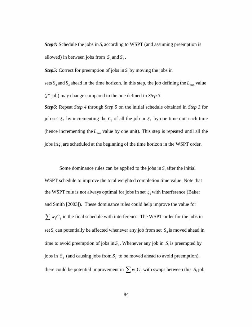
84

Step4: Schedule the jobs in1S according to WSPT (and assuming preemption is

allowed) in between jobs from 2S and 3S .

Step5: Correct for preemption of jobs in1S by moving the jobs in

sets 2S and 3S ahead in the time horizon. In this step, the job defining themaxL value

(j* job) may change compared to the one defined in Step 3.

Step6: Repeat Step 4 through Step 5 on the initial schedule obtained in Step 3 for

job set 2ξ by incrementing the Cj of all the job in 2ξ by one time unit each time

(hence incrementing themaxL value by one unit). This step is repeated until all the

jobs in 1ξ are scheduled at the beginning of the time horizon in the WSPT order.

Some dominance rules can be applied to the jobs in1S after the initial

WSPT schedule to improve the total weighted completion time value. Note that

the WSPT rule is not always optimal for jobs in set 1ξ with interference (Baker

and Smith [2003]). These dominance rules could help improve the value for

∑ jjCw in the final schedule with interference. The WSPT order for the jobs in

set 1S can potentially be affected whenever any job from set 3S is moved ahead in

time to avoid preemption of jobs in1S . Whenever any job in 1S is preempted by

jobs in 3S (and causing jobs from3S to be moved ahead to avoid preemption),

there could be potential improvement in ∑ jjCw with swaps between this 1S job

85

and the subsequent 1S job in the schedule. However this dominance rule could

become very complicated depending on how many jobs are alternating between

set 1S and set 3S . Also, we did not notice any significant improvement in the

solution quality after applying some simple dominance criteria.

4.1. Example

Consider an example with 5 jobs in each set of jobs 1ξ and 2ξ being

represented by1jp and 2

jp , respectively. For simplicity before numbering the jobs,

jobs in set1ξ are arranged in WSPT order while the jobs in set2ξ are arranged in

EDD order. The final sequence at any non-dominated point is divided into 3 sets:

1S which includes all jobs from1ξ arranged in WSPT order, 2S which includes

maxL job (or job j* ) and all the jobs before maxL job from set 2ξ and 3S which

includes all the jobs after maxL job from set 2ξ .

For set 1ξ : 11p =1, 1

2p =5, 13p =5, 1

4p =3, 15p =2

11w =4, 1

2w =6, 13w =5, 1

4w =2, 15w =1

For set 2ξ : 21p =3, 2

2p =6, 23p =4, 2

4p =5, 25p =3

21d =5, 2

2d =8, 23d =10, 2

4d =17, 25d =24

86

The value of ∑ jj Cw for problem ∑ jj Cw||1 is 139, while maxL for

problem max||1 L is 3. The maxL job j* is 3 from set 2ξ . After determining j* in the

iteration (1), the set 2ξ is divided into 2S = {1, 2, 3} and 3S = {4, 5}. We use the

logic in step3 to update the completion time of the jobs in3S . Hence the initial 2jC

values {3, 9, 13, 18, 21} are updated to {3, 9, 13, 20, 27}. Jobs in set1ξ are

arranged in WSPT order with preemption and then the jobs in the set 2ξ are pulled

ahead to avoid preemption for jobs in1ξ , which creates a non-preemptive and

feasible schedule. This results in point 0Q (467, 3), which provides the best

possible value for jobs in set2ξ .

1 2 3 4 5 6 7 8 9 10 11 12 13 14 15 16 17 18 19 20 21 22 23 24 25 26 27 28 29 30 31 32 33 34 35 36 37 381 2 3 4 51 2 3 1 4 2 5 3 4 5

Figure4.3(a): In the first row jobs in 1ξ are allowed to be preempted. In the second row jobs in set 2ξ are pulled ahead to avoid preemption of jobs in set1ξ which

creates a non-preemptive and feasible schedule. Note that the completion time of the jobs in 1ξ remains the same.

In iteration (2), all the jobs in2ξ are moved by one time unit and then the

jobs in set1ξ are arranged in WSPT with preemption. Next, the jobs in the set

2ξ are pulled ahead to avoid preemption for jobs in1ξ . This gives the non-

dominated point 1Q (415, 4).

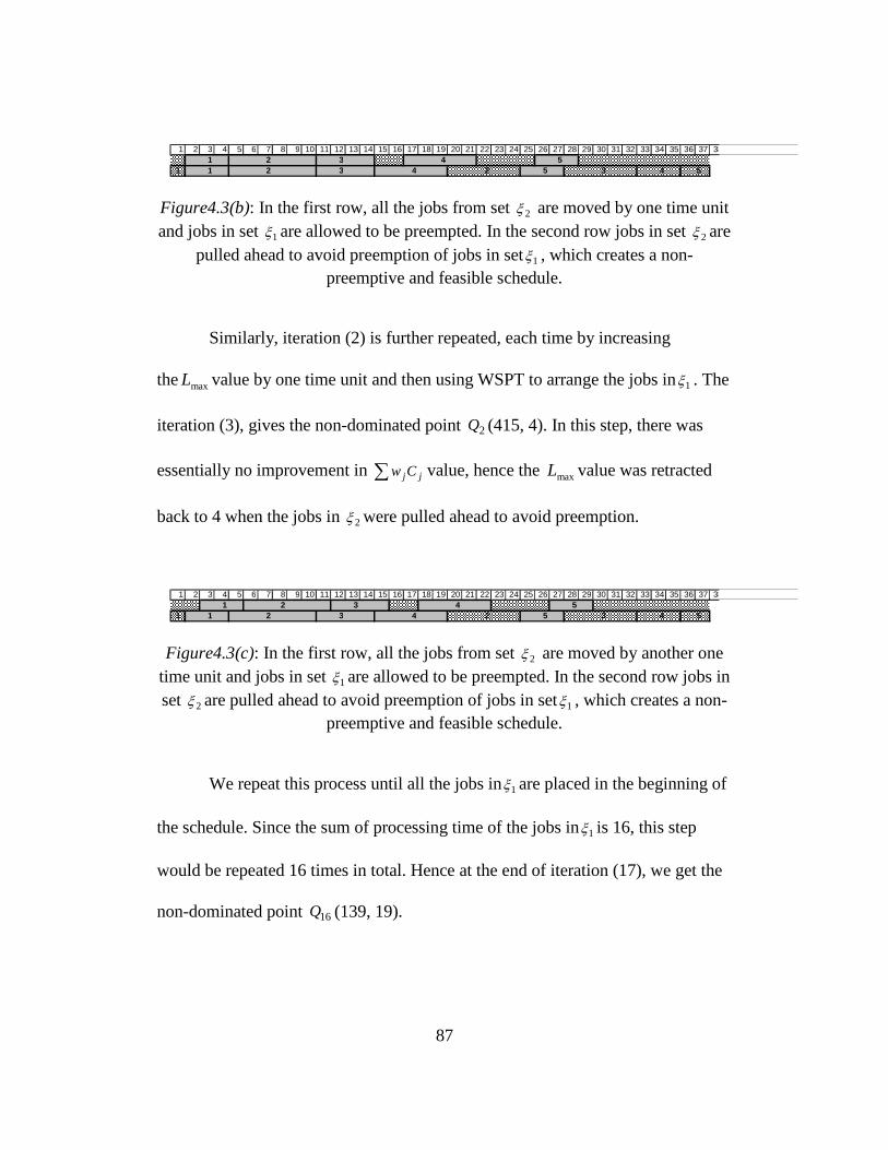
87

1 2 3 4 5 6 7 8 9 10 11 12 13 14 15 16 17 18 19 20 21 22 23 24 25 26 27 28 29 30 31 32 33 34 35 36 37 381 2 3 4 5

1 1 2 3 4 2 5 3 4 5

Figure4.3(b): In the first row, all the jobs from set 2ξ are moved by one time unit and jobs in set 1ξ are allowed to be preempted. In the second row jobs in set 2ξ are

pulled ahead to avoid preemption of jobs in set1ξ , which creates a non-preemptive and feasible schedule.

Similarly, iteration (2) is further repeated, each time by increasing

the maxL value by one time unit and then using WSPT to arrange the jobs in 1ξ . The

iteration (3), gives the non-dominated point 2Q (415, 4). In this step, there was

essentially no improvement in ∑ jj Cw value, hence the maxL value was retracted

back to 4 when the jobs in 2ξ were pulled ahead to avoid preemption.

1 2 3 4 5 6 7 8 9 10 11 12 13 14 15 16 17 18 19 20 21 22 23 24 25 26 27 28 29 30 31 32 33 34 35 36 37 381 2 3 4 5

1 1 2 3 4 2 5 3 4 5

Figure4.3(c): In the first row, all the jobs from set 2ξ are moved by another one time unit and jobs in set 1ξ are allowed to be preempted. In the second row jobs in set 2ξ are pulled ahead to avoid preemption of jobs in set1ξ , which creates a non-

preemptive and feasible schedule.

We repeat this process until all the jobs in1ξ are placed in the beginning of

the schedule. Since the sum of processing time of the jobs in 1ξ is 16, this step

would be repeated 16 times in total. Hence at the end of iteration (17), we get the

non-dominated point 16Q (139, 19).

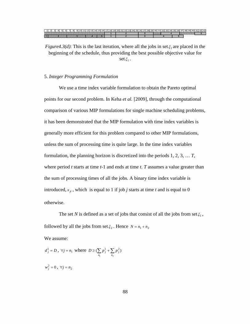
88

1 2 3 4 5 6 7 8 9 10 11 12 13 14 15 16 17 18 19 20 21 22 23 24 25 26 27 28 29 30 31 32 33 34 35 36 37 38 39 40 41 42 431 2 3 4 5

1 2 3 4 5 1 2 3 4 5

Figure4.3(d): This is the last iteration, where all the jobs in set1ξ are placed in the beginning of the schedule, thus providing the best possible objective value for

set 1ξ .

5. Integer Programming Formulation

We use a time index variable formulation to obtain the Pareto optimal

points for our second problem. In Keha et al. [2009], through the computational

comparison of various MIP formulations for single machine scheduling problems,

it has been demonstrated that the MIP formulation with time index variables is

generally more efficient for this problem compared to other MIP formulations,

unless the sum of processing time is quite large. In the time index variables

formulation, the planning horizon is discretized into the periods 1, 2, 3, … T,

where period t starts at time t-1 and ends at time t. T assumes a value greater than

the sum of processing times of all the jobs. A binary time index variable is

introduced, jtx , which is equal to 1 if job j starts at time t and is equal to 0

otherwise.

The set N is defined as a set of jobs that consist of all the jobs from set 1ξ ,

followed by all the jobs from set2ξ . Hence 21 nnN +=

We assume:

Dd j =1 , 1nj =∀ where )(

21

21 ∑∑ +≥n

jn

j ppD

02 =jw , 2nj =∀

89

Constraint 1: Each job can start only at exactly one particular time

∑+−

=

=1

1

1jpT

tjtx Nj ∈∀ (1.1)

Constraint 2: At any given time at most one job can be processed

∑ ∑= +−=

≤n

j

t

ptsjsj

x,1 )1,0max(

1 Tt ,........,1= , (1.2)

Constraint 3: Integrality constraints

}1,0{∈jtx TtNj ,......,1; =∈∀ . (1.3)

Constraint 4: Limiting the LMAX value to obtain a Pareto-optimal point

MAXj

pT

tjtj Ld- xpt

j

≤+−∑+−

=

1

1

)1(

Nj ∈∀

(1.4)

Alternately, we can introduce a slack variable in Eq (1.4) and convert the

inequality to an equality. The slack variable then could be part of objective

function.

90

The objective function is defined as

Minimize∑ ∑=

+−

=

+−nj jt

pT

tjj xptw

j

1

1

1

)1(

To obtain the efficient frontier, we vary the LMAX value in (1.4) from the

least value that is possible by solving the MAXL||1 for set 2ξ alone (using EDD)

and the maximum value at which the total weighted tardiness for set 1ξ has the

least possible value. The above MIP formulation is similar to the problem of a

single machine with the objective of minimizing total weighted completion time

with deadlines. This problem is dealt with a separate branch and bound algorithm

by Posner [1985] as well as by T’Kindt et al. [2004].

6. Computational Experiments

We compare the computational efficiency and solution quality of our

heuristic for the problem with the optimal solutions by generating 120 problem

instances for various numbers of jobs in each set. For the symmetric scenarios, we

consider cases with 20, 30, 40 and 50 jobs in each set1ξ and 2ξ and generate

twenty problem instances for each case. Further, for the asymmetric scenario, we

consider cases with 10 and 30 jobs in set1ξ and 2ξ . We select integer processing

time numbers for both sets of jobs from ~ U [1, 20]. The due date,jd , of job j is

an integer generated from the uniform distribution [P (L-R/2), P (L+R/2)], where

P = 0.5 P1 + P2 (P1 is the sum of processing time in of jobs in set1ξ and P2 is the

91

sum of processing time of jobs in set2ξ ) and the two parameters L and R are

relative measures of the location and range of the distribution, respectively. This

particular methodology of generating the due date ranges is adopted from Abdul-

Razaq et al. [1990] and has been used in other papers as well (Keha et al. [2009]).

We choose L ∈ {0.5, 0.7} and R ∈ {0.4, 0.8} to generate four different ranges of

due dates: [0.3 P, 0.7P], [0.1 P, 0.9P], [0.5 P, 0.9P] and [0.3 P, 1.1P]; and

generate five problem instances for each range, hence generating twenty problem

instances in total for each number of jobs. The weights of the jobs jw are selected

from ~ U [1, 10]. To test the computational efficiency we have selected up to 100

job problem instances (50 jobs in each set).

Before we discuss the results, note that the number of non-dominated

solutions can be very different depending on the pair of objectives considered. For

example, since both total weighted completion time and maximum lateness can

potentially have very large ranges, the number of non-dominated points can be

significantly high. Presenting a very large number of points can be confusing to

the decision maker. Therefore for this problem we restrict our comparisons to the

number of supported non-dominated points. The set of supported non-dominated

points is a subset of the set of all non-dominated points and can be obtained by

optimally solving all possible convex combinations of the two objectives. The

smaller subset of supported points that are initially presented can be used by the

decision-maker, if necessary, to guide the search for specific non-supported points

that lie within certain ranges.

92

The heuristic is coded using MATLAB 2009b. The MIP formulation for

the problem is modeled using AMPL (Fourer et al. [1993]) and solved using

CPLEX 12.3. The experiments were run on a windows machine with 1.66 GHz

processor and 2.5GB memory.

7. Results

To test the performance of the forward WSPT-EDD heuristic for our

second problem ),(||1 maxLCwNDinter jj∑ , we compare the set of supported points

for each problem instance with the results from the time index MIP formulation of

the problem. Since maxL could potentially have a wide range of values, the total

number of non-dominated points for this problem can be large. Hence we restrict

our computational comparison with the solutions from the MIP to only the

supported points obtained from the heuristic. We find that even the set of

supported points can be fairly large (given the number of jobs in each set), hence

a decision maker might not be interested in all the non-dominated points but more

in the points that lie on the efficient frontier (i.e. all the supported points).

After obtaining the set of all near non-dominated points from the forward

WSPT-EDD heuristic, we make use of the equation: ∑−+ jj CwL )1(max αα to filter

all the supported points. Supported points are those that lie on the efficient

frontier (and are therefore optimal under some convex or linear combination of

the two objectives), while non-supported points are non-dominated points that do

93

not lie on the efficient frontier. The value of α is varied between 0.005 and 0.995

in an increment of 0.005. Also, since the scale of these two objective values are

different, we normalize this equation by dividing the maxL and ∑ jjCw values of all

points in the solution set by minY and minK , respectively. minY is the best value of

maximum lateness obtained at point minmax,||1 YLwjCinter j =∑ and minK is the best

value of total weighted completion time obtained at points

maxmin ,||1 LKwjCinter j =∑ . Thus, this approach yields a set of near non dominated

points generated by our heuristic that lie on the efficient frontier (supported

points).

Table4.1 summarizes the comparison of the average computational time of

the Forward WSPT-EDD heuristic with the run time of the MIP formulations

(with a 1 hour time limit for each solution point) to generate the Pareto optimal

solutions sets (or 1 hour time limited best integer solution). The run time to

generate all the non-dominated points as well as to reduce the solution set to only

the supported points for any problem instance (column 4) by the Forward WSPT-

EDD heuristic was less than 1 second. This includes 120 problem instances with

different number of jobs, as reflected in the Table4.1. On the other hand the MIP

took a fair amount of time to solve for the set of supported points for each

problem instance (column 5). For lower number of jobs (20 jobs in each set), the

average MIP run time for all 20 instances was in the range of 2 minutes to 15

minutes, while for the larger number of jobs (50 jobs in each set), the average

MIP run time for all 20 instances was in the range of 3 hours to 20 hours. There

94

was also an increase in the number of supported points (column 6) with a larger

number of jobs in the problem instance. Further with an increase in the number of

jobs in each set, there was an increase in the problem instances where the solution

obtained from the MIP was limited by the 1 hour computation time (column 7).

Note that the goal of this paper is not just to compare the run time of the

heuristics with the MIP formulations, but to highlight the fact that the

performance of this heuristic is so close to the optimal solutions (gaps being less

than 0.50%, discussed in the subsequent paragraph) that there is hardly any need

to run the MIP or any improved branch and bound algorithms for the problem.

Posner [1985] and T’Kindt et al. [2004] have suggested improved branch and

bound algorithms for this particular problem with improvements in the run time

over the MIP formulations. But even these improvements can not yield a run time

which is less then 1 second across multiple problem instances with up to 100 jobs.

Table4.2 summarizes the solution quality of the Forward WSPT-EDD

heuristic with the solutions obtained from the time limited MIP solutions across

various problem instances. As expected, the average number of supported points

generated by the time limited MIP (column 4) as well as the average number of

non Pareto optimal points (column 5) increases with an increase in the number of

jobs in each set. The average percentage gap between the supported points that are

non Pareto optimal for each instance (column 6) obtained from the time limited

MIP and the Forward WSPT-EDD heuristic is under 0.5% (for symmetric as well

as asymmetric problem instances). In other words, for all non-Pareto supported

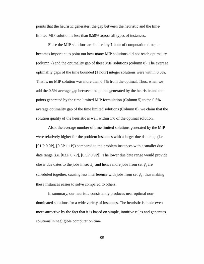
95

points that the heuristic generates, the gap between the heuristic and the time-

limited MIP solution is less than 0.50% across all types of instances.

Since the MIP solutions are limited by 1 hour of computation time, it

becomes important to point out how many MIP solutions did not reach optimality

(column 7) and the optimality gap of these MIP solutions (column 8). The average

optimality gaps of the time bounded (1 hour) integer solutions were within 0.5%.

That is, no MIP solution was more than 0.5% from the optimal. Thus, when we

add the 0.5% average gap between the points generated by the heuristic and the

points generated by the time limited MIP formulation (Column 5) to the 0.5%

average optimality gap of the time limited solutions (Column 8), we claim that the

solution quality of the heuristic is well within 1% of the optimal solution.

Also, the average number of time limited solutions generated by the MIP

were relatively higher for the problem instances with a larger due date rage (i.e.

[01.P 0.9P], [0.3P 1.1P]) compared to the problem instances with a smaller due

date range (i.e. [03.P 0.7P], [0.5P 0.9P]). The lower due date range would provide

closer due dates to the jobs in set 2ξ and hence more jobs from set 2ξ are

scheduled together, causing less interference with jobs from set 1ξ , thus making

these instances easier to solve compared to others.

In summary, our heuristic consistently produces near optimal non-

dominated solutions for a wide variety of instances. The heuristic is made even

more attractive by the fact that it is based on simple, intuitive rules and generates

solutions in negligible computation time.

96

8. Conclusion and Future Research

The proposed polynomial heuristic does a good job of providing a set of

nearly supported non dominated points; the average gap is less than 1% compared

to the optimal solution. The computational experiment could be extended to see

the effect of the increased run time with a larger number of jobs with the pseudo-

polynomial algorithm. It can be clearly seen that the WSPT-EDD heuristic for

),(||1 maxLCwNDinter jj∑ performs quite well and will be useful in solving job sets

each with a larger number of jobs e.g. 200 or higher. The structure of the problem

explored in this paper may be useful in developing branch and bound algorithms

similar to ones proposed by T’Kindt et al. [2004] and Posner [1985], specifically

for the interfering job sets. A similar approach could be adopted to solve other

interfering job set problems with different performance criteria; even problems

which have been classified as NP-hard.

We further intend to carry our more computational experiments as well as

explore the structure of the single machine problems with two interfering job sets

with the criterion of total weighted completion time and number of tardy jobs

[ ),(||1 ∑∑ jjj UCwNDinter ] as well as similar criterion in the parallel machine

environment. Further it will be interesting to see if Moore’s rule will still hold for

on time jobs or jobs with the criteria of minimizing number of tardy jobs when

interfering with another job set that has the criterion to minimize total weighted

completion time. It will be interesting to see how we can make use of the various

97

polynomial time algorithms (like EDD, Moore’s rule, SPT, WSPT, etc) in the

parallel machine environment and develop similar heuristics.

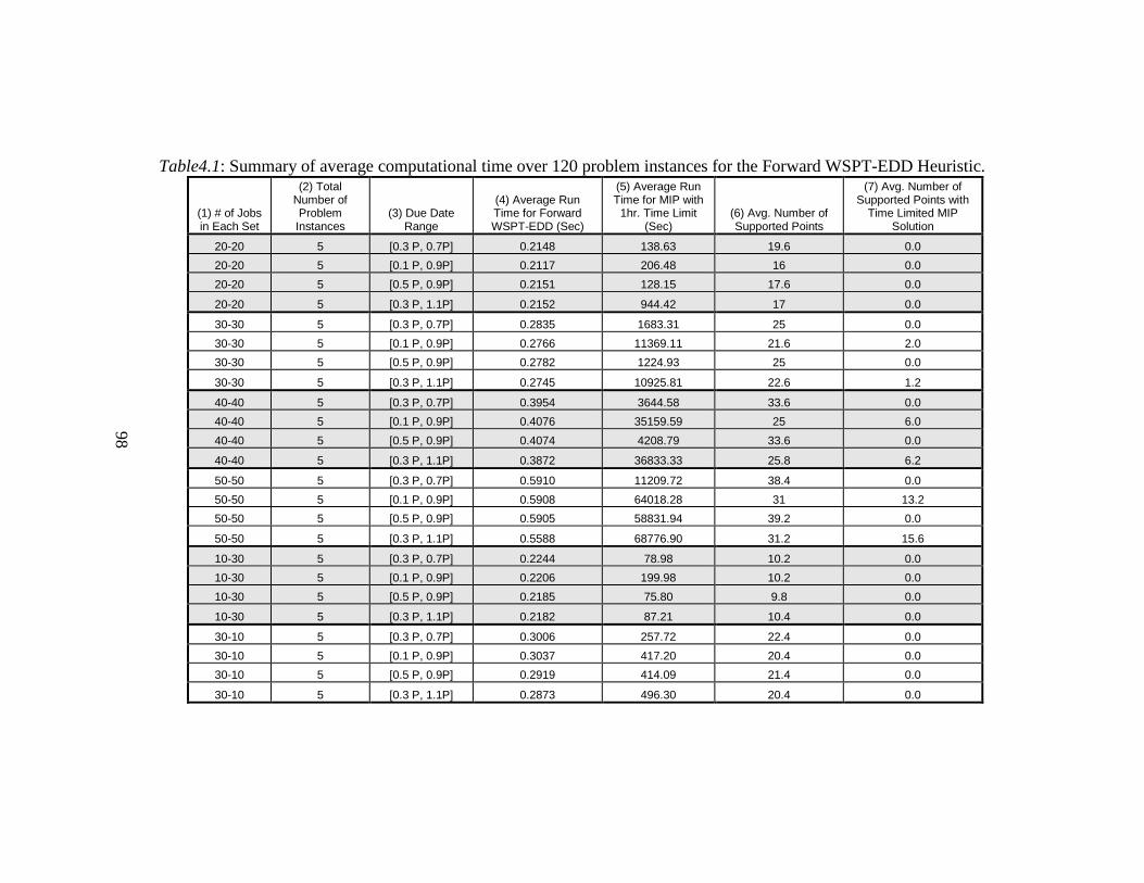
98

Table4.1: Summary of average computational time over 120 problem instances for the Forward WSPT-EDD Heuristic.

98

(1) # of Jobs in Each Set


(3) Due Date Range

(4) Average Run Time for Forward WSPT-EDD (Sec)

(5) Average Run Time for MIP with

1hr. Time Limit (Sec)

(6) Avg. Number of Supported Points

(7) Avg. Number of Supported Points with

Time Limited MIP Solution

20-20 5 [0.3 P, 0.7P] 0.2148 138.63 19.6 0.0

20-20 5 [0.1 P, 0.9P] 0.2117 206.48 16 0.0

20-20 5 [0.5 P, 0.9P] 0.2151 128.15 17.6 0.0

20-20 5 [0.3 P, 1.1P] 0.2152 944.42 17 0.0

30-30 5 [0.3 P, 0.7P] 0.2835 1683.31 25 0.0

30-30 5 [0.1 P, 0.9P] 0.2766 11369.11 21.6 2.0

30-30 5 [0.5 P, 0.9P] 0.2782 1224.93 25 0.0

30-30 5 [0.3 P, 1.1P] 0.2745 10925.81 22.6 1.2

40-40 5 [0.3 P, 0.7P] 0.3954 3644.58 33.6 0.0

40-40 5 [0.1 P, 0.9P] 0.4076 35159.59 25 6.0

40-40 5 [0.5 P, 0.9P] 0.4074 4208.79 33.6 0.0

40-40 5 [0.3 P, 1.1P] 0.3872 36833.33 25.8 6.2

50-50 5 [0.3 P, 0.7P] 0.5910 11209.72 38.4 0.0

50-50 5 [0.1 P, 0.9P] 0.5908 64018.28 31 13.2

50-50 5 [0.5 P, 0.9P] 0.5905 58831.94 39.2 0.0

50-50 5 [0.3 P, 1.1P] 0.5588 68776.90 31.2 15.6

10-30 5 [0.3 P, 0.7P] 0.2244 78.98 10.2 0.0

10-30 5 [0.1 P, 0.9P] 0.2206 199.98 10.2 0.0

10-30 5 [0.5 P, 0.9P] 0.2185 75.80 9.8 0.0

10-30 5 [0.3 P, 1.1P] 0.2182 87.21 10.4 0.0

30-10 5 [0.3 P, 0.7P] 0.3006 257.72 22.4 0.0

30-10 5 [0.1 P, 0.9P] 0.3037 417.20 20.4 0.0

30-10 5 [0.5 P, 0.9P] 0.2919 414.09 21.4 0.0

30-10 5 [0.3 P, 1.1P] 0.2873 496.30 20.4 0.0

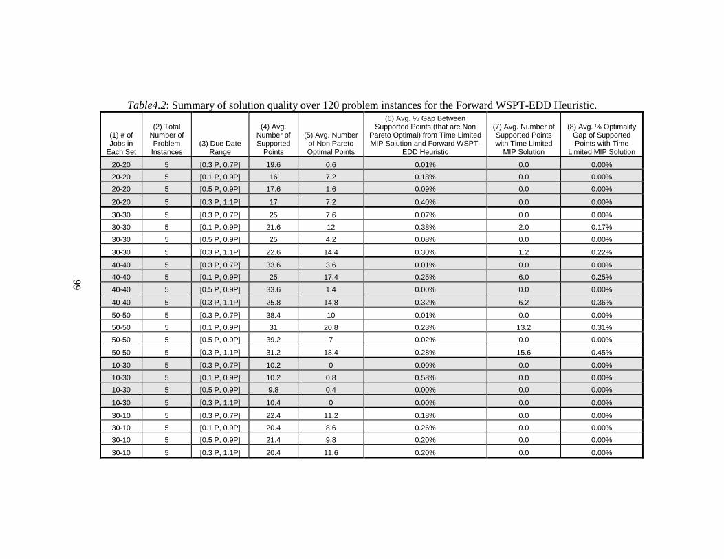
99

Table4.2: Summary of solution quality over 120 problem instances for the Forward WSPT-EDD Heuristic.

99

(1) # of Jobs in

Each Set


(3) Due Date Range

(4) Avg. Number of Supported

Points

(5) Avg. Number of Non Pareto Optimal Points

(6) Avg. % Gap Between Supported Points (that are Non

Pareto Optimal) from Time Limited MIP Solution and Forward WSPT-

EDD Heuristic

(7) Avg. Number of Supported Points with Time Limited

MIP Solution

(8) Avg. % Optimality Gap of Supported Points with Time

Limited MIP Solution

20-20 5 [0.3 P, 0.7P] 19.6 0.6 0.01% 0.0 0.00%

20-20 5 [0.1 P, 0.9P] 16 7.2 0.18% 0.0 0.00%

20-20 5 [0.5 P, 0.9P] 17.6 1.6 0.09% 0.0 0.00%

20-20 5 [0.3 P, 1.1P] 17 7.2 0.40% 0.0 0.00%

30-30 5 [0.3 P, 0.7P] 25 7.6 0.07% 0.0 0.00%

30-30 5 [0.1 P, 0.9P] 21.6 12 0.38% 2.0 0.17%

30-30 5 [0.5 P, 0.9P] 25 4.2 0.08% 0.0 0.00%

30-30 5 [0.3 P, 1.1P] 22.6 14.4 0.30% 1.2 0.22%

40-40 5 [0.3 P, 0.7P] 33.6 3.6 0.01% 0.0 0.00%

40-40 5 [0.1 P, 0.9P] 25 17.4 0.25% 6.0 0.25%

40-40 5 [0.5 P, 0.9P] 33.6 1.4 0.00% 0.0 0.00%

40-40 5 [0.3 P, 1.1P] 25.8 14.8 0.32% 6.2 0.36%

50-50 5 [0.3 P, 0.7P] 38.4 10 0.01% 0.0 0.00%

50-50 5 [0.1 P, 0.9P] 31 20.8 0.23% 13.2 0.31%

50-50 5 [0.5 P, 0.9P] 39.2 7 0.02% 0.0 0.00%

50-50 5 [0.3 P, 1.1P] 31.2 18.4 0.28% 15.6 0.45%

10-30 5 [0.3 P, 0.7P] 10.2 0 0.00% 0.0 0.00%

10-30 5 [0.1 P, 0.9P] 10.2 0.8 0.58% 0.0 0.00%

10-30 5 [0.5 P, 0.9P] 9.8 0.4 0.00% 0.0 0.00%

10-30 5 [0.3 P, 1.1P] 10.4 0 0.00% 0.0 0.00%

30-10 5 [0.3 P, 0.7P] 22.4 11.2 0.18% 0.0 0.00%

30-10 5 [0.1 P, 0.9P] 20.4 8.6 0.26% 0.0 0.00%

30-10 5 [0.5 P, 0.9P] 21.4 9.8 0.20% 0.0 0.00%

30-10 5 [0.3 P, 1.1P] 20.4 11.6 0.20% 0.0 0.00%

100

References

1. Abdul-Razaq, T. S., Potts, C. N., & Van Wassenhove, L. N. (1990). A survey of algorithms for the single machine total weighted tardiness scheduling problem. Discrete Applied Mathematics, 26, 235-253 2. Agnetis, A., Mirchandani, P. B., Pacciarelli, D. & Pacifici, A. (2004). Scheduling problems with two completing agents. Operations Research, 52(2), 229-242. 3. Baker, K. R. & Smith, J. C. (2003). A multiple criterion model for machine scheduling. Journal of Scheduling, 6, 7-16. 4. Balasubramanian H., Fowler J., Keha A. & Pfund M. (2009). Scheduling interfering job sets on parallel machines. European Journal of Operational Research, 199(1), 55-67. 5. Cheng, T.C.E., Ng, C.T. & Yuan, J.J. (2006). Multi-agent scheduling on a single machine to minimize total weighted number of tardy jobs. Theoretical Computer Science, 362, 273-281. 6. Fourer, R.D., Gay, D. M. & Kernighan, B. W. (1993). AMPL: A modeling language for mathematical programming. Boyd & Fraser Publishing Company. 7. Jackson, J. R. (1955). Scheduling a production line to minimize maximum tardiness. Management Science Research Project, (Research Report 43) University of California, Los Angles. 8. Keha, A., Khowala, K. & Fowler, J. (2009). Mixed integer programming formulations for the single machine scheduling problems. Computers & Industrial Engineering, 56, 357-367. 9. Khowala, K., Fowler, J., Keha, A. & Balasubramanian, H. (2009). Single machine scheduling with interfering job sets. Proceedings of the Multidisciplinary International Scheduling: Theory and Applications Conference (MISTA 2009), 357-365. 10. Khowala, K., Fowler, J., Keha, A. & Balasubramanian, H. (2011). Single machine scheduling with interfering job sets to minimize total weighted completion time and maximum lateness. Proceedings of the Multidisciplinary International Scheduling: Theory and Applications Conference (MISTA 2011), 568-572.

101

11. Lee, W.-C., Chen, S.-K., Chen, C.-W. & Wu, C.-C. (2011). A two-machine flowshop problem with two agents. Computers & Operations Research, 38, 98-104. 12. Leung, J. Y.-T., Pinedo, M. & Wan, G. (2010). Competitive two-agent scheduling and its application. Operations Research, 58(2), 458-469. 13. Ng, C.T., Cheng, T.C.E. & Yuan, J.J. (2006). A note on the complexity of the problem of two agent scheduling on a single machine. Journal of Combinatorial Optimization, 12, 387-394. 14. Peha, J. (1995). Heterogeneous-criteria scheduling: minimizing weighted number of tardy jobs and weighted completion time. Journal of Computers and Operations Research, 22(10), 1089-1100. 15. Posner, M. E. (1985). Minimizing weighted completion times with deadlines. Operations Research, 33(3), 562-574. 16. T’Kindt, V., Croce, F. D. & Esswein, C. (2004). Revisiting branch and bound search strategies for machine scheduling problems. Journal of Scheduling, 7, 429-440. 17. T’Kindt, V., Billaut, J. C. & Scott, H. (2006). Multicriteria Scheduling: Theory, Models and Algorithms. Springer, 2nd edition. 18. Wan, G., Leung, J. Y.-T. & Pinedo, M. (2009). Competitive agent scheduling with Controllable Processing Times. Proceedings of the Multidisciplinary International Scheduling: Theory and Applications Conference (MISTA 2009), 514-522. 19. Wan, G., Vakati, S. R., Leung, J. Y.-T. & Pinedo M. (2010). Scheduling two agent with controllable processing times. European Journal of Operational Research, 205(3), 528-539.

102

Chapter 5

CONCLUSION AND FUTURE RESEARCH

In this first part of this dissertation we compared the computational

performance of four different formulations on single machine scheduling

problems with varying complexity. The performance of these formulations very

much depend on the objective function, number of jobs and the sum of the

processing times of all the jobs. The Time Index Formulation (F2) and the Linear

Ordering Formulation (F3) appear to be the most widely used formulations in the

integer programming and scheduling literature. The Assignment and Positional

Date Formulation (F4) appears to be the least widely used. The Completion Time

Formulation (F1) often appears in textbooks and other literature that simply

formulates/describes the problem (not the solution methodology) and it clearly

does not generally perform well in practice.

With F1 and F4, the LP relaxation is easy to solve and readily provides a

feasible solution. F2 and F3 have been preferred due to the fact that they generally

produce tighter bounds. However, we have found that the LP relaxation of these

formulations tends to be much more difficult to solve. This is particularly true for

F2 when P (sum of processing time of all the jobs) is large. This limits one’s

ability to explore recent advancement in IP methodology (such as branch and cut).

On the other hand, the LP relaxation of F4 can be solved relatively quickly, so

this MIP formulation offers more promise for these new advanced techniques. We

gave two simple families of inequalities that improved the bounds obtained from

103

the LP- relaxation for F4. There was noticeable improvement in terms of

achieving a better bound (LP relaxation) and a reduction in the optimality gap by

adding the new set of inequalities to F4 and removing the big-M constraint.

As future research, the MIP formulations can be compared with other

additional restrictions, such as precedence constraints, or for more complex

machine environments. F4 might be the choice of formulation for an expert in

integer programming because the LP relaxation of this formulation can be solved

faster and a larger number of nodes can be explored in a fixed amount of

computational time. This creates the potential to use recent advancements found

in the integer programming literature. Studying the polyhedral structure of this

formulation and using valid inequalities in a branch-and-cut algorithm would

certainly be interesting to study in the future.

We further looked at single machine bicriteria scheduling problems with

interfering job sets (with each set of job having its own criteria to optimize).

Using MIP formulations for this domain of problems could be difficult as well as

computationally challenging. We look at some of these problems and exploit their

structure to define heuristics which yield near optimal solutions without many

computational challenges.

The proposed polynomial heuristics do a good job of providing a near non

dominated solution set (or the set of supported points); the average gap is less

than 1% compared to the optimal solution. The computational experiment could

be extended to see the effect on run time with a larger number of jobs with the

pseudo-polynomial algorithm. It can be clearly seen that the SPT-EDD heuristic

104

for ),(||1 ∑∑ jj UCNDinter and the WSPT-EDD heuristic for

),(||1 maxLCwNDinter jj∑ perform quite well and will be useful in solving job sets

each with a larger number of jobs e.g. 200 or higher. The structure of the second

problem explored in this paper may be useful in developing branch and bound

algorithms similar to ones proposed by T’Kindt et al. [2004] and Posner [1985],

specifically for the interfering job sets. A similar approach could be adopted to

solve other interfering job set problems with different performance criteria; even

problems which have been classified as NP-hard. We further intend to perform

more computational experiments as well as explore the structure of the single

machine problems with two interfering job sets with the criterion of total

weighted completion time and number of tardy jobs [ ),(||1 ∑∑ jjj UCwNDinter ] as

well as similar criterion in the parallel machine environment. Further it will be

interesting to see if Moore’s rule will still hold for on time jobs or jobs with the

criteria of minimizing the number of tardy jobs when interfering with another job

set that has the criterion to minimize total weighted completion time. It will be

interesting to see how we can make use of the various polynomial time algorithms

(like EDD, Moore’s rule, SPT, WSPT, etc) in the parallel machine environment in

the development of similar heuristics.

105

REFERENCES

1. Abdul-Razaq, T. S., Potts, C. N., & Van Wassenhove, L. N. (1990). A survey of algorithms for the single machine total weighted tardiness scheduling problem. Discrete Applied Mathematics, 26, 235-253. 2. Agnetis, A., Mirchandani, P. B., Pacciarelli, D. & Pacifici, A. (2004). Scheduling problems with two completing agents. Operations Research, 52(2), 229-242. 3. Baker, K. R. & Smith, J. C. (2003). A multiple criterion model for machine scheduling. Journal of Scheduling, 6, 7-16. 4. Balas, E. (1985). On the facial structure of scheduling polyhedra. Mathematical Programming, 24, 179-218. 5. Balasubramanian H., Fowler J., Keha A. & Pfund M. (2009). Scheduling interfering job sets on parallel machines. European Journal of Operational Research, 199(1), 55-67. 6. Blazewicz, J., Dror, M., & Weglarz, J. (1991). Mathematical programming formulations for machine scheduling: A survey. European Journal of Operational Research, 51, 283-300. 7. Cheng, T.C.E., Ng, C.T. & Yuan, J.J. (2006). Multi-agent scheduling on a single machine to minimize total weighted number of tardy jobs. Theoretical Computer Science, 362, 273-281. 8. Chudak, F. A., & Hochbaum, D. S. (1999). A half-integral linear programming relaxation for scheduling precedence-constrained jobs on a single machine. Operations Research Letters, 25, 199-204. 9. Fourer, R.D., Gay, D. M. & Kernighan, B. W. (1993). AMPL: A modeling language for mathematical programming. Boyd & Fraser Publishing Company. 10. Dauzère-Pérès, S. (1997). An efficient formulation for minimizing the number of late jobs in single-machine scheduling. IEEE Symposium on Emerging Technologies & Factory Automation (ETFA), 442-445. 11. Dauzère-Pérès, S., & Sevaux, M. (2003). Using Lagrangean relaxation to minimize the weighted number of late jobs on a single machine. Naval Research Logistics, 50(3), 273-288.

106

12. Dyer, M. E., & Wolsey, L. A. (1990). Formulating the single machine sequencing problem with release dates as a mixed integer program. Discrete Applied Mathematics, 26, 255-270. 13. Graham, R. L., Lawler, E. L., Lenstra, J. K., & Rinnooy Kan, A. H. G. (1979). Optimization and approximation in deterministic sequencing and scheduling: a survey. Annals of Discrete Mathematics, 5, 287-326. 14. Hariri, A. M. A., & Potts, C. N. (1983). An algorithm for single machine sequencing with release dates to minimize total weighted completion time. Discrete Applied Mathematics, 5, 99-109. 15. Jackson, J. R. (1955). Scheduling a production line to minimize maximum tardiness. Management Science Research Project, (Research Report 43) University of California, Los Angles. 16. Jaszkiewicz, A. (2003). Evaluation of Multiple Objective Metaheuristics. Lecture Notes in Economics and Mathematical Systems, 535, 65-89. 17. Keha, A., Khowala, K. & Fowler, J. (2009). Mixed integer programming formulations for the single machine scheduling problems. Computers &Industrial Engineering, 56, 357-367. 18. Khowala, K., Keha, A. B., & Fowler, J. (2005). A comparison of different formulations for the non-preemptive single machine total weighted tardiness scheduling problem. The Second Multidisciplinary International Conference on Scheduling: Theory & Application (MISTA 2005), 643-651. 19. Khowala, K., Fowler, J., Keha, A. & Balasubramanian, H. (2009). Single machine scheduling with interfering job sets. Proceedings of the Multidisciplinary International Scheduling: Theory and Applications Conference (MISTA 2009), 357-365. 20. Khowala, K., Fowler, J., Keha, A. & Balasubramanian, H. (2011). Single machine scheduling with interfering job sets to minimize total weighted completion time and maximum lateness. Proceedings of the Multidisciplinary International Scheduling: Theory and Applications Conference (MISTA 2011), 568-572. 21. Kise, H., Ibaraki, T., & Mine, H. (1978). A solvable case of the one-machine scheduling problem with ready and due times. Operations Research, 26, 121-126.

107

22. Lasserre, J. B., & Queyranne, M. (1992). Generic scheduling polyhedral and a new mixed-integer formulation for single-machine scheduling. Proceedings of the Second IPCO Conference, Carnegie-Mellon University, Pittsburgh, 136-149. 23. Lawler, E. L. (1977). A ‘pseudopolynomial’ time algorithm for sequencing jobs to minimize total tardiness. Annals of Discrete Mathematics, 1, 331-342. 24. Lee, W.-C., Chen, S.-K., Chen, C.-W. & Wu, C.-C. (2011). A two-machine flowshop problem with two agents. Computers & Operations Research, 38, 98-104. 25. Lenstra, J. K., Rinnooy Kan, A. H. G., & Brucker, P. (1977). Complexity of machine scheduling problems. Annals of Discrete mathematics, 1, 343-362. 26. Leung, J. Y.-T., Pinedo, M. & Wan, G. (2010). Competitive two-agent scheduling and its application. Operations Research, 58(2), 458-469. 27. Moore, J. M. (1968). An n job, one machine sequencing algorithm for minimizing the number of late jobs. Management Science, 15, 102-109. 28. Nemhauser, G. L., & Savelsbergh, M. W. P. (1992). A cutting plane algorithm for the single machine scheduling problem with release times. Combinatorial Optimization: New Frontiers in the Theory and Practice (M. Akgül, H. Hamacher and S. Tufecki, eds.), NATO ASI Series F: Computer and Systems Sciences, Springer: Berlin, 82, 63-84. 29. Ng, C.T., Cheng, T.C.E. & Yuan, J.J. (2006). A note on the complexity of the problem of two agent scheduling on a single machine. Journal of Combinatorial Optimization, 12, 387-394. 30. Peha, J. (1995). Heterogeneous-criteria scheduling: minimizing weighted number of tardy jobs and weighted completion time. Journal of Computers and Operations Research, 22(10), 1089-1100. 31. Posner, M. E. (1985). Minimizing weighted completion times with deadlines. Operations Research, 33(3), 562-574. 32. Potts, C. N., & Van Wassenhove, L. N. (1983). An algorithm for single machine sequencing with deadlines to minimize total weighted completion time. European Journal of Operational Research, 12, 379-389. 33. Potts, C. N., & Van Wassenhove, L. N. (1982). A decomposition algorithm for the single machine, total tardiness problem. Operations Research Letters, 1, 177-181.

108

34. Queyranne, M., & Wang, Y. (1991). Single-machine scheduling polyhedra with precedence constraints. Mathematics of Operations Research, 16, 1-20. 35. Queyranne, M. (1993). Structure of a simple scheduling polyhedron. Mathematical Programming, 58, 263-285. 36. Queyranne, M. (2004). Personal Communication at INFORMS Annual Conference, Denver, October, 2004. 37. Queyranne, M., & Schulz, A. S. (1994). Polyhedral approaches to machine scheduling. Technical Report 408/1994, Department of Mathematics, Technical University of Berlin, Berlin, Germany. 38. Smith, W. E. (1956). Various optimizers for single stage production. Naval Research Logistics Quarterly, 3, 59-66. 39. Šorić, K. (2000). A cutting plane algorithm for a single machine scheduling problem. European Journal of Operational Research, 127, 383-393. 40. Sousa, J. P., & Wolsey, L. A. (1992). A time-indexed formulation of non-preemptive single-machine scheduling problems. Mathematical programming, 54, 353-367. 41. T’Kindt, V., Croce, F. D. & Esswein, C. (2004). Revisiting branch and bound search strategies for machine scheduling problems. Journal of Scheduling, 7, 429-440. 42. T’Kindt, V., Billaut, J. C. & Scott, H. (2006). Multicriteria Scheduling: Theory, Models and Algorithms. Springer, 2nd edition. 43. van den Akker, J.M., van Hoesel, C. P. M., & Savelsbergh, M.W.P. (1999). A Polyhedral approach to single machine scheduling problems. Mathematical Programming, 85, 541-572. 44. Wan, G., Leung, J. Y.-T. & Pinedo, M. (2009). Competitive agent scheduling with Controllable Processing Times. Proceedings of the Multidisciplinary International Scheduling: Theory and Applications Conference (MISTA 2009), 514-522. 45. Wan, G., Vakati, S. R., Leung, J. Y.-T. & Pinedo M. (2010). Scheduling two agent with controllable processing times. European Journal of Operational Research, 205(3), 528-539.

Documents

Single Machine Scheduling: Comparison of MIP … Machine Scheduling: Comparison of MIP Formulations and ... number of tardy jobs for the two sets of jobs is studied. A ... of this