MSRI, Berkeley, June 2004

Singularity Analysis: A Perspective

Philippe Flajolet

(Inria, France)

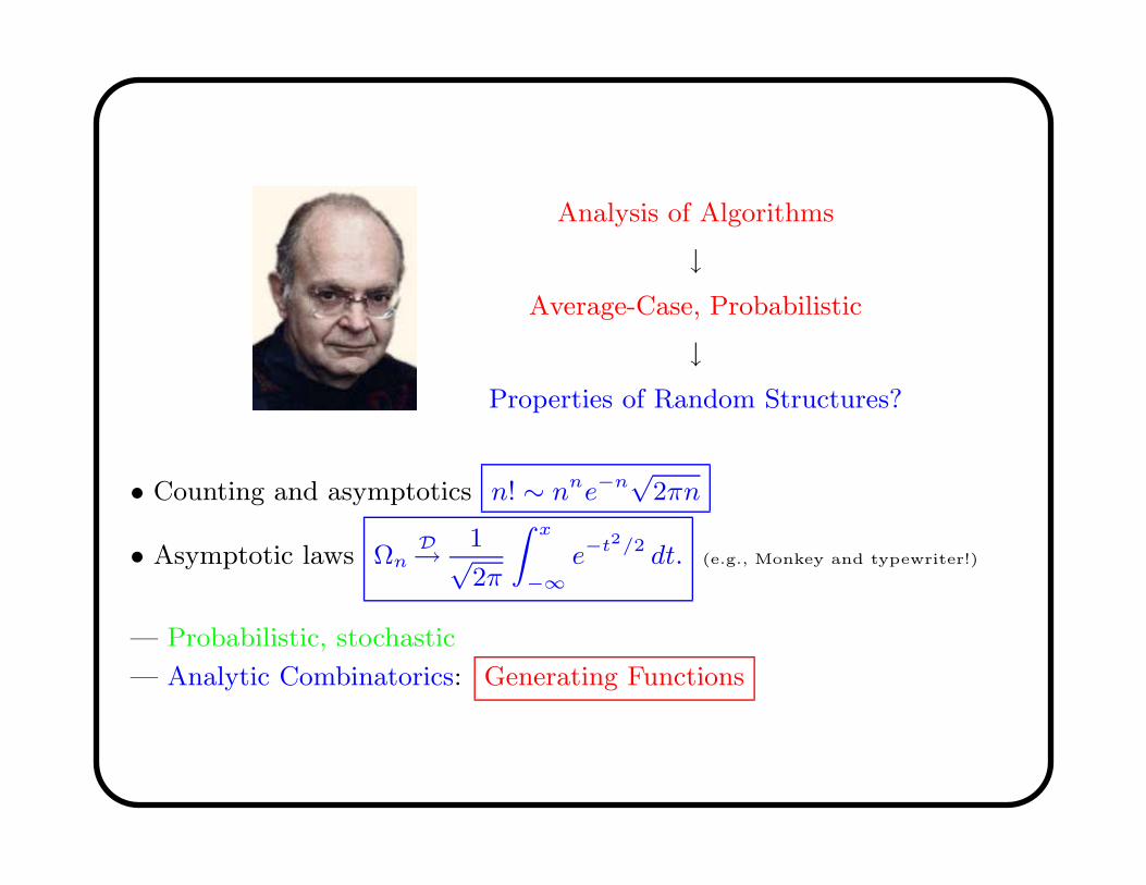
Analysis of Algorithms

↓Average-Case, Probabilistic

↓Properties of Random Structures?

• Counting and asymptotics n! ∼ nne−n√

2πn

• Asymptotic laws ΩnD→ 1√

2π

Z x

−∞e−t2/2 dt. (e.g., Monkey and typewriter!)

— Probabilistic, stochastic

— Analytic Combinatorics: Generating Functions

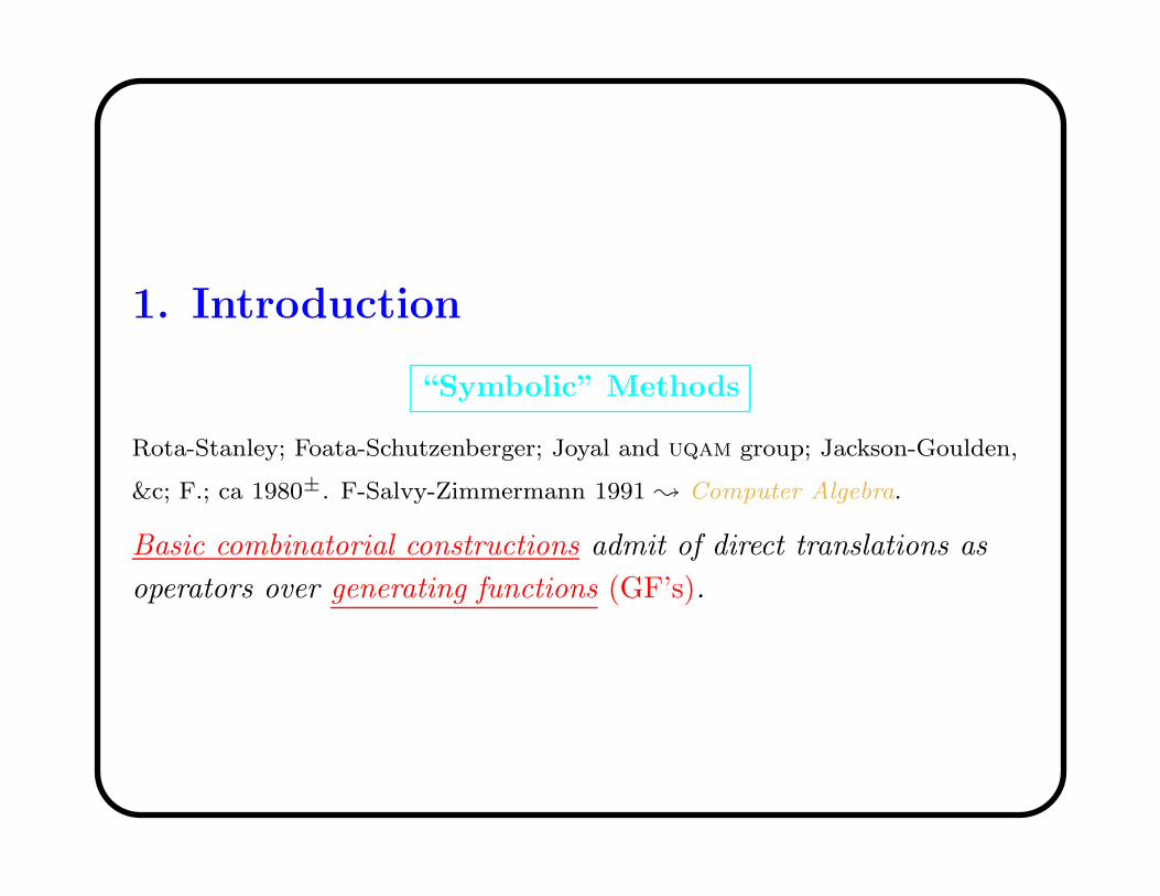
1. Introduction

“Symbolic” Methods

Rota-Stanley; Foata-Schutzenberger; Joyal and uqam group; Jackson-Goulden,

&c; F.; ca 1980±. F-Salvy-Zimmermann 1991 ; Computer Algebra.

Basic combinatorial constructions admit of direct translations as

operators over generating functions (GF’s).

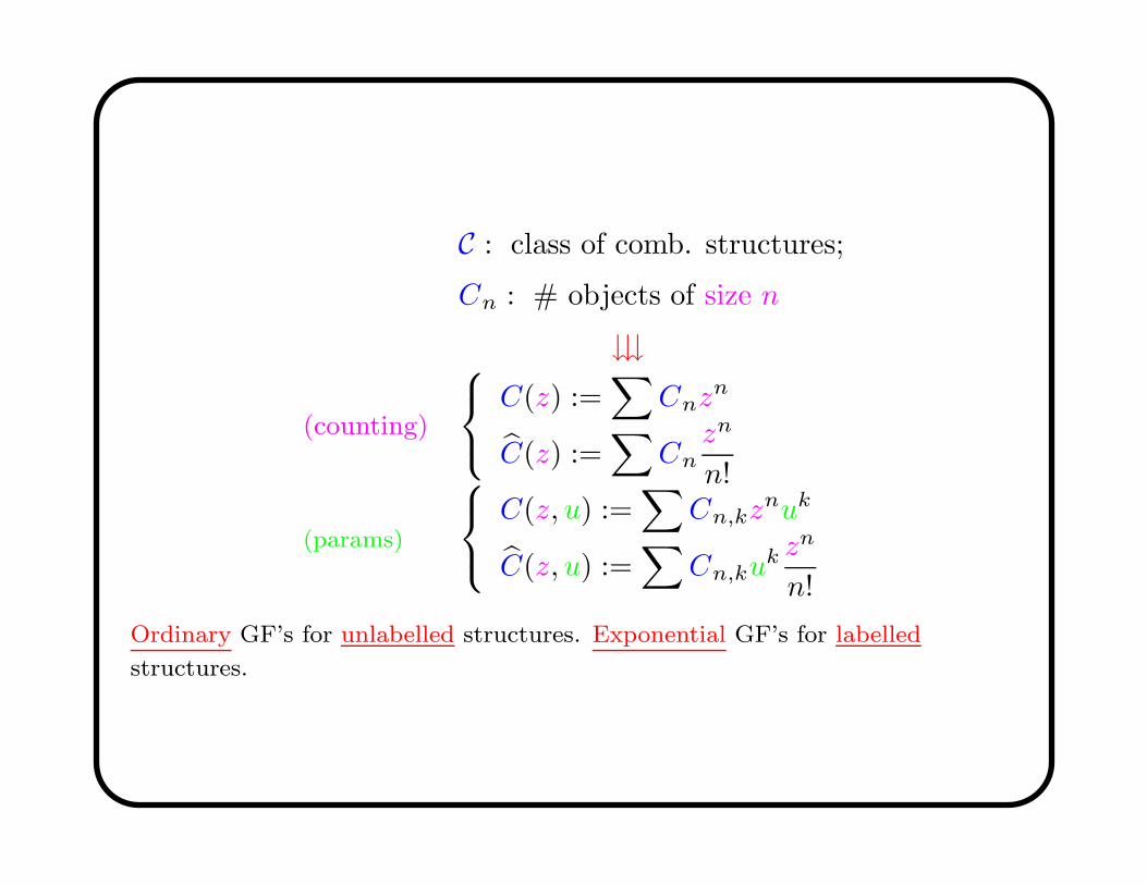
C : class of comb. structures;

Cn : # objects of size n

↓↓↓

(counting)

C(z) :=∑

Cnzn

C(z) :=∑

Cnzn

n!

(params)

C(z, u) :=∑

Cn,kznuk

C(z, u) :=∑

Cn,kuk zn

n!

Ordinary GF’s for unlabelled structures. Exponential GF’s for labelled

structures.

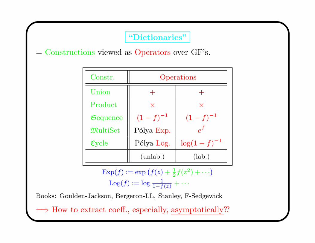
“Dictionaries”

= Constructions viewed as Operators over GF’s.

Constr. Operations

Union + +

Product × ×Sequence (1 − f)−1 (1 − f)−1

MultiSet Polya Exp. ef

Cycle Polya Log. log(1 − f)−1

(unlab.) (lab.)

Exp(f) := exp`

f(z) + 12f(z2) + · · ·

´

Log(f) := log 11−f(z)

+ · · ·

Books: Goulden-Jackson, Bergeron-LL, Stanley, F-Sedgewick

=⇒ How to extract coeff., especially, asymptotically??

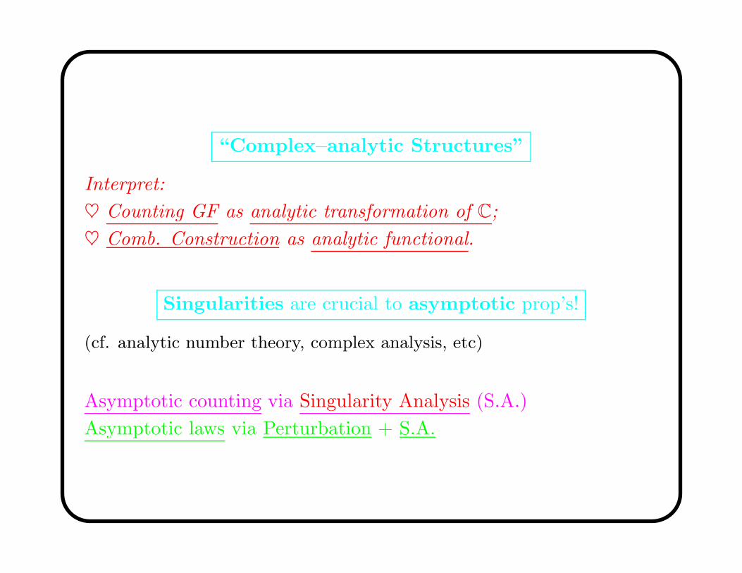
“Complex–analytic Structures”

Interpret:

♥ Counting GF as analytic transformation of C;

♥ Comb. Construction as analytic functional.

Singularities are crucial to asymptotic prop’s!

(cf. analytic number theory, complex analysis, etc)

Asymptotic counting via Singularity Analysis (S.A.)

Asymptotic laws via Perturbation + S.A.

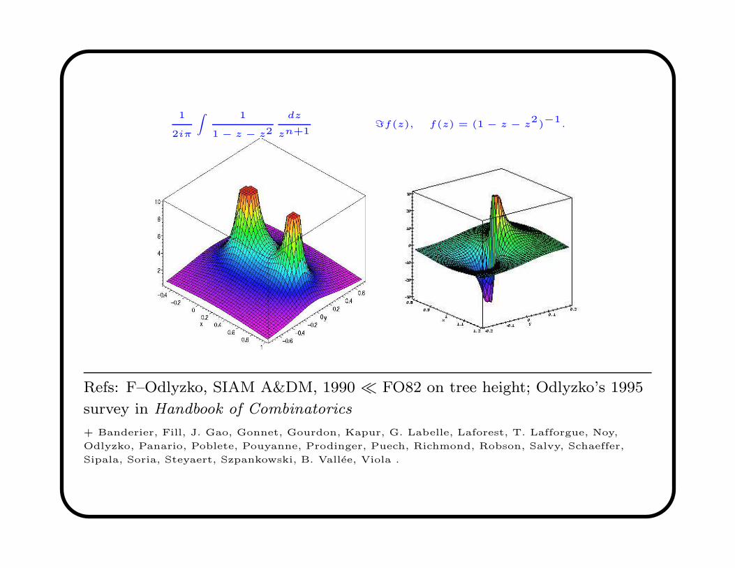
1

2iπ

Z 1

1 − z − z2

dz

zn+1=f(z), f(z) = (1 − z − z2)−1.

Refs: F–Odlyzko, SIAM A&DM, 1990 FO82 on tree height; Odlyzko’s 1995

survey in Handbook of Combinatorics

+ Banderier, Fill, J. Gao, Gonnet, Gourdon, Kapur, G. Labelle, Laforest, T. Lafforgue, Noy,

Odlyzko, Panario, Poblete, Pouyanne, Prodinger, Puech, Richmond, Robson, Salvy, Schaeffer,

Sipala, Soria, Steyaert, Szpankowski, B. Vallee, Viola .

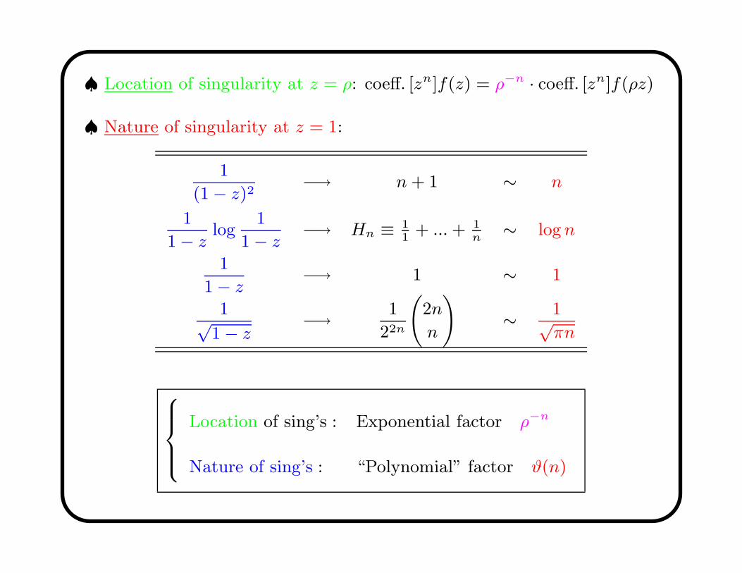
♠ Location of singularity at z = ρ: coeff. [zn]f(z) = ρ−n · coeff. [zn]f(ρz)

♠ Nature of singularity at z = 1:

1

(1 − z)2−→ n + 1 ∼ n

1

1 − zlog

1

1 − z−→ Hn ≡ 1

1+ ... + 1

n∼ log n

1

1 − z−→ 1 ∼ 1

1√1 − z

−→ 1

22n

2n

n

!∼ 1√

πn

8>><>>:

Location of sing’s : Exponential factor ρ−n

Nature of sing’s : “Polynomial” factor ϑ(n)

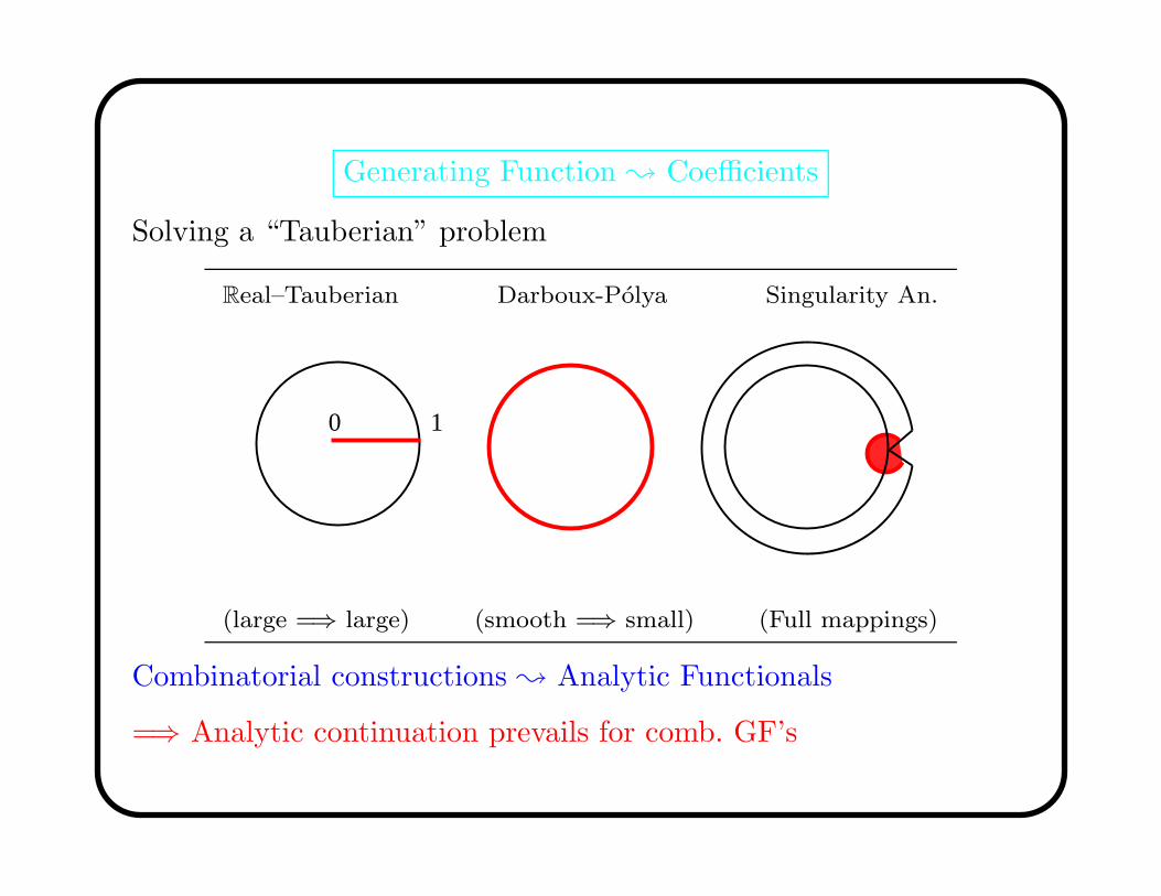
Generating Function ; Coefficients

Solving a “Tauberian” problem

Real–Tauberian Darboux-Polya Singularity An.

0 1

(large =⇒ large) (smooth =⇒ small) (Full mappings)

Combinatorial constructions ; Analytic Functionals

=⇒ Analytic continuation prevails for comb. GF’s

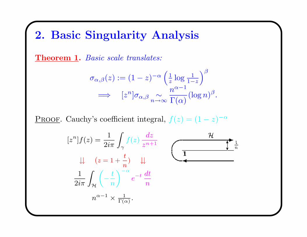
2. Basic Singularity Analysis

Theorem 1. Basic scale translates:

σα,β(z) := (1 − z)−α(

1

z log 1

1−z

)β

=⇒ [zn]σα,β ∼n→∞

nα−1

Γ(α)(log n)β .

Proof. Cauchy’s coefficient integral, f(z) = (1 − z)−α

[zn]f(z) =1

2iπ

Z

γ

f(z)dz

zn+1

↓↓ (z = 1 +t

n) ↓↓

1

2iπ

Z

H

„− t

n

«−α

e−t dt

n

nα−1 × 1Γ(α)

.

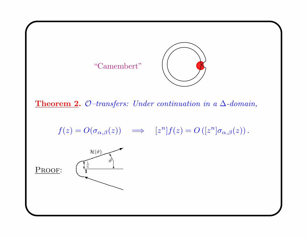
“Camembert”

Theorem 2. O–transfers: Under continuation in a ∆-domain,

f(z) = O(σα,β(z)) =⇒ [zn]f(z) = O ([zn]σα,β(z)) .

Proof:

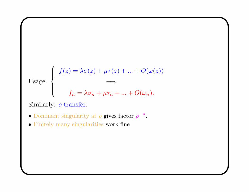
Usage:

f(z) = λσ(z) + µτ(z) + ... + O(ω(z))

=⇒fn = λσn + µτn + ... + O(ωn).

Similarly: o-transfer.

• Dominant singularity at ρ gives factor ρ−n.

• Finitely many singularities work fine

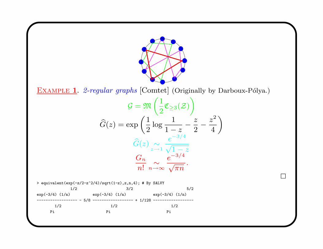
Example 1. 2-regular graphs [Comtet] (Originally by Darboux-Polya.)

G = M

„1

2C≥3(Z)

«

bG(z) = exp

„1

2log

1

1 − z− z

2− z2

4

«

bG(z) ∼z→1

e−3/4

√1 − z

Gn

n!∼

n→∞

e−3/4

√πn

.

2> equivalent(exp(-z/2-z^2/4)/sqrt(1-z),z,n,4); # By SALVY

1/2 3/2 5/2

exp(-3/4) (1/n) exp(-3/4) (1/n) exp(-3/4) (1/n)

------------------ - 5/8 ------------------ + 1/128 ------------------

1/2 1/2 1/2

Pi Pi Pi

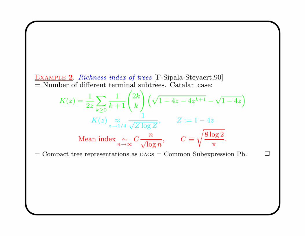
Example 2. Richness index of trees [F-Sipala-Steyaert,90]= Number of different terminal subtrees. Catalan case:

K(z) =1

2z

X

k≥0

1

k + 1

2k

k

!“p1 − 4z − 4zk+1 −

√1 − 4z

”

K(z) ≈z→1/4

1√Z log Z

, Z := 1 − 4z

Mean index ∼n→∞

Cn√log n

, C ≡r

8 log 2

π.

= Compact tree representations as dags = Common Subexpression Pb. 2

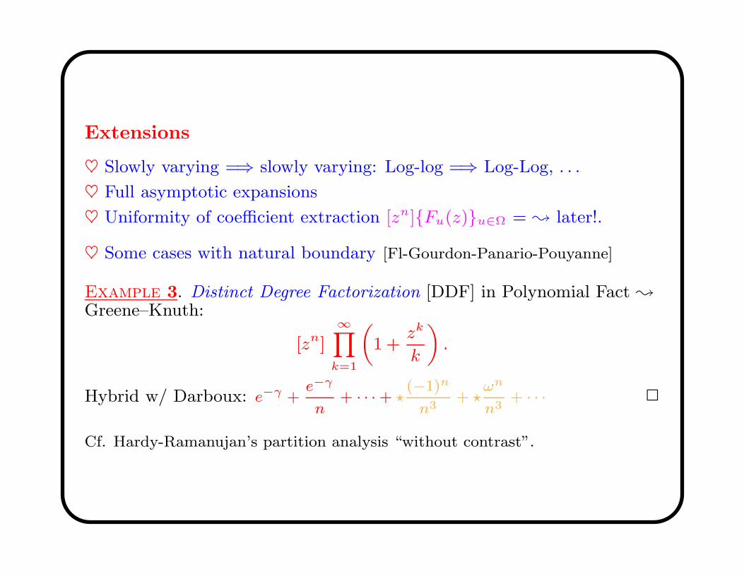
Extensions

♥ Slowly varying =⇒ slowly varying: Log-log =⇒ Log-Log, . . .

♥ Full asymptotic expansions

♥ Uniformity of coefficient extraction [zn]Fu(z)u∈Ω = ; later!.

♥ Some cases with natural boundary [Fl-Gourdon-Panario-Pouyanne]

Example 3. Distinct Degree Factorization [DDF] in Polynomial Fact ;

Greene–Knuth:

[zn]

∞Y

k=1

„1 +

zk

k

«.

Hybrid w/ Darboux: e−γ +e−γ

n+ · · · + ?

(−1)n

n3+ ?

ωn

n3+ · · · 2

Cf. Hardy-Ramanujan’s partition analysis “without contrast”.

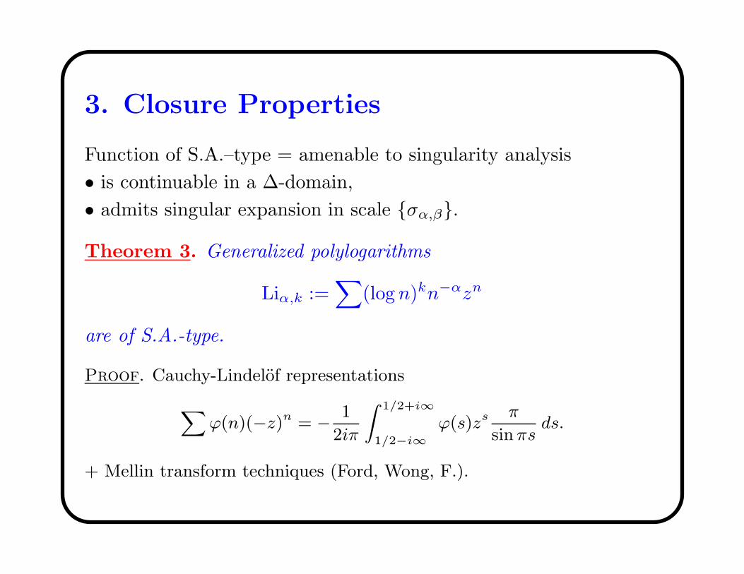
3. Closure Properties

Function of S.A.–type = amenable to singularity analysis

• is continuable in a ∆-domain,

• admits singular expansion in scale σα,β.

Theorem 3. Generalized polylogarithms

Liα,k :=∑

(log n)kn−αzn

are of S.A.-type.

Proof. Cauchy-Lindelof representations

Xϕ(n)(−z)n = − 1

2iπ

Z 1/2+i∞

1/2−i∞ϕ(s)zs π

sin πsds.

+ Mellin transform techniques (Ford, Wong, F.).

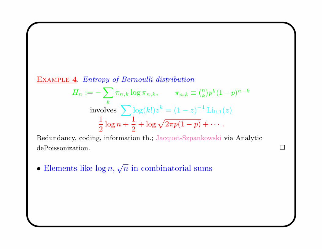
Example 4. Entropy of Bernoulli distribution

Hn := −X

k

πn,k log πn,k, πn,k ≡`n

k

´

pk(1 − p)n−k

involvesX

log(k!)zk = (1 − z)−1 Li0,1(z)1

2log n +

1

2+ log

p2πp(1 − p) + · · · .

Redundancy, coding, information th.; Jacquet-Szpankowski via Analytic

dePoissonization. 2

• Elements like log n,√

n in combinatorial sums

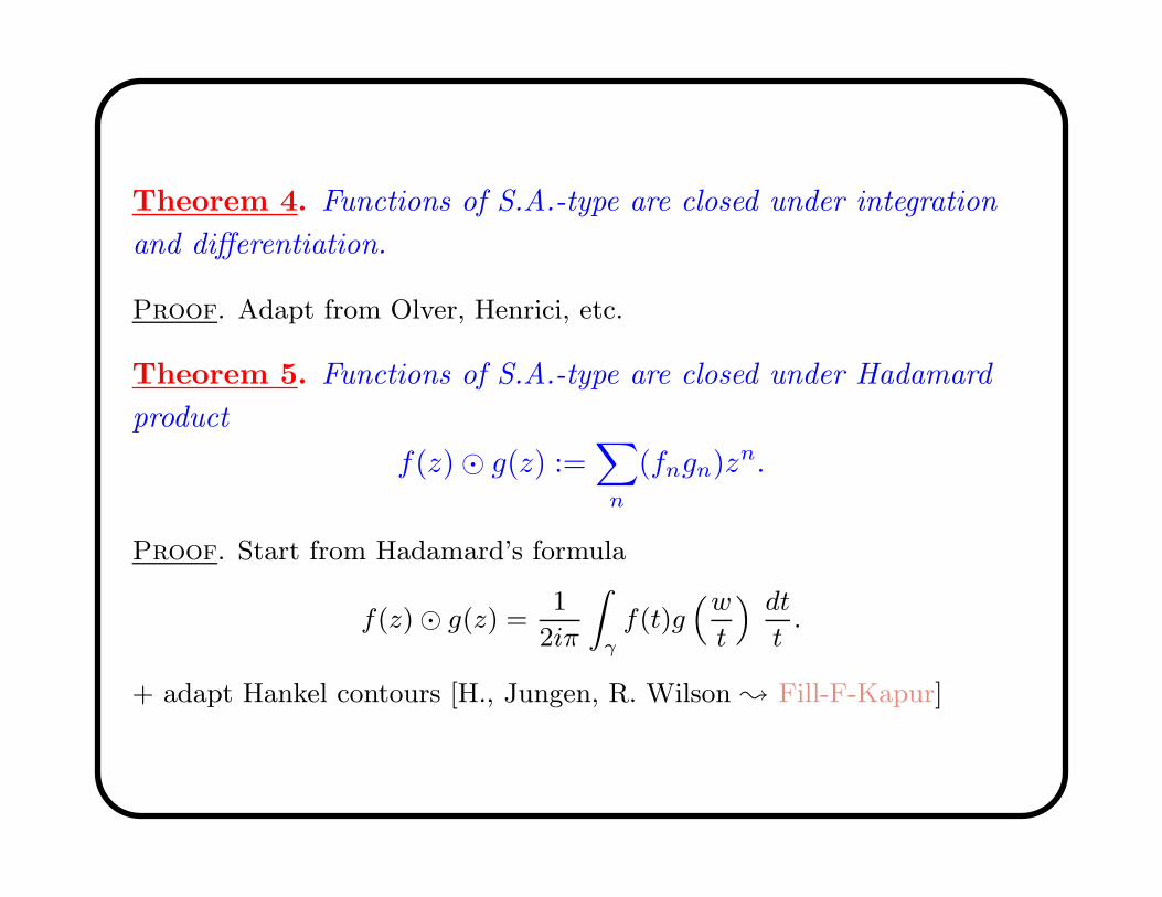
Theorem 4. Functions of S.A.-type are closed under integration

and differentiation.

Proof. Adapt from Olver, Henrici, etc.

Theorem 5. Functions of S.A.-type are closed under Hadamard

product

f(z) g(z) :=∑

n

(fngn)zn.

Proof. Start from Hadamard’s formula

f(z) g(z) =1

2iπ

Z

γ

f(t)g“w

t

” dt

t.

+ adapt Hankel contours [H., Jungen, R. Wilson ; Fill-F-Kapur]

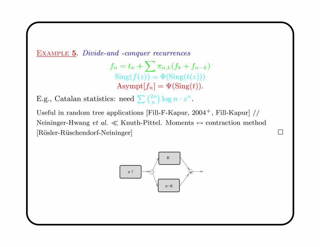
Example 5. Divide-and -conquer recurrences

fn = tn +X

πn,k(fk + fn−k)

Sing(f(z)) = Φ(Sing(t(z)))Asympt[fn] = Ψ(Sing(t)).

E.g., Catalan statistics: needP`

2nn

´log n · zn.

Useful in random tree applications [Fill-F-Kapur, 2004+, Fill-Kapur] //

Neininger-Hwang et al. Knuth-Pittel. Moments ↔ contraction method

[Rosler-Ruschendorf-Neininger] 2

n ?

K

n−K

*

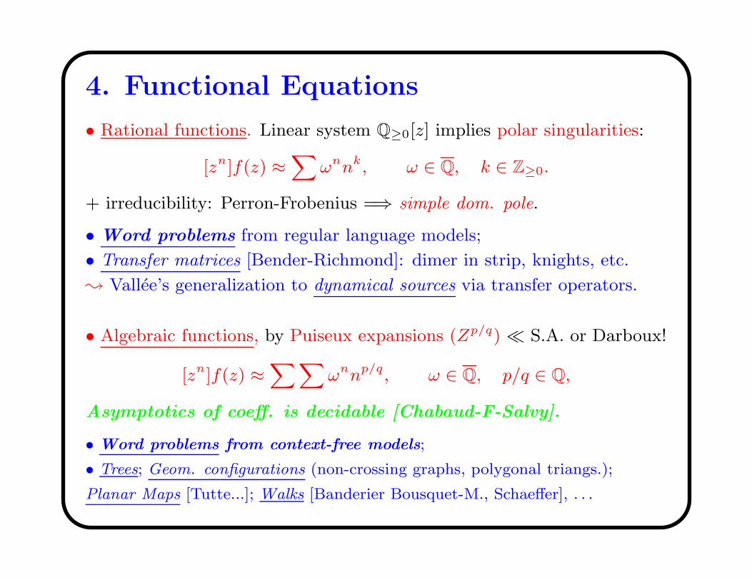
4. Functional Equations

• Rational functions. Linear system Q≥0[z] implies polar singularities:

[zn]f(z) ≈X

ωnnk, ω ∈ Q, k ∈ Z≥0.

+ irreducibility: Perron-Frobenius =⇒ simple dom. pole.

• Word problems from regular language models;

• Transfer matrices [Bender-Richmond]: dimer in strip, knights, etc.

; Vallee’s generalization to dynamical sources via transfer operators.

• Algebraic functions, by Puiseux expansions (Zp/q) S.A. or Darboux!

[zn]f(z) ≈XX

ωnnp/q, ω ∈ Q, p/q ∈ Q,

Asymptotics of coeff. is decidable [Chabaud-F-Salvy].

• Word problems from context-free models;

• Trees; Geom. configurations (non-crossing graphs, polygonal triangs.);

Planar Maps [Tutte...]; Walks [Banderier Bousquet-M., Schaeffer], . . .

(1 −√

1 − 4z)/(2z)

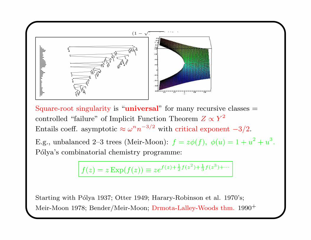
Square-root singularity is “universal” for many recursive classes =

controlled “failure” of Implicit Function Theorem Z ∝ Y 2

Entails coeff. asymptotic ≈ ωnn−3/2 with critical exponent −3/2.

E.g., unbalanced 2–3 trees (Meir-Moon): f = zφ(f), φ(u) = 1 + u2 + u3.

Polya’s combinatorial chemistry programme:

f(z) = z Exp(f(z)) ≡ zef(z)+ 12

f(z2)+ 13

f(z3)+···

Starting with Polya 1937; Otter 1949; Harary-Robinson et al. 1970’s;

Meir-Moon 1978; Bender/Meir-Moon; Drmota-Lalley-Woods thm. 1990+

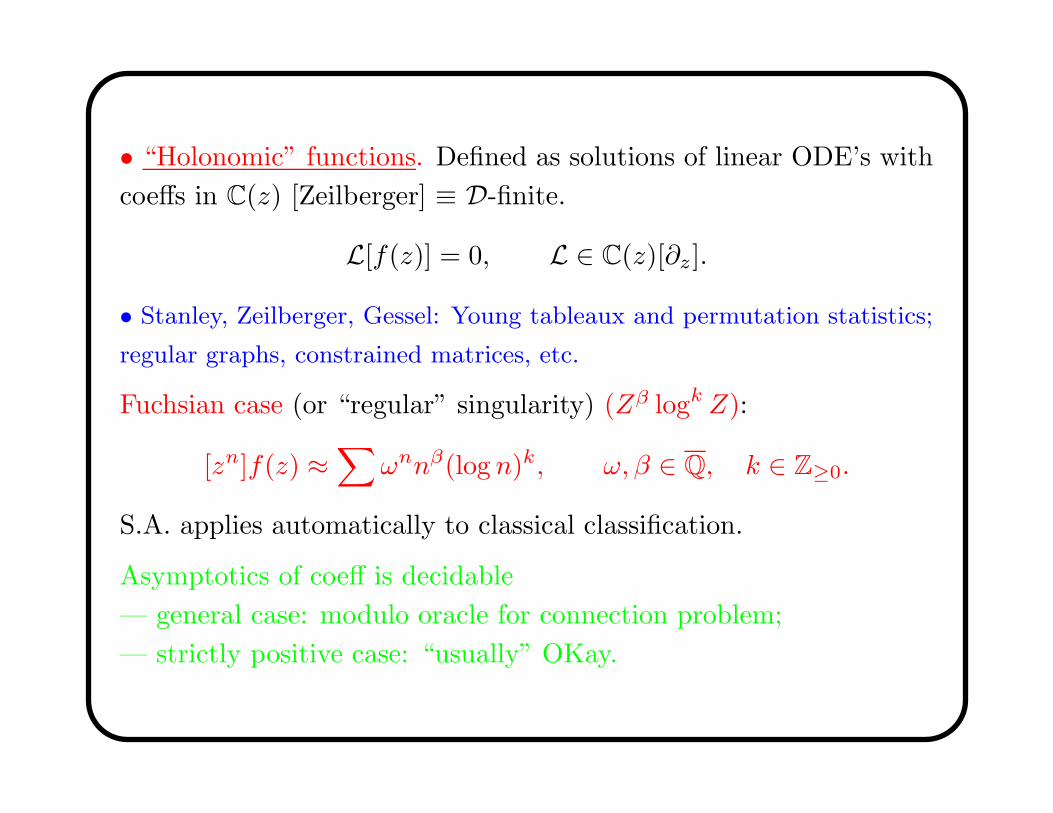
• “Holonomic” functions. Defined as solutions of linear ODE’s with

coeffs in C(z) [Zeilberger] ≡ D-finite.

L[f(z)] = 0, L ∈ C(z)[∂z].

• Stanley, Zeilberger, Gessel: Young tableaux and permutation statistics;

regular graphs, constrained matrices, etc.

Fuchsian case (or “regular” singularity) (Zβ logk Z):

[zn]f(z) ≈∑

ωnnβ(log n)k, ω, β ∈ Q, k ∈ Z≥0.

S.A. applies automatically to classical classification.

Asymptotics of coeff is decidable

— general case: modulo oracle for connection problem;

— strictly positive case: “usually” OKay.

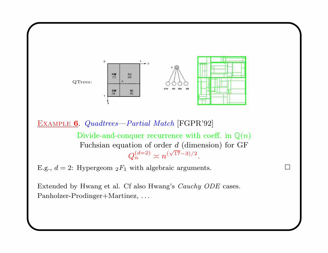
QTrees:

Example 6. Quadtrees—Partial Match [FGPR’92]

Divide-and-conquer recurrence with coeff. in Q(n)Fuchsian equation of order d (dimension) for GF

Q(d=2)n n(

√17−3)/2.

E.g., d = 2: Hypergeom 2F1 with algebraic arguments. 2

Extended by Hwang et al. Cf also Hwang’s Cauchy ODE cases.

Panholzer-Prodinger+Martinez, . . .

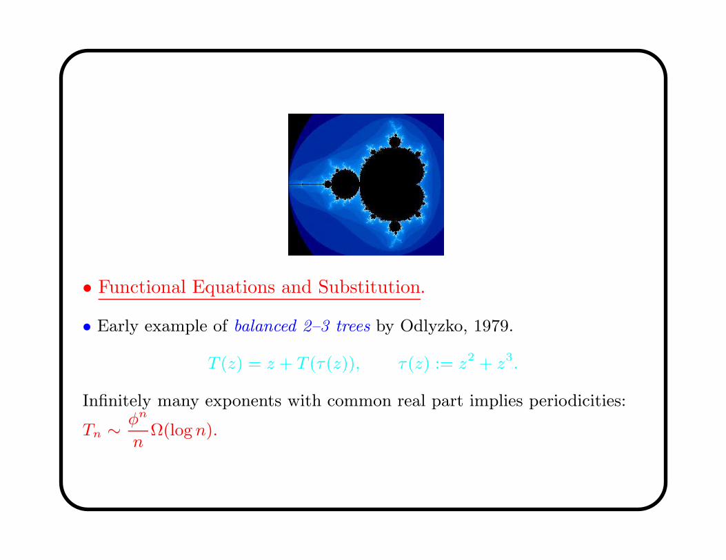
• Functional Equations and Substitution.

• Early example of balanced 2–3 trees by Odlyzko, 1979.

T (z) = z + T (τ(z)), τ(z) := z2 + z3.

Infinitely many exponents with common real part implies periodicities:

Tn ∼ φn

nΩ(log n).

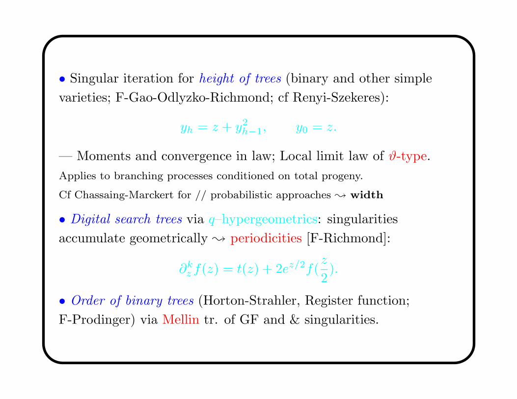
• Singular iteration for height of trees (binary and other simple

varieties; F-Gao-Odlyzko-Richmond; cf Renyi-Szekeres):

yh = z + y2

h−1, y0 = z.

— Moments and convergence in law; Local limit law of ϑ-type.

Applies to branching processes conditioned on total progeny.

Cf Chassaing-Marckert for // probabilistic approaches ; width

• Digital search trees via q–hypergeometrics: singularities

accumulate geometrically ; periodicities [F-Richmond]:

∂kz f(z) = t(z) + 2ez/2f(

z

2).

• Order of binary trees (Horton-Strahler, Register function;

F-Prodinger) via Mellin tr. of GF and & singularities.

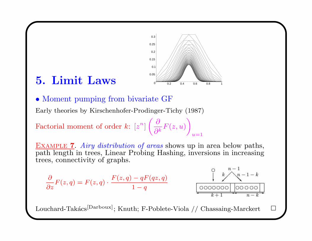
5. Limit Laws 0

0.05

0.1

0.15

0.2

0.25

0.3

0.2 0.4 0.6 0.8 1

• Moment pumping from bivariate GF

Early theories by Kirschenhofer-Prodinger-Tichy (1987)

Factorial moment of order k: [zn]

„∂

∂kF (z, u)

«

u=1

Example 7. Airy distribution of areas shows up in area below paths,path length in trees, Linear Probing Hashing, inversions in increasingtrees, connectivity of graphs.

∂

∂zF (z, q) = F (z, q) ·

F (z, q) − qF (qz, q)

1 − q

Louchard-Takacs[Darboux]; Knuth; F-Poblete-Viola // Chassaing-Marckert 2

Classical probability theory: sums of Random Variables ; powers

of fixed function (PGF, Fourier tr.) ; Normal Law.

For problems expressed by Bivariate GF (BGF): field founded by E.

Bender et al. + developments by F, Soria, Hwang, . . .

Idea: BGF F (z, u) =X

fn(u)zn, where fn(u) describes parameter on

objects of size n. If (for u near 1)

fn(u) ≈ ω(u)κn , κn → ∞,

then speak of Quasi-Powers approximation. Recycle continuity

theorem, Berry-Esseen, Chernov, etc. =⇒ Normal law and many

goodies. . .

(speed of convergence, large deviation fn, local limits)

Two important cases:

• Movable singularity:

F (z, u) ≈„

1 − z

ρ(u)

«−α

=⇒ fn(u)

fn(1)≈„

ρ(1)

ρ(u)

«n

.

• Variable exponent:

F (z, u) ≈„

1 − z

ρ

«−α(u)

=⇒ fn(u)

fn(1)≈

8<:

nα(u)−α(1)

“eα(u)−α(1)

”log n

.

Requires uniformity afforded by Singularity Analysis

(6= Tauber or Darboux).

Singularity Perturbation analysis (smoothness)

↓Uniform Quasi-Powers for coeffs

↓Normal limit law

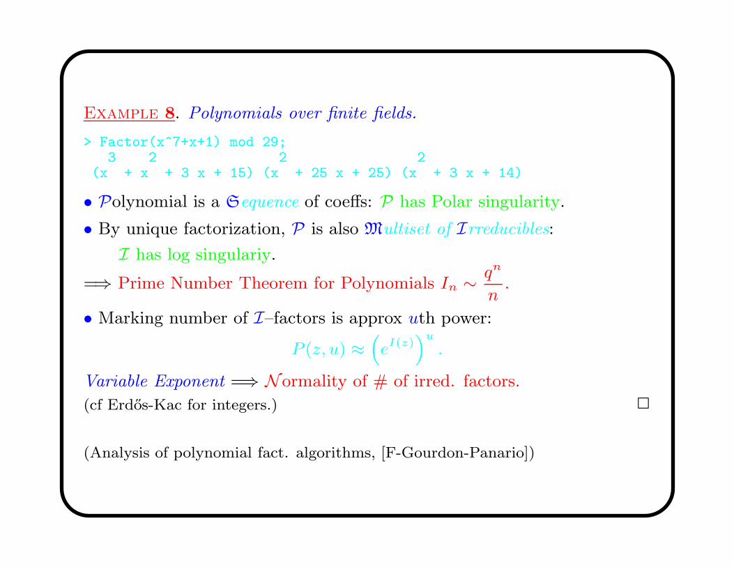
Example 8. Polynomials over finite fields.

> Factor(x^7+x+1) mod 29;3 2 2 2

(x + x + 3 x + 15) (x + 25 x + 25) (x + 3 x + 14)

• Polynomial is a Sequence of coeffs: P has Polar singularity.

• By unique factorization, P is also Multiset of Irreducibles:

I has log singulariy.

=⇒ Prime Number Theorem for Polynomials In ∼ qn

n.

• Marking number of I–factors is approx uth power:

P (z, u) ≈“eI(z)

”u

.

Variable Exponent =⇒ Normality of # of irred. factors.

(cf Erdos-Kac for integers.) 2

(Analysis of polynomial fact. algorithms, [F-Gourdon-Panario])

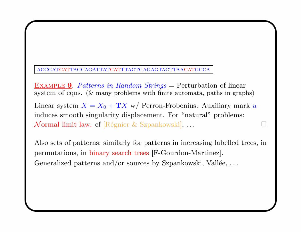
accgatcattagcagattatcatttactgagagtacttaacatgcca

Example 9. Patterns in Random Strings = Perturbation of linearsystem of eqns. (& many problems with finite automata, paths in graphs)

Linear system X = X0 + TX w/ Perron-Frobenius. Auxiliary mark u

induces smooth singularity displacement. For “natural” problems:

Normal limit law. cf [Regnier & Szpankowski], . . . 2

Also sets of patterns; similarly for patterns in increasing labelled trees, in

permutations, in binary search trees [F-Gourdon-Martinez].

Generalized patterns and/or sources by Szpankowski, Vallee, . . .

-0.5

-0.4

-0.3

-0.2

-0.1

0

0.1

-0.15 -0.1 -0.05 0.05 0.1

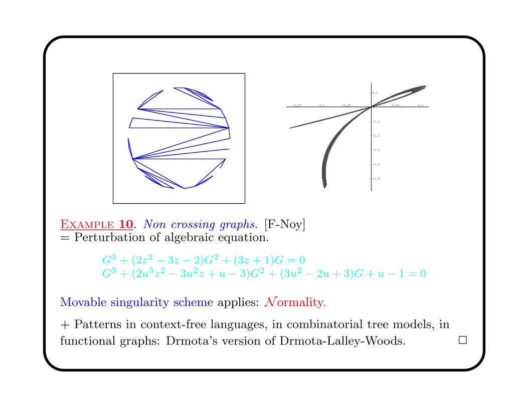
Example 10. Non crossing graphs. [F-Noy]= Perturbation of algebraic equation.

G3 + (2z2 − 3z − 2)G2 + (3z + 1)G = 0G3 + (2u3z2 − 3u2z + u − 3)G2 + (3u2 − 2u + 3)G + u − 1 = 0

Movable singularity scheme applies: Normality.

+ Patterns in context-free languages, in combinatorial tree models, in

functional graphs: Drmota’s version of Drmota-Lalley-Woods. 2

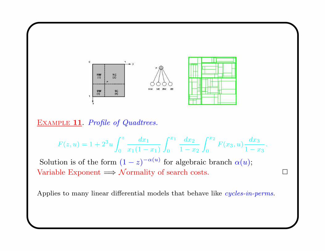
Example 11. Profile of Quadtrees.

F (z, u) = 1 + 23u

Z z

0

dx1

x1(1 − x1)

Z x1

0

dx2

1 − x2

Z x2

0F (x3, u)

dx3

1 − x3.

Solution is of the form (1 − z)−α(u) for algebraic branch α(u);

Variable Exponent =⇒ Normality of search costs. 2

Applies to many linear differential models that behave like cycles-in-perms.

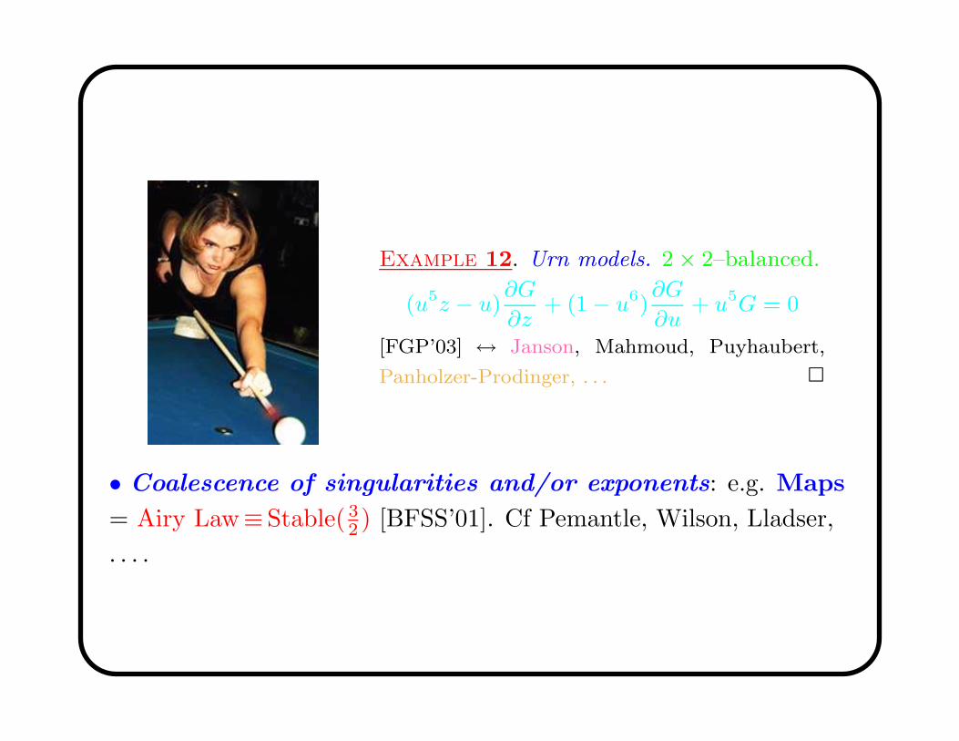
Example 12. Urn models. 2 × 2–balanced.

(u5z − u)∂G

∂z+ (1 − u6)

∂G

∂u+ u5G = 0

[FGP’03] ↔ Janson, Mahmoud, Puyhaubert,

Panholzer-Prodinger, . . . 2

• Coalescence of singularities and/or exponents: e.g. Maps

= Airy Law≡ Stable( 3

2) [BFSS’01]. Cf Pemantle, Wilson, Lladser,

. . . .

Conclusions

For combinatorial counting and limit laws:

Modest technical apparatus & generic technology.

High-level for applications, esp., analysis of algorithms.

Plug-in on Symbolic Combinatorics & Symbolic Computation.

Discussion of Schemas & “Universality” in metric aspects of

random discrete structures.

E.g. Borges’ theorem for words, trees, labelled trees, mappings, permutations,

increasing trees, maps, etc.

Thank you!

♥♥♥