5th High Performance Yacht Design Conference Auckland, 10-12 March, 2015

Singularity MAXI: A comparison of CFD and Tank test results

Oleg Gulinsky, bedelbaeva_aigul@mail.ru Andrey Rogatkin, andreyrogatkin@gmail.com

Vadim Vorobyov, mrvorobus@gmail.com

Abstract. The boat concept of Lutra 80 Singularity was to create a true dual-purpose yacht that rewards its owner with racecourse performance and a high level of interior luxury. The hull form and underwater appendages combined with an aggressive sail plan showed impressive results on the racecourse. This task has required a significant amount of tank and tunnel tests. Not all the planned tests could be carried out within a limited time and with a certain constraint on the budget. This report presents the results of a series of CFD experiments based on the OpenFOAM platform. Marin tank test gave results which were confirmed in the real tests in the sea. The main purpose of our computations at this stage is to reproduce the resistance (drag) curves at various heeling angles. We used different mesh sizes and configurations. In general, we achieved a good correspondence (within 10%) between CFD and Marin tank test results. However this correspondence is not uniform. For more accurate results, it is necessary to apply refinement of the mesh, and continue to search for suitable regularization parameters.

NOMENCLATURE w Wall shear stress α Relative amount of water in computational cell ρ Weighted media density ρw Water density ρa Air density µ Weighted dynamic viscosity µt Turbulence dynamic viscosity ν w Water kinematic viscosity ν a Air kinematic viscosity ν Weighted kinematic viscosity U Velocity vector field P Pressure field y+ Dimensionless wall distance u+ Dimensionless velocity κ Von Karman constant FB Body forces

1. INTRODUCTION

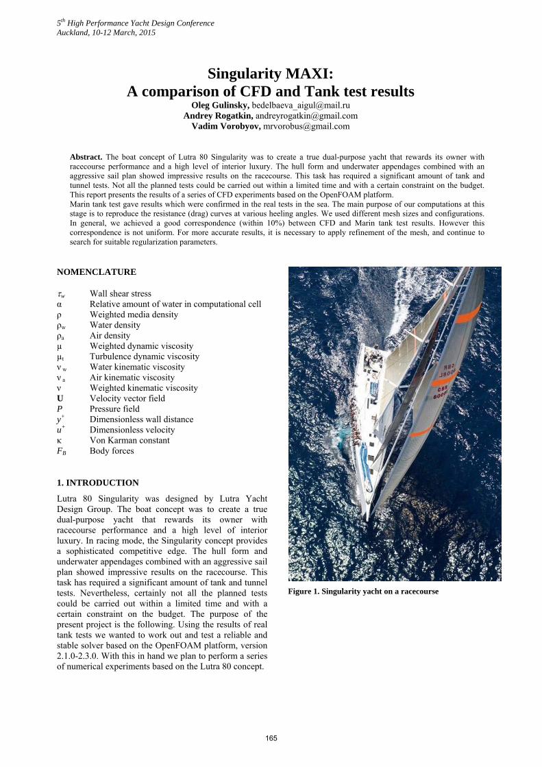
Lutra 80 Singularity was designed by Lutra Yacht Design Group. The boat concept was to create a true dual-purpose yacht that rewards its owner with racecourse performance and a high level of interior luxury. In racing mode, the Singularity concept provides a sophisticated competitive edge. The hull form and underwater appendages combined with an aggressive sail plan showed impressive results on the racecourse. This task has required a significant amount of tank and tunnel tests. Nevertheless, certainly not all the planned tests could be carried out within a limited time and with a certain constraint on the budget. The purpose of the present project is the following. Using the results of real tank tests we wanted to work out and test a reliable and stable solver based on the OpenFOAM platform, version 2.1.0-2.3.0. With this in hand we plan to perform a series of numerical experiments based on the Lutra 80 concept.

Figure 1. Singularity yacht on a racecourse

165

2. COMPUTATIONAL PROCEDURE

2.1. Navier-Stokes numerical solving

The starting point is the Navier-Stokes equation, which is now believed to embody the physics of all fluid flows, including turbulent ones (in the simple form appropriate for analysis of incompressible flow of a fluid whose physical properties may be assumed constant):

· 0, U ∙ ∙

There are several approaches to the construction of approximate solutions of the equations such as RANS, LES and DNS. For detailed discussion LES, DNS and RANS see for example [1]. On this stage of study we basically used RANS. For more information on CFD theory see [2].

2.2. Two phase fluid

A yacht hull design problem is commonly referred to a hydrodynamic one. However, this can lead to confusion, because in fact it is substantially a two-phase flow problem. Indeed, the wave drag force is essential for conventional ships and not for submarines in deep water. Consequently, we need to simulate a boat moving in a two-phase medium and, what is most important, an interaction between the air and water phases. On the other hand, the forces acting on hull are not equally affected by these two phases. As the density of air is much less than the density of water, it makes no sense to model an exact air velocity field and a pressure distribution. However, what we do need to determine is the air-water interface precise position and the air-water mixing proportions in a region where such mixing exists. We use VOF method which consider two immiscible fluids as one effective fluid in the domain, the physical properties of which are calculated as weighted averages:

(1 )w a  ,

(1 )w w a a  ,

 , 

∙ 0 , ∙ ∙

2.3. Equation discretization

At this stage, our goal was to construct a reliable and stable computational scheme, so in some cases we chose the lower order schemes which at the same time provide a bounded solution. To that end, we have chosen the finite volume method (FV). In this method physical properties of the flow for each cell assumed constant in this cell and are attributed to the cell geometric center. For interpolation of the divergent term in the turbulence model equation we applied the Upwind Differencing (UD) discretization scheme. Boundedness of the UD solution is guaranteed through the sufficient boundedness criterion for systems of algebraic equations. However, boundedness of UD is insured at the expense of the accuracy.

2.4. Dynamic Mesh handling

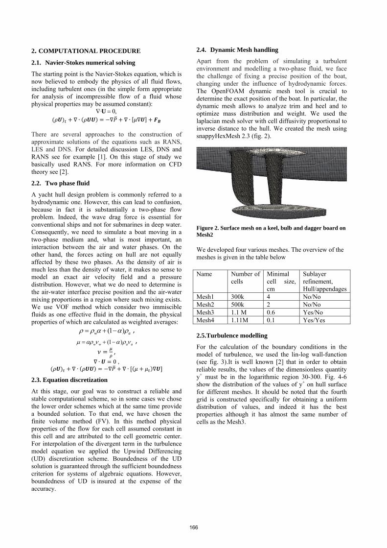
Apart from the problem of simulating a turbulent environment and modelling a two-phase fluid, we face the challenge of fixing a precise position of the boat, changing under the influence of hydrodynamic forces. The OpenFOAM dynamic mesh tool is crucial to determine the exact position of the boat. In particular, the dynamic mesh allows to analyze trim and heel and to optimize mass distribution and weight. We used the laplacian mesh solver with cell diffusivity proportional to inverse distance to the hull. We created the mesh using snappyHexMesh 2.3 (fig. 2).

Figure 2. Surface mesh on a keel, bulb and dagger board on Mesh2

We developed four various meshes. The overview of the meshes is given in the table below Name Number of

cells Minimal cell size, cm

Sublayer refinement, Hull/appendages

Mesh1 300k 4 No/No Mesh2 500k 2 No/No Mesh3 1.1 M 0.6 Yes/No Mesh4 1.11M 0.1 Yes/Yes 2.5.Turbulence modelling

For the calculation of the boundary conditions in the model of turbulence, we used the lin-log wall-function (see fig. 3).It is well known [2] that in order to obtain reliable results, the values of the dimensionless quantity y+ must be in the logarithmic region 30-300. Fig. 4-6 show the distribution of the values of y+ on hull surface for different meshes. It should be noted that the fourth grid is constructed specifically for obtaining a uniform distribution of values, and indeed it has the best properties although it has almost the same number of cells as the Mesh3.

166

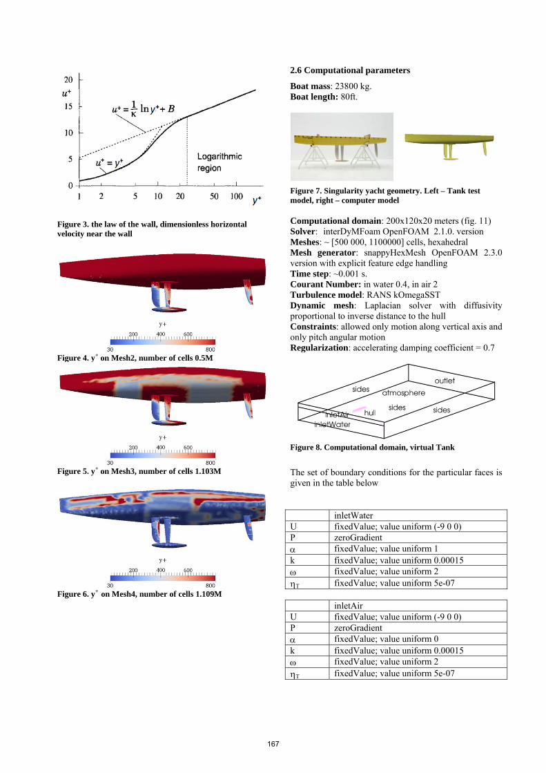
Figure 3. the law of the wall, dimensionless horizontal velocity near the wall

Figure 4. y+ on Mesh2, number of cells 0.5M

Figure 5. y+ on Mesh3, number of cells 1.103M

Figure 6. y+ on Mesh4, number of cells 1.109M

2.6 Computational parameters

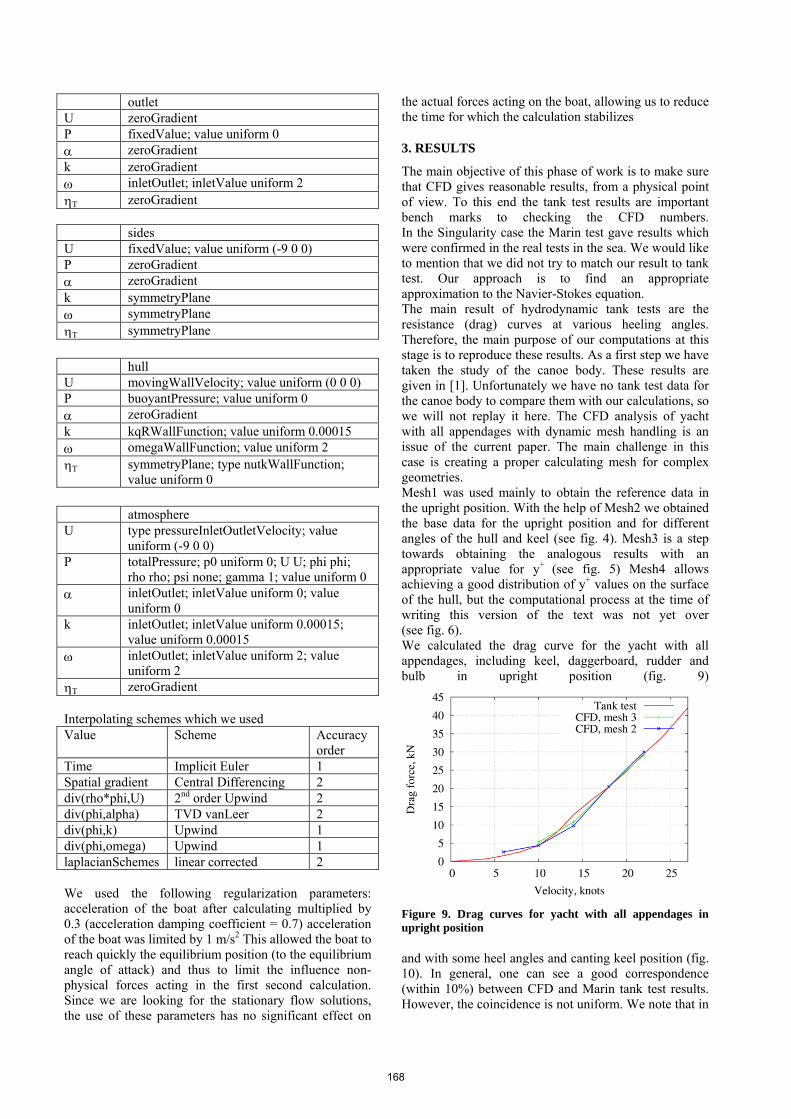
Boat mass: 23800 kg. Boat length: 80ft.

Figure 7. Singularity yacht geometry. Left – Tank test model, right – computer model Computational domain: 200x120x20 meters (fig. 11) Solver: interDyMFoam OpenFOAM 2.1.0. version Meshes: ~ [500 000, 1100000] cells, hexahedral Mesh generator: snappyHexMesh OpenFOAM 2.3.0 version with explicit feature edge handling Time step: ~0.001 s. Courant Number: in water 0.4, in air 2 Turbulence model: RANS kOmegaSST Dynamic mesh: Laplacian solver with diffusivity proportional to inverse distance to the hull Constraints: allowed only motion along vertical axis and only pitch angular motion Regularization: accelerating damping coefficient = 0.7

Figure 8. Computational domain, virtual Tank

The set of boundary conditions for the particular faces is given in the table below

inletWater U fixedValue; value uniform (-9 0 0) P zeroGradient fixedValue; value uniform 1 k fixedValue; value uniform 0.00015 fixedValue; value uniform 2 T fixedValue; value uniform 5e-07 inletAir U fixedValue; value uniform (-9 0 0) P zeroGradient fixedValue; value uniform 0 k fixedValue; value uniform 0.00015 fixedValue; value uniform 2 T fixedValue; value uniform 5e-07

167

outlet U zeroGradient P fixedValue; value uniform 0 zeroGradient k zeroGradient inletOutlet; inletValue uniform 2 T zeroGradient sides U fixedValue; value uniform (-9 0 0) P zeroGradient zeroGradient k symmetryPlane symmetryPlane T symmetryPlane

hull U movingWallVelocity; value uniform (0 0 0) P buoyantPressure; value uniform 0 zeroGradient k kqRWallFunction; value uniform 0.00015 omegaWallFunction; value uniform 2 T symmetryPlane; type nutkWallFunction;

value uniform 0

atmosphere U type pressureInletOutletVelocity; value

uniform (-9 0 0) P totalPressure; p0 uniform 0; U U; phi phi;

rho rho; psi none; gamma 1; value uniform 0 inletOutlet; inletValue uniform 0; value

uniform 0 k inletOutlet; inletValue uniform 0.00015;

value uniform 0.00015 inletOutlet; inletValue uniform 2; value

uniform 2 T zeroGradient Interpolating schemes which we used Value Scheme Accuracy

order Time Implicit Euler 1 Spatial gradient Central Differencing 2 div(rho*phi,U) 2nd order Upwind 2 div(phi,alpha) TVD vanLeer 2 div(phi,k) Upwind 1 div(phi,omega) Upwind 1 laplacianSchemes linear corrected 2 We used the following regularization parameters: acceleration of the boat after calculating multiplied by 0.3 (acceleration damping coefficient = 0.7) acceleration of the boat was limited by 1 m/s2 This allowed the boat to reach quickly the equilibrium position (to the equilibrium angle of attack) and thus to limit the influence non-physical forces acting in the first second calculation. Since we are looking for the stationary flow solutions, the use of these parameters has no significant effect on

the actual forces acting on the boat, allowing us to reduce the time for which the calculation stabilizes

3. RESULTS

The main objective of this phase of work is to make sure that CFD gives reasonable results, from a physical point of view. To this end the tank test results are important bench marks to checking the CFD numbers. In the Singularity case the Marin test gave results which were confirmed in the real tests in the sea. We would like to mention that we did not try to match our result to tank test. Our approach is to find an appropriate approximation to the Navier-Stokes equation. The main result of hydrodynamic tank tests are the resistance (drag) curves at various heeling angles. Therefore, the main purpose of our computations at this stage is to reproduce these results. As a first step we have taken the study of the canoe body. These results are given in [1]. Unfortunately we have no tank test data for the canoe body to compare them with our calculations, so we will not replay it here. The CFD analysis of yacht with all appendages with dynamic mesh handling is an issue of the current paper. The main challenge in this case is creating a proper calculating mesh for complex geometries. Mesh1 was used mainly to obtain the reference data in the upright position. With the help of Mesh2 we obtained the base data for the upright position and for different angles of the hull and keel (see fig. 4). Mesh3 is a step towards obtaining the analogous results with an appropriate value for y+ (see fig. 5) Mesh4 allows achieving a good distribution of y+ values on the surface of the hull, but the computational process at the time of writing this version of the text was not yet over (see fig. 6). We calculated the drag curve for the yacht with all appendages, including keel, daggerboard, rudder and bulb in upright position (fig. 9)

Figure 9. Drag curves for yacht with all appendages in upright position

and with some heel angles and canting keel position (fig. 10). In general, one can see a good correspondence (within 10%) between CFD and Marin tank test results. However, the coincidence is not uniform. We note that in

168

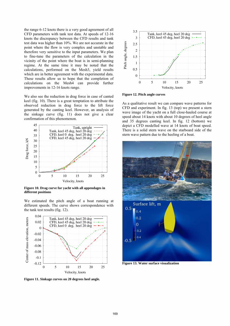
the range 6-12 knots there is a very good agreement of all CFD parameters with tank test data. At speeds of 12-16 knots the discrepancy between the CFD results and tank test data was higher than 10%. We are not accurate in the point where the flow is very complex and unstable and therefore very sensitive to the input parameters. We plan to fine-tune the parameters of the calculation in the vicinity of the point where the boat is in semi-planning regime. At the same time it may be noted that the calculations, performed on the Mesh3, yield results which are in better agreement with the experimental data. These results allow us to hope that the completion of calculations on the Mesh4 can provide further improvements in 12-16 knots range. We also see the reduction in drag force in case of canted keel (fig. 10). There is a great temptation to attribute the observed reduction in drag force to the lift force generated by the canting keel. However, an analysis of the sinkage curve (fig. 11) does not give a clear confirmation of this phenomenon.

Figure 10. Drag curve for yacht with all appendages in different positions

We estimated the pitch angle of a boat running at different speeds. The curve shows correspondence with the tank test results (fig. 12).

Figure 11. Sinkage curves on 20 degrees heel angle.

Figure 12. Pitch angle curves

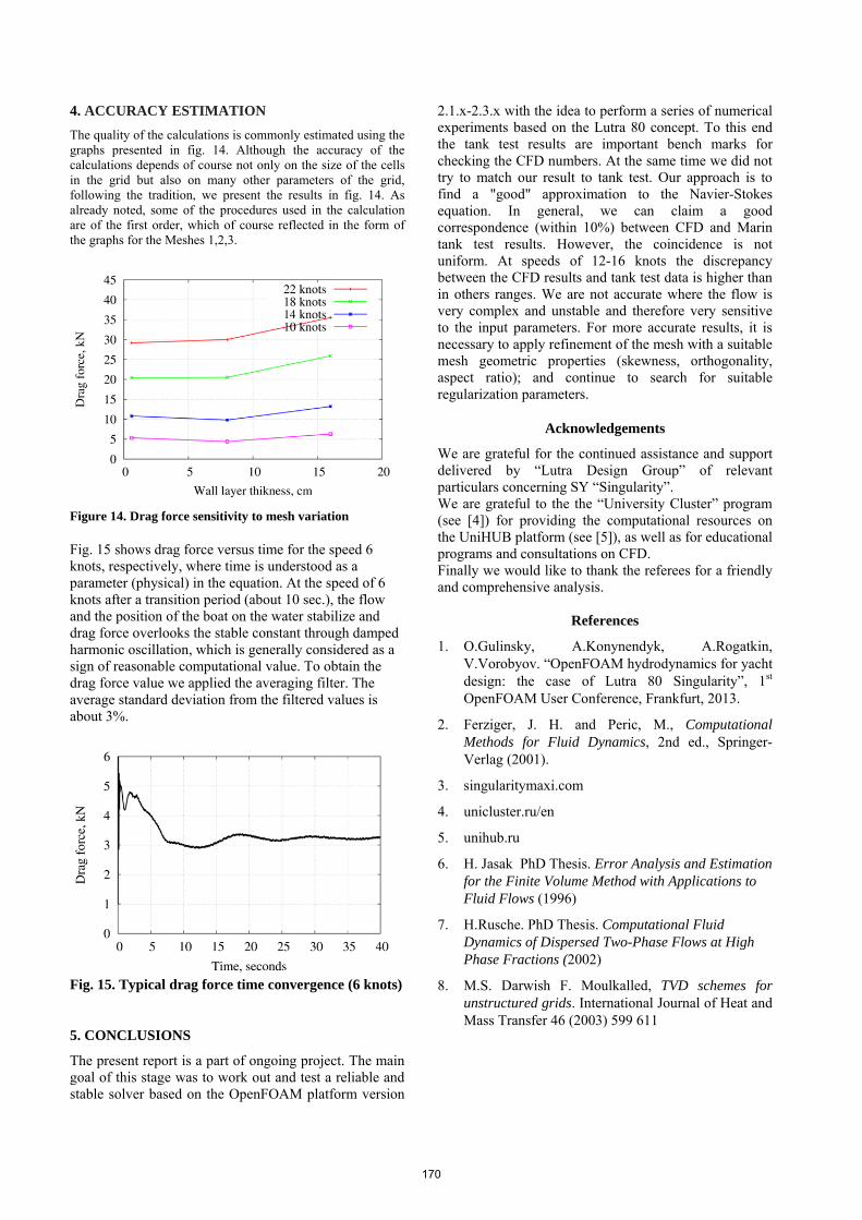
As a qualitative result we can compare wave patterns for CFD and experiment. In fig. 13 (top) we present a stern wave image of the yacht on a full close-hauled course at speed about 14 knots with about 10 degrees of heel angle and 35 degrees canting keel. In fig. 12 (bottom) we depict a CFD modelled wave at 14 knots of boat speed. There is a solid stern wave on the starboard side of the stern wave pattern due to the heeling of a boat.

Figure 13. Water surface visualization

169

4. ACCURACY ESTIMATION

The quality of the calculations is commonly estimated using the graphs presented in fig. 14. Although the accuracy of the calculations depends of course not only on the size of the cells in the grid but also on many other parameters of the grid, following the tradition, we present the results in fig. 14. As already noted, some of the procedures used in the calculation are of the first order, which of course reflected in the form of the graphs for the Meshes 1,2,3.

Figure 14. Drag force sensitivity to mesh variation

Fig. 15 shows drag force versus time for the speed 6 knots, respectively, where time is understood as a parameter (physical) in the equation. At the speed of 6 knots after a transition period (about 10 sec.), the flow and the position of the boat on the water stabilize and drag force overlooks the stable constant through damped harmonic oscillation, which is generally considered as a sign of reasonable computational value. To obtain the drag force value we applied the averaging filter. The average standard deviation from the filtered values is about 3%.

Fig. 15. Typical drag force time convergence (6 knots)

5. CONCLUSIONS

The present report is a part of ongoing project. The main goal of this stage was to work out and test a reliable and stable solver based on the OpenFOAM platform version

2.1.x-2.3.x with the idea to perform a series of numerical experiments based on the Lutra 80 concept. To this end the tank test results are important bench marks for checking the CFD numbers. At the same time we did not try to match our result to tank test. Our approach is to find a "good" approximation to the Navier-Stokes equation. In general, we can claim a good correspondence (within 10%) between CFD and Marin tank test results. However, the coincidence is not uniform. At speeds of 12-16 knots the discrepancy between the CFD results and tank test data is higher than in others ranges. We are not accurate where the flow is very complex and unstable and therefore very sensitive to the input parameters. For more accurate results, it is necessary to apply refinement of the mesh with a suitable mesh geometric properties (skewness, orthogonality, aspect ratio); and continue to search for suitable regularization parameters.

Acknowledgements

We are grateful for the continued assistance and support delivered by “Lutra Design Group” of relevant particulars concerning SY “Singularity”. We are grateful to the the “University Cluster” program (see [4]) for providing the computational resources on the UniHUB platform (see [5]), as well as for educational programs and consultations on CFD. Finally we would like to thank the referees for a friendly and comprehensive analysis.

References

1. O.Gulinsky, A.Konynendyk, A.Rogatkin, V.Vorobyov. “OpenFOAM hydrodynamics for yacht design: the case of Lutra 80 Singularity”, 1st OpenFOAM User Conference, Frankfurt, 2013.

2. Ferziger, J. H. and Peric, M., Computational Methods for Fluid Dynamics, 2nd ed., Springer-Verlag (2001).

3. singularitymaxi.com

4. unicluster.ru/en

5. unihub.ru

6. H. Jasak PhD Thesis. Error Analysis and Estimation for the Finite Volume Method with Applications to Fluid Flows (1996)

7. H.Rusche. PhD Thesis. Computational Fluid Dynamics of Dispersed Two-Phase Flows at High Phase Fractions (2002)

8. M.S. Darwish F. Moulkalled, TVD schemes for unstructured grids. International Journal of Heat and Mass Transfer 46 (2003) 599 611

170