Embed Size (px)
Citation preview
121
Sinusoidal regression
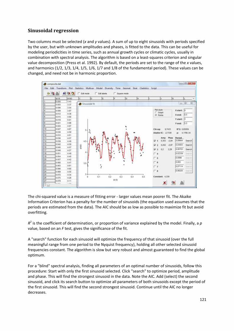
Two columns must be selected (x and y values). A sum of up to eight sinusoids with periods specified by the user, but with unknown amplitudes and phases, is fitted to the data. This can be useful for modeling periodicities in time series, such as annual growth cycles or climatic cycles, usually in combination with spectral analysis. The algorithm is based on a least-squares criterion and singular value decomposition (Press et al. 1992). By default, the periods are set to the range of the x values, and harmonics (1/2, 1/3, 1/4, 1/5, 1/6, 1/7 and 1/8 of the fundamental period). These values can be changed, and need not be in harmonic proportion.
The chi-squared value is a measure of fitting error - larger values mean poorer fit. The Akaike Information Criterion has a penalty for the number of sinusoids (the equation used assumes that the periods are estimated from the data). The AIC should be as low as possible to maximize fit but avoid overfitting.
R2 is the coefficient of determination, or proportion of variance explained by the model. Finally, a p value, based on an F test, gives the significance of the fit.
A "search" function for each sinusoid will optimize the frequency of that sinusoid (over the full meaningful range from one period to the Nyquist frequency), holding all other selected sinusoid frequencies constant. The algorithm is slow but very robust and almost guaranteed to find the global optimum.
For a "blind" spectral analysis, finding all parameters of an optimal number of sinusoids, follow this procedure: Start with only the first sinusoid selected. Click "search" to optimize period, amplitude and phase. This will find the strongest sinusoid in the data. Note the AIC. Add (select) the second sinusoid, and click its search button to optimize all parameters of both sinusoids except the period of the first sinusoid. This will find the second strongest sinusoid. Continue until the AIC no longer decreases.
122
It is not meaningful to specify periodicities that are smaller than two times the typical spacing of data points.
Each sinusoid is given by y=a*cos(2*pi*(x-x0) / T - p), where a is the amplitude, T is the period and p is the phase. x0 is the first (smallest) x value.
There are also options to enforce a pure sine or cosine series, i.e. with fixed phases.
Reference
Press, W.H., S.A. Teukolsky, W.T. Vetterling & B.P. Flannery. 1992. Numerical Recipes in C. Cambridge University Press.
123
Logistic/Bertalanffy/Michaelis-Menten/Gompertz
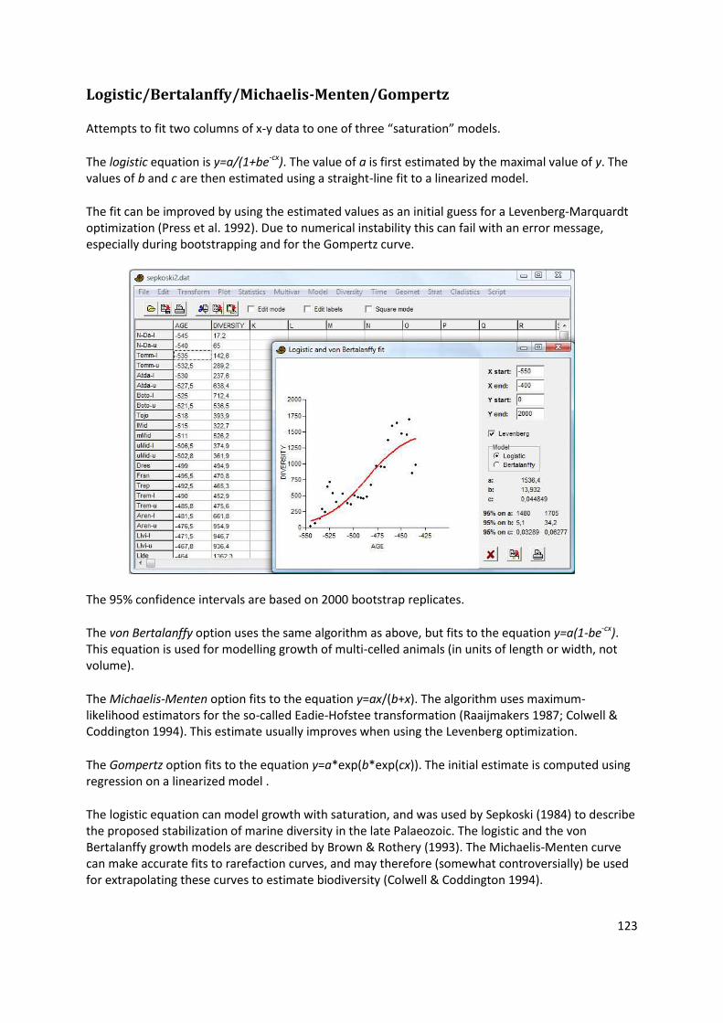
Attempts to fit two columns of x-y data to one of three “saturation” models.
The logistic equation is y=a/(1+be-cx). The value of a is first estimated by the maximal value of y. The values of b and c are then estimated using a straight-line fit to a linearized model.
The fit can be improved by using the estimated values as an initial guess for a Levenberg-Marquardt optimization (Press et al. 1992). Due to numerical instability this can fail with an error message, especially during bootstrapping and for the Gompertz curve.
The 95% confidence intervals are based on 2000 bootstrap replicates.
The von Bertalanffy option uses the same algorithm as above, but fits to the equation y=a(1-be-cx). This equation is used for modelling growth of multi-celled animals (in units of length or width, not volume).
The Michaelis-Menten option fits to the equation y=ax/(b+x). The algorithm uses maximum-likelihood estimators for the so-called Eadie-Hofstee transformation (Raaijmakers 1987; Colwell & Coddington 1994). This estimate usually improves when using the Levenberg optimization.
The Gompertz option fits to the equation y=a*exp(b*exp(cx)). The initial estimate is computed using regression on a linearized model .
The logistic equation can model growth with saturation, and was used by Sepkoski (1984) to describe the proposed stabilization of marine diversity in the late Palaeozoic. The logistic and the von Bertalanffy growth models are described by Brown & Rothery (1993). The Michaelis-Menten curve can make accurate fits to rarefaction curves, and may therefore (somewhat controversially) be used for extrapolating these curves to estimate biodiversity (Colwell & Coddington 1994).

124
The Akaike Information Criterion (AIC) may aid in the selection of model. Lower values for the AIC imply a better fit, adjusted for the number of parameters.
References
Brown, D. & P. Rothery. 1993. Models in biology: mathematics, statistics and computing. John Wiley & Sons.
Colwell, R.K. & J.A. Coddington. 1994. Estimating terrestrial biodiversity through extrapolation. Philosophical Transactions of the Royal Society of London B 345:101-118.
Press, W.H., S.A. Teukolsky, W.T. Vetterling & B.P. Flannery. 1992. Numerical Recipes in C. Cambridge University Press.
Raaijmakers, J.G.W. 1987. Statistical analysis of the Michaelis-Menten equation. Biometrics 43:793-803.
Sepkoski, J.J. 1984. A kinetic model of Phanerozoic taxonomic diversity. Paleobiology 10:246-267.
125
Generalized Linear Model
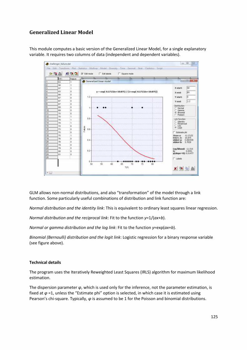
This module computes a basic version of the Generalized Linear Model, for a single explanatory variable. It requires two columns of data (independent and dependent variables).
GLM allows non-normal distributions, and also “transformation” of the model through a link function. Some particularly useful combinations of distribution and link function are:
Normal distribution and the identity link: This is equivalent to ordinary least squares linear regression.
Normal distribution and the reciprocal link: Fit to the function y=1/(ax+b).
Normal or gamma distribution and the log link: Fit to the function y=exp(ax+b).
Binomial (Bernoulli) distribution and the logit link: Logistic regression for a binary response variable (see figure above).
Technical details
The program uses the Iteratively Reweighted Least Squares (IRLS) algorithm for maximum likelihood estimation.
The dispersion parameter φ, which is used only for the inference, not the parameter estimation, is fixed at φ =1, unless the “Estimate phi” option is selected, in which case it is estimated using Pearson’s chi-square. Typically, φ is assumed to be 1 for the Poisson and binomial distributions.

126
The log-likelihood LL is computed from the deviance D by 2
DLL .
The deviance is computed as follows:
Normal: i
iiyD2
Gamma:
i i
ii
i
i yyD
ln2
Bernoulli:
i i
i
i
i
i
i
yy
yyD
1
1ln1ln2 (the first term defined as zero if yi=0)
Poisson:
i
ii
i
i
i yy
yD
ln2
The G statistic is the difference in D between the full model and an additional GLM run where only the intercept is fitted. G is approximately chi-squared with one degree of freedom, giving a significance for the slope.
127
Smoothing spline
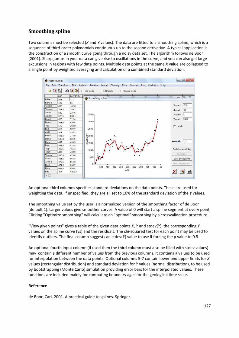
Two columns must be selected (X and Y values). The data are fitted to a smoothing spline, which is a sequence of third-order polynomials continuous up to the second derivative. A typical application is the construction of a smooth curve going through a noisy data set. The algorithm follows de Boor (2001). Sharp jumps in your data can give rise to oscillations in the curve, and you can also get large excursions in regions with few data points. Multiple data points at the same X value are collapsed to a single point by weighted averaging and calculation of a combined standard deviation.
An optional third columns specifies standard deviations on the data points. These are used for weighting the data. If unspecified, they are all set to 10% of the standard deviation of the Y values.
The smoothing value set by the user is a normalized version of the smoothing factor of de Boor (default 1). Larger values give smoother curves. A value of 0 will start a spline segment at every point. Clicking "Optimize smoothing" will calculate an "optimal" smoothing by a crossvalidation procedure.
"View given points" gives a table of the given data points X, Y and stdev(Y), the corresponding Y values on the spline curve (ys) and the residuals. The chi-squared test for each point may be used to identify outliers. The final column suggests an stdev(Y) value to use if forcing the p value to 0.5.
An optional fourth input column (if used then the third column must also be filled with stdev values) may contain a different number of values from the previous columns. It contains X values to be used for interpolation between the data points. Optional columns 5-7 contain lower and upper limits for X values (rectangular distribution) and standard deviation for Y values (normal distribution), to be used by bootstrapping (Monte Carlo) simulation providing error bars for the interpolated values. These functions are included mainly for computing boundary ages for the geological time scale.
Reference
de Boor, Carl. 2001. A practical guide to splines. Springer.
128
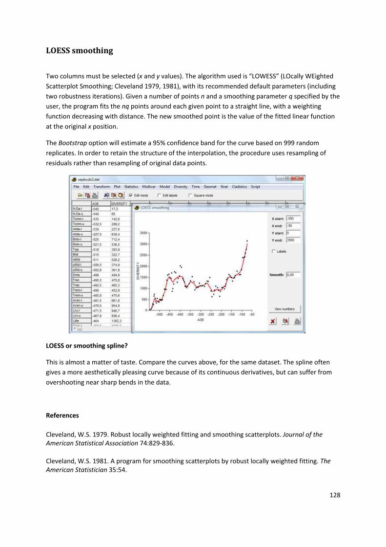
LOESS smoothing
Two columns must be selected (x and y values). The algorithm used is “LOWESS” (LOcally WEighted
Scatterplot Smoothing; Cleveland 1979, 1981), with its recommended default parameters (including
two robustness iterations). Given a number of points n and a smoothing parameter q specified by the
user, the program fits the nq points around each given point to a straight line, with a weighting
function decreasing with distance. The new smoothed point is the value of the fitted linear function
at the original x position.
The Bootstrap option will estimate a 95% confidence band for the curve based on 999 random
replicates. In order to retain the structure of the interpolation, the procedure uses resampling of
residuals rather than resampling of original data points.
LOESS or smoothing spline?
This is almost a matter of taste. Compare the curves above, for the same dataset. The spline often
gives a more aesthetically pleasing curve because of its continuous derivatives, but can suffer from
overshooting near sharp bends in the data.
References
Cleveland, W.S. 1979. Robust locally weighted fitting and smoothing scatterplots. Journal of the American Statistical Association 74:829-836.
Cleveland, W.S. 1981. A program for smoothing scatterplots by robust locally weighted fitting. The American Statistician 35:54.
129
Mixture analysis
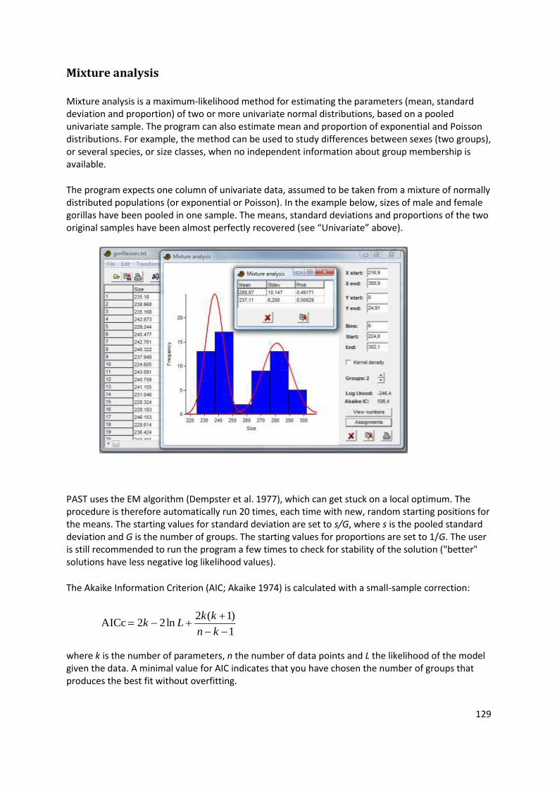
Mixture analysis is a maximum-likelihood method for estimating the parameters (mean, standard deviation and proportion) of two or more univariate normal distributions, based on a pooled univariate sample. The program can also estimate mean and proportion of exponential and Poisson distributions. For example, the method can be used to study differences between sexes (two groups), or several species, or size classes, when no independent information about group membership is available.
The program expects one column of univariate data, assumed to be taken from a mixture of normally distributed populations (or exponential or Poisson). In the example below, sizes of male and female gorillas have been pooled in one sample. The means, standard deviations and proportions of the two original samples have been almost perfectly recovered (see “Univariate” above).
PAST uses the EM algorithm (Dempster et al. 1977), which can get stuck on a local optimum. The procedure is therefore automatically run 20 times, each time with new, random starting positions for the means. The starting values for standard deviation are set to s/G, where s is the pooled standard deviation and G is the number of groups. The starting values for proportions are set to 1/G. The user is still recommended to run the program a few times to check for stability of the solution ("better" solutions have less negative log likelihood values).
The Akaike Information Criterion (AIC; Akaike 1974) is calculated with a small-sample correction:
1
)1(2ln22AICc
kn
kkLk
where k is the number of parameters, n the number of data points and L the likelihood of the model given the data. A minimal value for AIC indicates that you have chosen the number of groups that produces the best fit without overfitting.
130
It is possible to assign each of the data points to one of the groups with a maximum likelihood approach. This can be used as a non-hierarchical clustering method for univariate data. The “Assignments” button will open a window where the value of each probability density function is given for each data point. The data point can be assigned to the group that shows the largest value.
Missing data: Supported by deletion.
References
Akaike, H. 1974. A new look at the statistical model identification. IEEE Transactions on Automatic Control 19: 716-723.
Dempster, A.P., Laird, N.M. & Rubin, D.B. 1977. Maximum likelihood from incomplete data via the EM algorithm". Journal of the Royal Statistical Society, Series B 39:1-38.
131
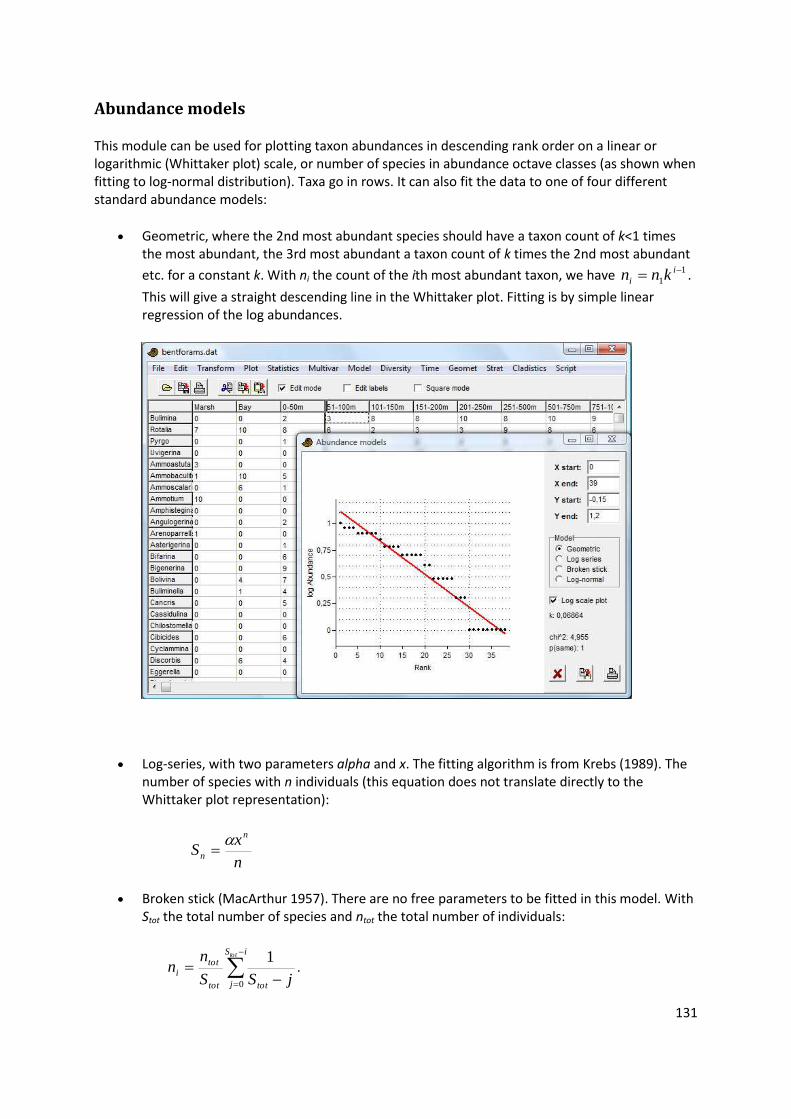
Abundance models
This module can be used for plotting taxon abundances in descending rank order on a linear or logarithmic (Whittaker plot) scale, or number of species in abundance octave classes (as shown when fitting to log-normal distribution). Taxa go in rows. It can also fit the data to one of four different standard abundance models:
Geometric, where the 2nd most abundant species should have a taxon count of k<1 times the most abundant, the 3rd most abundant a taxon count of k times the 2nd most abundant
etc. for a constant k. With ni the count of the ith most abundant taxon, we have 1
1
i
i knn .
This will give a straight descending line in the Whittaker plot. Fitting is by simple linear regression of the log abundances.
Log-series, with two parameters alpha and x. The fitting algorithm is from Krebs (1989). The number of species with n individuals (this equation does not translate directly to the Whittaker plot representation):
n
xS
n
n
Broken stick (MacArthur 1957). There are no free parameters to be fitted in this model. With Stot the total number of species and ntot the total number of individuals:
iS
j tottot
tot
i
tot
jSS
nn
0
1.
132
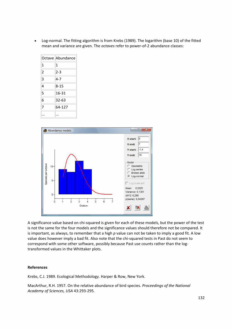
Log-normal. The fitting algorithm is from Krebs (1989). The logarithm (base 10) of the fitted mean and variance are given. The octaves refer to power-of-2 abundance classes:
Octave Abundance
1 1
2 2-3
3 4-7
4 8-15
5 16-31
6 32-63
7 64-127
... ...
A significance value based on chi-squared is given for each of these models, but the power of the test is not the same for the four models and the significance values should therefore not be compared. It is important, as always, to remember that a high p value can not be taken to imply a good fit. A low value does however imply a bad fit. Also note that the chi-squared tests in Past do not seem to correspond with some other software, possibly because Past use counts rather than the log-transformed values in the Whittaker plots.
References
Krebs, C.J. 1989. Ecological Methodology. Harper & Row, New York.
MacArthur, R.H. 1957. On the relative abundance of bird species. Proceedings of the National Academy of Sciences, USA 43:293-295.
133
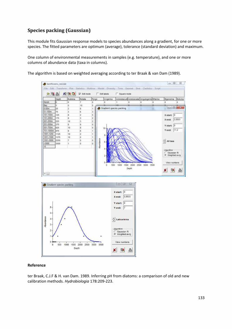
Species packing (Gaussian)
This module fits Gaussian response models to species abundances along a gradient, for one or more species. The fitted parameters are optimum (average), tolerance (standard deviation) and maximum.
One column of environmental measurements in samples (e.g. temperature), and one or more columns of abundance data (taxa in columns).
The algorithm is based on weighted averaging according to ter Braak & van Dam (1989).
Reference
ter Braak, C.J.F & H. van Dam. 1989. Inferring pH from diatoms: a comparison of old and new calibration methods. Hydrobiologia 178:209-223.
134
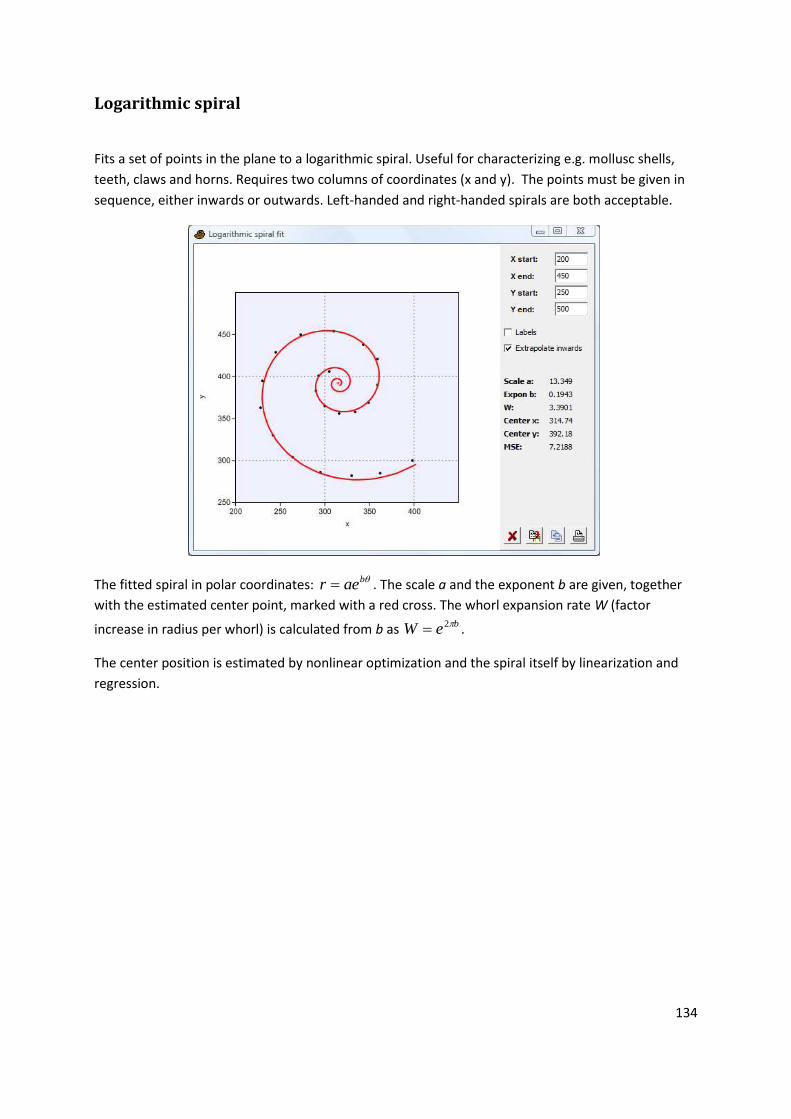
Logarithmic spiral
Fits a set of points in the plane to a logarithmic spiral. Useful for characterizing e.g. mollusc shells,
teeth, claws and horns. Requires two columns of coordinates (x and y). The points must be given in
sequence, either inwards or outwards. Left-handed and right-handed spirals are both acceptable.
The fitted spiral in polar coordinates: baer . The scale a and the exponent b are given, together
with the estimated center point, marked with a red cross. The whorl expansion rate W (factor
increase in radius per whorl) is calculated from b as beW 2 .
The center position is estimated by nonlinear optimization and the spiral itself by linearization and
regression.

135
Diversity menu
Diversity indices
These statistics apply to association data, where number of individuals are tabulated in rows (taxa) and possibly several columns (associations). The available statistics are as follows, for each association:
Number of taxa (S)
Total number of individuals (n)
Dominance = 1-Simpson index. Ranges from 0 (all taxa are equally present) to 1 (one taxon dominates the community completely).
i
i
n
nD
2
where ni is number of individuals of taxon i.
Simpson index 1-D. Measures 'evenness' of the community from 0 to 1. Note the confusion in the literature: Dominance and Simpson indices are often interchanged!
Shannon index (entropy). A diversity index, taking into account the number of individuals as well as number of taxa. Varies from 0 for communities with only a single taxon to high values for communities with many taxa, each with few individuals.
i
ii
n
n
n
nH ln
Buzas and Gibson's evenness: eH/S
Brillouin’s index:
n
nn
HB i
i
!ln!ln
Menhinick's richness index: n
S
Margalef's richness index: (S-1) / ln(n)
Equitability. Shannon diversity divided by the logarithm of number of taxa. This measures the evenness with which individuals are divided among the taxa present.
Fisher's alpha - a diversity index, defined implicitly by the formula S=a*ln(1+n/a) where S is number of taxa, n is number of individuals and a is the Fisher's alpha.
Berger-Parker dominance: simply the number of individuals in the dominant taxon relative to n.
136
Chao1, bias corrected: An estimate of total species richness. Chao1 = S + F1(F1 - 1) / (2 (F2 + 1)), where F1 is the number of singleton species and F2 the number of doubleton species.
Many of these indices are explained in Harper (1999).
Approximate confidence intervals for all these indices can be computed with a bootstrap procedure. 1000 random samples are produced (200 prior to version 0.87b), each with the same total number of individuals as in each original sample. The random samples are taken from the total, pooled data set (all columns). For each individual in the random sample, the taxon is chosen with probabilities according to the original, pooled abundances. A 95 percent confidence interval is then calculated. Note that the diversity in the replicates will often be less than, and never larger than, the pooled diversity in the total data set.
Since these confidence intervals are all computed with respect to the pooled data set, they do not represent confidence intervals for the individual samples. They are mainly useful for identifying samples where the given diversity index falls outside the confidence interval. Bootstrapped comparison of diversity indices in two samples is provided in the Compare diversities module.
Reference
Harper, D.A.T. (ed.). 1999. Numerical Palaeobiology. John Wiley & Sons.
137
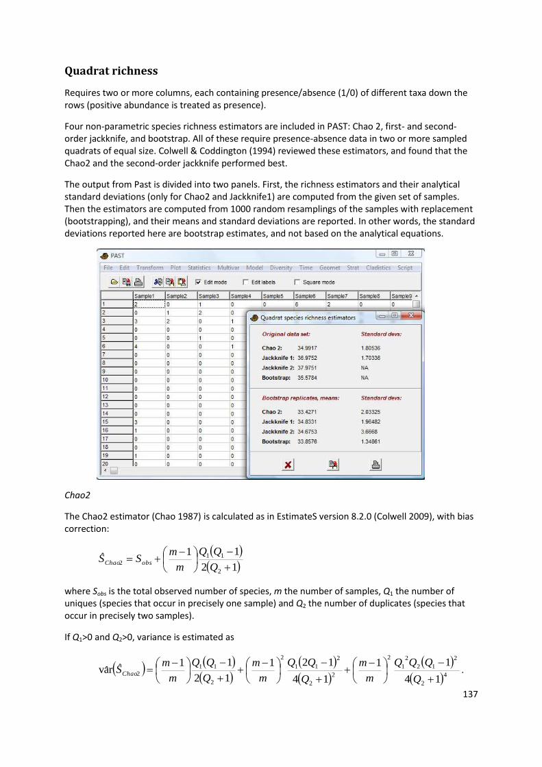
Quadrat richness
Requires two or more columns, each containing presence/absence (1/0) of different taxa down the rows (positive abundance is treated as presence).
Four non-parametric species richness estimators are included in PAST: Chao 2, first- and second-order jackknife, and bootstrap. All of these require presence-absence data in two or more sampled quadrats of equal size. Colwell & Coddington (1994) reviewed these estimators, and found that the Chao2 and the second-order jackknife performed best.
The output from Past is divided into two panels. First, the richness estimators and their analytical standard deviations (only for Chao2 and Jackknife1) are computed from the given set of samples. Then the estimators are computed from 1000 random resamplings of the samples with replacement (bootstrapping), and their means and standard deviations are reported. In other words, the standard deviations reported here are bootstrap estimates, and not based on the analytical equations.
Chao2
The Chao2 estimator (Chao 1987) is calculated as in EstimateS version 8.2.0 (Colwell 2009), with bias correction:
12
11ˆ
2
112
Q
m
mSS obsChao
where Sobs is the total observed number of species, m the number of samples, Q1 the number of uniques (species that occur in precisely one sample) and Q2 the number of duplicates (species that occur in precisely two samples).
If Q1>0 and Q2>0, variance is estimated as
4
2
2
12
2
1
2
2
2
2
11
2
2
112
14
11
14
121
12
11ˆrav
Q
QQQ
m
m
Q
m
m
Q
m
mSChao .
138
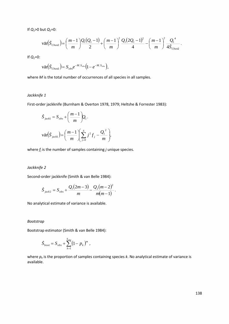
If Q1>0 but Q2=0:
2
4
1
22
11
2
112 ˆ4
1
4
121
2
11ˆrav
Chao
ChaoS
Q
m
mQQ
m
mQQ
m
mS
.
If Q1=0:
obsobs SMSM
obsChao eeSS
1ˆrav 2 ,
where M is the total number of occurrences of all species in all samples.
Jackknife 1
First-order jackknife (Burnham & Overton 1978, 1979; Heltshe & Forrester 1983):
11
1ˆ Q
m
mSS obsjack
.
S
j
jjackm
Qfj
m
mS
0
2
12
1
1ˆrav ,
where fj is the number of samples containing j unique species.
Jackknife 2
Second-order jackknife (Smith & van Belle 1984):
1
232ˆ
2
212
mm
mQ
m
mQSS obsjack .
No analytical estimate of variance is available.
Bootstrap
Bootstrap estimator (Smith & van Belle 1984):
obsS
k
m
kobsboot pSS1
1ˆ ,
where pk is the proportion of samples containing species k. No analytical estimate of variance is available.
139
References
Burnham, K.P. & W.S. Overton. 1978. Estimation of the size of a closed population when capture probabilities vary among animals. Biometrika 65:623-633.
Burnham, K.P. & W.S. Overton. 1979. Robust estimation of population size when capture probabilities vary among animals. Ecology 60:927-936.
Chao, A. 1987. Estimating the population size for capture-recapture data with unequal catchability. Biometrics 43, 783-791.
Colwell, R.K. & J.A. Coddington. 1994. Estimating terrestrial biodiversity through extrapolation. Philosophical Transactions of the Royal Society (Series B) 345:101-118.
Heltshe, J. & N.E. Forrester. 1983. Estimating species richness using the jackknife procedure. Biometrics 39:1-11.
Smith, E.P. & G. van Belle. 1984. Nonparametric estimation of species richness. Biometrics 40:119-129.
140
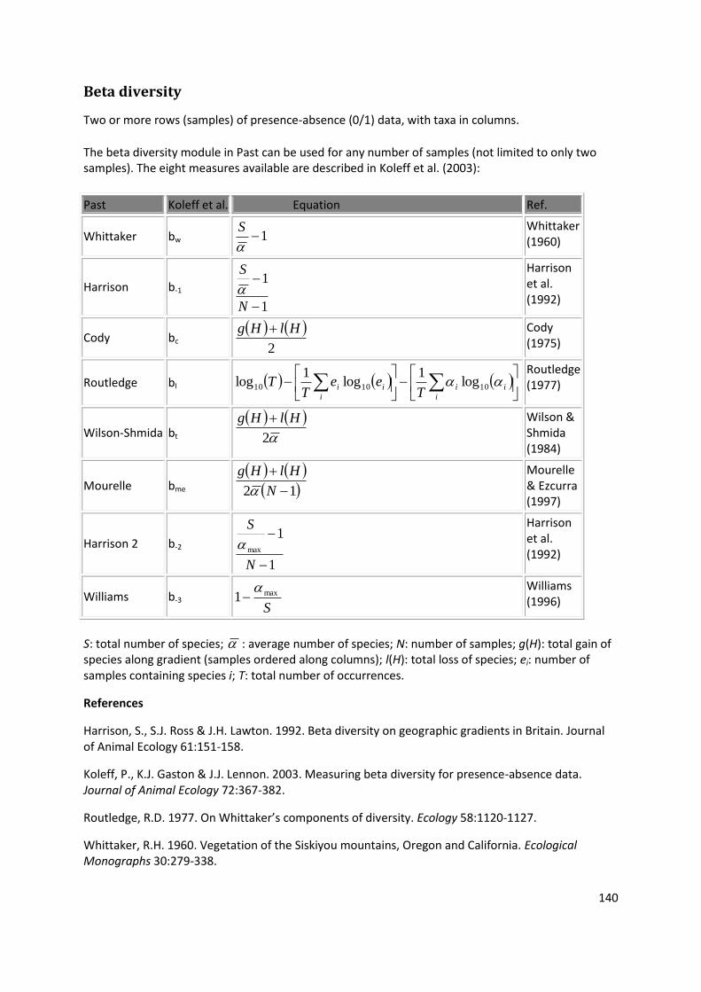
Beta diversity
Two or more rows (samples) of presence-absence (0/1) data, with taxa in columns.
The beta diversity module in Past can be used for any number of samples (not limited to only two samples). The eight measures available are described in Koleff et al. (2003):
Past Koleff et al. Equation Ref.
Whittaker bw 1
S
Whittaker (1960)
Harrison b-1
1
1
N
S
Harrison et al. (1992)
Cody bc
2
HlHg
Cody (1975)
Routledge bI
i
ii
i
iiT
eeT
T 101010 log1
log1
log Routledge (1977)
Wilson-Shmida bt
2
HlHg
Wilson & Shmida (1984)
Mourelle bme
12
N
HlHg
Mourelle & Ezcurra (1997)
Harrison 2 b-2
1
1max
N
S
Harrison et al. (1992)
Williams b-3 S
max1
Williams (1996)
S: total number of species; : average number of species; N: number of samples; g(H): total gain of species along gradient (samples ordered along columns); l(H): total loss of species; ei: number of samples containing species i; T: total number of occurrences.
References
Harrison, S., S.J. Ross & J.H. Lawton. 1992. Beta diversity on geographic gradients in Britain. Journal of Animal Ecology 61:151-158.
Koleff, P., K.J. Gaston & J.J. Lennon. 2003. Measuring beta diversity for presence-absence data. Journal of Animal Ecology 72:367-382.
Routledge, R.D. 1977. On Whittaker’s components of diversity. Ecology 58:1120-1127.
Whittaker, R.H. 1960. Vegetation of the Siskiyou mountains, Oregon and California. Ecological Monographs 30:279-338.
141
Taxonomic distinctness
One or more columns, each containing counts of individuals of different taxa down the rows. In addition, the leftmost row(s) must contain names of genera/families etc. (see below).
Taxonomic diversity and taxonomic distinctness as defined by Clarke & Warwick (1998), including confidence intervals computed from 200 random replicates taken from the pooled data set (all columns). Note that the "global list" of Clarke & Warwick is not entered directly, but is calculated internally by pooling (summing) the given samples.
These indices depend on taxonomic information also above the species level, which has to be entered for each species as follows. Species names go in the name column (leftmost, fixed column), genus names in column 1, family in column 2 etc. (of course you can substitute for other taxonomic levels as long as they are in ascending order). Species counts follow in the columns thereafter. The program will ask for the number of columns containing taxonomic information above the species level.
For presence-absence data, taxonomic diversity and distinctness will be valid but equal to each other.
Taxonomic distinctness in one sample is given by (note other, equivalent forms exist):
ji i
iiji
ji
jiij
xxxx
xxw
21,
where the wij are weights such that wij = 0 if i and j are the same species, wij = 1 if they are the same genus, etc. The x are the abundances.
Taxonomic distinctness:
ji
ji
ji
jiij
xx
xxw* .
Reference
Clarke, K.R. & Warwick, R.M. 1998. A taxonomic distinctness index and its statistical properties. Journal of Applied Ecology 35:523-531.
142
Individual rarefaction
For comparing taxonomical diversity in samples of different sizes. Requires one or more columns of counts of individuals of different taxa (each column must have the same number of values). When comparing samples: Samples should be taxonomically similar, obtained using standardised sampling and taken from similar 'habitat'.
Given one or more columns of abundance data for a number of taxa, this module estimates how many taxa you would expect to find in a sample with a smaller total number of individuals. With this method, you can compare the number of taxa in samples of different size. Using rarefaction analysis on your largest sample, you can read out the number of expected taxa for any smaller sample size (including that of the smallest sample). The algorithm is from Krebs (1989), using a log Gamma function for computing combinatorial terms. An example application in paleontology can be found in Adrain et al. (2000).
Let N be the total number of individuals in the sample, s the total number of species, and Ni the number of individuals of species number i. The expected number of species E(Sn) in a sample of size n and the variance V(Sn) are then given by
s
i
i
n
n
N
n
NN
SE1
1
s
j
j
i
jiji
s
i
ii
n
n
N
n
N
n
NN
n
NN
n
N
n
NNN
n
N
n
NN
n
N
n
NN
SV
2
1
1
1
2
1
Standard errors (square roots of variances) are given by the program. In the graphical plot, these standard errors are converted to 95 percent confidence intervals.
References
Adrain, J.M., S.R. Westrop & D.E. Chatterton. 2000. Silurian trilobite alpha diversity and the end-Ordovician mass extinction. Paleobiology 26:625-646.
Krebs, C.J. 1989. Ecological Methodology. Harper & Row, New York.
143
Sample rarefaction (Mao tau)
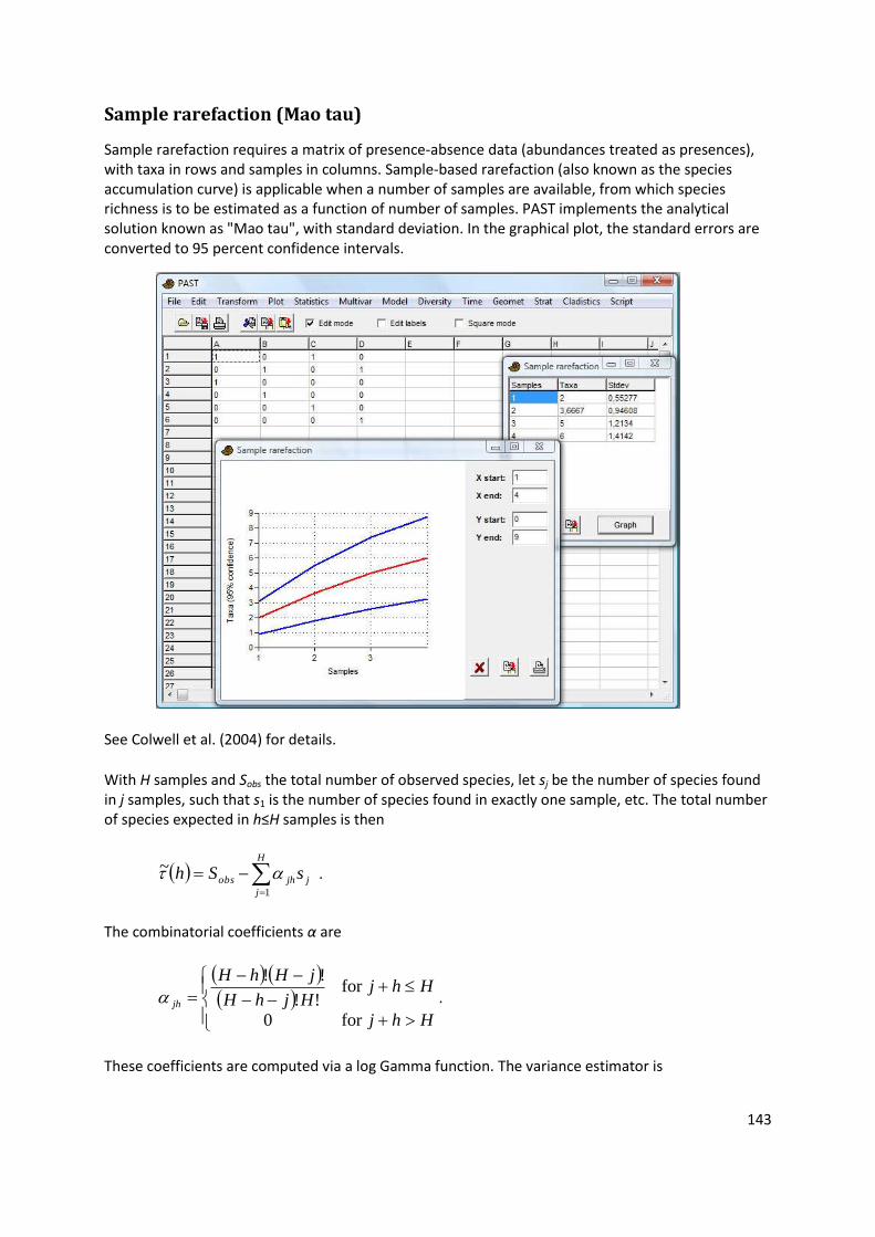
Sample rarefaction requires a matrix of presence-absence data (abundances treated as presences), with taxa in rows and samples in columns. Sample-based rarefaction (also known as the species accumulation curve) is applicable when a number of samples are available, from which species richness is to be estimated as a function of number of samples. PAST implements the analytical solution known as "Mao tau", with standard deviation. In the graphical plot, the standard errors are converted to 95 percent confidence intervals.
See Colwell et al. (2004) for details.
With H samples and Sobs the total number of observed species, let sj be the number of species found in j samples, such that s1 is the number of species found in exactly one sample, etc. The total number of species expected in h≤H samples is then
H
j
jjhobs sSh1
~ .
The combinatorial coefficients α are
Hhj
HhjHjhH
jHhH
jh
for 0
for !!
!!
.
These coefficients are computed via a log Gamma function. The variance estimator is
144
H
j
jjhS
hs
1
222
~
~1~
,
where S~
is an estimator for the unknown total species richness. Following Colwell et al. (2004), a Chao2-type estimator is used. For s2>0,
2
2
1
2
1~
Hs
sHSS obs
.
For s2=0,
12
11~
2
11
sH
ssHSS obs .
For modeling and extrapolating the curve using the Michaelis-Menten equation, use the Copy Data button, paste to a new Past spreadsheet, and use the fitting module in the Model menu.
Reference
Colwell, R.K., C.X. Mao & J. Chang. 2004. Interpolating, extrapolating, and comparing incidence-based species accumulation curves. Ecology 85:2717-2727.
145
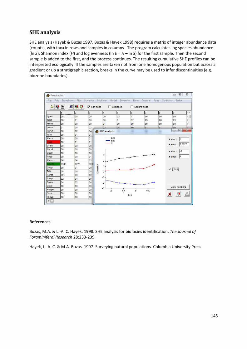
SHE analysis
SHE analysis (Hayek & Buzas 1997, Buzas & Hayek 1998) requires a matrix of integer abundance data (counts), with taxa in rows and samples in columns. The program calculates log species abundance (ln S), Shannon index (H) and log evenness (ln E = H – ln S) for the first sample. Then the second sample is added to the first, and the process continues. The resulting cumulative SHE profiles can be interpreted ecologically. If the samples are taken not from one homogenous population but across a gradient or up a stratigraphic section, breaks in the curve may be used to infer discontinuities (e.g. biozone boundaries).
References
Buzas, M.A. & L.-A. C. Hayek. 1998. SHE analysis for biofacies identification. The Journal of Foraminiferal Research 28:233-239.
Hayek, L.-A. C. & M.A. Buzas. 1997. Surveying natural populations. Columbia University Press.

146
Compare diversities
Expects two columns of abundance data with taxa down the rows.This module computes a number of diversity indices for two samples, and then compares the diversities using two different randomisation procedures as follows.
Bootstrapping The two samples A and B are pooled. 1000 random pairs of samples (Ai,Bi) are then taken from this pool, with the same numbers of individuals as in the original two samples. For each replicate pair, the diversity indices div(Ai) and div(Bi) are computed. The number of times |div(Ai)-div(Bi)| exceeds or equals |div(A)-div(B)| indicates the probability that the observed difference could have occurred by random sampling from one parent population as estimated by the pooled sample.
A small probability value p(same) then indicates a significant difference in diversity index between the two samples.
Permutation 1000 random matrices with two columns (samples) are generated, each with the same row and column totals as in the original data matrix. The p value is computed as for the bootstrap test.
147
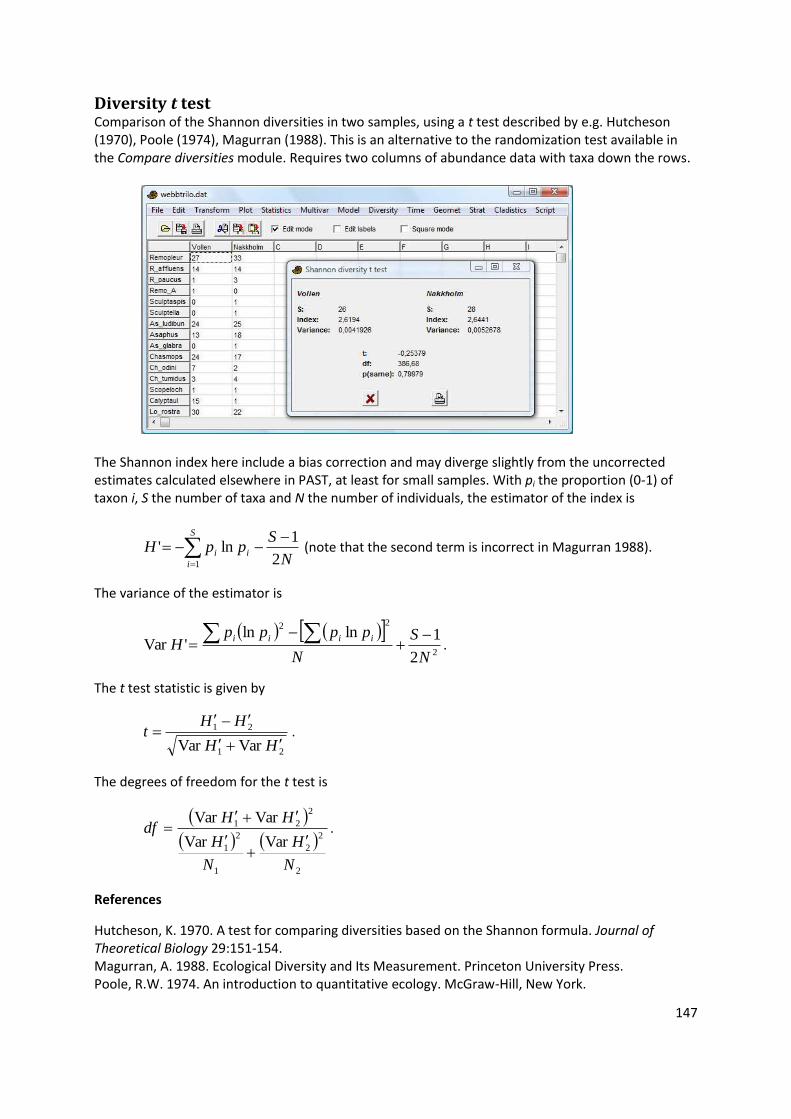
Diversity t test Comparison of the Shannon diversities in two samples, using a t test described by e.g. Hutcheson (1970), Poole (1974), Magurran (1988). This is an alternative to the randomization test available in the Compare diversities module. Requires two columns of abundance data with taxa down the rows.
The Shannon index here include a bias correction and may diverge slightly from the uncorrected estimates calculated elsewhere in PAST, at least for small samples. With pi the proportion (0-1) of taxon i, S the number of taxa and N the number of individuals, the estimator of the index is
S
i
iiN
SppH
1 2
1ln' (note that the second term is incorrect in Magurran 1988).
The variance of the estimator is
2
22
2
1lnln'Var
N
S
N
ppppH
iiii
.
The t test statistic is given by
21
21
VarVar HH
HHt
.
The degrees of freedom for the t test is
2
2
2
1
2
1
2
21
VarVar
VarVar
N
H
N
H
HHdf
.
References
Hutcheson, K. 1970. A test for comparing diversities based on the Shannon formula. Journal of Theoretical Biology 29:151-154. Magurran, A. 1988. Ecological Diversity and Its Measurement. Princeton University Press. Poole, R.W. 1974. An introduction to quantitative ecology. McGraw-Hill, New York.
148
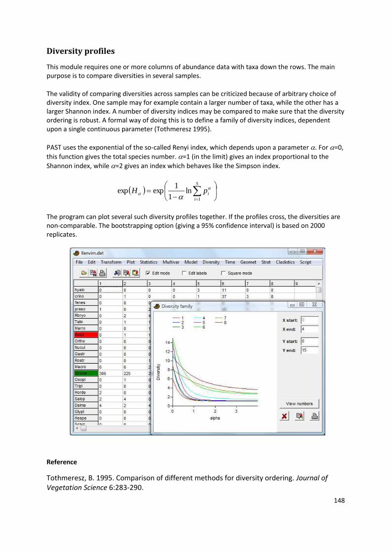
Diversity profiles
This module requires one or more columns of abundance data with taxa down the rows. The main purpose is to compare diversities in several samples.
The validity of comparing diversities across samples can be criticized because of arbitrary choice of diversity index. One sample may for example contain a larger number of taxa, while the other has a larger Shannon index. A number of diversity indices may be compared to make sure that the diversity ordering is robust. A formal way of doing this is to define a family of diversity indices, dependent upon a single continuous parameter (Tothmeresz 1995).
PAST uses the exponential of the so-called Renyi index, which depends upon a parameter . For =0,
this function gives the total species number. =1 (in the limit) gives an index proportional to the
Shannon index, while =2 gives an index which behaves like the Simpson index.
S
i
ipH1
ln1
1expexp
The program can plot several such diversity profiles together. If the profiles cross, the diversities are non-comparable. The bootstrapping option (giving a 95% confidence interval) is based on 2000 replicates.
Reference
Tothmeresz, B. 1995. Comparison of different methods for diversity ordering. Journal of Vegetation Science 6:283-290.
149
Time series menu
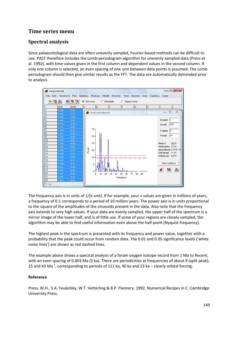
Spectral analysis
Since palaeontological data are often unevenly sampled, Fourier-based methods can be difficult to use. PAST therefore includes the Lomb periodogram algorithm for unevenly sampled data (Press et al. 1992), with time values given in the first column and dependent values in the second column. If only one column is selected, an even spacing of one unit between data points is assumed. The Lomb periodogram should then give similar results as the FFT. The data are automatically detrended prior to analysis.
The frequency axis is in units of 1/(x unit). If for example, your x values are given in millions of years, a frequency of 0.1 corresponds to a period of 10 million years. The power axis is in units proportional to the square of the amplitudes of the sinusoids present in the data. Also note that the frequency axis extends to very high values. If your data are evenly sampled, the upper half of the spectrum is a mirror image of the lower half, and is of little use. If some of your regions are closely sampled, the algorithm may be able to find useful information even above the half-point (Nyquist frequency).
The highest peak in the spectrum is presented with its frequency and power value, together with a probability that the peak could occur from random data. The 0.01 and 0.05 significance levels ('white noise lines') are shown as red dashed lines.
The example above shows a spectral analysis of a foram oxygen isotope record from 1 Ma to Recent, with an even spacing of 0.003 Ma (3 ka). There are periodicities at frequencies of about 9 (split peak), 25 and 43 Ma-1, corresponding to periods of 111 ka, 40 ka and 23 ka – clearly orbital forcing.
Reference
Press, W.H., S.A. Teukolsky, W.T. Vetterling & B.P. Flannery. 1992. Numerical Recipes in C. Cambridge University Press.
150
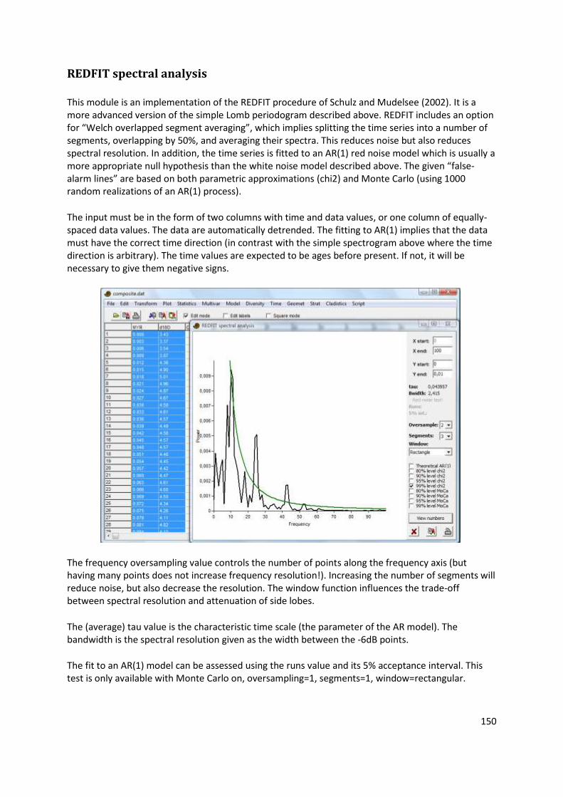
REDFIT spectral analysis
This module is an implementation of the REDFIT procedure of Schulz and Mudelsee (2002). It is a more advanced version of the simple Lomb periodogram described above. REDFIT includes an option for “Welch overlapped segment averaging”, which implies splitting the time series into a number of segments, overlapping by 50%, and averaging their spectra. This reduces noise but also reduces spectral resolution. In addition, the time series is fitted to an AR(1) red noise model which is usually a more appropriate null hypothesis than the white noise model described above. The given “false-alarm lines” are based on both parametric approximations (chi2) and Monte Carlo (using 1000 random realizations of an AR(1) process).
The input must be in the form of two columns with time and data values, or one column of equally-spaced data values. The data are automatically detrended. The fitting to AR(1) implies that the data must have the correct time direction (in contrast with the simple spectrogram above where the time direction is arbitrary). The time values are expected to be ages before present. If not, it will be necessary to give them negative signs.
The frequency oversampling value controls the number of points along the frequency axis (but having many points does not increase frequency resolution!). Increasing the number of segments will reduce noise, but also decrease the resolution. The window function influences the trade-off between spectral resolution and attenuation of side lobes.
The (average) tau value is the characteristic time scale (the parameter of the AR model). The bandwidth is the spectral resolution given as the width between the -6dB points.
The fit to an AR(1) model can be assessed using the runs value and its 5% acceptance interval. This test is only available with Monte Carlo on, oversampling=1, segments=1, window=rectangular.
151
In addition to a fixed set of false-alarm levels (80%, 90%, 95% and 99%), the program also reports a “critical” false-alarm level (False-al) that depends on the segment length (Thomson 1990).
Important: Because of long computation time, the Monte Carlo simulation is not run by default, and the Monte Carlo false-alarm levels are therefore not available. When the Monte Carlo option is enabled, the given spectrum may change slightly because the Monte Carlo results are then used to compute a “bias-corrected” version (see Schulz and Mudelsee 2002).
References
Schulz, M. & M. Mudelsee. 2002. REDFIT: estimating red-noise spectra directly from unevenly spaced paleoclimatic time series. Computers & Geosciences 28:421-426.
Thomson, D.J. 1990. Time series analysis of Holocene climate data. Philosophical Transactions of the Royal Society of London, Series A 330:601-616.
152
Multitaper spectral analysis
In traditional spectral estimation, the data are often “windowed” (multiplied with a bell-shaped function) in order to reduce spectral leakage. In the multitaper method, several different (orthogonal) window functions are applied, and the results combined. The resulting spectrum has low leakage, low variance, and retains information contained in the beginning and end of the time series. In addition, statistical testing can take advantage of the multiple spectral estimates. One possible disadvantage is reduced spectral resolution.
The multitaper method requires evenly spaced data, given in one column.
The implementation in Past is based on the code of Lees & Park (1995). The multitaper spectrum can be compared with a simple periodogram (FFT with a 10% cosine window) and a smoothed periodogram. The number of tapers (NWIN) can be set to 3, 4 or 5, for different tradeoffs between variance reduction and resolution. The “time-bandwidth product” p is fixed at 3.0.
The F test for significance of periodicity follows Lees & Park (1995). The 0.05 and 0.01 significance levels are shown as horizontal lines, based on 2 and 2*NWIN-2 degrees of freedom.
The data are zero-padded to the second lowest power of 2 above the length of the sequence. This is required to reproduce the test results given by Lees & Park (1995).
Reference
Lees, J.M. & J. Park. 1995. Multiple-taper spectral analysis: a stand-alone C-subroutine. Computers & Geosciences 21:199-236.
153
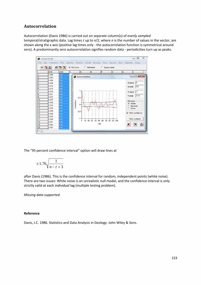
Autocorrelation
Autocorrelation (Davis 1986) is carried out on separate column(s) of evenly sampled temporal/stratigraphic data. Lag times τ up to n/2, where n is the number of values in the vector, are shown along the x axis (positive lag times only - the autocorrelation function is symmetrical around zero). A predominantly zero autocorrelation signifies random data - periodicities turn up as peaks.
The "95 percent confidence interval" option will draw lines at
3
176.1
n
after Davis (1986). This is the confidence interval for random, independent points (white noise). There are two issues: White noise is an unrealistic null model, and the confidence interval is only strictly valid at each individual lag (multiple testing problem).
Missing data supported.
Reference
Davis, J.C. 1986. Statistics and Data Analysis in Geology. John Wiley & Sons.
154
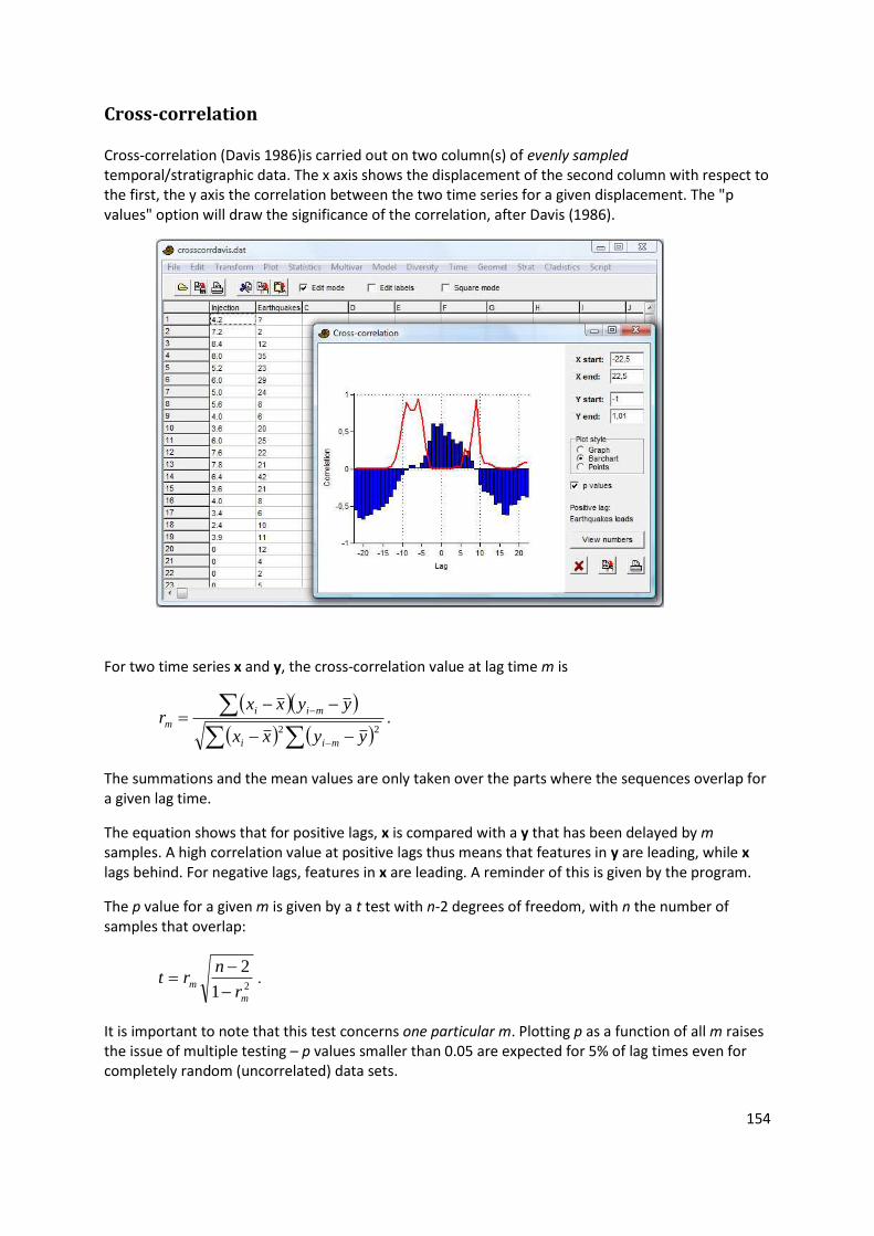
Cross-correlation
Cross-correlation (Davis 1986)is carried out on two column(s) of evenly sampled temporal/stratigraphic data. The x axis shows the displacement of the second column with respect to the first, the y axis the correlation between the two time series for a given displacement. The "p values" option will draw the significance of the correlation, after Davis (1986).
For two time series x and y, the cross-correlation value at lag time m is
22yyxx
yyxxr
mii
mii
m .
The summations and the mean values are only taken over the parts where the sequences overlap for a given lag time.
The equation shows that for positive lags, x is compared with a y that has been delayed by m samples. A high correlation value at positive lags thus means that features in y are leading, while x lags behind. For negative lags, features in x are leading. A reminder of this is given by the program.
The p value for a given m is given by a t test with n-2 degrees of freedom, with n the number of samples that overlap:
21
2
m
mr
nrt
.
It is important to note that this test concerns one particular m. Plotting p as a function of all m raises the issue of multiple testing – p values smaller than 0.05 are expected for 5% of lag times even for completely random (uncorrelated) data sets.

155
In the example above, the “earthquakes” data seem to lag behind the “injection” data with a delay of 0-2 samples (months in this case), where the correlation values are highest. The p values (red curve) indicates significance at these lags. Curiously, there also seems to be significance for negative correlation at large positive and negative lags.
Missing data supported.
Reference
Davis, J.C. 1986. Statistics and Data Analysis in Geology. John Wiley & Sons.
156
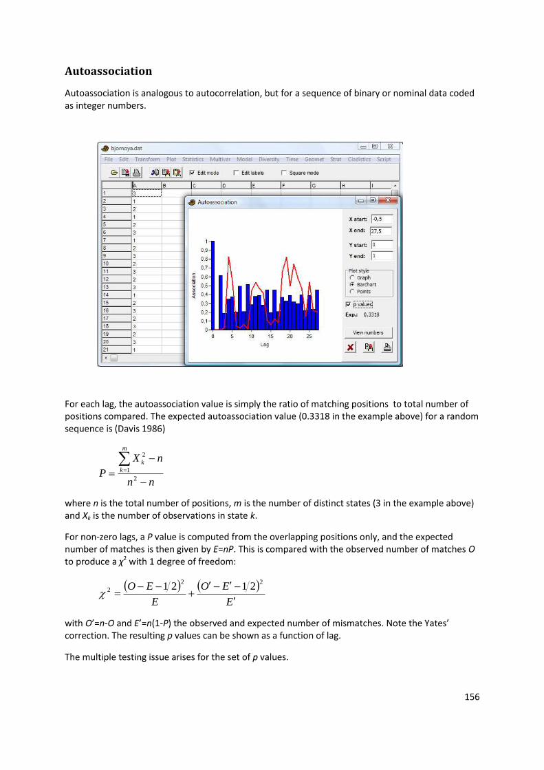
Autoassociation
Autoassociation is analogous to autocorrelation, but for a sequence of binary or nominal data coded as integer numbers.
For each lag, the autoassociation value is simply the ratio of matching positions to total number of positions compared. The expected autoassociation value (0.3318 in the example above) for a random sequence is (Davis 1986)
nn
nX
P
m
k
k
2
1
2
where n is the total number of positions, m is the number of distinct states (3 in the example above) and Xk is the number of observations in state k.
For non-zero lags, a P value is computed from the overlapping positions only, and the expected number of matches is then given by E=nP. This is compared with the observed number of matches O to produce a χ2 with 1 degree of freedom:
E
EO
E
EO
22
2 2121
with O’=n-O and E’=n(1-P) the observed and expected number of mismatches. Note the Yates’ correction. The resulting p values can be shown as a function of lag.
The multiple testing issue arises for the set of p values.

157
The test above is not strictly valid for “transition” sequences where repetitions are not allowed (the sequence in the example above is of this type). In this case, select the “No repetitions” option. The p values will then be computed by an exact test, where all possible permutations without repeats are computed and the autoassociation compared with the original values. This test will take a long time to run for n>30, and the option is not available for n>40.
Missing data supported.
Reference
Davis, J.C. 1986. Statistics and Data Analysis in Geology. John Wiley & Sons.
158
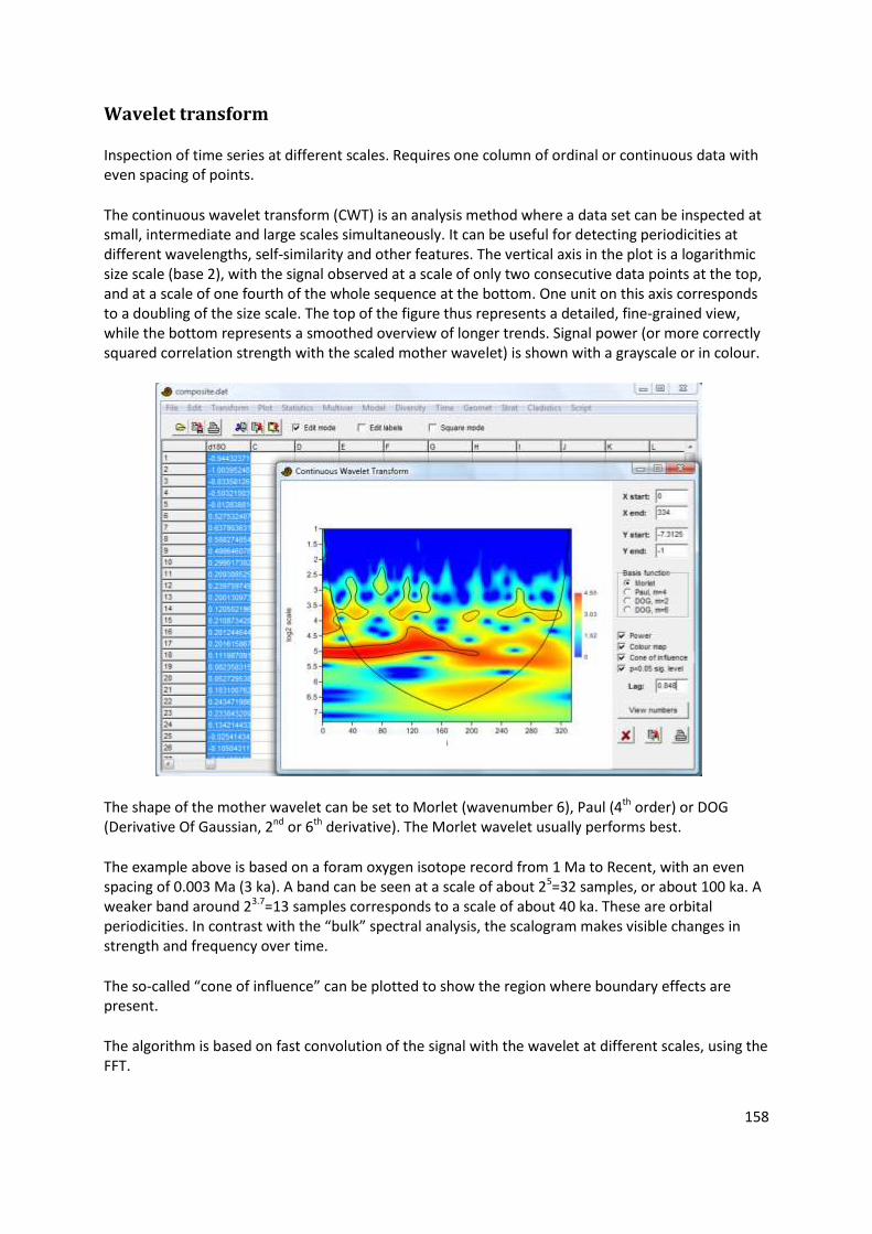
Wavelet transform
Inspection of time series at different scales. Requires one column of ordinal or continuous data with even spacing of points.
The continuous wavelet transform (CWT) is an analysis method where a data set can be inspected at small, intermediate and large scales simultaneously. It can be useful for detecting periodicities at different wavelengths, self-similarity and other features. The vertical axis in the plot is a logarithmic size scale (base 2), with the signal observed at a scale of only two consecutive data points at the top, and at a scale of one fourth of the whole sequence at the bottom. One unit on this axis corresponds to a doubling of the size scale. The top of the figure thus represents a detailed, fine-grained view, while the bottom represents a smoothed overview of longer trends. Signal power (or more correctly squared correlation strength with the scaled mother wavelet) is shown with a grayscale or in colour.
The shape of the mother wavelet can be set to Morlet (wavenumber 6), Paul (4th order) or DOG (Derivative Of Gaussian, 2nd or 6th derivative). The Morlet wavelet usually performs best.
The example above is based on a foram oxygen isotope record from 1 Ma to Recent, with an even spacing of 0.003 Ma (3 ka). A band can be seen at a scale of about 25=32 samples, or about 100 ka. A weaker band around 23.7=13 samples corresponds to a scale of about 40 ka. These are orbital periodicities. In contrast with the “bulk” spectral analysis, the scalogram makes visible changes in strength and frequency over time.
The so-called “cone of influence” can be plotted to show the region where boundary effects are present.
The algorithm is based on fast convolution of the signal with the wavelet at different scales, using the FFT.
159
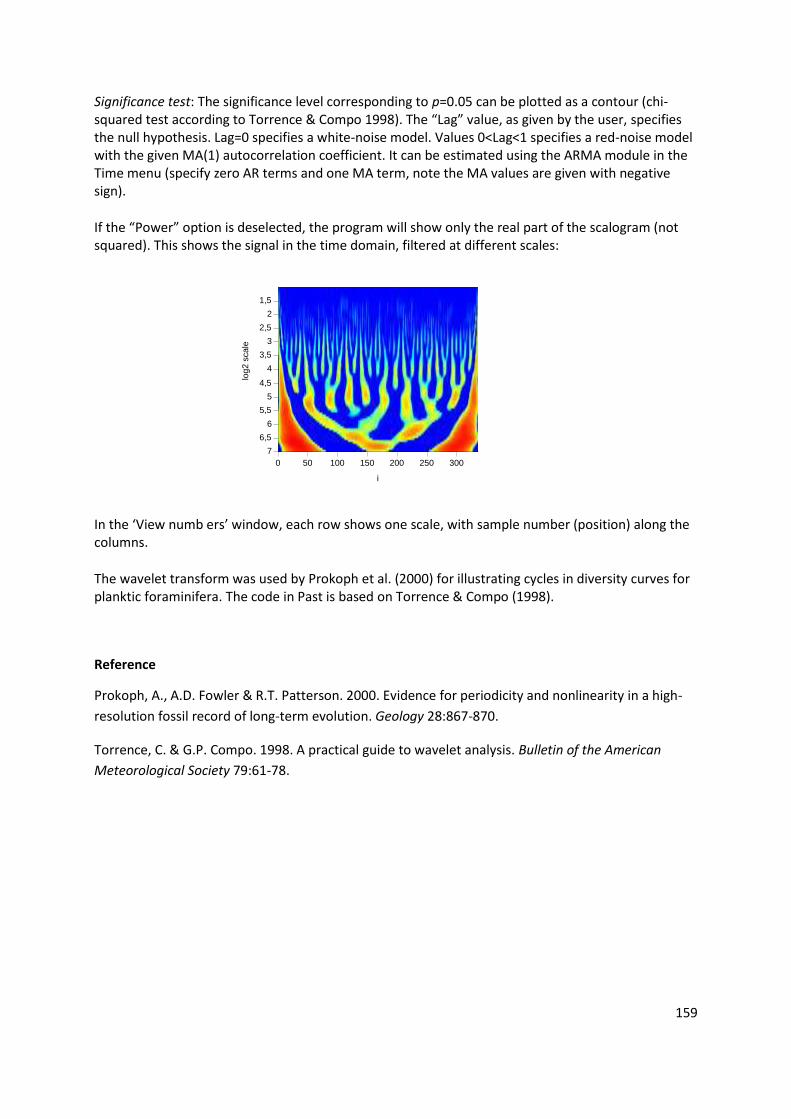
Significance test: The significance level corresponding to p=0.05 can be plotted as a contour (chi-squared test according to Torrence & Compo 1998). The “Lag” value, as given by the user, specifies the null hypothesis. Lag=0 specifies a white-noise model. Values 0<Lag<1 specifies a red-noise model with the given MA(1) autocorrelation coefficient. It can be estimated using the ARMA module in the Time menu (specify zero AR terms and one MA term, note the MA values are given with negative sign).
If the “Power” option is deselected, the program will show only the real part of the scalogram (not squared). This shows the signal in the time domain, filtered at different scales:
In the ‘View numb ers’ window, each row shows one scale, with sample number (position) along the columns.
The wavelet transform was used by Prokoph et al. (2000) for illustrating cycles in diversity curves for planktic foraminifera. The code in Past is based on Torrence & Compo (1998).
Reference
Prokoph, A., A.D. Fowler & R.T. Patterson. 2000. Evidence for periodicity and nonlinearity in a high-
resolution fossil record of long-term evolution. Geology 28:867-870.
Torrence, C. & G.P. Compo. 1998. A practical guide to wavelet analysis. Bulletin of the American
Meteorological Society 79:61-78.
0 50 100 150 200 250 300 i
7 6,5
6 5,5
5 4,5
4 3,5
3 2,5
2 1,5
log
2 s
cale
160
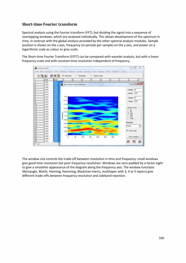
Short-time Fourier transform
Spectral analysis using the Fourier transform (FFT), but dividing the signal into a sequence of overlapping windows, which are analysed individually. This allows development of the spectrum in time, in contrast with the global analysis provided by the other spectral analysis modules. Sample position is shown on the x axis, frequency (in periods per sample) on the y axis, and power on a logarithmic scale as colour or grey scale.
The Short-time Fourier Transform (STFT) can be compared with wavelet analysis, but with a linear frequency scale and with constant time resolution independent of frequency.
The window size controls the trade-off between resolution in time and frequency; small windows give good time resolution but poor frequency resolution. Windows are zero-padded by a factor eight to give a smoother appearance of the diagram along the frequency axis. The window functions (Rectangle, Welch, Hanning, Hamming, Blackman-Harris, multitaper with 3, 4 or 5 tapers) give different trade-offs between frequency resolution and sideband rejection.
161
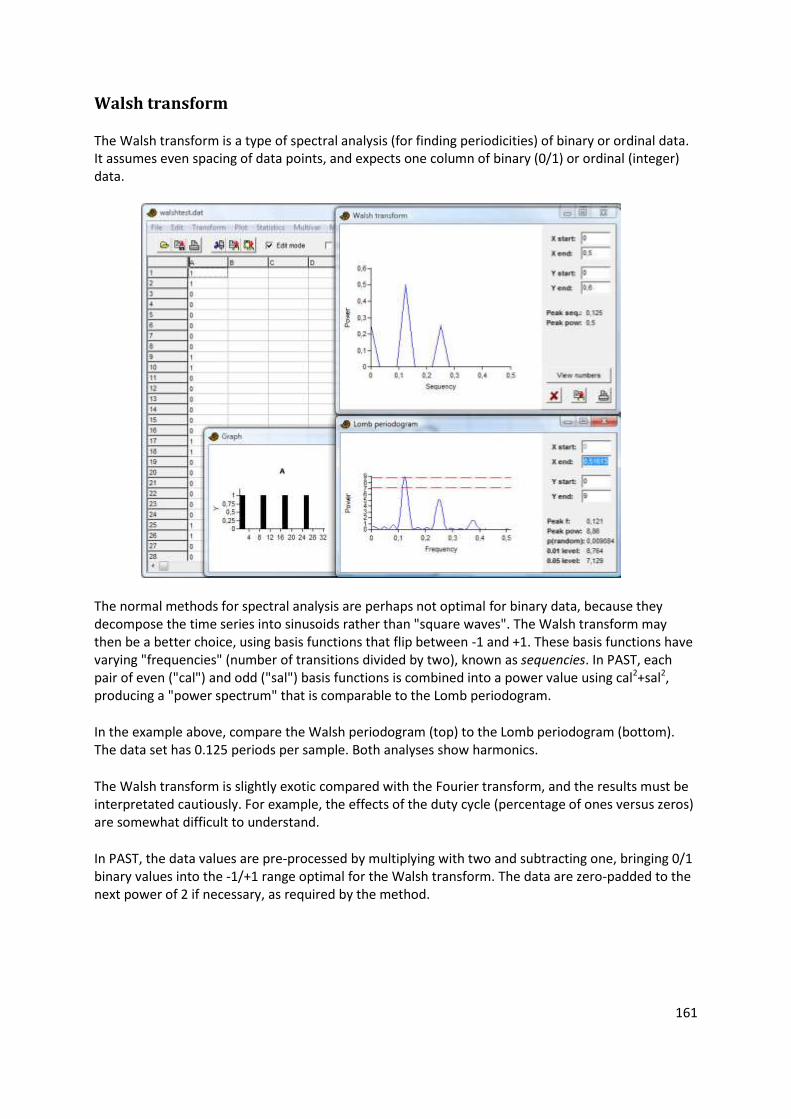
Walsh transform
The Walsh transform is a type of spectral analysis (for finding periodicities) of binary or ordinal data. It assumes even spacing of data points, and expects one column of binary (0/1) or ordinal (integer) data.
The normal methods for spectral analysis are perhaps not optimal for binary data, because they decompose the time series into sinusoids rather than "square waves". The Walsh transform may then be a better choice, using basis functions that flip between -1 and +1. These basis functions have varying "frequencies" (number of transitions divided by two), known as sequencies. In PAST, each pair of even ("cal") and odd ("sal") basis functions is combined into a power value using cal2+sal2, producing a "power spectrum" that is comparable to the Lomb periodogram.
In the example above, compare the Walsh periodogram (top) to the Lomb periodogram (bottom). The data set has 0.125 periods per sample. Both analyses show harmonics.
The Walsh transform is slightly exotic compared with the Fourier transform, and the results must be interpretated cautiously. For example, the effects of the duty cycle (percentage of ones versus zeros) are somewhat difficult to understand.
In PAST, the data values are pre-processed by multiplying with two and subtracting one, bringing 0/1 binary values into the -1/+1 range optimal for the Walsh transform. The data are zero-padded to the next power of 2 if necessary, as required by the method.
162
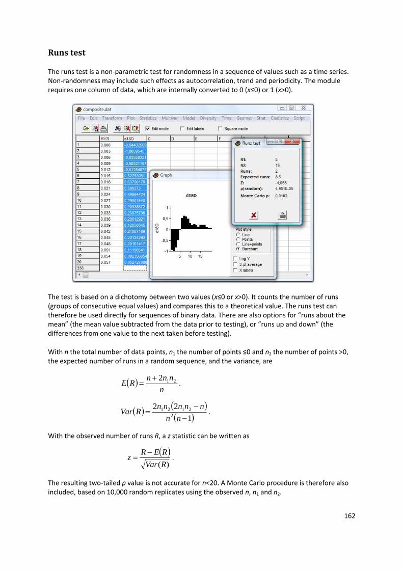
Runs test
The runs test is a non-parametric test for randomness in a sequence of values such as a time series. Non-randomness may include such effects as autocorrelation, trend and periodicity. The module requires one column of data, which are internally converted to 0 (x≤0) or 1 (x>0).
The test is based on a dichotomy between two values (x≤0 or x>0). It counts the number of runs (groups of consecutive equal values) and compares this to a theoretical value. The runs test can therefore be used directly for sequences of binary data. There are also options for “runs about the mean” (the mean value subtracted from the data prior to testing), or “runs up and down” (the differences from one value to the next taken before testing).
With n the total number of data points, n1 the number of points ≤0 and n2 the number of points >0, the expected number of runs in a random sequence, and the variance, are
n
nnnRE 212
.
122
2
2121
nn
nnnnnRVar .
With the observed number of runs R, a z statistic can be written as
)(RVar
RERz
.
The resulting two-tailed p value is not accurate for n<20. A Monte Carlo procedure is therefore also included, based on 10,000 random replicates using the observed n, n1 and n2.
163
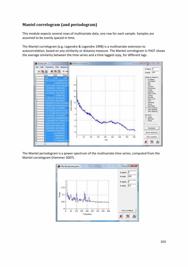
Mantel correlogram (and periodogram)
This module expects several rows of multivariate data, one row for each sample. Samples are assumed to be evenly spaced in time.
The Mantel correlogram (e.g. Legendre & Legendre 1998) is a multivariate extension to autocorrelation, based on any similarity or distance measure. The Mantel correlogram in PAST shows the average similarity between the time series and a time lagged copy, for different lags.
The Mantel periodogram is a power spectrum of the multivariate time series, computed from the Mantel correlogram (Hammer 2007).
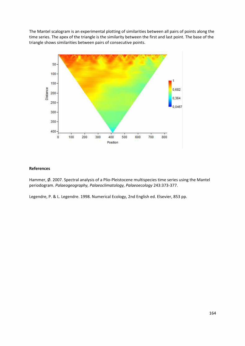
164
The Mantel scalogram is an experimental plotting of similarities between all pairs of points along the time series. The apex of the triangle is the similarity between the first and last point. The base of the triangle shows similarities between pairs of consecutive points.
References
Hammer, Ø. 2007. Spectral analysis of a Plio-Pleistocene multispecies time series using the Mantel periodogram. Palaeogeography, Palaeoclimatology, Palaeoecology 243:373-377.
Legendre, P. & L. Legendre. 1998. Numerical Ecology, 2nd English ed. Elsevier, 853 pp.
165
ARMA (and intervention analysis)
Analysis and removal of serial correlations in time series, and analysis of the impact of an external disturbance ("intervention") at a particular point in time. Stationary time series, except for a single intervention. One column of equally spaced data.
This powerful but somewhat complicated module implements maximum-likelihood ARMA analysis, and a minimal version of Box-Jenkins intervention analysis (e.g. for investigating how a climate change might impact biodiversity).
By default, a simple ARMA analysis without interventions is computed. The user selects the number of AR (autoregressive) and MA (moving-average) terms to include in the ARMA difference equation. The log-likelihood and Akaike information criterion are given. Select the numbers of terms that minimize the Akaike criterion, but be aware that AR terms are more "powerful" than MA terms. Two AR terms can model a periodicity, for example.
The main aim of ARMA analysis is to remove serial correlations, which otherwise cause problems for model fitting and statistics. The residual should be inspected for signs of autocorrelation, e.g. by copying the residual from the numerical output window back to the spreadsheet and using the autocorrelation module. Note that for many paleontological data sets with sparse data and confounding effects, proper ARMA analysis (and therefore intervention analysis) will be impossible.
The program is based on the likelihood algorithm of Melard (1984), combined with nonlinear multivariate optimization using simplex search.
Intervention analysis proceeds as follows. First, carry out ARMA analysis on only the samples preceding the intervention, by typing the last pre-intervention sample number in the "last samp" box. It is also possible to run the ARMA analysis only on the samples following the intervention, by typing the first post-intervention sample in the "first samp" box, but this is not recommended because of the post-intervention disturbance. Also tick the "Intervention" box to see the optimized intervention model.
The analysis follows Box and Tiao (1975) in assuming an "indicator function" u(i) that is either a unit step or a unit pulse, as selected by the user. The indicator function is transformed by an AR(1) process with a parameter delta, and then scaled by a magnitude (note that the magnitude given by PAST is the coefficient on the transformed indicator function: first do y(i)=delta*y(i-1)+u(i), then scale y by the magnitude). The algorithm is based on ARMA transformation of the complete sequence, then a corresponding ARMA transformation of y, and finally linear regression to find the magnitude. The parameter delta is optimized by exhaustive search over [0,1].
For small impacts in noisy data, delta may end up on a sub-optimum. Try both the step and pulse options, and see what gives smallest standard error on the magnitude. Also, inspect the "delta optimization" data, where standard error of the estimate is plotted as a function of delta, to see if the optimized value may be unstable.
The Box-Jenkins model can model changes that are abrupt and permanent (step function with delta=0, or pulse with delta=1), abrupt and non-permanent (pulse with delta<1), or gradual and permanent (step with delta<0).
166
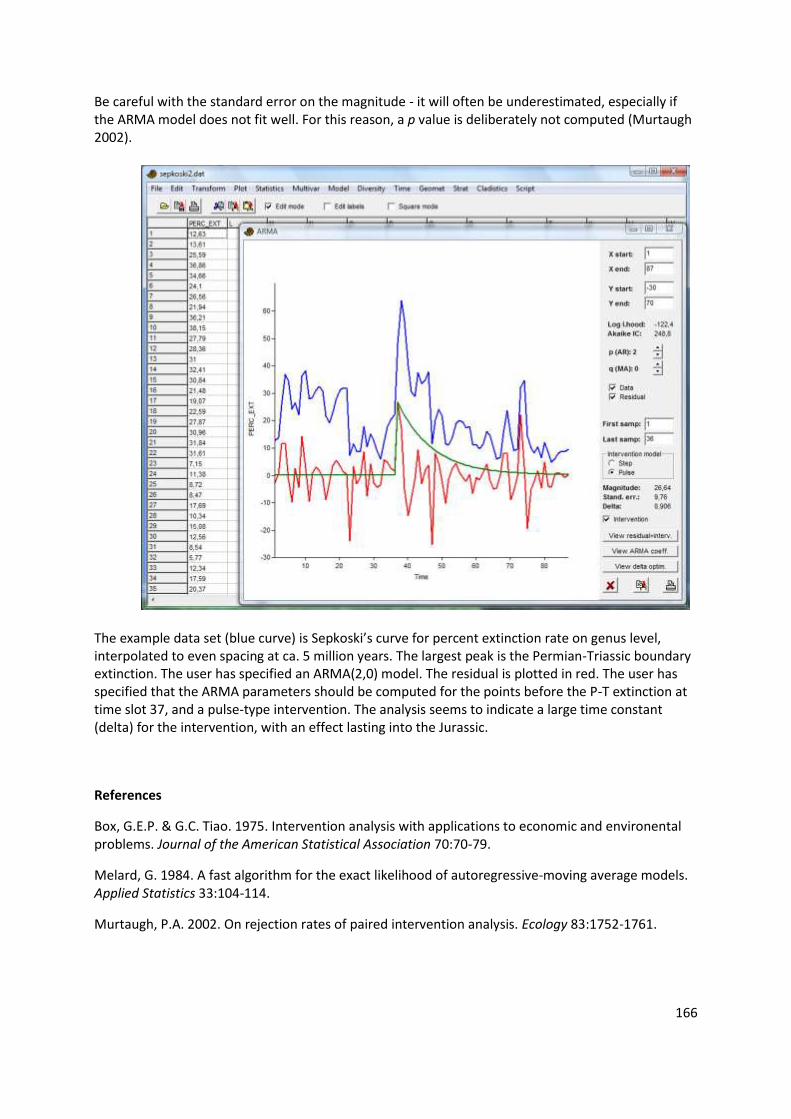
Be careful with the standard error on the magnitude - it will often be underestimated, especially if the ARMA model does not fit well. For this reason, a p value is deliberately not computed (Murtaugh 2002).
The example data set (blue curve) is Sepkoski’s curve for percent extinction rate on genus level, interpolated to even spacing at ca. 5 million years. The largest peak is the Permian-Triassic boundary extinction. The user has specified an ARMA(2,0) model. The residual is plotted in red. The user has specified that the ARMA parameters should be computed for the points before the P-T extinction at time slot 37, and a pulse-type intervention. The analysis seems to indicate a large time constant (delta) for the intervention, with an effect lasting into the Jurassic.
References
Box, G.E.P. & G.C. Tiao. 1975. Intervention analysis with applications to economic and environental problems. Journal of the American Statistical Association 70:70-79.
Melard, G. 1984. A fast algorithm for the exact likelihood of autoregressive-moving average models. Applied Statistics 33:104-114.
Murtaugh, P.A. 2002. On rejection rates of paired intervention analysis. Ecology 83:1752-1761.
167
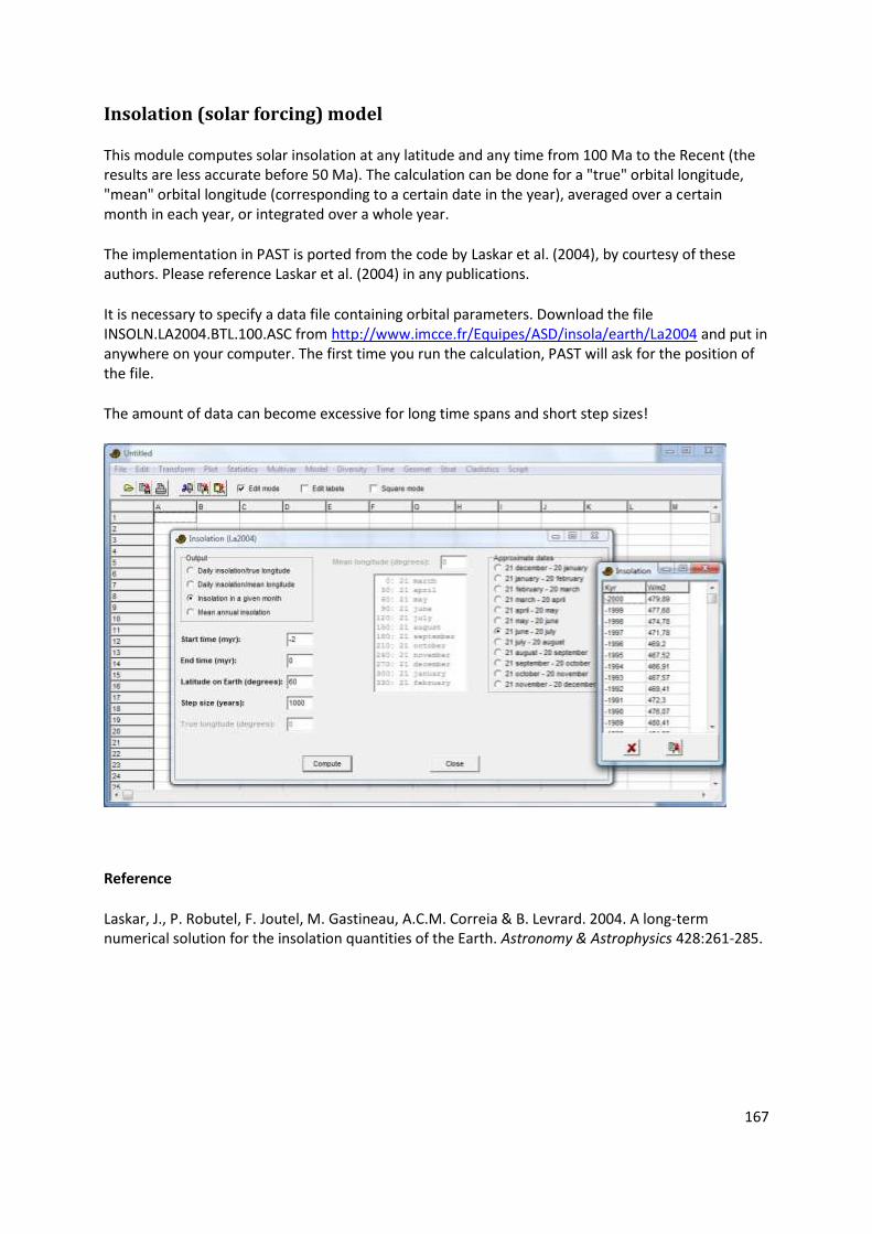
Insolation (solar forcing) model
This module computes solar insolation at any latitude and any time from 100 Ma to the Recent (the results are less accurate before 50 Ma). The calculation can be done for a "true" orbital longitude, "mean" orbital longitude (corresponding to a certain date in the year), averaged over a certain month in each year, or integrated over a whole year.
The implementation in PAST is ported from the code by Laskar et al. (2004), by courtesy of these authors. Please reference Laskar et al. (2004) in any publications.
It is necessary to specify a data file containing orbital parameters. Download the file INSOLN.LA2004.BTL.100.ASC from http://www.imcce.fr/Equipes/ASD/insola/earth/La2004 and put in anywhere on your computer. The first time you run the calculation, PAST will ask for the position of the file.
The amount of data can become excessive for long time spans and short step sizes!
Reference
Laskar, J., P. Robutel, F. Joutel, M. Gastineau, A.C.M. Correia & B. Levrard. 2004. A long-term numerical solution for the insolation quantities of the Earth. Astronomy & Astrophysics 428:261-285.
168
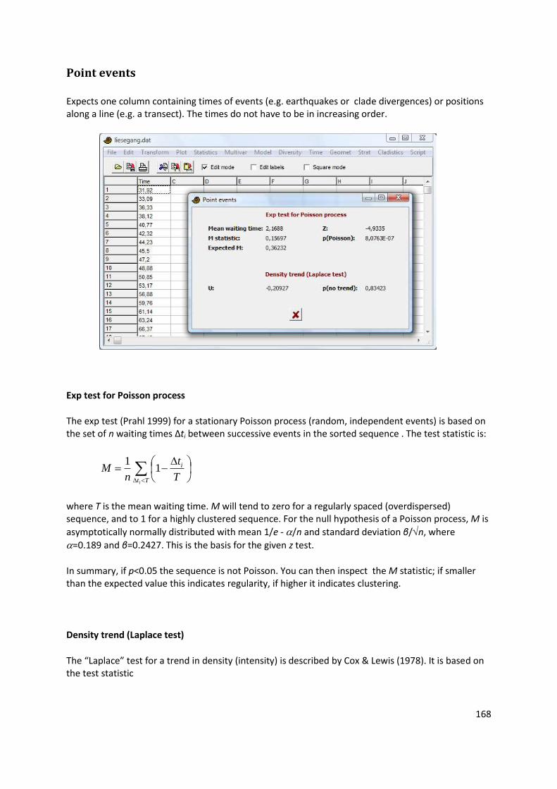
Point events
Expects one column containing times of events (e.g. earthquakes or clade divergences) or positions along a line (e.g. a transect). The times do not have to be in increasing order.
Exp test for Poisson process
The exp test (Prahl 1999) for a stationary Poisson process (random, independent events) is based on the set of n waiting times Δti between successive events in the sorted sequence . The test statistic is:
Tt
i
iT
t
nM 1
1
where T is the mean waiting time. M will tend to zero for a regularly spaced (overdispersed) sequence, and to 1 for a highly clustered sequence. For the null hypothesis of a Poisson process, M is
asymptotically normally distributed with mean 1/e - /n and standard deviation β/n, where
=0.189 and β=0.2427. This is the basis for the given z test.
In summary, if p<0.05 the sequence is not Poisson. You can then inspect the M statistic; if smaller than the expected value this indicates regularity, if higher it indicates clustering.
Density trend (Laplace test)
The “Laplace” test for a trend in density (intensity) is described by Cox & Lewis (1978). It is based on the test statistic
169
nL
Lt
U
12
1
2
where now t is the mean event time, n the number of events and L the length of the interval. L is estimated as the time from the first to the last event, plus the mean waiting time. U is approximately normally distributed with zero mean and unit variance under the null hypothesis of constant intensity. This is the basis for the given p value.
If p<0.05, a positive U indicates an increasing trend in intensity (decreasing waiting times), while a negative U indicates a decreasing trend. Note that if a trend is detected by this test, the sequence is not stationary and the assumptions of the exp test above are violated.
References
Cox, D. R. & P. A. W. Lewis. 1978. The Statistical Analysis of Series of Events. Chapman and Hall, London.
Prahl, J. 1999. A fast unbinned test on event clustering in Poisson processes. Arxiv, Astronomy and Astrophysics September 1999.
170
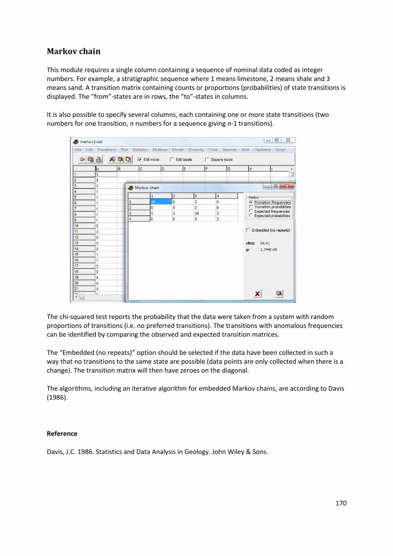
Markov chain
This module requires a single column containing a sequence of nominal data coded as integer numbers. For example, a stratigraphic sequence where 1 means limestone, 2 means shale and 3 means sand. A transition matrix containing counts or proportions (probabilities) of state transitions is displayed. The “from”-states are in rows, the “to”-states in columns.
It is also possible to specify several columns, each containing one or more state transitions (two numbers for one transition, n numbers for a sequence giving n-1 transitions).
The chi-squared test reports the probability that the data were taken from a system with random proportions of transitions (i.e. no preferred transitions). The transitions with anomalous frequencies can be identified by comparing the observed and expected transition matrices.
The “Embedded (no repeats)” option should be selected if the data have been collected in such a way that no transitions to the same state are possible (data points are only collected when there is a change). The transition matrix will then have zeroes on the diagonal.
The algorithms, including an iterative algorithm for embedded Markov chains, are according to Davis (1986).
Reference
Davis, J.C. 1986. Statistics and Data Analysis in Geology. John Wiley & Sons.
171
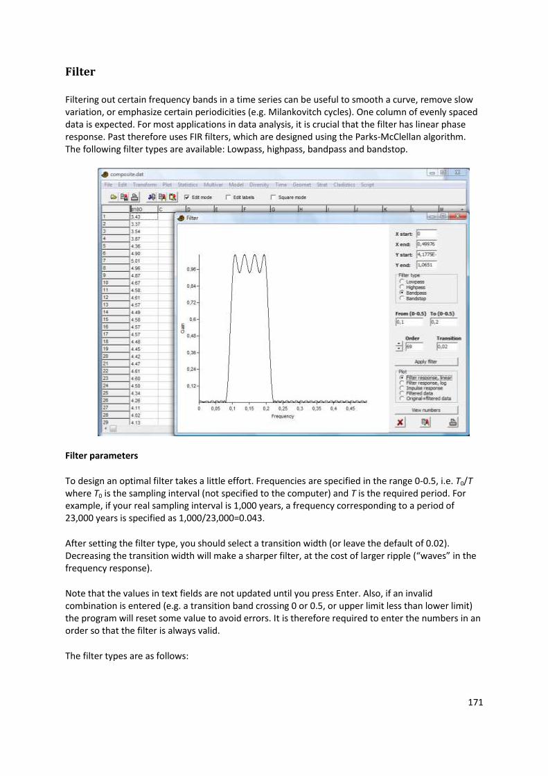
Filter
Filtering out certain frequency bands in a time series can be useful to smooth a curve, remove slow variation, or emphasize certain periodicities (e.g. Milankovitch cycles). One column of evenly spaced data is expected. For most applications in data analysis, it is crucial that the filter has linear phase response. Past therefore uses FIR filters, which are designed using the Parks-McClellan algorithm. The following filter types are available: Lowpass, highpass, bandpass and bandstop.
Filter parameters
To design an optimal filter takes a little effort. Frequencies are specified in the range 0-0.5, i.e. T0/T where T0 is the sampling interval (not specified to the computer) and T is the required period. For example, if your real sampling interval is 1,000 years, a frequency corresponding to a period of 23,000 years is specified as 1,000/23,000=0.043.
After setting the filter type, you should select a transition width (or leave the default of 0.02). Decreasing the transition width will make a sharper filter, at the cost of larger ripple (“waves” in the frequency response).
Note that the values in text fields are not updated until you press Enter. Also, if an invalid combination is entered (e.g. a transition band crossing 0 or 0.5, or upper limit less than lower limit) the program will reset some value to avoid errors. It is therefore required to enter the numbers in an order so that the filter is always valid.
The filter types are as follows:

172
1. Lowpass. The From frequency is forced to zero. Frequencies up to the To frequency pass the filter. Frequencies from To+Transition to 0.5 are blocked.
2. Highpass. The To frequency is forced to 0.5. Frequencies above the From frequency pass the filter. Frequencies from 0 to From-Transition are blocked.
3. Bandpass. Frequencies from From to To pass the filter. Frequencies below From-Transition and above To+Transition are blocked.
4. Bandstop. Frequencies from From to To are blocked. Frequencies from 0 to From-Transition and from To+Transition to 0.5 pass the filter.
Filter order
The filter order should be large enough to give an acceptably sharp filter with low ripple. However, a filter of length n will give less accurate results in the first and last n/2 samples of the the time series, which puts a practical limit on filter order for short series.
The Parks-McClellan algorithm will not always converge. This gives an obviously incorrect frequency response, and attempting to apply such a filter to the data will give a warning message. Try to change the filter order (usually increase it) to fix the problem.

173
Simple smoothers
A set of simple smoothers for a single column of evenly spaced data.
Missing data are supported.
Moving average
Simple n-point, centered moving average (n must be odd). Commonly used, but has unfortunate
properties such as a non-monotonic frequency response.
Gaussian
Weighted moving average using a Gaussian kernel with standard deviation set to 1/5 of the window
size (of n points). This is probably the best overall method in the module.
Moving median
Similar to moving average but takes the median instead of the mean. This method is more robust to
outliers.
AR 1 (exponential)
Recursive (autoregressive) filter, yi = yi-1 + (1-)xi with a smoothing coefficient from 0 to 1. This
corresponds to weighted averaging with exponentially decaying weights. Gives a phase delay and
also a transient in the beginning of the series. Included for completeness.
174
Date/time conversion
Utility to convert dates and/or times to a continuous time unit for analysis. The program expects one or two columns, each containing dates or times. If both are given, then time is added to date to give the final time value.
Dates can be given in the formats Year/Month/Day or Day/Month/Year. Years need all digits (a year given as 11 will mean 11 AD, not 2011). Only Gregorian calendar dates are supported. Leap years are taken into account.
Time can be given as Hours:Minutes or Hours:Minutes:Seconds (seconds can include decimals).
The output units can be years (using the Gregorian mean year of 365.2425 days), days (of 86400 seconds), hours, minutes or seconds.
The starting time (time zero) can be the smallest given time, the beginning of the first day, the beginning of the first year, year 0 (note the “astronomical” convention where the year before year 1 is year 0), or the beginning of the first Julian day (noon, year -4712).
The program operates with simple (UT) time, defined with respect to the Earth’s rotation and with a fixed number of seconds (86400) per day.
If your input data consists of space-separated date-time values, such as “2011/12/24 18:00:00.00”, then you may have to use the “Import text file” function to read the data such that dates and times are split into separate columns.
The calculation of Julian day (which is used to find number of days between two dates) follows Meeus (1991):
if month <= 2 begin year := year - 1; month := month + 12; end;
A = floor(year/100);
B = 2 – A + floor(A/4);
JD = floor(365.25(year + 4716)) + floor(30.6001(month+1)) + day + B – 1524.5;
Reference
Meeus, J. 1991. Astronomical algorithms. Willmann-Bell, Richmond.
175
Geometrical menu
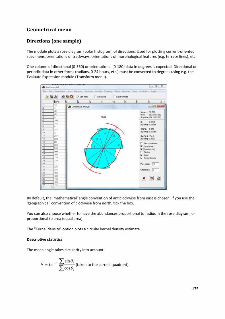
Directions (one sample) The module plots a rose diagram (polar histogram) of directions. Used for plotting current-oriented specimens, orientations of trackways, orientations of morphological features (e.g. terrace lines), etc. One column of directional (0-360) or orientational (0-180) data in degrees is expected. Directional or periodic data in other forms (radians, 0-24 hours, etc.) must be converted to degrees using e.g. the Evaluate Expression module (Transform menu).
By default, the 'mathematical' angle convention of anticlockwise from east is chosen. If you use the 'geographical' convention of clockwise from north, tick the box.
You can also choose whether to have the abundances proportional to radius in the rose diagram, or proportional to area (equal area).
The "Kernel density" option plots a circular kernel density estimate.
Descriptive statistics
The mean angle takes circularity into account:
i
i
cos
sintan 1 (taken to the correct quadrant).
176
The 95 percent confidence interval on the mean is estimated according to Fisher (1983). It assumes circular normal distribution, and is not accurate for very large variances (confidence interval larger than 45 degrees) or small sample sizes. The bootstrapped 95% confidence interval on the mean uses 5000 bootstrap replicates. The graphic uses the bootstrapped confidence interval.
The concentration parameter κ is estimated by iterative approximation to the solution to the equation
RI
I
0
1
where I0 and I1 are imaginary Bessel functions of orders 0 and 1, estimated according to Press et al. (1992), and R defined below (see e.g. Mardia 1972).
Rayleigh’s test for uniform distribution
The R value (mean resultant length) is given by:
nRn
i
i
n
i
i
2
1
2
1
sincos
.
R is further tested against a random distribution using Rayleigh's test for directional data (Davis 1986). Note that this procedure assumes evenly or unimodally (von Mises) distributed data - the test is not appropriate for e.g. bimodal data. The p values are computed using an approximation given by Mardia (1972):
2RnK
2
4322
288
97613224
4
21
n
KKKK
n
KKep K
Rao’s spacing test for uniform distribution
The Rao's spacing test (Batschelet 1981) for uniform distribution has test statistic
n
i
iTU12
1 ,
where no360 . iiiT 1 for i<n, 1
o360 nnT . This test is nonparametric, and
does not assume e.g. von Mises distribution. The p value is estimated by linear interpolation from the probability tables published by Russell & Levitin (1995).
A Chi-square test for uniform distribution is also available, with a user-defined number of bins (default 4).
177
The Watson’s U2 goodness-of-fit test for von Mises distribution
Let f be the von Mises distribution for estimated parameters of mean angle and concentration:
0
cos
2,;
I
ef
.
The test statistic (e.g. Lockhart & Stevens 1985) is
nzn
n
izU i
12
1
2
1
2
1222
2
where
dfzi
i 0,; ,
estimated by numerical integration. Critical values for the test statistic are obtained by linear interpolation into Table 1 of Lockhart & Stevens (1985). They are acceptably accurate for n>=20.
Axial data
The 'Orientations' option allows analysis of linear (axial) orientations (0-180 degrees). The Rayleigh and Watson tests are then carried out on doubled angles (this trick is described by Davis 1986); the Chi-square uses four bins from 0-180 degrees; the rose diagram mirrors the histogram around the origin.
References
Batschelet, E. 1981. Circular statistics in biology. Academic Press.
Davis, J.C. 1986. Statistics and Data Analysis in Geology. John Wiley & Sons.
Fisher, N.I. 1983. Comment on "A Method for Estimating the Standard Deviation of Wind Directions". Journal of Applied Meteorology 22:1971.
Lockhart, R.A. & M.A. Stephens 1985. Tests of fit for the von Mises distribution. Biometrika 72:647-652.
Mardia, K.V. 1972. Statistics of directional data. Academic Press, London.
Russell, G. S. & D.J. Levitin 1995. An expanded table of probability values for Rao's spacing test. Communications in Statistics: Simulation and Computation 24:879-888.
178
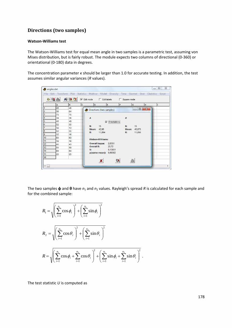
Directions (two samples)
Watson-Williams test
The Watson-Williams test for equal mean angle in two samples is a parametric test, assuming von Mises distribution, but is fairly robust. The module expects two columns of directional (0-360) or orientational (0-180) data in degrees.
The concentration parameter κ should be larger than 1.0 for accurate testing. In addition, the test assumes similar angular variances (R values).
The two samples φ and θ have n1 and n2 values. Rayleigh’s spread R is calculated for each sample and for the combined sample:
2
1
2
1
1
11
sincos
n
i
i
n
i
iR
2
1
2
1
2
22
sincos
n
i
i
n
i
iR
2
11
2
11
2121
sinsincoscos
n
i
i
n
i
i
n
i
i
n
i
iR .
The test statistic U is computed as
179
21
212RRn
RRRnU
.
The significance is computed by first correcting U according to Mardia (1972a):
95.08
31
45.01
81
2
2
nRU
nR
n
U
U
,
where n=n1+n2. The p value is then given by the F distribution with 1 and n-2 degrees of freedom. The combined concentration parameter κ is maximum-likelihood, computed as described under “Directions (one sample)” above.
Mardia-Watson-Wheeler test
This non-parametric test for equal distribution is computed according to Mardia (1972b).
2
2
2
2
2
1
2
1
2
12n
SC
n
SCW
where, for the first sample,
1
1
11 2cosn
i
i NrC ,
1
1
11 2sinn
i
i NrS
and similarly for the second sample (N=n1+n2). The r1i are the ranks of the values of the first sample within the pooled sample.
For N>14, W is approximately chi-squared with 2 degrees of freedom.
References
Mardia, K.V. 1972a. Statistics of directional data. Academic Press, London.
Mardia, K.V. 1972b. A multi-sample uniform scores test on a circle and its parametric competitor. Journal of the Royal Statistical Society Series B 34:102-113.
180
Circular correlations
Testing for correlation between two directional or orientational variates. Assumes “large” number of observations. Requires two columns of directional (0-360) or orientational (0-180) data in degrees.
This module uses the circular correlation procedure and parametric significance test of Jammalamadaka & Sengupta (2001).
The circular correlation coefficient r between vectors of angles α and β is
n
i
ii
n
i
ii
r
1
22
1
sinsin
sinsin
,
where the angular means are calculated as described previously. The test statistic T is computed as
n
k
kk
n
k
n
k
kk
rT
1
22
1 1
22
sinsin
sinsin
.
For large n, this statistic has asymptotically normal distribution with mean 0 and variance 1 under the null hypothesis of zero correlation, which is the basis for the calculation of p.
Reference
Jammalamadaka, S.R. & A. Sengupta. 2001. Topics in circular statistics. World Scientific.