Site-Specific Seismic Analyses Procedures for Framed ...cdn.intechopen.com/pdfs/27142/InTech-Site_specific... · In this chapter the procedure to carry out site-specific seismic analysis

7

Site-Specific Seismic Analyses Procedures for Framed Buildings for Scenario Earthquakes Including the Effect of Depth of Soil Stratum

P. Kamatchi1, G.V. Ramana2, A.K. Nagpal2 and Nagesh R. Iyer3 1Senior Scientist, CSIR-Structural Engineering Research Centre, Chennai

2Professor, Indian Institute of technology, Delhi 3Director, CSIR-Structural Engineering Research Centre, Chennai

India

1. Introduction

The importance of the effect of sediments above bedrock in modifying the strong ground

motion has been long recognized (Boore, 2004; Boore & Joyner, 1997; Idriss & Seed, 1970;

Seed & Idriss, 1969; Lam et al., 2001; Govindarajulu et al., 2004; Tezcan et al., 2002; Bakir et

al., 2005; Kamatchi et al., 2007) in literature. The nature of soil that changes the amplitude

and frequency content has a major influence on damaging effects of earthquake. To account

for these effects, most of the seismic codes, for example the Indian code (IS 1893 (Part 1)

2002) has defined response spectra for three types of soil viz., hard soil, medium soil and

soft soil. As an improvement over this approach, amplification factors based on empirical

and theoretical data (Borcherdt, 1994) have been introduced in International Building Codes

(IBC, 2009; ASCE 7 2005) for site classes A to E for the short period range and long period

range based on the average shear wave velocity of top 30 m soil stratum. For site class F (soft

soil) it has been recommended that site-specific analysis need to be carried out.

However, Sun et al. (2005) showed that the site coefficients specified in IBC 2000 (IBC 2000)

are not valid for Korean Peninsula due to the large difference in the depth of bedrock and

the soil stiffness profile. Further, building codes are highly simplified tools and do not

adequately represent any single earthquake event from a probable source for the site under

consideration. Recently, it is being suggested (Heuze et al., 2004 ) that in addition to use of

seismic code provisions, site-specific analysis which includes generation of strong ground

motion at bedrock level and propagating it through soil layers (Heuze et al., 2004; Mammo

2005; Balendra et al., 2002) and arriving at the design ground motions and response spectra

at surface should also be carried out.

In this chapter the procedure to carry out site-specific seismic analysis of framed buildings is

illustrated with examples for Delhi city. Rock outcrop motions are generated for the scenario

earthquakes of magnitude, Mw = 7.5, Mw = 8.0 and Mw = 8.5. Three actual soil sites of Delhi

have been modeled and the free field surface motions and the response spectra are obtained.

It has been observed that the PGA amplifications and the response spectra of the three sites

are quite different for the earthquakes considered. The same has reflected in considerable

www.intechopen.com

Earthquake Research and Analysis – New Frontiers in Seismology

196

difference in base shear and displacement response of reinforced concrete (RC) framed

buildings when assumed to be located on the chosen three sites.

Major revisions are taking place in seismic codes towards performance based design (ATC

40 1996; FEMA 273&274, 1996). Response spectra which forms the basis for the demand

curve in performance based design is of interest to many structural engineers. Having

understood the importance of site-specific analysis, in this chapter, procedure for carrying

out performance evaluation of buildings for site-specific earthquakes accounting for

different depths of soil stratum is illustrated with an example.

Further, addressing to the complexity involved in carrying out site-specific seismic analysis,

as an alternative, artificial neural network (ANN) based methodology is proposed in this

chapter. The steps involved in the development of ANN models for site-specific seismic

analysis viz., the process of identification of input and output parameters by carrying out

sensitivity analysis, identification of suitable architecture and training of ANN, checking the

performance of ANN and validating the performance of ANN with examples are illustrated

in this chapter for Delhi city.

2. Steps involved in site-specific seismic analysis for scenario earthquake

Major steps involved in site-specific seismic analysis are identification of scenario

earthquake, generation of strong ground motion for a rock site, propagation of ground

motion through soil stratum and to arrive at the surface level response spectrum.

2.1 Identification of scenario earthquake When this study was carried out (Kamatchi, 2008), not much of information was available

on earthquake catalogue for Delhi capital city of India. Hence the scenario earthquakes have

been chosen deterministically as per the information available from literature. Seismologists

(Bilham et al., 1998; Singh et al., 2002) have reported that three major thrust planes viz.,

Main Central Thrust (MCT), Main Boundary Thrust (MBT) and Main Frontal Thrust (MFT)

exist in Himalayas due to the relative movement of Indian plate by 5 cm/year with respect

to Eurasian plate. Khattri (1999) has estimated the probability of occurrence of a great

earthquake of moment magnitude 8.5 from the large unbroken segment called central

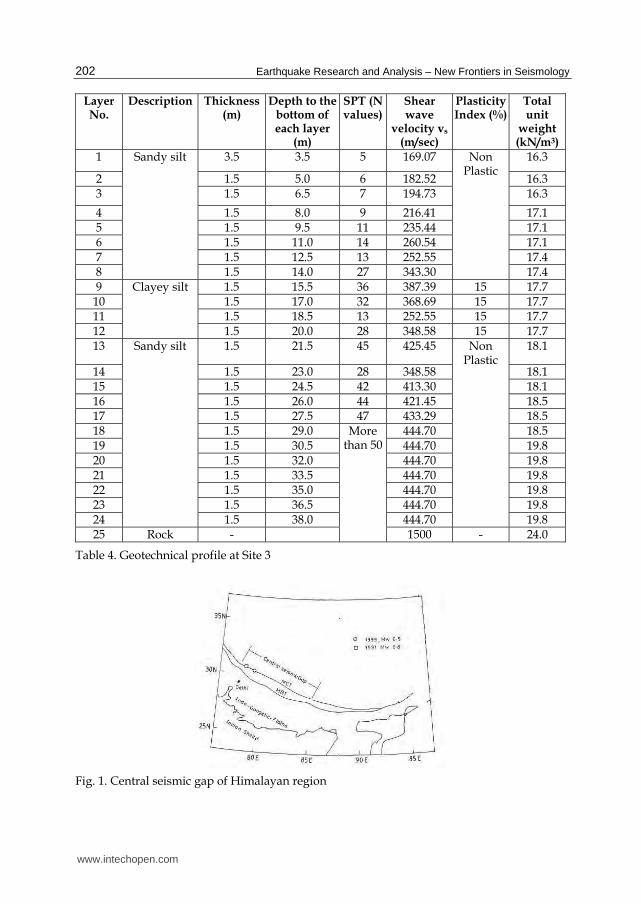
seismic gap (Fig. 1) between MBT and MCT in the next 100 years to be 0.59. Delhi is situated

at a distance of roughly 200 km from MBT and 300 km from MCT. Hence in the present

study scenario earthquakes for Delhi city are assumed to be originated from central seismic

gap of Himalayan region.

2.2 Generation of strong ground motion Generation of artificial strong motions using stochastic models by identifying major fault zones and propagating seismic waves generated at these potential sources to the sites of interest is well accepted in literature (Boore 1983&2003; Beresnev & Atkinson 2002). In this process, path effects and anelastic attenuation effects predicted by the empirical and theoretical models (Beresnev & Atkinson 2002 ) are used. For source representation, point source models (Boore & Atkinson 1987) or finite source models (Hartzell, 1978) are widely used. Stochastic simulation procedure for ground motion generation based on seismological models using point source model has been proposed by Boore (1983&2003). In this

www.intechopen.com


197

procedure the band limited Gaussian white noise is windowed and filtered in the time domain and transformed into frequency domain. The Fourier amplitude spectrum is scaled to the mean squared absolute spectra and multiplied by a Fourier amplitude spectrum obtained from source path effects. Then, the spectrum is transformed back to time domain and the time history is obtained. From the analysis of recorded ground motions, it has been reported (Beresnev & Atkinson

1997) that point source models are not capable of reproducing the characteristic features of

large earthquakes (Mw > 6) viz., long duration and radiation of less energy at low to

intermediate frequencies (0.2-2 Hz). Simulation of strong ground motion from finite fault

model has been developed by Beresnev and Atkinson (1997&1998). In this model, the fault

rupture plane is represented with an array of sub-faults and the radiation from each sub-

fault is modeled as a point source similar to Boore’s model (Boore, 1983). According to finite

source model, the fault rupture initiates at the hypocenter and spreads uniformly along the

fault plane radially outward with a constant rupture velocity triggering radiation from sub-

faults in succession. The improvements to finite source model viz., extended finite source

model (Motazedian & Atkinson, 2005) implementing the effects of radiated energy on sub-

fault size and dynamic corner frequency, are reported in literature when this chapter is

written, however finite sources model (Beresnev & Atkinson 1997&1998) is used in the

studies reported in this chapter. The details of the Fourier amplitude spectrum adopted in

the present study and the assumptions made are illustrated subsequently.

The Fourier amplitude spectrum A() of the point source of one element (sub-fault) is

defined (Boore, 1983; Boore & Atkinson 1987; Brune, 1970) as

2( ) ( ) ( ) ( ) ( )nA S P G R A (1)

Where, is the angular frequency, S() is the source function, P() is the filter function for

high frequency attenuation, G(R) is the geometric attenuation function, An() is anelastic

whole path attenuation function. S(), P(), G(R) and An() are further defined below:

2.2.1 Source function, S()

The shape and amplitude of the theoretical source spectrum (2-model, Aki (1967) is given

by,

32

1( )

41 /

o

c

PFR mS w

R (2)

where, P is the partition factor to represent one horizontal component, F is the free surface

amplification factor, R is the spectral average for radiation pattern, mo is the seismic

moment of a sub-fault, c is the corner frequency, is the density in the vicinity of the

source in g/cm3, is the shear wave velocity in km/sec and R is the epicentral distance in

km. In the simulation of ground motion for Delhi region in the present study, the values of

different parameters are adopted (Singh et al., 2002) as P=1/2.0; F=2.0; R = 0.55; =2.85

gm/cc and = 3.6 km/sec.

The moment magnitude (Mw) which defines the size of earthquake is related (Hanks &

Kanamori 1979) to seismic moment (Mo) of the earthquake by,

www.intechopen.com


198

0.67 log 10.7w oM M (3)

The rupture area (A) and sub-fault length (l) corresponding to a moment magnitude of earthquake can be calculated from empirical equations (Beresnev & Atkinson, 1998) as follows,

log 4.0wA M (4)

log 2 0.4 wl M (5)

For a sub-fault of equal dimensions (w=l, w, l being the dimensions of the sub-fault) the seismic moment of a sub-fault, mo is given by

3om l (6)

where Δσ is the stress parameter (Beresnev & Atkinson, 1998). The number of sub sources (Nsub) to be summed to reach the target seismic moment (Mo) is given by

osub

o

MN

m (7)

The corner frequency c governs the acceleration amplitude and controls the frequency content of the earthquake at source is given by,

2 r sc

y z

l (8)

where, yr is the constant representing the ratio of rupture velocity to shear wave velocity of source which is set to a value of 0.8 by Beresnev and Atkinson (1997), zs is the parameter indicating maximum rate of slip also known as strength factor. The value of zs may vary from 0.5 to 2.0 and in the present study a value of 1.4 (Singh et al., 2002) has been adopted for the simulation of earthquake motions for Delhi region.

2.2.2 Filter function for high frequency attenuation, P() In order to account for the high frequency attenuation by the near-surface weathered layer

either a fourth order Butterworth filter with cut off frequency m =2fmax or a spectral decay

parameter kappa () is widely used in stochastic models. In the present study, Butter worth

filter function P() with cutoff frequency fmax = 15 Hz (Singh et al., 2002) has been adopted.

1/2

8( ) 1 / mP (9)

2.2.3 Geometric attenuation factor, G(R) Geometric attenuation accounts for the decay and type of seismic waves. According to Singh et al. (2002) and Herrmann and Kijko (1983) for a distance of twice the crustal thickness the body waves dominate (direct seismic shear waves) and after that surface waves dominate (reflected Lg waves). Depending on the earth’s crust thickness tri-linear or bilinear relationships are used for the calculation of G. The thickness of crust near Delhi

www.intechopen.com


199

has been reported to be 45 - 50 km (Tewari & Kumar, 2003) and bilinear relationship (Eq. 10) is adopted in the present study.

1( )G R

R R<100 km (10a)

1( )

100G R

R R>100 km (10b)

2.2.4 Anelastic whole path attenuation factor, An()

The anelastic whole path attenuation factor An() which represents wave energy loss due to

radiation damping of rock is accounted by this factor An (),

2( )

RQ

nA e (11)

where Q is the quality factor. The Q factor depends on the wave transmission quality of

rock. For Himalayan arc region Q factor has been estimated by Singh et al. (2002) from the

available earthquake records as follows.

0.48( ) 508Q f f

(12)

where, f is the frequency in Hz.

2.2.5 Simulation of time history The Fourier amplitude spectrum derived from the section above gives the frequency content

of the earthquake ground motion. This frequency information is combined with random

phase angles in a stochastic process to generate artificial ground motion (Boore, 1983) for

each sub-fault. Simulations from each sub-fault are lagged and summed to get the time

history of earthquake.

Duration of the sub-fault time window, Tw is represented as the sum of its source duration,

Ts and distance dependant duration, Td (Beresnev & Atkinson, 1997; Boore 2003).

w s dT T T (13)

In references Beresnev and Atkinson (1997) and Boore (2003), Ts is taken as proportional to

inverse of the corner frequency (1/fc) and Td is taken as 0.05R.

Finite fault simulation program (FINSIM) has been widely used for the generation of

ground motions of large size earthquakes (Atkinson & Beresnev, 2002; Beresnev & Atkinson

1998; Roumelioti & Beresnev 2003; Singh et al., 2002) and hence has been adopted in the

present study.

The seismological parameters (Table 1) used in the generation of rock outcrop motions for Delhi region have been broadly adopted from Singh et al. (2002). In order to minimize the noise due to random fault rupture in the simulation, 15 ground motions have been generated for each earthquake magnitude. One of the simulations of the time histories generated for rock outcrop (Ridge observatory) in the present study have been compared (Fig. 2), with one simulation obtained from Singh (2005), for each of the magnitudes 7.5, 8.0, 8.5.

www.intechopen.com


200

Parameters Mw = 7.5 Mw = 8.0 Mw = 8.5

Fault orientation Strike 300 Dip 7 Strike 300 Dip 7 Strike 300 Dip 7 Fault dimension along strike and dip (km)

56 by 56 125 by 80 240 by 80

Depth of focus (km) 11 16 16

Stress parameter (bars) 50 50 50

No. of sub-faults 5x5 8x5 16x5

No. of sub-sources summed

28 57 339

Duration Model 1/fc +0.05R 1/fc +0.05R 1/fc +0.05R

Quality factor 508f0.48 508f0.48 508f0.48

Windowing function Saragoni-Hart Saragoni-Hart Saragoni-Hart

fmax (Hz) 15 15 15

Crustal shear wave velocity (km/sec)

3.6 3.6 3.6

Crustal density (kN/m3)

2.8 2.8 2.8

Radiation strength factor

1.4 1.4 1.4

Table 1. Seismological parameters for strong motion generation

3. Propagation of strong ground motion through soil layer using one dimensional equivalent linear analysis

One dimensional equivalent linear vertical wave propagation analysis is the widely used

numerical procedure for modeling soil amplification problem (Idriss, 1990; Yoshida et al.,

2002). In one dimensional wave propagation analysis, soil deposit is assumed to be having

number of horizontal layers with different shear modulus (G), damping () and unit weight

(). In the linear analysis, G and are assumed to be constant in each layer. Since the soil

will be subjected to nonlinear strain (Yoshida et al., 2002) even under small earthquake

excitation equivalent linear analysis is preferred over linear analysis and the equivalent

linear analysis program SHAKE (Ordonez, 2000, Schnabel et al., 1972 ) is used in the present

study. Equivalent linear modulus reduction (G/Gmax) and damping ratio () curves generated

from laboratory test results are adopted from Vucetic and Dobry (1991) depending on the

plasticity index of different soil layers. Since SHAKE is a total stress analysis program

(Schnabel et al., 1972) depth of water table has not been considered in the analysis.

3.1 Typical soil strata for Delhi region Three actual soil sites designated as site 1, site 2 and site 3 located in Delhi as shown in Fig. 3

are chosen in the present study. The layer wise soil characteristics (medium type) and the

depth to the base of the layer from the surface is given in Tables 2 to 4. The shear wave

velocity, Vs measurements are not available for the sites chosen. However the variations of

N values with depth are available from the geotechnical data as given in Tables 2 to 4. The

variation of shear wave velocity along the depth in the present study is obtained by using

the correlations suggested for Delhi region by Rao and Ramana (2004) as given in eq. 14.

www.intechopen.com


201

Vs =79 N 0.43 (sand) (14a)

Vs =86 N 0.42 (silty sand/sandy silt) (14b)

Layer No.

Description Thickness (m)

Depth to the bottom of each layer

(m)

SPT (N values)

Shear wave velocity vs

(m/sec)

Plasticity Index (%)

Total unit

weight (kN/m3)

1 Sandy silt of low

plasticity

3.5 3.5 13 252.55 7

16.3 2 1.5 5 17 282.67

3 1.5 6.5 20 302.64

4 1.5 8 23 320.94

5 Sandy silt of low

Plasticity

1.5 9.5 28 348.58 7

16.9 6 1.5 11 32 368.69

7 1.5 12.5 35 382.83

8 1.5 14 37 391.87 6

18.1

9 1.5 15.5 42 413.30 18.5

10 1.5 17 47 433.29 18.5

11 Rock - - 1500 - 24.0

Table 2. Geotechnical profile at Site 1

Layer No.



(m)

SPT (N values)

Shear wave

velocity vs (m/sec)


Total unit

weight (kN/m3)

1 Clayey silt of low plasticity

1.5 1.5 9 216.41 11 16.9

2 1.5 3.0 9 216.41 15 17.4

3 Sandy silt 1.5 4.5 12 229.97 Non Plastic

17.4

4 Fine sand 1.5 6.0 12 229.97 17.2

5 1.5 7.5 12 229.97 17.1

6 1.5 9.0 13 238.03 17.1

7 1.5 10.5 15 253.13 17.1

8 1.5 12.0 19 280.21 17.1

9 1.5 13.5 20 286.46 17.7

10 1.5 15.0 21 292.54 17.7

11 1.5 16.5 26 320.68 17.7

12 Sandy silt of low plasticity

1.5 18.0 31 363.81 17.7

13 1.5 19.5 41 409.14 17.7

14 1.5 21.0 41 409.14 6 19.8

15 1.5 22.5 41 409.14 19.8

16 Rock - - 1500 - 24.0


www.intechopen.com


202

Layer No.



(m)

SPT (N values)

Shear wave

velocity vs (m/sec)


Total unit

weight (kN/m3)

1 Sandy silt 3.5 3.5 5 169.07 Non Plastic

16.3

2 1.5 5.0 6 182.52 16.3 3 1.5 6.5 7 194.73 16.3

4 1.5 8.0 9 216.41 17.1 5 1.5 9.5 11 235.44 17.1 6 1.5 11.0 14 260.54 17.1 7 1.5 12.5 13 252.55 17.4 8 1.5 14.0 27 343.30 17.4 9 Clayey silt 1.5 15.5 36 387.39 15 17.7 10 1.5 17.0 32 368.69 15 17.7 11 1.5 18.5 13 252.55 15 17.7 12 1.5 20.0 28 348.58 15 17.7 13 Sandy silt 1.5 21.5 45 425.45 Non

Plastic 18.1

14 1.5 23.0 28 348.58 18.1 15 1.5 24.5 42 413.30 18.1 16 1.5 26.0 44 421.45 18.5 17 1.5 27.5 47 433.29 18.5 18 1.5 29.0 More

than 50444.70 18.5

19 1.5 30.5 444.70 19.8 20 1.5 32.0 444.70 19.8 21 1.5 33.5 444.70 19.8 22 1.5 35.0 444.70 19.8 23 1.5 36.5 444.70 19.8 24 1.5 38.0 444.70 19.8 25 Rock - 1500 - 24.0


Fig. 1. Central seismic gap of Himalayan region

www.intechopen.com


203

(a) Mw = 7.5 (b)Mw = 8.0

(c) Mw =8.5

Fig. 2. Comparison of artificial ground motions generated for a rock site at Delhi for earthquakes from central seismic gap with similar generations from literature

Fig. 3. Location of three soil sites of Delhi region

www.intechopen.com


204

4. Response of three sites for the scenario earthquakes

The amplification ratios and response spectra are the engineering outputs required to

calculate the response of buildings for site-specific analysis. Shear wave velocity of bedrock

(quartzite) at Delhi is reported to be in the range of 1000 m/s to 2000 m/s (Parvez et al.,

2004). The rock outcrop motions simulated as per the procedure given in section 2.2 are

considered as bedrock motions for soil sites and the same are propagated through the soil

strata of the three sites and the free field motions are obtained. As a typical case the bedrock

level and free field motions at the top of three sites for one simulation of earthquake (Mw =

7.5) for the three magnitudes are shown in Fig. 4.

The variations of average amplification ratios of 15 earthquake simulations for the three sites

are obtained. As a typical case, variations of average amplification ratios for Mw = 8.5

earthquake is shown in Fig. 5 for the three earthquake magnitudes. It can be seen from the

results that the peak amplification ratios as well as the frequencies at which the peak

amplification ratios occur are quite different for the three sites. The fundamental time

periods of the three sites for different earthquakes are given in Table 5. Difference in site

period for larger magnitude earthquake is due to nonlinear response of soil sites for higher

magnitudes.

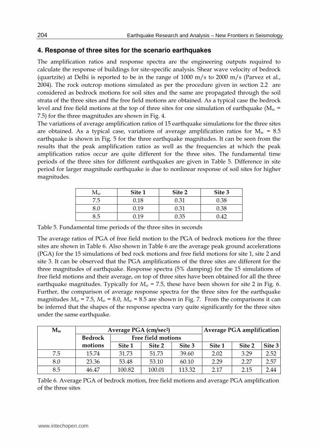
Mw Site 1 Site 2 Site 3

7.5 0.18 0.31 0.38

8.0 0.19 0.31 0.38

8.5 0.19 0.35 0.42

Table 5. Fundamental time periods of the three sites in seconds

The average ratios of PGA of free field motion to the PGA of bedrock motions for the three

sites are shown in Table 6. Also shown in Table 6 are the average peak ground accelerations

(PGA) for the 15 simulations of bed rock motions and free field motions for site 1, site 2 and

site 3. It can be observed that the PGA amplifications of the three sites are different for the

three magnitudes of earthquake. Response spectra (5% damping) for the 15 simulations of

free field motions and their average, on top of three sites have been obtained for all the three

earthquake magnitudes. Typically for Mw = 7.5, these have been shown for site 2 in Fig. 6.

Further, the comparison of average response spectra for the three sites for the earthquake

magnitudes Mw = 7.5, Mw = 8.0, Mw = 8.5 are shown in Fig. 7. From the comparisons it can

be inferred that the shapes of the response spectra vary quite significantly for the three sites

under the same earthquake.

Mw Average PGA (cm/sec2) Average PGA amplification

Bedrock

motions

Free field motions

Site 1 Site 2 Site 3 Site 1 Site 2 Site 3

7.5 15.74 31.73 51.73 39.60 2.02 3.29 2.52

8.0 23.36 53.48 53.10 60.10 2.29 2.27 2.57

8.5 46.47 100.82 100.01 113.32 2.17 2.15 2.44

Table 6. Average PGA of bedrock motion, free field motions and average PGA amplification of the three sites

www.intechopen.com


205

Fig. 4. Bedrock level and free field motions at the top of three sites for one simulation of earthquake, Mw =7.5

Fig. 5. Variations of average amplification ratios for the three sites, Mw = 8.5

Fig. 6. Response spectra (5% damping) for the 15 simulations of free field motions and their average, Mw =7.5; Site 2

www.intechopen.com


206

(a) Mw = 7.5 (b) Mw = 8.0

(c) Mw = 8.5

Fig. 7. Comparison of average response spectra for the three sites

5. Response of buildings on the three sites

It is clearly seen from the comparison of response spectra, that buildings situated on the

three sites will be subjected to different force levels during the same earthquake. In order to

demonstrate the site-specific response of buildings, a three storey building and a fifteen

storey building designated as B1 and B2 with plan details as shown in Fig. 8 are chosen for

the present study. The buildings are assumed to be situated on the three soil sites (Fig. 3)

chosen at Delhi. The earthquake is applied in y direction. Both the buildings are assumed to

be having frames as stiffening elements with uniform beam and column sections along the

height of the building. The beams are assumed to be axially rigid and have infinite flexural

rigidity. All the columns are square and are assumed to be axially rigid. The structural

properties of buildings are given in Table 7. The storey shears have been obtained by

response spectrum method as per IS 1893(Part 1)-2002, (2002). In the evaluation of storey

shears response reduction factor has been taken equal to one.

www.intechopen.com


207

Building Moment of inertia of square columns 10-4 (m4)

Storey height (m)

No. of stories

Mass of all the floors except

top floor (kN-sec2/m)

Mass of the top

floor (kN-sec2/m)

B1 11.1 (Frames 1,8)

21.0 (Frames 2,3,4,5,6,7)

3.0 3 410 205

B2 108.0 (Frames 1,4)

108.0 (Frames 2,3)

3.5 15 500 300

Table 7. Structural properties of the buildings

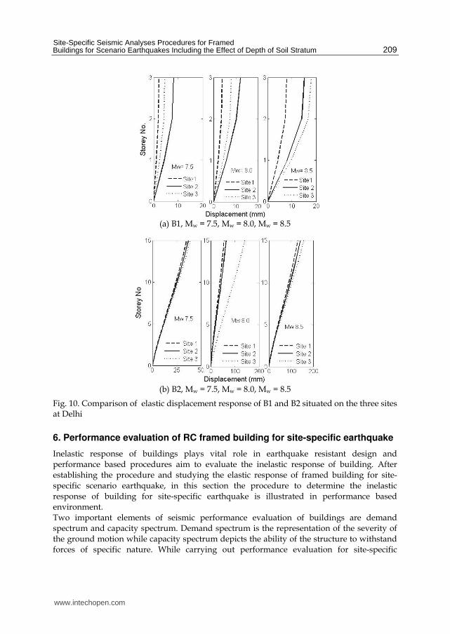
The comparison of storey shears for buildings B1 and B2 for site-specific earthquakes and storey shears obtained by considering the three sites as medium soil sites(MS) for design basis earthquake(DBE) as per seismic code IS 1893 (Part 1)-2002, (2002) for Delhi are shown in Fig. 9. For both the buildings storey shears obtained as per IS 1893 (Part 1)-2002, (2002) are different from the storey shears from site-specific analysis. Comparison of displacement responses for B1 and B2 are given in Fig. 10. It may be noted that, larger variation in base shear and displacement response for different sites for B1 is observed due to the proximity of fundamental time period (0.3 sec) of B1 to the site periods (Table 5).

Fig. 8. Plan of buildings B1, B2

www.intechopen.com


208

(a) B1, Mw = 7.5 (b) B1, Mw = 8.0

(c) B1, Mw = 8.5 (d) B2, Mw = 7.5

(e) B2, Mw = 8.0 (f) B2, Mw = 8.5

Fig. 9. Comparison of elastic storey shear of B1 and B2 situated on three sites at Delhi

www.intechopen.com


209

(a) B1, Mw = 7.5, Mw = 8.0, Mw = 8.5

(b) B2, Mw = 7.5, Mw = 8.0, Mw = 8.5

Fig. 10. Comparison of elastic displacement response of B1 and B2 situated on the three sites at Delhi

6. Performance evaluation of RC framed building for site-specific earthquake

Inelastic response of buildings plays vital role in earthquake resistant design and performance based procedures aim to evaluate the inelastic response of building. After establishing the procedure and studying the elastic response of framed building for site-

specific scenario earthquake, in this section the procedure to determine the inelastic response of building for site-specific earthquake is illustrated in performance based environment.

Two important elements of seismic performance evaluation of buildings are demand spectrum and capacity spectrum. Demand spectrum is the representation of the severity of the ground motion while capacity spectrum depicts the ability of the structure to withstand forces of specific nature. While carrying out performance evaluation for site-specific

www.intechopen.com


210

earthquake, code based response spectrum needs to be replaced with site-specific spectrum and the same will be considered as demand spectrum. Capacity spectrum method (ATC 40, 1996; FEMA 273&274, 1996) has provisions to modify a demand spectrum to account for

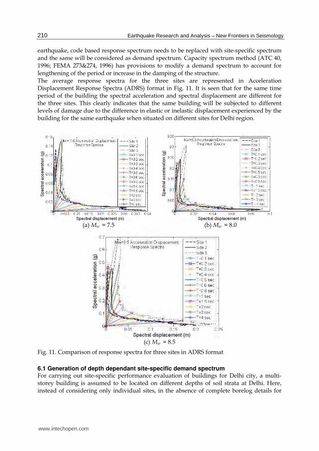
lengthening of the period or increase in the damping of the structure. The average response spectra for the three sites are represented in Acceleration Displacement Response Spectra (ADRS) format in Fig. 11. It is seen that for the same time period of the building the spectral acceleration and spectral displacement are different for the three sites. This clearly indicates that the same building will be subjected to different levels of damage due to the difference in elastic or inelastic displacement experienced by the building for the same earthquake when situated on different sites for Delhi region.

(a) Mw = 7.5 (b) Mw = 8.0

(c) Mw = 8.5

Fig. 11. Comparison of response spectra for three sites in ADRS format

6.1 Generation of depth dependant site-specific demand spectrum For carrying out site-specific performance evaluation of buildings for Delhi city, a multi-storey building is assumed to be located on different depths of soil strata at Delhi. Here, instead of considering only individual sites, in the absence of complete borelog details for

www.intechopen.com


211

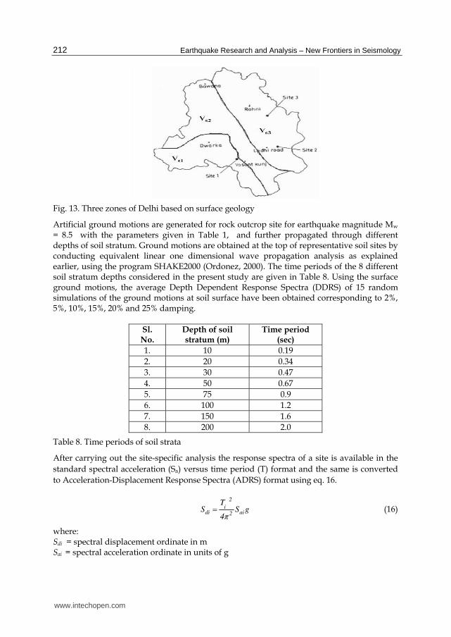
greater depths, representative soil sites of different depths are considered. The thickness of alluvium above the bedrock at Delhi varies significantly and according to a report by Central Ground Water Board (CGWB) (2002), variation is from less than 50 m to more than 300 m (Fig. 12). In the present study 8 representative soil strata defined by depths 10m, 20m, 30m, 50m, 75m, 100m, 150m and 200m have been chosen. Shear wave velocity, modulus reduction curve and damping curve are the other important properties that influence the modification of ground motion through soil layer. For shear wave velocity, regression relations (Eq. 15) have been suggested by Satyam (2006) based on seismic refraction and MASW tests. Based on the measured values, Delhi has been divided into three regions (Fig. 13) viz., (i) south and south central Delhi, (ii) north and north western Delhi and (iii) trans Yamuna Delhi. Separate shear wave velocity models viz., Vs1, Vs2, Vs3 has been proposed for each region as given in equation 15.

Vs1 =281 Ds 0.08 (South and South Central Delhi) (15a)

Vs2 =217 Ds 0.13 (West and North Western Delhi) (15b)

Vs3 =140 Ds 0.24 (Trans Yamuna, Delhi) (15c)

where Ds is the depth of soil stratum below the ground level in m. However, the model Vs3 only has been considered for the performance evaluation of building in the present study. For dynamic characteristics, from the large number of borelog data available for Delhi region, it is observed that the Plasticity Index (PI) of soils at Delhi region varies from 0% to 15%. Modulus reduction curves and damping curves for Delhi soil corresponding to PI=0% (Non plastic), PI=15% (low plasticity) soil have been adopted as explained in section 3 from Vucetic and Dobry (1991). For rock, modulus reduction curves and damping curves have been chosen from Schnabel and Seed (1972).

Fig. 12. Thickness of alluvium above bedrock (CGWB, 2002)

www.intechopen.com


212

Fig. 13. Three zones of Delhi based on surface geology

Artificial ground motions are generated for rock outcrop site for earthquake magnitude Mw = 8.5 with the parameters given in Table 1, and further propagated through different depths of soil stratum. Ground motions are obtained at the top of representative soil sites by conducting equivalent linear one dimensional wave propagation analysis as explained earlier, using the program SHAKE2000 (Ordonez, 2000). The time periods of the 8 different soil stratum depths considered in the present study are given in Table 8. Using the surface ground motions, the average Depth Dependent Response Spectra (DDRS) of 15 random simulations of the ground motions at soil surface have been obtained corresponding to 2%, 5%, 10%, 15%, 20% and 25% damping.

Sl. No.

Depth of soil stratum (m)

Time period (sec)

1. 10 0.19

2. 20 0.34

3. 30 0.47

4. 50 0.67

5. 75 0.9

6. 100 1.2

7. 150 1.6

8. 200 2.0

Table 8. Time periods of soil strata

After carrying out the site-specific analysis the response spectra of a site is available in the

standard spectral acceleration (Sa) versus time period (T) format and the same is converted

to Acceleration-Displacement Response Spectra (ADRS) format using eq. 16.

2

idi ai2

TS S g

4π (16)

where: Sdi = spectral displacement ordinate in m Sai = spectral acceleration ordinate in units of g

www.intechopen.com


213

Ti = time period of the building in secs g = acceleration due to gravity in m/s2 i = ith point of the spectra

6.2 Generation of capacity spectrum from capacity curve through nonlinear static analysis Plan of an eight storey building chosen (designated as B3) for the present study is shown in

Fig. 14. Overall length and width of the building are 11.4m and 10.9m, respectively. Height

of the building is 23.6m. Cross section and reinforcement details of the beams and columns

are modeled as given in the construction drawings of the building. The total lumped mass

due to dead and participating live loads of the building for the bottom six stories is equal to

179.2 tons while the lumped mass for seventh and eighth stories is equal to 90.1 tons and

17.9 tons, respectively. Building is modeled using SAP2000 computer program (2004), with

default PMM hinge properties for column and default M3 properties for beam.

Displacement controlled nonlinear static pushover analysis has been carried out for the 3D

building model and the capacity curve of the building is obtained. Further, the capacity

curve is transformed to capacity spectrum using Eqns. 17 and 18.

j

aj

1

V

WSα

(17)

roof

dj

1 1,roof

ΔS

PF .φ (18)

where:

Vj = base shear at the jth point of the capacity curve

W = weight of the building as sum of dead load and percentage live load

┙1 = modal mass coefficient for the first natural mode

Δroof = roof displacement

PF1 = modal participation factor for the first natural mode

1,roof = amplitude at roof level in first natural mode

6.3 Determination of performance point In the present study, site-specific demand spectrum for 2%, 5%, 10%, 15%, 20% and 25%

damping are obtained for the building. According to ATC 40 (1996), effective damping

(βeff) of the building during earthquake excitation is combination of viscous damping that

is inherent in the building (about 5%) and hysteretic damping (┚o) (that is related to the

area inside the hysteretic loops formed when the earthquake force is plotted against the

structural displacement). In view of this, it is required to modify the demand spectrum to

account for the effective damping of the structure. An iterative method as suggested by

authors (Kamatchi et al., 2010a) is used to determine the performance point, wherein,

demand spectrum has to be updated in each iterative cycle till convergence is achieved. In

the process, effective damping is obtained as per the procedure suggested in ATC 40

(1996).

www.intechopen.com


214

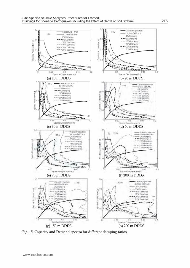
6.3.1 Performance points for the chosen building The capacity and demand curves for the eight different depths of soil stratum are obtained

for building and shown in Fig. 15. For the soil stratum depths of 10m, 20m, 30m, 50m and

200m, the 5% demand curve intersect the capacity curve in the elastic response region. For

the other depths (75m, 100m and 150m), the intersection points are found to lie in inelastic

response region. For these three depths, spectral reduction factors are applied to 5% demand

spectra and the performance points are obtained as per ATC 40 (1996). This is carried out

through number of trials as shown in Fig. 16. The trial performance points are arrived by

using effective damping (┚eff), Spectral reduction factor for acceleration predominant region

(SRA) and velocity predominant region (SRv) corresponding to soil stratum depths of 75m,

100m and 150m. The base shear (Vb) and roof displacements(inel) corresponding to the final

performance points of the building for 75m, 100m and 150m depths of soil stratum are

compared with corresponding values obtained for DBE earthquake and Medium soil site

conditions as per IS 1893(Part 1)-2002 (2002) in Table 9.

Depth of

soil

stratum

(m)

Vb (kN) Δinel (m)

Site-specific DBE %

difference

Site-

specific

DBE %

difference

75 1235.91 928.56 33.10 0.071 0.049 44.90

100 1381.7 928.56 48.80 0.093 0.049 89.80

150 1338.05 928.56 44.10 0.077 0.049 57.14

Table 9. Comparison of Vb and Δinel for reduced spectra with DBE

Fig. 14. Plan of the building, B3

www.intechopen.com


215

(a) 10 m DDDS (b) 20 m DDDS

(c) 30 m DDDS (d) 50 m DDDS

(e) 75 m DDDS (f) 100 m DDDS

(g) 150 m DDDS (h) 200 m DDDS

Fig. 15. Capacity and Demand spectra for different damping ratios

www.intechopen.com


216

(a) 75 m DDDS (b) 100 m DDDS

(c) 150 m DDDS

Fig. 16. Performance points using ATC 40 (1996) procedure for different soil stratum depths, DDDS and IS 1893(Part 1)-2002 medium soil demand spectra

7. Development of artificial neural networks for site-specific seismic analysis of buildings

In the earlier sections, procedure for carrying out site-specific analysis for scenario

earthquakes is demonstrated with examples of RC framed buildings. It is accepted in

literature, site-specific seismic analysis is mandatory for sites of specific soil (F type) (IBC

2009) and for earthquake-resistant design of important and critical structures. It is being

insisted in this chapter that, even for other structures, and for medium soil, it is preferred to

carry out a detailed site-specific analysis to arrive at the design force levels. Site-specific

analysis requires considerable modelling and computational effort w.r.t. representing the

generation as well as propagation of strong ground motion and it’s effect on the structures.

As an alternative, ANN models are generated in this chapter for the prediction of site-

specific spectral accelerations.

Standard feed forward back propagation neural network algorithm with one hidden layer

has been adopted to implement this. The main advantage of the neural network model lies

in calculation of the realistic site-specific design base shear values without the need to

generate strong ground motions and complex modelling of the soil profile.

www.intechopen.com


217

7.1 Input and output parameters for ANN models

Initially the following parameters are identified as probable input parameters and the

average spectral acceleration (Sa/g) is identified as the output parameter for sensitivity

analysis.

Moment magnitude of the earthquake (Mw),

Shear wave velocity of rock half-space (Vsr),

Average plasticity index of the soil stratum (PI),

Average soil density of the soil stratum (), Depth of the soil stratum above the bedrock (h),

Shear wave velocity model (Vsm),

Damping ratio of SDOF oscillator () and

Time period of the SDOF oscillator (Tb)

Based on the results of the sensitivity studies (Kamatchi, 2008; Kamatchi et al., 2010b) for the

development of neural network models five input parameters viz., Mw, h, , Tb, Vsm and one

output parameter Sa/g are chosen.

7.2 Choosing the configuration of the neural networks

Multilayer neural network with neurons in all the layers and fully connected in a feed

forward manner has been chosen for the present implementation. Sigmoid function (with

output in the range of 0 to 1) is used for activation and the back propagation learning

algorithm is used for training. The feed forward back propagation algorithm has been used

successfully for many civil engineering applications and is considered as one of the most

efficient algorithms for engineering applications (Adeli, 2001). One hidden layer has been

chosen for the network and the number of neurons in the hidden layer is decided in the

learning process by trial and error.

7.3 Training of neural network

As the number of data sets is large, for the sake of convenience in handling the data during

training, it has been decided to have two neural networks. The soil stratum depths up to 75

m have been taken in the first network designated as NET1 with rest of the parameters

assuming all the values in their respective ranges. Similarly, the second network designated

as NET2 includes soil stratum depths up to 200 m and has number of patterns as that for

NET1, i.e., 49815. The data has been randomly partitioned (Reich & Barai, 1999), with two

third of the data sets being used for training and the remaining are used for testing. The

number of sampling points for the input parameters and the number of data sets are shown

in Table 10.

Input parameter Number of data sets

Mw Vsm h(m) Tb ( sec) Total Training Testing

3 3 3 15 123 49815 35000 14815

Table 10. Number of sampling points for the input parameters and number of data sets for

NET1 and NET2

www.intechopen.com


218

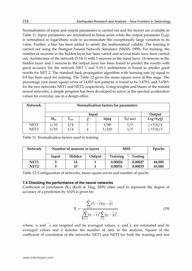
Normalisation of input and output parameters is carried out and the factors are available in

Table 11. Input parameters are normalised in linear sense while the output parameter (Sa/g)

is normalised in logarithmic scale to accommodate the exceptionally large variation in its

value. Further, a bias has been added to satisfy the mathematical validity. The training is

carried out using the Stuttgart Neural Network Simulator (SNNS, 1999). For training, the

number of neurons in the hidden layer has been varied and several trials have been carried

out. Architecture of the network (5-14-1) with 5 neurons in the input layer, 14 neurons in the

hidden layer and 1 neuron in the output layer has been found to predict the results with

good accuracy for the network NET 1 and 5-15-1 architecture is found to predict good

results for NET 2. The standard back propagation algorithm with learning rate () equal to

0.9 has been used for training. The Table 12 gives the mean square error at this stage. The

percentage root mean square error of 14,815 test patterns is found to be 3.479% and 3.658%

for the two networks NET1 and NET2, respectively. Using weights and biases of the trained

neural networks, a simple program has been developed to arrive at the spectral acceleration

values for everyday use in a design office.

Network Normalization factors for parameters

Input Output

Mw Vsm h(m) Tb( sec) Log (Sa/g)

NET1 NET2

1/10 1/10

1/4 1/4

7 4

1/80 1/210

1/5 1/5

( +3.5)/4 ( +3.0)/3

Table 11. Normalization factors used in training

Network Number of neurons in layers MSE Epochs

Input Hidden Output Training Testing

NET1 NET2

5 5

14 15

1 1

0.00024 0.00031

0.00027 0.00033

44,000 65,000

Table 12. Configuration of networks, mean square errors and number of epochs

7.4 Checking the performance of the neural networks Coefficient of correlation (Rc) (Kerh & Ting, 2005) often used to represent the degree of

accuracy of a prediction by ANN is given by:

1

2 2

1 1

( )( )

( ) ( )

n

i ii

cn n

i ii i

x x y y

R

x x y y

(19)

where, xi and x are targeted and its averaged values, yi andy are estimated and its

averaged values and n denotes the number of data in the analysis. Square of the

coefficient of correlation of the networks NET1 and NET2 for both the training and test

www.intechopen.com


219

patterns are found to be more than 0.9 which guarantees better performance of network

for any new input.

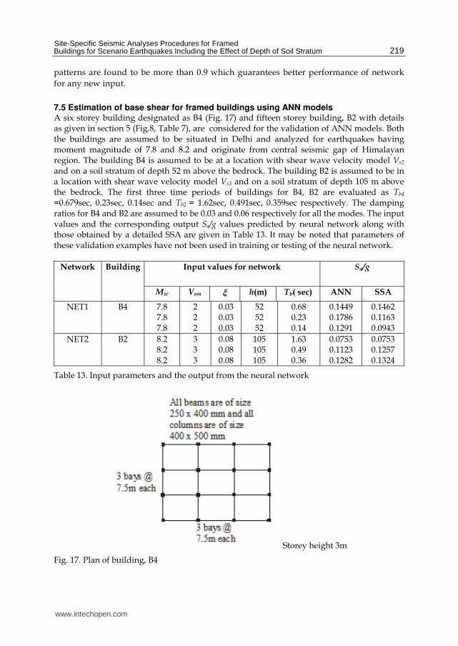
7.5 Estimation of base shear for framed buildings using ANN models A six storey building designated as B4 (Fig. 17) and fifteen storey building, B2 with details as given in section 5 (Fig.8, Table 7), are considered for the validation of ANN models. Both the buildings are assumed to be situated in Delhi and analyzed for earthquakes having moment magnitude of 7.8 and 8.2 and originate from central seismic gap of Himalayan region. The building B4 is assumed to be at a location with shear wave velocity model Vs2 and on a soil stratum of depth 52 m above the bedrock. The building B2 is assumed to be in a location with shear wave velocity model Vs3 and on a soil stratum of depth 105 m above the bedrock. The first three time periods of buildings for B4, B2 are evaluated as Tb4

=0.679sec, 0.23sec, 0.14sec and Tb2 = 1.62sec, 0.491sec, 0.359sec respectively. The damping ratios for B4 and B2 are assumed to be 0.03 and 0.06 respectively for all the modes. The input values and the corresponding output Sa/g values predicted by neural network along with those obtained by a detailed SSA are given in Table 13. It may be noted that parameters of these validation examples have not been used in training or testing of the neural network.

Network Building Input values for network Sa/g

Mw Vsm h(m) Tb( sec) ANN SSA

NET1 B4 7.8 7.8 7.8

2 2 2

0.03 0.03 0.03

52 52 52

0.68 0.23 0.14

0.1449 0.1786 0.1291

0.1462 0.1163 0.0943

NET2 B2 8.2 8.2 8.2

3 3 3

0.08 0.08 0.08

105 105 105

1.63 0.49 0.36

0.0753 0.1123 0.1282

0.0753 0.1257 0.1324

Table 13. Input parameters and the output from the neural network

Storey height 3m

Fig. 17. Plan of building, B4

www.intechopen.com


220

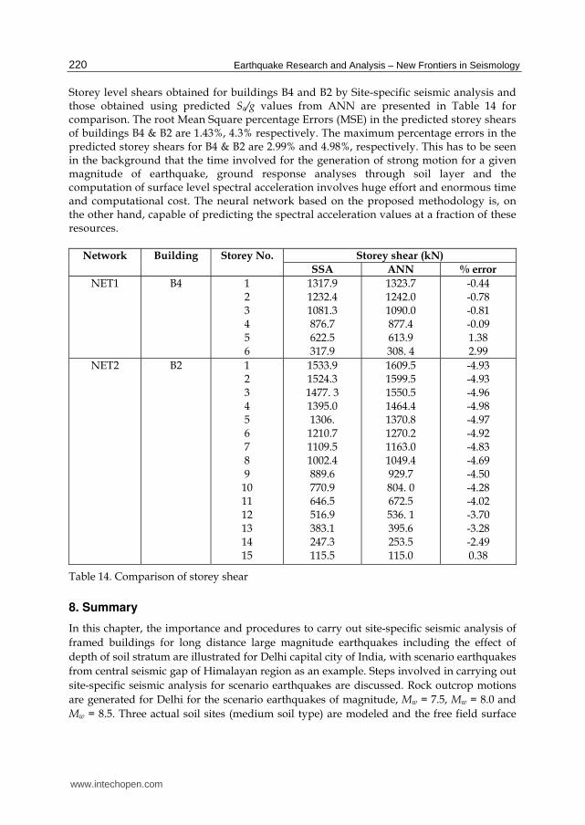
Storey level shears obtained for buildings B4 and B2 by Site-specific seismic analysis and those obtained using predicted Sa/g values from ANN are presented in Table 14 for comparison. The root Mean Square percentage Errors (MSE) in the predicted storey shears of buildings B4 & B2 are 1.43%, 4.3% respectively. The maximum percentage errors in the predicted storey shears for B4 & B2 are 2.99% and 4.98%, respectively. This has to be seen in the background that the time involved for the generation of strong motion for a given magnitude of earthquake, ground response analyses through soil layer and the computation of surface level spectral acceleration involves huge effort and enormous time and computational cost. The neural network based on the proposed methodology is, on the other hand, capable of predicting the spectral acceleration values at a fraction of these resources.

Network Building Storey No. Storey shear (kN)

SSA ANN % error

NET1 B4 1 2 3 4 5 6

1317.9 1232.4 1081.3 876.7 622.5 317.9

1323.7 1242.0 1090.0 877.4 613.9 308. 4

-0.44 -0.78 -0.81 -0.09 1.38 2.99

NET2 B2 1 2 3 4 5 6 7 8 9

10 11 12 13 14 15

1533.9 1524.3 1477. 3 1395.0 1306.

1210.7 1109.5 1002.4 889.6 770.9 646.5 516.9 383.1 247.3 115.5

1609.5 1599.5 1550.5 1464.4 1370.8 1270.2 1163.0 1049.4 929.7 804. 0 672.5 536. 1 395.6 253.5 115.0

-4.93 -4.93 -4.96 -4.98 -4.97 -4.92 -4.83 -4.69 -4.50 -4.28 -4.02 -3.70 -3.28 -2.49 0.38

Table 14. Comparison of storey shear

8. Summary

In this chapter, the importance and procedures to carry out site-specific seismic analysis of

framed buildings for long distance large magnitude earthquakes including the effect of

depth of soil stratum are illustrated for Delhi capital city of India, with scenario earthquakes

from central seismic gap of Himalayan region as an example. Steps involved in carrying out

site-specific seismic analysis for scenario earthquakes are discussed. Rock outcrop motions

are generated for Delhi for the scenario earthquakes of magnitude, Mw = 7.5, Mw = 8.0 and

Mw = 8.5. Three actual soil sites (medium soil type) are modeled and the free field surface

www.intechopen.com


221

motions and the response spectra are obtained. It has been observed that the PGA

amplifications and the response spectra of the three sites are quite different for the

earthquakes considered. It is clear from response of two RC framed building that the

performance of the buildings will be different when situated on three different soil sites.

From the studies made, it can be concluded that, it may be necessary to perform the site-

specific analyses of buildings at sites having medium types of soil as well.

Having established the importance of carrying out site-specific seismic analysis for

moderate sites and RC framed buildings, the procedure to carry out seismic performance

evaluation of existing building for site-specific earthquake is demonstrated for an eight

storey building assumed to be situated on different depths of soil stratum for Delhi region.

Rock outcrop motions generated for earthquake of Mw = 8.5 are propagated through

different depths of representative soil stratum and depth dependant demand spectrum are

obtained. The effect of depth dependant response spectrum on the performance of building

is studied for eight different depths of soil stratum above bedrock. From the studies made,

it is clear that considering the design spectra suggested by seismic codes and only the top 30

m soil stratum to include the effects of soil amplification may not ensure safe seismic

performance of a building. It is further seen that the site-specific earthquake and the depth

of soil stratum have significant influence on the performance of the building both in terms of

inelastic displacement as well as inelastic base shear.

Procedure to develop ANN models to rapidly estimate the site-specific spectral acceleration

of structures is illustrated with Delhi as an example. From the results of sensitivity studies

conducted earlier for Delhi city, moment magnitude of the earthquake, Mw, depth of the soil

stratum above the bedrock, h, shear wave velocity model, Vsm, damping ratio, and time

period, Tb, of the SDOF oscillator are identified as governing input parameters for

predicting the output of spectral acceleration, Sa/g.

Excellent performance of the trained neural networks has been demonstrated by the

calculated values of coefficient of correlation. Trained neural networks are validated by

using borelog data of an actual soil site. In addition, the neural networks have been

validated for two different buildings assumed to be located in Delhi city. Performance of

ANN models developed are checked and validated with number of examples. Validation

results for two different buildings included in this chapter indicates that the root mean

square percentage error is within tolerable values for both the buildings analysed in the

present study.

The procedures suggested in this chapter is suitable for carrying out site-specific seismic

analysis for framed buildings for any region for which information about seismic hazard in

terms of scenario earthquake and the relevant geological and geotechnical details of the

region are made available.

9. Acknowledgement

This chapter is published with kind permission of the Director, CSIR-Structural Engineering

Research Centre. The first author sincerely acknowledges the support extended by

Dr. J. Rajasankar, Senior Principal Scientist, Dr. K. Balaji Rao, Senior Principal Scientist,

Dr. S. Arunachalam, Chief Scientist, Dr. N. Lakshmanan, Former Director, CSIR-Structural

Engineering Research Centre in preparation of this chapter.

www.intechopen.com


222

10. References

Adeli, H. (2001). Neural networks in civil engineering: 1989-2000. Computer Aided Civil and Infrastructure Engineering, 16(2), pp. 126-42.

Aki, K. (1967). Scaling law of seismic spectrum. J. Geophys. Res., 72, pp. 1217-1231. American Society of Civil Engineers ASCE 7. (2005) Minimum Design Loads for Building

and other Structures, Virginia. Applied Technology Council, ATC-40. (1996). Seismic evaluation and retrofit of concrete

buildings, 1-2, California. Atkinson, G. M., and Beresnev, I. A. (2002). Ground motions at Memphis and St.Louis from

M7.5-8.0 earthquakes in the New Madrid seismic zone. Bull. Seism. Soc. Am., 92(3), pp.. 1015-1024.

Bakir, B.S., Yilmaz, M. T., Yakut, A., and Gulkan, P. (2005). Re-examination of damage distribution in Adapazari: geotechnical considerations. Eng. Struct., 27(7), pp. 1002-1013.

Balendra, T., Lam, N.T.K., Wilson, J.L., and Kong, K.H. (2002). Analysis of long-distance earthquake tremors and base shear demand for buildings in Singapore. Eng. Struct.; 24(1), pp. 99-108.

Beresnev I.A, Atkinson G.M. (1997). Modeling finite – fault radiation from the n spectrum. Bull. Seism. Soc. Am., 87(1), pp. 67-84.

Beresnev, I.A., Atkinson, G.M. (1998). FINSIM – a FORTRAN program for simulating stochastic acceleration time histories from finite faults. Seism. Res. Lr., 69(1), pp. 27-32.

Beresnev, I.A., Atkinson, G.M. (2002). Source parameters of earthquakes in eastern and western north America based on finite fault modeling. Bull. Seism. Soc. Am., 92(2), pp. 695-710.

Bilham, R., Blume, F., Bendick, R., and Gaur, V.K. (1998). The geodetic constrains on the translation and deformation of India: Implication for future great Himalayan earthquakes. Cur. Sci., 74(3), pp. 213-229.

Boore, D. M. (1983). Stochastic simulation of high frequency ground motions based on seismological models of the radiated spectra. Bull. Seism. Soc. Am., 73(6), pp. 1865-1894.

Boore, D. M. (2003). Simulation of ground motion using the stochastic method. Pure App. Geophy., 160(3-4), pp. 635-676.

Boore, D.M. (2004). Can site response be predicted. J. Earth. Eng., 8(1), pp. 1-41. Boore, D.M., Atkinson, G.M. (1987). Stochastic prediction of ground motion and spectral

response at hard-rock sites in Eastern North America. Bull. Seism. Soc. Am., 77(2), pp. 440-467.

Boore, D.M., Joyner, W.B. (1997). Site amplifications for generic rock sites. Bull. Seism. Soc. Am., 87(2), pp. 327-341.

Borcherdt, R. D. (1994). Estimates of site-dependent response spectra for design methodology and justification. Earth. Spect., 10(4), pp. 617-653.

Brune, J. (1970). Tectonic stress and the spectra of seismic shear waves from earthquakes. J. Geophys. Res., 75(26), pp. 4997–5009.

CGWB. (2002), Delhi environmental status report. Pollution Monitoring and Technical Corporate Division, Central Ground Water Board. New Delhi, India.

FEMA 273, NEHRP guidelines for the seismic rehabilitation of buildings;

www.intechopen.com


223

FEMA 274, Commentary, Washington (DC): Federal Emergency Management Agency, 1996. Govindarajulu, L., Ramana, G.V., HanumanthaRao, C., and Sitharam, T.G. (2004). “Site-

specific ground response analysis.” Curr. Sci., 87(10), 1354-1362. Hanks, T. C., and Kanamori, H. (1979). “A moment magnitude scale.” J. Geophys. Res.,

84(BS), 2348–2350. Hartzell, S. H. (1978). “Earthquake aftershocks as Green’s functions.” Geophy. Res. Lett., 5(1),

1-4. Herrmann, R.B., and Kijko, A. (1983). “Modeling some empirical vertical component Lg

relations.” Bull. Seism. Soc. Am,. 73(1), 157-171. Heuze, F., Archuleta, R., Bonilla, F., Day, S., Doroudian, M., Elgamal, A., Gonzales, S.,

Hoehler, M., Lai, T., Lavallee, D., Lawrence, B., Liu, P.C., Martin, A., Matesic, L., Minster, B., Mellors, R., Oglesby, D., Park, S.,. Riemer, M., Steidl, J., Vernon, F., Vucetic, M., Wagoner, J., and Yang, Z. (2004). “Estimating site-specific strong earthquake motions”, Soil Dy. Earth. Eng., 24(3), 199–223.

IBC. (2000). “International Building Code.” International Code Council. IBC. (2009). “International Building Code.” International Code Council. Idriss, I. M. (1990). "Response of soft soil sites during earthquakes." Proc. Symp. to Honor Prof.

H. B. Seed, Berkeley, CA, 273-289. Idriss, I. M., and Seed, H. B. (1970). “Seismic response of soil deposits.” J. Soil Mech. Foun.

Div., Proc. ASCE, Mar, 631-638. IS 1893: (Part 1): (2002). “Criteria for earthquake resistant design of structures - Part1:

General provisions and buildings.” Bureau of Indian Standards, New Delhi. Kamatchi P. (2008). “Neural network models for site-specific seismic analysis of buildings.”

Ph. D. thesis, Department of civil engineering, Indian Institute of Technology, Delhi.

Kamatchi, P. Rajasankar, J. Nagesh R. Iyer, Lakshmanan, N. Ramana, G.V. and Nagpal, A.K. (2010a). “Effect of depth of soil stratum on performance of buildings for site-specific earthquakes" Soil Dy. Earth. Eng., 30, 647-661.

Kamatchi, P. Rajasankar, J. Ramana, G.V. and Nagpal, A.K. (2010b). “A neural network based methodology to predict site-specific spectral acceleration values” Earth. Eng. Eng. Vib., 9, 459-472.

Kamatchi, P., Ramana, G.V., Nagpal, A.K. and Lakshmanan, N. (2007). “Site-specific response of framed buildings at Delhi for long distance large magnitude earthquake” Jnl. Struct. Eng. 34(3), 227-232.

Kerh, T. & Ting, S.B. (2005), Neural network estimation of ground peak acceleration at stations along Taiwan high-speed rail system, Eng. App. Art. Int., 18(7), 857-866.

Khattri, K. N. (1999). “An evaluation of earthquakes hazard and risk in northern India.” Him. Geo., 20, 1-46.

Lam, N.T.K., Wilson, J.L., and Chandler, A.M. (2001). “Seismic displacement response spectrum estimated from the frame analogy soil amplification model.” Eng. Struct., 23(11), 1437-1452.

Mammo T. Site-specific ground motion simulation and seismic response analysis at the proposed bridge sites within the city of Addis Ababa, Ethiopia. Eng. Geo. (2005); 79(3-4):127-150.

Motazedian, D. and Atkinson, G. M. (2005). “Stochastic finite-fault modeling based on dynamic corner frequency.” , Bull. Seism. Soc. Am. 1997; 95(3):995-1010.

www.intechopen.com


224

Ordonez, G.A. (2000). “SHAKE 2000: A computer program for the I-D analysis of geotechnical earthquake engineering problems.”

Parvez, I. A., Vaccari, F. & Panza, G. F. (2004), Site-specific microzonation study in Delhi metropolitan city 2-D modeling of SH and P-SV waves, Pure and Applied Geophysics, 161(5-6), 1165-84.

Rao, H. Ch., and Ramana, G. V. (2004). “Correlation between shear wave velocity and N value for Yamuna sand of Delhi.” Proc. Int. Conf. Geotech. Eng., UAE, 262-268.

Reich, Y. & Barai, S. V. (1999), Evaluating machine learning models for engineering problems, Artificial Intelligence in Engineering, 13(3), 257–72.

Roumelioti, Z., and Beresnev, I.A. (2003). “Stochastic finite-fault modeling of ground motions from the 1999 Chi-Chi, Taiwan, earthquake: application to rock and soil sites with implications for nonlinear site response.” Bull. Seism. Soc. Am., 93(4), 1691–1702.

SAP2000: Linear and Nonlinear Static and Dynamic Analysis and Design of 3 Dimensional structures”, Version 9.0, Computers and Structures Inc., California, USA, 2004.

Satyam, N. D. (2006). “Seismic microzonation studies for Delhi region.” Ph. D. thesis submitted to Indian Institute of Technology, Delhi.

Schnabel, P. B., Lysmer, J., and Seed, H. B. (1972). “SHAKE, a computer program for earthquake response analysis of horizontally layered sites.” Report No. EERC 72 - 12, Earthquake Engineering Research Center, University of California, Berkeley, California.

Schnabel, P.B. Seed, H.B. Accelerations in Rock for Earthquakes in the Western United States. Report No. EERC 72-2, University of California, Berkeley, 1972.

Seed, B.H., and Idriss, I.M. (1969). “Influence of soil conditions on ground motions during earthquakes.” J. Soil Mech. Found. Div., Proc. ASCE, 95(1), 99-137.

Singh S.K, Mohanty W. K, Bansal B.K, Roonwal G.S. (2002). “Ground motion in Delhi from future large/great earthquakes in the central seismic gap of the Himalayan arc.” Bull. Seism. Soc. Am.; 92(2):555-569.

Singh, S.K. (2005). Personal communication. SNNS. (1999), Stuttgart Neural Network Simulator User Manual. Version 4.2, Sttutgart,

Germany. Sun, C.-G., Kim, D.-S., and Chung, C.-K. (2005). “Geologic site conditions and site

coefficients for estimating earthquake ground motions in the inland areas of Korea.” Eng. Geo., 81 (4), 446-469.

Tewari, H.C., and Kumar, P. (2003). “Deep seismic sounding studies and its tectonic implications.” J. Vir. Expl., 12, 30-54.

Tezcan, S.S., Kaya, I. E., Bal, E., and Ozdemir, Z. (2002). “Seismic amplification at Avcilar, Istanbul.” Eng. Struct., 24(5), 661-667.

Vucetic, M., and Dobry, R. (1991). “Effect of Soil Plasticity on Cyclic Response.” J. Geotech. Eng., ASCE, 117(1), 89-107.

Yoshida, N., Kobayashi, S., Suetomi, I., and Miura, K. (2002). “Equivalent Linear method considering frequency dependent characteristics of stiffness and damping.” Soil Dyn. Earth. Eng., 22(3), 205-222.

www.intechopen.com

Earthquake Research and Analysis - New Frontiers in SeismologyEdited by Dr Sebastiano D'Amico

ISBN 978-953-307-840-3Hard cover, 380 pagesPublisher InTechPublished online 27, January, 2012Published in print edition January, 2012

InTech EuropeUniversity Campus STeP Ri Slavka Krautzeka 83/A 51000 Rijeka, Croatia Phone: +385 (51) 770 447 Fax: +385 (51) 686 166www.intechopen.com

InTech ChinaUnit 405, Office Block, Hotel Equatorial Shanghai No.65, Yan An Road (West), Shanghai, 200040, China

Phone: +86-21-62489820 Fax: +86-21-62489821

The study of earthquakes combines science, technology and expertise in infrastructure and engineering in aneffort to minimize human and material losses when their occurrence is inevitable. This book is devoted tovarious aspects of earthquake research and analysis, from theoretical advances to practical applications.Different sections are dedicated to ground motion studies and seismic site characterization, with regard tomitigation of the risk from earthquake and ensuring the safety of the buildings under earthquake loading. Theultimate goal of the book is to encourage discussions and future research to improve hazard assessments,dissemination of earthquake engineering data and, ultimately, the seismic provisions of building codes.

How to referenceIn order to correctly reference this scholarly work, feel free to copy and paste the following:

P. Kamatchi, G.V. Ramana, A.K. Nagpal and Nagesh R. Iyer (2012). Site-Specific Seismic AnalysesProcedures for Framed Buildings for Scenario Earthquakes Including the Effect of Depth of Soil Stratum,Earthquake Research and Analysis - New Frontiers in Seismology, Dr Sebastiano D'Amico (Ed.), ISBN: 978-953-307-840-3, InTech, Available from: http://www.intechopen.com/books/earthquake-research-and-analysis-new-frontiers-in-seismology/site-specific-seismic-analyses-procedures-for-framed-buildings-for-scenario-earthquakes-including-th

© 2012 The Author(s). Licensee IntechOpen. This is an open access articledistributed under the terms of the Creative Commons Attribution 3.0License, which permits unrestricted use, distribution, and reproduction inany medium, provided the original work is properly cited.

http://creativecommons.org/licenses/by/3.0

Documents

Site-Specific Seismic Analyses Procedures for Framed ...cdn.intechopen.com/pdfs/27142/InTech-Site_specific... · In this chapter the procedure to carry out site-specific seismic analysis