Size-selective analyte detection with a Young ... fileSize-selective analyte detection with a Young interferometer sensor using multiple wavelengths Harmen K. P. Mulder,1,* Christian

Size-selective analyte detection with a Young interferometer sensor using multiple

wavelengths

Harmen K. P. Mulder,1,* Christian Blum,1 Vinod Subramaniam,1,2 and Johannes. S. Kanger1

1Nanobiophysics Group, MESA + Institute for Nanotechnology, MIRA Institute for Biomedical Technology and Technical Medicine, University of Twente, PO Box 217, 7500 AE Enschede, The Netherlands

2Nanoscale Biophysics, FOM Institute AMOLF, Science Park 104, Amsterdam, The Netherlands *[email protected]

Abstract: We present a method to discriminate between analytes based on their size using multiple wavelengths in a Young interferometer. We measured the response of two wavelengths when adding 85 nm beads (representing specific binding), protein A (representing non-specific binding) and D-glucose (inducing a bulk change) to our sensor. Next, the measurements are analysed using a approach based on theoretical analysis, and a ratio-based analysis approach to discriminate between bulk changes and the binding of the different sized substances. Moreover, we were able to discriminate binding of 85 nm beads from binding of protein A (~2 nm) in a blind experiment using the ratio-based approach. This can for example be used to discriminate specific analyte binding of larger particles from non-specific binding of smaller particles. Therefore, we believe that by adding size-selectivity we can strongly improve the performance of the Young interferometer sensor and integrated optical interferometric sensors in general.

©2016 Optical Society of America

OCIS codes: (120.3180) Interferometry; (130.0130) Integrated optics; (130.6010) Sensors.

References and links

1. K. Cottier, M. Wiki, G. Voirin, H. Gao, and R. E. Kunz, “Label-free highly sensitive detection of (small) molecules by wavelength interrogation of integrated optical chips,” Sens. Actuators B Chem. 91(1-3), 241–251 (2003).

2. G. D. Kim, G. S. Son, H. S. Lee, K. D. Kim, and S. S. Lee, “Integrated photonic glucose biosensor using a vertically coupled microring resonator in polymers,” Opt. Commun. 281(18), 4644–4647 (2008).

3. M. Iqbal, M. A. Gleeson, B. Spaugh, F. Tybor, W. G. Gunn, M. Hochberg, T. Baehr-Jones, R. C. Bailey, and L. C. Gunn, “Label-free biosensor arrays based on silicon ring resonators and high-speed optical scanning instrumentation,” IEEE J. Sel. Top. Quantum Electron. 16(3), 654–661 (2010).

4. H. Zhu, I. M. White, J. D. Suter, and X. Fan, “Phage-based label-free biomolecule detection in an opto-fluidic ring resonator,” Biosens. Bioelectron. 24(3), 461–466 (2008).

5. N. Skivesen, A. Têtu, M. Kristensen, J. Kjems, L. H. Frandsen, and P. I. Borel, “Photonic-crystal waveguide biosensor,” Opt. Express 15(6), 3169–3176 (2007).

6. S. C. Buswell, V. A. Wright, J. M. Buriak, V. Van, and S. Evoy, “Specific detection of proteins using photonic crystal waveguides,” Opt. Express 16(20), 15949–15957 (2008).

7. A. Brandenburg, R. Krauter, C. Künzel, M. Stefan, and H. Schulte, “Interferometric sensor for detection of surface-bound bioreactions,” Appl. Opt. 39(34), 6396–6405 (2000).

8. C. Stamm, R. Dangel, and W. Lukosz, “Biosensing with the integrated-optical difference interferometer: dual-wavelength operation,” Opt. Commun. 153(4-6), 347–359 (1998).

9. K. Schmitt, B. Schirmer, C. Hoffmann, A. Brandenburg, and P. Meyrueis, “Interferometric biosensor based on planar optical waveguide sensor chips for label-free detection of surface bound bioreactions,” Biosens. Bioelectron. 22(11), 2591–2597 (2007).

10. A. Ymeti, J. S. Kanger, R. Wijn, P. V. Lambeck, and J. Greve, “Development of a multichannel integrated interferometer immunosensor,” Sens. Actuators B Chem. 83(1-3), 1–7 (2002).

#257853 Received 5 Feb 2016; revised 14 Mar 2016; accepted 15 Mar 2016; published 12 Apr 2016 © 2016 OSA 18 Apr 2016 | Vol. 24, No. 8 | DOI:10.1364/OE.24.008594 | OPTICS EXPRESS 8594

11. R. G. Heideman and P. V. Lambeck, “Remote opto-chemical sensing with extreme sensitivity: design, fabrication and performance of a pigtailed integrated optical phase-modulated Mach–Zehnder interferometer system,” Sens. Actuators B Chem. 61(1-3), 100–127 (1999).

12. C. Worth, B. B. Goldberg, M. Ruane, and M. S. Unlu, “Surface desensitization of polarimetric waveguide interferometers,” IEEE J. Sel. Top. Quantum Electron. 7(6), 874–877 (2001).

13. G. H. Cross, A. A. Reeves, S. Brand, J. F. Popplewell, L. L. Peel, M. J. Swann, and N. J. Freeman, “A new quantitative optical biosensor for protein characterisation,” Biosens. Bioelectron. 19(4), 383–390 (2003).

14. R. A. Abram and S. Brand, “Some theory of a dual-polarization interferometer for sensor applications,” J. Phys. D Appl. Phys. 48(12), 125101 (2015).

15. H. K. P. Mulder, A. Ymeti, V. Subramaniam, and J. S. Kanger, “Size-selective detection in integrated optical interferometric biosensors,” Opt. Express 20(19), 20934–20950 (2012).

16. P. Kozma, F. Kehl, E. Ehrentreich-Förster, C. Stamm, and F. F. Bier, “Integrated planar optical waveguide interferometer biosensors: a comparative review,” Biosens. Bioelectron. 58, 287–307 (2014).

17. S. Ohnishi, M. Murata, and M. Hato, “Correlation between surface morphology and surface forces of protein A adsorbed on mica,” Biophys. J. 74(1), 455–465 (1998).

18. M. C. Coen, R. Lehmann, P. Gröning, M. Bielmann, C. Galli, and L. Schlapbach, “Adsorption and bioactivity of protein A on silicon surfaces studied by AFM and XPS,” J. Colloid Interface Sci. 233(2), 180–189 (2001).

1. Introduction

Integrated optical (IO) sensors are demonstrated to be a good analysis and detection tool for biosensing, mainly because of their high sensitivity, and their ability to measure real-time and label-free. Examples of IO sensors are grating couplers [1], resonant optical microcavity sensors [2–4], photonic crystal waveguide sensors [5,6] and interferometric sensors [7–11]. Interferometric biosensors use the evanescent field to detect refractive index (RI) changes induced by analyte binding. Extremely high RI sensitivities (~10−8 refractive index units (RIU)) are reported with interferometric sensors like the Mach-Zehnder interferometer [11] and the Young interferometer (YI) [9,10]. However, it is often not possible to fully use the high sensitivity capabilities of the sensor, because any RI change within the evanescent field will contribute to the measured signal. Next to the specific signal arising from specific binding of the analyte, signals originate from non-specific bound particles and RI changes in the fluid covering the waveguide (bulk). To discriminate specific binding from non-specific binding, selective chemical binding techniques are used in combination with washing steps. Differential measurements are used to cancel out bulk changes. Nevertheless, successful application of IO biosensors is still hampered by non-specificity due to bulk effects or non-specific adhesion. Therefore, a method was developed to reduce the contribution of non-specific binding to the measured signal [12]. The response to non-specific binding was reduced by a factor of hundred or more by tuning the evanescent fields of two different polarization modes such that the first 20-30 nm of the evanescent field were desensitized to reduce the contribution of non-specific binding. However, any RI change in this layer cannot be detected, resulting also in a reduction of the contribution due to specific binding. Moreover, a dual wavelength operation of an IO difference interferometer was used to distinguish binding of molecules from bulk changes or temperature changes [8]. Alternatively, dual polarization interferometry can be used to determine both the thickness and density (RI) of an adlayer [13,14]. Finally, we presented a theoretical description of a method called size-selective detection which can be used to discriminate between RI changes from binding of different sized particles and bulk changes (e.g. due to temperature changes) simultaneously [15]. Our theoretical analysis showed that it is possible to determine RI changes from multiple layers above the surface waveguide by measuring RI changes in the evanescent field at multiple wavelengths. Here, we present the experimental realisation of this theoretical analysis. We also present a new, more pragmatic, analysis approach which can be used to discriminate binding of particles from bulk changes and distinguish binding between different sized particles.


2. Materials and methods

2.1 Young interferometer with multiple wavelengths

For the general theory of the working of the YI and how it can be used to determine multiple RI changes based on measurements with multiple wavelengths we refer to our theoretical article (Mulder et al. 2012). That article also showed that adding size-selectivity negatively affects the precision of the measured RI change. However, using three wavelengths to discriminate between RI changes at three different layers within the evanescent field and assuming a phase precision of 10−4 fringes and current waveguide specifications, the retained theoretical sensitivity is 1x10−6 RIU corresponding to 0.8 pg/mm2, which is still comparable to the detection limits of other existing methods [16]. In the measurements shown in this contribution we discriminate between two substances of different sizes inducing a RI change by measuring the effective refractive index change effNΔ at two wavelengths (457 and 660

nm). Measurements with three wavelengths also showed that we could discriminate between three substances (see Appendix C), however results of nΔ became very noise because of enhancement of artefacts due to boundary effects of the shifting interference pattern (see Noise, drift and artefacts in measurements). For a successful application of these analysis approaches used to determine three independent nΔ ’s, artefacts and drift in effNΔ should be

reduced significantly. All the experimental details about the setup are given in Appendix A.

2.2 Measurement protocol

When a substance (with a different RI than the initial solution) is added to the evanescent field in the sensing window, this results in a RI change nΔ resulting in a effNΔ . This effNΔ is

determined by reading out the ϕΔ (in fringes) and multiplying it by the wavelength of the

light source and dividing it by the sensing window length of the chip. This is done for the three wavelengths such that a effNΔ is determined for each wavelength. The substances that

we measure with the sensor are 85 nm carboxylated polystyrene beads which bind to the sensor surface (representing specific binding of e.g. viruses which approximately this size), protein A (representing non-specific binding) which also binds to the sensor surface but is smaller (≈2 nm [17, 18]) and D-glucose which hardly binds to the sensor surface but induces a bulk change. These substances induce nΔ ’s at different places within the evanescent field and can therefore be discriminate from each other. In this case we discriminate between substances of different materials, but it is also possible to discriminate between substances of the same material as long as they are different in size. All the measurements are done using a 1x phosphate buffered saline (PBS) buffer to which the different samples were added. The measurements start with a baseline of approximately 400 s to determine the drift of effNΔ

signal (can be caused e.g. by temperature fluctuations causing relative movement between chip and CCD camera or causing directly a nΔ at the sensing windows) which results in drift in nΔ (see Appendix E). Next, the measurements continue with a characterization step, containing an addition of 6.16 mg/ml D-glucose for 500 s to the PBS, which can be used to verify that the sensor responds as expected or to fit a theoretical model by changing waveguide parameters such that the determined curves of nΔ fulfil the expectations.

3. Theory

Usually, a YI is used to determine a effNΔ at a single wavelength. Consequently, an average

nΔ is determined, based on any nΔ in the whole evanescent field. Measuring the effNΔ at

multiple different wavelengths enables discrimination between multiple different nΔ ’s. Here, we shortly describe two analysis approaches which can be used for this: an approach based on


theoretical analysis and a ratio-based analysis approach. A more detailed description of the ratio-based approach can be found in Appendix B.

3.1 Approach based on theoretical analysis

Determining the effNΔ at two different wavelengths, enables the discrimination between

nΔ ’s originating from two arbitrarily chosen layers within the evanescent field [15], using the following equation:

1

,l effn S N−

Δ = ⋅ Δ (1)

where the element ,l jnΔ of vector lnΔ is the RI change in the jth layer (index l stands for

layer), the elements ( ), , ii j eff jS N nλ= ∂ ∂ of matrix S are the theoretical sensitivity

coefficients, which are the derivatives of effN at the ith wavelength with respect to n occurring

in the jth layer and the element ,eff iNΔ of vector effNΔ is the effNΔ at the ith wavelength. The

sensitivity coefficients are determined by the structure of the waveguide (core thickness and RIs of the various layers of the waveguide), the wavelengths, the polarization and two

arbitrarily chosen layers (within the evanescent field). The lnΔ can be determined by

measuring effNΔ and multiplying this by the inverse of matrix S . A homogeneous lnΔ per

layer is determined and therefore this method is less suitable for situations where nΔ ’s are induced in the same layer by different substances. However, assuming a low concentration of analytes, for example bulk effects can be cancelled out by subtraction of nΔ determined from multiple layers to finally arrive at an analyte concentration [15]. Nevertheless, this method requires tuning of many parameters to determine the correct values for the sensitivity coefficients that are required to determine the absolute value of nΔ . Hence, this method is exact but in practice difficult to implement because of the many parameters that have to be tuned. This approach also requires more input than actually required, so therefore we developed a much more practical and easy to use ratio-based approach.

3.2 Ratio-based approach

Here, we present the ratio-based analysis approach which uses the ratios of effNΔ at multiple

wavelengths, caused by nΔ ’s originating from different substances snΔ . Each substance with

a different size which causes a snΔ in the evanescent field results in different effNΔ ’s for

each wavelength because of the different electric field distributions of the respective wavelengths. The ratio of the effNΔ measured at two different wavelengths kλ and lλ ,

induced by a substance sm, is defined as:

,

,

/ .m

eff km

k l m

eff l

s

s

s

NR

Nλ

λ

λ λ

Δ=

Δ (2)

RI changes of multiple substances inducing different ratios can be discriminated from each other as a function of the measured ratios using (see Appendix B information for derivation):

1 1

s ,effn R N− −

Δ = Θ ⋅ ⋅Δ (3)


where vector snΔ is composed of the elements msnΔ (the refractive index change caused by

substance sm), the vector effNΔ is composed of the elements keff,N λΔ , where Θ is a matrix

with theoretical sensitivity coefficients of which the elements are given by

, , sk mk m effN n k mλθ ∂ ∀= ∂ = and , 0k m k mθ = ∀ ≠ , and the coefficients of matrix R are given

by , /m

k m

sk mr Rλ λ= . The experimental procedure is now as follows. First a characterization step is

required to determine matrix R by measuring the response of the sensor for each individual

substance. The matrix 1−

Θ can be regarded as a scaling matrix that allows to get absolute

values of snΔ . When the coefficients of this matrix are unknown, ,k m k mθ ∀ = can be set as

1 such that 1−

Θ becomes the identity matrix, which means that snΔ is fully determined by the

measured ratios /m

k m

sRλ λ . Without the scaling it is possible to compare the unscaled smnΔ with

smnΔ of a different measurement. However, the amplitude of sm

nΔ should not be compared

with snnΔ as scaling is required. Now that we know the matrices of Eq. (3), we can use this

equation. for analysis of a real experiment in which we add multiple substances simultaneously to the sensor to find the contribution of each substance independently.

An advantage of the ratio-based method is that direct discrimination between different substances is possible, also when snΔ ’s occur in same layer in the evanescent field, as long as

the ratios in wavelengths are different from each other and as long as the substances do not influence each other’s response of the sensor. The analysis of two substances which induce a

snΔ is relatively easy as only two ratios are determinable parameters which determine the

shape of the signal of snΔ over time. For three substances inducing a snΔ , already six ratios

need to be determined, illustrating the rapidly increasing complexity when increasing the number of distinguishable substances inducing a snΔ . However, these ratios can be

determined independently for each substance to discriminating these substances from each other.

The absolute value of snΔ can be determined by combining the ratio-based approach with

the theoretical model used for the approach based on the theoretical analysis. In this way 1−

Θ can be determined. However, this requires again tuning of a lot of parameters. Therefore, it

might be easier to determine scaling parameters for snΔ using calibration experiments, which

are usually also carried out by a single wavelength. Alternatively, this method can also be used as a quick screener, providing only a yes or no answer on the presence of the analyte and

which therefore does not require knowing the absolute values of snΔ .

4. Results and discussion

First, we present the measured ratios /m

k l

sRλ λ for the individual substances which are used for

the ratio-based approach to discriminate between these different-sized substances. Second, we present measurements in which two substances simultaneously induced a nΔ and the corresponding results obtained from both the approach based on theoretical analysis and the ratio-based analysis approach. Third, we demonstrate the power of the ratio-based approach in a blind experiment were the binding of 85 nm beads was discriminated from binding of protein A.


4.1 Ratios of individual substances

Here, we present the measured ratios of effNΔ measured at different wavelengths for each

individual substance which are used for the ratio-based approach in order to discriminate between these substances in the measurements presented in the next sections. We measured the ratios for two different wavelengths ( 1λ = 457 nm and 2λ = 660 nm), and three different

substances: 85 nm carboxylated polystyrene beads ( beads660/457R = 0.918 ± 0.045), protein A

( protein660/457R = 0.680 ± 0.022) and D-glucose ( glucose

660/457R = 1.218 ± 0.016). The error margins of the

ratios are determined by twice the standard deviation (95% confidence interval) of the measured ratios from different experiments. A more detailed description of how these ratios are determined is found in the Appendix B. The spread in the measured ratios might be caused by artefacts in the measurements (see section 4.4) or slightly different sensor surface properties from run-to-run due to unequal cleaning which can result in changes in binding as we use non-specific binding of the protein A and 85 nm beads. The ratios of the different substances are in principle independent of the substance concentration as long as the resulting surface concentrations are much smaller than a full monolayer coverage. When substances bind on top of each other this will result in a different ratio and therefore the proposed method is not valid anymore.

4.2 Discrimination between two different-sized substances

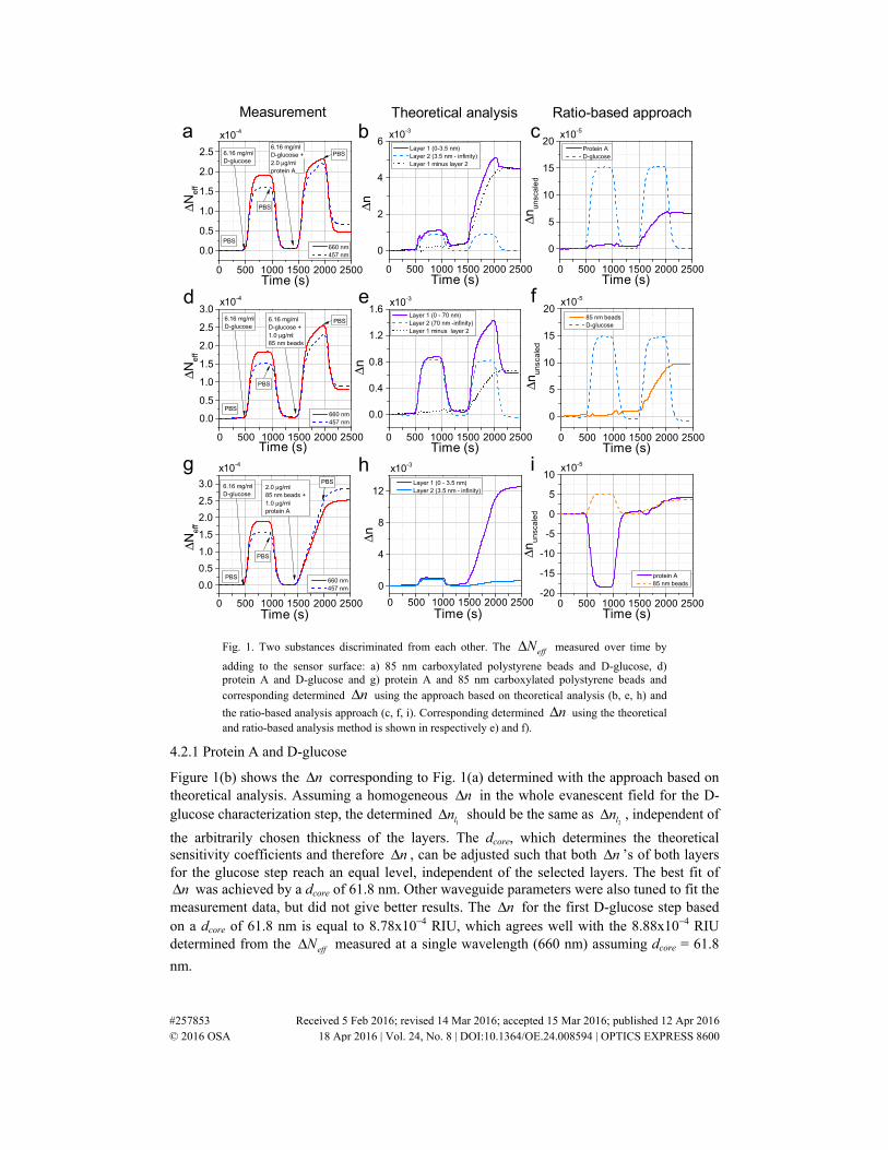
In this section we present measurements where two of the three named different-sized substances (protein A, 85 nm beads and D-glucose which induces a homogeneous nΔ in the whole evanescent field of a few hundreds of nanometres) are discriminated from each other. First, 6.16 mg/ml D-glucose and 2.0 μg/ml protein A were added simultaneously to the sensor (see Fig. 1(a)) and effNΔ is measured at 1λ = 457 nm and 2λ = 660 nm. As a characterization

step 6.16 mg/ml D-glucose only was added to the sensor, which results in an increase of the

effNΔ as D-glucose has a higher n than PBS. As expected, the effNΔ is the highest at 2λ as it

is more sensitive to bulk changes (D-glucose does hardly bind to the surface) compared to 1λ .

After applying a washing step, the effNΔ comes back to zero as the D-glucose bulk solution is

completely replaced by PBS. After simultaneously adding D-glucose and protein A the effNΔ

increases again differently at 1λ compared to 2λ . For both effNΔ ’s the increase consist of a

steep slope due to the bulk effect and a less steep slope due to the binding of the protein A to the surface. After again applying a washing step the signal drops due to the fact that the D-glucose and protein A in the bulk are replaced by PBS. The effNΔ does not go back to zero as

protein A is left at the surface. In this case the effNΔ at 1λ is higher than at 2λ which is

expected since shorter wavelengths are more confined to the core of the waveguide and have a relative larger field near the surface compared to the longer wavelengths. Therefore, the shorter wavelengths are more sensitive to changes close to the surface compared to longer wavelengths. Figure 1(d) shows a similar experiment where after addition of only 6.16 mg/ml D-glucose, 6.16 mg/ml D-glucose was added simultaneously with 1.0 μg/ml 85 nm beads. Figure 1(g) shows a similar measurement where after addition of only 6.16 mg/ml D-glucose,1.0 μg/ml protein A was added simultaneously with 2.0 μg/ml 85 nm beads respectively.


0 500 1000 1500 2000 2500

0.0

0.5

1.0

1.5

2.0

2.5

0 500 1000 1500 2000 2500

0

2

4

6

0 500 1000 1500 2000 2500

0

5

10

15

20

0 500 1000 1500 2000 2500

0.0

0.5

1.0

1.5

2.0

2.5

3.0

0 500 1000 1500 2000 2500

0.0

0.4

0.8

1.2

1.6

0 500 1000 1500 2000 2500

0

5

10

15

20

0 500 1000 1500 2000 2500

0.0

0.5

1.0

1.5

2.0

2.5

3.0

0 500 1000 1500 2000 2500

0

4

8

12

0 500 1000 1500 2000 2500-20

-15

-10

-5

0

5

10

Ratio-based approachTheoretical analysis

i

f

c

e

b

hg

d

ΔNef

f

Time (s)

660 nm 457 nm

x10-4

6.16 mg/mlD-glucose

PBS

PBS

PBS6.16 mg/mlD-glucose + 2.0 μg/ml protein A

Measurement

x10-3

Δn

Time (s)

Layer 1 (0-3.5 nm) Layer 2 (3.5 nm - infinity) Layer 1 minus layer 2

x10-5

Δnun

sca

led

Time (s)

Protein A D-glucose

6.16 mg/mlD-glucose + 1.0 μg/ml 85 nm beads

6.16 mg/mlD-glucose

x10-4

ΔNe

ff

Time (s)

660 nm 457 nm

PBS

PBS

PBS

x10-3

Δn

Time (s)

Layer 1 (0 - 70 nm) Layer 2 (70 nm -infinity) Layer 1 minus layer 2

a

x10-5

Δnu

nsc

ale

d

Time (s)

85 nm beads D-glucose

x10-4

ΔNe

ff

Time (s)

660 nm 457 nm

6.16 mg/mlD-glucose

2.0 μg/ml 85 nm beads + 1.0 μg/ml protein A

PBS

PBS

PBS

x10-3

Δn

Time (s)

Layer 1 (0 - 3.5 nm) Layer 2 (3.5 nm - infinity)

x10-5

Δnu

nsc

ale

d

Time (s)

protein A 85 nm beads

Fig. 1. Two substances discriminated from each other. The effNΔ measured over time by

adding to the sensor surface: a) 85 nm carboxylated polystyrene beads and D-glucose, d) protein A and D-glucose and g) protein A and 85 nm carboxylated polystyrene beads and corresponding determined nΔ using the approach based on theoretical analysis (b, e, h) and

the ratio-based analysis approach (c, f, i). Corresponding determined nΔ using the theoretical and ratio-based analysis method is shown in respectively e) and f).

4.2.1 Protein A and D-glucose

Figure 1(b) shows the nΔ corresponding to Fig. 1(a) determined with the approach based on theoretical analysis. Assuming a homogeneous nΔ in the whole evanescent field for the D-glucose characterization step, the determined

1lnΔ should be the same as

2lnΔ , independent of

the arbitrarily chosen thickness of the layers. The dcore, which determines the theoretical sensitivity coefficients and therefore nΔ , can be adjusted such that both nΔ ’s of both layers for the glucose step reach an equal level, independent of the selected layers. The best fit of

nΔ was achieved by a dcore of 61.8 nm. Other waveguide parameters were also tuned to fit the measurement data, but did not give better results. The nΔ for the first D-glucose step based on a dcore of 61.8 nm is equal to 8.78x10−4 RIU, which agrees well with the 8.88x10−4 RIU determined from the effNΔ measured at a single wavelength (660 nm) assuming dcore = 61.8

nm.


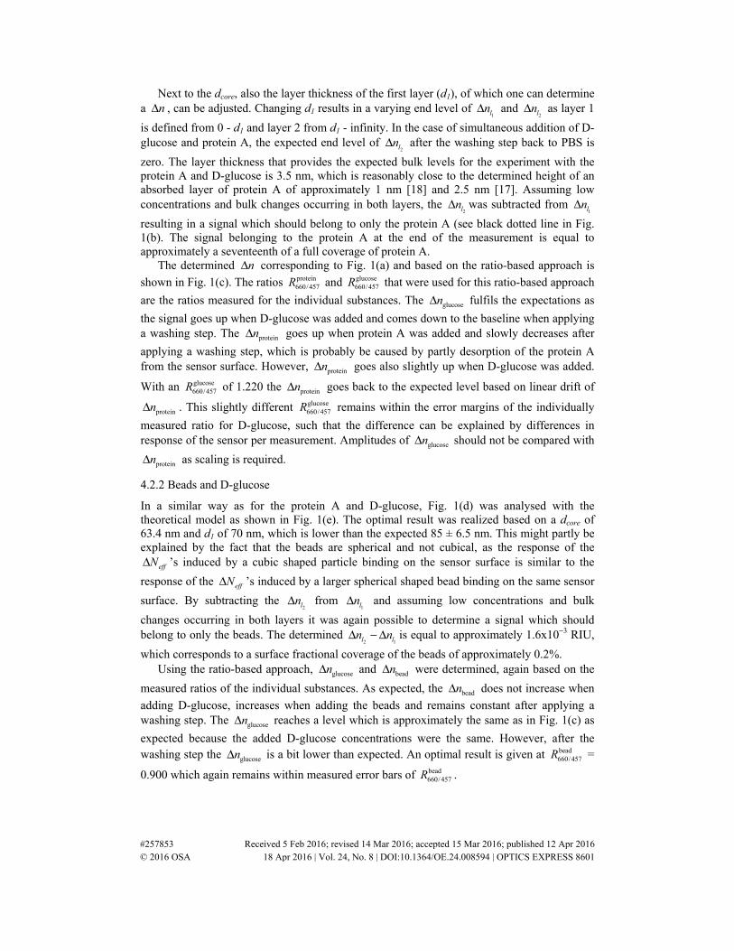
Next to the dcore, also the layer thickness of the first layer (d1), of which one can determine a nΔ , can be adjusted. Changing d1 results in a varying end level of

1lnΔ and

2lnΔ as layer 1

is defined from 0 - d1 and layer 2 from d1 - infinity. In the case of simultaneous addition of D-glucose and protein A, the expected end level of

2lnΔ after the washing step back to PBS is

zero. The layer thickness that provides the expected bulk levels for the experiment with the protein A and D-glucose is 3.5 nm, which is reasonably close to the determined height of an absorbed layer of protein A of approximately 1 nm [18] and 2.5 nm [17]. Assuming low concentrations and bulk changes occurring in both layers, the

2lnΔ was subtracted from

1lnΔ

resulting in a signal which should belong to only the protein A (see black dotted line in Fig. 1(b). The signal belonging to the protein A at the end of the measurement is equal to approximately a seventeenth of a full coverage of protein A.

The determined nΔ corresponding to Fig. 1(a) and based on the ratio-based approach is

shown in Fig. 1(c). The ratios protein660/457R and glucose

660/457R that were used for this ratio-based approach

are the ratios measured for the individual substances. The glucosenΔ fulfils the expectations as

the signal goes up when D-glucose was added and comes down to the baseline when applying a washing step. The proteinnΔ goes up when protein A was added and slowly decreases after

applying a washing step, which is probably be caused by partly desorption of the protein A from the sensor surface. However, proteinnΔ goes also slightly up when D-glucose was added.

With an glucose660/457R of 1.220 the proteinnΔ goes back to the expected level based on linear drift of

proteinnΔ . This slightly different glucose660/457R remains within the error margins of the individually

measured ratio for D-glucose, such that the difference can be explained by differences in response of the sensor per measurement. Amplitudes of glucosenΔ should not be compared with

proteinnΔ as scaling is required.

4.2.2 Beads and D-glucose

In a similar way as for the protein A and D-glucose, Fig. 1(d) was analysed with the theoretical model as shown in Fig. 1(e). The optimal result was realized based on a dcore of 63.4 nm and d1 of 70 nm, which is lower than the expected 85 ± 6.5 nm. This might partly be explained by the fact that the beads are spherical and not cubical, as the response of the

effNΔ ’s induced by a cubic shaped particle binding on the sensor surface is similar to the

response of the effNΔ ’s induced by a larger spherical shaped bead binding on the same sensor

surface. By subtracting the 2l

nΔ from 1l

nΔ and assuming low concentrations and bulk

changes occurring in both layers it was again possible to determine a signal which should belong to only the beads. The determined

2 1l ln nΔ − Δ is equal to approximately 1.6x10−3 RIU,

which corresponds to a surface fractional coverage of the beads of approximately 0.2%. Using the ratio-based approach, glucosenΔ and beadnΔ were determined, again based on the

measured ratios of the individual substances. As expected, the beadnΔ does not increase when

adding D-glucose, increases when adding the beads and remains constant after applying a washing step. The glucosenΔ reaches a level which is approximately the same as in Fig. 1(c) as

expected because the added D-glucose concentrations were the same. However, after the washing step the glucosenΔ is a bit lower than expected. An optimal result is given at bead

660/457R =

0.900 which again remains within measured error bars of bead660/457R .


4.2.3 Protein A and beads

For the measurement of simultaneous addition of beads and protein A the approach based on theoretical analysis is not very suitable, especially because

2lnΔ is far from homogeneous as

the evanescent field penetrates deeper than the thickness of the bead. Moreover, the expected end levels of the protein A and the beads are not known which was known for the bulk effect of the D-glucose. Consequently, the fitting of d1 is not feasible.

Using the ratio-based approach it is possible to discriminate between the protein A and the beads. The result based on ratios of ratios measured for the individual substances is shown in Fig. 1(i). As was mentioned, amplitudes between proteinnΔ and beadnΔ should not be compared

as scaling factors of substances are individual. However, proteinnΔ of Fig. 1(i) can be compared

with proteinnΔ of Fig. 1(c). In Fig. 1(i) half of protein A was added to the sensor, but the

measured proteinnΔ is only 1.6 times lower. An even lower signal of proteinnΔ is expected as

now also beads can cover part of the surface where beads can bind. Furthermore, the beadnΔ of

Fig. 1(f) is approximately 2.6 times higher compared to beadnΔ of Fig. 1(i), where the added

beads concentration was two times lower. The differences might be explained that different chips and different stock solutions were used for the different measurements. Furthermore, all the measurements are based on the non-specific adhesion of the protein A and the beads to the sensor surface. Therefore, small differences between sensor surfaces can make a large difference. The result from D-glucose in which no binding is involved, the signals were in nice agreement with each other. Determined RI changes due to non-specific binding of particles and between different measurements should not be compared if not all the conditions (chip, stock solution, analysis parameters) of the measurements are the same.

Besides, Fig. 1(i) shows that using two ratios, excluding glucose660/457R , it is not possible to

suppress the first D-glucose step from the protein and beads signal. Three wavelengths are required to discriminate between protein A, 85 nm beads and D-glucose in a single measurement, as presented in the Appendix C.

4.3 Blind experiment

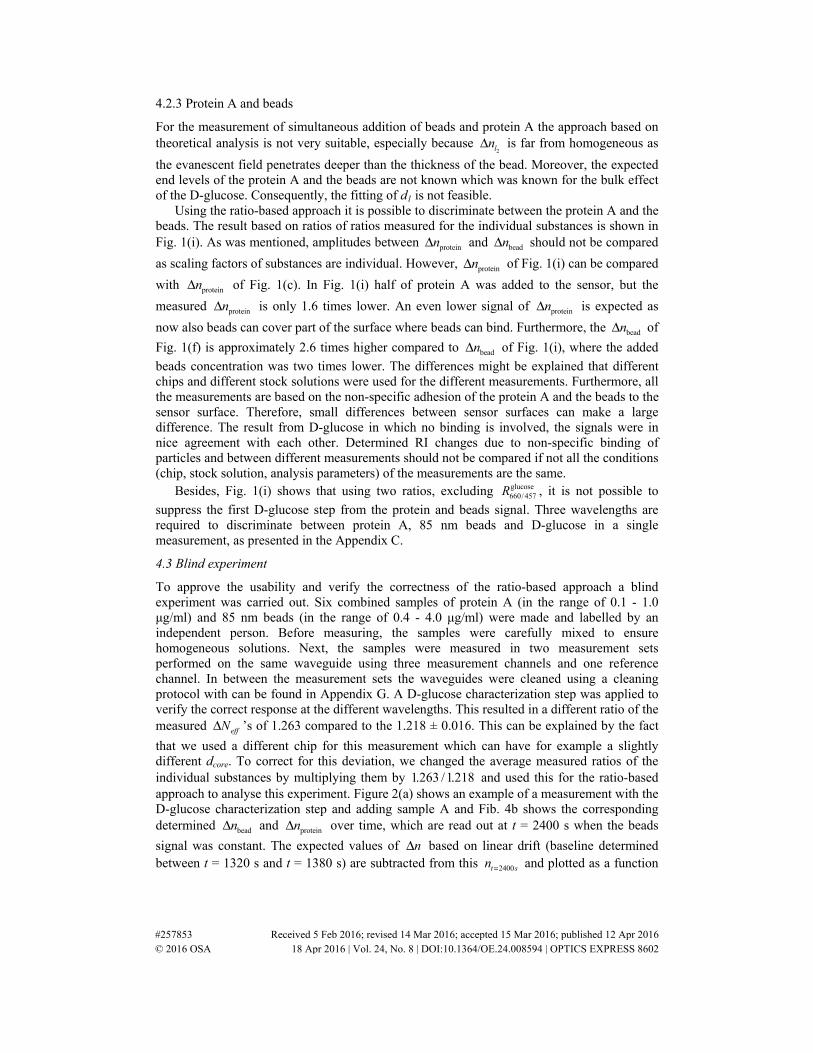
To approve the usability and verify the correctness of the ratio-based approach a blind experiment was carried out. Six combined samples of protein A (in the range of 0.1 - 1.0 μg/ml) and 85 nm beads (in the range of 0.4 - 4.0 μg/ml) were made and labelled by an independent person. Before measuring, the samples were carefully mixed to ensure homogeneous solutions. Next, the samples were measured in two measurement sets performed on the same waveguide using three measurement channels and one reference channel. In between the measurement sets the waveguides were cleaned using a cleaning protocol with can be found in Appendix G. A D-glucose characterization step was applied to verify the correct response at the different wavelengths. This resulted in a different ratio of the measured effNΔ ’s of 1.263 compared to the 1.218 ± 0.016. This can be explained by the fact

that we used a different chip for this measurement which can have for example a slightly different dcore. To correct for this deviation, we changed the average measured ratios of the individual substances by multiplying them by 1.263 /1.218 and used this for the ratio-based approach to analyse this experiment. Figure 2(a) shows an example of a measurement with the D-glucose characterization step and adding sample A and Fib. 4b shows the corresponding determined beadnΔ and proteinnΔ over time, which are read out at t = 2400 s when the beads

signal was constant. The expected values of nΔ based on linear drift (baseline determined between t = 1320 s and t = 1380 s) are subtracted from this 2400t sn = and plotted as a function


of the applied concentration in Fig. 2(c) and Fig. 2(d) for the 85 nm beads and the protein A respectively.

0 1000 2000

0

2

4

6

8

10

0 1000 2000-2

0

2

4

6

0.0 0.2 0.4 0.6 0.8 1.00.0

0.5

1.0

1.5

2.0

2.5

0 1 2 3 40

4

8

12

x10-4

ΔNe

ff

Time (s)

660 nm 457 nm

PBS

6.16 mg/mlD-glucose sample A

PBS

PBS

x10-4

Δnun

sca

led (

a.u.

)

Time (s)

protein A 85 nm beads

c d x10-4

A

FD

B

E

C

Mea

sure

d Δn

(a.

u.)

Applied concentration (μg/ml)

Protein Ax10-4

b

85 nm beads

B

E

D

F

C

Mea

sure

d Δn

(a.

u.)

Applied concentration (μg/ml)

A

a

Fig. 2. Blind experiment with six samples (A-F) containing 85 nm beads and protein A. a) The

measured effNΔ over time of one measurement of the set of blind experiments b) the

corresponding determined beadsnΔ and proteinnΔ using the ratio-based approach and c) the

determined nΔ as a function of the by forehand unknown applied concentrations of the 85 nm

beads and d) the determined nΔ as a function of the by forehand unknown applied concentrations of the protein A. For visibility reasons, the data points A and F of the applied protein concentration are slightly offset but they both correspond to 0.9 μg/ml.

The applied bead concentration and the determined beadnΔ show a linear trend which

means the beadnΔ was determined correctly using the ratio-based approach, assuming a linear

relation between the number of beads in the sample and response of the sensor. Moreover, it shows that it is possible to do a calibration experiment to find the relations between the beads concentration and the response of the sensor. Furthermore, also a linear trend is seen between the measured proteinnΔ and the applied protein concentration. Only at higher applied protein A

concentrations, the determined proteinnΔ flattens off, which can be explained by the fact that

for these measurements the surface was saturated with protein A which can be seen in Fig. 2(b). That the signal of beadnΔ still increases might be explained by the beads replacing the

protein A of the surface. The be able to compare beadnΔ and proteinnΔ , the signals were both

read out at the same time point. The blind experiment illustrates that the determined substancenΔ


can be compared with the substancenΔ of a different experiment, when using the same

measurement conditions (chip, stock solution, analysis parameters).

4.4 Noise, drift and artefacts in measurements

Here, we shortly discuss the influence noise, drift and artefacts in effNΔ on nΔ . All noise

sources in the signal of effNΔ are enhanced using the above named approaches, which means

that they are stronger visible in nΔ . This can be explained by the matrix becoming more singular, resulting in enhancement of all kind of noise sources. Linear drift measured in

effNΔ ’s (e.g. due to temperature changes causing relative movement between chip and CCD

camera or causing directly a nΔ at the sensing windows) results in linear drift in nΔ of both layers (see Appendix E). For the measurements we assume linear drift and take this into

account when fitting /m

k l

sRλ λ or waveguide parameters. Moreover, artefacts (fluctuations e.g.

seen in Fig. 1(f) at t ≈500 s and 1000 s in proteinnΔ , but better visible at discrimination between

three substances using three wavelengths, see Appendix C) show up in nΔ . These artefacts are present in the signal of the effNΔ ’s, but are not visible because of the relatively higher

slopes of effNΔ due to the fast addition of the sample. The artefacts are caused by boundary

effects of the shifting interference pattern (see Appendix D). When inducing a linear ϕΔ in

the interference pattern this results in a oscillation in the amplitude of the spatial frequency as it is not constant when the fringes move. It also results in a oscillation in ϕΔ which is

directly related to effNΔ . Using a proper windowing function (e.g. Blackman-Nuttall) we

were able to remove the oscillations from simulated shifting interference patterns. However, this was not sufficient for the measured data, possibly because of non-ideal properties of the

lenses, the grating and beam shape (see Appendix D). Therefore, the artefacts in effNΔ can

result in misfits of the fitted /m

k l

sRλ λ or waveguide parameters. The spread in the determined

dcore, dlayer and /m

k l

sRλ λ can be caused by especially the artefacts, resulting in a wrongly

determined nΔ . The signal of nΔ becomes especially very noisy in the case when discriminating between three nΔ ‘s based on three effNΔ ‘s (see Appendix C). To be able to

use this method for three wavelengths to solve three independent nΔ ’s, the artefacts in the measurement should be reduced by for example testing if larger optical components reduce the artefacts.

5. Summary and conclusions

By measuring the effNΔ at two different wavelengths it was possible to discriminate between

two different substances inducing a nΔ in the evanescent field of the sensor. The binding of 85 nm beads or protein A was discriminated from D-glucose and the binding of 85 nm beads was discriminated from the binding of protein A. Using three effNΔ ’s to discriminate between

three different substances inducing a nΔ , the result became more noisy. For a successful application of these analysis approaches used to determine three independent nΔ ’s, the artefacts (due to boundary effects of the shifting interference pattern, see Appendix D) in

effNΔ should be reduced significantly. Alternatively, other techniques to improve specificity

can be used next to size-selective detection. For example, to discriminate the binding of beads from binding of protein A and bulk changes due to D-glucose, D-glucose can also be added to


the reference channel to cancel out the contribution due to D-glucose. In that case only two wavelengths are required to discriminate between binding of beads and proteins, resulting in less enhancement of noise.

Application of a approach based on theoretical analysis made it possible to discriminate between nΔ ’s occurring in different layers in the evanescent field, assuming a homogeneous

nΔ in each layer. However, to determine the correct value for nΔ , this method requires multiple parameters (e.g. the waveguide core thickness, waveguide RIs, layer thicknesses, wavelengths) to be tuned that is difficult and labour-intensive. Therefore, also a much more pragmatic ratio-based analysis approach is presented to discriminate between nΔ ’s induced by different substances. Moreover, this approach can be used for different substances inducing a nΔ in overlapping layers, which is not always possible with the approach based on theoretical analysis. Information on the absolute amplitude of snΔ is lost using the ratio-based

approach, however for determining an analyte concentration calibration measurements can be performed which are usually also required using an YI with a single wavelength. 85 nm beads, D-glucose and protein A were discriminated from each other using this ratio-based approach. The working of the ratio-based approach was verified by a blind experiment with different samples containing different concentrations of protein A and beads. We could discriminated beadnΔ from proteinnΔ , resulting in an expected linear trend of the beadnΔ with the

applied concentration. So here we discriminate between protein A (≈2 nm large) and 85 nm beads, but this can raise the question what would be the minimal size difference of discriminable substances. It is very difficult to say something general about this as the minimal discriminable size difference depends on a number of parameters such as the amplitude of the signals of the substances and the amplitude of the noise, artefacts and drift of the phase signal. When a certain application is identified, then the sensor should be optimized to determine the limits of the device for the specific application in mind. Size-selective analyte detection can for example be used to discriminate specific analyte binding of larger particles from non-specific binding of smaller particles. Therefore, we believe that with measuring size-selectivity we can strongly improve the performance of our YI sensor and IO interferometric sensors in general. Especially the ratio-based approach is an easy approach to discriminate between different substances causing a nΔ .

Appendix A: Experimental details

In this section we describe the experimental details of the setup which was used for the measurements presented in the main text and in the rest of the appendices.

A.1 Sample transportation

Samples are degassed by a 4-channel Degassi Classic degasser and transported to the sensor surface by a 4-channel Ismatec® Reglo Digital Peristaltic Pump with a flow rate of 100 μl/min towards the sensing windows of the waveguide structure. On top of these sensing windows a 100 μm high fluid cuvette is placed to transport the sample to the sensor with a laminar flow, which means that in the evanescent field that is used for detection the velocity is nearly zero and transport of the different substances is determined by diffusion.

A.2 Hardware

Measurements are performed in a 4-channel single-mode ridge waveguide YI sensor. The waveguide consists three layers: a PECVD SiO2 layer covering a LPCVD Si3N4 70 nm thick core on top of a thermal SiO2 substrate. A sensing window with a length l of 4 mm is created by etching away the PECVD SiO2 cover. Measurements are done with one single waveguide structure (chip) which is cleaned after each measurement (see Appendix G). The wavelengths 457, 561 (only used when discriminating between three substances) and 660 nm are chosen such that only zero order TE modes (in height) fit into the waveguide and such that


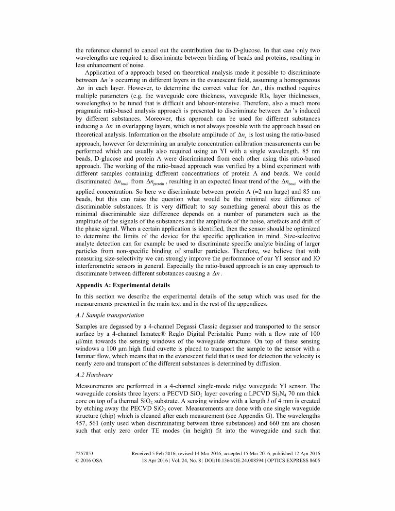
wavelengths are well spread, which is required to achieve a good precision [15]. The different light sources are coupled into a single mode polarization maintaining (SMPM) fiber which can be positioned with respect to the waveguide using an xyz-stage to be able to quickly and sufficiently couple all wavelengths into the waveguide. The fiber tip is strengthened with a glass ferule which is positioned against the waveguide with a matching index gel in between them to prevent reflections at the interfaces which resulted in a oscillations of the phase signal. Figure 3 shows a schematic overview of the hardware of the setup.

Fig. 3. Setup. Schematic overview of the setup where L1-L3 are a 50 mW Cobolt Twist 457 nm Single Longitudinal Mode (SLM) Diode-Pumped Solid State (DPSS) laser, a 50 mW Cobolt Jive 561 nm SLM DPSS laser and a 50 mW Cobolt Flamenco 660 nm SLM DPPS laser respectively of which the power is regulated using Thorlabs NDC-100C-4M mounted variable ND filters (N1-N3) of which the reflected light is directed to Thorlabs BT500 beam dumps. Next, Thorlabs, BB1-E02 visible broadband dielectric mirrors (M1-M4) and a Semrock Di01-R561-25x36 dichroic mirror (D1) and a Semrock Di01-R442-25x36 dichroic mirror (D2) are used to overlap the three lasers which are subsequently coupled into a Thorlabs PM460-HP single mode polarization maintaining (SMPM) fiber using a Schäfter + Kirchhoff GmbH 60FC-4-RGBV11-47 apochromatic fiber collimator (F). This fiber is positioned on a ULTRAlign Precision XYZ Positioning Stage (XYZ) with DS-4F High Precision Adjusters to position the fiber with respect to the YI waveguide (W) in order to efficiently couple the light via butt-end coupling into this 4-channel single-mode ridge waveguide. After the light is coupled out of the waveguide it will form an interference pattern which is collimated in the horizontal plane using a Thorlabs, ACY254-075-A cylindrical achromatic lens (C1). Subsequently, the interference pattern passes a Thorlabs LPVISE100-A linear polarizer with 400-700 nm N-BK7 protective windows (P) to filter out possible converted TM polarized light. Next, the light is directed to a Thorlabs, GT-25-03 25mm x 25mm 300 lines/mm visible transmission grating (G) to separate the different wavelengths after which it passes a Thorlabs ACY254-050-A cylindrical achromatic lens (C2) which images the interference patterns on a Alta U30-OE CCD camera (CCD).

A.3 Analysis

A Fast Fourier Transform (FFT) is applied to the interference patterns detected with the CCD camera. Different windows were applied to the interference patterns to prevent boundary effects (see Appendix D). Subsequently, spatial frequency peaks of the interference pattern are determined such that the phase change ϕΔ ( effN∝ Δ ) of each channels pair can be read

out. For the measurements we only use one channel pair combination (one measurement channel and one reference channel) and the rest is neglected, expect for the blind experiment for which we use all channels.


Appendix B. Ratio-based analysis approach

B.1 Effective refractive index ratios at various wavelengths

The ratios /m

n m

sRλ λ are experimentally determined for three different wavelengths ( 1λ =457 nm,

2λ =561 nm and 3λ =660 nm), and for three different substances: 85 nm carboxylated

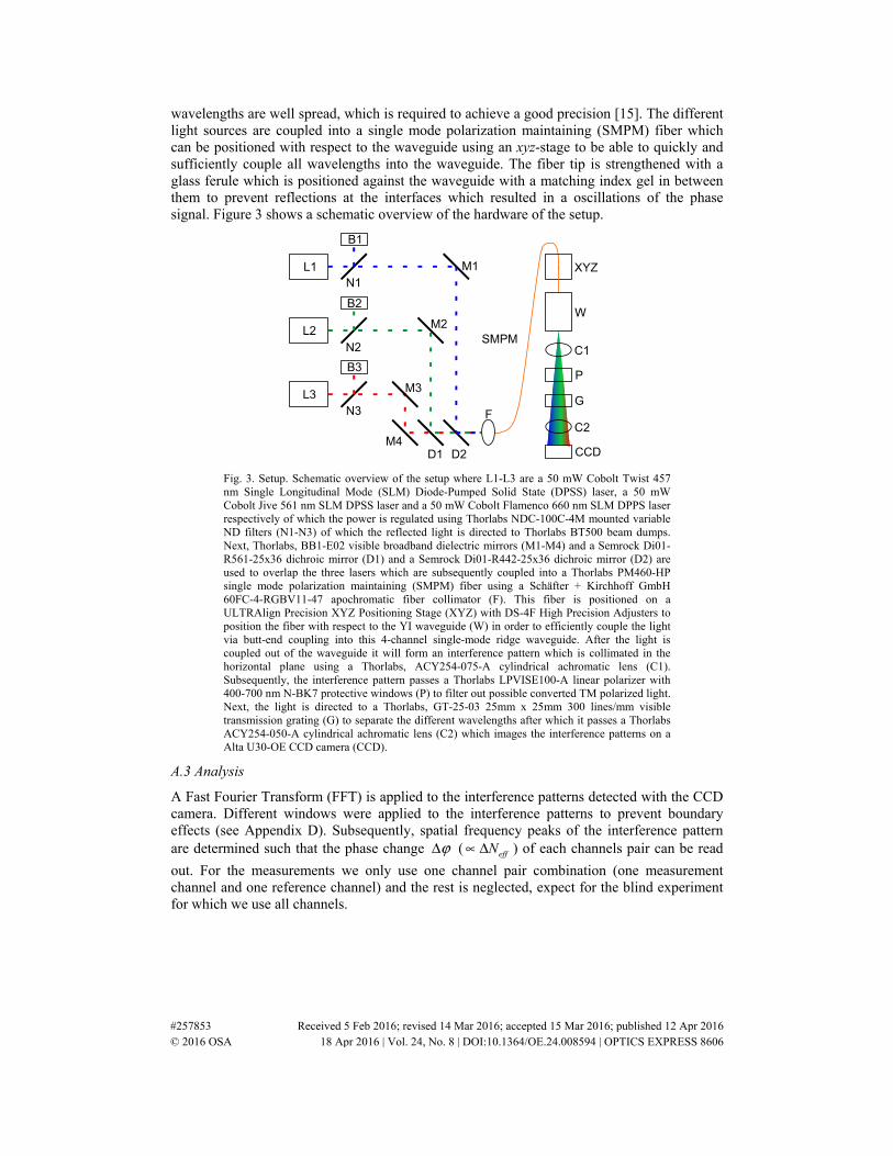
polystyrene beads, protein A and D-glucose (see Table 1), representing specific binding, non-specific binding and bulk changes respectively. Figure 4 shows an example of a measurement with D-glucose and 85 nm beads measured at 1λ =457 nm and 3λ =660 nm, illustrating the

difference in 660/457R for both substances. A single value for the ratio for a given substance is

determined by calculating the mean value of the ratios over the time interval in which the ratios have a relatively stable value for that substance. In practice it was found that the time intervals that show a stable ratio correspond to intervals in which

1,effN λ was between 80 -

100% of its maximum value for D-glucose, 20 - 100% for 85 nm beads and 10 - 100% for protein A. Therefore these intervals were applied for determination of all ratios.

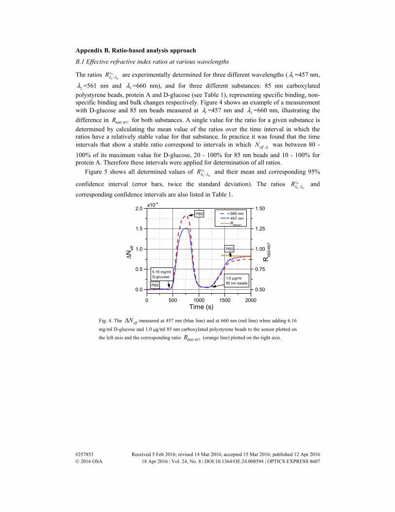
Figure 5 shows all determined values of /m

n m

sRλ λ and their mean and corresponding 95%

confidence interval (error bars, twice the standard deviation). The ratios /m

n m

sRλ λ and

corresponding confidence intervals are also listed in Table 1.

0 500 1000 1500 2000

0.0

0.5

1.0

1.5

2.0

1.0 μg/ml 85 nm beads

PBS

PBS

PBS

ΔNe

ff

Time (s)

660 nm 457 nm

R660/457

6.16 mg/ml D-glucose

0.50

0.75

1.00

1.25

1.50

R6

60

/45

7

x10-4

Fig. 4. The effNΔ measured at 457 nm (blue line) and at 660 nm (red line) when adding 6.16

mg/ml D-glucose and 1.0 μg/ml 85 nm carboxylated polystyrene beads to the sensor plotted on

the left axis and the corresponding ratio 660/457R (orange line) plotted on the right axis.


0.6

0.8

1.0

1.2

1.4

R85 nm beadsProtein A D-Glucose

660/457 561/457 660/561

Fig. 5. Measured ratios /n m

sRλ λ (dots, diamonds and triangles) for protein A, 85 nm

carboxylated polystyrene beads and D-glucose for all combinations of the wavelengths 457 nm, 561 nm and 660 nm. Also indicated is the average of the measured ratios and the corresponding error bars representing the 95% confidence interval.

Table 1. Measured effective refractive index ratios. Experimentally determined effNΔ

ratios at 1λ = 457 nm, 2λ = 561 nm and 3λ = 660 nm determined for D-glucose, 85 nm

carboxylated polystyrene beads and protein A.

660/457R 561/457R 660/561R

D-glucose 1.218 ± 0.016 1.160 ± 0.012 1.050 ± 0.008 85 nm beads 0.918 ± 0.045 0.998 ± 0.037 0.920 ± 0.040 Protein A 0.680 ± 0.022 0.830 ± 0.022 0.820 ± 0.023

B.2 Theory of ratio-based analysis method

Here, we derive Eq. (3) of the manuscript. When a substance sm is added to the sensor it induces a sm

nΔ , this results in an effective refractive index change , keffN λΔ at kλ . Assuming

that the response of the sensor has a linear relationship with the amount of sm that is added to the sensor, this can be written as:

,

, ss

,k

k m

m

eff

eff

NN n

nλ

λ

∂Δ = Δ

∂ (4)

where , sk meffN nλ∂ ∂ is the sensitivity coefficient of the sensor for a RI change induced by sm.

Assuming that substances do not influence each other’s response of the sensor, multiple substances inducing different ratios can be discriminated from each other using:

s ,eff subN S nΔ = ⋅ Δ (5)

where the vector effNΔ is composed of the elements keff,N λΔ , the vector snΔ is composed of

the elements msnΔ , and the coefficients of matrix subS are given by , , sk mk m effs N nλ= ∂ ∂ .

Next, we define the ratio of two effNΔ ’s measured at two wavelengths kλ and lλ , induced

by a substance sm as:


, ,

, ,

,/

,

.m m

eff eff m mk km

k l m m

eff eff m ml l

s ss s k ms

s sl ms s

N N n n sR

sN N n nλ λ

λ λ

λ λ

Δ ∂ ∂ ⋅ Δ= = =

Δ ∂ ∂ ⋅ Δ (6)

where we neglect the dispersion in msnΔ . We can express the elements of matrix subS in

terms of the ratios /m

k l

sRλ λ . Due to the fact that / /1m m

k l l k

s sR Rλ λ λ λ= and / / /m m m

k l k j l j

s s sR R Rλ λ λ λ λ λ= we

can rewrite Eq. (5) as:

s ,effN R nΔ = ⋅Θ⋅ Δ (7)

where Θ is a matrix with theoretical sensitivity coefficients of which the elements are given

by , ,k mk m s k mSλθ ∀= = and , 0k m k mθ = ∀ ≠ , and the coefficients of matrix R are given by

, /m

k m

sk mr Rλ λ= . To determine snΔ Eq. (7) can be rewritten as:

1 1

s .effn R N− −

Δ = Θ ⋅ ⋅ Δ (8)

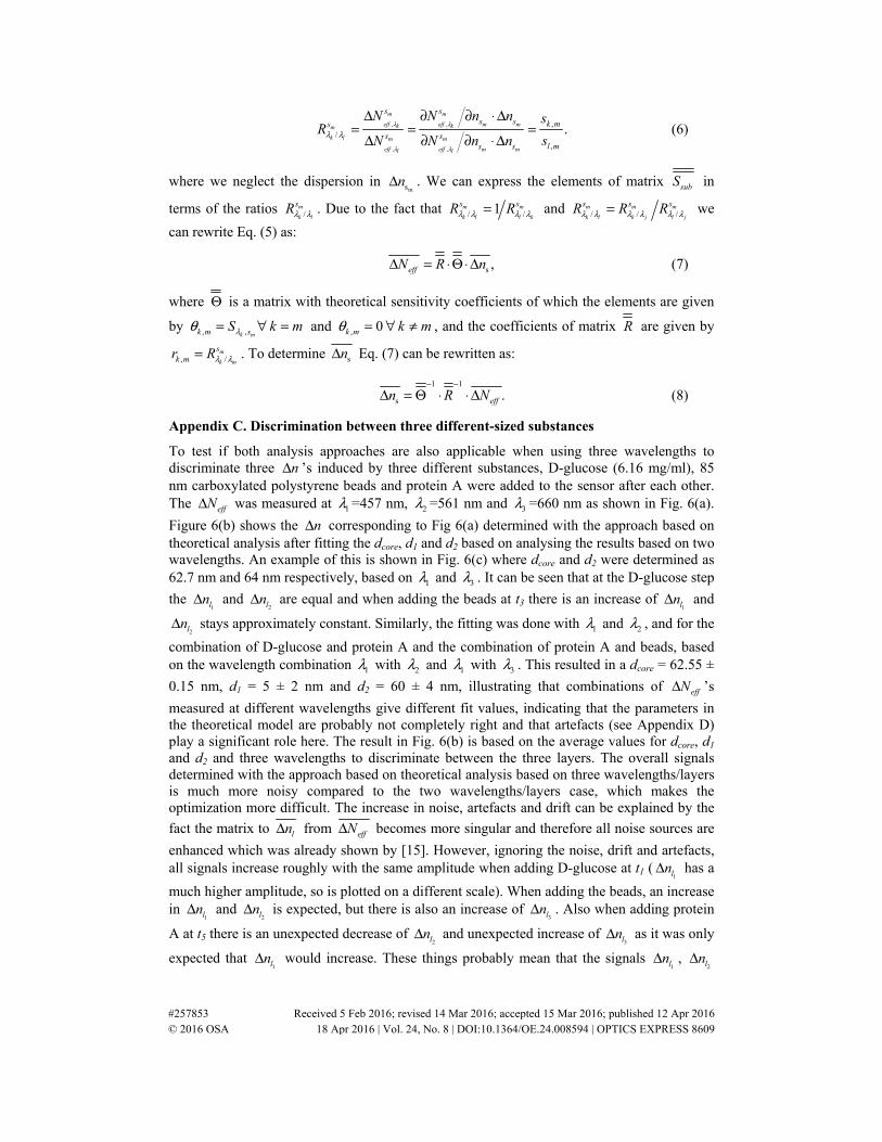
Appendix C. Discrimination between three different-sized substances

To test if both analysis approaches are also applicable when using three wavelengths to discriminate three nΔ ’s induced by three different substances, D-glucose (6.16 mg/ml), 85 nm carboxylated polystyrene beads and protein A were added to the sensor after each other. The effNΔ was measured at 1λ =457 nm, 2λ =561 nm and 3λ =660 nm as shown in Fig. 6(a).

Figure 6(b) shows the nΔ corresponding to Fig 6(a) determined with the approach based on theoretical analysis after fitting the dcore, d1 and d2 based on analysing the results based on two wavelengths. An example of this is shown in Fig. 6(c) where dcore and d2 were determined as 62.7 nm and 64 nm respectively, based on 1λ and 3λ . It can be seen that at the D-glucose step

the 1l

nΔ and 2l

nΔ are equal and when adding the beads at t3 there is an increase of 1l

nΔ and

2lnΔ stays approximately constant. Similarly, the fitting was done with 1λ and 2λ , and for the

combination of D-glucose and protein A and the combination of protein A and beads, based on the wavelength combination 1λ with 2λ and 1λ with 3λ . This resulted in a dcore = 62.55 ±

0.15 nm, d1 = 5 ± 2 nm and d2 = 60 ± 4 nm, illustrating that combinations of effNΔ ’s

measured at different wavelengths give different fit values, indicating that the parameters in the theoretical model are probably not completely right and that artefacts (see Appendix D) play a significant role here. The result in Fig. 6(b) is based on the average values for dcore, d1 and d2 and three wavelengths to discriminate between the three layers. The overall signals determined with the approach based on theoretical analysis based on three wavelengths/layers is much more noisy compared to the two wavelengths/layers case, which makes the optimization more difficult. The increase in noise, artefacts and drift can be explained by the

fact the matrix to lnΔ from effNΔ becomes more singular and therefore all noise sources are

enhanced which was already shown by [15]. However, ignoring the noise, drift and artefacts, all signals increase roughly with the same amplitude when adding D-glucose at t1 (

1lnΔ has a

much higher amplitude, so is plotted on a different scale). When adding the beads, an increase in

1lnΔ and

2lnΔ is expected, but there is also an increase of

3lnΔ . Also when adding protein

A at t5 there is an unexpected decrease of 2l

nΔ and unexpected increase of 3l

nΔ as it was only

expected that 1l

nΔ would increase. These things probably mean that the signals 1l

nΔ , 2l

nΔ


and 3l

nΔ are not sufficiently decoupled. Optimizing the theoretical matrix further is more

complex compared to the two wavelengths/layers situation, because changing one parameter will result in change of all the signals

1lnΔ ,

2lnΔ and

3lnΔ , illustrating the complexity and

limits of the approach based on theoretical analysis. Therefore, we ratio-based approach is better used for this analysis.

0 1000 2000 3000

0

1

2

3

4

5

0 1000 2000 3000

0

1

2

3

0 1000 2000 3000-2

0

2

0 1000 2000 3000-1

0

1

2

3

4

0 1000 2000 3000-1

0

1

2

3

0 1000 2000 3000

0

4

8

12

16

20

t3

t2

t1

ΔNef

f

Time (s)

660 nm 561 nm 457 nm

x10-4

t4t5

t6

x10-4x10-2 cb

Δnla

yer

1

Time (s)

Layer 1 (0 - 3 nm)

t4

t1t3

t2t6

t5

a

d e f

0

2

4

6

8

10

L2 (5 - 60 nm) L3 (60 nm - inf)

Δnla

yer

2, 3

Δn

Time (s)

Layer 1 (0 - 64 nm) Layer 2 (64 nm -inf)

t2t1

t3

t4t6

t5

x10-3

x10-5

Δnu

nsca

led

Time (s)

Protein A 85 nm beads D-glucose

t2

t1

t3

t4

t6

t5

x10-5

Δnu

nsca

led

Time (s)

Protein A 85 nm beads D-glucose

t2

t1 t3t4

t6

t5

x10-5

Δnu

nsca

led

Time (s)

Protein A D-glucose

t2

t1t3

t4

t6

t5

Fig. 6. Three substances discriminated from each other. a) The effNΔ measured over time

starting with a PBS buffer, adding 6.16 mg/ml D-glucose at t1 resulting in higher effNΔ for

the longer wavelengths as expected. After applying a washing step at t2,1.0 μg/ml 85 nm beads was added at t3. The response of the shorter wavelengths is now larger. After washing again with PBS at t4, 2.0 μg/ml protein A was added at t5 resulting in a relatively stronger response of the shorter wavelengths. After applying a washing step at t6 the signal decreases due to

desorption of the protein A, b) the corresponding layernΔ determined with the approach based

on theoretical analysis fitting dcore, d1 and d2 based on analysing the measurement with two

wavelengths (see example shown in c)), the substancenΔ determined with ratio-based approach

based on d) the ratios measured with the individual substances and e) after tuning the ratios based on analysing the measurement with two wavelengths and two substances of which an example is given in f).

Figure 6(d) shows the determined snΔ with the ratio-based approach. The ratios used for

the analysis are again based on the determined ratios of effNΔ at the different wavelengths for

the individual substances. Between t1 and t2 only glucosenΔ changes apart from some

fluctuations seen for beadnΔ and proteinnΔ , which can be explained by boundary effects of the

shifting interference pattern (see section 4.4 Noise, drift and artefacts in measurements in main text). At t3 the beads where added, but besides the increase of beadnΔ there is also an

increase of proteinnΔ and glucosenΔ which means that the signals of snΔ are not perfectly

decoupled. This is also the case at t5 when protein A is added to the sensor which mainly


result in an increase of proteinnΔ , but also in a small increase of glucosenΔ . Therefore, the ratios

were also optimized by analysing the measurement based on two wavelengths/substances. An example is shown in Fig. 6(f), which shows that proteinnΔ was sufficiently decoupled from

glucosenΔ based on 1λ and 3λ . Because only two wavelengths were used to discriminate

between proteinnΔ and glucosenΔ it was not possible to discriminate them from beadnΔ which is

shown between t3 and t4 where both proteinnΔ and glucosenΔ increase. Figure 6(e) shows the

result of snΔ after optimization of the ratios which led to protein561/ 457R =0.837, protein

660/457R =0.698, bead561/ 457R =0.967, bead

660/457R =0.885, glucose561/ 457R =1.158 and glucose

660/457R =1.215 from which s660/561

mR can be

calculated by dividing s660/457

mR by s561/ 457

mR . All these values fall within the error margins of the

experimentally determined ratios of the individual substances presented in Table 1. Using the slightly changed ratios, the three substances are nicely decoupled, illustrating that it is possible to discriminate between three different substances. However, the enhanced drift and

artefacts in snΔ makes it difficult to analyse these results. Moreover, when substances were

added simultaneously (data not shown here) fitting based on two substances/two wavelengths is not possible. Therefore, the ratios used for the analysis should be measurable from measurements with the single substances and not be tuned afterwards. To realise this the spread in ratios should be reduced. More research is required to determine what the origin of the spread of the ratios is. In order to do this, it should be investigated if the spread can be explained by the artefacts or other noise sources of the measurements, the cleaning of the surfaces of the chip (larger spread is seen in binding of substances compared to bulk changes due to D-glucose) or the substances self (spread in protein A is smaller compared to beads). At least it is required to reduce the aforementioned artefacts which are enhanced too much when using three wavelengths to discriminate between three substances.

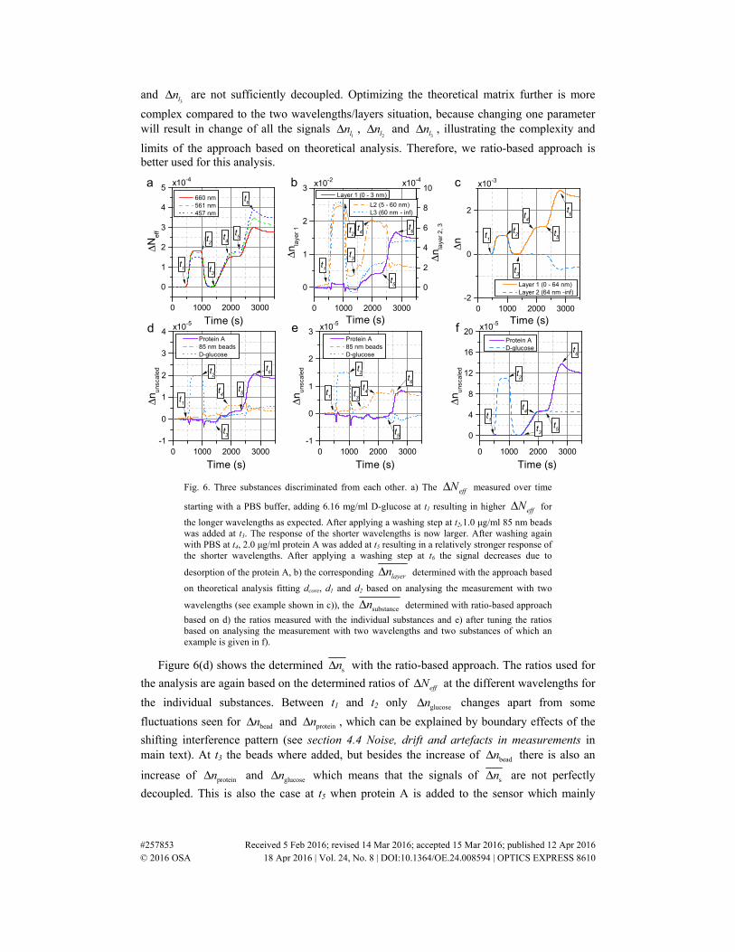
Appendix D. Artefacts in signal due to boundary effects of shifting interference pattern

Computer generated images of interference patterns (based on our four channel Young interferometer) were used to verify the correct working of the Labview program which is used to collect interference patterns and determine the corresponding phase changes during an experiment, to investigate artefacts when determining a phase change from a finite interference pattern and to test windowing functions to reduce artefacts. Calculations of the generated interference patterns are based on four point sources distanced at 60 μm, 80 μm and 100 μm, an imaged distance of 17.5 cm, and wavelengths of 457 nm and 660 nm. The generated images have a width of 1024 pixels, a height of 100 pixels and a dynamic range of 60000 counts and include shot noise (Poisson noise). To simulate a real experiment, a time varying effNΔ (~ ϕΔ ) is introduced (see Fig. 7(a)). For each corresponding time point an

image is calculated and stored for later analysis. Next, the Labview program loads the images, adds up the selected number of rows on which the interference patterns are imaged and subsequently adds 1024 zeros to increase spatial frequency resolution to improve phase readout. Optionally, a windowing function is applied before a Fast Fourier Transform (FFT) is executed. From the resulting spectrum, the phase and amplitude of the six different spatial frequencies are determined of which we now analyse one peak belonging to one channel pair. Figure 7(a) shows an example of the induced and calculated effNΔ for the two wavelengths.

The same figure also shows the difference in effNΔ between the induced and determined

values. Figure 7(b) shows the determined amplitude and Fig. 7(c) shows the substancenΔ

determined with the ratio-based approach based on the induced (ind) and determined (det)

effNΔ . Figure 7(d), 7( e) and 7(f) show the effNΔ , the amplitude and the determined


substancenΔ of a real measurement. Similar fluctuations (which we call artefacts) are seen in in

the amplitude and substancenΔ when no windowing is applied on the simulated interference

patterns. These artefacts are most prominent during (fast) changes in the induced effNΔ .

0 400 800

-2

0

2

4

0 400 80018.0

18.5

19.0

19.5

20.0

0 400 800

0

2

4

6

8

0 1000 2000

0

1

2

3

4

0 1000 20007.6

7.8

8.0

8.2

0 1000 2000

0

2

4

6

8

ΔNe

ff

Time (s)

660, ind 457, ind 660, det 457, det

-1

0

1

2

3

4x10-6

660, det-ind 457, det-ind

x10-4

Δ�ΔN

eff�

Am

plitu

de (

coun

ts)

Time (s)

457 nm 660 nm

Δnun

sca

led

Time (s)

Binding, ind Bulk, ind Binding, det Bulk, det

x10-5

ed f

cb

x10-4

ΔNe

ff

Time (s)

660 nm 457 nm

a

Am

p 66

0 n

m (

coun

ts)

Time (s)

660 nm 1.6

1.8

2.0

2.2

x107

x107x107

457 nm Am

p 457

nm (

coun

ts) x10-5

Δnu

nsc

ale

d

Time (s)

85 nm beads D-glucose

Fig. 7. Comparison of fluctuations in the effNΔ as determined by using simulated data (a,b,c)

and measured data (d,e,f) in a typical measurement composed of a bulk signal followed by a

combination of a bulk signal and a signal arising from surface binding. a) effNΔ induced (ind)

and determined by analysing simulated data without applying a window (det) and the

difference between detected and induced effNΔ , b) the amplitude determined by the FFT

corresponding to the ϕΔ from which effNΔ is determined, c) nΔ as induced and as

determined using the ratio-based approach, d) the effNΔ of a measurement where first D-

glucose was added, followed by adding simultaneously D-glucose and 85 nm beads to the sensor surface, e) the corresponding amplitude of the FFT-spectrum at the measured spatial frequency and f) the determined nΔ due to binding of the beads and bulk changes due to the D-glucose.

To investigate this further, a linear ϕΔ (~ effNΔ ) was induced and the peak-to-peak (pk-

pk) values of the artefacts in effNΔ were determined to test the influence of the applied

window on the size of the artefacts (both in amplitude and ϕΔ (~ effNΔ )). Figure 8(a) shows

the linear effNΔ determined from the linear ϕΔ , and the difference between the determined

and induced effNΔ (= effNΔ error, abbreviated as NE in the remainder of the text) for the case

in which no window is applied and the case in which a in Labview build-in Blackman-Nuttall window is applied. Figure 8(b) shows the mean pk-pk values of the NE of different channel combinations, determined from ϕΔ measured at the spatial frequencies (sf) belonging to the

channel combination in which a nΔ was generated in one of the channels as well as from the channel combinations in which no nΔ occurred (cross-talk, CT). To demonstrate the effect of windowing, results are plotted for different type of windows. For example, applying a Blackman-Nuttall or a Dolph-Chebyshev window, both CT and NE can be completely


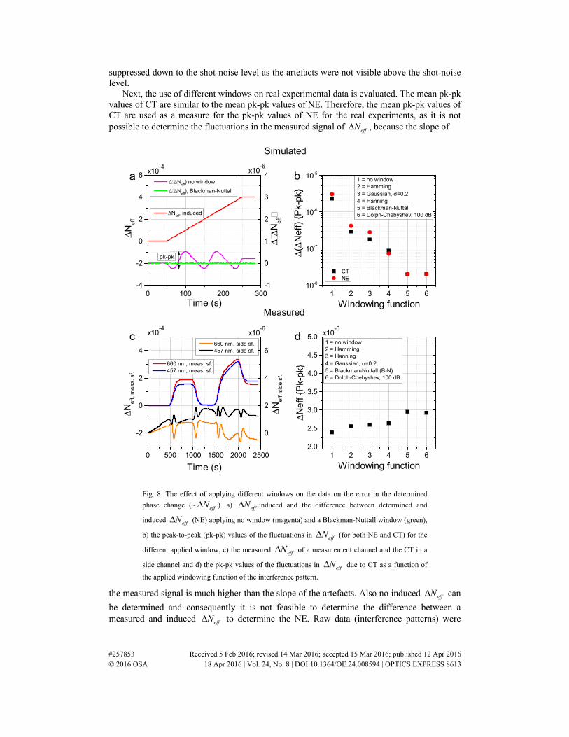
suppressed down to the shot-noise level as the artefacts were not visible above the shot-noise level.

Next, the use of different windows on real experimental data is evaluated. The mean pk-pk values of CT are similar to the mean pk-pk values of NE. Therefore, the mean pk-pk values of CT are used as a measure for the pk-pk values of NE for the real experiments, as it is not possible to determine the fluctuations in the measured signal of effNΔ , because the slope of

0 100 200 300-4

-2

0

2

4

6

1 2 3 4 5 610-8

10-7

10-6

10-5

0 500 1000 1500 2000 2500

-2

0

2

4

1 2 3 4 5 62.0

2.5

3.0

3.5

4.0

4.5

5.0

ΔNe

ff

Time (s)

ΔNeff

, induced

-1

0

1

2

3

4x10-4

Δ ΔNeff

) no window

Δ ΔNeff

), Blackman-Nuttall

x10-6

ΔΔN

eff

pk-pk

CT NE

Δ(ΔN

eff)

{P

k-pk

}Windowing function

1 = no window2 = Hamming 3 = Gaussian, σ=0.24 = Hanning 5 = Blackman-Nuttall 6 = Dolph-Chebyshev, 100 dB

ΔNe

ff,

me

as.

sf.

Time (s)

660 nm, meas. sf. 457 nm, meas. sf.

x10-4

x10-6

0

2

4

6 660 nm, side sf. 457 nm, side sf.

ΔNe

ff,

sid

e s

f.

x10-6

c d

b

Measured

1 = no window2 = Hamming 3 = Hanning 4 = Gaussian, σ=0.25 = Blackman-Nuttall (B-N)6 = Dolph-Chebyshev, 100 dB

ΔNef

f {P

k-pk

}

Windowing function

Simulated

a

Fig. 8. The effect of applying different windows on the data on the error in the determined

phase change (~ effNΔ ). a) effNΔ induced and the difference between determined and

induced effNΔ (NE) applying no window (magenta) and a Blackman-Nuttall window (green),

b) the peak-to-peak (pk-pk) values of the fluctuations in effNΔ (for both NE and CT) for the

different applied window, c) the measured effNΔ of a measurement channel and the CT in a

side channel and d) the pk-pk values of the fluctuations in effNΔ due to CT as a function of

the applied windowing function of the interference pattern.

the measured signal is much higher than the slope of the artefacts. Also no induced effNΔ can

be determined and consequently it is not feasible to determine the difference between a measured and induced effNΔ to determine the NE. Raw data (interference patterns) were


saved and different windows were applied on the measured data. Figure 8(c) shows the fluctuations in effNΔ due to CT for a typical measurement where first D-glucose only

(between t ≈500 and 1000 s) and subsequently D-glucose plus 85 nm beads (between t ≈1500 and 2000 s) were added simultaneously to the sensor. Figure 8(d) shows the pk-pk value of the first artefact in effNΔ (at t ≈500 - 700 s) due to CT as a function of the applied window.

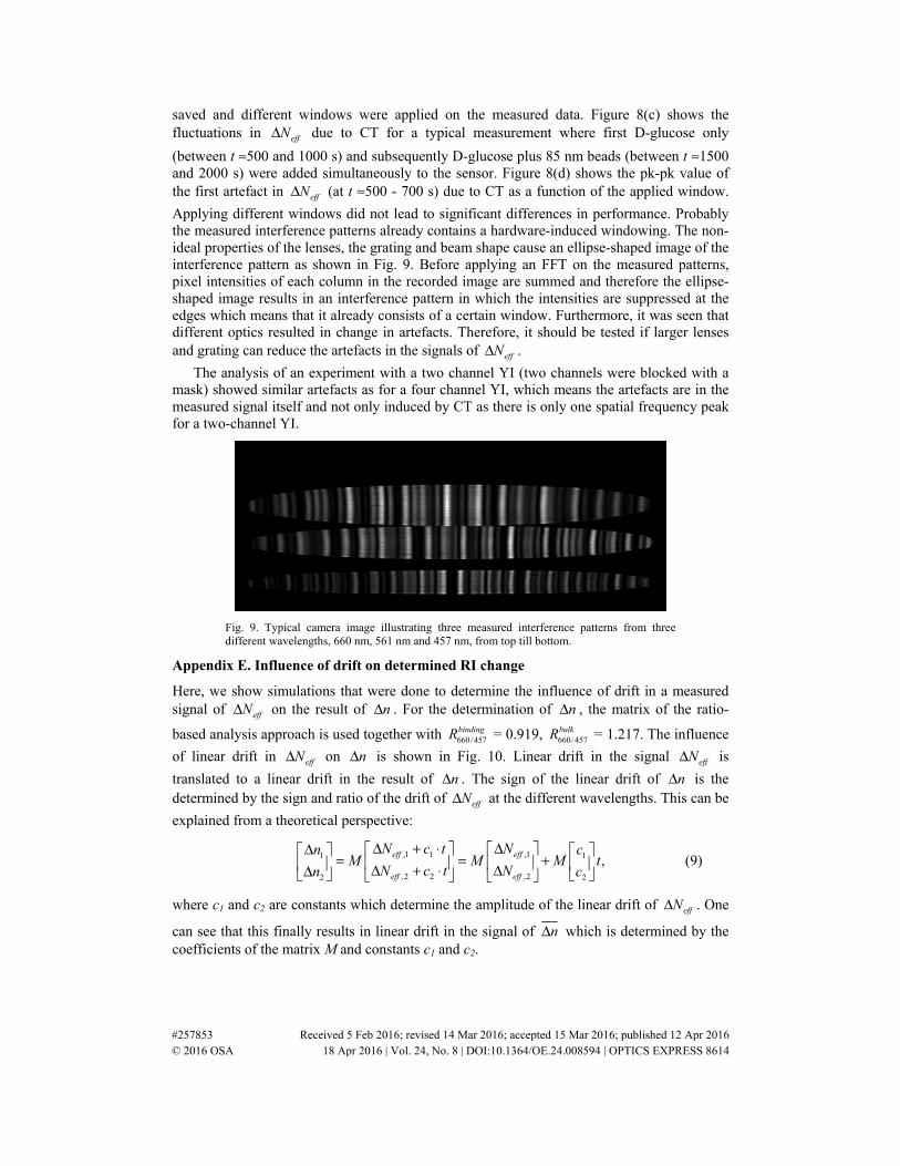
Applying different windows did not lead to significant differences in performance. Probably the measured interference patterns already contains a hardware-induced windowing. The non-ideal properties of the lenses, the grating and beam shape cause an ellipse-shaped image of the interference pattern as shown in Fig. 9. Before applying an FFT on the measured patterns, pixel intensities of each column in the recorded image are summed and therefore the ellipse-shaped image results in an interference pattern in which the intensities are suppressed at the edges which means that it already consists of a certain window. Furthermore, it was seen that different optics resulted in change in artefacts. Therefore, it should be tested if larger lenses and grating can reduce the artefacts in the signals of effNΔ .

The analysis of an experiment with a two channel YI (two channels were blocked with a mask) showed similar artefacts as for a four channel YI, which means the artefacts are in the measured signal itself and not only induced by CT as there is only one spatial frequency peak for a two-channel YI.

Fig. 9. Typical camera image illustrating three measured interference patterns from three different wavelengths, 660 nm, 561 nm and 457 nm, from top till bottom.

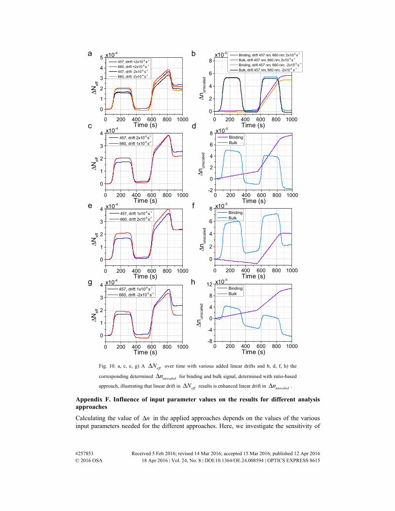
Appendix E. Influence of drift on determined RI change

Here, we show simulations that were done to determine the influence of drift in a measured signal of effNΔ on the result of nΔ . For the determination of nΔ , the matrix of the ratio-

based analysis approach is used together with 660/457bindingR = 0.919, 660/457

bulkR = 1.217. The influence

of linear drift in effNΔ on nΔ is shown in Fig. 10. Linear drift in the signal effNΔ is

translated to a linear drift in the result of nΔ . The sign of the linear drift of nΔ is the determined by the sign and ratio of the drift of effNΔ at the different wavelengths. This can be

explained from a theoretical perspective:

,1 1 ,11 1

,2 2 ,22 2

,eff eff

eff eff

N c t Nn cM M M t

N c t Nn c

Δ + ⋅ ΔΔ = = + Δ + ⋅ ΔΔ

(9)

where c1 and c2 are constants which determine the amplitude of the linear drift of effNΔ . One

can see that this finally results in linear drift in the signal of nΔ which is determined by the coefficients of the matrix M and constants c1 and c2.


0 200 400 600 800 1000

0

1

2

3

4

5

0 200 400 600 800 1000

0

2

4

6

8

0 200 400 600 800 1000

0

1

2

3

4

0 200 400 600 800 1000-2

0

2

4

6

8

0 200 400 600 800 1000

0

1

2

3

4

0 200 400 600 800 1000

0

2

4

6

8

0 200 400 600 800 1000

0

1

2

3

4

0 200 400 600 800 1000-8

-4

0

4

8

12

x10-4

ΔNe

ff

Time (s)

457, ldrift +2x10-8 s-1

660, drift +2x10-8 s-1

457, drift -2x10-8 s-1

660, drift -2x10-8 s-1

x10-5

Δnu

nsc

ale

d

Time (s)

Binding, drift 457 nm, 660 nm: 2x10-8 s-1

Bulk, drift 457 nm, 660 nm: 2x10-8 s-1

Binding, drift 457 nm, 660 nm: -2x10-8 s-1

Bulk, drift 457 nm, 660 nm: -2x10-8 s-1

x10-4

ΔNe

ff

Time (s)

457, drift 2x10-8 s-1

660, drift 1x10-8 s-1

x10-5

Δnu

nsc

ale

dTime (s)

Binding Bulk

e

g h

f

d

b

c

x10-4

ΔNe

ff

Time (s)

457, drift 1x10-8 s-1

660, drift 2x10-8 s-1

a

x10-5Δn

un

sca

led

Time (s)

Binding Bulk

x10-4

ΔNe

ff

Time (s)

457, drift 1x10-8 s-1

660, drift -2x10-8 s-1

Δnu

nsc

ale

d

Time (s)

Binding Bulk

x10-5

Fig. 10. a, c, e, g) A effNΔ over time with various added linear drifts and b, d, f, h) the

corresponding determined unscalednΔ for binding and bulk signal, determined with ratio-based

approach, illustrating that linear drift in effNΔ results is enhanced linear drift in unscalednΔ .

Appendix F. Influence of input parameter values on the results for different analysis approaches

Calculating the value of nΔ in the applied approaches depends on the values of the various input parameters needed for the different approaches. Here, we investigate the sensitivity of


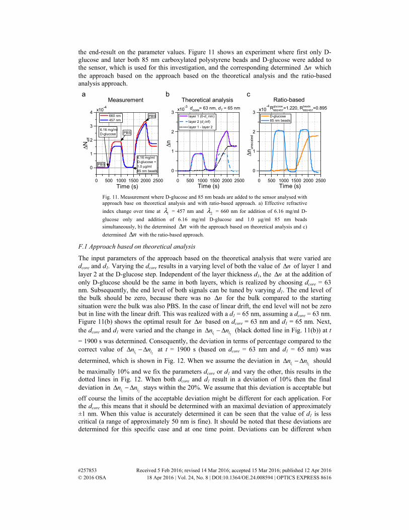
the end-result on the parameter values. Figure 11 shows an experiment where first only D-glucose and later both 85 nm carboxylated polystyrene beads and D-glucose were added to the sensor, which is used for this investigation, and the corresponding determined nΔ which the approach based on the approach based on the theoretical analysis and the ratio-based analysis approach.

0 500 1000 1500 2000 2500

0

1

2

3

4

0 500 1000 1500 2000 2500

0

1

2

3

0 500 1000 1500 2000 2500

0

1

2

3

PBS6.16 mg/ml D-glucose

ΔNe

ff

Time (s)

660 nm 457 nm

x10-4

PBS

PBS

6.16 mg/ml D-glucose +1.0 μg/ml 85 nm beads

Δn

Time (s)

layer 1 (0-d1 nm)

layer 2 (d1-inf)

layer 1 - layer 2

x10-3 dcore= 63 nm, d1 = 65 nm

cbRatio-basedTheoretical analysis

x10-4

Δnu

nsca

led

Time (s)

D-glucose 85 nm beads

Rglucose

660/457=1.220, Rbeads

660/457=0.895

Measurementa

Fig. 11. Measurement where D-glucose and 85 nm beads are added to the sensor analysed with approach base on theoretical analysis and with ratio-based approach. a) Effective refractive

index change over time at 1λ = 457 nm and 2λ = 660 nm for addition of 6.16 mg/ml D-

glucose only and addition of 6.16 mg/ml D-glucose and 1.0 μg/ml 85 nm beads simultaneously, b) the determined nΔ with the approach based on theoretical analysis and c)

determined nΔ with the ratio-based approach.

F.1 Approach based on theoretical analysis

The input parameters of the approach based on the theoretical analysis that were varied are dcore and d1. Varying the dcore results in a varying level of both the value of nΔ of layer 1 and layer 2 at the D-glucose step. Independent of the layer thickness d1, the nΔ at the addition of only D-glucose should be the same in both layers, which is realized by choosing dcore = 63 nm. Subsequently, the end level of both signals can be tuned by varying d1. The end level of the bulk should be zero, because there was no nΔ for the bulk compared to the starting situation were the bulk was also PBS. In the case of linear drift, the end level will not be zero but in line with the linear drift. This was realized with a d1 = 65 nm, assuming a dcore = 63 nm. Figure 11(b) shows the optimal result for nΔ based on dcore = 63 nm and d1 = 65 nm. Next, the dcore and d1 were varied and the change in

1 2l ln nΔ − Δ (black dotted line in Fig. 11(b)) at t

= 1900 s was determined. Consequently, the deviation in terms of percentage compared to the correct value of

1 2l ln nΔ − Δ at t = 1900 s (based on dcore = 63 nm and d1 = 65 nm) was

determined, which is shown in Fig. 12. When we assume the deviation in 1 2l ln nΔ − Δ should

be maximally 10% and we fix the parameters dcore or d1 and vary the other, this results in the dotted lines in Fig. 12. When both dcore and d1 result in a deviation of 10% then the final deviation in

1 2l ln nΔ − Δ stays within the 20%. We assume that this deviation is acceptable but

off course the limits of the acceptable deviation might be different for each application. For the dcore this means that it should be determined with an maximal deviation of approximately ±1 nm. When this value is accurately determined it can be seen that the value of d1 is less critical (a range of approximately 50 nm is fine). It should be noted that these deviations are determined for this specific case and at one time point. Deviations can be different when


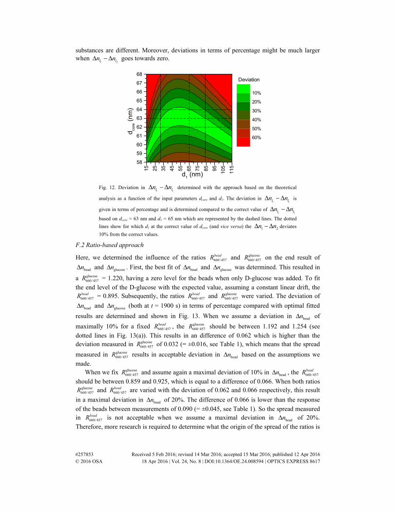
substances are different. Moreover, deviations in terms of percentage might be much larger when

1 2l ln nΔ − Δ goes towards zero.

15 25 35 45 55 65 75 85 95 105

115

58

59

60

61

62

63

64

65

66

67

68Deviation

d1 (nm)

d core (

nm)

10%

20%

30%

40%

50%

60%

Fig. 12. Deviation in 1 1l ln nΔ − Δ determined with the approach based on the theoretical

analysis as a function of the input parameters dcore and d1. The deviation in 1 1l ln nΔ − Δ is

given in terms of percentage and is determined compared to the correct value of 1 1l ln nΔ − Δ

based on dcore = 63 nm and d1 = 65 nm which are represented by the dashed lines. The dotted

lines show for which d1 at the correct value of dcore (and vice versa) the 1 2n nΔ − Δ deviates

10% from the correct values.

F.2 Ratio-based approach

Here, we determined the influence of the ratios 660/457beadR and glucose

660/457R on the end result of

beadnΔ and glucosenΔ . First, the best fit of beadnΔ and glucosenΔ was determined. This resulted in

a glucose660/457R = 1.220, having a zero level for the beads when only D-glucose was added. To fit

the end level of the D-glucose with the expected value, assuming a constant linear drift, the

660/457beadR = 0.895. Subsequently, the ratios 660/457

beadR and glucose660/457R were varied. The deviation of

beadnΔ and glucosenΔ (both at t = 1900 s) in terms of percentage compared with optimal fitted

results are determined and shown in Fig. 13. When we assume a deviation in beadnΔ of

maximally 10% for a fixed 660/457beadR , the glucose

660/457R should be between 1.192 and 1.254 (see

dotted lines in Fig. 13(a)). This results in an difference of 0.062 which is higher than the deviation measured in glucose

660/457R of 0.032 (= ±0.016, see Table 1), which means that the spread

measured in glucose660/457R results in acceptable deviation in beadnΔ based on the assumptions we

made. When we fix glucose

660/457R and assume again a maximal deviation of 10% in beadnΔ , the 660/457beadR

should be between 0.859 and 0.925, which is equal to a difference of 0.066. When both ratios glucose660/457R and 660/457

beadR are varied with the deviation of 0.062 and 0.066 respectively, this result

in a maximal deviation in beadnΔ of 20%. The difference of 0.066 is lower than the response

of the beads between measurements of 0.090 (= ±0.045, see Table 1). So the spread measured in 660/457

beadR is not acceptable when we assume a maximal deviation in beadnΔ of 20%.

Therefore, more research is required to determine what the origin of the spread of the ratios is


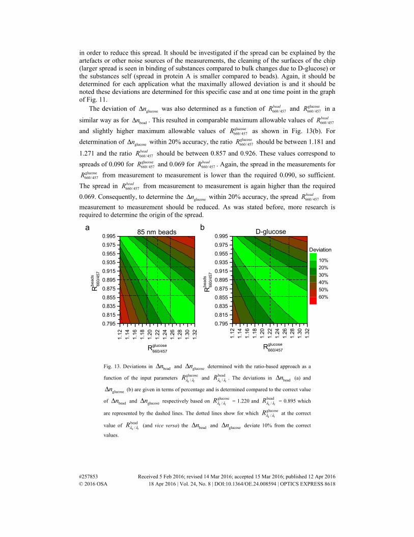
in order to reduce this spread. It should be investigated if the spread can be explained by the artefacts or other noise sources of the measurements, the cleaning of the surfaces of the chip (larger spread is seen in binding of substances compared to bulk changes due to D-glucose) or the substances self (spread in protein A is smaller compared to beads). Again, it should be determined for each application what the maximally allowed deviation is and it should be noted these deviations are determined for this specific case and at one time point in the graph of Fig. 11.

The deviation of glucosenΔ was also determined as a function of 660/457beadR and glucose

660/457R in a

similar way as for beadnΔ . This resulted in comparable maximum allowable values of 660/457beadR

and slightly higher maximum allowable values of glucose660/457R as shown in Fig. 13(b). For

determination of glucosenΔ within 20% accuracy, the ratio glucose660/457R should be between 1.181 and

1.271 and the ratio 660/457beadR should be between 0.857 and 0.926. These values correspond to

spreads of 0.090 for glucose660/457R and 0.069 for 660/457

beadR . Again, the spread in the measurements for glucose660/457R from measurement to measurement is lower than the required 0.090, so sufficient.

The spread in 660/457beadR from measurement to measurement is again higher than the required

0.069. Consequently, to determine the glucosenΔ within 20% accuracy, the spread 660/457beadR from

measurement to measurement should be reduced. As was stated before, more research is required to determine the origin of the spread.

1.12

1.14

1.16

1.18

1.20

1.22

1.24

1.26

1.28

1.30

1.32

0.795

0.815

0.835

0.855

0.875

0.895

0.915

0.935

0.955

0.975

0.995

Deviation

85 nm beads

Rglucose

660/457

Rb

ea

ds

66

0/4

57

1.12

1.14

1.16

1.18

1.20

1.22

1.24

1.26

1.28

1.30

1.32

0.795

0.815

0.835

0.855

0.875

0.895

0.915

0.935

0.955

0.975

0.995

bD-glucose

Rglucose

660/457

Rb

ea

ds

66

0/4

57

10%

20%

30%

40%

50%

60%

a

Fig. 13. Deviations in beadnΔ and glucosenΔ determined with the ratio-based approach as a

function of the input parameters glucose

/k lRλ λ and

bead/k l

Rλ λ . The deviations in beadnΔ (a) and

glucosenΔ (b) are given in terms of percentage and is determined compared to the correct value

of beadnΔ and glucosenΔ respectively based on glucose

/k lRλ λ = 1.220 and

bead/k l

Rλ λ = 0.895 which

are represented by the dashed lines. The dotted lines show for which glucose

/k lRλ λ at the correct

value of bead

/k lRλ λ (and vice versa) the beadnΔ and glucosenΔ deviate 10% from the correct

values.


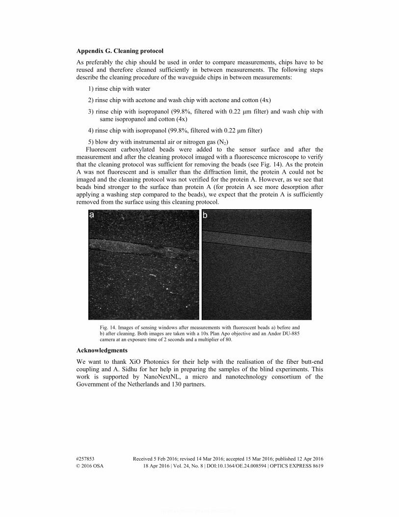
Appendix G. Cleaning protocol

As preferably the chip should be used in order to compare measurements, chips have to be reused and therefore cleaned sufficiently in between measurements. The following steps describe the cleaning procedure of the waveguide chips in between measurements:

1) rinse chip with water

2) rinse chip with acetone and wash chip with acetone and cotton (4x)

3) rinse chip with isopropanol (99.8%, filtered with 0.22 μm filter) and wash chip with same isopropanol and cotton (4x)

4) rinse chip with isopropanol (99.8%, filtered with 0.22 μm filter)

5) blow dry with instrumental air or nitrogen gas (N2) Fluorescent carboxylated beads were added to the sensor surface and after the

measurement and after the cleaning protocol imaged with a fluorescence microscope to verify that the cleaning protocol was sufficient for removing the beads (see Fig. 14). As the protein A was not fluorescent and is smaller than the diffraction limit, the protein A could not be imaged and the cleaning protocol was not verified for the protein A. However, as we see that beads bind stronger to the surface than protein A (for protein A see more desorption after applying a washing step compared to the beads), we expect that the protein A is sufficiently removed from the surface using this cleaning protocol.

Fig. 14. Images of sensing windows after measurements with fluorescent beads a) before and b) after cleaning. Both images are taken with a 10x Plan Apo objective and an Andor DU-885 camera at an exposure time of 2 seconds and a multiplier of 80.

Acknowledgments

We want to thank XiO Photonics for their help with the realisation of the fiber butt-end coupling and A. Sidhu for her help in preparing the samples of the blind experiments. This work is supported by NanoNextNL, a micro and nanotechnology consortium of the Government of the Netherlands and 130 partners.


Documents

Size-selective analyte detection with a Young ... fileSize-selective analyte detection with a Young interferometer sensor using multiple wavelengths Harmen K. P. Mulder,1,* Christian