This book is an introduction to geometric representation theory.1

What is geometric representation theory? It is hard to define exactly2

what it is as this subject is constantly growing in methods and scope.3

The main aim of this area is to approach representation theory which4

deals with symmetry and non-commutative structures by geometric5

methods (and also get insights on the geometry from the representa-6

tion theory). Here by geometry we mean any local to global situation7

where one tries to understand complicated global structures by gluing8

them from simple local structures. The main example is the Beilinson-9

Bernstein localization theorem. This theorem essentially says that the10

representation theory of a semi-simple Lie algebra (such as sl(n,C)) is11

encoded in the geometry of its flag variety. This theorem enables the12

transfer of “hard” (global) problems about the universal enveloping al-13

gebra, to “easy” (local) problems in geometry. The Beilinson-Bernstein14

localization theorem has been extremely useful in solving problems in15

representation theory of semi-simple Lie algebras and in gaining deeper16

insight into the structure of representation theory as a whole. There17

are many more examples of geometric representation theory in action,18

from Deligne-Lusztig varieties to the geometric Langlands’ program19

and categorification.20

The focus of this book is the Beilinson-Bernstein localization theo-21

rem. It follows the advice of the great mathematician Israel M. Gelfand:22

we only cover the case of sl2 (classical and quantum). This approach23

allows us to introduce many topics in a very concrete way without go-24

ing into the general theory. Thus we cover the Peter-Weyl theorem,25

the Borel-Weil theorem, the Beilinson-Bernstein theorem and much26

more for both the classical and quantum case. Dealing with the quan-27

tum case allows us also to introduce many tools from non-commutative28

algebraic geometry and quantum groups. These topics are usually con-29

sidered very advanced. To have a full understanding of them requires30

a good grasp of algebraic geometry, D-module theory, category theory,31

homological algebra and the theory of semi-simple Lie algebras. We32

think that by focusing on the simplest case of sl2 the student can gain33

much insight and intuition into the subject. A good and deep under-34

standing of sl2 makes the general theory much simpler to learn and35

appreciate.36

This book is based on a graduate lecture course given at MIT by37

the second author. We are grateful to the students taking that course38

for sharing their notes with us as we prepared this manuscript.39

i

Contents40

Introduction 141

Chapter 1. The first classical example: sl2. 242

1. The Lie algebra sl2 343

2. Irreducible finite-dimensional modules 444

3. The universal enveloping algebra 545

4. Semisimplicity 646

5. Characters 847

6. The PBW theorem, and the center of U(sl2) 948

Chapter 2. Hopf algebras and tensor categories 1249

1. Hopf algebras 1350

2. The first examples of Hopf Algebras 1651

2.1. The Hopf algebra U(sl2) 1652

2.2. The Hopf algebra O(SL2) 1653

3. Tensor Categories 1754

Chapter 3. Geometric Representation Theory for SL2 2055

1. The algebra of matrix coefficients 2156

2. Peter-Weyl Theorem for SL(2) 2257

3. Reconstructing O(SL2) from U(sl2) via matrix coefficients. 2358

4. Equivariant vector bundles, and sheaves 2459

5. Quasi-coherent sheaves on the flag variety 2660

6. The Borel-Weil Theorem 2861

7. Beilinson-Bernstein Localization 3062

7.1. D-modules on P1 3063

7.2. The Localization Theorem 3164

Chapter 4. The first quantum example: Uq(sl2). 3465

1. The quantum integers 3566

2. The quantum enveloping algebra Uq(sl2) 3567

3. Representation theory for Uq(sl2) 3768

4. Uq is a Hopf algebra 3869

5. More representation theory for Uq 3970

5.1. Quantum Casimir element 4071

ii

CONTENTS iii

6. The locally finite part and the center of Uq(sl2) 4172

Chapter 5. Categorical Commutativity in Braided Tensor73

Categories 4374

1. Braided and Symmetric Tensor Categories 4475

2. R-matrix Preliminaries 4676

3. Drinfeld’s Universal R-matrix 4777

4. Lusztig’s R-matrices 4778

5. Weights of Type I, and bicharacters (needs better title) 4879

6. The Yang-Baxter Equation 5080

7. The hexagon Diagrams 5381

Chapter 6. Geometric Representation Theory for SLq(2) 5482

1. The Quantum Group Algebra 5583

2. Generators and Relations for Oq 5584

3. Oq comodules 5785

4. Borel-Weil Correspondences in Classical and Quantum86

Cases 5887

4.1. The Quantum case 5988

4.2. An equivalence of categories arising from the Hopf pairing 6089

4.3. Restriction and Induction Functors 6190

4.4. Quantum P1 6291

5. Lecture 14 - Quasi-coherent sheaves 6492

5.1. Classical case 6493

5.2. Quantum case 6694

5.3. Quantum differential operators on A2q 6895

6. Quantum D-modules 7096

Bibliography 7597

INTRODUCTION 1

Introduction98

In representation theory, the Lie algebra sl2 := sl2(C) comprises the99

first and most important example of a semi-simple Lie algebra. In this100

introductory text, which grew out of a course taught by the first au-101

thor, we will walk the reader through important concepts in geometric102

representation theory, as well as their quantum group analogues. Our103

focus is on developing concrete examples to illustrate the geometric104

notions discussed in the text. As such, we will restrict our attention105

almost exclusively to sl2, giving more general definitions only when it106

is convenient or illustrative.107

In Chapter 1, we show that the category of finite-dimensional sl2-108

modules is a semi-simple abelian category; we prove this important fact109

in a way which will generalize most easily to the quantum setting in110

later chapters.111

In Chapter 2, we introduce the formalisms of Hopf algebras and112

tensor categories. These capture the essential properties of algebraic113

groups, their representations, and their coordinate algebras, in a way114

that can be extended to the quantum setting.115

In Chapter 3, we discuss the relation between geometry of various116

G-varieties and the representation theory of G. We discuss the Peter-117

Weyl theorem, and obtain as a corollary the Borel-Weil theorem. We118

define D-modules on P1, and we relate them to representations of sl2:119

this is the first instance of the so-called Beilinson-Bernstein localization120

theorem.121

In Chapter 4, we introduce the quantized universal enveloping al-122

gebra Uq(sl2), and extend the results of Chapter 1 to the quantum123

setting.124

In Chapter 5, we explain the notion of a braided tensor category,125

a mild generalization of the notion of a symmetric tensor category.126

Braided tensor categories underlie the representation theory of Uq(sl2)127

in a way analogous to the role of symmetric tensor categories in the128

representation theory of sl2.129

In Chapter 6, we reproduce the results of Chapter 3 in the quantum130

setting. We have quantum analogs of each of the Peter-Weyl, Borel-131

Weil, and Beilinson-Bernstein theorems.132

Throughout the text assume some passing familiarity with the the-133

ory of Lie algebras. Two excellent introductions are Humphreys [?]134

and Knapp [?].135

CHAPTER 1

The first classical example: sl2.136

2

1. THE LIE ALGEBRA sl2 3

1. The Lie algebra sl2137

The Lie algebra sl2 := sl2(C) consists of the traceless 2×2 matrices,with the standard Lie bracket:

[A,B] := AB − BA.

A standard and convenient presentation of sl2(C) is given as follows.138

We let:139

(1) E =

�0 10 0

�, F =

�0 01 0

�, H =

�1 00 −1

�,

Then sl2 is spanned by E,F , and H, with commutators:

[H,E] = 2E, [H,F ] = −2F, [E,F ] = H.

Recall that a representation of g (equivalently, a g-module) is a vec-140

tor space V , together with a Lie algebra homomorphism ρ : g→ End(V ).141

We will often omit ρ from notation, and write simply x.v for ρ(x).v.142

The finite-dimensional representations of sl2 are sufficiently compli-143

cated to be interesting, yet can be completely understood by elemen-144

tary means. In this chapter, we recall their classification. We begin145

with some examples:146

Example 1.1. The defining representation. The Lie algebra sl2147

acts on C2 by matrix multiplication.148

Example 1.2. The adjoint representation. Any Lie algebra g acts149

on itself by x.y := [x, y].150

Example 1.3. Given any representation V of a Lie algebra g, its151

dual vector space V ∗ carries an action defined by (X.f)(v) = f(−X.v).152

The corresponding representation is also denoted V ∗.153

Example 1.4. Given two representations V and W of g, the vector154

space V ⊕W carries an action of g defined by x(v, w) := (xv, xw) for155

(v, w) ∈ V ⊕W , and x ∈ g. The corresponding representation is also156

denoted V ⊕W .157

Example 1.5. Given two representations V and W , the vector158

space V ⊗ W carries an action of g defined by x(v ⊗ w) = x(v) ⊗159

w + v ⊗ x(w), for v ⊗ w ∈ V ⊗ W , and x ∈ g. The corresponding160

representation is also denoted V ⊗W .161

As we will see in Chapter 2, these examples make the category of162

g-modules into an abelian tensor category with duals (see also [?]).163

2. IRREDUCIBLE FINITE-DIMENSIONAL MODULES 4

2. Irreducible finite-dimensional modules164

Definition 2.1. Let V be an sl2-module. A non-zero v ∈ V is165

a weight vector of weight λ if Hv = λv. A highest weight vector is a166

weight vector v of V such that Ev = 0. Denote by Vλ the subspace of167

weight vectors of weight λ.168

Observe that commutation relations (1) imply EVλ ⊂ Vλ+2, and169

FVλ ⊂ Vλ−2.170

Exercise 2.2. Prove that every finite dimensional sl2 module has171

a highest weight vector.172

It follows that any irreducible finite dimensional representation is173

generated by a highest weight vector; this fact will be the key to their174

classification.175

Lemma 2.3. Let V be a finite-dimensinal sl2-module, and suppose176

there exists a highest weight vector v0, of weight λ. Let vi := (1/i!)F i(v0)177

(by convention, v−1 = 0). Then we have that:178

(2) Hvi = (λ− 2i)vi, Fvi = (i + 1)vi+1, Evi = (λ− i + 1)vi−1.

Proof. The first two relations are obvious, and the third is a179

straightforward computation:180

iEvi = EFvi−1 = [E,F ]vi−1 + FEvi−1

= Hvi−1 + FEvi−1 = (λ− 2i + 2)vi−1 + (λ− i + 2)Fvi−2

= (λ− 2i + 2)vi−1 + (i− 1)(λ− i + 2)vi−1 = i(λ− i + 1)vi−1.

�181

Theorem 2.4. Let V be an irreducible finite dimensional sl2-module.182

Then V has a unique (up to scalar) highest weight vector of weight183

m := dimV − 1. Further, V decomposes as a direct sum of one dimen-184

sional weight spaces of weights m,m− 2, . . . , 2−m,−m.185

Proof. It follows from Lemma 2.3 that span{vi}i∈N is a submodule186

of V , and thus all of V . We let m ≥ 0 be maximal such that vm �=187

0 (equivalently, vm+1 is the first which is zero). Then by the third188

equation of equation (2): 0 = Evm+1 = (λ − m)vm. Therefore we189

see that λ = m, and that dimV = m + 1. Further, it is immediate190

that the three formulas (with λ = m) define a representation of sl2191

on a vector space of dimension m + 1, which we will denote V (m).192

Any such representation is irreducible, as applying E to a vector w193

repeatedly will eventually yield a nonzero multiple of v0, and thus w194

generates all of V . �195

3. THE UNIVERSAL ENVELOPING ALGEBRA 5

We note three important examples: firstly, the trivial representation196

is the weight zero irreducible. The defining representation of sl2 on 2-197

space is the weight one irreducible. Finally, we note that the adjoint198

representation is three dimensional of highest weight 2, and this implies199

that sl2 is a simple Lie algebra.200

3. The universal enveloping algebra201

The universal enveloping algebra U(g), of a Lie algebra g, is thequotient of the free associative algebra on the vector space g (i.e. thetensor algebra T (g)), by the commutator relations a⊗ b− b⊗a = [a, b].That is,

U(g) := T (g)/�a⊗ b− b⊗ a− [a, b]�.The canonical inclusion g �→ T (V ) induces a natural map i : g →202

U(g). This gives rise to a functor U from Lie algebras to associative203

algebras. We also have a forgetful functor F from associative algebras204

to Lie algebras, given by defining [a, b] := ab− ba, and then forgetting205

the associative multiplication.206

Remark 3.1. Actually, the PBW theorem implies that the map207

i : g→ U(g) is an inclusion, but this is not needed in what follows.208

Proposition 3.2. The functors (U, F ) form an adjoint pair.209

Proof. We need an isomorphism φ : Hom(U(g), A)→ Hom(g, F (A)).210

Given f : U(g) → A, we define φ(f) = f ◦ i. It is easy to check that211

this gives the required isomorphism. �212

By the adjointness above,a g-module is the same as an associative213

algebra homomorphism ρ : U(g) → End(V ). In other words, we have214

an equivalence of categories g-Mod ∼ U(g)-Mod. Thus we may view215

representation theory of Lie algebras as a sub-branch of representation216

theory of associative algebras, rather than something entirely new.217

The universal enveloping algebra of sl2 contains an important cen-218

tral element, which will feature in the next section.219

Definition 3.3. The Casimir element, C ∈ U(sl2), is given by theformula:

C = EF + FE +H2

2.

Claim 3.4. C is a central element of U(sl2).220

4. SEMISIMPLICITY 6

Proof. It suffices to show that C commutes with the generatorsE,F,H. We compute:

[E,C] = [E,EF ] + [E,FE] + [E,H2

2]

= [E,E]F + E[E,F ] + [E,F ]E + F [E,E]

+1

2([E,H]H + H[E,H])

= EH + HE − EH −HE = 0.

The bracket [C, F ] is zero by a similar computation or by consideration221

of the automorphism switching E and F and taking H to −H.222

Taking the bracket with H gives:

[H,C] = [H,E]F + E[H,F ] + [H,F ]E + F [H,E]

= 2EF − 2EF − 2FE + 2FE = 0,

which proves the claim. �223

4. Semisimplicity224

Having classified irreducible finite dimensional representations, we225

now wish to extend this classification to all finite dimensional repre-226

sentations. This is accomplished by the following:227

Theorem 4.1. The category of finite dimensional sl2-modules is228

semisimple: any finite dimensional sl2-module is projective and thus229

decomposes as a direct sum of simples.230

In the proof of the theorem, we will use the following characteriza-231

tion of semi-simplicity:232

Exercise 4.2. Show that an abelian category is semi-simple if, and233

only if, for every object X the functor Hom(X,−) is projective. Hint:234

for the “if” direction, consider an exact sequence 0→ U → V → W →235

0, and apply the functor Hom(W,−) to produce the required splitting236

W → V .237

By the exercise, we need to show that, for any finite dimensionalsl2-module X, the functor Homsl2(X,−) is exact on finite dimensionalmodules. We have a natural isomorphism,

φ : Homsl2(V,W∗ ⊗ L)

∼→ Homsl2(V ⊗W,L).

f �→ φ(f),

4. SEMISIMPLICITY 7

where φ(f)(v⊗w) := �f(v), w�. Let I denote the trivial representation;we have a natural isomorphism, X ∼= I ⊗X, for any X. Therefore wehave natural isomorphisms:

Homsl2(X, V ) ∼= Homsl(2)(I ⊗X, V ) ∼= Homsl2(I,X∗ ⊗ V ).

As these are all vector spaces, tensoring by X∗ is an exact functor. So238

we see that to prove the claim it suffices to show that Homsl2(I,−) is239

exact.240

A homomorphism from the trivial module into V is simply the241

choice of a vector v with the property that xv = 0 for all x ∈ sl2. The242

set of all such v is a submodule of V , denoted V sl2 , which is naturally243

isomorphic to Homsl2(I, V ). So we have reduced the above theorem244

to:245

Lemma 4.3. For any finite dimensional sl2-module V , the functor246

V → V sl2 is an exact functor.247

The proof of this lemma will rely upon the central Casimir element248

C ∈ U(sl2). Note that, by Schur’s lemma C will act as a scalar on any249

finite dimensional irreducible V .250

Exercise 4.4. If V is irreducible of highest weight m, then C acts251

as scalar multiplication by m2+2m2

(hint: it suffices to compute the252

action of C on a highest-weight vector).253

Proposition 4.5. Let V a finite dimensional sl2 module. If Ck254

acts as 0 on V for some k > 0, then sl2 acts trivially on V .255

Proof. We proceed by induction on dimV , the case dimV = 0256

being trivial. Let U ⊂ V be a maximal proper submodule (U = 0257

is possible). By induction, sl2U = 0. Further, V/U is an irreducible258

module, and by the above we know that C acts as a nonzero scalar259

(and hence so does Ck) on V/U unless V/U is the trivial 1 dimensional260

module. Thus, for v ∈ V , xv ∈ U for all x ∈ sl2 and so yxv = 0261

for all y ∈ sl2. Therefore [x, y]v = 0; however, since sl2 is a simple262

Lie algebra, we have [sl2, sl2] = sl2, and thus V is a trivial module as263

required. �264

Remark 4.6. [?], [?] The Casimir element C may defined for any265

finite dimensional semi-simple Lie algebra, using the Killing form. It266

can be shown that this is a central element which acts nontrivially on267

nonzero irreducible modules.268

Now, the following proposition finishes the argument:269

Proposition 4.7. Let V a finite dimensional sl2 module. Then270

5. CHARACTERS 8

(1) ker(C) = V sl2.271

(2) ker(C2) ⊆ ker(C).272

(3) V = ker(C)⊕ im(C).273

(4) The functor V �→ V sl2 is exact.274

Proof. Claim (1) is immediate from Exercise 4.4 above; togetherwith Proposition 4.5, it implies (2). We have ker(C) ∩ im(C) = 0,by Claim (2), which implies (3). To see (4), we first construct achain complex V = 0 → V → V → 0, where the middle differen-tial is multiplication by C (a morphism because C is central). We haveH1(V ) = H0(V ) ∼= V sl2 by (2). Suppose we have an exact sequenceof sl2-modules 0 → U → V → W → 0. Since C ∈ U(sl2), the mapsnecessarily commute with the differentials to give an exact sequence ofthe complexes:

0→ Ui→ V

j→ W → 0.

We apply the snake lemma to obtain the long exact sequence,

0→ U0i1−→ V sl2 j1−→ W sl2 δ−→ U sl2 i0−→ V sl2 j0−→ W sl2 → 0.

Further, the induced map i0 : U sl2 → V sl2 may be identified with275

the restriction of the original map U → W . By assumption this was276

injective, and so im(δ) = 0 and the induced right-hand sequence of277

invariants is exact as required. �278

Remark 4.8. The above proof can be slightly modified to apply to279

a general semi-simple Lie algebra with Casimir element C.280

While Proposition 4.7 guarantees that a general V can be split into281

a direct sum of simple sl2 modules, the following is a more explicit282

algorithm for constructing the decomposition.283

(1) Decompose V = ⊕V(m), where V(m) denotes the eigenspace for284

the operator C with eignevalue m2 + 2m285

(2) Within each V(m), choose a basis {vi}ki=1 for the λ = m-weight286

space.287

(3) Set V(m),i = sl2vi, which will be an m dimensional space by288

our characterization above.289

(4) Then V = ⊕m(⊕iV(m),i) is a decomposition into simple mod-290

ules.291

5. Characters292

The representation theory of sl2 admits a powerful theory of char-293

acters, analogous to that of finite groups. Computing characters allows294

us to easily determine the isomorphism type of any finite-dimensional295

sl2-module, and to decompose tensor products.296

6. THE PBW THEOREM, AND THE CENTER OF U(sl2) 9

Definition 5.1. For a finite dimensional sl2 module V , we define297

the formal sum:298

ch(V ) =�

k∈Z(dimVk)x

k,

where we recall that Vk denotes the weight space,

Vk = {v ∈ V |Hv = kv}.Exercise 5.2. Defining xk · xl = xk+l, we have:

ch(A⊕ B) = ch(A) + ch(B), ch(A⊗ B) = ch(A)ch(B).

Example 5.3. By Theorem 2.4, we have:

ch(V (n)) =xn+1 − x−n−1

x− x−1= xn + xn−2 + · · ·+ x2−n + x−n.

Remark 5.4. Suppose V is a finite-dimensional sl2-module,with299

character ch(V ). Then p(x) = ch(V )·(x−x−1) is a Laurent polynomial300

in x. The coefficient of xk in p(x) is the multiplicity of the irrreducible301

V (k) in V .302

Exercise 5.5. (Clebsch-Gordan) Give a decomposition of V (m)⊗303

V (n) as a sum of irreducibles V (i) in two different ways:304

(1) by finding all the highest weight vectors in the tensor product.305

(2) by computing the character.306

Exercise 5.6. Show that the subspace Symn(V (1)) of V (1)⊗n,307

consisting of symmetric tensors, is a sub-module for the sl2 action, and308

is isomorphic to V (n).309

The exercise implies that, as a tensor category, the category of310

sl2-modules is generated by the object V (1): in other words, every311

irreducible sl2-module can be found in some tensor power of V (1).312

Exercise 5.7. Show that V (1)⊗ V (1) ∼= V (2)⊕ V (0).313

We will see in next chapter that this is in some sense the only314

relation in this category.315

6. The PBW theorem, and the center of U(sl2)316

The Poincare-Birkhoff-Witt theorem gives a basis of U(g) for any317

Lie algebra g. The proof we present hinges on a technical result in318

non-commutative algebra known as the diamond lemma, which is of319

independent interest.320

Let k�X� denote the free algebra on a finite set X. Fix a total321

ordering < on X, extend lexicographically to all monomials of the same322

degree, and finally declare m < n, if m is of lesser degree. Further, fix323

6. THE PBW THEOREM, AND THE CENTER OF U(sl2) 10

a finite set S of pairs (mi, fi), of a monomial mi in k�X�, and a general324

element fi ∈ k�X� all of whose monomials are less than mi, or of smaller325

degree. A general monomial in k�X� is called a PBW monomial if it326

contains no mi as a subword. A general element of k�X� is called327

PBW-ordered if it is a sum of PBW monomials.328

Lemma 6.1 (Diamond lemma, [?]). Suppose that:329

(1) “Overlap ambiguities are resolvable”: For every triple of mono-330

mials A,B,C, with some mi = AB, and mj = BC, the expres-331

sions fiC and Afj can be further resolved to the same PBW-332

ordered expression.333

(2) “Inclusion ambiguities are resolvable”: For every A,B,C, with334

mi = B, and mj = ABC, the expressions AfiC and fj can be335

further resolved to the same PBW-ordered expression.336

Then, the set of PBW monomials in k�X� forms a basis for the quotient337

ring k�X�/�mi − fi|(mi, fi) ∈ S�.338

The defining relations of U(sl2) fit into the above formalism, withE < H < F and:

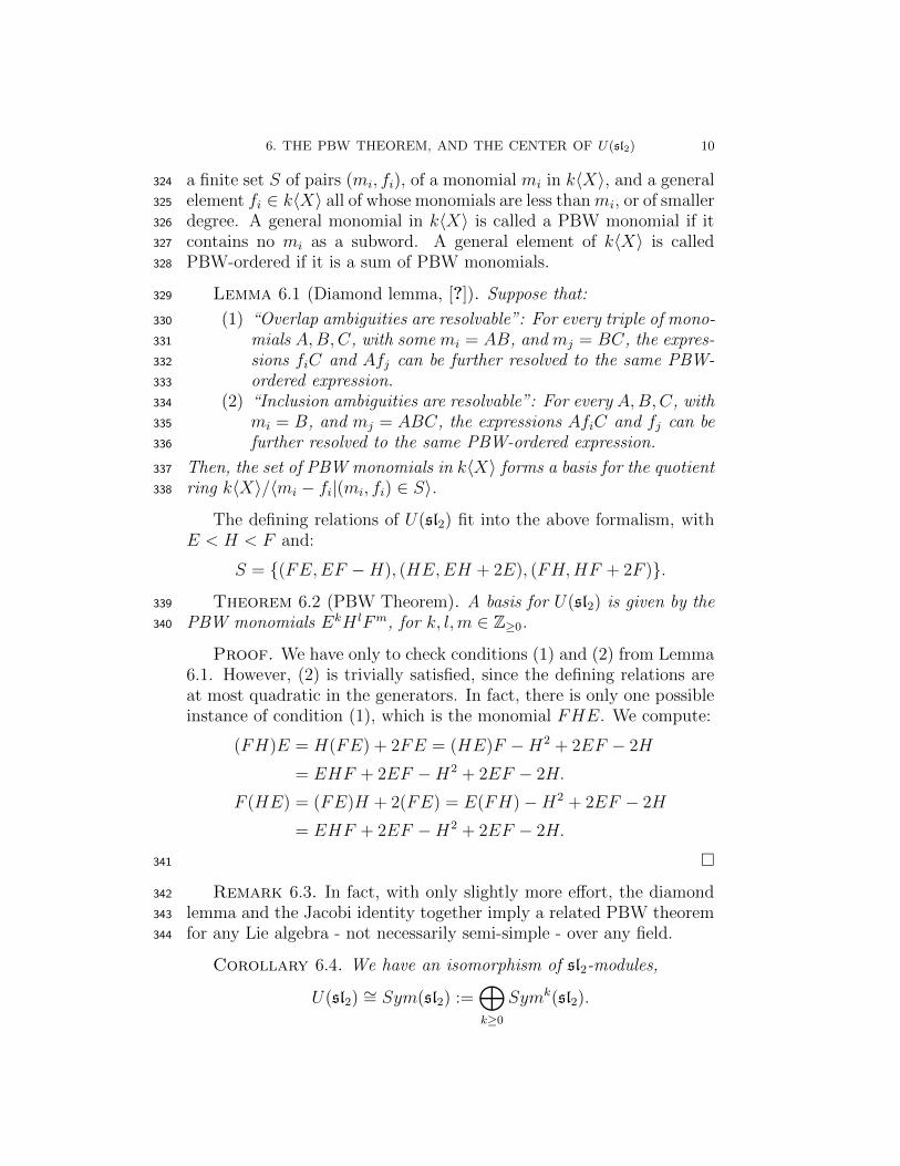
S = {(FE,EF −H), (HE,EH + 2E), (FH,HF + 2F )}.Theorem 6.2 (PBW Theorem). A basis for U(sl2) is given by the339

PBW monomials EkH lFm, for k, l,m ∈ Z≥0.340

Proof. We have only to check conditions (1) and (2) from Lemma6.1. However, (2) is trivially satisfied, since the defining relations areat most quadratic in the generators. In fact, there is only one possibleinstance of condition (1), which is the monomial FHE. We compute:

(FH)E = H(FE) + 2FE = (HE)F −H2 + 2EF − 2H

= EHF + 2EF −H2 + 2EF − 2H.

F (HE) = (FE)H + 2(FE) = E(FH)−H2 + 2EF − 2H

= EHF + 2EF −H2 + 2EF − 2H.

�341

Remark 6.3. In fact, with only slightly more effort, the diamond342

lemma and the Jacobi identity together imply a related PBW theorem343

for any Lie algebra - not necessarily semi-simple - over any field.344

Corollary 6.4. We have an isomorphism of sl2-modules,

U(sl2) ∼= Sym(sl2) :=�

k≥0

Symk(sl2).

6. THE PBW THEOREM, AND THE CENTER OF U(sl2) 11

Proof. Define a filtration, F •, of sl2-modules on U(sl2) by declar-ing each of E,H, F to be of degree one. Then it follows from Theorem6.2 that the associated graded algebra,

grU(sl2) = ⊕k≥0FkU(sl2)/Fk−1U(sl2),

is isomorphic to the symmetric algebra, Sym(sl2). However, since each345

F• is a finite-dimensional sl2-module, and hence semi-simple, we have346

an isomorphism U(sl2) ∼= grU(sl2). �347

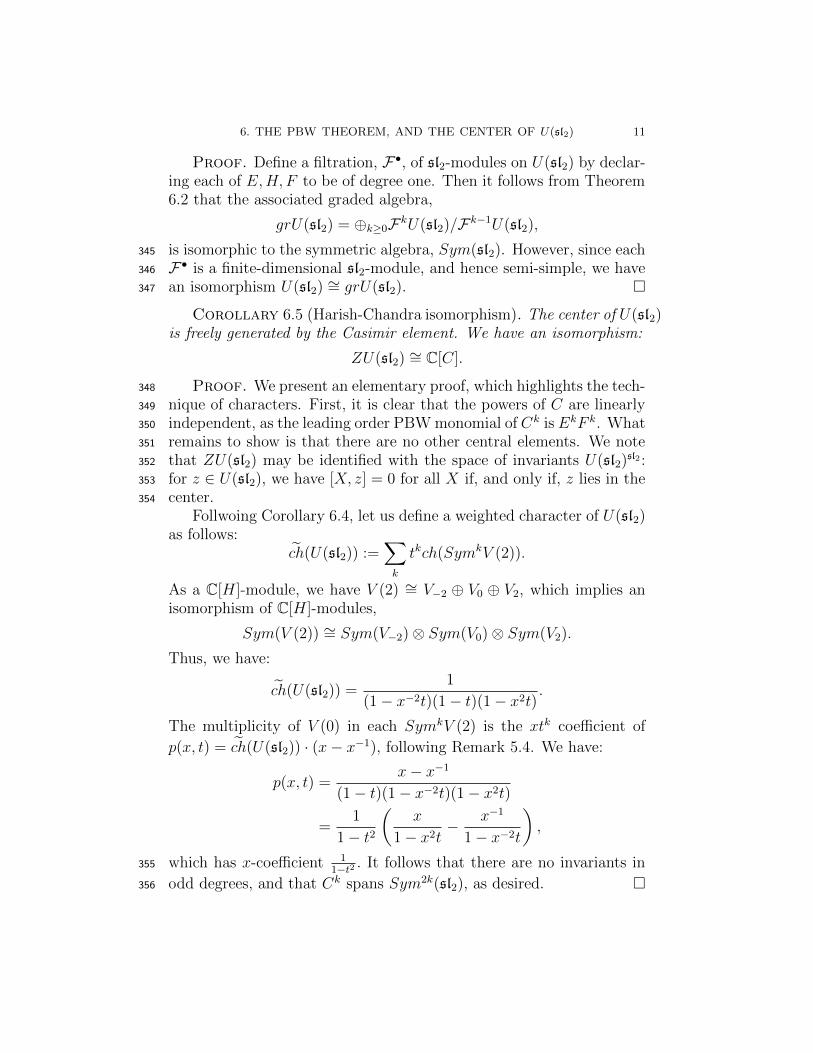
Corollary 6.5 (Harish-Chandra isomorphism). The center of U(sl2)is freely generated by the Casimir element. We have an isomorphism:

ZU(sl2) ∼= C[C].

Proof. We present an elementary proof, which highlights the tech-348

nique of characters. First, it is clear that the powers of C are linearly349

independent, as the leading order PBW monomial of Ck is EkF k. What350

remains to show is that there are no other central elements. We note351

that ZU(sl2) may be identified with the space of invariants U(sl2)sl2 :352

for z ∈ U(sl2), we have [X, z] = 0 for all X if, and only if, z lies in the353

center.354

Follwoing Corollary 6.4, let us define a weighted character of U(sl2)as follows:

�ch(U(sl2)) :=�

k

tkch(SymkV (2)).

As a C[H]-module, we have V (2) ∼= V−2 ⊕ V0 ⊕ V2, which implies anisomorphism of C[H]-modules,

Sym(V (2)) ∼= Sym(V−2)⊗ Sym(V0)⊗ Sym(V2).

Thus, we have:

�ch(U(sl2)) =1

(1− x−2t)(1− t)(1− x2t).

The multiplicity of V (0) in each SymkV (2) is the xtk coefficient of

p(x, t) = �ch(U(sl2)) · (x− x−1), following Remark 5.4. We have:

p(x, t) =x− x−1

(1− t)(1− x−2t)(1− x2t)

=1

1− t2

�x

1− x2t− x−1

1− x−2t

�,

which has x-coefficient 11−t2 . It follows that there are no invariants in355

odd degrees, and that Ck spans Sym2k(sl2), as desired. �356

CHAPTER 2

Hopf algebras and tensor categories357

12

1. HOPF ALGEBRAS 13

1. Hopf algebras358

In Example 1.4 of Chapter 1, for any g-modules V and W , we359

endowed the vector space V ⊗W with a g-module structure. In this360

section, we consider a general class of associative algebras called Hopf361

algebras, which come equipped with a natural tensor product operation362

on their categories of modules. The enveloping algebra U(sl2) will be363

our first example. To begin, let us re-phrase the axioms for an algebra364

in a convenient categorical fashion.365

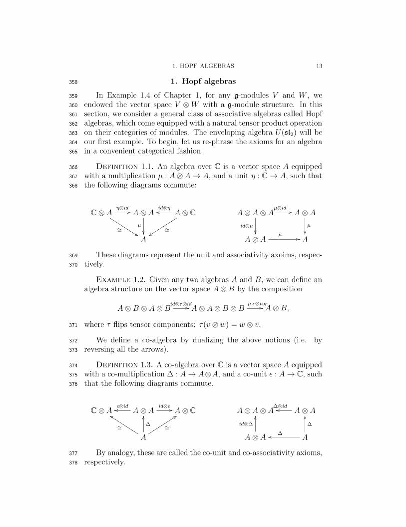
Definition 1.1. An algebra over C is a vector space A equipped366

with a multiplication µ : A⊗A→ A, and a unit η : C→ A, such that367

the following diagrams commute:368

C⊗ A

∼=�������������

η⊗id �� A⊗ A

µ

��

A⊗ Cid⊗η��

∼=�������������

A⊗ A⊗ A

id⊗µ��

µ⊗id �� A⊗ A

µ

��A A⊗ A

µ �� A

These diagrams represent the unit and associativity axoims, respec-369

tively.370

Example 1.2. Given any two algebras A and B, we can define analgebra structure on the vector space A⊗ B by the composition

A⊗ B ⊗ A⊗ Bid⊗τ⊗id�� A⊗ A⊗ B ⊗ B

µA⊗µB�� A⊗ B,

where τ flips tensor components: τ(v ⊗ w) = w ⊗ v.371

We define a co-algebra by dualizing the above notions (i.e. by372

reversing all the arrows).373

Definition 1.3. A co-algebra over C is a vector space A equipped374

with a co-multiplication Δ : A→ A⊗A, and a co-unit � : A→ C, such375

that the following diagrams commute.376

C⊗ A A⊗ A�⊗id�� id⊗� �� A⊗ C A⊗ A⊗ A A⊗ A

Δ⊗id��

A

∼=

�������������∼=

�������������Δ

��

A⊗ A

id⊗Δ

��

A��

Δ

��

By analogy, these are called the co-unit and co-associativity axioms,377

respectively.378

1. HOPF ALGEBRAS 14

Remark 1.4. For any co-algebra A, A∗ becomes an algebra, viathe composition

µ : A∗ ⊗ A∗ �→ (A⊗ A)∗Δ∗−→ A∗

of the natural inclusion , and the dual to the comultiplication map. ifA is a finite-dimensional algebra, then A∗ becomes a co-algebra, viathe composition,

Δ : Aµ∗−→ (A⊗ A)∗ ∼= A∗ ⊗ A∗.

However, for A infinite dimensional, this prescription does not lead to379

a comultiplication map for A∗, since the inclusion A∗⊗A∗ �→ (A⊗A)∗380

is not an isomorphism. In the next chapter we’ll see a way around this381

difficulty.382

Example 1.5. Given two co-algebras A and B, we can define aco-algebra structure on vector space A⊗ B by

A⊗ BΔ⊗Δ �� A⊗ A⊗ B ⊗ B

id⊗τ⊗id�� A⊗ B ⊗ A⊗ B

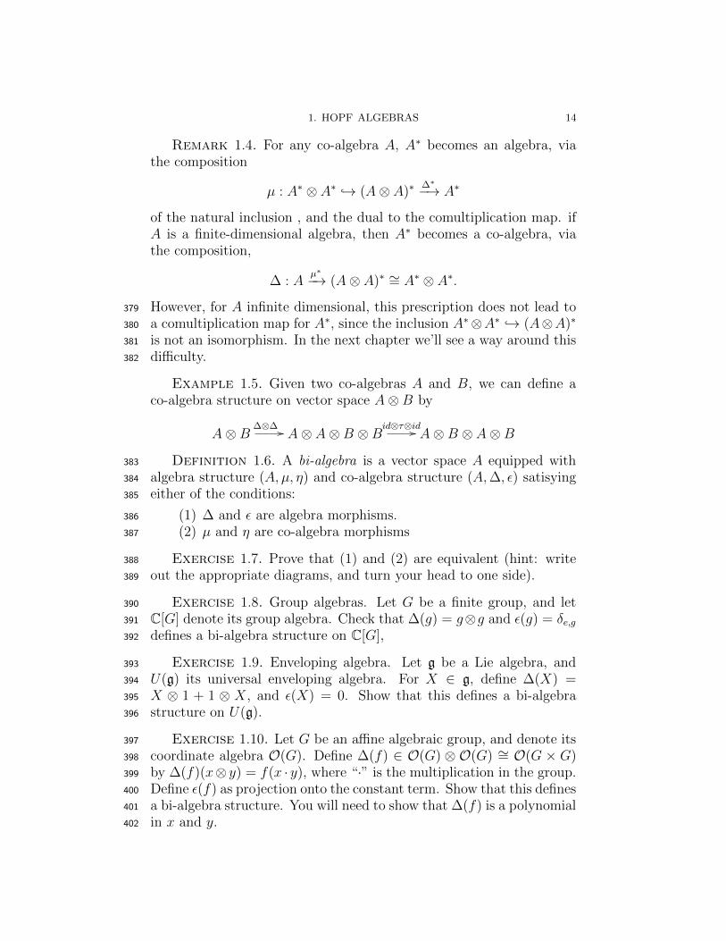
Definition 1.6. A bi-algebra is a vector space A equipped with383

algebra structure (A, µ, η) and co-algebra structure (A,Δ, �) satisying384

either of the conditions:385

(1) Δ and � are algebra morphisms.386

(2) µ and η are co-algebra morphisms387

Exercise 1.7. Prove that (1) and (2) are equivalent (hint: write388

out the appropriate diagrams, and turn your head to one side).389

Exercise 1.8. Group algebras. Let G be a finite group, and let390

C[G] denote its group algebra. Check that Δ(g) = g⊗g and �(g) = δe,g391

defines a bi-algebra structure on C[G],392

Exercise 1.9. Enveloping algebra. Let g be a Lie algebra, and393

U(g) its universal enveloping algebra. For X ∈ g, define Δ(X) =394

X ⊗ 1 + 1 ⊗ X, and �(X) = 0. Show that this defines a bi-algebra395

structure on U(g).396

Exercise 1.10. Let G be an affine algebraic group, and denote its397

coordinate algebra O(G). Define Δ(f) ∈ O(G) ⊗ O(G) ∼= O(G × G)398

by Δ(f)(x⊗ y) = f(x · y), where “·” is the multiplication in the group.399

Define �(f) as projection onto the constant term. Show that this defines400

a bi-algebra structure. You will need to show that Δ(f) is a polynomial401

in x and y.402

1. HOPF ALGEBRAS 15

Exercise 1.11. Let H be a bialgebra, and let I ⊂ H be an ideal403

(with respect to the algebra structure) such that Δ(I) ⊂ H⊗I+I⊗H404

(i.e. I is a co-ideal). Show that Δ and � descend, to form a bi-algebra405

structure on H/I.406

Definition 1.12. Let A be a co-algebra, B an algebra. Let f, g :A→ B be linear maps. We define the convolution product f ∗ g as thecomposition:

AΔ �� A⊗ A

f⊗g �� B ⊗ Bµ �� B

If A is a bialgebra, then taking B = A above yields the structure407

of an associative algebra on End(A), with unit η ◦ �.408

Definition 1.13. A Hopf algebra is a bi-algebra H such that there409

exists an inverse S : H → H to Id relative to ∗: that is, we have410

S ∗ id = id ∗ S = η ◦ �. S is called the antipode.411

Remark 1.14. Note that the antipode on a bi-algebra is unique, if412

it exists, by uniqueness of inverses in the associative algebra End(A).413

The best way to understand the antipode is as a sort of linearized414

inverse, as the following examples illustrate.415

Exercise 1.15. Define S for Examples 1.8, 1.9, 1.10, and show416

that it defines a Hopf algebra in each case.417

Exercise 1.16. (??, III.3.4) In any Hopf algebra, S(xy) = S(y)S(x).418

Hint: Define ν, ρ ∈ Hom(H ⊗ H,H) by ν(x ⊗ y) = S(y)S(x), and419

ρ(x⊗ y) = S(xy). Then compute ρ ∗ µ = µ ∗ ν = η ◦ �.420

Remark 1.17. In the case that S is invertible, it is an anti-automorphism421

and thus can be used to interchange the category of left and right mod-422

ules over H.423

Exercise 1.18. Suppose that the Hopf algebra H is either commu-424

tative, or co-commutative. Show by direct computation that S2 ∗ S =425

η ◦ τ , and thus conclude that S is an involution.426

Definition 1.19. For any bi-algebra H, and H-modules M andN , we define their tensor product M ⊗N to have as underlying vectorspaces the usual tensor product over C, with H-action defined by:

H ⊗ (M ⊗N)Δ⊗id�� H ⊗H ⊗M ⊗N

τ23 �� H ⊗M ⊗H ⊗NµM⊗µN�� M ⊗N

Exercise 1.20. Check that M ⊗ N is in fact an H-module, by427

verifying the associativity and unit axioms.428

2. THE FIRST EXAMPLES OF HOPF ALGEBRAS 16

Exercise 1.21. Similarly, given two H-comodules M and N , we429

can define a comodule structure on their tensor product. Define the430

action, and check that it gives a well-defined co-module structure.431

Remark 1.22. In Examples 1.8, 1.9, 1.10, we recover in this way432

the usual action on M ⊗ N . For instance if G is a group, then in433

k[G], we have g(v ⊗ w) = g(v) ⊗ g(w); if g is a Lie algebra, we have434

x(v ⊗ w) = x(v)⊗ w + v ⊗ x(w).435

2. The first examples of Hopf Algebras436

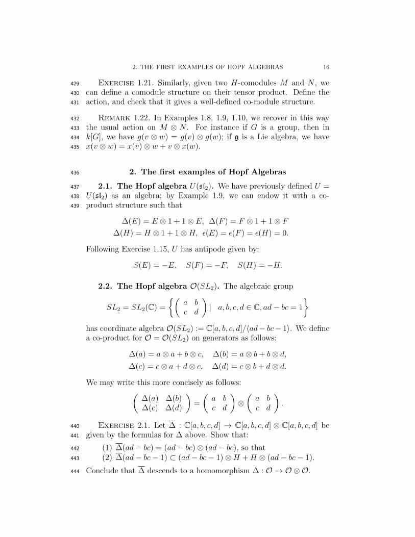
2.1. The Hopf algebra U(sl2). We have previously defined U =437

U(sl2) as an algebra; by Example 1.9, we can endow it with a co-438

product structure such that439

Δ(E) = E ⊗ 1 + 1⊗ E, Δ(F ) = F ⊗ 1 + 1⊗ F

Δ(H) = H ⊗ 1 + 1⊗H, �(E) = �(F ) = �(H) = 0.

Following Exercise 1.15, U has antipode given by:

S(E) = −E, S(F ) = −F, S(H) = −H.

2.2. The Hopf algebra O(SL2). The algebraic group

SL2 = SL2(C) =

��a bc d

�| a, b, c, d ∈ C, ad− bc = 1

�

has coordinate algebra O(SL2) := C[a, b, c, d]/�ad− bc− 1�. We definea co-product for O = O(SL2) on generators as follows:

Δ(a) = a⊗ a + b⊗ c, Δ(b) = a⊗ b + b⊗ d,

Δ(c) = c⊗ a + d⊗ c, Δ(d) = c⊗ b + d⊗ d.

We may write this more concisely as follows:�

Δ(a) Δ(b)Δ(c) Δ(d)

�=

�a bc d

�⊗�

a bc d

�.

Exercise 2.1. Let Δ : C[a, b, c, d] → C[a, b, c, d] ⊗ C[a, b, c, d] be440

given by the formulas for Δ above. Show that:441

(1) Δ(ad− bc) = (ad− bc)⊗ (ad− bc), so that442

(2) Δ(ad− bc− 1) ⊂ (ad− bc− 1)⊗H + H ⊗ (ad− bc− 1).443

Conclude that Δ descends to a homomorphism Δ : O → O ⊗O.444

3. TENSOR CATEGORIES 17

This makes O(SL2) into a bi-algebra. We now introduce an an-tipode, which will endow it with the structure of a Hopf algebra. Wedefine S on generators:�

S(a) S(b)S(c) S(d)

�=

�d −b−c a

�.

Exercise 2.2. Verify that S is an antipode.445

3. Tensor Categories446

In the previous section, we saw that for any Hopf algebra H, the447

category of H-modules has a tensor product structure. In this section,448

we will define the notion of a tensor category, which captures this prod-449

uct structure. The reason for the focus on categorical constructions is450

that when we look at the quantum analogs of our classical objects,451

much of the geometric intuition fades, while the categorical notions452

remain largely intact.453

Definition 3.1. Let C,D be categories. Their product, C × D, isthe category whose objects are pairs (V,W ), V ∈ ob(C),W ∈ ob(D),and whose morphisms are given by:

Mor((U, V ), (U �, V �)) = Mor(U,U �)×Mor(V, V �).

Let ⊗ be a functor ⊗ : C × C → C. This means that for each pair454

(U, V ) ∈ C ×C, we have their tensor product U ⊗ V , and for any maps455

f : U → U �, g : V → V �, we have a map f ⊗ g : U ⊗ V → U � ⊗ V �.456

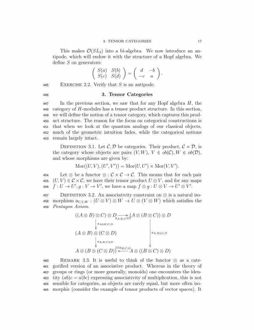
Definition 3.2. An associativity constraint on ⊗ is a natural iso-457

morphism aU,V,W : (U ⊗ V ) ⊗W → U ⊗ (V ⊗W ) which satisfies the458

Pentagon Axiom.459

((A⊗ B)⊗ C)⊗D

aA⊗B,C,D

��

aA,B,C⊗1�� (A⊗ (B ⊗ C))⊗D

aA,B⊗C,D

��

(A⊗ B)⊗ (C ⊗D)

aA,B,C⊗D

��A⊗ (B ⊗ (C ⊗D)) A⊗ ((B ⊗ C)⊗D)

1⊗aB,C,D��

Remark 3.3. It is useful to think of the functor ⊗ as a cate-460

gorified version of an associative product. Whereas in the theory of461

groups or rings (or more generally, monoids) one encounters the iden-462

tity (ab)c = a(bc) expressing associativity of multiplication, this is not463

sensible for categories, as objects are rarely equal, but more often iso-464

morphic (consider the example of tensor products of vector spaces). It465

3. TENSOR CATEGORIES 18

is an exercise to show that the basic associative identity for monoids466

implies that any two parenthesizations of the same word of arbitrary467

length are equal. In tensor categories, we need to impose an equal-468

ity of various associators on tensor products of quadruples of objects.469

MacLane’s theorem [] asserts that this commutativity on 4-tuples im-470

plies the analogous equality of associators for n-tuples, so that we may471

omit parenthesizations going forward.472

Definition 3.4. A unit for ⊗ is a triple (I, l, r), where I ∈ C, and473

l : I ⊗ U → U and r : U ⊗ I → I are natural isomorphisms.474

Definition 3.5. A tensor category is a collection (C,⊗, a, I, l, r)with a, I, l, r as above, such that we have the following commutativediagram

(A⊗ I)⊗ Ba ��

���������A⊗ (I ⊗ B)

���������

A⊗ B

.

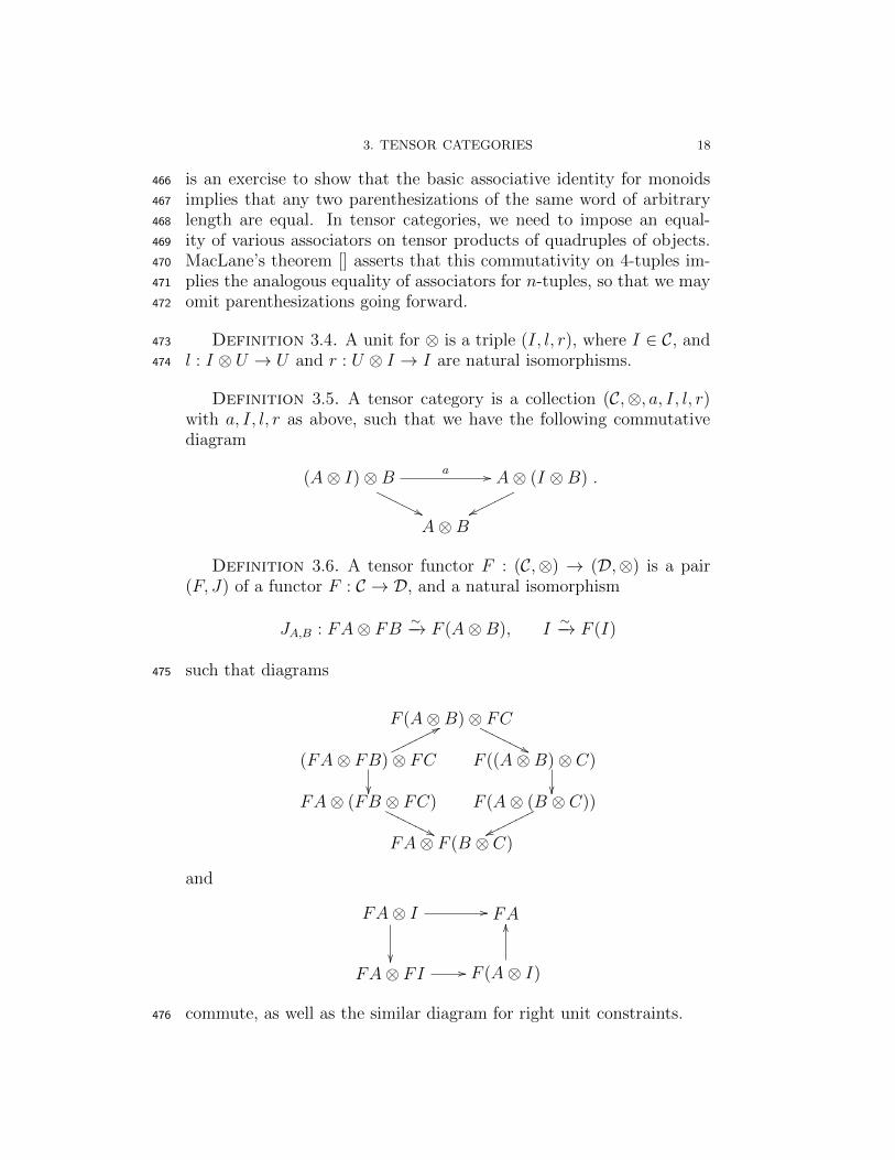
Definition 3.6. A tensor functor F : (C,⊗) → (D,⊗) is a pair(F, J) of a functor F : C → D, and a natural isomorphism

JA,B : FA⊗ FB∼−→ F (A⊗ B), I

∼−→ F (I)

such that diagrams475

FA⊗ (FB ⊗ FC)

FA⊗ F (B ⊗ C)

F (A⊗ (B ⊗ C))

(FA⊗ FB)⊗ FC

F (A⊗ B)⊗ FC

F ((A⊗ B)⊗ C)

������������

���������� ����������

��

����������

and

FA⊗ I ��

��

FA

FA⊗ FI �� F (A⊗ I)

��

commute, as well as the similar diagram for right unit constraints.476

3. TENSOR CATEGORIES 19

Definition 3.7. A tensor natural transformation between tensorfunctors F and G is a natural transformation α : F → G is such that

FA⊗ FB

��

�� F (A⊗ B)

��GA⊗GB �� G(A⊗ B)

commutes.477

478

Definition 3.8. (C,⊗) is strict if a, l, r are all equalities in the479

category (meaning that the underlying objects are equal, and the mor-480

phism is the identity). A tensor functor F = (F, J) is strict if J is an481

equality and I = FI.482

Remark 3.9. Most categories arising naturally in representation483

theory are not strict categories, but we will see in chapter ?? by an484

extension of MacLane’s coherence theorem that any tensor category is485

tensor equivalent to a strict category. In chapter ??, we will see some486

examples of strict tensor categories.487

Example 3.10.488

CHAPTER 3

Geometric Representation Theory for SL2489

20

1. THE ALGEBRA OF MATRIX COEFFICIENTS 21

In this chapter we begin the study of geometric representation the-490

ory, in which techniques from algebraic and differential geometry are491

brought to bear on the representation theory of algebraic groups. We492

focus on three main results:493

(1) the Peter-Weyl Theorem, which states that the coordinate al-494

gebra O(G), viewed as a left G × G-module, contains one di-495

rect summand End(V ) for every finite dimensional irreducible496

module V of G;497

(2) the Borel-Weil theorem, which realizes finite-dimensional rep-498

resentations of a semi-simple algebraic group geometrically as499

sections of certain equivariant line bundles on the correspond-500

ing flag variety; and501

(3) the Beilinson-Bernstein localization theorem, which gives an502

equivalence between the category of D-modules on the flag503

variety and the category of U(g)-modules with trivial central504

character.505

As in the previous chapter, we will look to SL2 for most of our exam-506

ples.507

1. The algebra of matrix coefficients508

The finite dimensional representations of a (possibly infinite dimen-sional) Hopf algebra H determine a natural subalgebra of H∗, calledthe algebra of matrix coefficients, which is naturally a Hopf algebra,thus overcoming the finiteness issues in Remark ??. The dual vectorspace H∗ carries an action of H ⊗H, given by:

((a⊗ b)φ)(x) := φ(S(b)xa).

Definition 1.1. The external tensor product V �W of H-modules509

V and W is the H ⊗H-module with underlying vector space V ⊗C W ,510

and action (u1 ⊗ u2)(v ⊗ w) := u1v ⊗ u2w.511

Let V be a finite dimensional H-module. For f ∈ V ∗, v ∈ V ,512

the matrix coefficients cVf,v ∈ H∗ are defubed by cVf,v(u) := f(u.v), for513

u ∈ H. The assignment (f, v) �→ cVf,v is bi-linear; we thus obtain a514

linear map cV : V ∗ � V → H∗.515

Exercise 1.2. Show that cVf,vcWg,w = cV⊗W

g⊗f,v⊗w.516

Exercise 1.3. Let φ : V → W be a homomorphism of H-modules.517

Show that, for v ∈ V, f ∈ W ∗, we have cWf,φv = cVφ∗f,v.518

Definition 1.4. The algebra, O, of matrix coefficients, is the linear519

subspace of H∗ spanned by the cf,v for all finite-dimensional. V .520

2. PETER-WEYL THEOREM FOR SL(2) 22

Exercise 1.5. Conclude that O is a H⊗H-submodule of H∗, andthat cV is a H ⊗H-module map, by showing, for a, b ∈ H:

(a⊗ b)cf,v = cbf,av.

Exercise 1.6. Fix a basis v1, . . . , vn for V , and let f1, . . . , fn for V ∗521

be the dual basis. Verify that the representation map ρ : U → gl(V )522

sends x to the matrix (cfi,vi(x))ni,j=1, thus justifying the name “matrix523

coefficient”.524

Exercise 1.7. Suppose that H is commutative, or co-commutative,525

so that the tensor flip v ⊗ w �→ w ⊗ v is a morphism of H-modules.526

Show in this case that O is commutative.527

Proposition 1.8. Let Δ : H∗ → (H ⊗H)∗ denote the dual to the528

multiplication map on H. Then we have Δ(O) ⊂ O ⊗O ⊂ (H ⊗H)∗,529

and this endows O with the structure of a Hopf algebra.530

Proof. For the first claim, it suffices to show that Δcf,v ∈ O⊗O,531

for each finite-dimensional V , each f ∈ V ∗, and v ∈ V . Let {vi} be a532

basis for V and {fi} a dual basis for V ∗. The proof follows from the533

following exercise:534

Exercise 1.9. Show that Δ(cf,v) =�n

i=1 cf,vi ⊗ cfi,v, by checking535

that this expression satisfies: �Δ(cf,v), x⊗ y� = �cf,v, xy�.536

Having defined the bi-algebra structure, the antipode S is defined537

by �S(cf,v), x� = �cf,v, S(x)�, for x ∈ H.538

�539

2. Peter-Weyl Theorem for SL(2)540

Returning to the case U = U(sl2), we have the following description541

of the algebra O of matrix coefficients.542

Theorem 2.1. (Peter-Weyl) Let V (n) denote the irreducible rep-resentation of sl2 of highest weight n. Then we have an isomorphismof U ⊗ U-modules:

O ∼=∞�

j=0

V (j)∗ � V (j),

Proof. We have a map of U ⊗ U -modules,∞�

j=0

cV (j) :∞�

j=0

V (j)∗ � V (j)→ O.

Each cV (j) is an injection: the kernel is a submodule of the irreducible543

U ⊗ U -module V (j)∗ ⊗ V (j), and each cV (j) is clearly not identically544

3. RECONSTRUCTING O(SL2) FROM U(sl2) VIA MATRIX COEFFICIENTS.23

zero. Moreover, the images of cV (j) and cV (k) must intersect trivially,545

for j �= k, since these are non-isomorphic irreducible submodules.546

It only remains to prove surjectivity; we need to show that O is infact contained in the sum of of the images of the maps cV (i). For this,let V be an arbitrary finite dimensional representation, and using thesemi-simplicity proved in Chapter 1, write V as a finite direct sum ofirreducibles:

V ∼=N�

i=0

V (i)⊕mi .

Let πi,j and ιi,j , respectively, denote the projection onto, and inclusioninto, the jth copy of V (i) in the sum. We clearly have π∗

i,j = ιi,j . Letf ∈ V ∗, v ∈ V . Then we may write:

v =�

i,j

ιi,jvi,j , f =�

k,l

π∗k,lfk,l,

for some collection of vi,j ∈ V (i) and fk,l ∈ V (i)∗. Thus, we have:

cVf,v =�

i,j,k,l

cVπ∗k,lfk,l,ιi,jvi,j

=�

i,j,k,l

cVfk,l,πk,lιi,jvi,j .

We have πk,lιi,j = IdV (i) if i = k, and 0 otherwise. Thus the right hand547

side lies in the span of the images of the maps cV (i), as desired. �548

Remark 2.2. Clearly, both the statement and proof of the Peter-549

Weyl theorem apply mutatis mutandis for any semi-simple algebraic550

groups.551

3. Reconstructing O(SL2) from U(sl2) via matrix coefficients.552

Choose a basis v1, v2 of V (1), and let v1, v2 denote the dual basis ofV (1)∗. We use the notation cij := cvi⊗vj . We denote by i0 and π0 themaps:

i0 : V (0)→ V (1)⊗ V (1), π0 : V (1)∗ ⊗ V (1)∗ → V (0)

1 �→ v1 ⊗ v2 − v2 ⊗ v1�

aijvi ⊗ vj �→ (a12 − a21)

Thus i0 and π0 are the inclusion and projection, respectively, of thetrivial representation relative to the decomposition,

V (1)⊗ V (1) ∼= V (2)⊕ V (0).

Exercise 3.1. The purpose of this exercise is to construct an iso-553

morphism between O(SL2) and the algebra O of matrix coefficients on554

U(sl2).555

4. EQUIVARIANT VECTOR BUNDLES, AND SHEAVES 24

(1) Show that there exists a unique homomorphism:

φ : C[a, b, c, d]→ O,

(a, b, c, d) �→ (c11, c12, c

21, c

22).

(2) Show that φ is surjective, using the fact that V (1) generates556

the tensor category of sl2 modules.557

(3) Show that the relations cf,i0(v) = cπ0(f),v, for f = v1, v2 and558

v = v1, v2, reduce to the single relation ad− bc = 1.559

(4) The algebra O(SL2) = C[a, b, c, d]/�ad − bc − 1� admits a fil-tration with generators a, b, c, d in degree one. Let Fi denotethe ith filtration, and show that Fi/Fi−1 has a basis:

Bi = {akdlcm | k + l + m = i} ∪ {akdlbm | k + l + m = i},so that dimFi/Fi+1 = |Bi| = 2

�i+22

�− (i + 1) = (i + 1)2.560

(5) Show that φ is a map of filtered vector spaces, where

Fi(O) = ⊕k≤iV (k)∗ � V (k).

(6) Conclude that φ is injective, and thus an isomorphism of al-561

gebras.562

Exercise 3.2. Show that φ is a isomorphism of Hopf algebras, by563

showing that it respects co-products.564

Remark 3.3. This exercise is the easiest case of a very general the-565

ory, called Tannaka-Krein Reconstruction, which gives a prescription566

for recovering the coordinate algebra of a reductive algebraic group567

(more generally, any Hopf algebra) from its category of finite dimen-568

sional representations.569

4. Equivariant vector bundles, and sheaves570

Let X be an algebraic variety over C, and G an algebraic group.Let us denote the multiplication map on G by mult:

G×Gmult−→ G

Suppose G acts on X, meaning that we have an algebraic morphism:

G×Xact−→ X

which is associative:

act ◦ (mult× 1) = (act) ◦ (1× act) : G×G×X → X

Definition 4.1. A G-equivariant vector bundle on X is a vector571

bundle π : V → X, over X, together with an action G × V → V572

commuting with π, and restricting to a linear map φg,x : Vx → Vgx of573

each fiber.574

4. EQUIVARIANT VECTOR BUNDLES, AND SHEAVES 25

It follows that the maps φg,x are linear isomorphisms, and are as-sociative in the following sense:

φh,gx ◦ φg,x = φhg,x.

We will now give a generalization of this definition to sheaves. Us-ing the multiplication, action and projection we can form three maps,d0, d1, d2 : G×G×X → G×X:

d0(g1, g2, x) = (g2, g−11 x), d1(g1, g2, x) = (g1g2, x),

d2(g1, g2, x) = (g1, x).

We also have the identity section from s : X → G × X, s(x) = (e, x),575

and the projection proj : G×X → X, proj(g, x) = x.576

Definition 4.2. A G-equivariant sheaf on X is a pair (F , θ), whereF is a sheaf on X and θ is an isomorphism,

θ : proj∗F −→ act∗Fsatisfying the cocycle and unit conditions:

d∗0θ ◦ d∗2θ = d∗1θ, s∗θ = idF .

Exercise 4.3. Prove that if V is an equivariant vector bundle then577

the locally free sheaf of sections of V is an equivariant sheaf.578

Exercise 4.4. Prove that if V is a G-equivariant locally free sheaf579

on X, then SpecX(V ), the associated vector bundle on X is a G-580

equivariant vector bundle.581

Remark 4.5. Note that the we can give this definition also in other582

categories (topological, differentiable, analytic,...).583

Suppose now that X = Spec(A) is an affine variety and G =584

Spec(H) is an affine algebraic group, so that H is a commutative Hopf585

algebra. The action of G on X translates into A being a H-comodule586

algebra:587

Definition 4.6. An H-comodule algebra A is an H-comodule, and588

an algebra, such that the multiplication map m : A⊗A→ A is a map589

of comodules, where A⊗ A is an H-module via tensor product.590

Definition 4.7. The category CHA of H-equivariant A-modules has591

as objects H-comodules M , equipped with a map m : A ⊗M → M592

of H-comodules, making M into an A-module. The morphisms in this593

category are the maps that commute with both the A-module structure594

and the H-comodule structure.595

5. QUASI-COHERENT SHEAVES ON THE FLAG VARIETY 26

Exercise 4.8. In the setup of the preceding paragraph, construct596

an equivalence between CHA and the category of G-equivariant sheaves597

on X.598

Exercise 4.9. Suppose that G acts transitively on X. Show that599

a G-equivariant sheaf is locally free (hint: produce an isomorphism on600

stalks, Fx → Fgx).601

Exercise 4.10. Let X = G, and let G act on itself by left multipli-602

cation. Show that the category of quasi-coherent G-equivariant sheaves603

of OG-modules is equivalent to the category of vector spaces.604

Exercise 4.11. Let X = {pt} with the trivial G-action. Show605

that the category of G-equivariant sheaves on X is equivalent to the606

category of representations of G.607

5. Quasi-coherent sheaves on the flag variety608

For any semi-simple algebraic group, the flag variety is a homoge-neous space, the quotient G/B of G by its Borel subgroup B. In thecase G = SL2, the Borel subgroup B is the set of upper-triangularmatrices,

B =

�a b0 a−1

�.

We may identify B with the stabilizer of the line spanned by the first609

basis vector; the orbit-stabilizer theorem then gives an identification of610

G/B with the first projective space P1.611

While G/B is a projective variety – in particular, not affine – we can612

nevertheless approach its category of quasi-coherent sheaves without613

appeal to projective geometry, by describing quasi-coherent sheaves on614

G/B as B-equivariant sheaves on G. This purely algebraic point of615

view will most easily generalize to the quantum case considered in the616

next chapter, where most of the geometry is necessarily expressed in617

algebraic terms.618

Definition 5.1. The category of quasi-coherent sheaves on the619

coset space G/B, denotedQCoh(G/B), has as objects all B-equivariant620

O-modules on G. Morphisms in QCoh(G/B) are those which commute621

with both the O action and the O(B)-coaction.622

Remark 5.2. It is a theorem due to [] that the flag variety is in623

fact an algebraic variety, and that furthermore its category of quasi-624

coherent sheaves is equivalent to the category we have defined above.625

Remark 5.3. Because the G-action is transitive, we can identify626

the fibers of the sheaf for all x ∈ G/B.627

5. QUASI-COHERENT SHEAVES ON THE FLAG VARIETY 27

More generally, for any Hopf we have a Hopf algebra H. The next628

lemma generalizes Exercise 4.10.629

Proposition 5.4. CHH ∼ Vect.630

Proof. Let M co−inv = {m ∈M |Δm = m⊗1}, then M �→M co−inv631

defines a functor F : CH → Vect. The assignment V �→ V ⊗ H gives632

a functor G : Vect → CH . To finish the proof, we need to produce633

natural isomorphisms M ∼= H ⊗M co−inv and (V ⊗H)co−inv ∼= V . �634

Suppose H has a quotient Hopf algebra A. We define a category635

ACH as the category whose objects are H-modules M with a right O-636

comodule and left A-module structures, such that H ⊗M → M is an637

A-comodule map and H-comodule map.638

Here we use HΔ−→ H ⊗ H → A ⊗ H to give H an A-comodule639

structure.640

Lemma 5.5. ACH ∼ Left A-modules.641

Proof. This is an easy extension of Proposition 5.4. �642

Since G = SL(2) is an affine algebraic variety, the quasi-coherent643

sheaves on G are just the O(SL(2)) modules. In this case, the Borel644

subgroup is the group U of upper triangular matrices. Thus, we can645

construct the category of P1-modules as the category of O(SL(2)) mod-646

ules M which have O(U)-comodule action, such that O(SL(2)⊗M →647

M is both an O(SL(2))-module map, and a O(U)-comodule map. This648

gives us our first description of quasi-coherent modules on P1.649

There is a second, less general, construction of quasi-coherent sheaves650

on P1, which will give us a more explicit description. We note that U =651

T � N , where T ∼= C× is the group of diagonal matrices, and N ∼= C652

is the group of unipotent matrices. Thus, SL(2)/U ∼= (SL(2)/N)/T .653

N =

��1 b0 1

��, U =

��a b0 a−1

��, T =

��a 00 a−1

��, a, b ∈ C.

Exercise 5.6. SL(2)/N ∼= A2◦, where A2 = Spec(C[x, y]), and A2

◦654

denotes A2\{0}. It may be helpful to think of A2◦ as the space of based655

lines {(l, v)|0 �= v ∈ l ⊂ C2}.656

Now let us describeQCoh(A2◦). We first recall that since A2 is affine,657

QCoh(A2) = C[x, y]-modules.658

Definition 5.7. A C[x, y] module M is torsion if for any m ∈M ,659

there exists an l >> 0 s.t. xlm = ylm = 0.660

6. THE BOREL-WEIL THEOREM 28

We consider the restriction functor Res : QCoh(A2) → QCoh(A2◦).661

This is clearly surjective, since we can always extend a sheaf by zero662

off of an open set.663

Lemma 5.8. Res(M) ∼= 0 if, and only if, M is a torsion sheaf.664

Proof. Let M be a torsion sheaf on A2. On A2\{y-axis}, x is665

invertible, so M is necessarily zero there. Likewise, on A2\{x-axis}, y666

is invertible, so M is zero there. Since these two open sets cover A2◦,667

we can conclude that torsion sheaves are sent to zero under restriction.668

Conversely, if Mx and My are both zero, then M is a torsion sheaf. �669

We would like now to conclude that QCoh(A2◦) is the quotient of670

QCoh(A2) by the full subcategory consisting of torsion modules. In671

order to say this, we must define what we mean by the quotient of672

a category by a subcategory. This is naturally defined whenever the673

categories are abelian, and the subcategory is full, and also closed with674

respect to short exact sequences. These notions, and the quotient con-675

struction, are explained in the appendix ?? on abelian categories.676

Theorem 5.9. QCoh(A2◦) � C[x, y]−modules/torsion.677

Theorem 5.10. QCoh(P1) = graded C[x, y]−modules/torsion.678

Proof. The C∗ action on C[x, y] is dilation of each homogeneous679

component, λ(p(x, y)) = λdeg(p)p(x, y). Thus, an equivariant module680

with respect to this action inherits a grading Mk = {m ∈ M |λ(m) =681

λkm}. Conversely, given a grading we can define the C∗ action accord-682

ingly. �683

Example 5.11. C[x, y], which corresponds to OCP 1 ;684

Example 5.12. If M = ⊕nMn is an object, then M(m) is defined685

by the shifted grading, M(m)n = Mn−m686

Example 5.13. The Serre twisting sheaves are a particular case of687

the last two examples. We have OCP 1(i) = C[x, y](i),688

Definition 5.14. We define the global sections functor for a graded689

C[x, y]-module to just be the zeroeth graded component. Γ(⊕nMn) =690

M0. Clearly, this coincides with the usual definition of global sections691

of an OP1-module.692

6. The Borel-Weil Theorem693

For an algebraic group G, we say that V is an algebraic module ifwe have a map to GL(V ) that is a morphism of group varieties. Givenan algebraic B-module V , we can obtain another algebraic B-module

6. THE BOREL-WEIL THEOREM 29

O(SL(2))⊗V by taking the right action of B on O(SL(2)). This spacealso has a leftO(SL(2))-module structure. So, we can define an inducedO(SL(2))-module

IndSL(2)B (V ) = (O(SL(2))⊗C V )B

where the superscript B denotes that we take the B invariant part694

(only the vectors fixed by B via the action on V and the right action695

on O(SL(2))).696

We analyze how this induction works in more detail. Since weare considering SL(2), we will only need to work with one-dimensionalalgebraic B-modules, which we now characterize. A one-dimensionalrepresentation of C∗ ∼= Gm is a morphism C∗ → C∗ respecting multi-plication, and it’s easy to see that these are the maps z �→ zn. Thereare no non-trivial algebraic representations of C ∼= Ga. Thus, the one-dimensional representations of B are indexed by the integers. We letCn denote the representation

�a b0 a−1

�1n = a−n 1n

We have the following important result.697

Theorem 6.1. (Borel-Weil)698

IndSL(2)B Cn = V (n)∗

Proof. Consider the invariants (O(SL(2))⊗ Cn)B. Note that the

B-invariant submodules correspond exactly to irreducible submodulesV (0), and hence to highest weight vectors of weight 0. We can use thePeter-Weyl theorem to write

(O(SL(2))⊗ Cn)B =

� ∞�

j=0

V (j)∗ ⊗ V (j)⊗ Cn

�B

Note B only acts on the rightmost two factors, so we can reduce to

∞�

j=0

V (j)∗ ⊗ (V (j)⊗ Cn)B

Now, for example, if {v0, . . . , vj} forms a basis for Vj, then {v0 ⊗699

1n, . . . , vj⊗ 1n} is a basis for V (j)⊗Cn. The only vector killed by E is700

vo⊗ 1n, and it has weight j− n. Thus, the only highest weight vectors701

of weight 0 occur when j = n. So, we find IndSL(2)B Cn = V (n)∗. �702

7. BEILINSON-BERNSTEIN LOCALIZATION 30

Remark 6.2. More generally the Borel-Weil theorem implies that703

for G semi-simple, B its Borel sub-algebra, every finite dimensional704

representation of G can be realized by induction from B in this way.705

What is the geometric interpretation of this theorem? We can re-706

late the induced representation to line bundle structures on the quo-707

tient SL(2)/B. By proposition ??, a one dimensional B-module M708

determines a G-equivariant O(G/B) line bundle M . The global sec-709

tions Γ(M) of this line bundle have a G-action, and this module is710

IndGBM . Let’s take a look at our example. We can describe quasi-711

coherent O- modules on P1 ∼= SL(2)/B by considering B-equivariant712

O(SL(2))-modules. Starting from a B-module V , we can obtain such713

equivariant modules by tensoring O(SL(2))⊗C V and taking the right714

B-action on O(SL(2)) as above. For example, starting with Cn, our715

equivariant module will be O(SL(2)) ⊗ Cn. By Borel-Weil the global716

sections of the quotient bundle will be V (n)∗, so we can identify this717

line bundle with the twisting sheaf OP1(n).718

7. Beilinson-Bernstein Localization719

7.1. D-modules on P1. In this section, we will construct certain720

D-modules, which are essentially sets of solutions of algebraic differen-721

tial equations. In section ??, we will define D-modules for any affine722

algebraic variety, but for now, we consider the cases of A2, A2◦ = A2\{0}723

and P1. To consider D-modules on a general algebraic variety, one sim-724

ply sheafifies the construction for affine algebraic varieties.725

Definition 7.1. We define the second Weyl algebra, W, to be the726

algebra generated over C by {x, y, ∂x, ∂y}, subject to relations [x, ∂x] =727

[y, ∂y] = 1, with all other pairs of generators commuting. W is a graded728

algebra over C with deg x = deg y = 1, deg ∂x = deg ∂y = −1.729

Definition 7.2. A D-module on A2 is a module over W730

Definition 7.3. A W -module M is torsion if for all m ∈M , there731

is a k such that xkm = ykm = 0732

A similar consideration to that which led to quasi-coherent sheaves733

on A2◦ yields the following734

Definition 7.4. The category of D-modules on A2◦ is the quotient735

of the category of W -modules by the full subcategory of torsion mod-736

ules.737

W contains a distinguished element, called the Euler operator T =738

x∂x + y∂y. Geometrically, T corresponds to the vector field on A2739

7. BEILINSON-BERNSTEIN LOCALIZATION 31

pointing in the radial direction at every point, and vanishing only at740

the origin. We now use W to define D-modules on P1:741

Definition 7.5. The category of D-modules on P1 has as its ob-742

jects graded W2-modules M modulo torsion such that T acts on the743

nth graded component Mn as scalar multiplication by n.744

Remark 7.6. This graded action by the Euler operator is the cor-745

rect notion of equivariance in the differential setting.746

Example 7.7. The polynomial ring C[x, y] with the usual grading747

is a D-module on P1, where x and y act by left multiplication, and748

∂x and ∂y act by differntiation. More generally, the structure sheaf is749

always a D-module.750

Example 7.8. The shifted modules C[x, y](n) are not D-modules,751

because although they are modules over W , the Euler operator does752

not act on the graded components by the correct scalar.753

Example 7.9. C[x, x−1, y] with grading deg x = deg y = 1 and754

deg x−1 = −1 is a D-module. Note that the global sections functor755

yields Γ(C[x, x−1, y]) = C[x−1y], whereas above we had Γ(C[x, y]) = C.756

7.2. The Localization Theorem. We wish to investigate the757

structure of W a little further. If we decompose it into graded compo-758

nents as W =�

i∈Z Wi, then what is the 0th component W0? Since759

W acts faithfully on C[x, y], it suffices to consider the embedding760

W �→ End(C[x, y]) and answer the same question for the image of761

W .762

Exercise 7.10. The component W0 is generated by the elements763

x∂y, y∂x, x∂x, and y∂y.764

Lemma 7.11. The elements xiyj∂kx∂ly form a basis for W2.765

Proof. Using the commutation relations, it is easy to show that766

these elements are stable under left multiplication by the generators767

of W . Furthermore, since 1 is of this form, these elements must span768

W . Thus it remains only to check the linear independence of these769

elements. This is clear from the faithful action on C[x, y], so we are770

done. �771

Modifying the generating set for W0 slightly to be x∂y, y∂x, T, x∂x−772

y∂y, we now notice a few interesting relations:773

x∂y(x) = 0, y∂x(x) = y, (x∂x − y∂y)(x) = x

x∂y(y) = x, y∂x(y) = 0, (x∂x − y∂y)(y) = −y.

7. BEILINSON-BERNSTEIN LOCALIZATION 32

This is exactly the action of sl(2,C), where we identify the generators774

E = x∂y, F = y∂x, and H = x∂y − y∂x, together with the element T .775

Definition 7.12. Let U be a Hopf algebra acting on a module776

A. Then A is called a module algebra if we have a multiplication µ :777

A⊗A→ A, which is a map of U -modules. Specifically, if Δu = u1⊗u2,778

then we require u(ab) = (u1a)(u2b).779

For the universal enveloping algebra U = U(sl(2,C)) and x ∈780

sl(2,C), we have the comultiplication map Δx = x⊗1+1⊗x, so the def-781

inition of a module algebra imposes the condition x(ab) = (xa)b+a(xb).782

This is precisely the Leibniz rule, so x acts as a derivation. In particu-783

lar, if U(sl(2,C)) acts on C[x, y] as a module algebra, then the genera-784

tors E,F,H act as derivations and so their action coincides with that785

of x∂y, y∂x, x∂x − y∂y. (We leave it as an exercise to check that U acts786

in the correct way.)787

In particular, the action of C�x∂y, y∂x, x∂x−y∂y� ⊂ W ⊂ End(C[x, y])788

is identical to that of U(sl(2,C)). Furthermore, T = x∂x+y∂y is central789

inside W0 since it acts as a scalar on each graded component and thus790

commutes with these degree-preserving generators there. But we know791

that the center of U(sl(2,C)) is generated by the Casimir element C,792

so we can express T as a polynomial in C. Since C acts on C[x, y]i as793

scalar multiplication by i(i + 2), and T acts on it as multiplication by794

i, we must have C = T 2 + 2T . Therefore we have795

W0 = U(sl(2,C))[T ]/�C = T 2 + 2T �.For any D-module M on P1, we get an action of W0 on the global796

sections Γ(M) = M0. Since T acts as zero on M0, however, we see797

that Γ(M) is in fact a module over U(sl(2,C))/�C = 0�. This is still798

an algebra, since C is central and thus �C� is a bi-ideal; we will let799

U0 = U(sl(2,C))/�C = 0� for convenience.800

Example 7.13. If M = C[x, x−1, y] then Γ(M) = C(x−1y), and801

clearly C acts on this by 0. We can compute the action of E,F,H ∈802

sl(2,C) on this module (as x∂y, y∂x, x∂x− y∂y respectively) to see that803

it is an infinite dimensional sl(2,C)-module. Taking Fourier transforms804

gives the dual of the Verma module M ∗0 .805

We now claim that D-modules over P1 are equivalent to modules806

over U0. More precisely:807

Proposition 7.14. The functor Γ : D-mod(P1) → U0-mod is an808

equivalence of categories.809

Proof. Notice that Γ is representable by an object D, i.e. Γ(M) ∼=810

HomD-mod(D,M). (We leave it as an exercise to construct this object811

7. BEILINSON-BERNSTEIN LOCALIZATION 33

D ∈ D-mod(P1) as a quotient of W2 by an element T which is defined so812

that the Casimir element acts the way it should, and to check that U0 =813

End(D).) Thus we need to prove that D is a projective. We require814

two facts: first, that Γ = HomD-mod(D,−) is exact, and second, that815

Γ is faithful, or that if Γ(M) = 0 then M = 0.816

In order to prove exactness, we first need Kashiwara’s theorem: if M817

is torsion, then M = C[∂x, ∂y] ·M0, where M0 = {m ∈M | xm = ym =818

0}. We can check this for modules over W1 = C�x, ∂x�/�[∂x, x] = 1�:819

for any W1-module M , we define Mi = {m ∈ M | x∂xm = im}. Then820

we have well-defined maps x : Mi → Mi+1 and ∂x : Mi → Mi−1,821

and x∂x : Mi → Mi is an isomorphism for i < 0, so ∂xx = x∂x + 1822

is an isomorphism on Mi for i < −1. But then both x∂x and ∂xx are823

isomorphisms on Mi, so in particular x : Mi →Mi+1 is an isomorphism824

for i ≤ −2 and ∂x : Mi → Mi−1 is an isomorphism for i ≤ −1. In825

particular, if xm = 0, then x∂xm = (∂xx − 1)m = −m and hence826

m ∈ M−1. More generally, if xim = 0 then it follows by an easy827

induction that m ∈�−1j=−i Mj. We conclude that if M is torsion, then828

M = C[∂x] ·M−1, and so the functor M �→M−1 gives an equivalence of829

categories from torsion W1-modules to vector spaces. An argument by830

induction will show that the analogous statement is true for any Wi, and831

so in particular if M is a torsion W2-module then M = C[∂x, ∂y] ·M−2832

where M−2 = {m ∈ M | Tm = −2m}. Therefore any graded torsion833

W2-module has all homogeneous elements in degrees ≤ −2.834

We can now prove that Γ is exact; since it’s already left exact, we835

only need to show that it preserves surjectivity. Suppose that we have836

an exact sequence M → N → 0 in the category of graded modules837

modulo torsion, so that in reality M → N may not be surjective –838

all we know is that C = coker(M → N) is a graded torsion module.839

Taking global sections yields a sequence Γ(M) → Γ(N) → Γ(C), or840

M0 → N0 → C0, and since C is torsion we know that it is concentrated841

in degrees ≤ −2, so that C0 = 0. But Γ is exact in the graded category,842

so the sequence Γ(M)→ Γ(N)→ 0 is exact as desired. Therefore Γ is843

indeed exact. �844

Exercise 7.15. Complete the proof by showing that Γ is faithful,845

i.e. that if M0 = 0 then M is torsion.846

The representing object D is a U0-module since End(D) = U0, so847

we now have a localization functor Loc(M) = D⊗U0 M on the category848

of U0-modules. This passes from an algebraic category to a geometric849

one, hence in the opposite direction from Γ.850

CHAPTER 4

The first quantum example: Uq(sl2).851

34

2. THE QUANTUM ENVELOPING ALGEBRA Uq(sl2) 35

1. The quantum integers852

In this section we introduce some polynomial expressions in a com-853

plex variable q, called quantum integers, which share many basic arith-854

metical properties with the integers. When we define the quantum855

analogs of SL2 and sl2, the integral weights which arose there will be856

replaced by quantum integral weights. The study of quantum integers857

predates quantum physics, and goes back indeed to Gauss, who studied858

q-series related to finite fields. Only in the last half of the twentieth859

century have the connections between these polynomials and the math-860

ematics of quantum physics come to be understood. The interested861

reader should consult [?], [?], [?] for a more thorough exposition.862

Definition 1.1. For a ∈ Z, we define the quantum integer,

[a]q =qa − q−a

q − q−1= qa + qa−2 + · · · q2−a + q−a ∈ C[q, q−1].

We will omit the “q” in the subscript when there is no risk of confusion.863

We further define864

(1) [a]! = [a][a− 1] · · · [1].865

(2)

�an

�= [a]!

[a−n]![n]! ∈ Z[q].866

Exercise 1.2. Let (n)q := qn[n]q12

= qn−1q−1

. Let Fq denote the field867

with q = pk elements. Show that:868

(1) The general linear group GLn(Fq) has order (n)q!.869

(2) There are�nk

�qsubspaces in Fnq of dimension k.870

(3) Let D, D : C(q)[x, x−1] → C(q)[x, x−1] denote the differenceoperators,

(Df)(x) :=f(qx)− f(q−1x)

x(q − q−1), (Df)(x) :=

f(qx)− f(x)

x(q − 1).

Show that D(xn) = [n]xn−1, and D(xn) = (n)xn−1. Observe871

that limq→1

D = limq→1

D =d

dx.872

2. The quantum enveloping algebra Uq(sl2)873

Definition 2.1. The quantum enveloping algebra Uq(sl2) is theC[q, q−1]-algebra with generators E,F,K,K−1, with relations:

KEK−1 = q2E, KFK−1 = q−2F, [E,F ] =K −K−1

q − q−1

KK−1 = K−1K = 1.

2. THE QUANTUM ENVELOPING ALGEBRA Uq(sl2) 36

With these relations, we are equipped to prove the quantum analogof the PBW theorem. Declare E < K < K−1 < F . Then the relationsin Uq are of the form:

S =

�(K±2E, q±1EK±1), (FK±1, q±2K±1F ), (FE,EF − K−K−1

q−q−1 ),

(K±1K∓1, 1)

�.

Theorem 2.2. (Quantum PBW theorem) The PBW monomials874

{EaKbF c} form a basis for Uq(sl2).875

Proof. It is clear by inspection of the relations that PBW mono-mials span Uq(sl2). It remains to show that these monomials arelinearly independent. Mimicking the proof of the PBW theorem forU(sl2), we need only verify the overlap ambiguities in the statement ofthe diamond lemma. There is essentially only one interesting relationto check:

(FK)E = q2KFE = −q2K2 − 1

q − q−1; F (KE) = q2FEK = −q2

K2 − 1

q − q−1.

�876

Corollary 2.3. Uq has no zero divisors.877

Proof. This follows by computing the leading order coefficients in878

the PBW basis. �879

Remark 2.4. Observe that checking the diamond lemma for Uq(sl2)880

is actually slightly easier than for classical sl2. We will see that in many881

ways the relations for Uq(sl2) are easier to work with than for classical882

U(sl2).883

We record the following commutation relations for future use:884

Lemma 2.5. We have: [E,Fm] = qm−1K−q1−mK−1

q−q−1 [m]Fm−1.885

Exercise 2.6. Prove the lemma, using induction and the identity

[a, bc] = [a, b]c + b[a, c].

An alternative proof of the PBW theorem for quantum sl2 may begiven by constructing a faithful action of Uq, and verifying linear inde-pendence there. To this end, define an action of Uq on the vector spaceA = C[x, y, z, z−1] as follows:

E(ysznxr) := ys+1znxr, K(ysznxr) = q2syszn+1xr,

F (ysznxr) = q2nysznxr+1 + [s]ys−1 zq1−s − z−1qs−1

q − q−1znxr.

3. REPRESENTATION THEORY FOR Uq(sl2) 37

Exercise 2.7. Check that this defines an action, and verify that886

EaKbF c(1) = yazbxc. Conclude that the set of PBW monomials is887

linearly independent.888

In what follows, we will assume that qn �= 1 for all n. The case where889

q is a root of unity is of considerable interest, and will be addressed in890

later chapters . Notice that many of the proofs which follow depend891

on this assumption.892

Finally, we note in passing that Uq becomes a graded algebra if we893

define deg(E) = 1, deg(K) = deg(K−1) = 0, deg(F ) = −1.894

3. Representation theory for Uq(sl2)895

The finite-dimensional representation theory for Uq, when q is not896

a root of unity, is remarkably similar to that of U , as we will see below.897

Somewhat surprisingly, the representation theory of Uq when q is a898

root of unity is rather more akin to modular representation theory:899

this arises from the simple observation that [m]q = 0 if, and only if,900

q2k = 1.901

Definition 3.1. A vector v ∈ V is a weight vector of weight λ if902

Kv = λv. We denote by Vλ the space of weight vectors of weight λ. A903

weight vector v ∈ Vλ is highest weight if we also have Ev = 0.904

Observe that EVλ ⊂ Vq2λ, FVλ ⊂ Vq−2λ; hence if q is not a root of905

unity, and V is finite dimensional, we can always find a highest weight906

vector.907

Lemma 3.2. Let v ∈ V be a h.w.v. of weight λ. Define v0 = v,vi = F [i]v0 =F i

[i]!v. Then we have:

Kvi = q−2iλvi, Fvi = [i + 1]vi+1, Evi =λq−i+1 − λ−1qi−1

q − q−1vi−1.

Proof. The first two are straightforward computations. For thethird, we compute:

Evi =EF i

[i]!v0 =

qi−1K − q1−iK−1

q − q−1

F i−1

[i− 1]!v0 =

q1−iλ− qi−1λ−1

q − q−1vi−1.

�908

Now, suppose V is finite dimensional and v0 is a h.w.v. of weight909

λ, and vm �= 0, vm+1 = 0. Then, 0 = Evm+1 = [λ,−m]vm, and thus910

[λ,−m] = λq−m−λ−1qm

q−q−1 = 0. Hence λq−m = λqm, and λ2 = q2m → λ =911

±qm. In conclusion, we have the following theorem.912

4. Uq IS A HOPF ALGEBRA 38

Theorem 3.3. For each n ≥ 0, we have two finite dimensional913

irreducible representations of h.w. ±qn of dimension n+1, and these914

are all of the finite dimensional representations.915

4. Uq is a Hopf algebra916

In this section we will see that the algebra Uq is equipped with a917

comultiplication and antipode making it into a Hopf algebra. These918

will be modelled on the comultiplication and antipodes in U(sl2) from919

the previous chapter.920

Proposition 4.1. There exists a unique homomorphism of algebras921

� : Uq → Uq ⊗ Uq defined on generators by922

�E = E ⊗ 1 + K ⊗ E, �F = F ⊗K−1 + 1⊗ F, �K±1 = K±1 ⊗K±1

Proof. There is no problem defining Δ on the free algebra T =C�E,F,K,K−1�. In order for Δ to descend to a homomorphism fromUq(sl2), we need to check Δ(J) = 0 in Uq(sl2)⊗ Uq(sl2). For instance,we must check that:

�(EF − FE) = Δ(K −K−1

q − q−q)

This we will do now, and leave the remaining relations to the reader923

to verify.924

�E�F −�F�E = (E ⊗ 1 + K ⊗ E)(F ⊗K−1 + 1⊗ F )

−(F ⊗K−1 + 1⊗ F )(E ⊗ 1 + K ⊗ E)

= (EF ⊗K−1 + E ⊗ F + KF ⊗ EK−1 + K ⊗ EF )

−(FE ⊗K−1 + E ⊗ F + FK ⊗K−1E + K ⊗ FE)

= (EF − FE)⊗K−1 + K ⊗ (EF − FE)

=K −K−1

q − q−1⊗K−1 + K ⊗ K −K−1

q − q−1

=K ⊗K −K−1 ⊗K−1

q − q−1

= �(K −K−1

q − q−1)

�925

Exercise 4.2. Verify that Δ is co-associative, and thus defines a926

co-multiplication.927

We can now define a co-unit � for Δ. Let � : Uq → C be the unique928

algebra map satisfying �(E) = �(F ) = 0, �(K) = �(K−1) = 1.929

5. MORE REPRESENTATION THEORY FOR Uq 39

Exercise 4.3. Verify the co-unit axiom for � and Δ.930

In conclusion, if we let µ and η be the multiplication and unit maps931

on the algebra Uq, we have that (Uq, µ, η,Δ, �) is a bi-algebra. We have932

only now to produce an antipode.933

Proposition 4.4. There exists a unique anti-automorphism S ofUq defined on generators by:

S(K) = K−1 S(K−1) = K S(E) = −K−1E S(F ) = −FK.

Furthermore we have S2(u) = K−1uK, for all u ∈ Uq.934

Proof. There is no problem defining S on the free algebra T .To check that S is well defined on Uq then amounts to verifying thatS(J) ⊂ J , for which it suffices (since S is an anti-morphism) to checkthe statement on the multiplicative generators for J . For instance, wemust check:

S(EF − FE) = S(K −K−1

q − q−1).

We do this now, and leave the remaining computations to the reader.935

S(EF − FE) = S(F )S(E)− S(E)S(F ) = FKK−1E −K−1EFK

= FE − EF =K−1 −K

q − q−1= S(

K −K−1

q − q−1)

The remaining relations follow in similar spirit. �936

5. More representation theory for Uq937

Now that we have equipped Uq with the structure of a Hopf algebra,938

its category of representations is endowed with a tensor product, as in939

(??). In the classical case, we saw that the calculus of this tensor940

product was rather simple, and could be expressed in terms of the941

Clebsch-Gordan isomorphisms (??). In this section we will establish942

the quantum Clebsch-Gordan isomorphisms, and we will show that the943

category Uq-mod is semi-simple. The formulations and proofs for both944

statements will be completely analogous to the classical case.945

Proposition 5.1. V+(1)⊗ V+(1) ∼= V+(2)⊕ V+(0)946

Proof. We recall the notation of ??: v0 denotes a highest weightvector, while v1 = Fv0. Consider the vector v = v0⊗v0 ∈ V+(1)⊗V+(1).We have

Ev = Ev0 ⊗ v0 + Kv0 ⊗ Ev0 = 0, Kv = Kv0 ⊗Kv0 = q2v,

Fv = Fv0 ⊗K−1v0 + v0 ⊗ Fv0 = q−1v1 ⊗ v0 + v0 ⊗ v1,

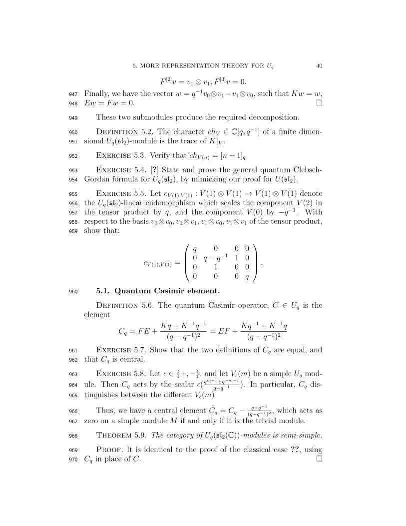
5. MORE REPRESENTATION THEORY FOR Uq 40

F [2]v = v1 ⊗ v1, F[3]v = 0.

Finally, we have the vector w = q−1v0⊗v1−v1⊗v0, such that Kw = w,947

Ew = Fw = 0. �948

These two submodules produce the required decomposition.949

Definition 5.2. The character chV ∈ C[q, q−1] of a finite dimen-950

sional Uq(sl2)-module is the trace of K|V .951

Exercise 5.3. Verify that chV (n) = [n + 1]q.952

Exercise 5.4. [?] State and prove the general quantum Clebsch-953

Gordan formula for Uq(sl2), by mimicking our proof for U(sl2).954

Exercise 5.5. Let cV (1),V (1) : V (1) ⊗ V (1) → V (1) ⊗ V (1) denote955

the Uq(sl2)-linear endomorphism which scales the component V (2) in956

the tensor product by q, and the component V (0) by −q−1. With957

respect to the basis v0⊗v0, v0⊗v1, v1⊗v0, v1⊗v1 of the tensor product,958

show that:959

cV (1),V (1) =

q 0 0 00 q − q−1 1 00 1 0 00 0 0 q

.

5.1. Quantum Casimir element.960

Definition 5.6. The quantum Casimir operator, C ∈ Uq is theelement

Cq = FE +Kq + K−1q−1

(q − q−1)2= EF +

Kq−1 + K−1q

(q − q−1)2

Exercise 5.7. Show that the two definitions of Cq are equal, and961

that Cq is central.962

Exercise 5.8. Let � ∈ {+,−}, and let V�(m) be a simple Uq mod-963

ule. Then Cq acts by the scalar �( qm+1+q−m−1

q−q−1 ). In particular, Cq dis-964

tinguishes between the different V�(m)965

Thus, we have a central element Cq = Cq − q+q−1

(q−q−1)2, which acts as966

zero on a simple module M if and only if it is the trivial module.967

Theorem 5.9. The category of Uq(sl2(C))-modules is semi-simple.968

Proof. It is identical to the proof of the classical case ??, using969

Cq in place of C. �970

6. THE LOCALLY FINITE PART AND THE CENTER OF Uq(sl2) 41

Remark 5.10. We have shown that when q is not a root of unity,971

the category of finite-dimensional type I Uq-modules is equivalent to972

the category U -mod, as abelian categories. However, as tensor cat-973

egories, they cannot be equivalent, because the co-product is non-974

cocommutative in Uq.975

Remark 5.11. For any M a finite dimensional Uq-module, we can976

decompose M = M+ ⊕ M−, where M+ is a sum of type I modules,977

M− is a sum of type II modules. Finally, we observe in passing that978

V−(m) ∼= V−(0)⊗ V+(m).979

6. The locally finite part and the center of Uq(sl2)980

There is a peculiarity in the construction of Uq(sl2). As with anyHopf algebra, we may consider the “adjoint” action of Uq(sl2) on itself:

x · y := x(1)yS(x(2)),

where Δ(x) = x(1) ⊗ x(2) (the implicit sum is suppressed in the nota-981

tion). In the classical setting, the adjoint action is just the commutator982

action, and we found (via the PBW theorem) that U(sl2) decomposed983

naturally as a direct sum of finite dimensional representations. In par-984

ticular, for any given x ∈ U(sl2), the orbit U(sl2) · x of x was finite-985

dimensional. For a Hopf algebra H, we let H � denote the sub-space of986

elements x which generate a finite orbit under the adjoint action.987

For Uq(sl2), we compute:

E · (ElKmF n)

= El+1KmF n −KElKmF nK−1E

= (1− q2l−2n+2m)El+1KmF n + q2l−2nElKm qn−1K − q1−nK−1

q − q−1[n]F n−1.

F · (ElKmF n)

= FElKmF nK − ElKmF nFK

= q2n(q−2m − q2)ElKm+1F n+1 − q2n[l]El−1Kqn−1 −K−1q1−n

q − q−1Km+1F n.

It follows easily that the locally finite part U �q(sl2) of Uq(sl2) is generated

by the elements EK−1, F,K−1. Let us define:

E = EK−1, F = F, K−1, L =1−K−2

q − q−1.

6. THE LOCALLY FINITE PART AND THE CENTER OF Uq(sl2) 42

We can easily compute commutation relations amonst generators ofU �(sl2):

EF − F E =1−K−2

q − q−1= L.(3)

q4LE − EL =q4E − q4K−2E − E + EK−2

q − q−1= q2[2]E.(4)

LF − q4F L =F −K−2F − q4F − q4FK−2

q − q−1= −q2[2]F .(5)

(q − q−1)L = 1−K−2.(6)

Proposition 6.1. The algebra U �q(sl2) is freely generated by E, F ,988

L, and K−1, subject to relations (3)-(6).989

Proposition 6.2. The specialization U �1(sl2), of U �

q(sl2) at q = 1,is isomorphic to U(sl2)⊗ C[Z/2], via:

φ : U �1(sl2)→ U(sl2)⊗ C[Z/2],

(E, F , L,K−1) �→ (E,F,H, �),

where � is the non-trivial element in Z/2.990

Proposition 6.3. We have an isomorphism,

U �q(sl2)

∼= C[Z/2]⊗��

k≥0

SymkqV (1)

�.

Corollary 6.4. The center of Uq(sl2) is the subalgebra freely gen-991

erated by Cq.992

Proof. The center of any Hopf algebra coincides with the ad-993

invariant part, and so is clearly contained in U �q. The character com-994

putation of Chapter 1 therefore applies mutatis mutandis. �995

CHAPTER 5

Categorical Commutativity in Braided Tensor996

Categories997

43

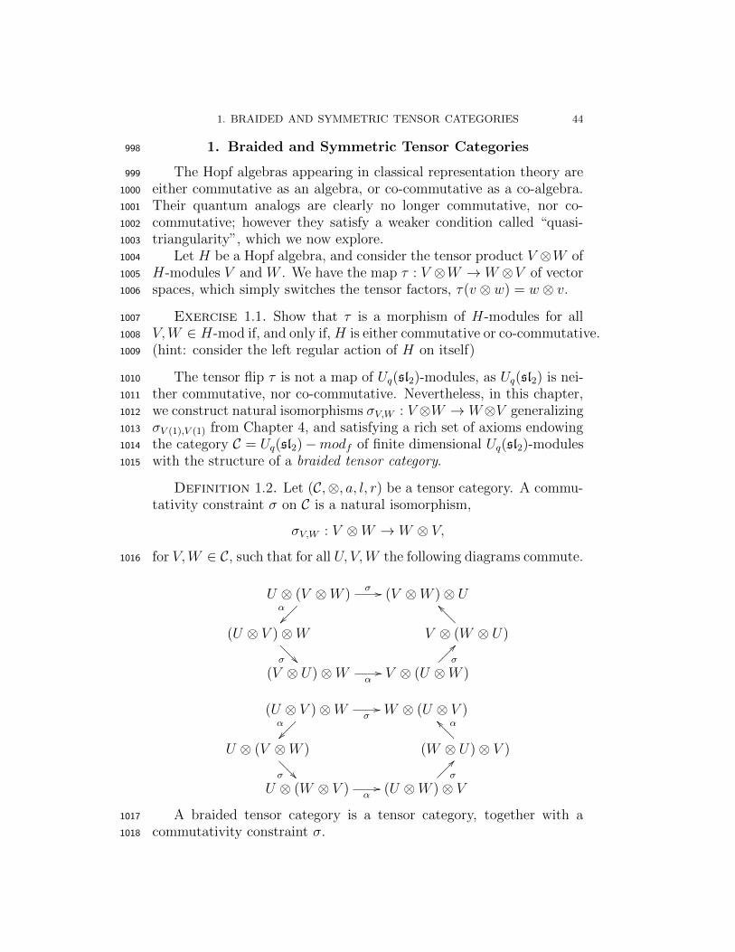
1. BRAIDED AND SYMMETRIC TENSOR CATEGORIES 44

1. Braided and Symmetric Tensor Categories998

The Hopf algebras appearing in classical representation theory are999

either commutative as an algebra, or co-commutative as a co-algebra.1000

Their quantum analogs are clearly no longer commutative, nor co-1001

commutative; however they satisfy a weaker condition called “quasi-1002

triangularity”, which we now explore.1003

Let H be a Hopf algebra, and consider the tensor product V ⊗W of1004

H-modules V and W . We have the map τ : V ⊗W → W ⊗V of vector1005

spaces, which simply switches the tensor factors, τ(v ⊗ w) = w ⊗ v.1006

Exercise 1.1. Show that τ is a morphism of H-modules for all1007

V,W ∈ H-mod if, and only if, H is either commutative or co-commutative.1008

(hint: consider the left regular action of H on itself)1009

The tensor flip τ is not a map of Uq(sl2)-modules, as Uq(sl2) is nei-1010

ther commutative, nor co-commutative. Nevertheless, in this chapter,1011

we construct natural isomorphisms σV,W : V ⊗W → W⊗V generalizing1012

σV (1),V (1) from Chapter 4, and satisfying a rich set of axioms endowing1013

the category C = Uq(sl2)−modf of finite dimensional Uq(sl2)-modules1014

with the structure of a braided tensor category.1015

Definition 1.2. Let (C,⊗, a, l, r) be a tensor category. A commu-tativity constraint σ on C is a natural isomorphism,

σV,W : V ⊗W → W ⊗ V,

for V,W ∈ C, such that for all U, V,W the following diagrams commute.1016

U ⊗ (V ⊗W )σ ��

α

������

(V ⊗W )⊗ U

(U ⊗ V )⊗W

σ �����

�V ⊗ (W ⊗ U)

������

(V ⊗ U)⊗W α�� V ⊗ (U ⊗W )

σ

������

(U ⊗ V )⊗W σ��

α

������

W ⊗ (U ⊗ V )

U ⊗ (V ⊗W )

σ �����

�(W ⊗ U)⊗ V )

�����

U ⊗ (W ⊗ V ) α�� (U ⊗W )⊗ V

σ

������

A braided tensor category is a tensor category, together with a1017

commutativity constraint σ.1018

1. BRAIDED AND SYMMETRIC TENSOR CATEGORIES 45

Remark 1.3. Like the pentagon axiom for the associator, the hexagon1019

axiom resolves a potential ambiguity. To move W past U ⊗V , one can1020

either group U and V , and commute W past them jointly, or pass1021

them one at a time. The hexagon diagram axiom asserts that in either1022

manner, you obtain the same isomorphism.1023

Remark 1.4. More concisely, a commutativity constraint is the1024

data necessary to equip the identity functor, Id : C → Cop, from C to the1025

category Cop with the structure of a tensor functor, where Cop denotes1026

the same underlying abelian category as C, but with V ⊗opW := W⊗V .1027

Proposition 1.5. Let C be a braided tensor category, and let U, V,W ∈C. Then (suppressing associators), we have the following equality inHomC(U ⊗ V ⊗W,W ⊗ V ⊗ U):

σV,W ◦ σU,W ◦ σU,V = σU,V σU,WσV,W .

Proof. The naturality of σ in each argument implies:

σV⊗U,W ◦ σV,W ⊗ IdW = σV,W ◦ σU⊗V,W .

Applying the hexagon axiom to each of σV⊗U,W and σU⊗V,W , we obtain1028

asserted equality. �1029

Definition 1.6. A braided tensor category C is symmetric if for1030

each V,W ∈ C, we have σV,W ◦ σW,V = Id.1031

Exercise 1.7. Let H be a commutative or co-commutative Hopf1032

algebra. Check that σ = τ is a commutativity constraint on H-mod,1033

and that it squares to the identity, so that H-mod is a symmetric tensor1034

category.1035

Exercise 1.8. Denote by Sn the symmetric group on n letters,1036

generated by adjacent swaps si,i+1. Let V ∈ C be an element of a1037

symmetric tensor category. Show that the map si,i+1 �→ Id. ⊗ · · · ⊗1038

σV,V ⊗· · ·⊗Id. defines a homomorphism of Sn to End(V ⊗n). In the case1039

C = H-mod, and dimC V ≥ n, show that this is an inclusion. (Hint:1040

consider a basis e1, . . . , en, and argue that the stabilizer of e1⊗· · ·⊗ en1041

is trivial).1042

When q is not a root of unity, we exhibited in Chapter ?? an1043

equivalence of abelian categories between the category of finite dimen-1044

sional type-I Uq(sl2)-modules and that of the finite dimensional U(sl2)-1045

modules. There we observed that as tensor categories these two are1046

not equivalent, because Uq(sl2) is non-cocommutative.1047

2. R-MATRIX PRELIMINARIES 46

2. R-matrix Preliminaries1048

In this section we answer the natural question: what is the necessarystructure on a Hopf algebra H, to endow C = H-mod with the structureof a braided tensor category? To answer this question, let us supposethat the category H-mod is braided, and consider the left regular actoinof H on itself. We have a braiding

σH,H : H ⊗H → H ⊗H.

We define R := τσH⊗H(1⊗ 1). Given arbitrary H-modules M and N ,and arbitrary elements m ∈ M ,n ∈ N , we have a homomorphism ofH-modules,

µm,n : H ⊗H →M ⊗N,

h1 ⊗ h2 �→ h1m⊗ h2n.

By naturality of σ, we must have σM,N(m⊗ n) = τR(m⊗ n).1049

Remark 2.1. For historical reasons relating to their physics origins,1050

braiding operators are often called R-matrices. Elements R ∈ H ⊗H1051

obtained in this way are called “universal R-matrices”, as their action1052

on any V ⊗W is an R-matrix.1053

Exercise 2.2. Show that the element R is invertible and satisfies1054

Δop(u) = RΔ(u)R−1, where Δop = τH,H ◦Δ, or in Sweedler’s notation,1055

Δop(u) = u(2) ⊗ u(1). Hint: Apply the H-linearity of cV,W1056

Exercise 2.3. Show that the hexagon relations imply the identity(Δ ⊗ id)(R) = R13R23 and (id ⊗ Δ)(R) = R13R12, where for R =�

si ⊗ ti, we define:

R13 :=�

si ⊗ 1⊗ ti, R23 :=�

1⊗ si ⊗ ti, R12 =�

si ⊗ ti ⊗ 1.

Definition 2.4. A quasi-triangular Hopf algebra is a Hopf algebra1057

H, equipped with an invertible element R ∈ H⊗H, such that Δop(u) =1058

RΔ(u)R−1 for all u ∈ H, and satisfying (Δ ⊗ id)(R) = R13R23 and1059

(id⊗Δ)(R) = R13R12.1060

Exercise 2.5. Let H be a quasi-triangular Hopf algebra, with H-modules M and N . Define H-module homomorphisms,

σM,N : M ⊗N → N ⊗M,

σ(m⊗ n) := τ(R(m⊗ n)).

Prove that σ defines a braiding on the category of H-modules.1061

We have shown that the data of a braiding on the category of H-1062

modules is equivalent to that of a quasi-triangular structure on H.1063

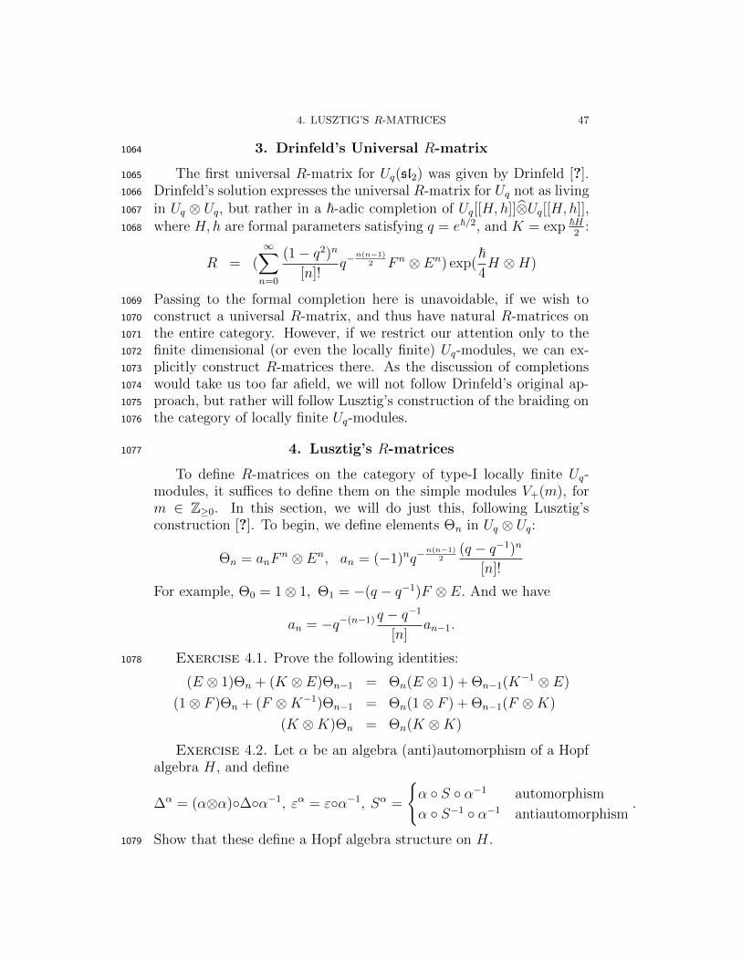
4. LUSZTIG’S R-MATRICES 47

3. Drinfeld’s Universal R-matrix1064

The first universal R-matrix for Uq(sl2) was given by Drinfeld [?].1065

Drinfeld’s solution expresses the universal R-matrix for Uq not as living1066

in Uq ⊗ Uq, but rather in a �-adic completion of Uq[[H, h]]�⊗Uq[[H, h]],1067

where H, h are formal parameters satisfying q = e�/2, and K = exp �H2

:1068

R = (∞�

n=0

(1− q2)n

[n]!q−

n(n−1)2 F n ⊗ En) exp(

�4H ⊗H)

Passing to the formal completion here is unavoidable, if we wish to1069

construct a universal R-matrix, and thus have natural R-matrices on1070

the entire category. However, if we restrict our attention only to the1071

finite dimensional (or even the locally finite) Uq-modules, we can ex-1072

plicitly construct R-matrices there. As the discussion of completions1073

would take us too far afield, we will not follow Drinfeld’s original ap-1074

proach, but rather will follow Lusztig’s construction of the braiding on1075

the category of locally finite Uq-modules.1076

4. Lusztig’s R-matrices1077

To define R-matrices on the category of type-I locally finite Uq-modules, it suffices to define them on the simple modules V+(m), form ∈ Z≥0. In this section, we will do just this, following Lusztig’sconstruction [?]. To begin, we define elements Θn in Uq ⊗ Uq:

Θn = anFn ⊗ En, an = (−1)nq−

n(n−1)2

(q − q−1)n

[n]!

For example, Θ0 = 1⊗ 1, Θ1 = −(q − q−1)F ⊗ E. And we have

an = −q−(n−1) q − q−1

[n]an−1.

Exercise 4.1. Prove the following identities:1078

(E ⊗ 1)Θn + (K ⊗ E)Θn−1 = Θn(E ⊗ 1) + Θn−1(K−1 ⊗ E)

(1⊗ F )Θn + (F ⊗K−1)Θn−1 = Θn(1⊗ F ) + Θn−1(F ⊗K)

(K ⊗K)Θn = Θn(K ⊗K)

Exercise 4.2. Let α be an algebra (anti)automorphism of a Hopfalgebra H, and define

Δα = (α⊗α)◦Δ◦α−1, εα = ε◦α−1, Sα =

�α ◦ S ◦ α−1 automorphism

α ◦ S−1 ◦ α−1 antiautomorphism.

Show that these define a Hopf algebra structure on H.1079

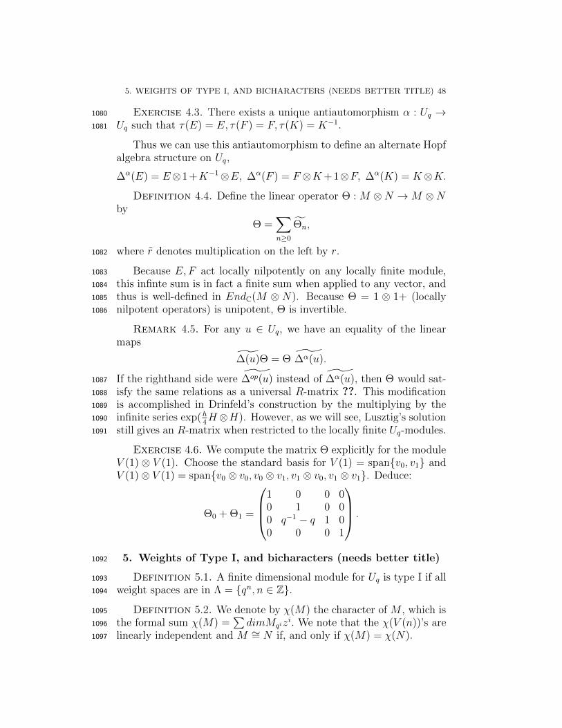
5. WEIGHTS OF TYPE I, AND BICHARACTERS (NEEDS BETTER TITLE) 48

Exercise 4.3. There exists a unique antiautomorphism α : Uq →1080

Uq such that τ(E) = E, τ(F ) = F, τ(K) = K−1.1081

Thus we can use this antiautomorphism to define an alternate Hopfalgebra structure on Uq,

Δα(E) = E⊗1+K−1⊗E, Δα(F ) = F ⊗K+1⊗F, Δα(K) = K⊗K.

Definition 4.4. Define the linear operator Θ : M ⊗N →M ⊗Nby

Θ =�

n≥0

�Θn,

where r denotes multiplication on the left by r.1082

Because E,F act locally nilpotently on any locally finite module,1083

this infinte sum is in fact a finite sum when applied to any vector, and1084

thus is well-defined in EndC(M ⊗ N). Because Θ = 1 ⊗ 1+ (locally1085

nilpotent operators) is unipotent, Θ is invertible.1086

Remark 4.5. For any u ∈ Uq, we have an equality of the linearmaps

�Δ(u)Θ = Θ �Δα(u).

If the righthand side were �Δop(u) instead of �Δα(u), then Θ would sat-1087

isfy the same relations as a universal R-matrix ??. This modification1088

is accomplished in Drinfeld’s construction by the multiplying by the1089

infinite series exp(h4H⊗H). However, as we will see, Lusztig’s solution1090

still gives an R-matrix when restricted to the locally finite Uq-modules.1091

Exercise 4.6. We compute the matrix Θ explicitly for the moduleV (1) ⊗ V (1). Choose the standard basis for V (1) = span{v0, v1} andV (1)⊗ V (1) = span{v0 ⊗ v0, v0 ⊗ v1, v1 ⊗ v0, v1 ⊗ v1}. Deduce:

Θ0 + Θ1 =

1 0 0 00 1 0 00 q−1 − q 1 00 0 0 1

.

5. Weights of Type I, and bicharacters (needs better title)1092

Definition 5.1. A finite dimensional module for Uq is type I if all1093

weight spaces are in Λ = {qn, n ∈ Z}.1094

Definition 5.2. We denote by χ(M) the character of M , which is1095

the formal sum χ(M) =�

dimMqizi. We note that the χ(V (n))’s are1096

linearly independent and M ∼= N if, and only if χ(M) = χ(N).1097

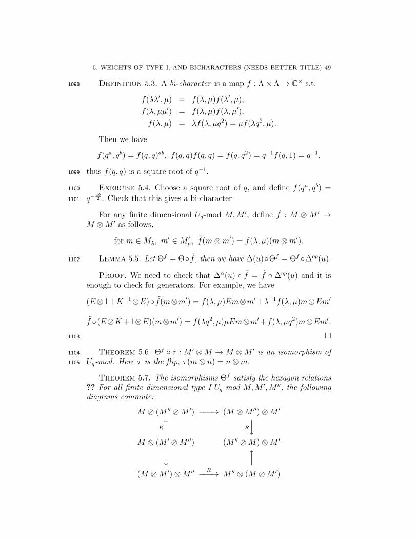
5. WEIGHTS OF TYPE I, AND BICHARACTERS (NEEDS BETTER TITLE) 49

Definition 5.3. A bi-character is a map f : Λ× Λ→ C× s.t.1098

f(λλ�, µ) = f(λ, µ)f(λ�, µ),

f(λ, µµ�) = f(λ, µ)f(λ, µ�),

f(λ, µ) = λf(λ, µq2) = µf(λq2, µ).

Then we have

f(qa, qb) = f(q, q)ab, f(q, q)f(q, q) = f(q, q2) = q−1f(q, 1) = q−1,

thus f(q, q) is a square root of q−1.1099

Exercise 5.4. Choose a square root of q, and define f(qa, qb) =1100

q−ab2 . Check that this gives a bi-character1101

For any finite dimensional Uq-mod M,M �, define f : M ⊗M � →M ⊗M � as follows,

for m ∈Mλ, m� ∈M �µ, f(m⊗m�) = f(λ, µ)(m⊗m�).

Lemma 5.5. Let Θf = Θ◦ f , then we have Δ(u)◦Θf = Θf ◦Δop(u).1102

Proof. We need to check that Δα(u) ◦ f = f ◦ Δop(u) and it isenough to check for generators. For example, we have

(E⊗1+K−1⊗E)◦ f(m⊗m�) = f(λ, µ)Em⊗m�+λ−1f(λ, µ)m⊗Em�

f ◦(E⊗K+1⊗E)(m⊗m�) = f(λq2, µ)µEm⊗m�+f(λ, µq2)m⊗Em�.

�1103

Theorem 5.6. Θf ◦ τ : M � ⊗M → M ⊗M � is an isomorphism of1104

Uq-mod. Here τ is the flip, τ(m⊗ n) = n⊗m.1105

Theorem 5.7. The isomorphisms Θf satisfy the hexagon relations?? For all finite dimensional type I Uq-mod M,M �,M ��, the followingdiagrams commute:

M ⊗ (M �� ⊗M �) −−−→ (M ⊗M ��)⊗M �

R

� R

�M ⊗ (M � ⊗M ��) (M �� ⊗M)⊗M �

��

(M ⊗M �)⊗M �� R−−−→ M �� ⊗ (M ⊗M �)

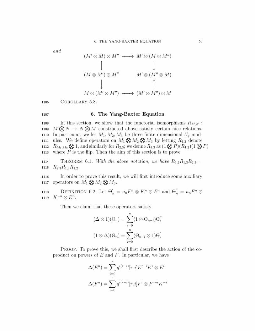
6. THE YANG-BAXTER EQUATION 50

and(M � ⊗M)⊗M �� −−−→ M � ⊗ (M ⊗M ��)�

�(M ⊗M �)⊗M �� M � ⊗ (M �� ⊗M)�

�M ⊗ (M � ⊗M ��) −−−→ (M � ⊗M ��)⊗M

Corollary 5.8.1106

6. The Yang-Baxter Equation1107

In this section, we show that the functorial isomorphisms RM,N :1108

M�

N → N�

M constructed above satisfy certain nice relations.1109

In particular, we let M1,M2,M3 be three finite dimensional Uq mod-1110

ules. We define operators on M1

�M2

�M3 by letting R1,2 denote1111

RM1,M2

�1, and similarly for R2,3; we define R1,3 as (1

�P )(R1,2)(1

�P )1112

where P is the flip. Then the aim of this section is to prove1113

Theorem 6.1. With the above notation, we have R1,2R1,3R2,3 =1114

R2,3R1,3R1,2.1115

In order to prove this result, we will first introduce some auxiliary1116

operators on M1

�M2

�M3.1117

Definition 6.2. Let Θ�n = anF

n ⊗ Kn ⊗ En and Θ��n = anF

n ⊗1118

K−n ⊗ En.1119

Then we claim that these operators satisfy

(Δ⊗ 1)(Θn) =n�

i=0

(1⊗Θn−i)Θ��i

(1⊗Δ)(Θn) =n�

i=0

(Θn−i ⊗ 1)Θ�i

Proof. To prove this, we shall first describe the action of the co-product on powers of E and F . In particular, we have

Δ(En) =r�

i=0

qi(r−i)[r i]Er−iK i ⊗ Ei

Δ(F n) =r�

i=0

qi(r−i)[r i]F i ⊗ F r−iK−i

6. THE YANG-BAXTER EQUATION 51

where we use [n i] to denote the quantum binomial coefficient. Theproof of these identities goes by induction, the case r = 1 being thedefinition of the coproduct. To see the first identity in general:

Δ(En) = Δ(E)Δ(En−1)

= (E ⊗ 1 + K ⊗ E)(r−1�

i=0

qi(r−1−i)[(r − 1) i]Er−1−iK i ⊗ Ei)

=r−1�

i=0

qi(r−1−i)[(r − 1) i]Er−iK i ⊗ Ei +r�

i=1

q(i−1)(r−1)[(r − 1) (i− 1)]KEr−iK i−1 ⊗ Ei

=r−1�

i=0

qi(r−1−i)[(r − 1) i]Er−iK i ⊗ Ei +r�

i=1

q(i+1)(r−1)[(r − 1) (i− 1)]Er−iK i ⊗ Ei

=r�

i=0

qi(r−i)(q−i[(r − 1) i] + qr−i[(r − 1) (i− 1)])Er−iK i ⊗ Ej

So we have reduced the question to showing (q−i[(r − 1) i] + qr−i[(r −1) (i− 1)]) = [r i] which is an easy consequence of the definition. Theformula for F is proved by the same considerations. Now, we knowthat (Δ⊗1)(Θn) = an(Δ(F n)⊗En). Applying the above formula thenyields

n�

j=0

(q−j(n−j))[n j](an)Fj ⊗K−jF n−j ⊗ En

On the other side, computing�n

i=0(1 ⊗ Θn−i)Θ��i immediately yields1120 �n

j=0(an−jaj)(Fj⊗F n−jK−j⊗En) which is equal to

�nj=0(an−jaj)(q

−2j(n−j))(F j⊗1121

K−jF n−j ⊗En). So we see that it suffices to show (q−2j(n−j))ajan−j =1122

(q−j(n−j))[n j](an), but this is an easy computation from the definitions.1123

The second formula follows from similar computations. �1124

Now, the proof of the main theorem uses formulas obtained from theabove via twisting by τ , where τ is the antiautomorphism of Uq whichpreserves E and F and sends K to K−1. Then we have (τ ⊗ τ)(Θn) =Θn, while (τ ⊗ τ ⊗ τ)(Θ

�n) = Θ

��n. Applying (τ ⊗ τ ⊗ τ) to the above

equations thus yields

(τΔ⊗ 1)(Θn) =n�

i=0

Θ�i(1⊗Θn−i)

(1⊗τΔ)(Θn) =n�

i=0

Θ��i (Θn−i ⊗ 1)

6. THE YANG-BAXTER EQUATION 52

We shall also need several more identities: if we define f1,2 to be f ⊗ 1

(and similarly for f2,3 and f1,3), then we have the relations f1,2Θ1,3 =

Θ�f1,2 and f2,3Θ1,3 = Θ

��f2,3, where Θ

�=

�n Θ

�n and similarly for Θ

��;

these relations follow immediately from the multiplicative properties off . Further, one also easily derives

f1,2f2,3(1⊗Θ) = (1⊗Θ)f1,2f2,3

f2,3f1,3(Θ⊗ 1) = (Θ⊗ 1)f2,3f1,3

To conclude that the Yang-Baxter equation holds, we write out bothsides; the left hand being

(Θ⊗ 1)f1,2Θ1,3f1,3(1⊗Θ)f2,3

and the right hand being

(1⊗Θ)f2,3Θ1,3f1,3(Θ⊗ 1)f1,2

Now, using the above relations to rearrange the left hand side, one gets

(Θ⊗ 1)(Θ�)(1⊗Θ)f1,3f1,2f2,3

To deal with this, we rearrange the Θ terms as follows:

(Θ⊗ 1)(Θ�)(1⊗Θ)

=�

n,i

(Θ⊗ 1)(Θ�i)(1⊗Θn−i)

=�

n

(Θ⊗ 1)(τΔ⊗ 1)(Θn)

=�

n

(Δ⊗ 1)(Θn)(Θ⊗ 1)

=�

n,i

(1⊗Θn−i)(Θ��i )(Θ⊗ 1)

= (1⊗Θ)(Θ��)(Θ⊗ 1)

Where the third equality follows from the definition of Θ and the co-1125

product. But this expression composed with f1,3f1,2f2,3 is precisely the1126

right hand side; as is easily seen by using the above relations (and1127

noting that the f ’s all commute).1128

7. THE HEXAGON DIAGRAMS 53

7. The hexagon Diagrams1129

Theorem 7.1. The following diagrams commute:

M ⊗ (M� ⊗M

��)

1⊗R−−−→ M ⊗ (M�� ⊗M

�)

can−−−→ (M ⊗M��)⊗M

� R⊗1−−−→ (M�� ⊗M)⊗M

�

=

� =

�

M ⊗ (M� ⊗M

��)

can−−−→ (M ⊗M�)⊗M

�� R−−−→ M�� ⊗ (M ⊗M

�)

can−−−→ (M�� ⊗M)⊗M

�

and also

(M ⊗M�)⊗M

�� R⊗1−−−→ (M� ⊗M)⊗M

�� can−−−→ M� ⊗ (M ⊗M

��)

1⊗R−−−→ M� ⊗ (M

�� ⊗M)

=

� =

�

(M ⊗M�)⊗M

�� can−−−→ M ⊗ (M� ⊗M

��)

R−−−→ (M� ⊗M

��)⊗M

can−−−→ M� ⊗ (M

�� ⊗M)

Proof. We shall prove the bottom diagram, the proof of the topis almost the same. In the top part of this diagram, the first R isΘ1,2f1,2P1,2 while the second R is Θ2,3f2,3P2,3. Therefore, we considerthe composition, which is

Θ2,3f2,3P2,3Θ1,2f1,2P1,2

= Θ2,3f2,3Θ1,3P2,3f1,2P1,2

= Θ2,3f2,3Θ1,3f1,3P2,3P1,2

= Θ2,3Θ��f2,3f1,3P2,3P1,2

where we have used the following equalities: P2,3Θ1,2 = Θ1,3P2,3 and1130

P2,3f1,2 = f1,3P2,3 and f2,3Θ1,3 = Θ��f2,3. The last one was proved in1131

the previous section, while the first two are immediate consequences of1132

the definitions. Now, the lower half of the diagram involves only one1133

R, which is given by the permutation (132) = (23)(12), followed by1134

the diagonal matrix f(λµ, ν) (on a weight vector in Mλ ⊗Mµ ⊗Mν),1135

followed by (Δ⊗ 1)(Θ) (as the action on the tensor product is defined1136

by Δ). But we also have (Δ ⊗ 1)(Θ) = (Θ2,3)(Θ��), so combining this1137

with the relation f(λµ, ν) = f(λ, ν)f(µ, ν) shows that the two halves1138

of the diagram are equal. �1139

CHAPTER 6

Geometric Representation Theory for SLq(2)1140

54

2. GENERATORS AND RELATIONS FOR Oq 55

1. The Quantum Group Algebra1141

In this section, we provide two independent constructions of a Hopf1142

algebra Oq(SL2), which plays the role of the coordinate algebra O(SL2)1143

in the quantum setting. First, we construct Oq(SL2) as the algebra of1144

matrix coefficients associated to Uq(sl2), as in Chapter 2. Secondly,1145

we introduce a simple non-commutative algebra called the quantum1146

plane, and construct an algebra show that Oq(Mat2), the universal1147

bi-algebra co-acting on the quantum plane, and inside there exhibit a1148

central “q-determinant”, which we may set to one, to obtain Oq(SL2).1149

Definition 1.1. The quantized coordinate algebra, Oq(SL(2)),1150

henceforth denoted Oq, is the subspace of U ∗q spanned by matrix co-1151

efficients of type I representations, i.e., linear functionals of the form1152

cf,v(u) := f(uv), for V a type I representation of Uq, f ∈ V ∗, v ∈ V .1153

That Oq is a subalgebra follows immediately from the formulacf,ecf �,e� = cf⊗f �,e⊗e� (as in the classical case). We give Oq a coalge-bra structure via Δ(cfi,ej) =

�k cfi,ek ⊗ cfk,ej . An antipode is obtained

from that on Uq, via the bi-linear pairing between Uq and Oq: fora ∈ Oq, we define S(a) by the formula:

�S(a), x� = �a, S(x)�,where x ∈ Uq is arbitrary. That this makes Oq into a Hopf algebra is1154

an easy verification, just as in the classical case.1155

2. Generators and Relations for Oq1156

Inspecting the proof of the Peter-Weyl Theorem for classical SL2,1157

we see that the proof hinged only on the fact that the category of1158

Uq(sl2)-modules is semi-simple, and that we had an explicit list of all1159

simple objects. The category of finite-dimensional Uq(sl2)-modules is1160

also semi-simple, and its simple objects are in bijection with those of1161

U(sl2). Thus we have:1162

Proposition 2.1. There exists an isomorphism of Uq(sl2)⊗Uq(sl2)-modules,

Oq∼=

�

k

V ∗(k) � V (k).

Remark 2.2. There is one subtlety in the construction of Oq: by1163

design the algebra O(SL2) was equivariant for U(sl2) ⊗ U(sl2). We1164

should expect the same for Oq, that it be equivariant for the action1165

of Uq ⊗ Uq. However, there is a catch, which is that the antipode1166

S : Uq → Uq is an anti-automorphism of the coproduct, i.e. Δ(S(x)) =1167

2. GENERATORS AND RELATIONS FOR Oq 56

S(x(2)) ⊗ S(x(1)). This means that Oq is natural an algebra in the1168

category Cop�C, not C�C. This is merely a reflection of contravariance1169

of the duality functor ∗ : C → C.1170

We wish to derive a “generators and relations” presentation of Oq,1171

from its definition as matrix coefficients. To begin, we note that, as1172

before, the module V (1) generates all finite dimensional representations1173

in the sense that V (n) ⊂ V (1)⊗n (as follows from Clebsch-Gordan).1174

Letting C�a, b, c, d� denote the free algebra on symbols a, b, c, d, wehave a surjection,

C�a, b, c, d�� Oq,

(a, b, c, d) �→ (cf0,v0 , cf1,v0 , cf0,v1 , cf1,v1).

Now, we can use the R-matrix to compute the commutativity relationsbetween the matrix coefficients of V (1), which we label a, b, c, d, wherea = c0,0, b = c0,1, c = c1,0 and d = c1,1. We label the R-matrix entries

Rk,li,j and these are given by

cV,V (vi ⊗ vj) =�

Rk,li,jvl ⊗ vk.

Then we recall from the previous lecture that we have

R0,00,0 = R1,1

1,1 = q−1, R1,00,1 = R0,1

1,0 = 1, R1,01,0 = q − q−1,

and all remaining entries zero. These coefficients imply the following1175

Lemma 2.3. The generators a, b, c, d satisfy the following relations:

ab = qba, bc = cb, cd = qdc, ac = qca,

bd = qdb, ad− da = (q − q−1)bc, ad− qbc = 1.

Proof. Each of the purely quadratic relations is obtained by ap-plying the relations,�

Rijkla

kmaln =

�Rijklcf l⊗fk,vm⊗vn = cσ∗(f i⊗fj),vm⊗vn

= cf i⊗fj ,σ(vm⊗vn) =�

cf i⊗fj ,vs⊗vtRtsmn =

�ajsa

itR

tsmn,

the so-called Fadeev-Reshetikhin-Takhtajian (FRT) relations.1176

For instance,

qba = qc0,1c0,0 = qcf0⊗f0,v1⊗v0 = cσ∗(f0⊗f0),v1⊗v0= cf0⊗f0,c(v1⊗v0) = cf0⊗f0,v0⊗v1 = c0,0c0,1 = ab

ad = c0,0c1,1 = cf1⊗f0,v0⊗v1 = cσ∗(f0⊗f1),v0⊗v1

= cf0⊗f1,σ(v0⊗v1) = cf0⊗f1,v1⊗v0 + (q − q−1)cf0⊗f1,v0⊗v1

= c1,1c0,0 + (q − q−1)c1,0c0,1 = da + (q − q−1)cb.

3. Oq COMODULES 57

The remaining quadratic relations are proved similarly. The determi-1177

nant relation follows, as in the classical SL2 computation. �1178

Exercise 2.4. Using the PBW theorem for Oq(SL2), show that1179

the above generators and relations yield a presentation of Oq. (Hint:1180

all the ingredients of Exercise ??) can be applied mutatis mutandis to1181

the quantum setting.1182

With this isomorphism in hand, we can explicitly exhibit the Hopf1183

algebra structure on Oq. The comultiplication is given by Δ{a, b, c, d} =1184

{a, b, c, d} ⊗ {a, b, c, d} where the right hand side symbolizes matrix1185

multiplication; this is immediate from the above presentation of Oq.1186

The antipode is given by S({a, b, c, d}) = {d, qb,−q−1c, a}; one checks1187

easily that this is an antipode on SLq(2), and then we know from gen-1188

eral Hopf algebra theory that if an antipode exists, it is unique; so it1189

coincides with the antipode given by the pairing with Uq.1190

3. Oq comodules1191

Let M be a right Oq-comodule. Then we can put a left Uq-module1192

structure on M as follows: by definition there is a map Δ : M →1193

M ⊗ Oq. Therefore we have maps Uq ⊗M → Uq ⊗M ⊗ Oq → M ⊗1194

Uq ⊗ Oq → M where the second to last map is the flip and the last1195

is 1⊗ <,>. By the properties of the Hopf pairing, this map makes1196

M into a left U module. In particular, this association is a functor1197

from right Oq comodules to left Uq modules, which, when restricted to1198

finite dimensional M , yields only type 1 Uq modules. This is because1199

the weights of K on M are given by coefficients of eigenvectors coming1200

from expressions of the form < K, o > for o ∈ Oq; but the collection1201

of these is {qn}n∈Z as Oq is defined using only type 1 modules. Our1202

remaining aim in this lecture is to show1203

Theorem 3.1. The functor from finite dimensional right Oq co-1204

modules to type 1 finite dimensional left Uq modules is an equivalence1205

of categories.1206

Proof. In general, suppose C is a coalgebra and M a finite dimen-1207

sional comodule. Let {m1, ...,mn} be a basis for M . Then we can write1208

the coaction as Δmi =�

j mj⊗cj,i. Now, coassociativity of this action1209

tells us that it is the same to apply ΔM ⊗1 and 1⊗ΔC . The first gives1210 �j,k mk ⊗ ck,j ⊗ cj,i, and so this implies that Δci,j =

�j ck,j ⊗ cj,i, or,1211

in matrix notation, Δ(cr,m) = (cr,m)⊗ (cr,m). Further, from the counit1212

axiom, �ci,j = δi,j . Now, if you are given a collection of n2 elements1213

of C called (ci,j), whose counit and comultiplication satisfy the above1214