Slides 4: The New Keynesian Model

(following Galí 2007)

Bianca De Paoli

November 2009

1 The New Keynesian Model

� widely used for monetary policy analysis

� framework that can help us understand the links between monetary policyand the aggregate performance of an economy:

� understand how interest rate decisions end up a¤ecting the variousmeasures of an economy�s performance, i.e. the transmission mecha-nism of monetary policy

� understand what should be the objectives of monetary policy and howthe latter should be conducted in order to attain those objectives

� RBC model - perfect competition, frictionless markets and no monetarysector

� Classical monetary model - money is neutral and the Friedman rule isoptimal

� Money neutrality: monetary policy (ie changes in money supply ornominal interest rates) have no e¤ect on real variables.

� Friedman rule: the opportunity cost of holding money faced by pri-vate agents should equal the social cost of creating additional �atmoney)Thus nominal rates of interest should be zero.

� In practice, this means that the central bank should seek a rate ofde�ation equal to the real interest rate on government bonds and othersafe assets, in order to make the nominal interest rate zero.

� But at odds with

� empirical evidence (money has short run real e¤ects)

� and monetary policy practice (rates are not kept at zero)

� The canonical New Keynesian model: RBC model, usually abstracting fromcapital accumulation, with some non-classical features

1.1 Key elements in a New Keynesian model

� Monopolistic competition: The prices of goods and inputs are set byprivate economic agents in order to maximize their objectives, as opposedto being determined by an anonymous Walrasian auctioneer seeking toclear all (competitive) markets at once.

� Nominal rigidities: Firms are subject to some constraints on the frequencywith which they can adjust the prices of the goods and services they sell(Calvo price setting). Alternatively, �rms may face some costs of adjustingthose prices (Rotemberg price setting). The same kind of friction appliesto workers in the presence of sticky wages.

� Short run non-neutrality of monetary policy: As a consequence of thepresence of nominal rigidities, changes in short term nominal interest rates(whether chosen directly by the central bank or induced by changes inthe money supply) lead to variations in real interest rates (given that realmoney balances and expected in�ation do not move proportionally).

� The latter bring about changes in consumption and investment

� and since �rms �nd it optimal to adjust the quantity of goods supplied tothe new level of demand, output and employment also change

� In the long run, however, all prices and wages adjust, and the economyreverts back to its natural equilibrium.

� We will use Gali�s book and lecture notes

� First, let�s revise the classical model with and without money in the utility

� Then introduce monopolistic competition and nominal rigidities - the canon-ical NK model

1.2 Classical model - Recalling the RBC model but ab-

stracting from capital

Households

Representative household solves

maxU(Ct;Nt)

or

maxUt = Et

1Xs=t

�s�t24C1��s

1� �� N

1+'s

1 + '

35 ;subject to

CtPt +QtBt � Bt�1 +WtNt � Tt

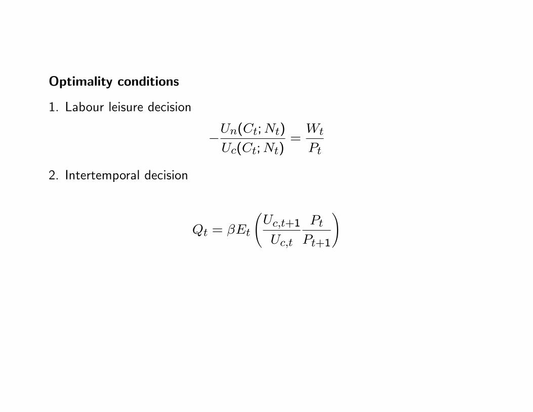
Optimality conditions

1. Labour leisure decision

�Un(Ct;Nt)Uc(Ct;Nt)

=Wt

Pt

2. Intertemporal decision

Qt = �Et

Uc;t+1

Uc;t

Pt

Pt+1

!

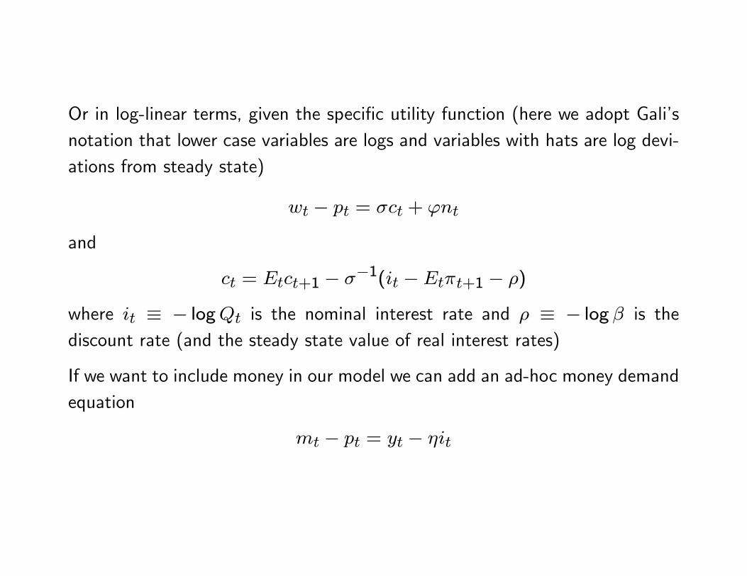
Or in log-linear terms, given the speci�c utility function (here we adopt Gali�snotation that lower case variables are logs and variables with hats are log devi-ations from steady state)

wt � pt = �ct + 'nt

and

ct = Etct+1 � ��1(it � Et�t+1 � �)

where it � � logQt is the nominal interest rate and � � � log � is thediscount rate (and the steady state value of real interest rates)

If we want to include money in our model we can add an ad-hoc money demandequation

mt � pt = yt � �it

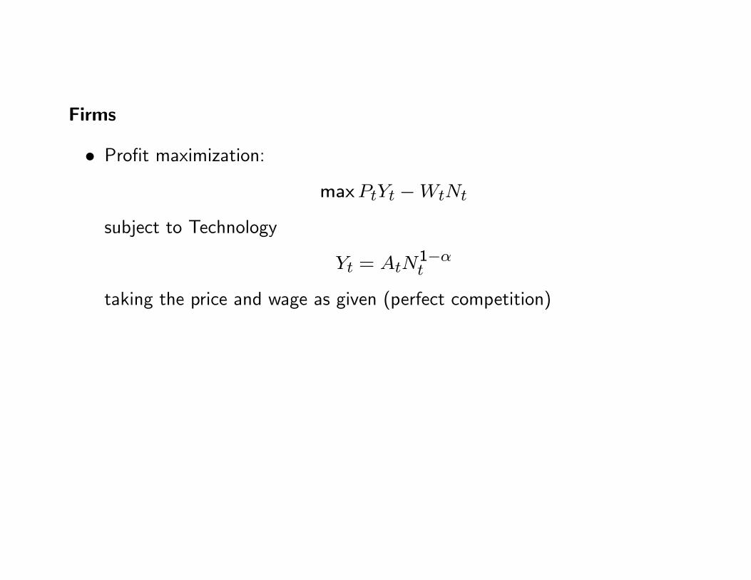
Firms

� Pro�t maximization:

maxPtYt �WtNt

subject to Technology

Yt = AtN1��t

taking the price and wage as given (perfect competition)

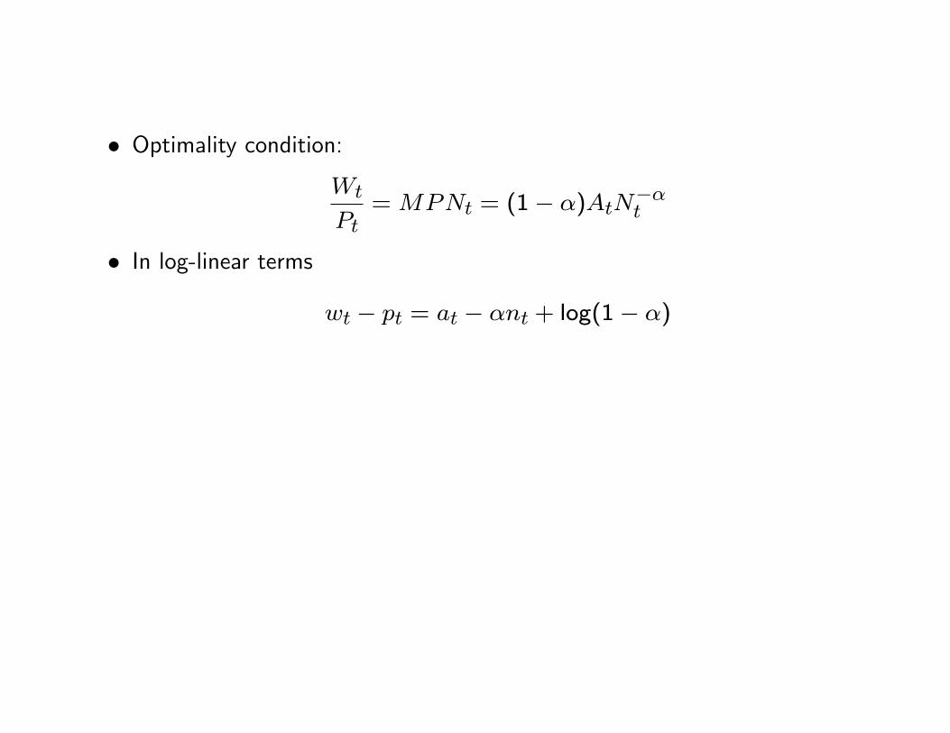
� Optimality condition:Wt

Pt=MPNt = (1� �)AtN

��t

� In log-linear terms

wt � pt = at � �nt + log(1� �)

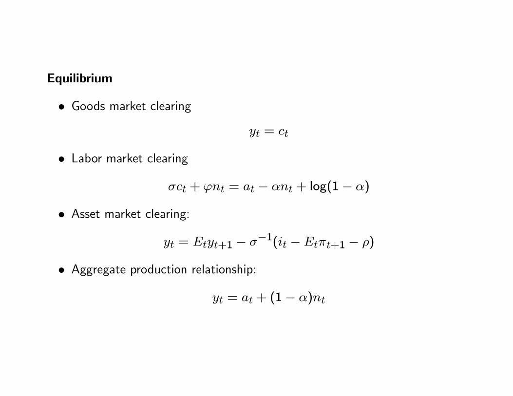
Equilibrium

� Goods market clearing

yt = ct

� Labor market clearing

�ct + 'nt = at � �nt + log(1� �)

� Asset market clearing:

yt = Etyt+1 � ��1(it � Et�t+1 � �)

� Aggregate production relationship:

yt = at + (1� �)nt

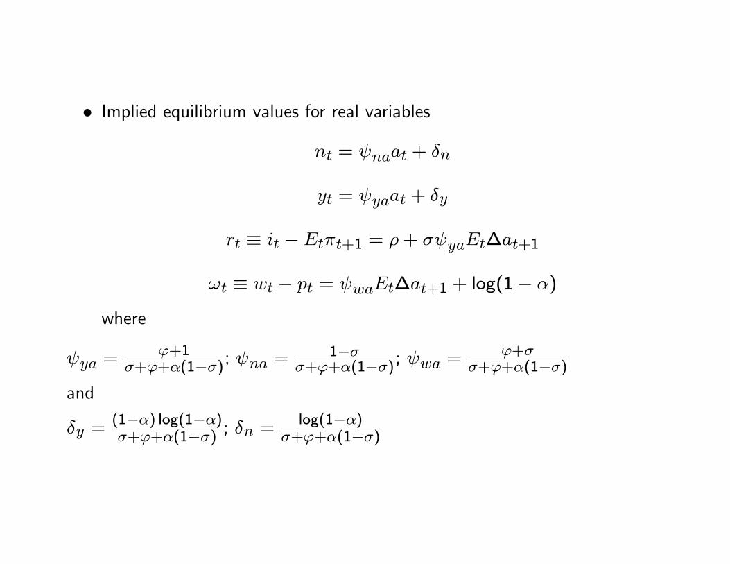
� Implied equilibrium values for real variables

nt = naat + �n

yt = yaat + �y

rt � it � Et�t+1 = �+ � yaEt�at+1

!t � wt � pt = waEt�at+1 + log(1� �)

where

ya ='+1

�+'+�(1��); na =1��

�+'+�(1��); wa ='+�

�+'+�(1��)

and

�y =(1��) log(1��)�+'+�(1��) ; �n =

log(1��)�+'+�(1��)

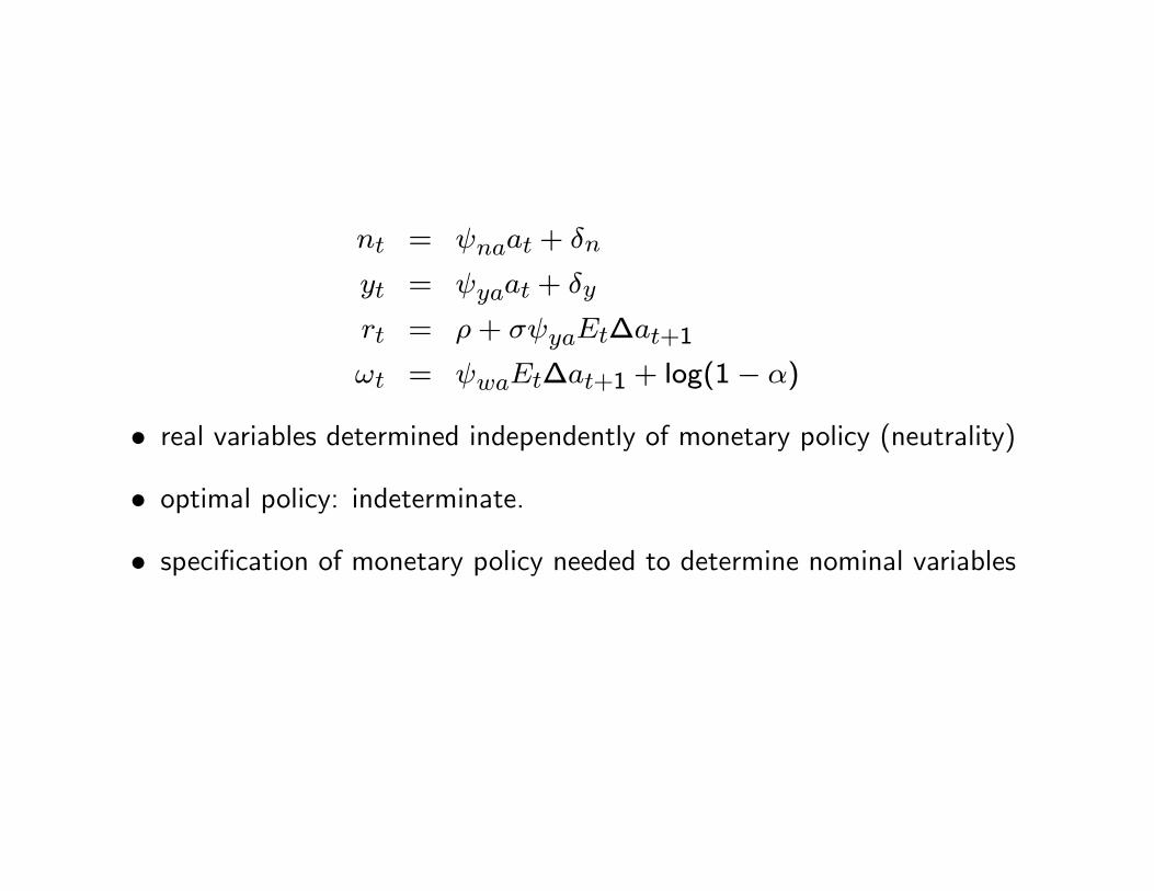
nt = naat + �n

yt = yaat + �y

rt = �+ � yaEt�at+1

!t = waEt�at+1 + log(1� �)

� real variables determined independently of monetary policy (neutrality)

� optimal policy: indeterminate.

� speci�cation of monetary policy needed to determine nominal variables

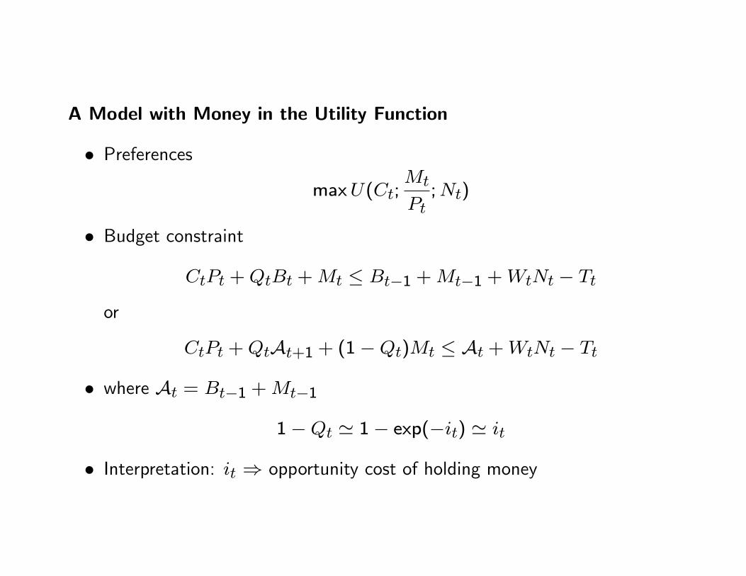
A Model with Money in the Utility Function

� Preferences

maxU(Ct;Mt

Pt;Nt)

� Budget constraint

CtPt +QtBt +Mt � Bt�1 +Mt�1 +WtNt � Tt

or

CtPt +QtAt+1 + (1�Qt)Mt � At +WtNt � Tt

� where At = Bt�1 +Mt�1

1�Qt ' 1� exp(�it) ' it

� Interpretation: it ) opportunity cost of holding money

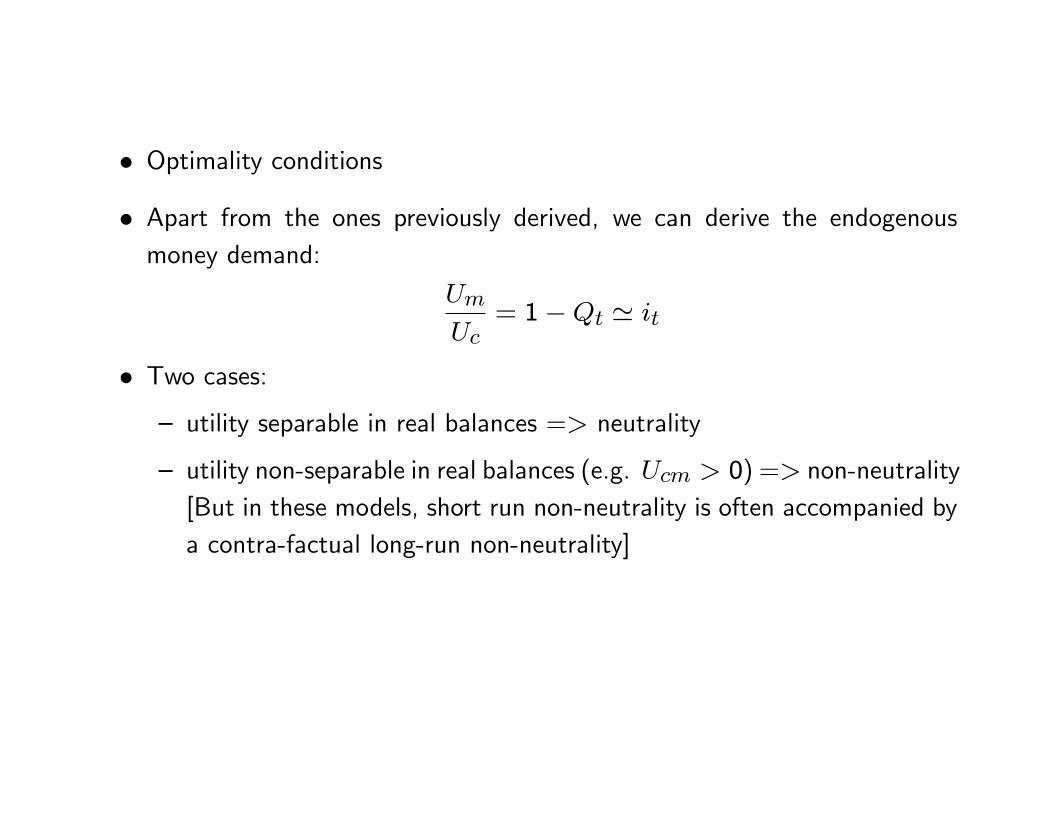
� Optimality conditions

� Apart from the ones previously derived, we can derive the endogenousmoney demand:

Um

Uc= 1�Qt ' it

� Two cases:

� utility separable in real balances => neutrality

� utility non-separable in real balances (e.g. Ucm > 0) => non-neutrality[But in these models, short run non-neutrality is often accompanied bya contra-factual long-run non-neutrality]

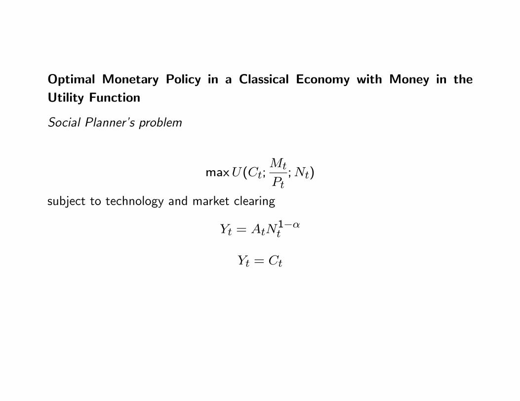
Optimal Monetary Policy in a Classical Economy with Money in theUtility Function

Social Planner�s problem

maxU(Ct;Mt

Pt;Nt)

subject to technology and market clearing

Yt = AtN1��t

Yt = Ct

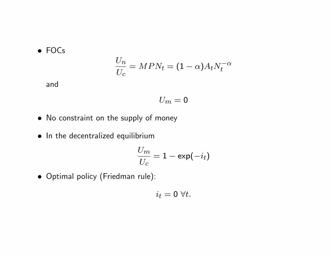
� FOCsUn

Uc=MPNt = (1� �)AtN

��t

and

Um = 0

� No constraint on the supply of money

� In the decentralized equilibriumUm

Uc= 1� exp(�it)

� Optimal policy (Friedman rule):

it = 0 8t:

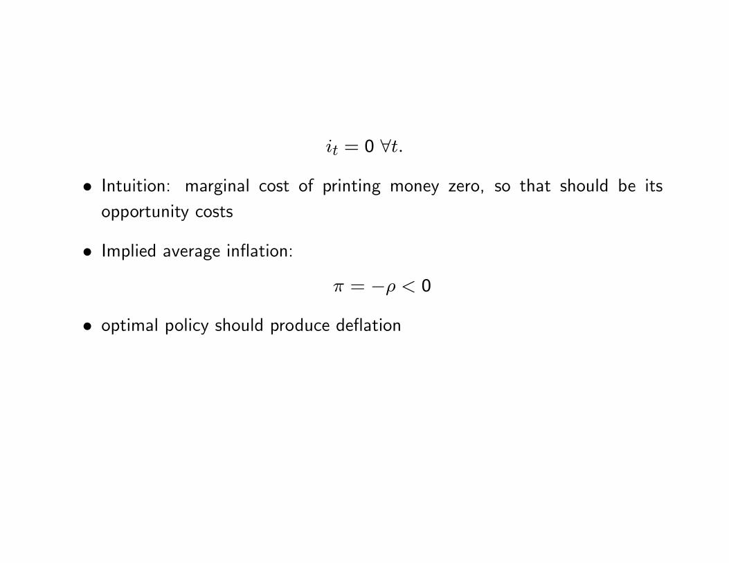
it = 0 8t:

� Intuition: marginal cost of printing money zero, so that should be itsopportunity costs

� Implied average in�ation:

� = �� < 0

� optimal policy should produce de�ation

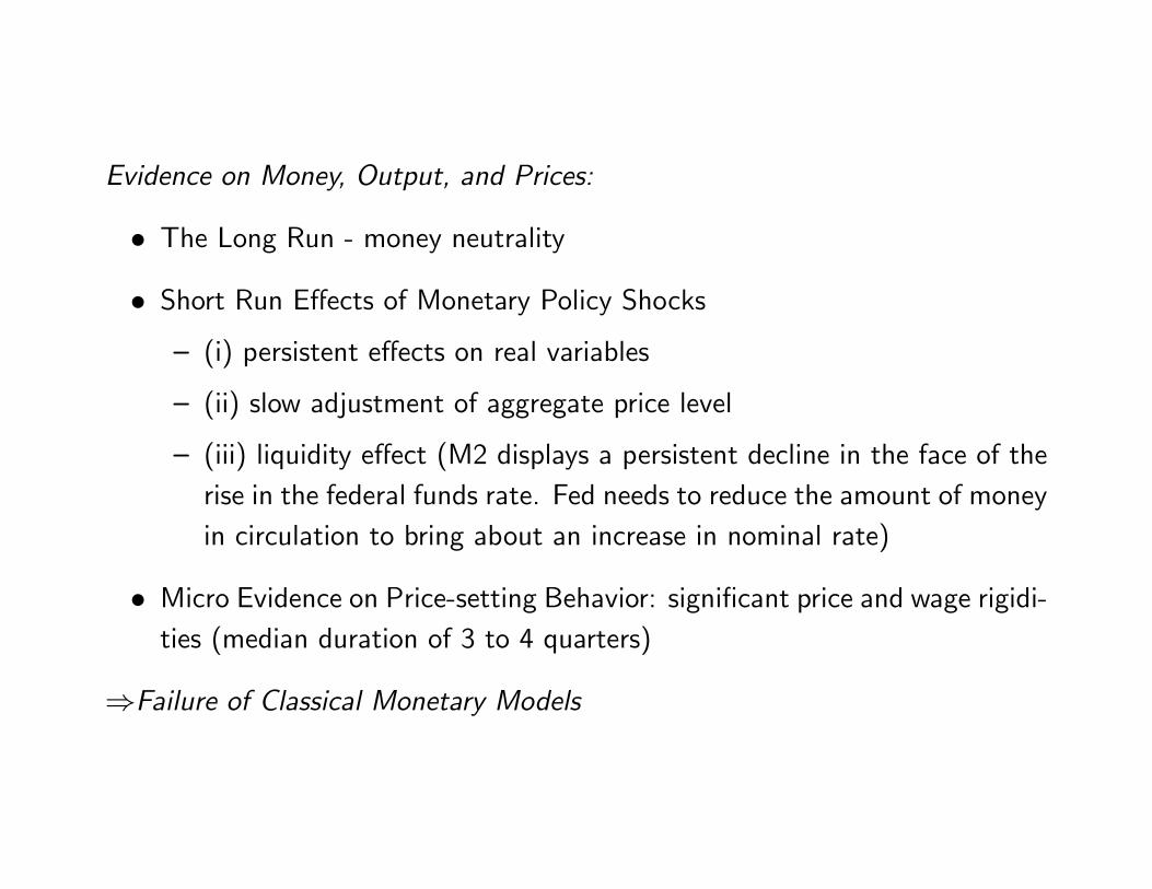
Evidence on Money, Output, and Prices:

� The Long Run - money neutrality

� Short Run E¤ects of Monetary Policy Shocks

� (i) persistent e¤ects on real variables

� (ii) slow adjustment of aggregate price level

� (iii) liquidity e¤ect (M2 displays a persistent decline in the face of therise in the federal funds rate. Fed needs to reduce the amount of moneyin circulation to bring about an increase in nominal rate)

� Micro Evidence on Price-setting Behavior: signi�cant price and wage rigidi-ties (median duration of 3 to 4 quarters)

)Failure of Classical Monetary Models

� A Baseline Model with Nominal Rigidities

� monopolistic competition

� sticky prices (staggered price setting)

� competitive labor markets, closed economy, no capital accumulation

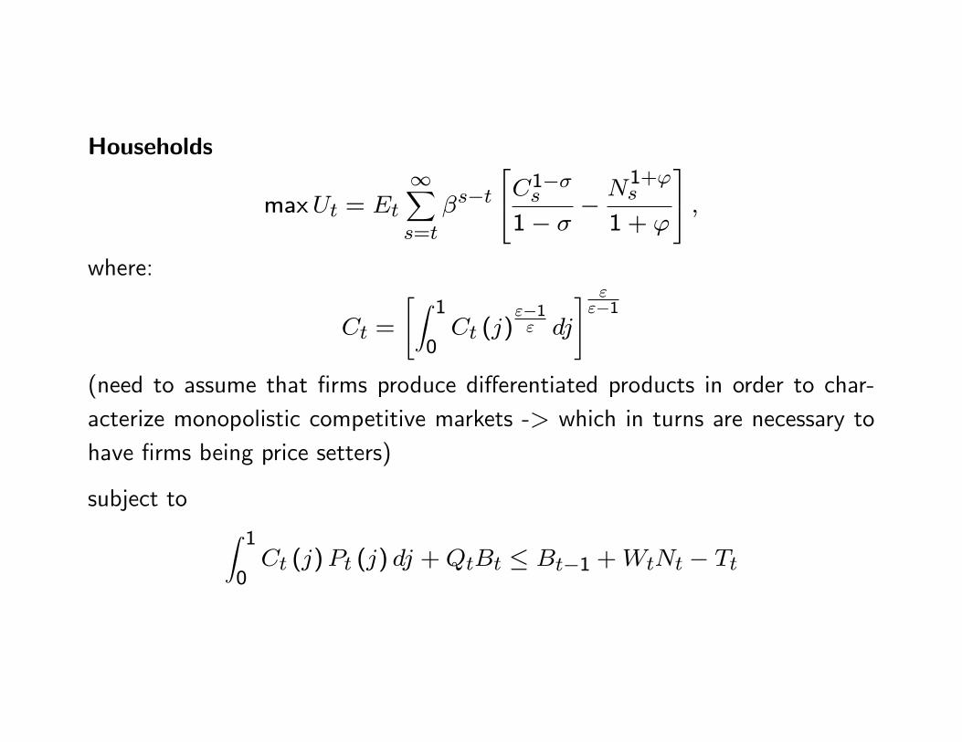
Households

maxUt = Et

1Xs=t

�s�t24C1��s

1� �� N

1+'s

1 + '

35 ;where:

Ct =

"Z 10Ct (j)

"�1" dj

# ""�1

(need to assume that �rms produce di¤erentiated products in order to char-acterize monopolistic competitive markets -> which in turns are necessary tohave �rms being price setters)

subject to Z 10Ct (j)Pt (j) dj +QtBt � Bt�1 +WtNt � Tt

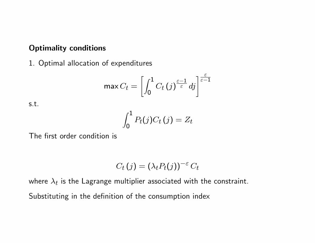
Optimality conditions

1. Optimal allocation of expenditures

maxCt =

"Z 10Ct (j)

"�1" dj

# ""�1

s.t. Z 10Pt(j)Ct (j) = Zt

The �rst order condition is

Ct (j) = (�tPt(j))�"Ct

where �t is the Lagrange multiplier associated with the constraint.

Substituting in the de�nition of the consumption index

�t =

"Z 10Pt(j)

1�"dj

# �11�"

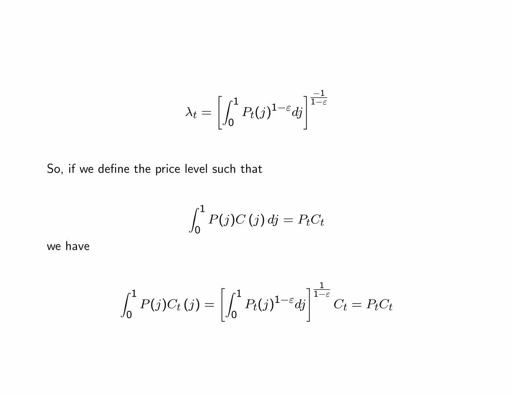
So, if we de�ne the price level such that

Z 10P (j)C (j) dj = PtCt

we have

Z 10P (j)Ct (j) =

"Z 10Pt(j)

1�"dj

# 11�"

Ct = PtCt

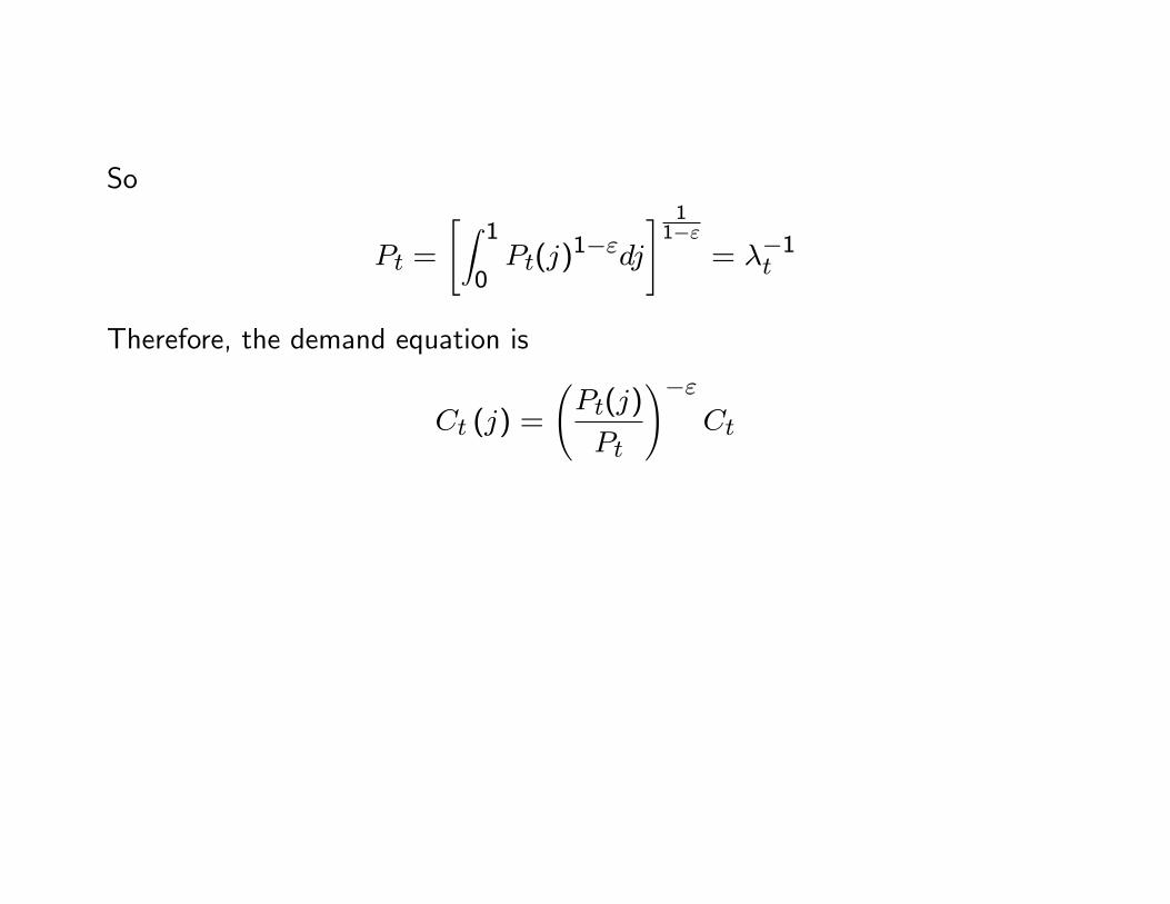
So

Pt =

"Z 10Pt(j)

1�"dj

# 11�"

= ��1t

Therefore, the demand equation is

Ct (j) =

Pt(j)

Pt

!�"Ct

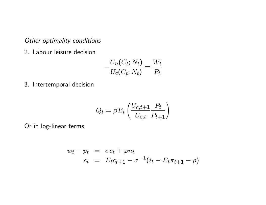
Other optimality conditions

2. Labour leisure decision

�Un(Ct;Nt)Uc(Ct;Nt)

=Wt

Pt

3. Intertemporal decision

Qt = �Et

Uc;t+1

Uc;t

Pt

Pt+1

!Or in log-linear terms

wt � pt = �ct + 'nt

ct = Etct+1 � ��1(it � Et�t+1 � �)

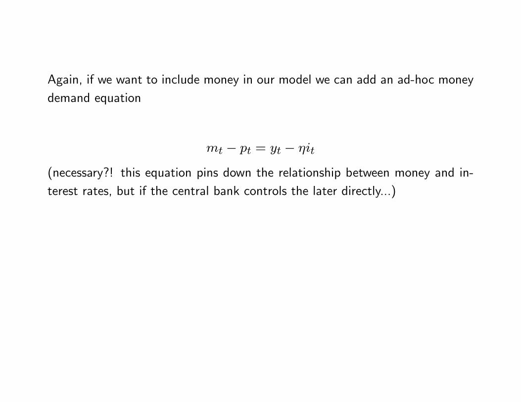
Again, if we want to include money in our model we can add an ad-hoc moneydemand equation

mt � pt = yt � �it

(necessary?! this equation pins down the relationship between money and in-terest rates, but if the central bank controls the later directly...)

Firms

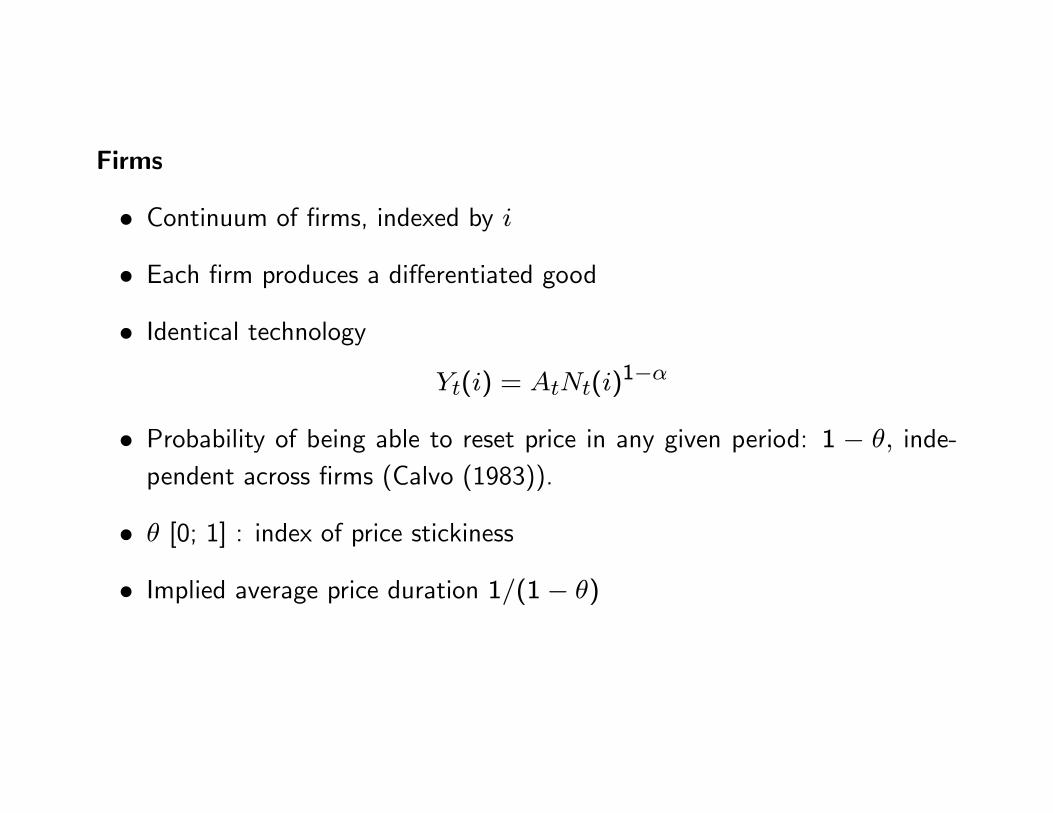
� Continuum of �rms, indexed by i

� Each �rm produces a di¤erentiated good

� Identical technology

Yt(i) = AtNt(i)1��

� Probability of being able to reset price in any given period: 1 � �; inde-pendent across �rms (Calvo (1983)).

� � [0; 1] : index of price stickiness

� Implied average price duration 1=(1� �)

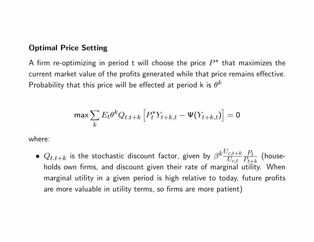
Optimal Price Setting

A �rm re-optimizing in period t will choose the price P � that maximizes thecurrent market value of the pro�ts generated while that price remains e¤ective.Probability that this price will be e¤ected at period k is �k

maxXk

Et�kQt:t+k

hP �t Yt+k;t �(Yt+k;t)

i= 0

where:

� Qt:t+k is the stochastic discount factor, given by �kUc;t+kUc;t

PtPt+k

(house-holds own �rms, and discount given their rate of marginal utility. Whenmarginal utility in a given period is high relative to today, future pro�tsare more valuable in utility terms, so �rms are more patient)

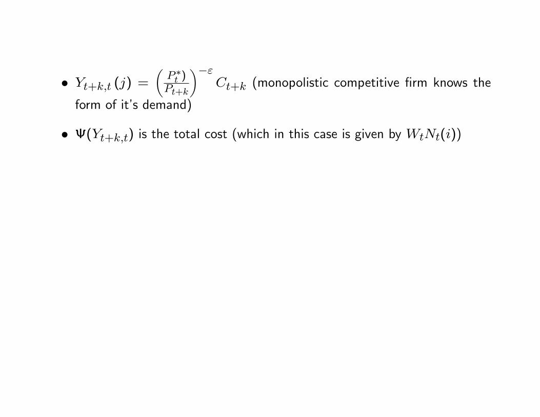
� Yt+k;t (j) =�P �t )Pt+k

��"Ct+k (monopolistic competitive �rm knows the

form of it�s demand)

� (Yt+k;t) is the total cost (which in this case is given by WtNt(i))

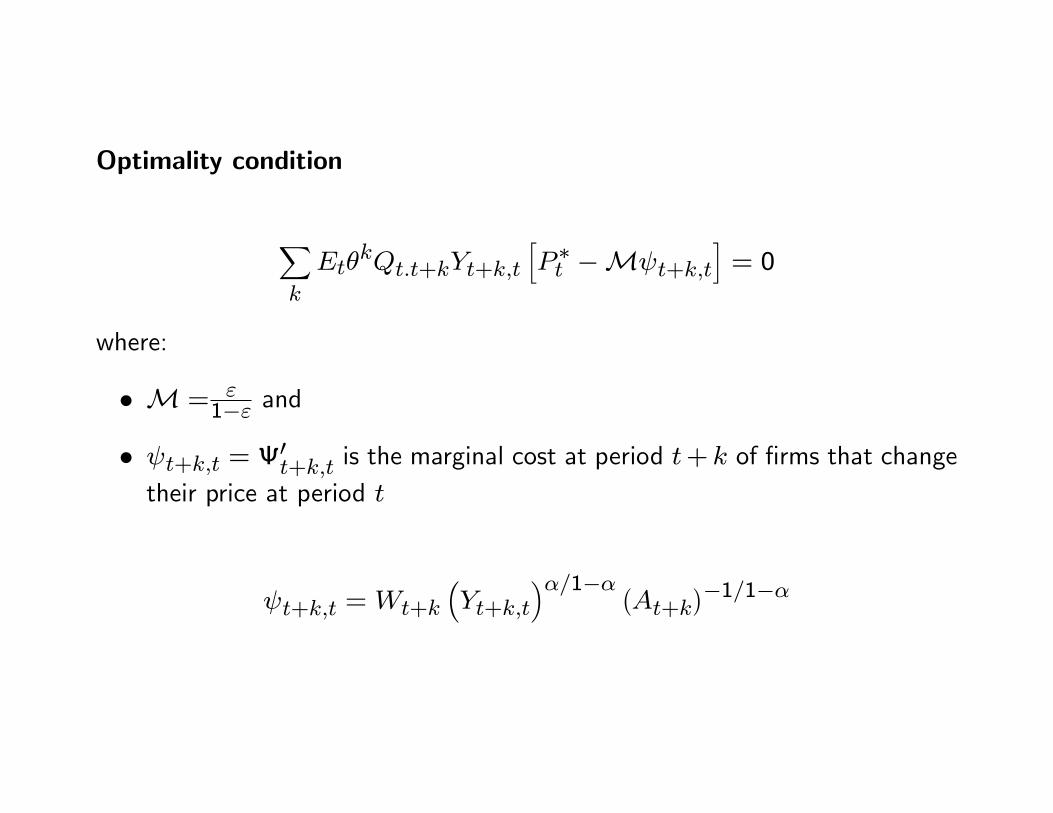
Optimality condition

Xk

Et�kQt:t+kYt+k;t

hP �t �M t+k;t

i= 0

where:

� M = "1�" and

� t+k;t = 0t+k;t is the marginal cost at period t+ k of �rms that changetheir price at period t

t+k;t =Wt+k

�Yt+k;t

��=1�� �At+k

��1=1��

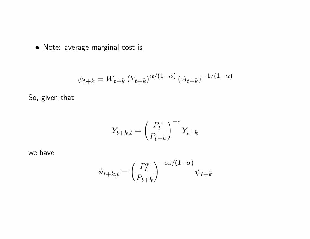
� Note: average marginal cost is

t+k =Wt+k�Yt+k

��=(1��) �At+k��1=(1��)So, given that

Yt+k;t =

P �tPt+k

!��Yt+k

we have

t+k;t =

P �tPt+k

!���=(1��) t+k

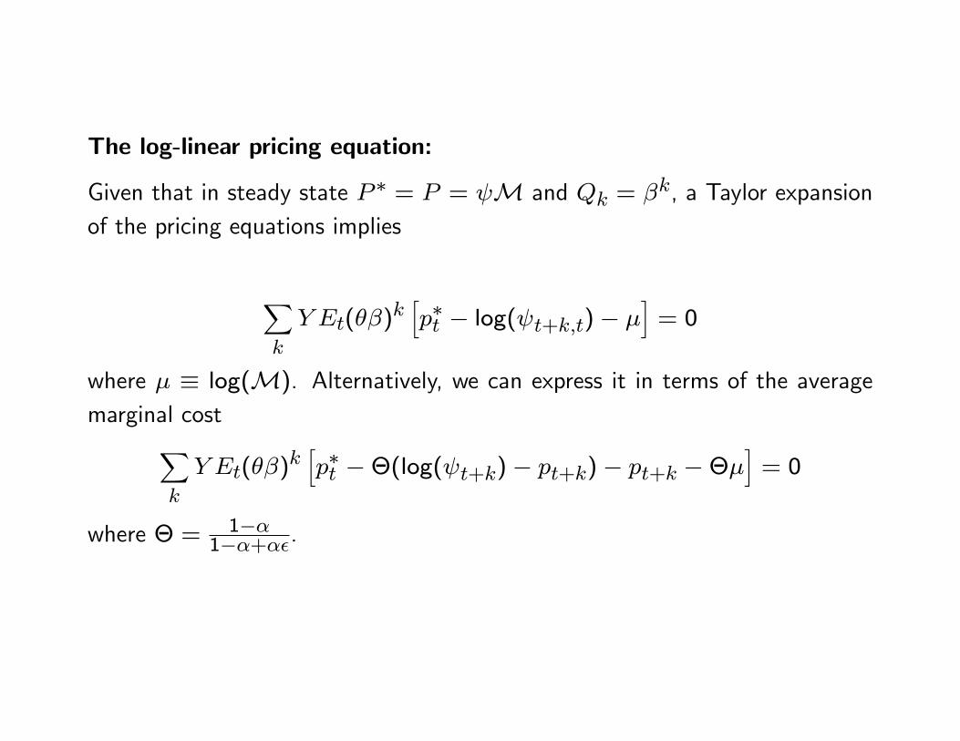
The log-linear pricing equation:

Given that in steady state P � = P = M and Qk = �k, a Taylor expansionof the pricing equations implies

Xk

Y Et(��)khp�t � log( t+k;t)� �

i= 0

where � � log(M). Alternatively, we can express it in terms of the averagemarginal costX

k

Y Et(��)khp�t ��(log( t+k)� pt+k)� pt+k ���

i= 0

where � = 1��1��+��.

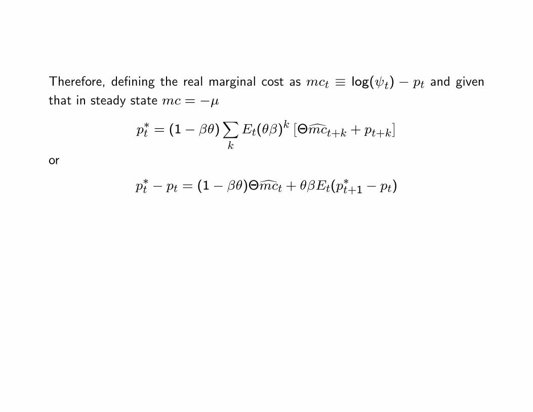
Therefore, de�ning the real marginal cost as mct � log( t) � pt and giventhat in steady state mc = ��

p�t = (1� ��)Xk

Et(��)k ��dmct+k + pt+k

�or

p�t � pt = (1� ��)�dmct + ��Et(p�t+1 � pt)

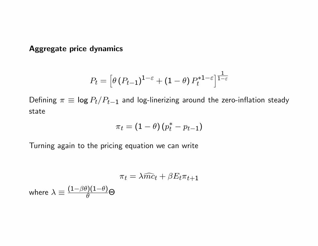
Aggregate price dynamics

Pt =h� (Pt�1)

1�" + (1� �)P �1�"t

i 11�"

De�ning � � logPt=Pt�1 and log-linerizing around the zero-in�ation steadystate

�t = (1� �) (p�t � pt�1)

Turning again to the pricing equation we can write

�t = �dmct + �Et�t+1

where � � (1���)(1��)� �

The log linear Phillips curve

In order to write the above pricing equation in terms of output, we need toderive some conditions for the real marginal cost and market clearing

� Goods market clearing

yt = ct

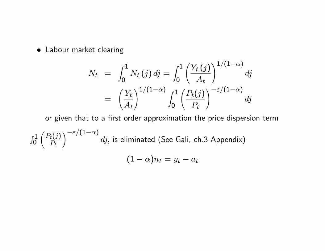
� Labour market clearing

Nt =Z 10Nt (j) dj =

Z 10

Yt (j)

At

!1=(1��)dj

=

Yt

At

!1=(1��) Z 10

Pt(j)

Pt

!�"=(1��)dj

or given that to a �rst order approximation the price dispersion term

R 10

�Pt(j)Pt

��"=(1��)dj; is eliminated (See Gali, ch.3 Appendix)

(1� �)nt = yt � at

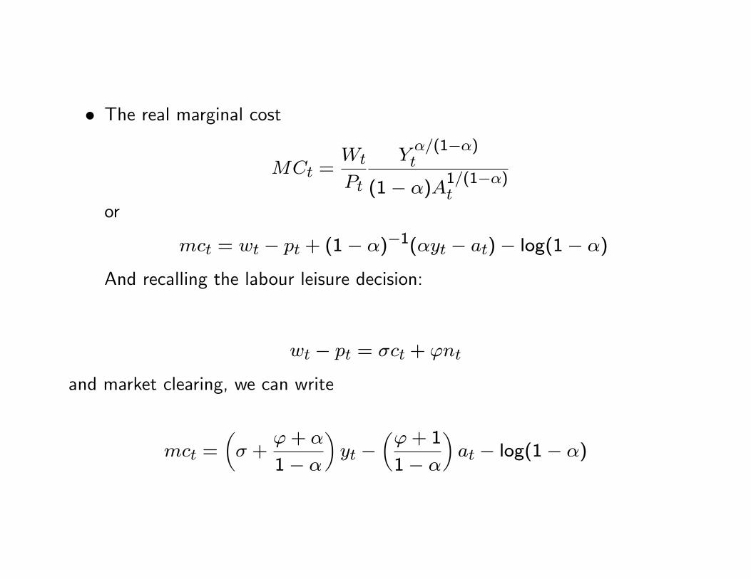
� The real marginal cost

MCt =Wt

Pt

Y�=(1��)t

(1� �)A1=(1��)t

or

mct = wt � pt + (1� �)�1(�yt � at)� log(1� �)

And recalling the labour leisure decision:

wt � pt = �ct + 'nt

and market clearing, we can write

mct =�� +

'+ �

1� �

�yt �

�'+ 1

1� �

�at � log(1� �)

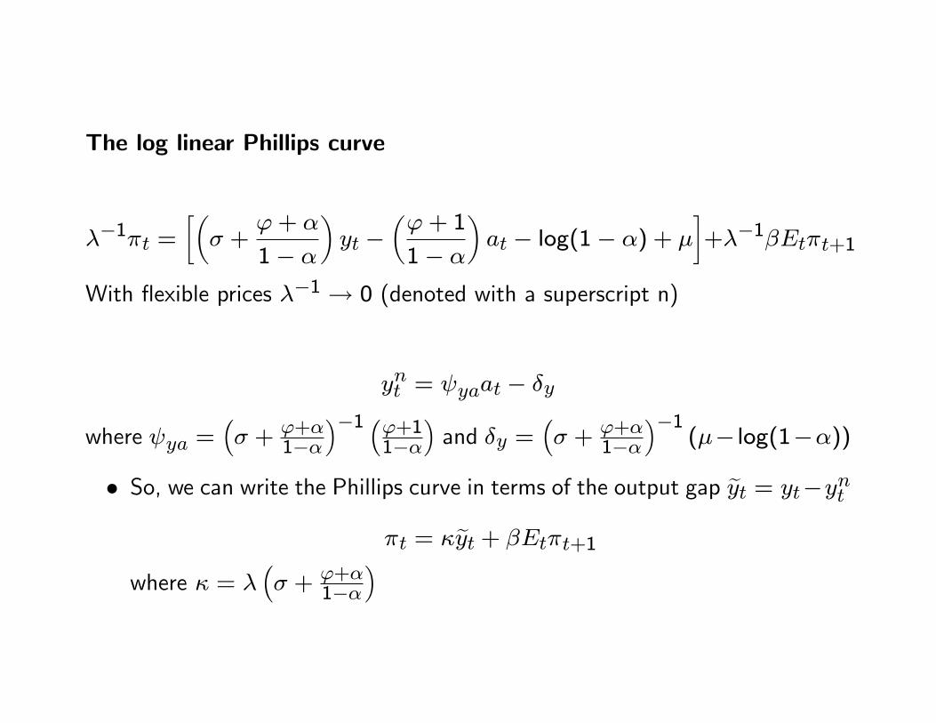
The log linear Phillips curve

��1�t =��� +

'+ �

1� �

�yt �

�'+ 1

1� �

�at � log(1� �) + �

�+��1�Et�t+1

With �exible prices ��1 ! 0 (denoted with a superscript n)

ynt = yaat � �y

where ya =�� + '+�

1����1 �'+1

1���and �y =

�� + '+�

1����1

(�� log(1��))

� So, we can write the Phillips curve in terms of the output gap eyt = yt�ynt

�t = �eyt + �Et�t+1

where � = ��� + '+�

1���

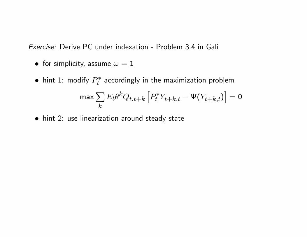
Exercise: Derive PC under indexation - Problem 3.4 in Gali

� for simplicity, assume ! = 1

� hint 1: modify P �t accordingly in the maximization problem

maxXk

Et�kQt:t+k

hP �t Yt+k;t �(Yt+k;t)

i= 0

� hint 2: use linearization around steady state

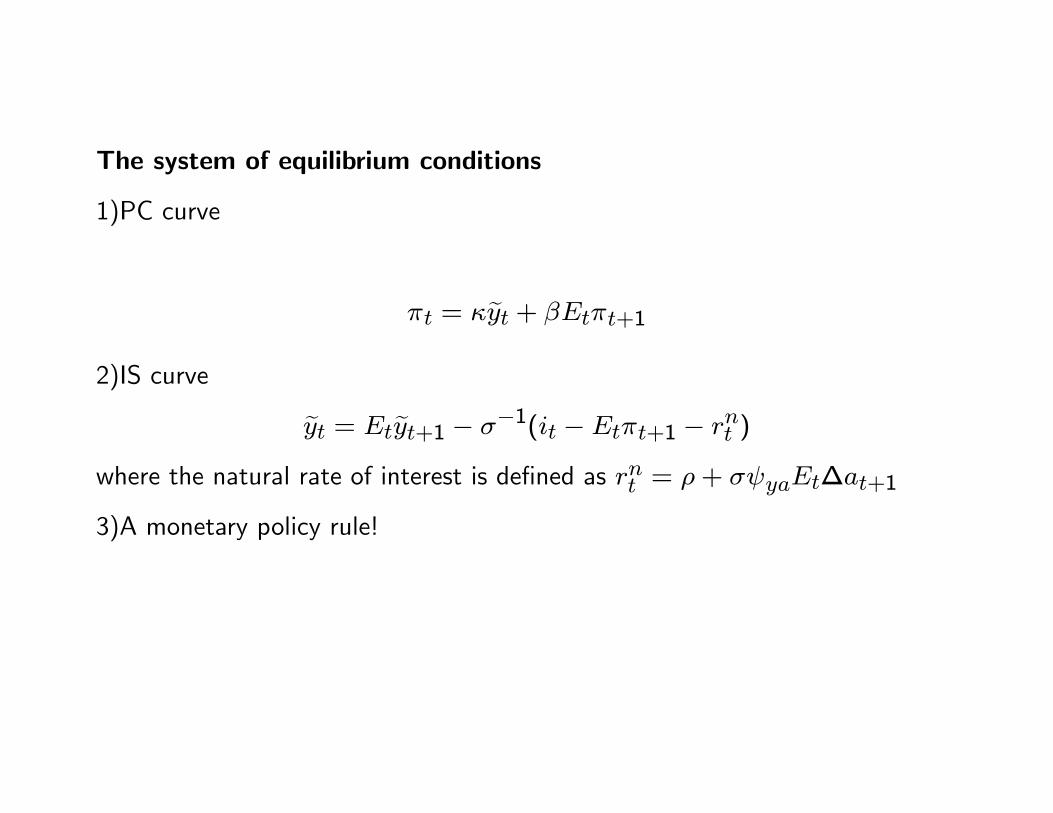
The system of equilibrium conditions

1)PC curve

�t = �eyt + �Et�t+1

2)IS curve

eyt = Eteyt+1 � ��1(it � Et�t+1 � rnt )

where the natural rate of interest is de�ned as rnt = �+ � yaEt�at+1

3)A monetary policy rule!

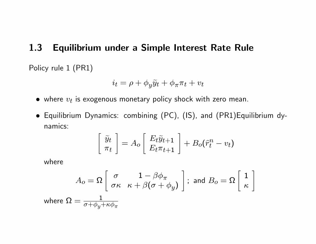
1.3 Equilibrium under a Simple Interest Rate Rule

Policy rule 1 (PR1)

it = �+ �y eyt + ���t + vt

� where vt is exogenous monetary policy shock with zero mean.

� Equilibrium Dynamics: combining (PC), (IS), and (PR1)Equilibrium dy-namics: " eyt

�t

#= Ao

"Eteyt+1Et�t+1

#+Bo(brnt � vt)

where

Ao =

"� 1� ����� �+ �(� + �y)

#; and Bo =

"1�

#

where = 1�+�y+���

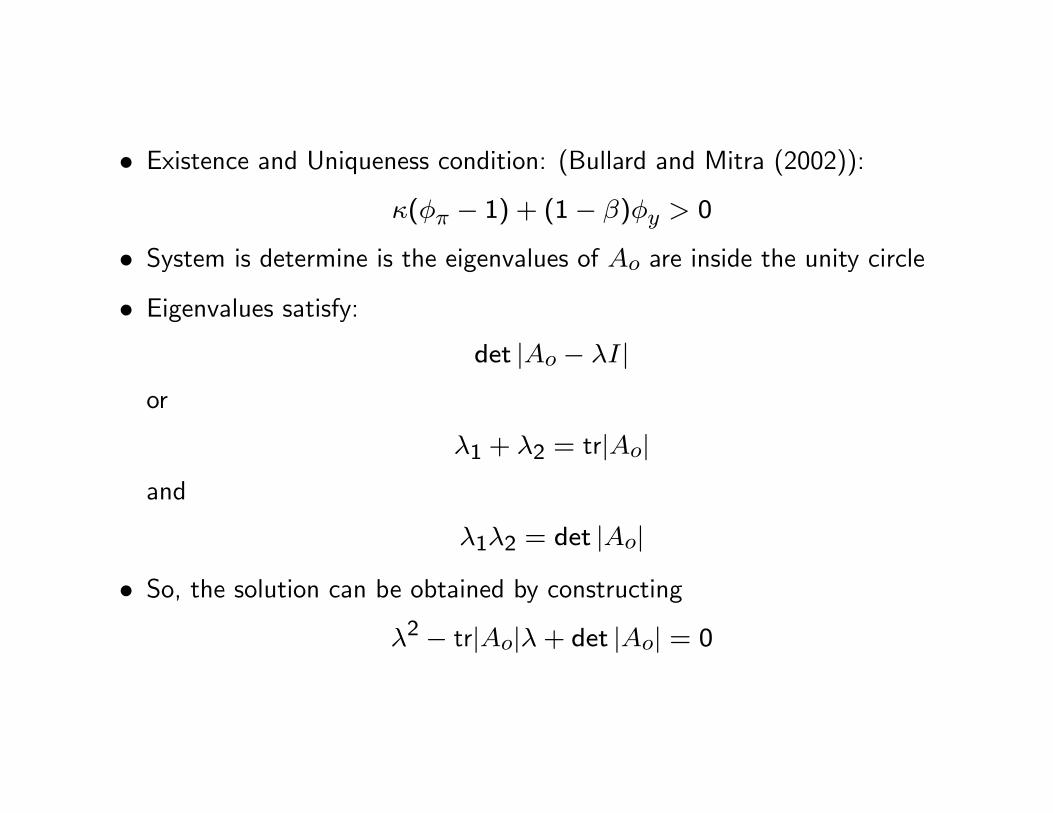
� Existence and Uniqueness condition: (Bullard and Mitra (2002)):

�(�� � 1) + (1� �)�y > 0

� System is determine is the eigenvalues of Ao are inside the unity circle

� Eigenvalues satisfy:det jAo � �Ij

or

�1 + �2 = trjAojand

�1�2 = det jAoj

� So, the solution can be obtained by constructing

�2 � trjAoj�+ det jAoj = 0

� Moreover, if the characteristic polynomials satisfy �2 + a1� + a0 = 0,then the eigenvalue are inside the unit circle if

ja0j < 1

and

ja1j < 1 + a0

� So in this case, the conditions are

j det jAojj < 1

and

j � trjAojj < 1 + det jAoj

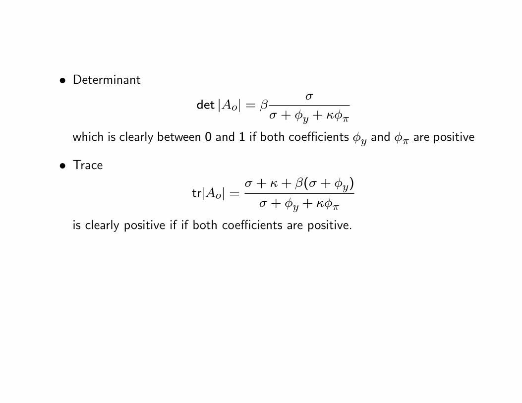
� Determinant

det jAoj = ��

� + �y + ���

which is clearly between 0 and 1 if both coe¢ cients �y and �� are positive

� Trace

trjAoj =� + �+ �(� + �y)

� + �y + ���

is clearly positive if if both coe¢ cients are positive.

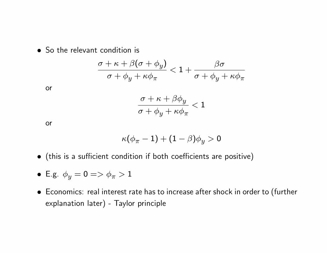
� So the relevant condition is� + �+ �(� + �y)

� + �y + ���< 1 +

��

� + �y + ���or

� + �+ ��y

� + �y + ���< 1

or

�(�� � 1) + (1� �)�y > 0

� (this is a su¢ cient condition if both coe¢ cients are positive)

� E.g. �y = 0 => �� > 1

� Economics: real interest rate has to increase after shock in order to (furtherexplanation later) - Taylor principle

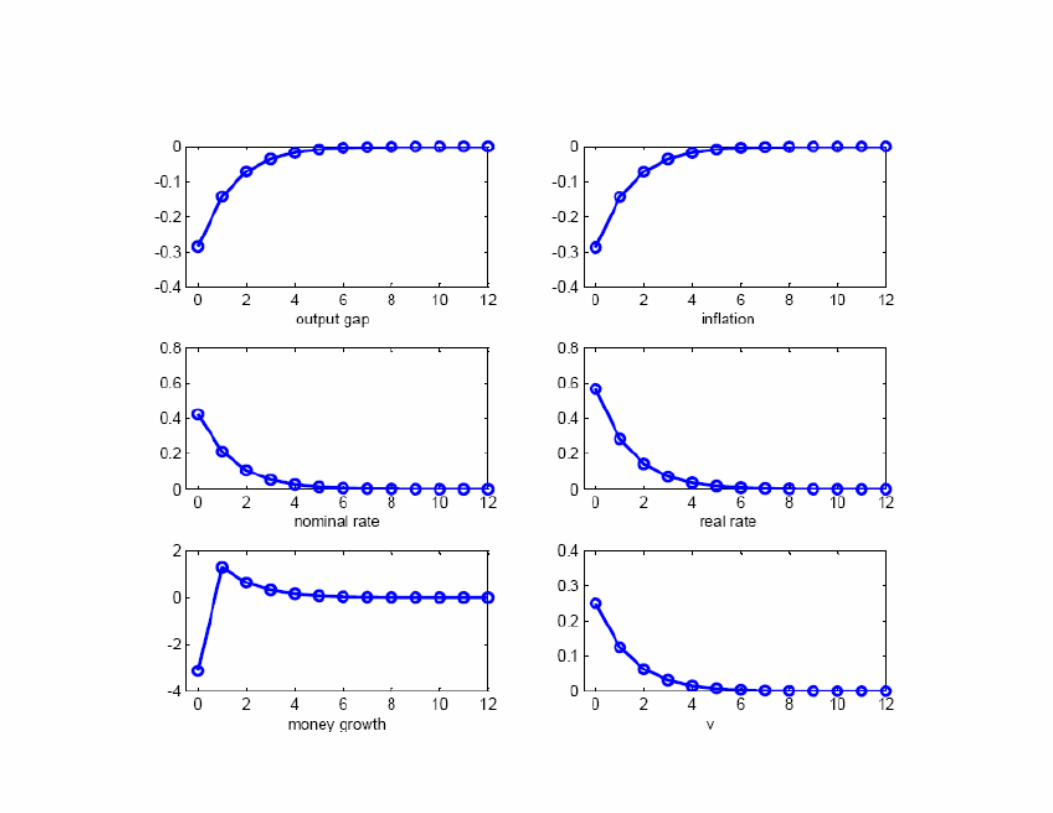
1.4 E¤ect of Monetary Policy shock

Shock process

vt = �vvt�1 + "vt

� if prices were �exible, the increase in nominal rate, which tend to putdownward pressure on demand, would be accompanied by a fall in pricesand an increase expected in�ation, leaving real rates unchanged. As a resultreal activity (and real money balances) would be unchanged (Classicalvertical aggregate supply)

� But given that prices do not adjust, the fall in demand will be accompaniedby a fall in activity (NK upward sloping aggregate supply)

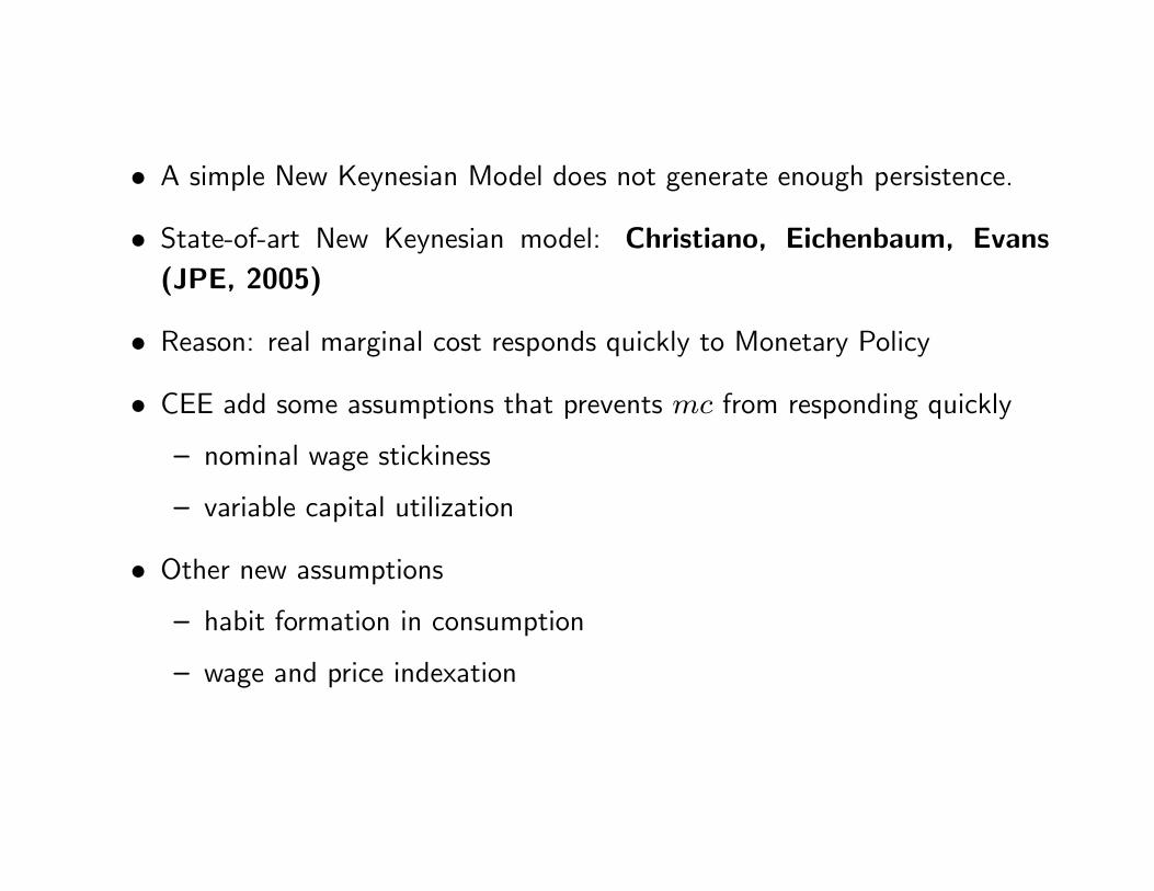
� A simple New Keynesian Model does not generate enough persistence.

� State-of-art New Keynesian model: Christiano, Eichenbaum, Evans(JPE, 2005)

� Reason: real marginal cost responds quickly to Monetary Policy

� CEE add some assumptions that prevents mc from responding quickly

� nominal wage stickiness

� variable capital utilization

� Other new assumptions

� habit formation in consumption

� wage and price indexation

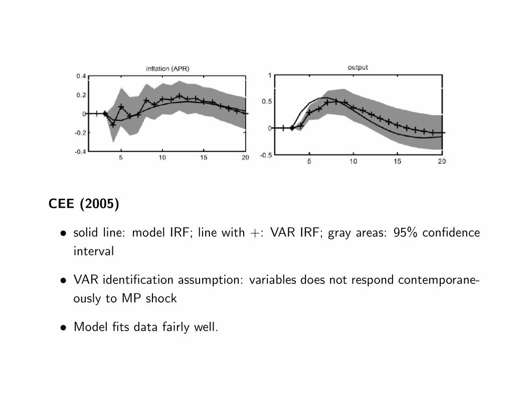
CEE (2005)

� solid line: model IRF; line with +: VAR IRF; gray areas: 95% con�denceinterval

� VAR identi�cation assumption: variables does not respond contemporane-ously to MP shock

� Model �ts data fairly well.

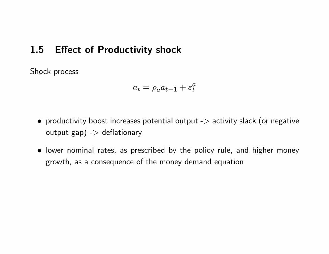
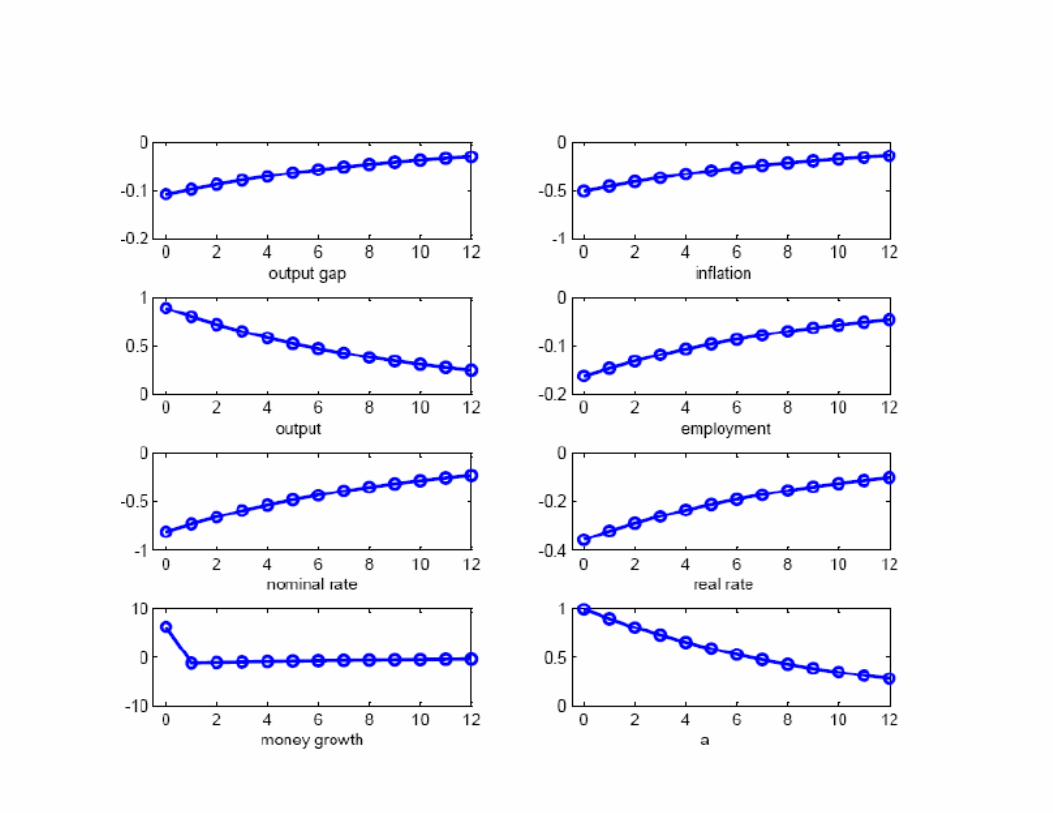
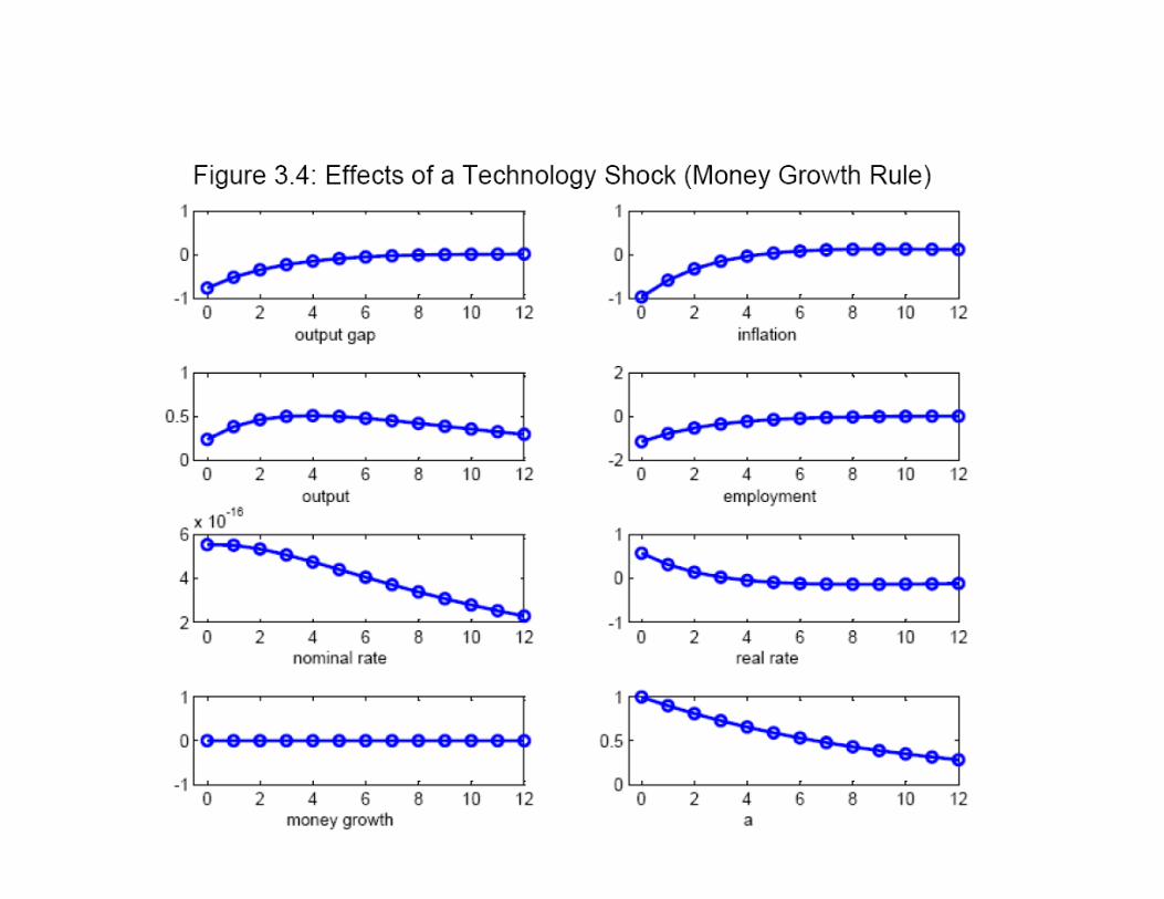
1.5 E¤ect of Productivity shock

Shock process

at = �aat�1 + "at

� productivity boost increases potential output -> activity slack (or negativeoutput gap) -> de�ationary

� lower nominal rates, as prescribed by the policy rule, and higher moneygrowth, as a consequence of the money demand equation

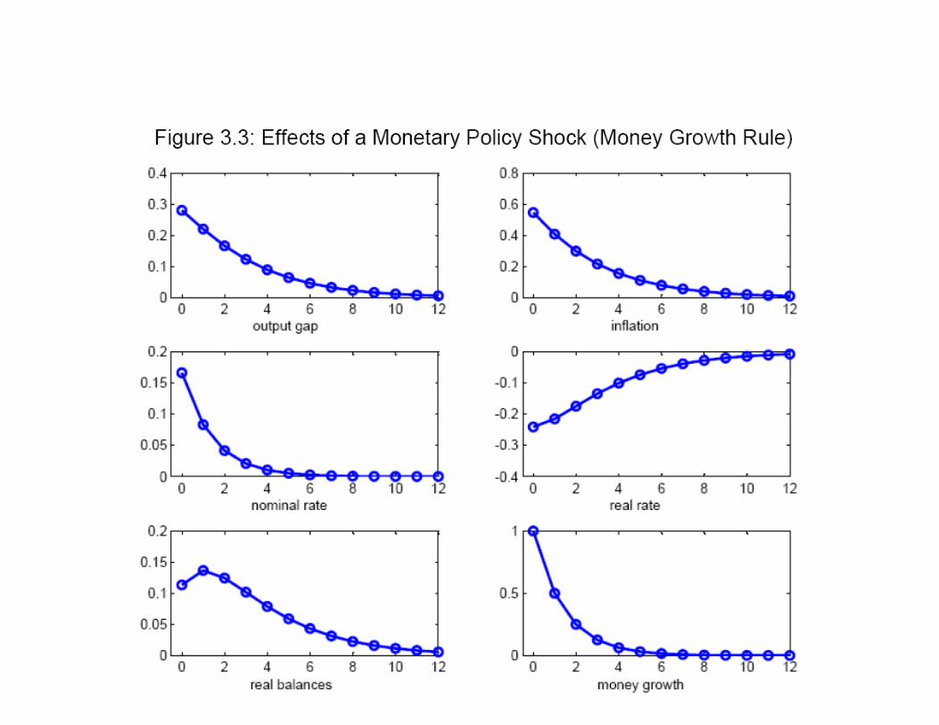
1.6 Equilibrium under an exogenous money growth process

Policy rule 2 (PR2)

�mt = �m�mt�1 + "mt

To simulate the dynamic e¤ects of monetary and productivity shock under theserules you also need to specify a money demand equation

� the e¤ect of a negative "mt shock is similar to an increase in vt

� Productivity shock: under �money rule�nominal interest rate practicallydoes not move so fall in in�ation relative to output is bigger than under�interest rate rule�

1.7 Money-supply vs interest rate rule

� Determinacy of REE:

� REE always determinate under money-supply rule

� REE indeterminate under exogenous interest-rate rule

� REE determinate under � targeting interest-rate rule when ��� > 1 (Taylorprinciple)

� In this sense, money supply is a stronger nominal anchor

� In practice, many Central Banks use interest rates as their policy instru-ments. Why?

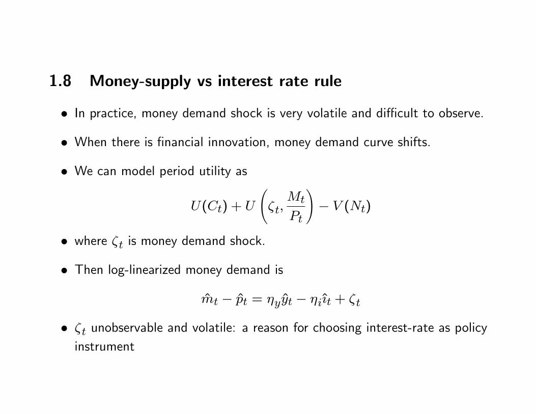
1.8 Money-supply vs interest rate rule

� In practice, money demand shock is very volatile and di¢ cult to observe.

� When there is �nancial innovation, money demand curve shifts.

� We can model period utility as

U(Ct) + U

�t;

Mt

Pt

!� V (Nt)

� where �t is money demand shock.

� Then log-linearized money demand is

mt � pt = �yyt � �i{t + �t

� �t unobservable and volatile: a reason for choosing interest-rate as policyinstrument

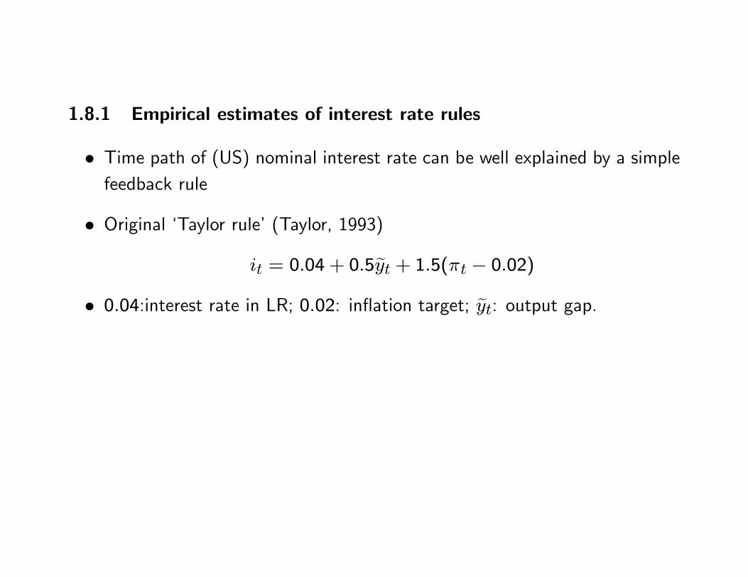
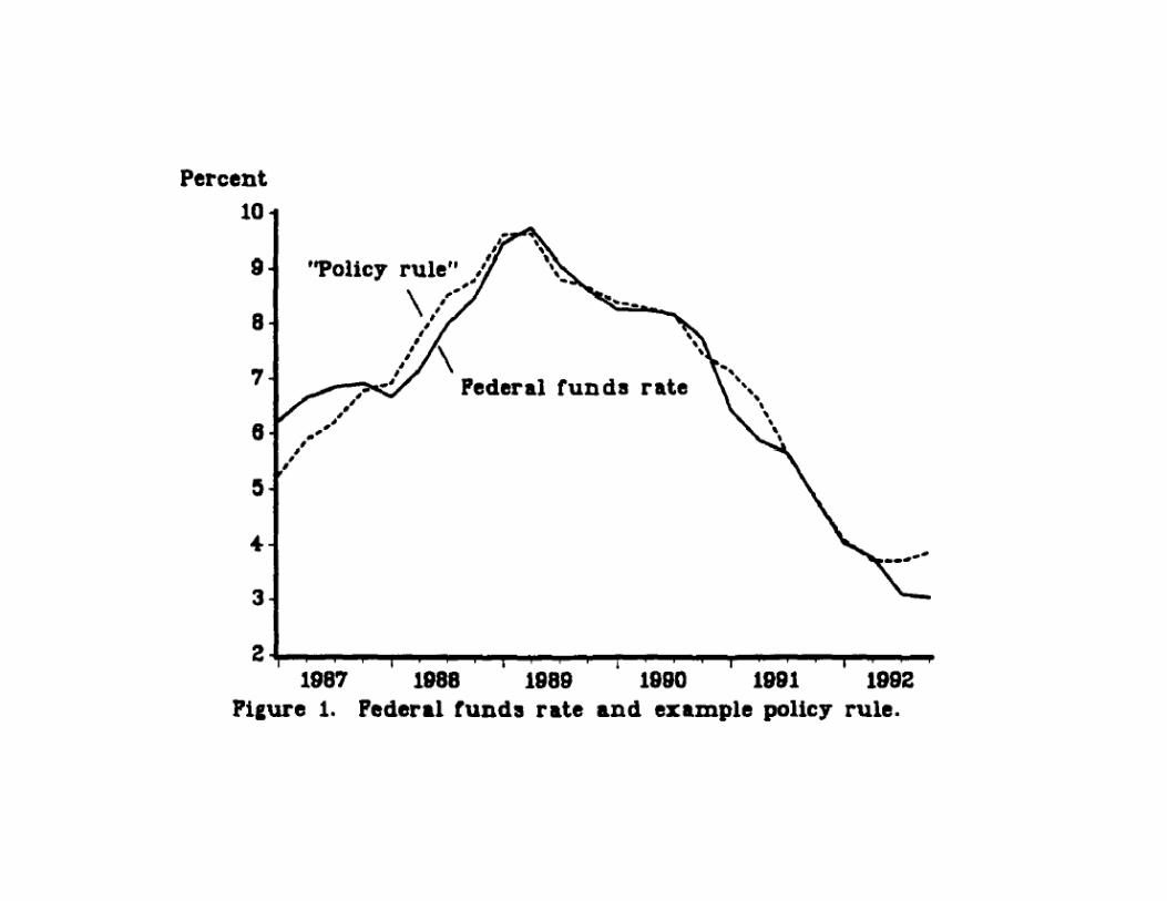
1.8.1 Empirical estimates of interest rate rules

� Time path of (US) nominal interest rate can be well explained by a simplefeedback rule

� Original �Taylor rule�(Taylor, 1993)

it = 0:04 + 0:5eyt + 1:5(�t � 0:02)� 0:04:interest rate in LR; 0:02: in�ation target; eyt: output gap.

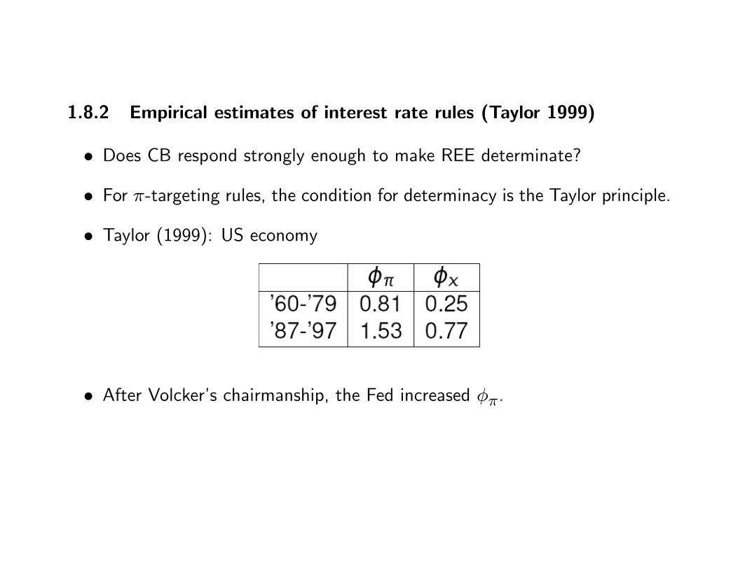
1.8.2 Empirical estimates of interest rate rules (Taylor 1999)

� Does CB respond strongly enough to make REE determinate?

� For �-targeting rules, the condition for determinacy is the Taylor principle.

� Taylor (1999): US economy

� After Volcker�s chairmanship, the Fed increased ��.

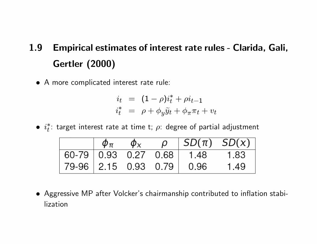
1.9 Empirical estimates of interest rate rules - Clarida, Gali,

Gertler (2000)

� A more complicated interest rate rule:

it = (1� �)i�t + �it�1i�t = �+ �y eyt + ���t + vt

� i�t : target interest rate at time t; �: degree of partial adjustment

� Aggressive MP after Volcker�s chairmanship contributed to in�ation stabi-lization

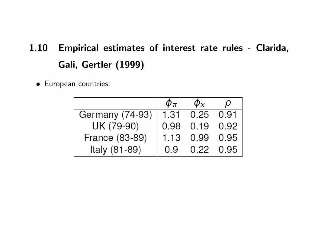
1.10 Empirical estimates of interest rate rules - Clarida,

Gali, Gertler (1999)

� European countries:

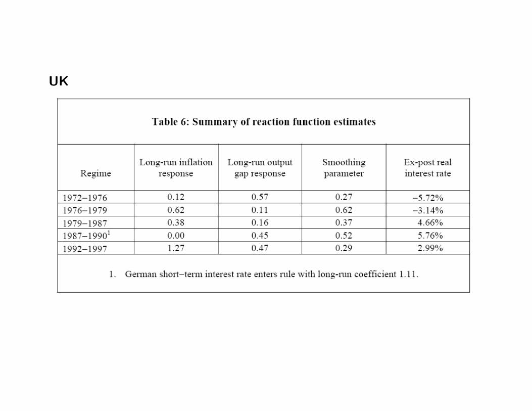
UK

1.11 Policy rules: summary

� Problem of determinacy

� Money supply vs interest rate: money-supply control may be subject touncertainty about money demand shock.

� Empirical studies on interest-rate rules: In the 70s, violation of the Taylorprinciple might have made in�ation volatile

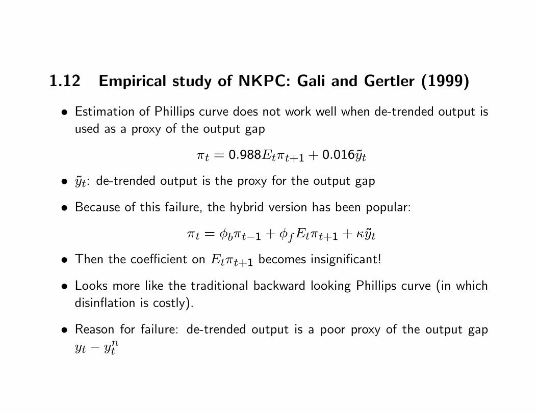
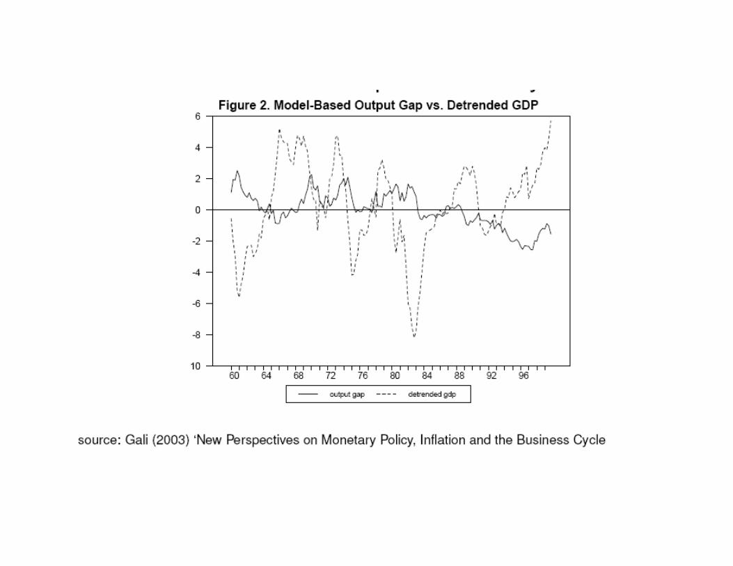
1.12 Empirical study of NKPC: Gali and Gertler (1999)

� Estimation of Phillips curve does not work well when de-trended output isused as a proxy of the output gap

�t = 0:988Et�t+1 + 0:016~yt

� ~yt: de-trended output is the proxy for the output gap

� Because of this failure, the hybrid version has been popular:

�t = �b�t�1 + �fEt�t+1 + �~yt

� Then the coe¢ cient on Et�t+1 becomes insigni�cant!

� Looks more like the traditional backward looking Phillips curve (in whichdisin�ation is costly).

� Reason for failure: de-trended output is a poor proxy of the output gapyt � ynt

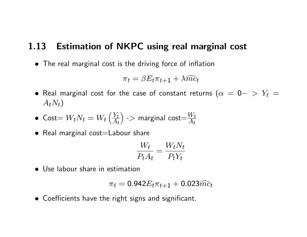
1.13 Estimation of NKPC using real marginal cost

� The real marginal cost is the driving force of in�ation

�t = �Et�t+1 + �dmct� Real marginal cost for the case of constant returns (� = 0� > Yt =

AtNt)

� Cost= WtNt =Wt

�YtAt

�-> marginal cost=Wt

At

� Real marginal cost=Labour shareWt

PtAt=WtNt

PtYt

� Use labour share in estimation

�t = 0:942Et�t+1 + 0:023dmct� Coe¢ cients have the right signs and signi�cant.

Consideration of backward-looking term

� Estimation of the hybrid PC:

�t = �b�t�1 + �fEt�t+1 + �dmct� Estimate of �b = 0:2� 0:3

� Forward �f = 0:6� 0:75

� Forward-looking term more important

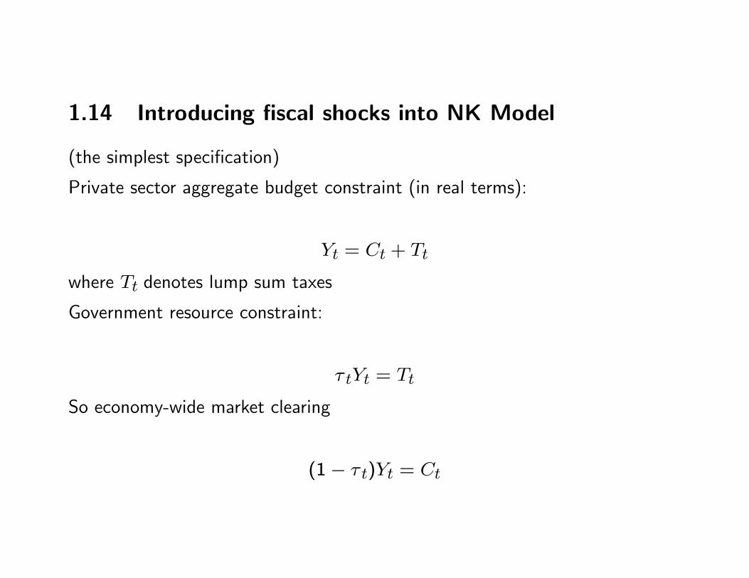
1.14 Introducing �scal shocks into NK Model

(the simplest speci�cation)

Private sector aggregate budget constraint (in real terms):

Yt = Ct + Tt

where Tt denotes lump sum taxes

Government resource constraint:

� tYt = Tt

So economy-wide market clearing

(1� � t)Yt = Ct

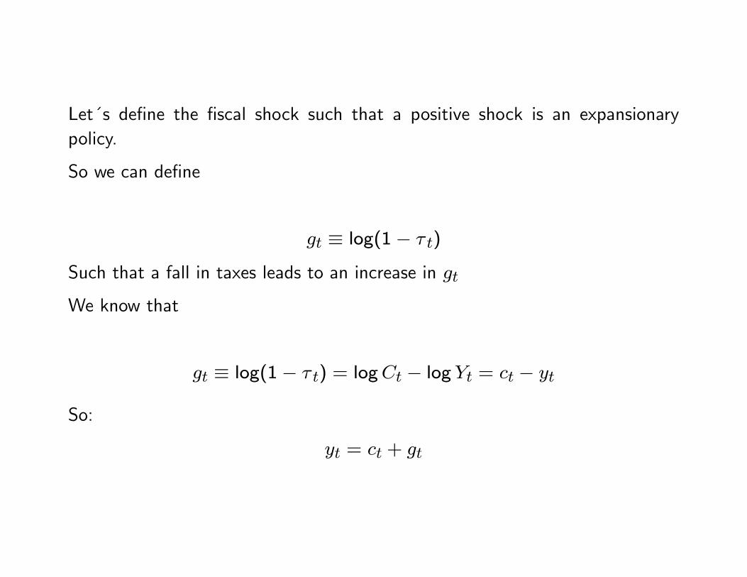
Let´s de�ne the �scal shock such that a positive shock is an expansionarypolicy.

So we can de�ne

gt � log(1� � t)

Such that a fall in taxes leads to an increase in gt

We know that

gt � log(1� � t) = logCt � log Yt = ct � yt

So:

yt = ct + gt

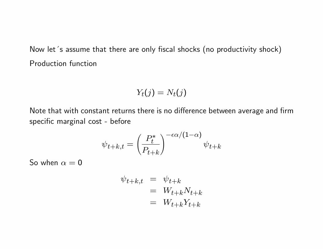
Now let´s assume that there are only �scal shocks (no productivity shock)

Production function

Yt(j) = Nt(j)

Note that with constant returns there is no di¤erence between average and �rmspeci�c marginal cost - before

t+k;t =

P �tPt+k

!���=(1��) t+k

So when � = 0

t+k;t = t+k= Wt+kNt+k= Wt+kYt+k

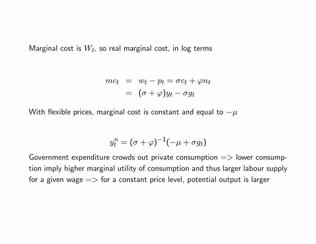
Marginal cost is Wt, so real marginal cost, in log terms

mct = wt � pt = �ct + 'nt

= (� + ')yt � �gt

With �exible prices, marginal cost is constant and equal to ��

ynt = (� + ')�1(��+ �gt)

Government expenditure crowds out private consumption => lower consump-tion imply higher marginal utility of consumption and thus larger labour supplyfor a given wage => for a constant price level, potential output is larger

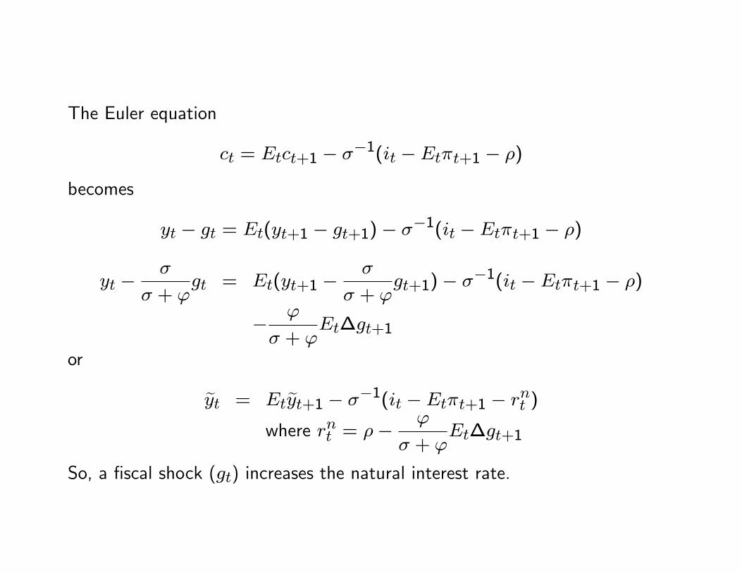
The Euler equation

ct = Etct+1 � ��1(it � Et�t+1 � �)

becomes

yt � gt = Et(yt+1 � gt+1)� ��1(it � Et�t+1 � �)

yt ��

� + 'gt = Et(yt+1 �

�

� + 'gt+1)� ��1(it � Et�t+1 � �)

� '

� + 'Et�gt+1

or

eyt = Eteyt+1 � ��1(it � Et�t+1 � rnt )

where rnt = �� '

� + 'Et�gt+1

So, a �scal shock (gt) increases the natural interest rate.

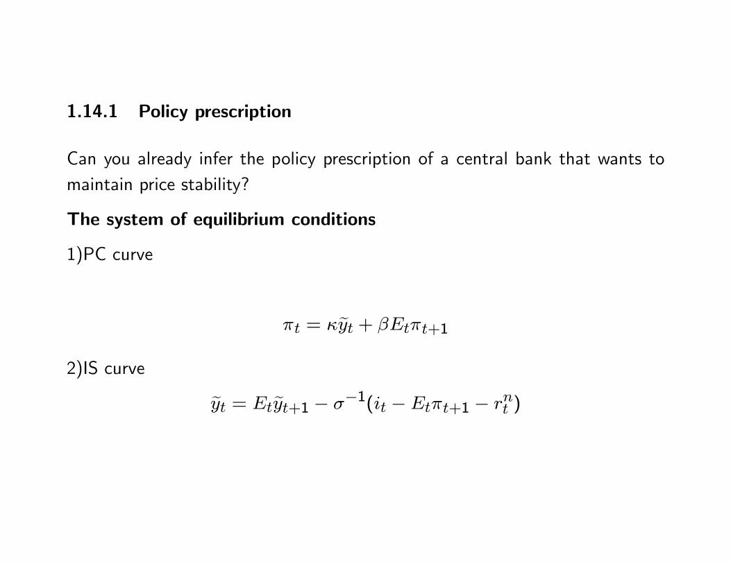
1.14.1 Policy prescription

Can you already infer the policy prescription of a central bank that wants tomaintain price stability?

The system of equilibrium conditions

1)PC curve

�t = �eyt + �Et�t+1

2)IS curve

eyt = Eteyt+1 � ��1(it � Et�t+1 � rnt )

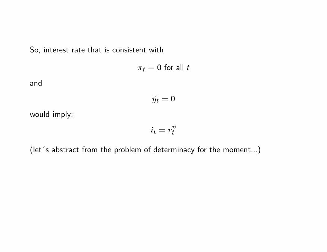
So, interest rate that is consistent with

�t = 0 for all t

and

eyt = 0would imply:

it = rnt

(let´s abstract from the problem of determinacy for the moment...)

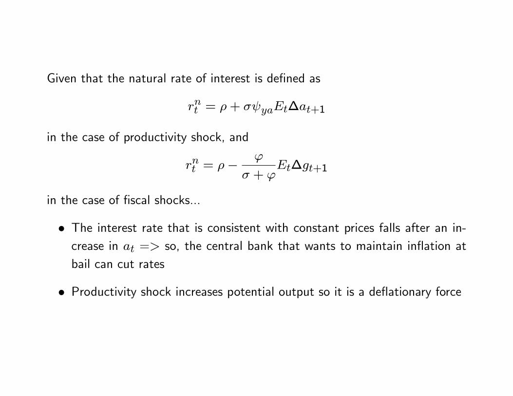
Given that the natural rate of interest is de�ned as

rnt = �+ � yaEt�at+1

in the case of productivity shock, and

rnt = �� '

� + 'Et�gt+1

in the case of �scal shocks...

� The interest rate that is consistent with constant prices falls after an in-crease in at => so, the central bank that wants to maintain in�ation atbail can cut rates

� Productivity shock increases potential output so it is a de�ationary force

� The interest rate that is consistent with constant prices increases after anincrease in gt. => so, the central bank that wants to maintain in�ationat bail have to increase rates

� Two e¤ects of gt� - the shock increases potential output and thus reduces in�ationarypressures for any given level of production.

� - the shock increases aggregate demand and create in�ationary pres-sures

� The second e¤ect dominates - �scal shock normally modelled as demandshock.