Combinatorial Randomized Kaczmarz:An Algebraic Perspective

Sivan Toledo‡

in collaboration withHaim Avron†

Haim Kaplan‡

‡Tel-Aviv University †IBM TJ Watson Research Center

Perspectives on a Randomized Graph Algorithmfor Linear Equations

Sivan Toledo‡

in collaboration withHaim Avron†

Haim Kaplan‡

‡Tel-Aviv University †IBM TJ Watson Research Center

My gift to theSimons Institute for the Theory of Computingis this insight:

In theory,Practitioners can take theoretical results and turn them intofantastic software.

My gift to theSimons Institute for the Theory of Computingis this insight:

In theory,Practitioners can take theoretical results and turn them intofantastic software.

My gift to theSimons Institute for the Theory of Computingis this insight:

In theory,Practitioners can take theoretical results and turn them intofantastic software.In practice, this is often impossible or hard.

Problem Setup

Solve Ax = b with A symmetric, sparse, large, semidefinite

Problem Setup (More Structure)

Solve Ax = b with A symmetric, sparse, large, semidefiniteand diagonally dominant

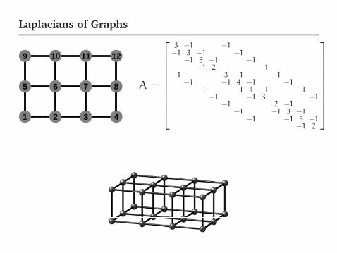
Laplacians of Graphs

1 2 3 4

5 6 7 8

9 10 11 12

A =

⎡⎢⎢⎢⎢⎢⎢⎢⎣

3 −1 −1−1 3 −1 −1

−1 3 −1 −1−1 2 −1

−1 3 −1 −1−1 −1 4 −1 −1

−1 −1 4 −1 −1−1 −1 3 −1

−1 2 −1−1 −1 3 −1

−1 −1 3 −1−1 2

⎤⎥⎥⎥⎥⎥⎥⎥⎦

Ancient History: Direct Solvers, Dense and Sparse,(Preconditioned) Conjugate Gradients

Direct Solvers do not Scale Well

Gauss (Cholesky): factor A = LLT , L triangular, O(n3)arithmetic

Sparse solvers: factor A = PLLTPT , P permutation

• O(n1.5) for 2D meshes,• O(n2) for 3D meshes,• in general depends on size of

approximately-balanced vertex separators

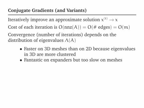
Conjugate Gradients (and Variants)

Iteratively improve an approximate solution x(t) → x

Cost of each iteration is O(nnz(A)) = O(# edges) = O(m)

Convergence (number of iterations) depends on thedistribution of eigenvalues Λ(A)

• Faster on 3D meshes than on 2D because eigenvaluesin 3D are more clustered

• Fantastic on expanders but too slow on meshes

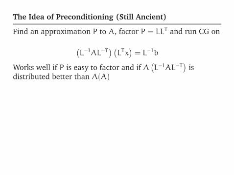
The Idea of Preconditioning (Still Ancient)

Find an approximation P to A, factor P = LLT and run CG on

(L−1AL−T

) (LTx

)= L−1b

Works well if P is easy to factor and if Λ(L−1AL−T

)is

distributed better than Λ(A)

1991-2001: Combinatorial Preconditioners for CG

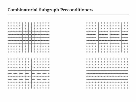
Combinatorial Subgraph Preconditioners

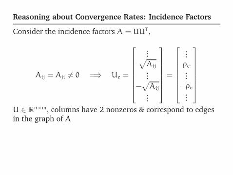
Reasoning about Convergence Rates: Incidence Factors

Consider the incidence factors A = UUT ,

Aij = Aji �= 0 =⇒ Ue =

⎡⎢⎢⎢⎢⎢⎢⎣

...√Aij

...−√

Aij

...

⎤⎥⎥⎥⎥⎥⎥⎦=

⎡⎢⎢⎢⎢⎢⎢⎣

...ρe

...−ρe

...

⎤⎥⎥⎥⎥⎥⎥⎦

U ∈ Rn×m, columns have 2 nonzeros & correspond to edges

in the graph of A

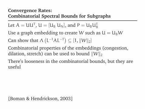
Convergence Rates:Combinatorial Spectral Bounds for Subgraphs

Let A = UUT , U = [UB UN], and P = UBUTB

Use a graph embedding to create W such as U = UBW

Can show that Λ(L−1AL−T

) ⊆ [1, ‖W‖2]Combinatorial properties of the embeddings (congestion,dilation, stretch) can be used to bound ‖W‖2There’s looseness in the combinatorial bounds, but they areuseful

[Boman & Hendrickson, 2003]

Constructing the Subgraph

1991: A maximum spanning tree (MST); Augmented MST[Vaidya]

1997: Explicit construction for regular meshes [Joshi]

2001: Low-stretch trees (can’t easily augment) [Boman &Hendrickson]

2004+: Super-complicated constructions [Spielman & Teng]

2010+: Simpler but not in this talk [Koutis, Miller, & Peng]

Lots of side shows (Toledo & others)

2013: Low-Stretch Trees without Conjugate Gradients

Kelner, Orecchia, Sidford, Zhu (STOC 2013)

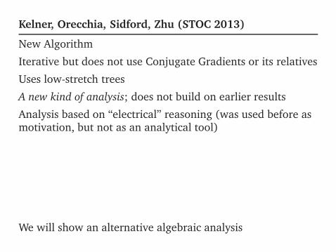
Kelner, Orecchia, Sidford, Zhu (STOC 2013)

New Algorithm

Iterative but does not use Conjugate Gradients or its relatives

Uses low-stretch trees

A new kind of analysis; does not build on earlier results

Analysis based on “electrical” reasoning (was used before asmotivation, but not as an analytical tool)

We will show an alternative algebraic analysis

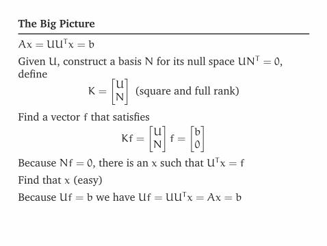
The Big Picture

Ax = UUTx = b

Given U, construct a basis N for its null space UNT = 0,define

K =

[UN

](square and full rank)

Find a vector f that satisfies

Kf =

[UN

]f =

[b0

]

Because Nf = 0, there is an x such that UTx = f

Find that x (easy)

Because Uf = b we have Uf = UUTx = Ax = b

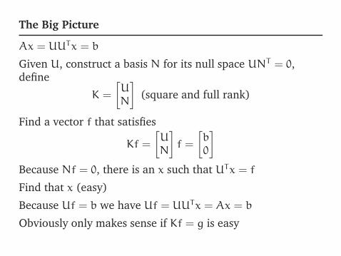
The Big Picture

Ax = UUTx = b

Given U, construct a basis N for its null space UNT = 0,define

K =

[UN

](square and full rank)

Find a vector f that satisfies

Kf =

[UN

]f =

[b0

]

Because Nf = 0, there is an x such that UTx = f

Find that x (easy)

Because Uf = b we have Uf = UUTx = Ax = b

Obviously only makes sense if Kf = g is easy

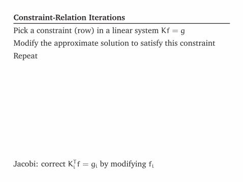
Constraint-Relation Iterations

Pick a constraint (row) in a linear system Kf = g

Modify the approximate solution to satisfy this constraint

Repeat

Jacobi: correct KTi f = gi by modifying fi

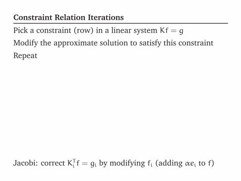
Constraint Relation Iterations

Pick a constraint (row) in a linear system Kf = g

Modify the approximate solution to satisfy this constraint

Repeat

Jacobi: correct KTi f = gi by modifying fi (adding αei to f)

Constraint Relation Iterations

Pick a constraint (row) in a linear system Kf = g

Modify the approximate solution to satisfy this constraint

Repeat

Kaczmarz: correct by adding αKi to f (projection)

Jacobi: correct KTi f = gi by modifying fi (adding αei to f)

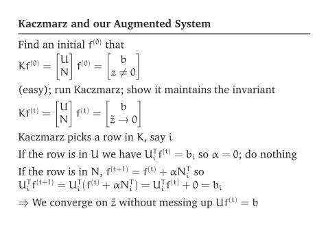
Kaczmarz and our Augmented System

Find an initial f(0) that

Kf(0) =

[UN

]f(0) =

[b

z �= 0

]

(easy); run Kaczmarz; show it maintains the invariant

Kf(t) =

[UN

]f(t) =

[b

z → 0

]

Kaczmarz picks a row in K, say i

If the row is in U we have UTi f

(t) = bi so α = 0; do nothing

If the row is in N, f(t+1) = f(t) + αNTi so

UTi f

(t+1) = UTi (f

(t) + αNTi ) = UT

i f(t) + 0 = bi

⇒ We converge on z without messing up Uf(t) = b

Three Hard Interrelated Challenges

1. How to construct N?

2. How many Kaczmarz iterations will the algorithm do?

3. Running Kaczmarz iterations super efficiently

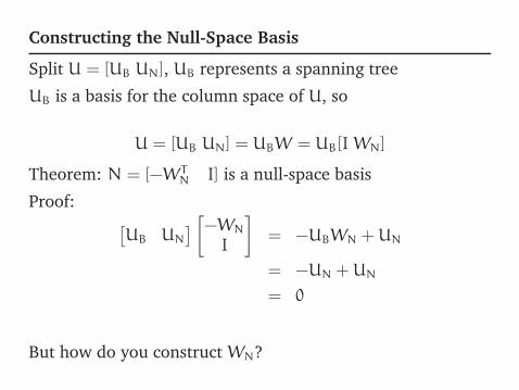
Constructing the Null-Space Basis

Split U = [UB UN], UB represents a spanning tree

UB is a basis for the column space of U, so

U = [UB UN] = UBW = UB[I WN]

Theorem: N = [−WTN I] is a null-space basis

Proof: [UB UN

] [−WN

I

]= −UBWN +UN

= −UN +UN

= 0

But how do you construct WN?

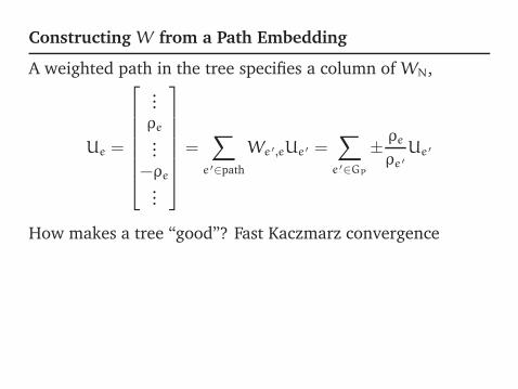
Constructing W from a Path Embedding

A weighted path in the tree specifies a column of WN,

Ue =

⎡⎢⎢⎢⎢⎢⎢⎣

...ρe

...−ρe

...

⎤⎥⎥⎥⎥⎥⎥⎦=

∑e ′∈path

We ′,eUe ′ =∑e ′∈GP

± ρe

ρe ′Ue ′

How makes a tree “good”? Fast Kaczmarz convergence

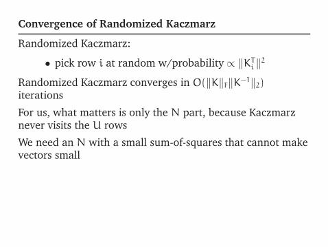
Convergence of Randomized Kaczmarz

Randomized Kaczmarz:

• pick row i at random w/probability ∝ ‖KTi ‖2

Randomized Kaczmarz converges in O(‖K‖F‖K−1‖2)iterations

For us, what matters is only the N part, because Kaczmarznever visits the U rows

We need an N with a small sum-of-squares that cannot makevectors small

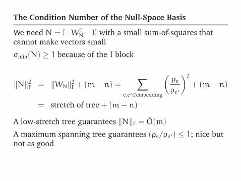
The Condition Number of the Null-Space Basis

We need N = [−WTN I] with a small sum-of-squares that

cannot make vectors small

σmin(N) ≥ 1 because of the I block

‖N‖2F = ‖WN‖2F + (m− n) =∑

e,e ′∈embedding

(ρe

ρe ′

)2

+ (m− n)

= stretch of tree + (m − n)

A low-stretch tree guarantees ‖N‖F = O(m)

A maximum spanning tree guarantees (ρe/ρe ′) ≤ 1; nice butnot as good

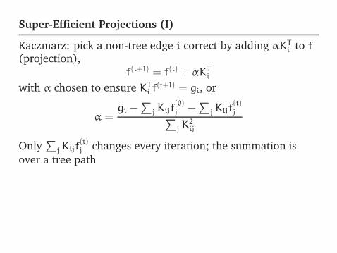
Super-Efficient Projections (I)

Kaczmarz: pick a non-tree edge i correct by adding αKTi to f

(projection),f(t+1) = f(t) + αKT

i

with α chosen to ensure KTi f

(t+1) = gi, or

α =gi −

∑j Kijf

(0)j −

∑j Kijf

(t)j∑

j K2ij

Only∑

j Kijf(t)j changes every iteration; the summation is

over a tree path

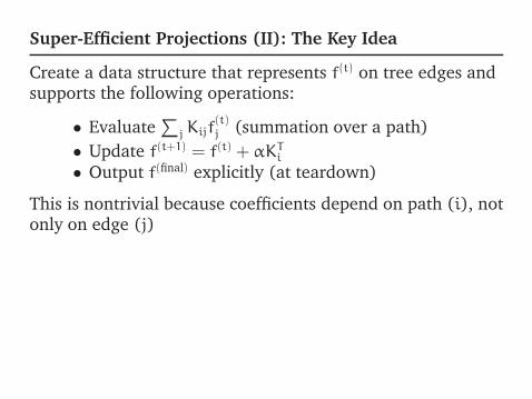
Super-Efficient Projections (II): The Key Idea

Create a data structure that represents f(t) on tree edges andsupports the following operations:

• Evaluate∑

j Kijf(t)j (summation over a path)

• Update f(t+1) = f(t) + αKTi

• Output f(final) explicitly (at teardown)

This is nontrivial because coefficients depend on path (i), notonly on edge (j)

Super-Efficient Projections (III): The Data Structure

An algebraic transformation allows us to remove pathdependency:

• Evaluate∑

j βjf(t)j (summation over a path)

• Update f(t+1) = f(t) + αKTi

• Output f(final) explicitly (at teardown)

O(logn) per operation using a hierarchical data structurederived from Sleator and Tarjan’s dynamic trees

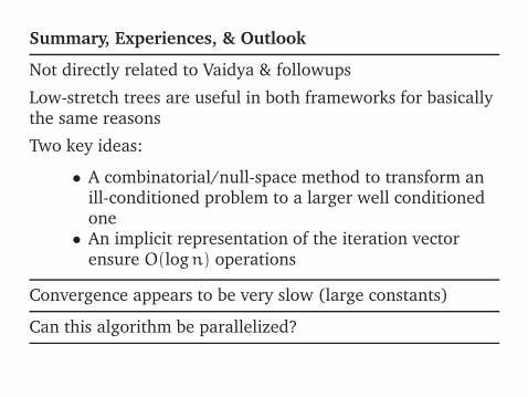
Summary, Experiences, & Outlook

Not directly related to Vaidya & followups

Low-stretch trees are useful in both frameworks for basicallythe same reasons

Two key ideas:

• A combinatorial/null-space method to transform anill-conditioned problem to a larger well conditionedone

• An implicit representation of the iteration vectorensure O(logn) operations

Convergence appears to be very slow (large constants)

Can this algorithm be parallelized?