1

Slot Machine Stopping Decisions: Evidence for Prospect Theory Preferences?

Jaimie W. Lien

1

Tsinghua University

School of Economics and Management

Version: August 29th

, 2011

Abstract

This paper uses a novel dataset from slot machines at a casino to provide a new empirical test

for Prospect Theory risk preferences in the field. My findings are threefold: 1. Unconditional on stakes

level, casino patrons prefer to stop gambling when they are near the break-even point of zero net

winnings; 2. Conditional on the stakes level, casino patrons tend to stop gambling bunched near a

stakes-specific reference point; 3. Conditional on the stakes level, casino patrons prefer to stop

gambling when they are above the reference point than when they are below it. These results are

difficult to reconcile with a standard Expected Utility model, but are entirely consistent with the value

function shape proposed by Prospect Theory. My empirical methodology makes use of the independent

and identical nature of slot machine payout distributions (legally enforced), and the approximate risk-

neutrality predicted by Expected Utility Theory over small stakes gambles, to statistically reject the

hypothesis that casino patrons‟ quitting decisions were independent of their winnings earned that day.

A contribution of the methodology is that it permits a test of the reference-dependence implied by

Prospect Theory, without requiring a theoretical specification or estimation of the reference point.

Keywords: Uncertainty, Prospect Theory, Expected Utility

JEL: D03, D12, D81

1 jwlien@sem.tsinghua.edu.cn. I am grateful to my dissertation advisors Vincent Crawford and Julie Cullen for their

encouragement and guidance, and an anonymous casino which generously allowed me to use their data for this study. For

helpful comments and conversations, I also thank Kristy Buzard, Gray Calhoun, Rachel Croson, Gordon Dahl, David Eil,

Graham Elliott, Uri Gneezy, Chulyoung Kim, Craig McIntosh, Juanjuan Meng, Jason Shachat, Uri Simonsohn, Joel Sobel,

and participants in the UCSD Micro theory lunch seminar. All errors are my own.

2

1. Introduction2

Do slot machine gamblers behave consistently with the Prospect Theory value function? This

paper presents new evidence on whether risky decisions can be most adequately accounted for with a

neoclassical model of choice under uncertainty or a reference-dependent model, using field data from a

unique dataset of slot machine gamblers. While previous studies have tested for forms of reference

dependence in the field, this study presents new evidence of irregularities relative to the standard

neoclassical model from a previously untested field setting.

I analyze data gathered over the course of one month at a North American casino using magnetic

strip cards, which track nearly 2400 gamblers‟ activity for a single visit, recording each gambler‟s

numbers of bets placed, wagers, and winnings. The data provide clear statistical evidence of reference

dependence in winnings for slot machine gamblers that is consistent with the value function proposed by

Prospect Theory (PT; Kahneman and Tversky 1979), rejecting implications of Expected Utility (EU)

under the utility of gambling framework proposed by Conlisk (1993). A further contribution is that the

empirical methodology used in this paper to test for reference-dependence does not require specifying the

reference point, but rather allows it to appear naturally in the data via realized payoff distributions, as a

function of the observed wager sizes the gamblers took.

The workhorse neoclassical model EU, assumes that a person maximizes the mathematical

expectation of his or her von Neumann-Morgenstern utility function defined over wealth levels. PT is the

workhorse behavioral model, which assumes that an individual‟s decisions under uncertainty are

determined by preferences over distributions of total final winnings relative to a reference point such as

the status quo ante or expected return – a feature known as reference-dependence. In addition, PT value

depends on whether the level of winnings is a gain or loss relative to this reference point, with losses of a

given magnitude lowering value by more than gains of the same magnitude raise it – the key feature of PT

known as loss aversion.3

I assume that a gambler‟s decision to stop making bets is determined by two main factors: realized

winnings as the PT or EU theories suggest, and an intrinsic utility of gambling derived from the

anticipation of the bet‟s outcome as proposed by Conlisk (1993). The utility of gambling component is

likely to decrease marginally in the long run as a result of gambling fatigue. My analysis assumes that the

utility derived purely from pulling the slot machine lever is independent of the outcome of each pull and

may be heterogeneous across gamblers.4 So each gambler has their own pace at which playing slot

machines becomes tiresome, but all gamblers are assumed to have approximately similar preferences over

the wealth resulting from the gambles – in the case of EU, a slightly positive marginal utility of winnings

so that winning is preferred to losing, but risk aversion over small stakes is minimal – and in the case of

PT, a similar preference for winning over losing except that risk aversion is markedly higher near a

particular outcome which gamblers consider the reference point. While the data do not have the capability

of ruling out all variations of neoclassical models, they distinctly show a higher propensity to quit

gambling at a reference point, and under a utility of gambling assumption of the form suggested by

Conlisk (1993), support the break-even effect of Thaler and Johnson (1990) being greater than the house

money effect.

The slot machine environment is a simple and relatively controlled setting to test for EU and PT in

the field. The environment is constant since machines pay out with the same probabilities regardless of

2 A list of acronyms and variables used throughout the paper and their meanings is provided in Appendix A.

3 Kahneman and Tversky‟s original Prospect Theory formulation also allowed for non-linear probability weighting, which this

field data is not rich enough to test. Accounting for non-standard beliefs may be more properly addressed with a future

experiment. 4 This rules out wealth-dependent utility of gambling, such as valuing the intrinsic act of gambling to a greater degree while

winning or losing.

3

day of the week or time of day. Furthermore, the outcomes of individual bets are random and independent

of previous bets by legal regulation, and there is no particular skill required by the decision-maker.5

Due to data limitations which do not allow observation of every single bet made, I consider only a

gambler‟s total number of bets over all machines played and his or her total net winnings for the visit.

Following the main analysis of Post, van den Assem, Baltussen, and Thaler (2008), I ignore the option

value of continuing to make bets, assuming that gamblers make the decision whether to quit or continue

myopically, one bet at a time, given that they have already decided to visit the casino (due to enjoyment

of gambling, and other potential factors which may have led him there).6

Making use of the fact that individual bet outcomes are serially independent, the central limit

theorem predicts that regardless of the original distribution of returns for a single bet, for a sufficiently

large number of bets taken, an individual gambler‟s sum of winnings up until that point should be

distributed normally.7 Therefore in the cross-section of individuals, if we assume that individuals quit

approximately randomly (and independently of one another) as suggested by EU, then the empirical

distribution of winning levels observed in the data for gamblers who took the same number and type of

bets should also be normally distributed.

By extending this basic reasoning to allow for aggregation over bets and wager sizes, and

supplementing with simulations for comparison purposes, the analysis shows that the distribution of

actual realized winnings has substantially higher kurtosis (4th

moment) than a normal distribution, or

simulations accounting for gambler heterogeneity. Since excess kurtosis means a higher peaked

probability distribution, this is an indication of the presence of the key feature of PT, loss aversion with

respect to the reference point where individuals quitting decisions are disproportionally concentrated. This

result confirms the predictions of PT in a dynamic setting, replicating Thaler and Johnson‟s (1990) break-

even effect which predicts lower likelihood of quitting while losing relative to the reference point, and the

house money effect which predicts the similar result for winning relative to the reference point.

In addition, the empirical distribution of winnings are more positively skewed than simulations

suggest, meaning that gamblers were more likely to quit while being “ahead” (relative to the reference

point) instead of quitting while “behind.” This is consistent with the hypothesis that the PT value function

has the additional feature of diminishing sensitivity in the gains and loss segments, making winning

individuals risk-averse and losing individuals risk-loving. So, while on the margin individuals are still

most likely to quit near the reference point, they are even less likely to quit while behind compared to

while ahead.

The rest of the paper is organized as follows. Section 2 provides a brief review of related literature.

Section 3 describes the key features of EU and PT models of decision making under uncertainty and

derives their implications for gambling behavior. Readers already familiar with EU, PT, and related

empirical literature might skip to Section 3.3. Section 4 describes the data. Section 5 discusses the

assumptions and empirical strategy. Section 6 reports the results. Section 7 discusses possible future work

and concludes.

2. Literature review

5 See Zangeneh, Blaszczynski, and Turner (2007), Chapter 2.

6 See Barberis (2009) for a theoretical analysis of both the decision to visit the casino, as well as the gambler‟s behavior once

inside the casino using a non-naïve PT framework. 7 Appendix D discusses the speed of convergence of cumulative winnings to a normal distribution under the assumption that

the underlying payout distribution is exponential. While it is difficult to find information about the true payout of slot machine

distributions, the exponential distribution is a reasonable approximation due to the fact that it implies paying out low or

negative amounts with the highest probability (ie. The gambler loses most of the time), and increasing amounts with lower and

lower probability (ie. The likelihood of a huge jackpot is small). Under this assumption, a distribution that is not substantially

different from normal is obtained after fairly few total bets taken.

4

Camerer (1998) surveys a number of field studies which have used PT to explain puzzles that are

hard to reconcile in an EU framework. For example, Benartzi and Thaler (1997) proposed a PT

explanation of the equity premium puzzle – the phenomenon of risk premiums on equity returns being

systematically much higher than a reasonable risk-averse EU investor would require in order to hold

equity rather than bonds. They suggested that the premium is so high because it must compensate not only

for investors‟ risk aversion, but also for their loss aversion. Camerer, Babcock, Loewenstein and Thaler

(1997) (see also Koszegi and Rabin (2006)) considered the role of reference dependence and loss aversion

in cabdrivers‟ labor supply decisions, finding that drivers worked fewer hours when average daily wages

were high, and more hours when daily wages were low – a behavior contrary to predictions of classical

intertemporal labor supply substitution, but consistent with loss averse preferences in daily income.

In additional support for loss aversion, Odean (1998) shows that investors, via a “disposition

effect,” tend to sell stocks whose purchase prices allow them to realize a gain, significantly more often

than otherwise equivalent stocks whose sale would yield a loss. He suggests a PT explanation for this

systematically different treatment of gains and losses (also see Barberis and Xiong (2006)). Weber and

Camerer (1998) confirm the disposition effect in the experimental lab. Similar to Odean (1998)‟s field

work on stock market investors, Genesove and Mayer (2001) show that condominium owners seeking to

sell their properties but facing an expected loss in the market, posted asking prices that were

systematically higher than owners of similar condominiums whose expected selling price would yield a

gain.

An early, key experimental study by Thaler and Johnson (1990) extends PT by focusing on the

impact of previous gains and losses on current decision-making under uncertainty, thus applying PT to an

explicitly dynamic setting. Thaler and Johnson find that risk aversion as revealed by choices, tends to

decrease after a previous gain, which they call the “house money effect”. They also find that risk aversion

decreases after a previous loss, provided that a gamble offers the opportunity for a person to break even,

which they call the “break-even effect”.

Perhaps the most direct field evidence in support of Thaler and Johnson‟s dynamic generalization

of PT is Post, van den Assem, Baltussen, and Thaler (2008), who examine decisions of contestants in the

television show “Deal or No Deal?” In the show, contestants go through several rounds of deciding

between risk-free „bank offers‟ and the pursuit of a final prize of unknown value in a suitcase. Post et al

find that as information about the final prize is uncovered in each round of the game, contestants were

more likely to reject generous risk-free offers (often exceeding the expected value of the final prize), after

uncovering information that suggested either a very favorable or unfavorable final prize. In other words,

contestants were less risk-averse when evidence supported the idea that their final prize was either very

bad (“break even effect”) or very good (“house money effect”) relative to reasonable expectations – a

pattern most easily reconciled using PT.

Prospect Theory driven behavior has also been tested in sports settings, using effort as a measure

of distaste for outcomes. Pope and Schweitzer (forthcoming), find evidence for loss aversion in

professional golfers‟ decisions using par as the reference point. Golfers in the PGA Tour are more

accurate in hitting putts when they are at or above par (loss domain), than when they are below par (gains

domain). Similarly, Berger and Pope (2009) find that NCAA and NBA teams that are slightly behind at

halftime win more often than would otherwise be expected.

3. Models of decisions under uncertainty

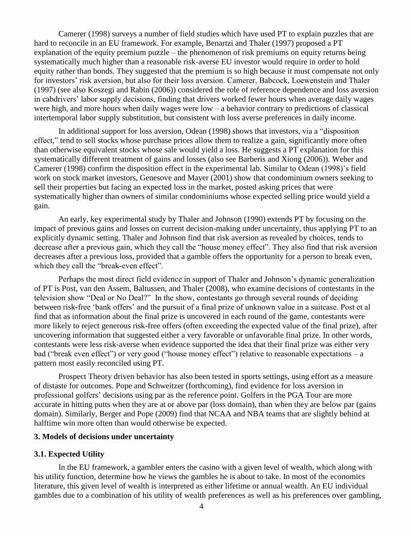
3.1. Expected Utility

In the EU framework, a gambler enters the casino with a given level of wealth, which along with

his utility function, determine how he views the gambles he is about to take. In most of the economics

literature, this given level of wealth is interpreted as either lifetime or annual wealth. An EU individual

gambles due to a combination of his utility of wealth preferences as well as his preferences over gambling,

5

both of which interact to determine at what point he decides to stop. He stops gambling when his utility of

gambling no longer compensates him adequately for the change in Expected Utility of wealth anticipated

from the next bet.

EU normally assumes that utility of wealth is concave, often further assuming that the individual‟s

level of absolute risk aversion decreases as wealth increases - so that increases in wealth, other things

equal, make a person less averse to mean-preserving risks involving absolute changes in wealth. A typical

neoclassical utility function looks like the one in Figure 1 below, which shows a “flexible expo utility

function” (with parameters α = 0.5 and β = 0.5). This family of functions allows the individual‟s risk-

aversion to be flexible in both relative and absolute terms with respect to wealth.8

Attitudes toward risk in the EU framework are completely determined by a gambler‟s wealth level.

For small stakes gambles such as slot machines, where the typical wager is only a fraction of a dollar at a

time, a small amount relative to lifetime or annual income. Under these conditions, a differentiable von

Neumann-Morgenstern (VNM) utility function implies that people are approximately risk neutral. Further,

even for variations in wealth as large as a whole visit‟s winnings or losses at a casino, which are on the

order of less than $1000 for 97% of people in the sample, significant variation in an individual‟s absolute

risk aversion is unlikely. An EU individual with time-separable preferences will value an additional bet

about the same everywhere within the range of wealth variation in a day at the casino, and therefore has

no preference for quitting at one level of casino winnings over another. The EU individual‟s quitting

decision can therefore be approximately interpreted as random with respect to winnings. Figure 1: Example VNM Utility Function

neoclassical utility

0

0.5

1

1.5

2

2.5

0 3 6 9 12 15 18 21 24 27 30 33 36 39 42 45

wealth

utility

In this essay I avoid the scaling concern discussed by Rabin (2000) and Rabin and Thaler (2001)

by confining the analysis to the small to moderate risks casino gamblers encountered in the dataset. 9

8 Flexible Expo utility nests Constant Relative Risk Aversion (CRRA) utility as the special case where α→∞ and Constant

Absolute Risk Aversion (CARA) utility as the special case where β = 0. The original formulation is credited to Saha (1993),

and is utilized in Post et al. (2008) with the formulation u(x) = [1-exp(-α(W+x)1-β

)]/ α, also used in the above figure, where W

is ex-ante wealth, and x is the net outcome of the gamble. 9 Rabin (2000) and Rabin and Thaler (2001) take this argument a step further, arguing that EU cannot simultaneously explain

people‟s attitudes toward small and large risks, because the moderate risk aversion commonly observed over small stakes

gambles implies, in an EU framework, unreasonably high risk aversion over gambles of larger stakes. This is due to the fact

that marginal utility would have to be dropping very steeply from the person‟s current level of wealth in the event of losing the

small stakes gamble in order for them to reject it, which suggests that they will have to reject any gamble which poses a

potentially larger loss. The specific example that Rabin and Thaler give is “Johnny is a risk averse, EU maximizer, who always

turns down a 50-50 gamble of losing $10 or gaining $11. …what is the biggest Y such that we know Johnny will turn down a

50-50 lose $100, gain $Y bet?” The answer is “Johnny will reject the bet no matter what Y is.” The intuitive interpretation is

6

3.2. Prospect Theory

Unlike EU, PT assumes that individuals evaluate the decision on whether or not to take a

particular gamble based on their current position relative to some reference point. To close the model it is

necessary to specify what determines the reference point. This has been done in various ways. For

example the reference point might be determined by a person‟s expectations (Koszegi and Rabin 2007), or

the status quo ante (Thaler and Johnson 1990). Since my econometric tests rely only on rejecting the

normal distribution and not the exact value of the reference point, I do not attempt to estimate it, although

its value can be inferred by examining where in the winnings distribution quitting tends to concentrate.

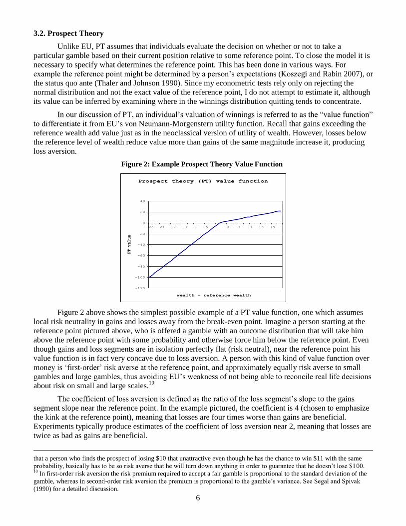
In our discussion of PT, an individual‟s valuation of winnings is referred to as the “value function”

to differentiate it from EU‟s von Neumann-Morgenstern utility function. Recall that gains exceeding the

reference wealth add value just as in the neoclassical version of utility of wealth. However, losses below

the reference level of wealth reduce value more than gains of the same magnitude increase it, producing

loss aversion.

Figure 2: Example Prospect Theory Value Function

Prospect theory (PT) value function

-120

-100

-80

-60

-40

-20

0

20

40

-25 -21 -17 -13 -9 -5 -1 3 7 11 15 19

wealth - reference wealth

PT value

Figure 2 above shows the simplest possible example of a PT value function, one which assumes

local risk neutrality in gains and losses away from the break-even point. Imagine a person starting at the

reference point pictured above, who is offered a gamble with an outcome distribution that will take him

above the reference point with some probability and otherwise force him below the reference point. Even

though gains and loss segments are in isolation perfectly flat (risk neutral), near the reference point his

value function is in fact very concave due to loss aversion. A person with this kind of value function over

money is „first-order‟ risk averse at the reference point, and approximately equally risk averse to small

gambles and large gambles, thus avoiding EU‟s weakness of not being able to reconcile real life decisions

about risk on small and large scales.10

The coefficient of loss aversion is defined as the ratio of the loss segment‟s slope to the gains

segment slope near the reference point. In the example pictured, the coefficient is 4 (chosen to emphasize

the kink at the reference point), meaning that losses are four times worse than gains are beneficial.

Experiments typically produce estimates of the coefficient of loss aversion near 2, meaning that losses are

twice as bad as gains are beneficial.

that a person who finds the prospect of losing $10 that unattractive even though he has the chance to win $11 with the same

probability, basically has to be so risk averse that he will turn down anything in order to guarantee that he doesn‟t lose $100. 10

In first-order risk aversion the risk premium required to accept a fair gamble is proportional to the standard deviation of the

gamble, whereas in second-order risk aversion the premium is proportional to the gamble‟s variance. See Segal and Spivak

(1990) for a detailed discussion.

7

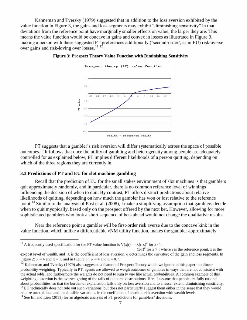
Kahneman and Tversky (1979) suggested that in addition to the loss aversion exhibited by the

value function in Figure 3, the gains and loss segments may exhibit “diminishing sensitivity” in that

deviations from the reference point have marginally smaller effects on value, the larger they are. This

means the value function would be concave in gains and convex in losses as illustrated in Figure 3,

making a person with these suggested PT preferences additionally („second-order‟, as in EU) risk-averse

over gains and risk-loving over losses.11

12

Figure 3: Prospect Theory Value Function with Diminishing Sensitivity

Prospect theory (PT) value function

-50

-40

-30

-20

-10

0

10

20

-25 -21 -17 -13 -9 -5 -1 3 7 11 15 19

wealth - reference wealth

PT value

PT suggests that a gambler‟s risk aversion will differ systematically across the space of possible

outcomes.13

It follows that once the utility of gambling and heterogeneity among people are adequately

controlled for as explained below, PT implies different likelihoods of a person quitting, depending on

which of the three regions they are currently in.

3.3 Predictions of PT and EU for slot machine gambling

Recall that the prediction of EU for the small stakes environment of slot machines is that gamblers

quit approximately randomly, and in particular, there is no common reference level of winnings

influencing the decision of when to quit. By contrast, PT offers distinct predictions about relative

likelihoods of quitting, depending on how much the gambler has won or lost relative to the reference

point.14

Similar to the analysis of Post et al. (2008), I make a simplifying assumption that gamblers decide

when to quit myopically, based only on the prospect offered by the next bet. However, allowing for more

sophisticated gamblers who look a short sequence of bets ahead would not change the qualitative results.

Near the reference point a gambler will be first-order risk averse due to the concave kink in the

value function, which unlike a differentiable vNM utility function, makes the gambler approximately

11

A frequently used specification for the PT value function is V(x|r) = -λ(r-x)α for x ≤ r

(x-r)α for x > r where r is the reference point, x is the

ex-post level of wealth, and λ is the coefficient of loss aversion. α determines the curvature of the gain and loss segments. In

Figure 2: λ = 4 and α = 1, and in Figure 3: λ = 4 and α = 0.7. 12

Kahneman and Tversky (1979) also suggested a feature of Prospect Theory which we ignore in this paper: nonlinear

probability weighting. Typically in PT, agents are allowed to weigh outcomes of gambles in ways that are not consistent with

the actual odds, and furthermore the weights do not need to sum to one like actual probabilities. A common example of this

weighting distortion is the overweighting of the tails of outcome distributions. Here I assume that people are fully rational

about probabilities, so that the burden of explanation falls only on loss aversion and to a lesser extent, diminishing sensitivity. 13

EU technically does not rule out such variations, but does not particularly suggest them either in the sense that they would

require unexplained and implausible variations in the coefficient of absolute risk aversion with wealth levels. 14

See Eil and Lien (2011) for an algebraic analysis of PT predictions for gamblers‟ decisions.

8

equally averse to small and large risks. Therefore at net winnings levels near the reference point, a person

is highly unwilling to take additional gambles, or equivalently more likely to quit.

A gambler who is far enough into the gains segment that he has little or no chance of crossing the

reference point in the next bet, experiences Thaler and Johnson‟s (1990) house money effect, since he is

risk neutral in the absence of diminishing sensitivity (Figure 2) or mildly second-order risk averse, (as in a

standard EU analysis) with diminishing sensitivity (Figure 3). In either case, the house money effect

becomes increasingly relevant the further the gambler is into the gains segment; but it may be enhanced

for very large winnings by wealth-induced changes in absolute risk aversion. In any case, a gambler

whose net winnings are far enough into the gains segment that he has little or no chance of crossing the

reference point in the next bet (technically fully under the gambler‟s control by their choice of wager) will

be more willing to take additional gambles, and therefore less likely to quit, than a person whose net

winnings are closer to the reference point.

Following the same logic, a gambler who is far enough into the loss segment that he has little

chance of crossing the reference point in the next bet, experiences Thaler and Johnson‟s (1990) break

even effect, since he is risk neutral and hence willing to take risky bets he would not take at the reference

point, even in the absence of diminishing sensitivity (Figure 3). The presence of diminishing sensitivity

(Figure 4) increases this effect further because it makes a person locally risk-loving in the region of losses.

The overall result is that a person is least likely to quit when he is „losing‟.

In practice, the slot machine environment has structural features that should provide a particularly

conducive environment for observing Thaler and Johnson‟s (1990) house money and break even effects,

if these effects do exist. The first such feature is that a person has the ability to adjust the maximum

amount he loses directly through his choice of wager. This means that if a person who is winning is truly

loss averse, he is able to choose a wager size which will ensure that he will not cross his reference point.

Secondly, from the perspective of gamblers who are losing, the notion of a “jackpot” provides the

conditions that would allow a break-even effect to exist -- a person who is currently losing always faces at

least a very small probability of being able to break-even from the losses observed in this dataset in a

single bet.

To summarize, the consequence of PT for stopping decisions is that controlling for the utility of

gambling, individuals should be most likely to quit when they are near the reference point, less likely to

quit when significantly above the reference point, and least likely to quit when they are significantly

below the reference point. This is in stark contrast to EU theory, which assumes that preferences do not

depend on a reference point, so that the distinction between gains and losses is irrelevant, further

suggesting that risk attitudes should change very little over a series of small stakes bets.

4. Data

The data for the analysis are from a casino marketing program which tracks customer activity and

offers participants reward points which can be redeemed for buffet meals, merchandise and other benefits.

The structure and incentives of the program are similar to that of an airline mileage rewards program.

Membership is free to anyone of the required age who provides a photo ID such as a driver‟s license, and

their address.

After joining, customers are given a magnetic stripe card, which they insert into a slot machine as

they play so that the casino can keep track of how much money they have wagered. Money put into the

machines and tracked using their membership card are then converted into rewards points. The card itself

does not actually hold a cash balance, and gamblers can technically play the machines without a card,

however the rewards provide gamblers with an incentive to have the card track their activity. The card

must be inserted into the machine while bets are being placed for gamblers to earn credits, helping to rule

9

out multiple individuals playing simultaneously on the same card, or playing more than one machine at a

time.15

The dataset consists of one month‟s worth of new casino members each, for a single visit‟s worth

of activity on the day that they sign up for the card. The data are aggregated at the machine level, rather

than keeping track of every single bet. For each individual in the sample, the data covers slot machine

activity for the entire length of visit commencing with membership enrollment - continuous gambling into

the next calendar day is included. While there may be some differences in gambler characteristics

depending the day of the week, or time of day, I do not focus on this and treat every observed customer

identically.

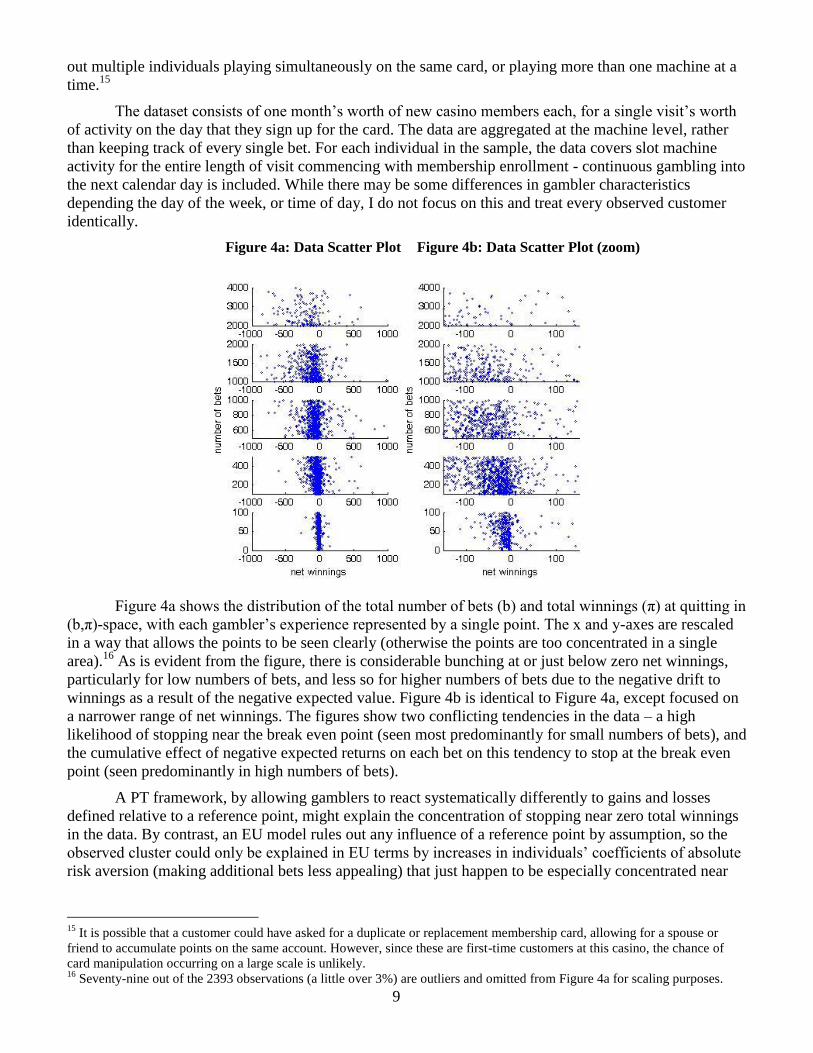
Figure 4a: Data Scatter Plot Figure 4b: Data Scatter Plot (zoom)

Figure 4a shows the distribution of the total number of bets (b) and total winnings (π) at quitting in

(b,π)-space, with each gambler‟s experience represented by a single point. The x and y-axes are rescaled

in a way that allows the points to be seen clearly (otherwise the points are too concentrated in a single

area).16

As is evident from the figure, there is considerable bunching at or just below zero net winnings,

particularly for low numbers of bets, and less so for higher numbers of bets due to the negative drift to

winnings as a result of the negative expected value. Figure 4b is identical to Figure 4a, except focused on

a narrower range of net winnings. The figures show two conflicting tendencies in the data – a high

likelihood of stopping near the break even point (seen most predominantly for small numbers of bets), and

the cumulative effect of negative expected returns on each bet on this tendency to stop at the break even

point (seen predominantly in high numbers of bets).

A PT framework, by allowing gamblers to react systematically differently to gains and losses

defined relative to a reference point, might explain the concentration of stopping near zero total winnings

in the data. By contrast, an EU model rules out any influence of a reference point by assumption, so the

observed cluster could only be explained in EU terms by increases in individuals‟ coefficients of absolute

risk aversion (making additional bets less appealing) that just happen to be especially concentrated near

15

It is possible that a customer could have asked for a duplicate or replacement membership card, allowing for a spouse or

friend to accumulate points on the same account. However, since these are first-time customers at this casino, the chance of

card manipulation occurring on a large scale is unlikely. 16

Seventy-nine out of the 2393 observations (a little over 3%) are outliers and omitted from Figure 4a for scaling purposes.

10

the break-even point despite individual heterogeneity in wealth – an unlikely explanation. This suggests

that PT might explain the patterns in the data more gracefully than EU.

To make this point clearer, imagine that Figure 4 consisted of an extremely concentrated set of

points forming a solid vertical line at the zero net winnings mark (a very extreme version of what the

actual data hint at). This would mean that everybody in the sample had stopped at zero net winnings, no

matter how many bets they had taken. For an Expected Utility framework to explain such behavior, every

person in the sample would have to have a drastic upward spike in risk aversion at exactly zero net

winnings, regardless of their wealth differences. Such uniform stopping would be a huge coincidence.

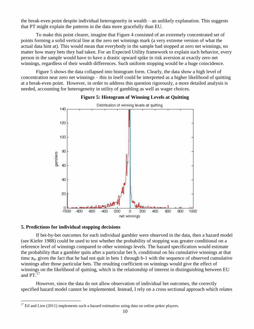
Figure 5 shows the data collapsed into histogram form. Clearly, the data show a high level of

concentration near zero net winnings – this in itself could be interpreted as a higher likelihood of quitting

at a break-even point. However, in order to address this question rigorously, a more detailed analysis is

needed, accounting for heterogeneity in utility of gambling as well as wager choices.

Figure 5: Histogram of Winning Levels at Quitting

5. Predictions for individual stopping decisions

If bet-by-bet outcomes for each individual gambler were observed in the data, then a hazard model

(see Kiefer 1988) could be used to test whether the probability of stopping was greater conditional on a

reference level of winnings compared to other winnings levels. The hazard specification would estimate

the probability that a gambler quits after a particular bet b, conditional on his cumulative winnings at that

time πb, given the fact that he had not quit in bets 1 through b-1 with the sequence of observed cumulative

winnings after those particular bets. The resulting coefficient on winnings would give the effect of

winnings on the likelihood of quitting, which is the relationship of interest in distinguishing between EU

and PT.17

However, since the data do not allow observation of individual bet outcomes, the correctly

specified hazard model cannot be implemented. Instead, I rely on a cross sectional approach which relates

17

Eil and Lien (2011) implements such a hazard estimation using data on online poker players.

11

observed final winnings to the empirical likelihood of quitting, using completely random quitting as the

null hypothesis representing EU. Statistically distinguishing between EU and the deliberate stopping near

the reference point predicted by PT, relies on the independent nature of individual bet outcomes. Slot

machines in the United States have payouts determined by random number generators resulting in bet-by-

bet outcomes which are fully independent of any previous or future bet outcomes (Zangeneh,

Blaszczynski, Turner, 2008, p.18).18

This is the first main assumption needed in order to justify normality

testing as a method for determining whether stopping was non-random, and is clearly satisfied by the slot

machine environment.19

In addition, I need to assume that winnings are drawn from identical distributions in order to

connect gamblers‟ preferences over winnings to the observed cross-sectional distributions of outcomes.

However, distributions of total winnings are generally not identical across gamblers for two main reasons.

First, there is a drift associated with a gambler‟s net winnings depending on how many bets he has taken.

If a single bet has an expected value of μ and a variance of σ2, the sum of outcomes from a sufficiently

large number b of identical bets is approximated by N(μb, σ2b). This means that in the case of negative

expected value bets such as slot machine bets, as a gambler takes more bets, the expectation of his

cumulative winnings is declining and its variance is increasing. In other words, there is both a negative

drift and a spreading out of possible outcomes with each bet taken.

Second, the distribution of possible winnings can differ depending on the gambler‟s chosen wager

size. This is important because assuming that the mean and variance of a single bet remain in

approximately constant proportions for a given wager unit, a gambler taking 5 cent bets has a higher

expected value and lower variance of winnings than a gambler betting 80 cents each time, for an identical

number of bets. A simple way of modeling this potential heterogeneity in bet sizes is to categorize the

distribution of winnings as a function of both number of bets taken b and wager size w, N(wμb, (wσ)2b). I

take w to be an individual gambler‟s average wager during the visit – the ratio of a gambler‟s total amount

wagered over the total number of bets taken.20

So to maintain cross-sectional normality, I need groups of gamblers who are identical across

wager size as well as number of bets taken. In other words, gamblers observed in a single wagers-bets bin

(w,b) should be theoretically indistinguishable from a normal distribution under the EU hypothesis.

However, since the data do not provide enough gamblers in each (w,b) bin to test for normality separately

for each bin, consecutive bins must be combined in order to get a reasonable sample size.21

While this will

technically result in a non-normal distribution, the objective is to combine consecutive bins in such a way

that simulations of winnings drawn from empirical bin frequencies of the relevant normal distributions

18

This was also confirmed by the casino which provided the data for this paper. By contrast slot machines in the United

Kingdom are permitted to have payouts which follow adaptive algorithms, which is beneficial from the point of view of the

casino in that they can ensure a short term profit. Compared to UK machines, US slot machines are completely independent

draws, relying on the law of large numbers for the casino to obtain its expected long run profit. In addition US slot machines

tend to pay out less frequently but in larger amounts when they do. 19

A key point is whether the number of bets taken by individuals in the sample is large enough for their personal theoretical

distribution of cumulative winnings to approximate normality. Appendix D shows the convergence towards a normal

distribution when the underlying payout distribution is shaped like the exponential distribution. For functional simplicity, I will

assume from this point forward that the personal distribution of cumulative winnings conditional on wager size and number of

bets taken has approximately converged to the normal distribution – however lack of full convergence does not adequately

account for the pattern of stopping decisions observed in the data. 20

Within-person wager heterogeneity is unobserved in the data, but under the finite menu of payout distributions in a casino,

survives the CLT through the Lindberg-Feller condition. Meaning with reasonable assumptions on variances of any single bet‟s

distribution, the sum of non-identical but independent bet outcomes will still converge to a normal distribution. 21

An alternative approach would sample and sum a small finite number of individual gamblers‟ final winnings with

replacement from both the simulated normal distributions and the empirical distribution. The empirical distribution of sums

should be normal in the limit under EU, and remain non-normal under PT. However, this appears to be a computationally

intensive approach given the heterogeneity of normal distributions used, and would not be as visually informative about cross-

sectional quitting patterns compared to combining the adjacent (w,b) bins.

12

will be nearly indistinguishable from normality. Applying the same normality test to both the simulated

data and the actual data will then reveal how far from random the quitting behavior in the data were.

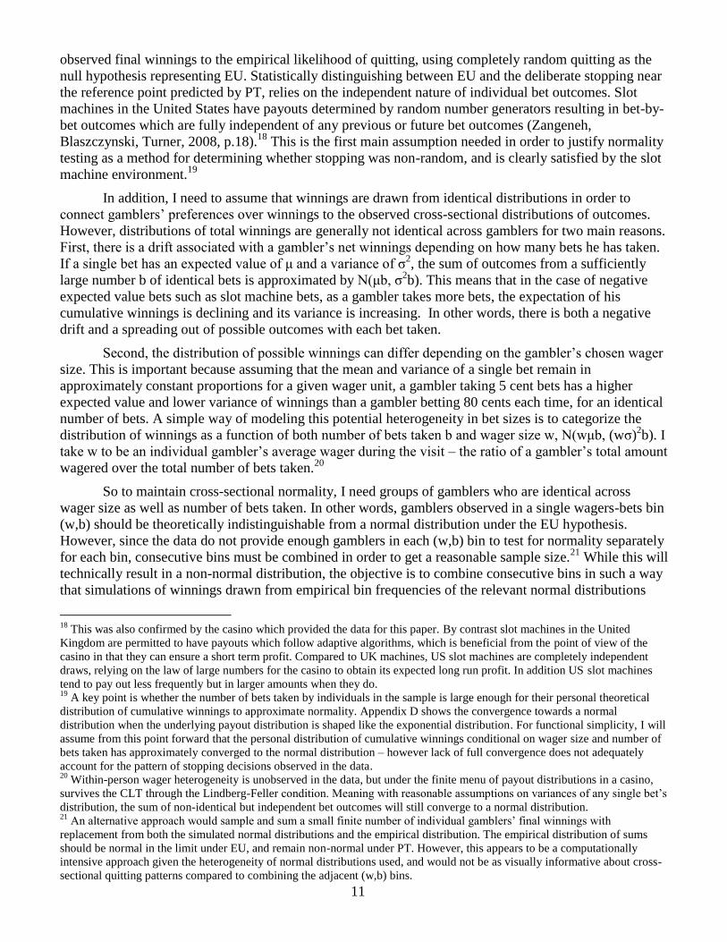
What does it mean to reject normality in the data? First, compared to the normal distribution in

winnings implied by EU, excess kurtosis would imply an unusually high stopping frequency at some

particular level of winnings, which would then be interpreted as the reference point. Figure 6 shows three

distributions of varying kurtosis levels; the distribution on the far right has “excess kurtosis” or higher

kurtosis than a normal distribution.

Figure 6: Illustration of Kurtosis

Negative excess kurtosis Normal distribution Positive excess kurtosis

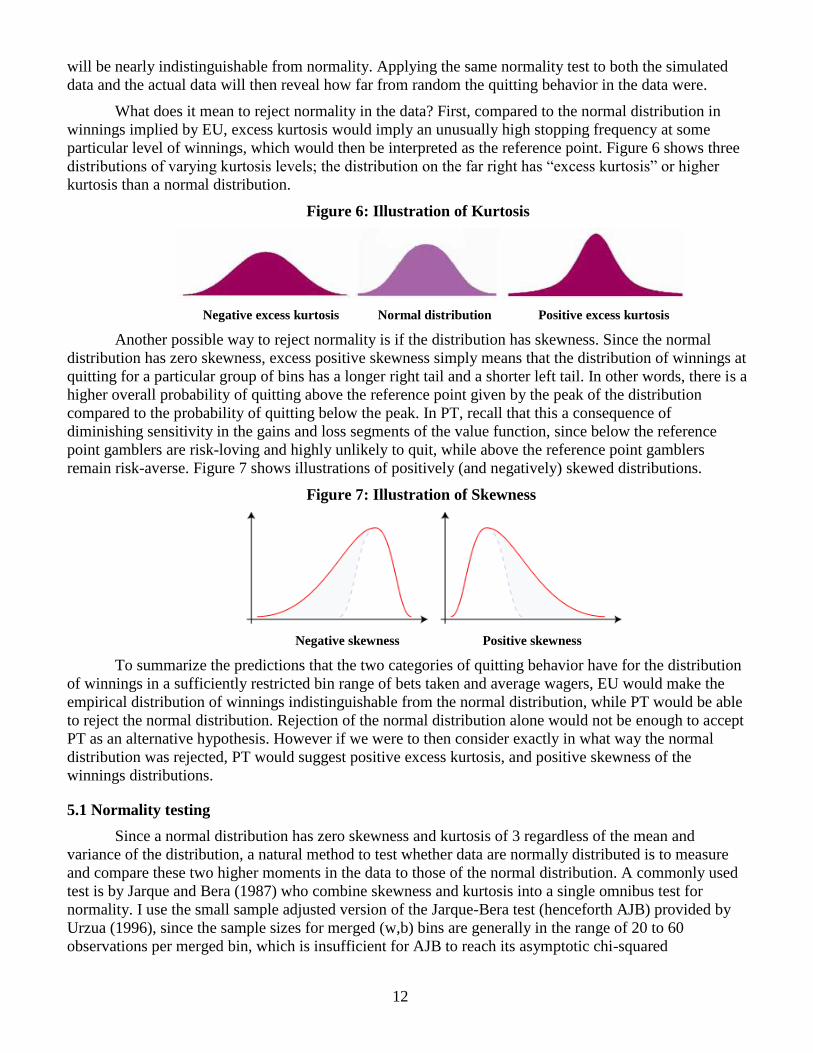
Another possible way to reject normality is if the distribution has skewness. Since the normal

distribution has zero skewness, excess positive skewness simply means that the distribution of winnings at

quitting for a particular group of bins has a longer right tail and a shorter left tail. In other words, there is a

higher overall probability of quitting above the reference point given by the peak of the distribution

compared to the probability of quitting below the peak. In PT, recall that this a consequence of

diminishing sensitivity in the gains and loss segments of the value function, since below the reference

point gamblers are risk-loving and highly unlikely to quit, while above the reference point gamblers

remain risk-averse. Figure 7 shows illustrations of positively (and negatively) skewed distributions.

Figure 7: Illustration of Skewness

Negative skewness Positive skewness

To summarize the predictions that the two categories of quitting behavior have for the distribution

of winnings in a sufficiently restricted bin range of bets taken and average wagers, EU would make the

empirical distribution of winnings indistinguishable from the normal distribution, while PT would be able

to reject the normal distribution. Rejection of the normal distribution alone would not be enough to accept

PT as an alternative hypothesis. However if we were to then consider exactly in what way the normal

distribution was rejected, PT would suggest positive excess kurtosis, and positive skewness of the

winnings distributions.

5.1 Normality testing

Since a normal distribution has zero skewness and kurtosis of 3 regardless of the mean and

variance of the distribution, a natural method to test whether data are normally distributed is to measure

and compare these two higher moments in the data to those of the normal distribution. A commonly used

test is by Jarque and Bera (1987) who combine skewness and kurtosis into a single omnibus test for

normality. I use the small sample adjusted version of the Jarque-Bera test (henceforth AJB) provided by

Urzua (1996), since the sample sizes for merged (w,b) bins are generally in the range of 20 to 60

observations per merged bin, which is insufficient for AJB to reach its asymptotic chi-squared

13

distribution.22

In order to obtain more precise critical values for the AJB test for sample sizes not included

in the table from Urzua (1996), I simulate the 95% critical values for the range of relevant sample sizes.23

Since w is the average wager of an individual gambler, and estimate of the true amount they prefer

to wager on each bet, putting individuals into groups based on consecutive average wagers essentially

groups them by an estimate of their gambling type – for example, “very small stakes” gamblers might be

grouped as those who wagered an average of between one and 20 cents on each bet. “Medium stakes”

gamblers might be defined as those who wagered an average of 40 to 60 cents per bet.

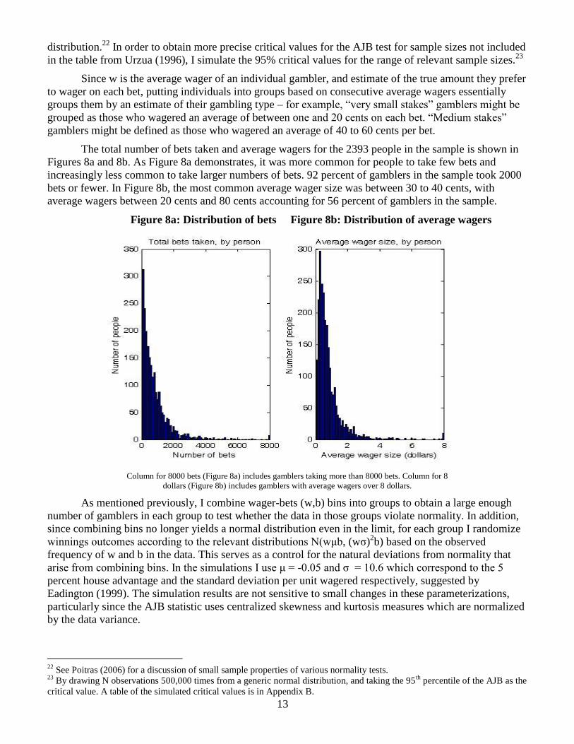
The total number of bets taken and average wagers for the 2393 people in the sample is shown in

Figures 8a and 8b. As Figure 8a demonstrates, it was more common for people to take few bets and

increasingly less common to take larger numbers of bets. 92 percent of gamblers in the sample took 2000

bets or fewer. In Figure 8b, the most common average wager size was between 30 to 40 cents, with

average wagers between 20 cents and 80 cents accounting for 56 percent of gamblers in the sample.

Figure 8a: Distribution of bets Figure 8b: Distribution of average wagers

Column for 8000 bets (Figure 8a) includes gamblers taking more than 8000 bets. Column for 8

dollars (Figure 8b) includes gamblers with average wagers over 8 dollars.

As mentioned previously, I combine wager-bets (w,b) bins into groups to obtain a large enough

number of gamblers in each group to test whether the data in those groups violate normality. In addition,

since combining bins no longer yields a normal distribution even in the limit, for each group I randomize

winnings outcomes according to the relevant distributions N(wμb, (wσ)2b) based on the observed

frequency of w and b in the data. This serves as a control for the natural deviations from normality that

arise from combining bins. In the simulations I use μ = -0.05 and σ = 10.6 which correspond to the 5

percent house advantage and the standard deviation per unit wagered respectively, suggested by

Eadington (1999). The simulation results are not sensitive to small changes in these parameterizations,

particularly since the AJB statistic uses centralized skewness and kurtosis measures which are normalized

by the data variance.

22

See Poitras (2006) for a discussion of small sample properties of various normality tests. 23

By drawing N observations 500,000 times from a generic normal distribution, and taking the 95th

percentile of the AJB as the

critical value. A table of the simulated critical values is in Appendix B.

14

How important is it to account for wager heterogeneity? This is a question of particular interest

since a gambler‟s choice of wager is itself an indicator of risk preferences. If the data tracked the wager

amount for each individual bet, then useful information about the dynamics of risk preferences might

result – for example, I might consistently observe whether a gambler reduced his bet size when

approaching certain (reference) winnings levels. However, since only the average wager for each gambler

is available, the gambler‟s “type” as defined by whether they were a low stakes bettor, high stakes bettor

or somewhere in between, is actually a confounding factor when testing for normality. This is because

heterogeneity in average wagers across gamblers can produce non-normality (via heterogeneous means

and variances) which would be overlooked if wagers were simply averaged across all gamblers.24

Table 1 divides the sample into groups by total number of bets taken in a single visit. The columns

labeled “common wager” show the simulated normality rejection rates, 95th

percentile of skewness and

excess kurtosis respectively, all assuming that gamblers have a common wager equal to the average wager

in the population of 84 cents. The AJB test fails to reject the null hypothesis of normality about 95 percent

of the time for groups with larger number of bets. Skewness and excess kurtosis at the 95th

percentile are

not drastically different from those of the normal distribution. However once the same individuals are

simulated according to their personal average wagers, normality is fully rejected for the exact same

subgroups of gamblers (see far most right 3 columns). This shows that wager heterogeneity cannot be

ignored, and therefore that the groups of gamblers in Table 1 must be broken into even smaller groups by

wager sizes in the main empirical analysis in order to provide a valid simulated control group.

Table 1: Comparison of group rejection of normality with and without wager heterogeneity (simulations only)

from bet to bet

number of

gamblers in group

simulated reject rate of normal

distribution at 95% level

(common wager =

0.84)

95th percentile of group

skewness (common

wager)

95th percentile of group excess kurtosis

(common wager)

simulated reject rate of normal

distribution at 95% level

(personal wager)

95th percentile of group

skewness (personal

wager)

95th percentile of group excess kurtosis

(personal wager)

1 60 222 0.47 0.35 1.79 1 6.61 117.99

61 130 222 0.11 0.29 0.91 1 2.01 23.91

131 210 203 0.08 0.29 0.76 1 4.84 76.25

211 300 202 0.06 0.26 0.68 1 3.30 39.03

301 410 203 0.06 0.30 0.65 1 7.96 125.72

411 540 200 0.06 0.30 0.62 1 2.32 34.88

541 700 203 0.05 0.29 0.60 1 3.44 51.54

701 870 202 0.05 0.27 0.62 1 2.30 32.47

871 1120 204 0.06 0.28 0.64 1 2.96 42.65

1121 1520 202 0.06 0.30 0.70 1 0.94 12.82

1521 2490 200 0.07 0.29 0.69 1 5.29 84.93

2491 14370 130 0.40 0.33 2.98 1 1.89 30.54

Number of bets grouped so as to have at least 200 gamblers per group. Columns 4 through 6 (common wager) are simulated

using N(0.84*μb, (0.84σ)2b*) with empirical b frequencies. Columns 7 through 9 (personal wager) are simulated using N(wμb,

(wσ)2b) with empirical b and w frequencies. 1000 simulations for each group.

6. Results

Table 2 shows a comparison of the simulated winnings distribution for each group of combined

bins, and the AJB statistic for each corresponding group in the data. The simulated reject rate is typically

near or slightly above 5 percent using the 95 percent critical values estimated in Appendix B. As in Table

24

For example two normal distributions with the same mean but different variances tend to produce excess kurtosis. Two

normal distributions with very different means tend to produce a distribution with two peaks, and so on.

15

1, the reject rate is substantially higher for simulations for small numbers of bets (bets 1 to 60), which is

consistent with the CLT.

The four columns on the far right of Table 2 compare the 95th

percentile of the simulated excess

skewness and kurtosis values to the values of these moments in the data. The simulated 95th

percentile of

skewness column shows that there is some positive skewness that results purely from combining adjacent

bins – however in cases where the data rejects normality, the data tend to be skewed even farther to the

right than the simulations. The story is similar for kurtosis levels. There is a natural tendency for quitting

to bunch near certain winnings levels due to merging the bins, however in groups where normality is

rejected in the data, the bunching point-wise exceeds the levels implied by the simulations.

Table 2: Normality tests by number of bets and average wager types

from bet to bet

from average wager

(dollars)

to average wager

(dollars)

number of

gamblers in group

simulated reject rate of normal

distribution at 95% critical value

AJB statistic (data)

indicator for

rejection of normal

distribution in data at 95% level

simulated 95th

percentile of

skewness data

skewness

simulated 95th

percentile of excess kurtosis

data excess kurtosis

1 60 0.21 0.40 43 0.20 9.40 1 0.83 0.17 2.89 2.15

1 60 0.41 0.60 30 0.15 38.28 1 0.95 1.89** 2.82 3.59**

1 60 0.61 0.80 36 0.17 1586.31 1 0.90 5.16** 3.03 28.88**

61 130 0.21 0.40 50 0.12 41.81 1 0.62 1.41** 2.18 3.27**

61 130 0.41 0.60 49 0.09 1.32 0 0.64 0.00 1.71 0.77

61 130 0.61 0.80 33 0.08 66.98 1 0.78 2.16** 2.10 4.99**

131 210 0.21 0.40 37 0.12 3.81 0 0.78 0.74 2.21 0.27

131 210 0.41 0.60 41 0.07 4.77 0 0.67 0.37 1.65 1.41

131 210 0.61 0.80 26 0.05 15.34 1 0.78 1.06** 1.86 2.79**

211 300 0.21 0.40 43 0.09 29.85 1 0.67 1.45** 1.87 2.63**

211 300 0.41 0.60 34 0.08 200.04 1 0.74 2.89** 1.88 9.61**

211 300 0.61 0.80 26 0.07 1.95 0 0.80 -0.57 2.18 0.53

301 410 0.21 0.40 49 0.12 1.06 0 0.68 0.18 2.03 0.59

301 410 0.41 0.60 39 0.08 47.13 1 0.64 1.69** 1.76 3.86**

301 410 0.61 0.80 31 0.06 85.94 1 0.66 2.33** 1.64 6.11**

411 540 0.21 0.40 45 0.087 58.84 1 0.60 1.20** 1.83 4.77**

411 540 0.41 0.60 36 0.061 840.02 1 0.65 4.08** 1.81 20.78**

411 540 0.61 0.80 31 0.06 200.30 1 0.73 2.76** 1.87 10.29**

541 700 0.21 0.40 48 0.11 42.52 1 0.66 1.30** 1.91 3.58**

541 700 0.41 0.60 47 0.067 86.99 1 0.59 1.85** 1.56 5.21**

541 700 0.61 0.80 22 0.054 126.18 1 0.82 2.60** 1.94 9.44**

701 870 0.21 0.40 53 0.105 63.03 1 0.62 1.54** 2.00 4.12**

701 870 0.41 0.60 37 0.06 1.22 0 0.60 0.11 1.59 0.81

701 870 0.61 0.80 34 0.052 63.94 1 0.65 1.89** 1.65 5.10**

871 1120 0.21 0.40 47 0.116 0.99 0 0.66 0.06 2.11 -0.67

871 1120 0.41 0.60 37 0.075 178.22 1 0.69 2.35** 1.84 9.02**

871 1120 0.61 0.80 37 0.079 154.53 1 0.70 2.33** 1.84 8.26**

1121 1520 0.21 0.40 44 0.099 3.58 0 0.65 0.29 1.98 1.20

1121 1520 0.41 0.60 35 0.074 27.25 1 0.69 1.20** 1.88 3.31**

1121 1520 0.61 0.80 32 0.062 5.34 0 0.69 0.62 1.75 1.43

1521 2490 0.21 0.40 46 0.093 11.53 1 0.63 0.47 1.77 2.15

1521 2490 0.41 0.60 44 0.092 20.87 1 0.68 1.35** 1.79 1.79

1521 2490 0.61 0.80 28 0.055 12.52 1 0.75 1.15** 1.78 2.05

Simulations repeated 1000 times for each bin, drawing from N(wμb, (wσ)2b) using empirical b and w frequencies, and μ = -0.05, σ = 10.6

(Eadington 1999). ** indicates deviation from simulated data at the 95th percentile in direction predicted by PT. Results shown in Table for

modal (most frequently occurring) wager categories. See Appendix C for full table with all bins included.

16

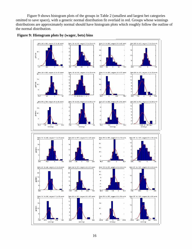
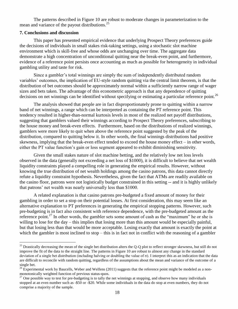
Figure 9 shows histogram plots of the groups in Table 2 (smallest and largest bet categories

omitted to save space), with a generic normal distribution fit overlaid in red. Groups whose winnings

distributions are approximately normal should have histogram plots which roughly follow the outline of

the normal distribution.

Figure 9: Histogram plots by (wager, bets) bins

17

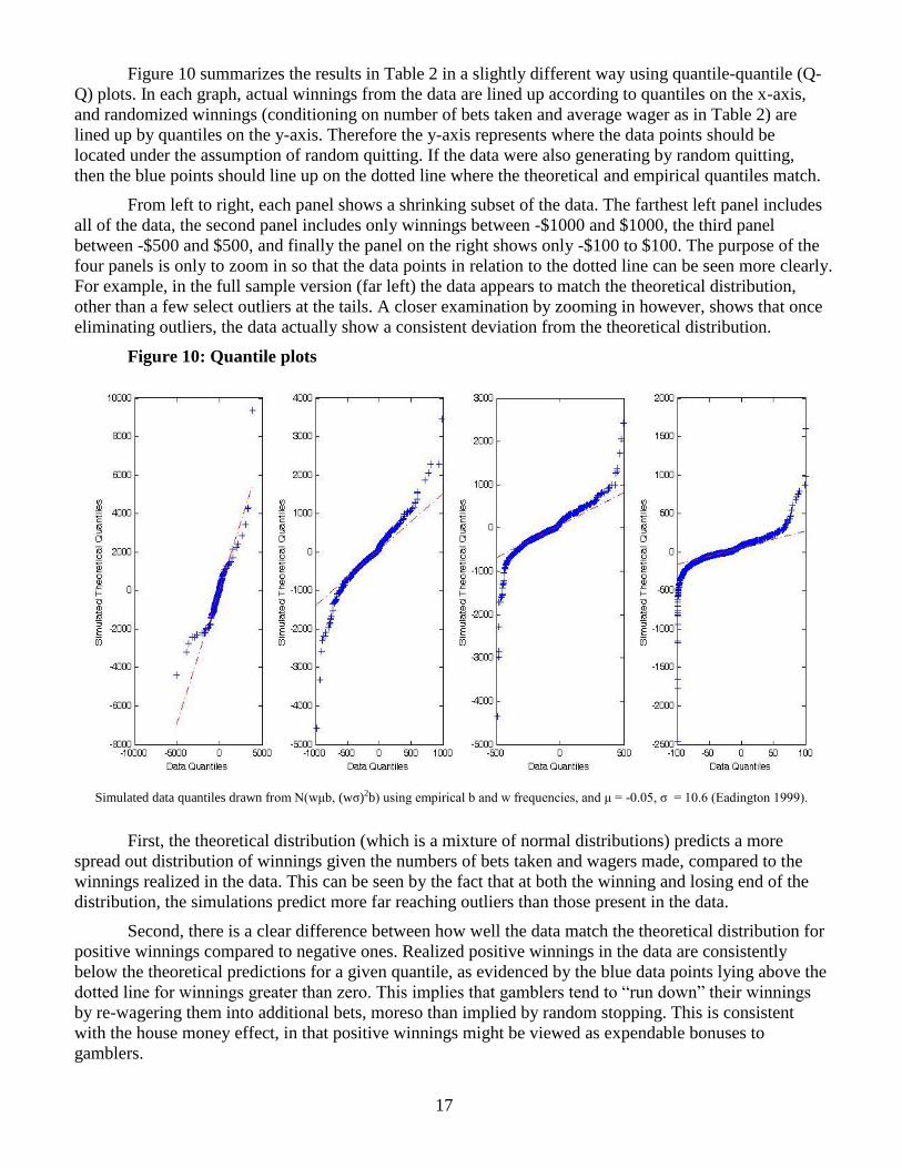
Figure 10 summarizes the results in Table 2 in a slightly different way using quantile-quantile (Q-

Q) plots. In each graph, actual winnings from the data are lined up according to quantiles on the x-axis,

and randomized winnings (conditioning on number of bets taken and average wager as in Table 2) are

lined up by quantiles on the y-axis. Therefore the y-axis represents where the data points should be

located under the assumption of random quitting. If the data were also generating by random quitting,

then the blue points should line up on the dotted line where the theoretical and empirical quantiles match.

From left to right, each panel shows a shrinking subset of the data. The farthest left panel includes

all of the data, the second panel includes only winnings between -$1000 and $1000, the third panel

between -$500 and $500, and finally the panel on the right shows only -$100 to $100. The purpose of the

four panels is only to zoom in so that the data points in relation to the dotted line can be seen more clearly.

For example, in the full sample version (far left) the data appears to match the theoretical distribution,

other than a few select outliers at the tails. A closer examination by zooming in however, shows that once

eliminating outliers, the data actually show a consistent deviation from the theoretical distribution.

Figure 10: Quantile plots

Simulated data quantiles drawn from N(wμb, (wσ)2b) using empirical b and w frequencies, and μ = -0.05, σ = 10.6 (Eadington 1999).

First, the theoretical distribution (which is a mixture of normal distributions) predicts a more

spread out distribution of winnings given the numbers of bets taken and wagers made, compared to the

winnings realized in the data. This can be seen by the fact that at both the winning and losing end of the

distribution, the simulations predict more far reaching outliers than those present in the data.

Second, there is a clear difference between how well the data match the theoretical distribution for

positive winnings compared to negative ones. Realized positive winnings in the data are consistently

below the theoretical predictions for a given quantile, as evidenced by the blue data points lying above the

dotted line for winnings greater than zero. This implies that gamblers tend to “run down” their winnings

by re-wagering them into additional bets, moreso than implied by random stopping. This is consistent

with the house money effect, in that positive winnings might be viewed as expendable bonuses to

gamblers.

18

The patterns described in Figure 10 are robust to moderate changes in parameterization to the

mean and variance of the payout distributions.25

7. Conclusions and discussion

This paper has presented empirical evidence that underlying Prospect Theory preferences guide

the decisions of individuals in small stakes risk-taking settings, using a stochastic slot machine

environment which is skill-free and whose odds are unchanging over time. The aggregate data

demonstrate a high concentration of unconditional quitting near the break-even point, and furthermore,

evidence of a reference point persists once accounting as much as possible for heterogeneity in individual

gambling utility and taste for risk.

Since a gambler‟s total winnings are simply the sum of independently distributed random

variables‟ outcomes, the implication of EU-style random quitting via the central limit theorem, is that the

distribution of bet outcomes should be approximately normal within a sufficiently narrow range of wager

sizes and bets taken. The advantage of this econometric approach is that any dependence of quitting

decisions on net winnings can be identified without specifying or estimating a particular reference point.26

The analysis showed that people are in fact disproportionately prone to quitting within a narrow

band of net winnings, a range which can be interpreted as containing the PT reference point. This

tendency resulted in higher-than-normal kurtosis levels in most of the realized net payoff distributions,

suggesting that gamblers valued their winnings according to Prospect Theory preferences, subscribing to

the house money and break-even effects. Furthermore, based on the distributions of realized winnings,

gamblers were more likely to quit when above the reference point suggested by the peak of the

distribution, compared to quitting below it. In other words, the final winnings distributions had positive

skewness, implying that the break-even effect tended to exceed the house money effect – in other words,

either the PT value function‟s gain or loss segment appeared to exhibit diminishing sensitivity.

Given the small stakes nature of slot machine betting, and the relatively low net loss levels

observed in the data (generally not exceeding a net loss of $1000), it is difficult to believe that net wealth

liquidity constraints played a compelling role in generating the empirical results. However, without

knowing the true distribution of net wealth holdings among the casino patrons, this data cannot directly

refute a liquidity constraint hypothesis. Nevertheless, given the fact that ATMs are readily available on

the casino floor, patrons were not logistically budget constrained in this setting -- and it is highly unlikely

that patrons‟ net wealth was nearly universally less than $1000.

A related explanation is that casino patrons pre-budgeted a fixed amount of money for their

gambling in order to set a stop on their potential losses. At first consideration, this may seem like an

alternative explanation to PT preferences in generating the empirical stopping patterns. However, such

pre-budgeting is in fact also consistent with reference dependence, with the pre-budgeted amount as the

reference point.27

In other words, the gambler sets some amount of cash as the “maximum” he or she is

willing to lose for the day – this implies that losing more than this amount would be especially painful,

but that losing less than that would be more acceptable. Losing exactly that amount is exactly the point at

which the gambler is most inclined to stop – this is in fact not in conflict with the reasoning of a gambler

25

Drastically decreasing the mean of the single bet distribution alters the Q-Q plot to reflect stronger skewness, but still do not

improve the fit of the data to the straight line. The patterns in Figure 10 are robust to almost any change in the standard

deviation of a single bet distribution (including halving or doubling the value of σ). I interpret this as an indication that the data

are difficult to reconcile with random quitting, regardless of the assumptions about the mean and variance of the outcome of a

single bet. 26

Experimental work by Baucells, Weber and Welfens (2011) suggests that the reference point might be modeled as a non-

monotonically weighted function of previous status-quos. 27

One possible way to test for pre-budgeting is to tally the net winnings at stopping, and observe how many individuals

stopped at an even number such as -$50 or -$20. While some individuals in the data do stop at even numbers, they do not

comprise a majority of the sample.

19

who has reference dependent preferences. Further research would be needed to definitively test whether

reference-dependence or other possible factors are in fact behind such “rule of thumb” pre-budgeting

behavior.

Finally, this study has lacked the data to properly account for gamblers‟ beliefs – only partially

addressing the issue by separately examining those gamblers who took many bets (large b bins), which

should give them the chance to learn the payout-generating process. However, the task of thoroughly

separating belief-driven behavior from preference-driven behavior should be more adequately addressed

using a laboratory experiment. I postpone this possibility to further research.

20

References:

Barberis, N. “A Model of Casino Gambling”, Working Paper, March 2009.

Barberis, N., and Xiong, W. “What Drives the Disposition Effect? An Analysis of a Long-Standing

Preference-Based Explanation” NBER Working Paper No. 12397, July 2006.

Baucells, M., Weber, M. and Welfens, F. “Reference-Point Formation and Updating,” Management

Science, Vol. 57, No.3, March 2011, pp. 506-519.

Berger, J. and Pope, D.G. “Can Losing Lead to Winning?” Working paper, August 2009.

Camerer, C. “Prospect Theory in the Wild: Evidence from the Field”, Caltech Social Science Working

Paper 1037, May 1998.

Camerer, C., Babcock, L., Loewenstein, G., and Thaler, R. “Labor Supply of New York City Cabdrivers:

One Day at a Time” The Quarterly Journal of Economics, May 1997, p. 407 - 441.

Conlisk, J. “The Utility of Gambling” Journal of Risk and Uncertainty, 6:255-275 (1993).

Crawford, V.P., and Meng, J.J. “New York City Cabdrivers‟ Labor Supply Revisited: Reference-

Dependent Preferences with Rational-Expectations Targets for Hours and Income,” American Economic

Review 101 (August 2011), p. 1912-1932.

Deb, P., and Sefton, M. “The distribution of a Lagrange multiplier test of normality” Economics Letters

51, (1996) p. 123 – 130.

Eadington, W.R. “The Economics of Casino Gambling” The Journal of Economic Perspectives, Vol. 13,

No. 3 (Summer 1999) pp. 173-192.

Eil. D., and Lien, J. “Staying Ahead and Getting Even: Risk Preferences of Profitable Poker Players”,

Working Paper (2011).

Farber, H.S., “Is Tomorrow Another Day? The Labor Supply of New York City Cabdrivers” Journal of

Political Economy, Vol. 113, No. 1, 2005, p. 46 – 82.

Farber, H.S., “Reference-Dependent Preferences and Labor Supply: The Case of New York City Taxi

Drivers” American Economic Review, 98:3, June 2008, p.1069 - 1082.

Genesove, D., and Mayer, C. “Loss Aversion and Seller Behavior: Evidence from the Housing Market”

Quarterly Journal of Economics, November 2001, p.1233 - 1260.

Jarque, C.M., Bera, A.K. “A Test for Normality of Observations and Regression Residuals” International

Statistical Review, Vol. 55, No.2 (Aug 1987), pp.163 – 172.

Kahneman D., and A. Tversky. “Prospect Theory: An Analysis of Decision Under Risk” Econometrica,

Vol. 47, No. 2, March 1979, p. 263-291.

Kiefer, N.M., “Economic Duration Data and Hazard Functions” Journal of Economic Literature, Vol.

XXVI, June 1988, p. 646-679.

21

Koszegi, B., and Rabin, M. ”A Model of Reference-Dependent Preferences” The Quarterly Journal of

Economics, Vol. CXXI, Issue 4, November 2006, p. 1133 – 1165.

Koszegi, B., and Rabin, M. ”Reference-Dependent Risk Attitudes” American Economic Review, Vol. 97,

No. 4, September 2007, p. 1047 – 1073.

List, J.A., “Neoclassical Theory versus Prospect Theory: Evidence from the Marketplace”, Econometrica,

Vol. 72, No. 2, March 2004, p. 615 – 625.

Odean, T., “Are Investors Reluctant to Realize Their Losses?” The Journal of Finance, Vol. LIII, No. 5,

October 1998, p.1775 – 1798.

Poitras, G., “More of the correct use of omnibus tests for normality” Economics Letters 90 (2006), p.304

– 309.

Pope, D. and Schweitzer, M.E., “Is Tiger Woods Loss Averse? Persistent Bias in the Face of Experience,

Competition, and High Stakes”, American Economic Review, forthcoming.

Post, T., van den Assem, M.J., Baltussen, G., and Thaler, R.H. “Deal or No Deal? Decision Making under

Risk in a Large-Payoff Game Show” American Economic Review, Vol. 98, No. 1, 2008, p. 38-71.

Rabin, M. “Risk Aversion and Expected-Utility Theory: A Calibration Theorem” Econometrica, Vol. 68,

No.5, Sept. 2000, p.1281-1292.

Rabin, M., and R.H. Thaler. “Anomalies: Risk Aversion” Journal of Economic Perspectives. Vol. 15,

No.1, Winter 2001, p. 219 - 232.

Segal, U. and Spivak, A. “First Order versus Second Order Risk Aversion” Journal of Economic Theory,

51, 111-125 (1990), 111-125.

Thaler, R. and E. Johnson. “Gambling with the House Money and Trying to Break Even: The Effects of

Prior Outcomes on Risky Choice” Management Science, Vol. 36, No. 6, June 1990, p. 643-660.

Urzua, C.M., “On the correct use of omnibus tests for normality” Economics Letters 53 (1996), p.247-251.

Weber, M. and Camerer, C.F., “The disposition effect in securities trading: an experimental analysis,”

Journal of Economic Behavior and Organization, Vol. 33 (1998), p.167-184.

Wooldridge, J.M. Econometric Analysis of Cross Section and Panel Data, MIT Press, 2002.

Zangeneh, M., Blaszczynski, A., Turner, N.E., In the Pursuit of Winning: Problem Gambling Theory,

Research and Treatment, “Chapter 2: Explaining Why People Gamble” by Walker, M., Schellink, T. and

Anjoul, F.

22

Appendix A: List of acronyms and variables

EU = Expected Utility

PT = Prospect Theory

CLT = central limit theorem

AJB = size adjusted Jarque-Bera test

b = total bets taken by gambler

w = gambler‟s average wager

μ = per unit mean of slot machine payout distribution

σ = per unit standard deviation of slot machine payout distribution

π = gambler‟s net winnings for entire visit

23

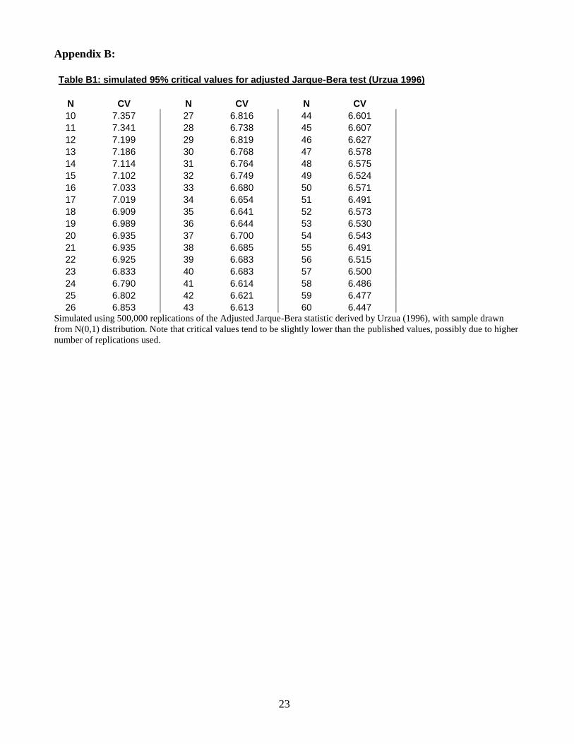
Appendix B:

Table B1: simulated 95% critical values for adjusted Jarque-Bera test (Urzua 1996)

N CV N CV N CV

10 7.357 27 6.816 44 6.601

11 7.341 28 6.738 45 6.607

12 7.199 29 6.819 46 6.627

13 7.186 30 6.768 47 6.578

14 7.114 31 6.764 48 6.575

15 7.102 32 6.749 49 6.524

16 7.033 33 6.680 50 6.571

17 7.019 34 6.654 51 6.491

18 6.909 35 6.641 52 6.573

19 6.989 36 6.644 53 6.530

20 6.935 37 6.700 54 6.543

21 6.935 38 6.685 55 6.491

22 6.925 39 6.683 56 6.515

23 6.833 40 6.683 57 6.500

24 6.790 41 6.614 58 6.486

25 6.802 42 6.621 59 6.477

26 6.853 43 6.613 60 6.447 Simulated using 500,000 replications of the Adjusted Jarque-Bera statistic derived by Urzua (1996), with sample drawn

from N(0,1) distribution. Note that critical values tend to be slightly lower than the published values, possibly due to higher

number of replications used.

24

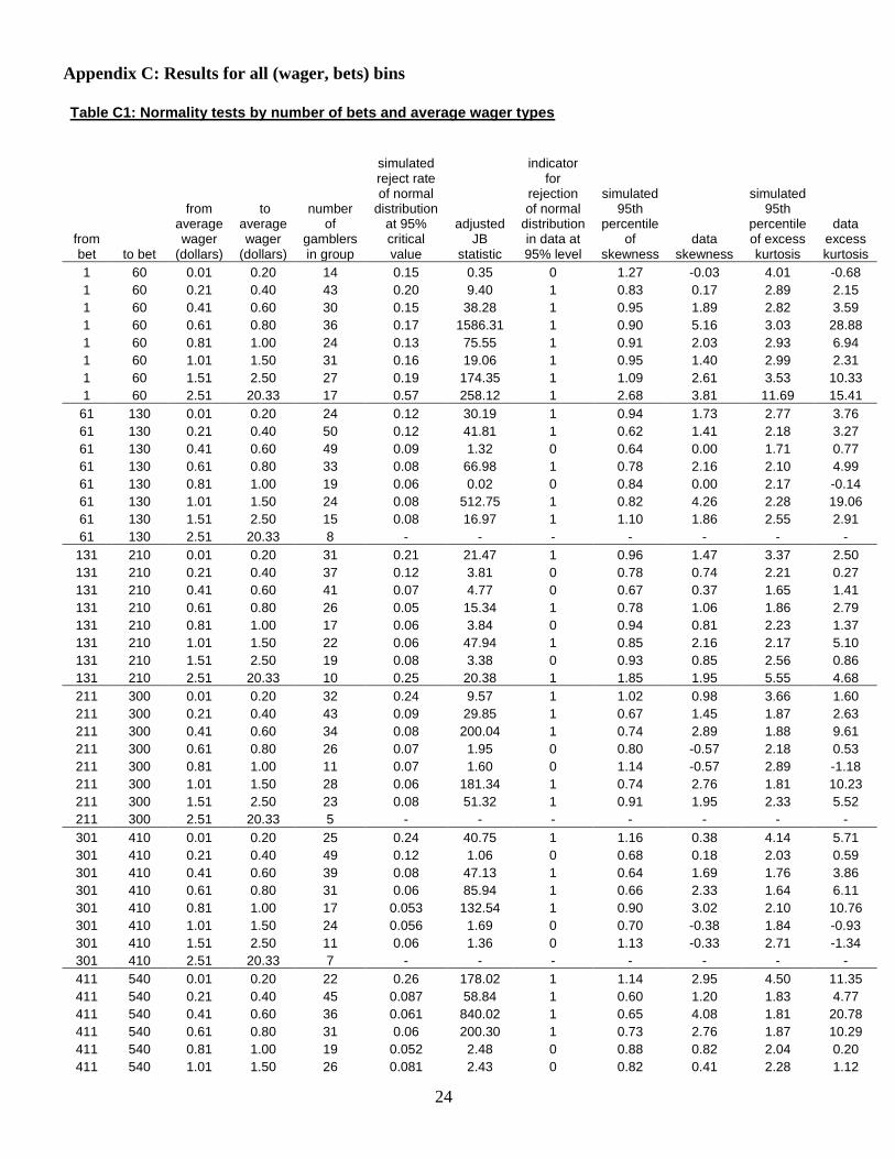
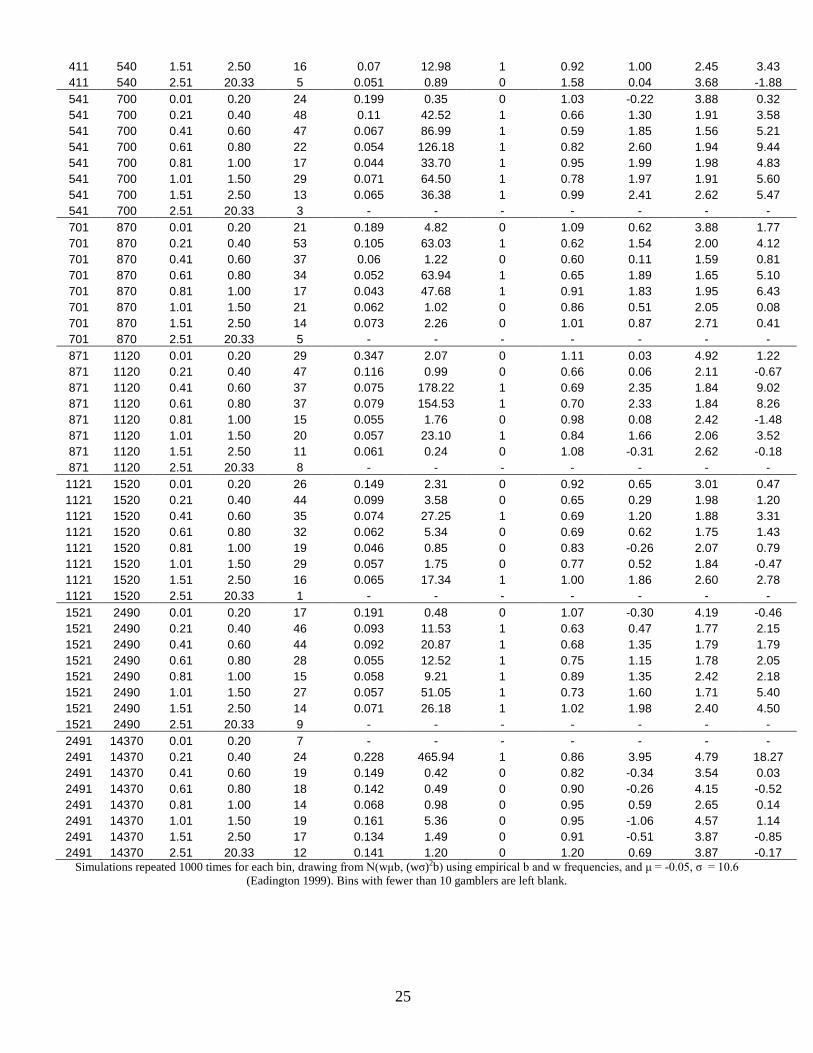
Appendix C: Results for all (wager, bets) bins Table C1: Normality tests by number of bets and average wager types

from bet to bet

from average wager

(dollars)

to average wager

(dollars)

number of

gamblers in group

simulated reject rate of normal

distribution at 95% critical value

adjusted JB

statistic

indicator for

rejection of normal

distribution in data at 95% level

simulated 95th

percentile of

skewness data

skewness

simulated 95th

percentile of excess kurtosis

data excess kurtosis

1 60 0.01 0.20 14 0.15 0.35 0 1.27 -0.03 4.01 -0.68

1 60 0.21 0.40 43 0.20 9.40 1 0.83 0.17 2.89 2.15

1 60 0.41 0.60 30 0.15 38.28 1 0.95 1.89 2.82 3.59

1 60 0.61 0.80 36 0.17 1586.31 1 0.90 5.16 3.03 28.88

1 60 0.81 1.00 24 0.13 75.55 1 0.91 2.03 2.93 6.94

1 60 1.01 1.50 31 0.16 19.06 1 0.95 1.40 2.99 2.31

1 60 1.51 2.50 27 0.19 174.35 1 1.09 2.61 3.53 10.33

1 60 2.51 20.33 17 0.57 258.12 1 2.68 3.81 11.69 15.41

61 130 0.01 0.20 24 0.12 30.19 1 0.94 1.73 2.77 3.76

61 130 0.21 0.40 50 0.12 41.81 1 0.62 1.41 2.18 3.27

61 130 0.41 0.60 49 0.09 1.32 0 0.64 0.00 1.71 0.77

61 130 0.61 0.80 33 0.08 66.98 1 0.78 2.16 2.10 4.99

61 130 0.81 1.00 19 0.06 0.02 0 0.84 0.00 2.17 -0.14

61 130 1.01 1.50 24 0.08 512.75 1 0.82 4.26 2.28 19.06

61 130 1.51 2.50 15 0.08 16.97 1 1.10 1.86 2.55 2.91

61 130 2.51 20.33 8 - - - - - - -

131 210 0.01 0.20 31 0.21 21.47 1 0.96 1.47 3.37 2.50

131 210 0.21 0.40 37 0.12 3.81 0 0.78 0.74 2.21 0.27

131 210 0.41 0.60 41 0.07 4.77 0 0.67 0.37 1.65 1.41

131 210 0.61 0.80 26 0.05 15.34 1 0.78 1.06 1.86 2.79

131 210 0.81 1.00 17 0.06 3.84 0 0.94 0.81 2.23 1.37

131 210 1.01 1.50 22 0.06 47.94 1 0.85 2.16 2.17 5.10

131 210 1.51 2.50 19 0.08 3.38 0 0.93 0.85 2.56 0.86

131 210 2.51 20.33 10 0.25 20.38 1 1.85 1.95 5.55 4.68

211 300 0.01 0.20 32 0.24 9.57 1 1.02 0.98 3.66 1.60

211 300 0.21 0.40 43 0.09 29.85 1 0.67 1.45 1.87 2.63

211 300 0.41 0.60 34 0.08 200.04 1 0.74 2.89 1.88 9.61

211 300 0.61 0.80 26 0.07 1.95 0 0.80 -0.57 2.18 0.53

211 300 0.81 1.00 11 0.07 1.60 0 1.14 -0.57 2.89 -1.18

211 300 1.01 1.50 28 0.06 181.34 1 0.74 2.76 1.81 10.23

211 300 1.51 2.50 23 0.08 51.32 1 0.91 1.95 2.33 5.52

211 300 2.51 20.33 5 - - - - - - -

301 410 0.01 0.20 25 0.24 40.75 1 1.16 0.38 4.14 5.71

301 410 0.21 0.40 49 0.12 1.06 0 0.68 0.18 2.03 0.59

301 410 0.41 0.60 39 0.08 47.13 1 0.64 1.69 1.76 3.86

301 410 0.61 0.80 31 0.06 85.94 1 0.66 2.33 1.64 6.11

301 410 0.81 1.00 17 0.053 132.54 1 0.90 3.02 2.10 10.76

301 410 1.01 1.50 24 0.056 1.69 0 0.70 -0.38 1.84 -0.93

301 410 1.51 2.50 11 0.06 1.36 0 1.13 -0.33 2.71 -1.34

301 410 2.51 20.33 7 - - - - - - -

411 540 0.01 0.20 22 0.26 178.02 1 1.14 2.95 4.50 11.35

411 540 0.21 0.40 45 0.087 58.84 1 0.60 1.20 1.83 4.77

411 540 0.41 0.60 36 0.061 840.02 1 0.65 4.08 1.81 20.78

411 540 0.61 0.80 31 0.06 200.30 1 0.73 2.76 1.87 10.29

411 540 0.81 1.00 19 0.052 2.48 0 0.88 0.82 2.04 0.20

411 540 1.01 1.50 26 0.081 2.43 0 0.82 0.41 2.28 1.12

25

411 540 1.51 2.50 16 0.07 12.98 1 0.92 1.00 2.45 3.43

411 540 2.51 20.33 5 0.051 0.89 0 1.58 0.04 3.68 -1.88

541 700 0.01 0.20 24 0.199 0.35 0 1.03 -0.22 3.88 0.32

541 700 0.21 0.40 48 0.11 42.52 1 0.66 1.30 1.91 3.58

541 700 0.41 0.60 47 0.067 86.99 1 0.59 1.85 1.56 5.21

541 700 0.61 0.80 22 0.054 126.18 1 0.82 2.60 1.94 9.44

541 700 0.81 1.00 17 0.044 33.70 1 0.95 1.99 1.98 4.83

541 700 1.01 1.50 29 0.071 64.50 1 0.78 1.97 1.91 5.60

541 700 1.51 2.50 13 0.065 36.38 1 0.99 2.41 2.62 5.47

541 700 2.51 20.33 3 - - - - - - -

701 870 0.01 0.20 21 0.189 4.82 0 1.09 0.62 3.88 1.77

701 870 0.21 0.40 53 0.105 63.03 1 0.62 1.54 2.00 4.12

701 870 0.41 0.60 37 0.06 1.22 0 0.60 0.11 1.59 0.81

701 870 0.61 0.80 34 0.052 63.94 1 0.65 1.89 1.65 5.10

701 870 0.81 1.00 17 0.043 47.68 1 0.91 1.83 1.95 6.43

701 870 1.01 1.50 21 0.062 1.02 0 0.86 0.51 2.05 0.08

701 870 1.51 2.50 14 0.073 2.26 0 1.01 0.87 2.71 0.41

701 870 2.51 20.33 5 - - - - - - -

871 1120 0.01 0.20 29 0.347 2.07 0 1.11 0.03 4.92 1.22

871 1120 0.21 0.40 47 0.116 0.99 0 0.66 0.06 2.11 -0.67

871 1120 0.41 0.60 37 0.075 178.22 1 0.69 2.35 1.84 9.02

871 1120 0.61 0.80 37 0.079 154.53 1 0.70 2.33 1.84 8.26

871 1120 0.81 1.00 15 0.055 1.76 0 0.98 0.08 2.42 -1.48

871 1120 1.01 1.50 20 0.057 23.10 1 0.84 1.66 2.06 3.52

871 1120 1.51 2.50 11 0.061 0.24 0 1.08 -0.31 2.62 -0.18

871 1120 2.51 20.33 8 - - - - - - -

1121 1520 0.01 0.20 26 0.149 2.31 0 0.92 0.65 3.01 0.47

1121 1520 0.21 0.40 44 0.099 3.58 0 0.65 0.29 1.98 1.20

1121 1520 0.41 0.60 35 0.074 27.25 1 0.69 1.20 1.88 3.31

1121 1520 0.61 0.80 32 0.062 5.34 0 0.69 0.62 1.75 1.43

1121 1520 0.81 1.00 19 0.046 0.85 0 0.83 -0.26 2.07 0.79

1121 1520 1.01 1.50 29 0.057 1.75 0 0.77 0.52 1.84 -0.47

1121 1520 1.51 2.50 16 0.065 17.34 1 1.00 1.86 2.60 2.78

1121 1520 2.51 20.33 1 - - - - - - -

1521 2490 0.01 0.20 17 0.191 0.48 0 1.07 -0.30 4.19 -0.46

1521 2490 0.21 0.40 46 0.093 11.53 1 0.63 0.47 1.77 2.15

1521 2490 0.41 0.60 44 0.092 20.87 1 0.68 1.35 1.79 1.79

1521 2490 0.61 0.80 28 0.055 12.52 1 0.75 1.15 1.78 2.05

1521 2490 0.81 1.00 15 0.058 9.21 1 0.89 1.35 2.42 2.18

1521 2490 1.01 1.50 27 0.057 51.05 1 0.73 1.60 1.71 5.40

1521 2490 1.51 2.50 14 0.071 26.18 1 1.02 1.98 2.40 4.50

1521 2490 2.51 20.33 9 - - - - - - -

2491 14370 0.01 0.20 7 - - - - - - -

2491 14370 0.21 0.40 24 0.228 465.94 1 0.86 3.95 4.79 18.27

2491 14370 0.41 0.60 19 0.149 0.42 0 0.82 -0.34 3.54 0.03

2491 14370 0.61 0.80 18 0.142 0.49 0 0.90 -0.26 4.15 -0.52

2491 14370 0.81 1.00 14 0.068 0.98 0 0.95 0.59 2.65 0.14

2491 14370 1.01 1.50 19 0.161 5.36 0 0.95 -1.06 4.57 1.14

2491 14370 1.51 2.50 17 0.134 1.49 0 0.91 -0.51 3.87 -0.85

2491 14370 2.51 20.33 12 0.141 1.20 0 1.20 0.69 3.87 -0.17

Simulations repeated 1000 times for each bin, drawing from N(wμb, (wσ)2b) using empirical b and w frequencies, and μ = -0.05, σ = 10.6

(Eadington 1999). Bins with fewer than 10 gamblers are left blank.

26

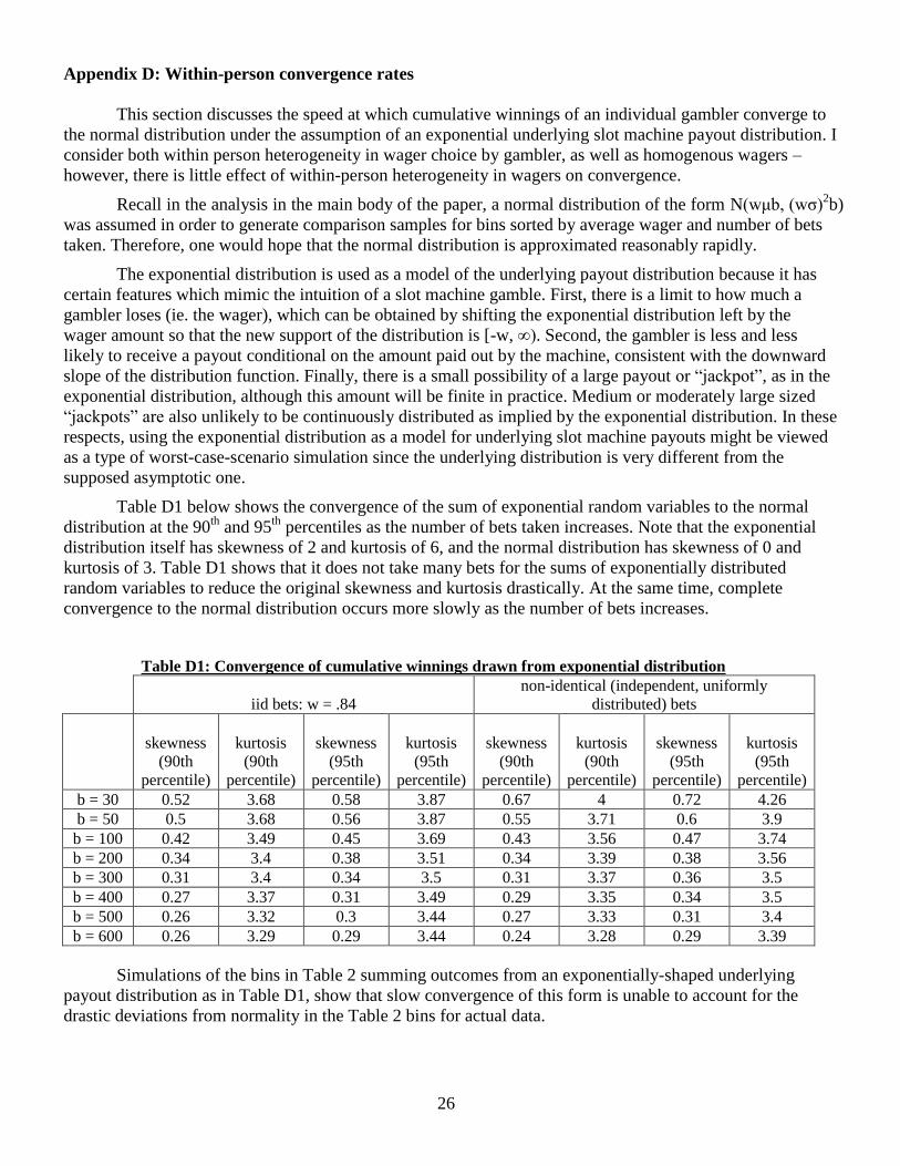
Appendix D: Within-person convergence rates

This section discusses the speed at which cumulative winnings of an individual gambler converge to

the normal distribution under the assumption of an exponential underlying slot machine payout distribution. I

consider both within person heterogeneity in wager choice by gambler, as well as homogenous wagers –

however, there is little effect of within-person heterogeneity in wagers on convergence.

Recall in the analysis in the main body of the paper, a normal distribution of the form N(wμb, (wσ)2b)

was assumed in order to generate comparison samples for bins sorted by average wager and number of bets

taken. Therefore, one would hope that the normal distribution is approximated reasonably rapidly.

The exponential distribution is used as a model of the underlying payout distribution because it has

certain features which mimic the intuition of a slot machine gamble. First, there is a limit to how much a

gambler loses (ie. the wager), which can be obtained by shifting the exponential distribution left by the

wager amount so that the new support of the distribution is [-w, ∞). Second, the gambler is less and less

likely to receive a payout conditional on the amount paid out by the machine, consistent with the downward

slope of the distribution function. Finally, there is a small possibility of a large payout or “jackpot”, as in the

exponential distribution, although this amount will be finite in practice. Medium or moderately large sized

“jackpots” are also unlikely to be continuously distributed as implied by the exponential distribution. In these

respects, using the exponential distribution as a model for underlying slot machine payouts might be viewed

as a type of worst-case-scenario simulation since the underlying distribution is very different from the

supposed asymptotic one.

Table D1 below shows the convergence of the sum of exponential random variables to the normal

distribution at the 90th

and 95th

percentiles as the number of bets taken increases. Note that the exponential

distribution itself has skewness of 2 and kurtosis of 6, and the normal distribution has skewness of 0 and

kurtosis of 3. Table D1 shows that it does not take many bets for the sums of exponentially distributed

random variables to reduce the original skewness and kurtosis drastically. At the same time, complete

convergence to the normal distribution occurs more slowly as the number of bets increases.

Table D1: Convergence of cumulative winnings drawn from exponential distribution

iid bets: w = .84

non-identical (independent, uniformly

distributed) bets

skewness

(90th

percentile)

kurtosis

(90th

percentile)

skewness

(95th

percentile)

kurtosis

(95th

percentile)

skewness

(90th

percentile)

kurtosis

(90th

percentile)

skewness

(95th

percentile)

kurtosis

(95th

percentile)

b = 30 0.52 3.68 0.58 3.87 0.67 4 0.72 4.26

b = 50 0.5 3.68 0.56 3.87 0.55 3.71 0.6 3.9

b = 100 0.42 3.49 0.45 3.69 0.43 3.56 0.47 3.74

b = 200 0.34 3.4 0.38 3.51 0.34 3.39 0.38 3.56

b = 300 0.31 3.4 0.34 3.5 0.31 3.37 0.36 3.5

b = 400 0.27 3.37 0.31 3.49 0.29 3.35 0.34 3.5

b = 500 0.26 3.32 0.3 3.44 0.27 3.33 0.31 3.4

b = 600 0.26 3.29 0.29 3.44 0.24 3.28 0.29 3.39

Simulations of the bins in Table 2 summing outcomes from an exponentially-shaped underlying

payout distribution as in Table D1, show that slow convergence of this form is unable to account for the

drastic deviations from normality in the Table 2 bins for actual data.