Embed Size (px)
Citation preview

Slow Invariant Manifolds
for Reactive-Diffusive Systems
Joshua D. MengersJoseph M. Powers
Department of Aerospace and Mechanical Engineering
University of Notre Dame
7th International Congress on Industrial and Applied Mathematics
Vancouver, British Columbia, CanadaJuly 21, 2011
J. Mengers Notre Dame SIM Reactive-Diffusive July 21, 2011 1 / 26

Outline
1 Motivation and Background
2 Model
3 ResultsOxygen DissociationZel’dovich Mechanism
4 Conclusions
J. Mengers Notre Dame SIM Reactive-Diffusive July 21, 2011 2 / 26
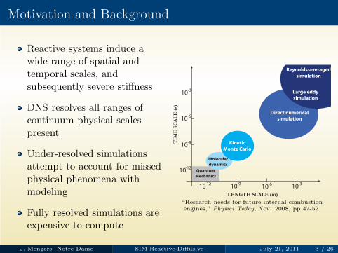
Motivation and Background
Reactive systems induce awide range of spatial andtemporal scales, andsubsequently severe stiffness
DNS resolves all ranges ofcontinuum physical scalespresent
Under-resolved simulationsattempt to account for missedphysical phenomena withmodeling
Fully resolved simulations areexpensive to compute
Direct numerical
simulation
Large eddy
simulation
Reynolds-averaged
simulation
Molecular
dynamics
Quantum
Mechanics
10-12
10-12
10-9
10-6
10-3
10-9
10-6
10-3
LENGTH SCALE (m)
TIM
E S
CA
LE
(s)
Kinetic
Monte Carlo
“Research needs for future internal combustionengines,” Physics Today, Nov. 2008, pp 47-52.
J. Mengers Notre Dame SIM Reactive-Diffusive July 21, 2011 3 / 26

Motivation and Background
Manifold methods providepotential savings
Most methods are for spatiallyhomogeneous systems
We employ the slow invariantmanifold (SIM) model ofAl-Khateeb, et al.(2009, Journal of Chemical Physics)
SIM
z3 Fast
Slow
Fast
Slow
z1
z2
We adjust for the dynamics ofdiffusion in the presence ofweak spatial heterogeneity
This is valid when diffusion isfast relative to reaction, i.e.thin regions of flames
J. Mengers Notre Dame SIM Reactive-Diffusive July 21, 2011 4 / 26
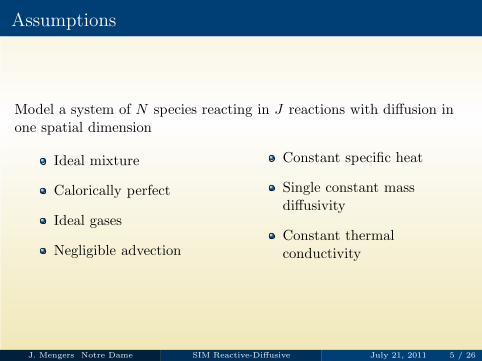
Assumptions
Model a system of N species reacting in J reactions with diffusion inone spatial dimension
Ideal mixture
Calorically perfect
Ideal gases
Negligible advection
Constant specific heat
Single constant massdiffusivity
Constant thermalconductivity
J. Mengers Notre Dame SIM Reactive-Diffusive July 21, 2011 5 / 26

Balance Laws
Evolution of species and energy
ρ∂Yi
∂t+
∂jmi
∂x= Miωi(Yn, T ), for i, n ∈ [1, N ]
ρ∂h
∂t+
∂jq
∂x= 0
Boundary conditions
∂Yi
∂x
∣∣∣∣x=0
=∂Yi
∂x
∣∣∣∣x=ℓ
= 0, for i ∈ [1, N ]
∂T
∂x
∣∣∣∣x=0
=∂T
∂x
∣∣∣∣x=ℓ
= 0
Initial conditions
Yi(x, t = 0) = Yi(x), for i ∈ [1, N ]
T (x, t = 0) = T (x)
J. Mengers Notre Dame SIM Reactive-Diffusive July 21, 2011 6 / 26

Constitutive Equations
Simple diffusive flux terms
jmi = −ρD
∂Yi
∂x, for i ∈ [1, N ]
jq = −k∂T
∂x+
N∑
i=1
hfi jm
i
Caloric equation of state
h =
N∑
i=1
Yi
(
cPi(T − T o) + hfi
)
Ideal gas equation of state
P =ρRT
∑Ni=1
Mi
Yi
J. Mengers Notre Dame SIM Reactive-Diffusive July 21, 2011 7 / 26
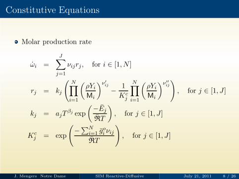
Constitutive Equations
Molar production rate
ωi =
J∑
j=1
νijrj , for i ∈ [1, N ]
rj = kj
(N∏
i=1
(ρYi
Mi
)ν′
ij
−1
Kcj
N∏
i=1
(ρYi
Mi
)ν′′
ij
)
, for j ∈ [1, J ]
kj = ajTβj exp
(−Ej
RT
)
, for j ∈ [1, J ]
Kcj = exp
(
−∑N
i=1 goi νij
RT
)
, for j ∈ [1, J ]
J. Mengers Notre Dame SIM Reactive-Diffusive July 21, 2011 8 / 26
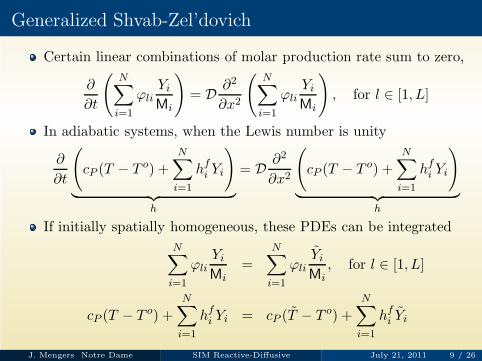
Generalized Shvab-Zel’dovich
Certain linear combinations of molar production rate sum to zero,
∂
∂t
(N∑
i=1
ϕli
Yi
Mi
)
= D∂2
∂x2
(N∑
i=1
ϕli
Yi
Mi
)
, for l ∈ [1, L]
In adiabatic systems, when the Lewis number is unity
∂
∂t
(
cP (T − T o) +
N∑
i=1
hfi Yi
)
︸ ︷︷ ︸
h
= D∂2
∂x2
(
cP (T − T o) +
N∑
i=1
hfi Yi
)
︸ ︷︷ ︸
h
If initially spatially homogeneous, these PDEs can be integrated
N∑
i=1
ϕli
Yi
Mi
=
N∑
i=1
ϕli
Yi
Mi
, for l ∈ [1, L]
cP (T − T o) +
N∑
i=1
hfi Yi = cP (T − T o) +
N∑
i=1
hfi Yi
J. Mengers Notre Dame SIM Reactive-Diffusive July 21, 2011 9 / 26

Reduced Variables
Transform to specific mole concentrations
zi =Yi
Mi
, for i ∈ [1, N − L]
Evolution of remaining L species and temperature are coupled tothese reduced variables by the algebraic constraints
∂zi
∂t=
ω(zn, T )
ρ+ D
∂2zi
∂x2, for i, n ∈ [1, N − L]
T =
T , if isothermal
h −∑N
i=1 zi(zn)hfi
∑Ni=1 zi(zn)cPi
+ T o, if adiabatic
J. Mengers Notre Dame SIM Reactive-Diffusive July 21, 2011 10 / 26
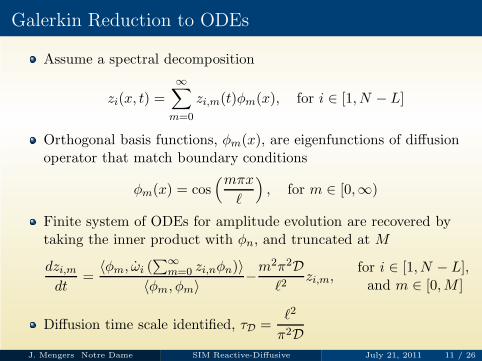
Galerkin Reduction to ODEs
Assume a spectral decomposition
zi(x, t) =
∞∑
m=0
zi,m(t)φm(x), for i ∈ [1, N − L]
Orthogonal basis functions, φm(x), are eigenfunctions of diffusionoperator that match boundary conditions
φm(x) = cos(mπx
ℓ
)
, for m ∈ [0,∞)
Finite system of ODEs for amplitude evolution are recovered bytaking the inner product with φn, and truncated at M
dzi,m
dt=
〈φm, ωi (∑
∞
m=0 zi,nφn)〉
〈φm, φm〉−
m2π2D
ℓ2zi,m,
for i ∈ [1, N − L],and m ∈ [0,M ]
Diffusion time scale identified, τD =ℓ2
π2D
J. Mengers Notre Dame SIM Reactive-Diffusive July 21, 2011 11 / 26

Oxygen Dissociation
O + O + M ⇌ O2 + M
N = 2 species
J = 1 reactions
L = 1 constraints
N − L = 1 reduced variablesz = zO
Isochoric,ρ = 1.6 × 10⁻⁴ g/cm3
Isothermal, T = 5000 K
Partial differential equation governing evolution
∂z
∂t= 249.84130 − 74734.78 z2 − 172406.48 z3 + D
∂2z
∂x2
J. Mengers Notre Dame SIM Reactive-Diffusive July 21, 2011 12 / 26

Oxygen Dissociation
O + O + M ⇌ O2 + M
N = 2 species
J = 1 reactions
L = 1 constraints
N − L = 1 reduced variablesz = zO
Isochoric,ρ = 1.6 × 10⁻⁴ g/cm3
Isothermal, T = 5000 K
Spatially homogeneous evolution equation
dz0
dt= 249.84130 − 74734.78 z2
0 − 172406.48 z30
-0.4 -0.3 -0.2 -0.1 0.1
-1500
-1000
-500
500
z(m
ol/g
)
ω (mol/g/s)
R1 R2 R3
J. Mengers Notre Dame SIM Reactive-Diffusive July 21, 2011 12 / 26

Diffusion-Correction – Galerkin Projection
One spatial mode (M = 1) evolution equation
dz0
dt= 249.84130 − 74734.78
(
z20 +
z21
2
)
− 172406.48
(
z30 +
3z0z21
2
)
dz1
dt= −74734.78 (2z0z1) − 172406.48
(
3z20z1 +
3z31
4
)
−π2D
ℓ2z1
Spatially homogeneousevolution when z1 = 0
Spatially homogeneousequilibria retained
Eigenvalues about theseequilibria are modified
λ1 = λ0 −π2D
ℓ2
0.2 0.5 1 2
10-5
10-4
0.001
ℓ (mm)
τ (s)
λ0 R3λ0 R2
λ1 R3λ1 R2
J. Mengers Notre Dame SIM Reactive-Diffusive July 21, 2011 13 / 26

Bifurcation
Change in sign of modified eigenvalue, λ1 = λ0 −π2D
ℓ2, identifies a
critical length where SIM origin changes character
Bifurcation occurs at R2
equilibrium
π2D
ℓ2= λ0 = 7321.5 s−1
ℓ = 1.04 mm
Diffusion-corrected SIM originshifts to bifurcated branches
1.035 1.040 1.045 1.050 1.055 1.060 1.065- 0.03
- 0.02
- 0.01
0.00
0.01
0.02
0.03
ℓ (mm)
z 1(m
ol/g
)
Locus of roots near R2
Bold branches are saddles; dashed branch is source
J. Mengers Notre Dame SIM Reactive-Diffusive July 21, 2011 14 / 26

Poincare Sphere
Map variables into a space where infinity is on the unit circle
η0 =αz0
√
1 + α2z20 + α2z2
1
η1 =αz1
√
1 + α2z20 + α2z2
1
ℓ = 0.334 mm
-1.0 -0.5 0.0 0.5 1.0
0.0
0.2
0.4
0.6
0.8
1.0
SIM
η0
η1
J. Mengers Notre Dame SIM Reactive-Diffusive July 21, 2011 15 / 26
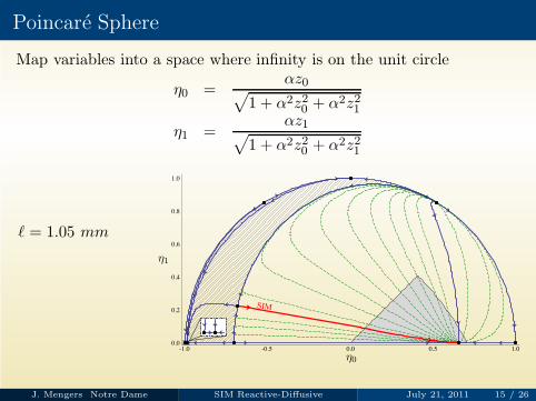
Poincare Sphere
Map variables into a space where infinity is on the unit circle
η0 =αz0
√
1 + α2z20 + α2z2
1
η1 =αz1
√
1 + α2z20 + α2z2
1
ℓ = 1.05 mm
-1.0 -0.5 0.0 0.5 1.00.0
0.2
0.4
0.6
0.8
1.0
SIM
η0
η1
J. Mengers Notre Dame SIM Reactive-Diffusive July 21, 2011 15 / 26
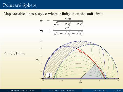
Poincare Sphere
Map variables into a space where infinity is on the unit circle
η0 =αz0
√
1 + α2z20 + α2z2
1
η1 =αz1
√
1 + α2z20 + α2z2
1
ℓ = 3.34 mm
-1.0 -0.5 0.0 0.5 1.0
0.0
0.2
0.4
0.6
0.8
1.0
SIM
η0
η1
J. Mengers Notre Dame SIM Reactive-Diffusive July 21, 2011 15 / 26
Zel’dovich Mechanism – Isothermal
N + NO ⇌ N2 + O
N + O2 ⇌ NO + O
N = 5 species
J = 2 reactions
L = 3 constraints
N − L = 2 reduced variablesz1 = zNO, z2 = zN
Isochoric, ρ = 1.2002 g/cm3
Isothermal, T = 4000 K
Bimolecular, isobaric,P = 1.6629 × 10⁶ dyne/cm2 =1.64 atm
Partial differential equation governing evolution
∂z1
∂t= 250−9.97×10⁴z1+1.16×10⁷z2−3.22×10⁹z1z2+6.99×10⁸z2
2 + D∂2z1
∂x2
∂z2
∂t= 250+8.47×10⁴z1−1.17×10⁷z2−1.84×10⁹z1z2−6.98×10⁸z2
2 + D∂2z2
∂x2
J. Mengers Notre Dame SIM Reactive-Diffusive July 21, 2011 16 / 26

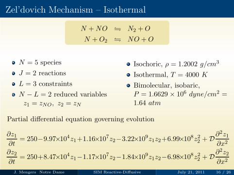
Zel’dovich Mechanism – Isothermal
N + NO ⇌ N2 + O
N + O2 ⇌ NO + O
N = 5 species
J = 2 reactions
L = 3 constraints
N − L = 2 reduced variablesz1 = zNO, z2 = zN
Isochoric, ρ = 1.2002 g/cm3
Isothermal, T = 4000 K
Bimolecular, isobaric,P = 1.6629 × 10⁶ dyne/cm2 =1.64 atm
Spatially homogeneous evolution equations – second order polynomials.
dz1,0
dt= 250−9.97×10⁴z1,0+1.16×10⁷z2,0−3.22×10⁹z1,0z2,0+6.99×10⁸z2
2,0
dz2,0
dt= 250+8.47×10⁴z1,0−1.17×10⁷z2,0−1.84×10⁹z1,0z2,0−6.98×10⁸z2
2,0
J. Mengers Notre Dame SIM Reactive-Diffusive July 21, 2011 16 / 26
Spatially Homogeneous Isothermal Phase Space
Identify equilibria
Characterize equilibriaby eigenvalues of theirJacobian matrix
Classify time scales asfast and slow
Identify SIM as aheteroclinic orbit fromsaddle to sink
SIM
−0.01 0 0.01 0.02
−0.02
−0.01
0
0.01
0.02
z1 (mol/g)
z 2(m
ol/g
)
R3R2
R1
I1
J. Mengers Notre Dame SIM Reactive-Diffusive July 21, 2011 17 / 26
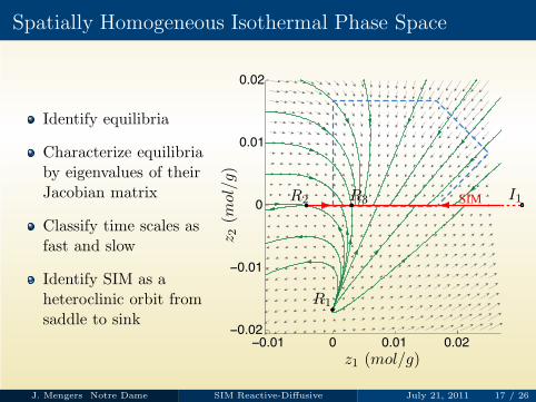

Spatially Homogeneous Isothermal Phase Space
Identify equilibria
Characterize equilibriaby eigenvalues of theirJacobian matrix
Classify time scales asfast and slow
Identify SIM as aheteroclinic orbit fromsaddle to sink
−4 −3 −2 −1 0 1 2 3
−3
−2
−1
0
1
2
3
x 10−5
SIM
x 10−3
z1 (mol/g)
z 2(m
ol/g
)
R3
R2
J. Mengers Notre Dame SIM Reactive-Diffusive July 21, 2011 17 / 26

Diffusion-Correction – Galerkin Projection
First diffusion mode addsmodified time scale
Positive eigenvalue identifiescritical length scale
139.46 139.47 139.48 139.49 139.50
- 2
- 1
0
1
2
x 10−5 Locus of roots near R2
z 1,1
(mol
/g)
ℓ (µm)
10 20 50 100 200 500 1000
10-8
10-7
10-6
10-5
ℓ (µm)
τ (s)
λi,0 R3λi,0 R2
λi,1 R3λi,1 R2
Bifurcation occurs at thislength scale
Let us examine a length belowthis critical length scale,ℓ = 17 µm
J. Mengers Notre Dame SIM Reactive-Diffusive July 21, 2011 18 / 26
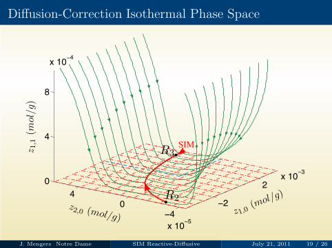
Diffusion-Correction Isothermal Phase Space
−2
2
x 10−3
−4
0
4
x 10−5
0
4
8
x 10−4
SIM
z1,0(mol/g
)z2,0 (mol/g)
z 1,1
(mol
/g)
R3
R2
J. Mengers Notre Dame SIM Reactive-Diffusive July 21, 2011 19 / 26

Diffusion-Correction Isothermal Evolution
10−10
10−8
10−6
10−4
10−20
10−15
10−10
10−5
1 , 0
2 , 0
1 , 1
2 , 1
t (s)
z i,m
(mol
/g)
zzzz 0
8.5
17
10−10
10−8
10−6
10−4
0
5
10
15
x 10−4
t (s)
z NO
(mol
/g)
x (µm)
Two additional fast time scales from diffusion
Spatially inhomogeneous amplitudes decay earlier than eitherreaction time scale
J. Mengers Notre Dame SIM Reactive-Diffusive July 21, 2011 20 / 26

Zel’dovich Mechanism – Adiabatic
N + NO ⇌ N2 + O
N + O2 ⇌ NO + O
N = 5 species
J = 2 reactions
L = 3 constraints
N − L = 2 reduced variablesz1 = zNO, z2 = zN
T = T (z1, z2)
Isobaric,P = 1.6629 × 10⁶ dyne/cm2
= 1.64 atm
Adiabatic,h = 9.0376 × 10⁻¹⁰ erg/gchosen to keep chemicalequilibrium at same point
Evolution equations highly nonlinear due to temperature-dependancein exponentials
J. Mengers Notre Dame SIM Reactive-Diffusive July 21, 2011 21 / 26
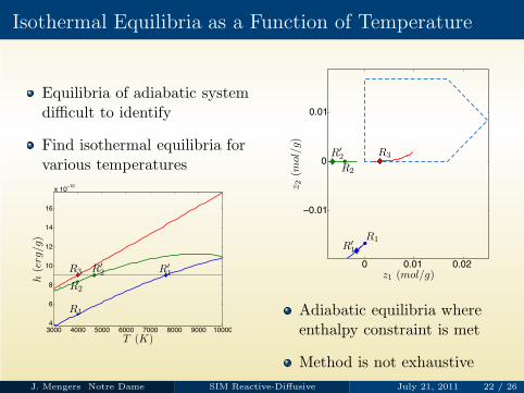
Isothermal Equilibria as a Function of Temperature
Equilibria of adiabatic systemdifficult to identify
Find isothermal equilibria forvarious temperatures
3000 4000 5000 6000 7000 8000 9000 10000
4
6
8
10
12
14
16
x 10−10
h(e
rg/g
)
T (K)
R3
R2
R1
R′
2 R′
10 0.01 0.02
−0.01
0
0.01
z1 (mol/g)
z 2(m
ol/g
)
R3
R2
R1
R′2
R′1
Adiabatic equilibria whereenthalpy constraint is met
Method is not exhaustive
J. Mengers Notre Dame SIM Reactive-Diffusive July 21, 2011 22 / 26
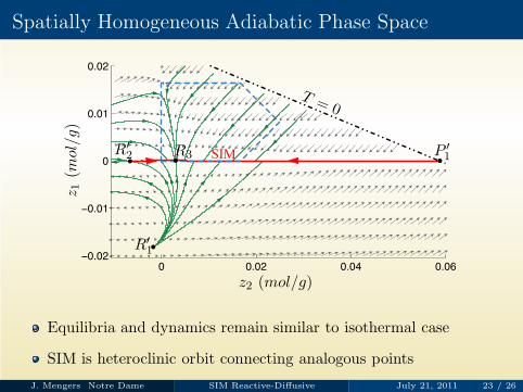
Spatially Homogeneous Adiabatic Phase Space
0 0.02 0.04 0.06
−0.02
−0.01
0
0.01
0.02
SIM
z 1(m
ol/g
)
z2 (mol/g)
R3R′2
R′
1
P ′
1
T = 0
Equilibria and dynamics remain similar to isothermal case
SIM is heteroclinic orbit connecting analogous points
J. Mengers Notre Dame SIM Reactive-Diffusive July 21, 2011 23 / 26

Spatially Homogeneous Adiabatic Phase Space
−6 −4 −2 0 2 4−8
−6
−4
−2
0
2
4x 10
−5
SIM
x 10−3
z 1(m
ol/g
)
z2 (mol/g)
R3
R′2
Equilibria and dynamics remain similar to isothermal case
SIM is heteroclinic orbit connecting analogous points
J. Mengers Notre Dame SIM Reactive-Diffusive July 21, 2011 23 / 26

Spatially Homogeneous Adiabatic Evolution
10−10
10−8
10−6
10−4
10−4
10−3
10−2
zNO
zN
zN2
zO
zO2
z(m
ol/g
)
t (s)10
−10
10−8
10−6
10−4
2000
2500
3000
3500
4000
T(K
)
t (s)
Species and temperature evolution exhibit fast and slow timescales, consistent with equilibrium eigenvalues
Adiabatic reactive-diffusive systems have yet to be analyzed
J. Mengers Notre Dame SIM Reactive-Diffusive July 21, 2011 24 / 26
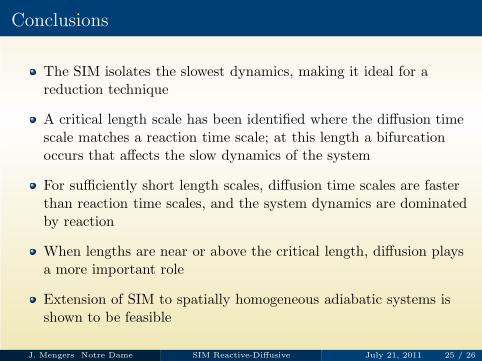
Conclusions
The SIM isolates the slowest dynamics, making it ideal for areduction technique
A critical length scale has been identified where the diffusion timescale matches a reaction time scale; at this length a bifurcationoccurs that affects the slow dynamics of the system
For sufficiently short length scales, diffusion time scales are fasterthan reaction time scales, and the system dynamics are dominatedby reaction
When lengths are near or above the critical length, diffusion playsa more important role
Extension of SIM to spatially homogeneous adiabatic systems isshown to be feasible
J. Mengers Notre Dame SIM Reactive-Diffusive July 21, 2011 25 / 26

Acknowledgments
Partial support provided by NSF Grant No. CBET-0650843,
Notre Dame ACMS Department Fellowship, and SIAM travel grant
J. Mengers Notre Dame SIM Reactive-Diffusive July 21, 2011 26 / 26