Embed Size (px)
Citation preview

Rochester Institute of Technology Rochester Institute of Technology
RIT Scholar Works RIT Scholar Works
Theses
1984
Small D.C. bipolar electromagnetic design: optimization and Small D.C. bipolar electromagnetic design: optimization and
analysis analysis
John J. Breen
Follow this and additional works at: https://scholarworks.rit.edu/theses
Recommended Citation Recommended Citation Breen, John J., "Small D.C. bipolar electromagnetic design: optimization and analysis" (1984). Thesis. Rochester Institute of Technology. Accessed from
This Thesis is brought to you for free and open access by RIT Scholar Works. It has been accepted for inclusion in Theses by an authorized administrator of RIT Scholar Works. For more information, please contact [email protected].
SMALL
D.C. BIPOLAR
ELECTROMAGNET
DESIGN
OPTIMIZATION AND ANALYSIS
by
John Joseph Breen
Submitted in Partial Fulfillment
of the
Requirements for the Degree
Master of Science
Supervised by Ray C. Johnson, Ph.D.
Department of Mechanical Engineering
Rochester Institute of Technology
Rochester, New York
1984
SMALL D.C. BIPOLAR ELECTROMAGNET DESIGN
OPTIMIZATION AND ANALYSIS
by
John J. Breen
Submitted
in
Partial Fulfillment
of the
Requirements for the Degree of
MASTER OF SCIENCE
in
Mechanical Engineering
Approved by:
Prof. Ray C. Johnson('l'hest's Advi'Sor)
Prof. [Illegible]
Prof. [Illegible] Gupta
Prof. P. Marletcar~Departmeht Head)
DEPARTMENT OF MECHANICAL ENGINEERING
COLLEGE OF ENGINEERING
ROCHESTER INSTITUTE OF TECHNOLOGY
ROCHESTER, NEW YORK
MAY, 1984

Gr-^^
I OQU'aJ *^J Q^aJ prefer to be contacted
each time a request for reproduction is made. I can be reached
at the following address. *-rl KbcQUiDS, ~L)Q.
Date : S/e/S^

ACKNOWLEDGEMENTS
I would like to take this opportunity to thank my
advisor for his help and guidance through this project. The
knowledge gained from his courses and its application to this
project is, without question, the most useful and important
segment of my graduate education. If all the curriculum
required for degree work could be as practical and meaningful
as the optimization techniques he presents, the worth of a
graduate engineer would rise considerably.
I would also like to thank my employer and fellow
workers for their support and understanding throughout this
effort. Their teamwork spirit has been appreciated. The B-H
testing was not a complete success, but it would not have
occurred at all without the help of the personnel and use of
equipment at the research labs.
Finally, and most important, I would like to thank my
wife and two sons for their support and understanding
throughout the graduate school period. Without their
patience, the efforts could not have been completed. It is
to them that I dedicate this work.
11

ABSTRACT
The design of electromagnets is an iterative process in
which the designer arrives at a solution to his design
problem through repeated design trials. This procedure can
be time consuming, and the resultant configuration may or may
not be the best one for the constraints imposed on it. In
addition, the designer must have a reasonable knowledge of
magnetics to carry out these design steps.
This paper presents the basic equations necessary for
designing and analyzing a horseshoe-shaped D.C. electro
magnet. With this base, two methods are developed to
optimize a design for maximum holding force, subject to
prespecified constraints. The first method is a graphical
approach. The advantage of this method is that it presents,
in a simple manner, the effects of changes in the design
constraints on the final solution. The disadvantage is that
the user must thoroughly understand the design equations to
use it.
The second method is part of a complete computer program
package, written in Basic for an Apple 11+ computer. This
package can be used by a designer with little or no knowledge
of magnetics, the equation system, or the program. It not
only designs the maximum holding force electromagnet for the
constraints imposed, but also analyzes existing designs for
iii
many of the characteristics and sensitivities needed to
insure a good production coil. The graphics capabilities of
the Apple microcomputer are used extensively for maximum
clarity.
Holding force experiments are also presented, which are
used to confirm the predicted results from the computer
simulations. Good correlation is demonstrated for the
configuration tested. Partial data is also presented for
determining the B-H curves of various densities of sintered
50/50 nickel iron material.
The combination of the program and paper is a useful
tool for an engineer faced with an electromagnet design
problem. It should result in a significant reduction in the
time required to arrive at an acceptable solution.
IV
TABLE OF CONTENTS
Page
ACKNOWLEDGMENTS ii
ABSTRACT iii
LIST OF FIGURES viii
NOMENCLATURE and VARIABLES ix
EQUATION SUMMARY xi
Chapter Title
I- INTRODUCTION 1
1.1 Background 1
1.2 Purpose of Project 2
II CONVENTIONAL METHOD OF COIL ANALYSIS .... 7
2.1 Introduction 7
2.2 Number of Turns 9
2.3 Other Geometrically Determined Values. . 11
2.4 Amp Turns 12
2.5 Magnetic Concepts and Units 14
2.6 D.C. Magnetization Curves 16
2.7 Fringing Effects at the Magnet Poles . . 18
2.8 Determination of Amp Turn Distribution . 18
2.9 Holding Force 21
2.10 Flux Leakage or Loss 21
2.11 Thermal Considerations 23
2.12 Other Items of Interest 30
2.13 Conclusions 31
III INITIAL INVESTIGATIONS AND FIRST
OPTIMIZATION METHOD 33
3.1 Introduction 33
3.2 Assumptions for the First Optimization
Method 35
3.3 First Optimization Method 37
3.4 An Example of the First Method 3 8
3.5 Conclusions 44
IV CURVE FITS 4 9
4.1 Introduction 4 9
4.2 Bare Wire Diameters 49
4.3 Ohms per Unit Length 51
4.4 Insulated Wire Diameters 52
4.5 Thermal Coefficients 53
4.6 B-H Curve Digitization 54
V SECOND OPTIMIZATION METHOD: PROGRAM OVERVIEW 55
5.1 Introduction 55
5.2 Program Structure and File Management. . 56
5.3 Memory Management 59
5.4 Shapefile 62
5.5 Final Note 63
v
Chapter Title Page
VI PAGE 1 PROGRAM MODULE 64
6.1 Module Purpose 64
6.2 Program Flow 64
6.3 Special Program Notes 67
VII PAGE 2-A PROGRAM MODULE 68
7.1 Introduction 68
7.2 Program Size Considerations 68
7.3 Other Functions 70
7.4 Special Programming Notes 71
VIII B-H ENTRY PROGRAM MODULE 73
8.1 Program Function and Flow 73
8.2 Basic Concept 75
8.3 Observations on the Method 76
8.4 Special Programming Notes 77
IX ANALYSIS PROGRAM MODULE 78
9.1 Program Function and Flow 78
9.2 Assumptions and Constants 79
9.3 Amp Turn Distribution Calculations ... 80
9.4 Special Programming Notes 86
X COIL DESIGN MODULE 87
10.1 Introduction 87
10.2 Optimization Problem Embedment 88
10.3 Notable Problems 93
10.4 Programming Notes 100
XI SAMPLE RUNS AND OBSERVATIONS 101
11.1 Introduction 101
11.2 Sample Runs 102
11.3 Observations and Conclusions 129
XII HOLDING FORCE EXPERIMENTS 141
12.1 Purpose of the Experiments 141
12.2 Description of Apparatus 143
12.3 Experimental Results and Calculations. . 146
12.4 Core Density Experimental Results. . . . 150
12.5 Solid Core Experimental Results 154
12.6 Observations and Conclusions 158
XIII B-H CURVE DETERMINATION EXPERIMENTS 163
13.1 Purpose of the Experiment 163
13.2 Description of Apparatus and Procedure . 163
13.3 Presentation of Data 164
13.4 Observations and Conclusions 167
XIV CONCLUSIONS AND RECOMMENDATIONS FOR FURTHER
STUDY 168
vi
Appendix
A
B
Title Page
H
References,
FIRST OPTIMIZATION METHOD 175
A.l Program Listing 176
PAGE 1 PROGRAM MODULE 177
B.l Program Listing 178
B.2 Program Length and XRef 183
PAGE 2-A PROGRAM MODULE 184
C.l Program Listing 185
C.2 Program Length and XRef 217
B-H PROGRAM MODULE 221
D.l Program Listing 222
D.2 Program Length and XRef 232
ANALYSIS PROGRAM MODULE 233
E.l Program Listing 234
E.2 Program Length and XRef 24 9
COIL DESIGN PROGRAM MODULE 253
F.l Program Listing 254
F.2 Program Length and XRef 282
WIRE DATA INFORMATION 287
G.l Comparison of Calc and Table Bare Dias. 288
G.2 Comparison of Calc and Table Ins Dias . 289
G.3 Comparison of Calc and Table Wires/sq-in 290
G.4 Comparison of Calc and Table Ohms/ft. . 291
G.5 Sample Page of Standard Wire Table. . . 292
INITIAL MAGNETIZATION CURVES FOR MATERIALS. 2 93
H.l Semi-Log Graph for Various Magnetic Mat 294
SAMPLE OF DISK CATALOG 295
1.1 Catalog Listing 296
ADDITIONAL COMPUTER TRIALS 297
J.l TEST-SQ-S-D3 w/COLD ROLLED STEEL CORE . 298
J. 2 TEST-SQ-S-D3 w/3% Si-STRIP CORE .... 302
J. 3 TEST-SQ-S-D5 optim w/3% Si-Strip CORE . 306
J. 4 TEST-SQ-S-D7 optim w/C.R. Steel CORE . . 310
314
Bibliography 315
vn

LIST OF FIGURES
Figure Title Page
1 Variable Locations 8
2 D.C. Magnetization Curve for 50/50 Ni-Fe ... 17
3 First Optimization Method for CA=0.09 39
4 First Optimization Method for CA=0.1225. ... 40
5 First Optimization Method for CA=0.160 .... 41
6 Comparison of Highest Force Designs 45
7 Program Flow 57
8 Memory Map 60
9 PAGE 1 Title and Prompt pages 65
10 B-H Entry Page 74
11 Flux vs mmf for Interpolation 82
12 Production Design-Design Requirements 105
13 Production Design-Actual Design 105
14 Production Design-Gap and Voltage Sensitivity. 106
15 Production Design-Analysis Output 107
16 TEST-SQ-S-D3-Design Requirements 109
17 TEST-SQ-S-D3-Optimum Design 109
18 TEST-SQ-S-D3-Gap and Voltage Sensitivity . . . 110
19 TEST-SQ-S-D3-Analysis Output Ill
2 0 TEST-RND-S-D4-Design Requirements 113
21 TEST-RND-S-D4-Optimum Design 113
22 TEST-RND-S-D4-Gap and Voltage Sensitivity. . . 114
23 TEST-RND-S-D4-Analysis Output 115
24 TEST-SQ-D-D-Design Requirements 117
25 TEST-SQ-D-D-Optimum Design 117
26 TEST-SQ-D-D-Gap and Voltage Sensitivity. . . . 118
27 TEST-SQ-D-D-Analysis Output 119
28 TEST-RND-D-D-Design Requirements 121
29 TEST-RND-D-D-Optimum Design 121
30 TEST-RND-D-D-Gap and Voltage Sensitivity . . . 122
31 TEST-RND-D-D-Analysis Output 123
32 CORE SHAPE TEST-Design Requirements 125
33 CORE SHAPE TEST-Optimum Design 125
34 CORE SHAPE TEST-Gap and Voltage Sensitivity. . 12 6
35 CORE SHAPE TEST-Analysis Output 127
36 Holding Force Experimental Apparatus 144
37 Holding Force for Airgaps 147
38 Holding Force for Density 151
39 Density vs Tonnage 152
40 Solid Core Holding Force w/Computer Overlay. . 156
41 Volts Increase for Fixed Gaps 159
42 Volts Increase for Fixed Force 161
43 B-H Curves-Uncorrected 166
Vlll

NOMENCLATURE
VARIABLE DESCRIPTION UNITS
A Area
AA intermediate constant (eqn 59)
AG Area of airGapAP Average turn Path length
B flux densityBA flux density in Air
BF Bobbin Flange thickness
BI flux density in Iron
C thermal CapacityCA Core Area
CD Core Depth
cgs centimeter/gram/second system
CI Coil current, I
CP Core Perimeter
CR Coil Resistance
CW Core Width
CI Clearance 1-bobbin to armature
C2 Clearance 2-bobbin to core
D Diameter
DO Depth Overall
dia of #n wire dia of gage #n
d( ) difference between 2 values
dTT/dt time differential of temperature
exp() e to the () power, exponent
F Force
Fa Flux-aim
Fl Flux-lower
FLUX magnetic FLUX
FT Force Total
Fu Flux-upper
FW Flange Width
G airGap length
h length of each pole
H magnetizing force
HA magnetizing force in Air
HI magnetizing force in Iron
ID Insulated wire Diameter
IN effective Insulated wire Number
II Intermediate value for CA and AG
12 Intermediate value for CA and AG
13 Intermediate value for AG
K heat dissipation capacity
KK intermediate constant
Kl force constant
k wire resistance constant, 10.372
L Length
LH inductance-Henries
sq-cm
cm
(kilo)gauss
(kilo)gauss
cm
(kilo)gauss
joules/degC
sq-cm
cm
amps
cm
ohms
cm
cm
cm
cm
degC/sec
oz
Maxwells
Maxwells
Maxwells
oz
Maxwells
cm
cm
inch
Oersteds
Oersteds
Oersteds
cm
watts/degC
ohms*CMil/ft
cm (ft in 47)
henries
IX

VARIABLE DESCRIPTION UNITS
LK heat dissipation coefficient
LO Length Overall
LOG natural LOGarithm
LW Length of WindingM Multiplier for coil type
m wire number
mmf magnetomotive force
mu magnetic material constant
NA Number of amp-turns in Air
NAa NA aim
NA1 NA lower
NAu NA upper
NC Number of turns Calculated
NI Number of amp-turns in Iron
NIa NI aim
Nil NI lower
NIu NI upper
NT Number of amp-turns Total
n wire gage number
OC Ohms per Centimeter for wire
01 Ohms per Inch for wire
P Power
P leakage Permeance (eqn 26 only)
PA Power per surface Area
PI constant=3. 14159
PL iron Path Length
Q optimization QuantityR Radius on core corners
R wire Resistance (eqn 47 only)
RE Resistance at Elevated temperature
REL RELuctance of magnetic material
RW Random Wind factor
SA Surface Area of coil
SI Standard International units
SM Surface area of coil
ST Steady state Temperature rise
TC thermal Time Constant
TT Temperature
t time
V Voltage
W Wall thickness
WD Wire Diameter
WG Wire Gage number
WO Width Overall
WP Winding Perimeter
WT WeighT of core
WW Winding Width
W2 Wires per cm**2
watt/degC/sq-in
cm
cm
. 4PI*amp-turns
gauss/oersted
amp-turns
amp-turns
amp-turns
amp-turns
turns
amp-turns
amp-turns
amp-turns
amp-turns
amp-turns
ohms/cm
ohms/in
watts
leakage/in
watts/sq-in
cm
1/oz
cm
ohms
ohms
sq-cm
(MKS)
sq-in
degC
sec
degC
sec
volts
cm
cm
cm
cm
pounds
cm
wires/sq-cm
x
EQUATION SUMMARY
No. Equation
1
2
3
4
5
5a
5b
6
7
8
9
10
11
12
13
14
15
16
17
18
19
19a
20
21
22
23
24
25
26
27
28
29
30
31
32
33
34
35
36
37
37a
38
39
40
41
42
43
NC = LW * WW * RW * W2
Efficiency = (PI * D * D / 4)/(D *D)
CP = 2 * (CD + CW + (PI - 4) * R)
+ 2 * PI * (W + WW / 2)AP
CA
CP
II *
II =
12 =
CD +
C2 +
LW +
2 *
R + 212 + 2 * II *
CD - 2 * R
CW - 2 * R
2 * (W + FW)
2 * (CW + W + FW)
CI + 2 * (CW + BF)
(LW + FW + W + CI +
12 R + PI * R R
DO
WO
LO
PL
CI = V / CR
CR = NC * (AP *OC)
NT = NC * V / NC / AP / OC
NT = V / AP / OC
B = mu* H
H = (0.4 * PI * (amp-turns)) / L
REL = L / mu / A
FLUX = B * A = mmf / REL
= mmf / REL
II * 12 + II * 13 + 2 *
13 = R + G / 2
NA + NI
HA = 0.4 * PI * NT / (G
0.4 * PI * NT / PL
BI * CA / AG
F = Kl * BA * BA * AG /FT = Kl * BA * BA * AG
INTERPOLAR FLUX LEAKAGE
P = (C * (dTT/dt) ) + (K
LOG ((P-K*TT)/P)=
C2 + 2 * (BF + CW) )
FLUX
AG =
NT =
BA =
HI =
BA =
12 13 + PI 13 13
2) (special case)
(special case)
/ (mu for air)
/ 2) *= (P * h
* TT)
-(K* t) /
NT h
(1 -
exp(-(K / C)
C
t)TT = (P / K)
ST = P / K
TC = C / K
K = SM * LK
P = PA * SM = CI * V
C = 180 * WT
WT = 0.015385 * AP * WW * RW * LW * PI / 4
WP = AP + PI * WW
SA = M * LW * WP
SM = SA / 2.54 / 2.54
t = -(C / K)* (LOG(P / K - 70) - LOG(P / K)
RE = CR * (ST + 20 + 234) / (254)
LH = NC * (FLUX IN WEBERS ) / CI
LH = NC * BA * AG / 100000 / CI
CW = CA / CD
FW = (DO - CD - 2 * W) / 2
xi

No. Equation Page
44 LW = V / CI / FW / RW / W2 / AP / OC 37
45 W2 = 1 / ID / ID 43
46 (dia of #n) = 0.324860745 * (0.890525717) **n 50
47R=k*L/A 51
48 OI = (8.64333333E-7) / WD / WD 51
49 OC - OI / 2.54 52
50 IN = LOG(ID / 0.324860745) / LOG ( 0 . 890525717 ) 52
51 IN = 0.967 * WG + 0.221 52
52 ID = 0.324860745 * 0.890525717 ** IN 53
53 LK = exp(PA)/(107.23*(PA+0.194)*(PA+0.194)+191.5) 54
54 FLUX = AG * HA 83
55 FLUX = (AG * 0 . 4 * PI / G ) * NA 83
56 LOG(HI) = LOG(NI) + LOG ( 0 . 4 * PI / PL) 83
57 (LOG(NIa) - LOG(NIl)) / (LOG(NIu) - LOG(NIl))=
(Fa - Fl) / (Fu -
Fl) = (NAa -
NAl) / (NAu - NA1 ) 84
58 NIa = NT - NAa 8 5
59 KK = LOG(NIa) + AA * NIa 85
59a AA = (LOG(NIu) -
LOG(NIl)) / (NAu -
NAl) 85
59b KK = AA * (NT - NAl) + LOG(NIl) 85
60 BA = SQRT(FT / Kl / AG) 130
61 NI = HI * PL / PI / 0.4 131
62 d(NT) = d(NA) 131
63 NT = NC * V / CR 131
64 d(NA) = d(V) * (NC / CR) 132
65 1000 * BA = HA = 0.4 * PI * NA / G / 2 132
66 G = 0.4 * PI * NA / BA / 2000 132
67 d(G) = d(NA) * 0.4 * PI / BA / 2000 132
68 d(BA) = d(NA) * (0.4 * PI / G / 2000) 160
69 d(G) = d(V) * (NC * 0.4 * PI / BA / CR / 2000) 162
70 A*WW**2+B*WW-CR/RW=0 173
7 0a A = PI * LW * W2 * OC 17 3
70b B = (CP + 2 * PI * W)* LW * W2 * OC 174
xn
CHAPTER I
INTRODUCTION
1.1 Background
The design of electromagnets is an iterative process in
which the designer arrives at a solution to his design
problem through repeated design trials. This procedure can
be time consuming, and the resultant design may, or may not,
be the best one for the constraints imposed on it. In
addition, the designer must have a reasonable knowledge of
magnetics to carry out these design steps.
In the product design process, several elements are
typically left until the end, with the hope that there is
enough room to fit them in. While it would be very nice to
know the final configuration for a design before the design
process begins, this is never the case. Initial layouts are
made, breadboards are built, and several elements are
generally left until the end for design. Typically these
include springs, electrical components, and electromagnets.
Part of the reason for this is that these must be engineered,
while the other elements are more creative, yet
straightforward. Perhaps it is because of the lengthy
calculations and understanding required that these elements
are put off until last. After all, it is difficult to design
a spring when the travel and force requirements are not
1
known. It is easier to define the physical requirements and
then calculate to see if a solution exists. The problem of
rearranging the simpler mechanical elements can then take
place to accommodate any required changes dictated by the
spring design.
An electromagnet is an order of magnitude more difficult
to design than a spring, and designers qualified in the art
of designing them are few. Some space is set aside for the
electromagnet, but the actual calculations are put off. When
it comes time to design the coil and the related parameters,
the general attitude can be one of wrapping some coils around
a nail to see what happens. If the nail supplies enough
holding force, the design is complete. If it does not,
either try a bigger nail or allow more room and try again.
1.2 Purpose of the Project
While this scenario is perhaps a little overstated, it
is not far from reality for most designers. In addition, the
electrical engineer is well-versed in how to calculate the
inductance or resistance, but not the holding force. The
mechanical engineer is no more knowledgable and often must
review an old text book to relearn some long forgotten
concepts.
The primary objective of this project is to prove, by
example, the hypothesis that for any set of design
constraints, there exists a maximum holding force

configuration. From the force equation which will be
developed, this will be intuitively clear. The reader will
realize that in the two extreme cases, zero force will exist.
At one limit, if the entire available space is filled with
core, no room will be left for coils. Then no force will be
developed. Similarly, if the entire volume is filled with
windings, a core will not be present. Again, no force will
be developed. Between these limits, varying amounts of
holding force can be calculated. The question is, for a
given set of constraints, how high is the potential force,
and what configuration of core and windings will produce it?
The second goal of this project is to develop an easy to
use algorithm and computer program for designing the
configuration of the maximum holding force, D.C. horseshoe
shaped electromagnet, which is subjected to a set of
prespecified constraints. The constraints must include
overall dimensions, selected electrical limits, and other
manufacturing considerations imposed as requirements. The
method of entry must be clear and concise, and the resulting
information sufficient to describe the coil in enough detail
to manufacture a sample. Device related attributes should
also be calculated.
The highest requirement, however, must be that the user
should not have to understand the magnetics involved or the
details of the program which performs the calculations. The
instructions required to use the developed program must be

minimal enough to encourage its use.
With these goals in mind, the equation system required
for analyzing a coil of the general size and shape being
considered will be developed. With this background, a
preliminary optimal design method will be developed,
programmed, and numerically applied to a set of design
constraints. While this first method will find the best
possible solution to the problem, it will not be user
friendly and method transparent.
To facilitate solution of the optimal design problem,
curve fitting techniques will be applied to the tabular data
normally used in the calculation process. A method of
digitization for magnetic B-H curves will also be developed,
which is simple to understand and easy to execute.
This base of information will then be used to develop a
design algorithm and a highly user friendly computer program
for use on an Apple 11+ computer equipped with a monitor and
disk drive. The program will make heavy use of the graphics
capabilities of that machine to meet the user friendly
requirements of the project. The completed package will not
only design the highest force coil for the given constraints,
but it can also analyze an existing coil for other
characteristics of interest. It will also show the
sensitivity of that design to variations in voltage supply
and airgap length.
In the event that incompatible specifications exist,

methods for overcoming those incompatibilities will be
suggested. In addition, the design which comes closest to
meeting the requirements will be shown, thereby helping the
designer decide which specifications should be changed to
result in an acceptable design. This eliminates the NO
DESIGNS FOUND problem of many commercial design packages for
other elements.
As a check on the theory, several experiments with a
commercially produced electromagnet will be conducted and
compared to the computer predictions. Using the overall
dimensions of the coil, the optimization method will be
applied to show how the original design can be improved. As
much as a fifty percent improvement will be calculated
using some dimensional changes suggested by the program. It
will be shown that the theory and actual practice do agree
quite well, and it will prove that the methods developed have
merit and a basis in fact.
Several new equations for determining airgap lengths and
other information about a given design will be developed and
used to explain the experimental data as well as the
sensitivity graphs which are part of the computer output.
Finally, an analysis will be given for the B-H
characteristics of sintered 50/50 nickel iron. While the
data is incomplete, the information presented can be of use
to some individuals. The information is not central to the
main theme of this project; and therefore, its completion is
not necessary. However, enough new information has been
collected to warrant inclusion in this report.
The automated design portion of this project is an
application of the P519RE optimization program developed by
Dr. Ray C. Johnson. The details of that program will not be
discussed in depth, but the problems peculiar to this project
will. For further information, Reference 1 should be
consulted.
Many of the equations, presented in what follows, were
developed specifically for this project. All equations are
numbered sequentially throughout the text, and an equation
number appears to the right of each. To the left of the
equations will appear a reference, if appropriate. Those
equations which are basic to magnetics are marked with a (B).
These are so common that any text or reference manual on the
subject will contain them. Any equation from a specific
reference will be noted. All remaining equations are the
original work of this author for the project being presented.
CHAPTER II
CONVENTIONAL METHOD OF COIL ANALYSIS
2.1 Introduction
Throughout this text, the example presented in this
chapter will be applied to each of the methods described.
This will provide a means of making direct comparisons and
reduce the need for recalculating some of the values which
need to be determined. Chapter II will present an analysis
of an existing design using conventional methods. It will
serve as a vehicle for reviewing the basic equations and
units involved. Several extra steps will be performed in an
attempt to present most of the equations needed later. These
equations will be required by each of the two methods of
optimal design developed for this design project.
Units of measure will be in the cgs system, with the
exception of holding force, which will be in ounces. The cgs
system was chosen over SI units because of the sizes of parts
being considered. Force is given in ounces since the
intended end user has not fully converted to the metric
system and, therefore, would specify force in ounces.
Figure 1, shows the locations for all the physical
dimension variables used throughout this paper. It is
intended as a guide only and is not to be considered an
actual assembly drawing. Many drafting rules, such as double
7

CI"bf"
LW A
i
G
~1~
i
d>-PL
A LO
i
DO
BF
W
(Ml Around)
iCyW
-WO-
^Mz\
C2
CW
-WW-
CD
-R(AIIAround)
*Section"A-A
VARIABLE LOCATIONS
-AP
FIGURE 1
dimensioning, have been violated to fit all the variables on
one drawing. For the first example, all of the variables
except LO, DO,WO, PL and AP will be considered as givens. In
addition, number 42 copper wire with a single build layer of
enamel, will be used. Unless stated otherwise, numerical
values shown apply to the project example only. They are not
to be taken as constants which apply to all coil
computations .
2 . 2 Number of Turns
Normally, the number of turns would be known, rather
than the physical dimensions for the wire space. To show the
equations which will be used later, however, the reverse
will apply. Several items are needed to calculate the number
of turns. The first is, wires per square centimeter, which
can be found in standard wire tables. An example of a
standard wire table page, showing single build enamel
insulation for wire gages 14 through 44, is presented in
Appendix G. Single build enamel insulation is the only type
considered for this project. All equations and concepts,
with the exception of those for determining insulated wire
diameter and wires per square inch, are valid for other
types. Single build enamel is normal for coils in the size
range being considered here. The value of wires per area for
#42 wire is given as 127,551 wires/sq-in or 19,770.4
wires/sq-cm. Using geometry and common units for each of the

10
the variables, the number of turns, NC, which will fit in a
winding area cross section, is given by equation one.
NC = LW * WW * RW * W2 (1)
In equation (1), NC is the number of turns, LW is the
length of the winding (0.825cm), WW is the winding width
(0.0609cm), W2 is the wires/sq-cm (19770.4), and RW (1) is
the random wind factor. For the numerical values given,
equation one gives the number of turns as NC=9 93.
Random wind factors are used to compensate for the
inability of a coil winder to fit the exact number of turns
per area specified in the tables on an actual sample. This
discrepancy may be due to factors such as crossed wires,
winder tension, paper separators and so forth. Since these
factors are very machine dependent, throughout this paper RW
will be set at a value of unity. The programs and equations
presented allow a value other than one to be entered. The
standard wire table values assume that the wires are touching
each other, and their centerlines are arranged to fall on the
corners of a square whose sides are equal to one wire
diameter. Therefore, the value for wires per square
centimeter is equal to the inverse of the square of the
outside diameter of the wire, including insulation. In
addition, the packing efficiency for any diameter D is 0.7854
as determined by equation (2).
( PI * D * D / 4 ) / (D * D) (2)
In this equation, the denominator is the area available
11
to each wire, expressed as the diameter squared. The
numerator is the cross sectional area of one wire. PI has
the value, 3.14159. This packing efficiency is achievable on
a properly set up, modern winding machine. As a comparison,
if the wires were set in a hexagonal packing arrangement, the
packing efficiency would equal 0.907- Therefore, there is
some allowance for error built into the standard wire table
values.
One assumption in the equation for the number of turns
is that all of the cross sectional area of the windings is
assumed to be used. In practice this is not the case, since
there must be an integral number of wire diameters in the
winding width. Any final design must account for this by
having the flange width, FW, greater than the winding width.
It is up to the designer to remember this fact when carrying
out a production design, especially when winding widths are
only a few wire diameters thick.
2.3 Other Geometrically Determined Values
Seven items can be calculated using simple geometry.
They are core perimeter, CP; average path length, AP; core
area, CA; overall depth, DO; overall width, WO; overall
length, LO; and iron path length, PL. The equations are
presented, without discussion, for later use.
CP = 2 * (CD + CW + (PI - 4) *R) (3)
AP = CP + 2 * PI * (W + WW / 2) (4)

12
CA = II * 12 + 2 * II * R + 2 * 12 * R + PI * R * R (5)
where: II = CD - 2 * R and 12 = CW - 2 * R (5a)
DO = CD + 2 * (W + FW) (6)
WO = C2 + 2 * (CW + W + FW) (7)
LO = LW + CI + 2 * (CW + BF) (8)
PL = 2 * (LW + FW + W + CI + C2 + 2 * (BF + CW) ) (9)
For values of CD=0. 295cm, CW=0.3cm, FW=0. 106cm, BF=0.15cm,
C1=0. 285cm, C2=0.07cm, R=0cm and W=0. 064cm the seven
calculated items are as follows.
CP = 1.19cm AP = 1.791cm CA = 0.0885sq-cm
DO = 0.635cm WO = 1.01cm LO = 2.01cm
PL = 4.5cm
The values for overall length, width and depth will be
used repeatedly in this paper when the optimal design methods
presented are used to find solutions which give higher
holding forces than the production design being discussed
now.
2 . 4 Amp Turns
The function of an electromagnet is to convert
electrical energy into a magnetic field which can be used to
perform some mechanical work. Before any calculations for
the magnetics can be carried out, the values which determine
the magnetomotive force must be known. This force is
proportional to the current in the coil, CI in amps, times
the number of turns, NC. It is, therefore, necessary to
13
calculate CI, using the fundamental electrical identity of
equation (10).
(B) CI = V / CR (10)
The coil resistance, CR, is found using equation (11),
where the resistance of an average turn of wire is multiplied
by the total number of turns.
CR = NC * (AP *OC) (11)
Turning to the wire tables, the ohms per centimeter, OC,
is found to be 0.0544 ohms/cm for #42 wire, which is
equivalent to 1.659 ohms/ ft. Thus, for the values already
given, the total coil resistance, CR is equal to 9 6.8 ohms.
For the three volt sample being considered, this results in a
current requirement of 0.031 amps. Multiplying this current
by the number of turns, yields a total of 30.8 amp-turns.
While these equations, which lead to total amp-turns,
NT, are correct, some manipulating of them will result in a
more compact form for later work. Combining equations (10)
and (11) and multiplying by NC turns gives equation (12).
NT = NC * V / NC / AP / OC (12)
Cancelling out the common NC term leaves the final form
shown by equation (13).
NT = V / AP / OC (13)
This shows a very important fact about total amp-turns.
The value is dependent on the voltage, wire size and average
(or mean) turn path length only- Number of turns will
determine the coil resistance, but has no bearing on the
14
total number of amp-turns in the system. Thus, once the
dimensions which determine Section A-A in Figure 1 have been
specified, the electrical resistance and current will be
(inversely) proportional to the winding length, LW.
2.5 Magnetic Concepts and Units
At this point, all of the non-magnetic equations have
been presented, which are required for determining the
characteristics of the example being considered. Before
examining the remainder of the problem, some concepts and
terms regarding magnetics should be reviewed. Only units in
the cgs system of measurements will be shown, with little
more than a brief explanation of the concepts. It is assumed
that the reader has already been exposed to the basic
equations relating to magnetics, and needs only a quick
review.
When an electric current passes through a conductor, it
sets up a series of closed loop paths of magnetic flux lines
about it, which follow the right hand rule. These lines are
measured in Maxwells. The density of that flux is
represented by the letter B and its units are Maxwells per
square centimeter or Gauss. This flux density is directly
related to the magnetizing force, H.
(B) B = mu* H (14)
The (constant) mu is a characteristic of the material
called its permeability. Magnetizing force, H, is directly
15
proportional to the magnetomotive force (mmf) mentioned
earlier.
(B) H=(0.4*PI*(amp-turns)) / L (15)
In equation (15), L is the length of the material
through which the flux must pass and the numerator is the
mmf. Units of mmf are Gilberts and of H are Oersteds.
An additional concept, which is often presented, is that
of the reluctance of the material. This is a measure of a
materials'
resistance to pass flux.
(B) REL = L / mu / A (16)
Variable A is the cross sectional area of the material.
Combining (14), (15), and (16) yields:
(B) FLUX = B * A = mmf / REL (17)
(B) FLUX = mmf / REL (18)
When trying to learn these relationships, it can be very
helpful to draw an analogy between the magnetic equation
system and an electrical one. Thus, the mmf can be
considered analogous to the electromotive force, volts; flux
to current; reluctance to resistance; flux density to current
density and permeability to conductivity. Carrying the
analogy one step further, when several reluctances are
connected in series, they can be added together to produce an
equivalent reluctance. Finally, magnetic flux, like
electrical current, must be conserved. This is analogous to
the Kirchoff law for current. Therefore, the sum of the flux
entering a node must equal the sum of the flux leaving that
16
node.
Unfortunately, the total electrical analogy is good for
conceptualizing the magnetic properties only. For air, the
value of mu is constant. In the cgs system, that constant is
conveniently equal to 1. Air, however, is not a good flux
conductor, and therefore, a high permeability material like
iron is required to produce a useful magnetic circuit. This
is where the problem with the concept and practical
calculations comes in.
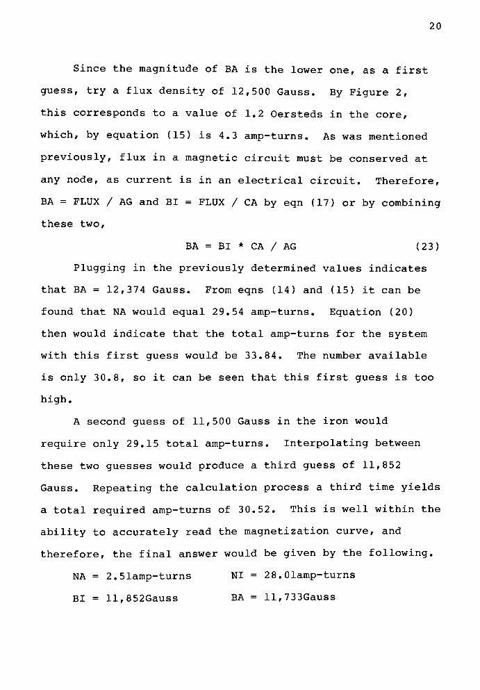
2.6 D.C. Magnetization Curves
Figure 2 shows a D.C. magnetization curve for solid
50/50 Nickel Iron. This is a graphical representation of
the initial relationship between B and H for a virgin sample
of that material. As can be seen, the value of B is no
longer related to the magnetizing force, H, by a constant mu,
but rather mu is a function of H. For the bipolar
electromagnet being studied, the total mmf must still be
divided between the metal path and the two airgaps as the
analogy to the electrical circuit suggests, but the
reluctance of the metal is dependent on the applied mmf. It
is this fact that makes a mathematical determination of the
mmf distribution very difficult, and is the reason a
graphical or an iterative approach is used to solve a
magnetic problem. Additional material curves are presented
in Appendix H for reference.

17
QIjJI-
(/)
CC
Ixl
oI
I
UJ
o
if
<N
\-
UJ
zo
<
CM
UJ
CC
OO^D'srCMO 00 (C * w
s3ssnv90iiJg_N0iiDnaN| oisniuin]
18
2.7 Fringing Effects at the Magnet Poles
With this fleeting description of the magnetic concepts,
the example problem can now be completed. Before continuing,
however, it is necessary to introduce one more concept
called fringing. When the flux is in a high permeability
material like the metal core of an electromagnet, it is
reasonably well confined within that material. When the air
is entered, however, the flux has a tendency to spread out
slightly, thereby increasing the area over which it is
spread. An approximation of this increased area can be made
by adding a band equal in width to one half of the airgap
around the perimeter of the core area (Ref 2). Thus the
equation for the area of the airgap, AG, is given by equation
(19).
AG = II * 12 + 2 * II * 13 + 2 * 12 * 13 + PI * 13 * 13 (19)
where 13 = R + G / 2 (19a)
Variable G is the length of one airgap. If G is set to
0.0015cm, then AG is equal to 0.0894sq-cm, for the example
being considered.
2.8 Determination of Amp Turn Distribution
The next step is to determine the number of amp turns
which are in the airgap, NA, and the number which are in the
iron, NI. The two are related by equation (20).
(B) NT = NA + NI (20)
19
Since the relative amounts in each is unknown, an iterative
approach must be used. To avoid a completely random starting
point, a first guess can be arrived at by making two extreme
assumptions. The first would be to assume that all the mmf
is in the air. The second, that all the mmf is used in the
iron. Either assumption will result in flux densities which
are too high. Therefore, a value slightly lower than the
smaller of the two can be used as a first trial.
If it is first assumed that all the mmf is in the air
then the flux density in the air, BA, by equations (14) and
(15), would be that shown by equation (21).
BA = HA = 0.4 * PI * NT / (G * 2) (21)
In this case, HA stands for the magnetizing force, H, in the
air. Since mu for air is unity in the cgs system, BA is
equal to HA by equation (14). The gap, G, is multiplied by 2
because there are a total of 2 airgaps in the system whose
combined length is twice G. Plugging in the appropriate
values results in a flux density in the air of BA = 12,901
Gauss, for the example.
If it is now assumed that all the mmf is in the core,
then the magnetizing force in the iron, HI, can be
calculated.
HI = 0.4 * PI * NT / PL (22)
For the values given, HI = 8.6 Oersteds. Referring to Figure
2, this would correspond to a value of slightly more than
14,000 Gauss for BI .
20
Since the magnitude of BA is the lower one, as a first
guess, try a flux density of 12,500 Gauss. By Figure 2,
this corresponds to a value of 1.2 Oersteds in the core,
which, by equation (15) is 4.3 amp-turns. As was mentioned
previously, flux in a magnetic circuit must be conserved at
any node, as current is in an electrical circuit. Therefore,
BA = FLUX / AG and BI = FLUX / CA by eqn (17) or by combining
these two,
BA = BI * CA / AG (23)
Plugging in the previously determined values indicates
that BA = 12,374 Gauss. From eqns (14) and (15) it can be
found that NA would equal 29.54 amp-turns. Equation (20)
then would indicate that the total amp-turns for the system
with this first guess would be 33.84. The number available
is only 30.8, so it can be seen that this first guess is too
high.
A second guess of 11,500 Gauss in the iron would
require only 2 9.15 total amp-turns. Interpolating between
these two guesses would produce a third guess of 11,852
Gauss. Repeating the calculation process a third time yields
a total required amp-turns of 3 0.52. This is well within the
ability to accurately read the magnetization curve, and
therefore, the final answer would be given by the following.
NA = 2.51amp-turns NI = 2 8 .
Olamp-turns
BI = ll,852Gauss BA = ll,733Gauss
21
2.9 Holding Force
Now, to calculate the primary item of interest. The
equation for holding force per airgap is given as by equation
(24).
(B) F = Kl * BA * BA * AG / 2 / (mu for air) (24)
For the example being considered, mu is equal to 1, and
there are two airgaps. Therefore, the total force will be
twice that specified for each airgap in equation (24). Kl is
a constant which is dependent on the units used. Since this
project is mixing the cgs units with force in ounces, the
value of Kl becomes 2.8696831. Combining these facts with
equation (24) produces a total force, FT, for a bipolar
electromagnet given by equation (25).
FT = Kl * BA * BA * AG (25)
Plugging the appropriate values of BA in kilogausses and
AG in sq-cm into the equation gives
FT = 35.32 ounces
for the example being considered.
2.10 Flux Leakage or Loss
This answer is not entirely correct. In addition to
fringing effects which have been accounted for, there are
losses of flux through various leakage paths. One set of
these paths is directly between the two poles of the magnet.
The leakage here is zero at the base (yoke) of the core and
increases linearly along the length of the poles.
22
Integrating along the length reveals that the total leakage
between the two poles is given as by equation (26),(Ref 3).
(R3) INTERPOLAR FLUX LEAKAGE =(P*h/2)*NT*h (26)
Here, P is the direct leakage permeance between the pole
cores per inch of axial length and h is the total length of
each pole. In addition to this leakage between the poles,
there are a complex set of leakage paths between the armature
and the length of the poles which protrude beyond the bobbin.
Due to the dependence of these leakages on geometry of the
parts and other factors, the calculation of the total flux
leakage becomes a non trivial task. The reader is referred
to articles 46, 54 and 55 of the text by Roters for a more
detailed explanation. For the scope of this project, the
flux loss will be assumed to be equal to a constant 20% for
any design. This leaves 80% of the calculated flux for
doing useful work at the airgap.
It must be remembered that when calculating the amount of
flux the core can carry, that the base (yoke) is passing all
of the flux calculated. It will saturate first, and is,
therefore, the limiting factor. The 80% factor must apply
only when calculating force, and since the force is
proportional to the square of the flux density, only 64% of
the calculated, no leakage force will be available.
Applying the 64% factor to the previously calculated FT
leaves a total expected force for the example of:
FT = 22.6 ounces
23
It can be seen that these losses are a significant factor,
and cannot be ignored.
One possible improvement to the design suggested by
this discussion would be to have tapered poles, with a large
cross section at the base to carry the higher level of flux.
This would result in a tapered bobbin, which would be
difficult to wind in actual practice, and also cause other
manufacturing problems. Since the aim of this project is to
provide a simple means of designing practical electromagnets,
the task of investigating this possibility will be left to
some other inquisitive mind. Many of the equations presented
here and in other texts would not apply in this case and a
return to the fundamental equations and concepts would be
required.
2.11 Thermal Considerations
Now that the coil has been analyzed for holding force
and other parameters, it would be easy to conclude that the
job is done. Unfortunately, factors other than holding force
and physical dimensions can make an otherwise acceptable
design incompatible with its intended function.
Frequently, heating is the predominant problem with an
electromagnet design. A more detailed explanation of the
discussion which follows may be found in Reference 4. Of
particular use are the graphs and charts for the various
constants. These are highly dependent on certain assumptions
24
which need to be made. If the assumptions made for this
project do not meet the situation dictated by a particular
application, the designer must refer to the reference for
guidance in changing the equations presented here. All
equations shown in section 2.11 are from this same reference
unless otherwise stated.
When an electromagnet is energized, the power input may
be used to do some work. Once the system is in equilibrium,
all of the energy must be dissipated as heat. Some of this
heat will be stored in the coil and those elements which are
in good thermal contact with the windings. The amount stored
will be related to the thermal capacity, C, of each of those
components. The remaining heat will be dissipated into the
surrounding air. The rate at which this dissipation occurs
is dependent on the temperature difference between the coil
and the air and on the heat dissipation capacity, K. The
units of power, P, are watts, of C are joules/deg-C, and of K
are watts per degree-C. They are related at any instant in
time by equation (27), in which TT is the difference between
the average coil temperature and the surrounding air in
degrees centigrade.
(R4) P = (C * (dTT/dt)) + (K * TT) (27)
The term K * TT is that part of the total power
dissipated by the coil while the C * (dTT/dt) term is that
absorbed by the thermal capacity.
If the equation is rearranged and integrated, and the
25
initial condition of TT = 0 at t = 0 inserted, the resulting
equation (28) is found.
(R4) LOG ((P - K *TT) / P) = -(K
*t) / C (28)
Taking the antilogarithm of both sides gives the desired
form of the equation.
(R4) TT = (P / K ) * (1 -
exp(-(K / C ) *t)) (29)
An engineer will immediately deduce several pieces of
information from equation (29). The first is, when t is very
large, TT will reach a steady state temperature, ST.
(R4) ST = P / K (30)
ST is the final temperature difference between the coil
and the surrounding air in degrees C. Because the equation
is of an exponential form in t, the temperature rise will
have a time constant of
(R4) TC = C / K (31)
TC is the value of one time constant in seconds.
While these equations are correct, the values of the
constants are dependent on the geometry of the bobbin and
core. To remove this dependence, another factor called the
heat dissipation coefficient, LK is introduced. This is the
watts which can be dissipated per square inch of coil surface
area per degree C temperature difference between the average
coil temperature and the surrounding air. When plotted
against the watts per square inch of surface area, PA, a
family of curves results. Each curve is dependent on the
relative thermal contact between the core (or other heat
26
sink) and the windings. From the values obtained, P and K
can be found from the following relationships.
(R4) K = SM * LK (32)
(R4) P = PA * SM = CI * V (33)
In the above equations, SM is the surface area of the
coil in square inches.
Bobbins for small electromagnets are usually of a
plastic material, which may be considered a thermal
insulator. Therefore, poor thermal contact has been assumed
for the heat dissipation coefficient in this project. This
will be better as a worst case during the design phase of a
coil even if better thermal contact is present, as it will
predict a higher final temperature and thereby call attention
to a marginal condition. The curve fitting of LK versus PA
for a coil in poor thermal contact with its core for use in
the computer programs of this project is discussed in Chapter
IV.
The remaining thermal constant, C, is calculated using
equation ( 34 ) .
(R4) C = 180 * WT (34)
This equation assumes that the windings account for all
of the energy which is stored by the coil. If a heat sink is
present, the heat capacity of the heat sink will have to be
accounted for by modifying equation (34). Also assumed are
copper wire windings. Since the thermal capacity of copper
is 180 joules/lb/deg-C, it is only necessary to multiply this
27
constant by the weight of the copper in pounds, WT, to arrive
at the thermal capacity, C, measured in joules per degree C.
For comparison, the constant of 180 would change to 433 for
aluminum, 225 for steel and 200 for brass.
The weight of the wire, WT, is found by multiplying the
volume of the wire by the pounds per cubic centimeter of
copper. It should be pointed out that the insulation is
assumed to be negligible for the enamel coated wire.
Combining a copper density of 0.019589 pounds per cubic
centimeter and the wire packing density of 0.7854 * RW with
the winding volume factors, gives equation (35) for
calculating the wire weight in pounds.
WT = 0.015385 * AP * WW * RW * LW * PI / 4 (35)
The surface area of the windings can be derived simply
from the geometry of the coil. It will be equal to the
length of the windings, LW, times their outside perimeter.
Since the average turn length, AP, is already known, the
outside perimeter can be calculated easily. Equation (36)
gives this perimeter and is based on a recognition of the
fact that the difference between it and the average turn
length is the circumference of a circle whose radius is half
the winding width.
WP = AP + PI * WW (36)
The surface area in square centimeters is now given by
equation (37).
SA = M * LW * WP (37)
28
Variable M is a multiplier for the number of coils. For
the example problem, M = 1. Because the various constants are
given in terms of square inches, the conversion must be made
to these units. Equation (37a) converts SA sq-cm to SM
sq-in.
SM = SA / 2.54 / 2.54 (37a)
When the values of the variables which have been
previously calculated are used in the above equations, the
following results are obtained for the example being
considered.
WP = 1.9823cm SA = 1.6354sq-cm SM = 0.2535sq-in
P = 0.093watts PA = 0.3669watts/sq-in
WT = O.OOlllbs C = 0.1957
Using the chart in Ref 4, for the value of PA
calculated, LK is 0. 0064watts/sq-in/degC. With this
information, the remaining items can be calculated.
K = 0.00162watts/degC ST = 57.3degC rise
TC = 120.8sec
Enamel insulation can operate at temperatures of up to
90 degrees C before it begins to degrade (Ref 4 and 5).
Since all of the constants and equations developed in this
section assume an air temperature of 2 0 deg C, a steady state
temperature rise of 70 deg C should be avoided. If the
geometry of the available space will not permit a lower
temperature coil to be designed, then the time to reach a 70
degrees Celsius temperature rise cannot be exceeded.
29
Equation (29) can be rearranged to find the time to reach 70
deg C.
t =-(C / K) * (L0G(P / K -
70) - L0G(P / K) (38)
Since the steady state temperature rise for the example
shown is less than 70 deg C, this equation will not be used.
When a coil heats, the resistance of the copper
increases. As a result of this change in resistance, the
current drawn will decrease for a constant supply voltage.
Depending on the amount of heating experienced, this effect
can be significant. The nominal resistance values given in
the standard wire tables assume a temperature of 20 degrees
Celsius, which agrees with the assumed operating temperature
of the coils in this paper. Resistance values at other
temperatures are determined by equation (39).
(R7) RE = CR * (T + 234) / 254 (39)
In this equation, RE is the resistance at the (elevated)
temperature and T is the coil temperature in degrees Celsius.
Once the new resistance is known, the coil characteristics
can be recalculated to determine the effects of the elevated
temperature on them.
For the example being considered in this chapter, the
steady state temperature rise is given as 57.3 degrees.
Since the ambient temperature is 20 degrees, the final coil
temperature is 77.3 degrees Celsius. Plugging this value for
T into equation (39) results in a coil resistance of
118.6 ohms at the elevated temperature. This results in a
30
reduction of the coil current from 0.031 amps to 0.025 amps,
and the total number of amp-turns is, therefore, reduced to
24.8 from the 30.8 calculated previously. The net result is
a twenty percent loss of holding force.
All of the thermal data has now been presented. One
modifier, worthy of note, is that if one or more surfaces of
the coil are insulated from the surrounding air, the surface
area should be reduced accordingly.
2.12 Other Items of Interest
Only a few items remain which might need to be looked at
when analyzing a coil. If the inductance of the coil is
needed, such as, when calculating a decay time constant in
the electrical circuit, the equation for that inductance in
henries, LH, is as follows.
(B) LH = NC * (FLUX IN WEBERS ) /CI (40)
By equation (17), the flux in maxwells is given as BA * AG.
To convert to webers, the maxwells must be divided by 1E8.
Therefore, for the units being considered in this project,
the inductance, LH, can be found by equation (41).
LH = NC * BA * AG / 100000 / CI (41)
For the constants calculated, LH = 0.336 henries
Another item is residual magnetism. This can be a
significant factor in some design situations. It is not
considered by this project, however. To calculate the
residual force, the hysteresis loop for the full B-H curve

31
from the operating point on that curve must be known. The
remnant flux density found at NI = 0 is then inserted into
the force equation to find the residual magnetism. Since
this factor is so dependent on the previous history of the
coil, and the full B-H curves not readily available for every
operating point; and since this does not affect the maximum
holding force coil which will fit in a given volume, the
topic is not covered in detail. It is somewhat covered by
allowing a maximum flux density to be specified during the
design process, which will be covered later.
2.13 Conclusions
This concludes the discussion of a conventional design
and analysis of a bipolar D.C. electromagnet. To arrive at a
better design, the product designer would now have to assume
new dimensions for the various parts and recalculate the
expected holding force and other items of interest. These
design trials would continue until an assumed optimum had
been reached or the individual stops looking. The remainder
of this paper will be devoted to developing two optimization
methods which relieve the designer of these iterations. The
second method requires no knowledge of magnetics to use.
The example presented in Chapter II is based on a
production coil. Assuming that the original designer
performed some type of optimization, the methods to be
presented will be used to show how that designer could have
32
benefitted from their use. Holding force improvements of up
to fifty percent will be calculated for constraints which
match the limit constraints on volume, voltage and current of
the production design.
It would be possible to verify the temperature rise in
the coil by either measuring the value directly with a
thermocouple or using a wheatstone bridge to determine the
resistance change. While this has not been done, experience
with the assembly used for demonstration in this chapter
indicates that the predicted steady state temperature is too
high. The most likely reason for this can be found in the
assumptions which lead to the surface area of the coil.
As suggested by Reference (4), the outside surface of
the coil has been treated as smooth, with an area equal to
the length of the windings times their outside perimeter. In
actuality, the surface area is at least 57% larger than this
due to the radius of each wire. This conclusion is based on
half the circumference of a wire divided by its diameter.
Since the temperature rise is approximately proportional
to 1.1 times the surface area, the final temperature rise
might be better approximated with a value which is 2/3 of
that predicted in this chapter. Without the required
experimental data to support this, no changes will be made to
the heat equations in this paper, even though experience
would dictate otherwise. This will be left for future study.
CHAPTER III
INITIAL INVESTIGATIONS AND FIRST OPTIMIZATION METHOD
3.1 Introduction
Before submitting the design project proposal, a
feasibility study was conducted to determine the relative
merits of the chosen topic. Its purpose was to answer three
basic questions. l)Is there an optimal design for a given
set of design constraints? 2) Is this solution unique or is
it a family of equivalent designs? 3) How sensitive is the
design to changes in the independent variables? This chapter
will show that there is a unique optimum solution for the set
of constraints given and that it is sensitive to changes in
the independent variables.
A preliminary look at the equation system presented in
chapter II, reveals a set of equations which are so complex
that a normal differentiation of them, with respect to each
of the independent variables, does not end in meaningful
results. The variables are so inter-related that it is
difficult to separate the effects of one from another. In
addition, because of the iterative loop to determine how many
of the amp-turns are in the iron and how many are in the air,
the equation system is not a straight forward one. Rather,
it is two sets of related equations with an unknown function
joining them.
33
34
Because of these difficulties, a graphical approach was
chosen as a preliminary method for use in the feasibility
study, and will be presented here. A very simple computer
program, similar to that in Appendix A, was written and used
for this study. During this feasibility stage, the curve
fitting equations which are included in the Appendix A
program, had not been developed yet. As a result, wire
constants were contained in an extensive look up table. The
simpler form has been presented for compactness. Chapter IV
will discuss these curve fits in detail.
A close examination of the equations presented in the
previous chapter reveals that if those items, which are
determined by the manufacturing processes, are held fixed,
there remain only six independent variables which uniquely
describe the coil. The process dependent variables are: BF,
CI, C2, W, V, RW, and G. This leaves FW, CD, CW, R, LW and
WG (wire gage) as the independent variables. FW will be set
equal to WW for the remainder of this paper. It is up to the
user to add the necessary difference to CI and subtract it
from the overall width and depth allowed to guarantee a
manufacturable design.
When setting up the optimal design methods, an attempt
was made to anticipate what requirements would exist for an
individual trying to fit a maximum holding force electro
magnet in a given volume. At the onset of the design
process, the dimensions for the core are unknown.
35
Therefore, specifying a range on flange width or winding
length would not necessarily yield a design which would fit
within the bounds. For this reason, overall length, width
and depth limits need to be specified rather than FW and LW.
Ranges on the remaining independent variables would need to
be defined, as well as the values for the process dependent
variables. With these concepts in mind, the first optimal
design method was developed and the presentation of it
follows.
3.2 Assumptions for the First Optimization Method
Because of the two dimensional nature of the graphical
solution, all six of the independent variables cannot be
varied at one time. Thus, several must be held constant
while the others are allowed to vary. The graphs which will
be presented hold coil current, voltage, core area and
overall depth constant. The core width and overall width
then become directly dependent on the core depth, while the
overall length and total amp-turns are a function of both the
core depth and wire gage.
Several engineering assumptions and simplifications
have been made for this first method. One of these
assumptions is that as the total amp-turns increases, the
amp-turns in the core will also increase. Since the
magnetization curves for any material have values for B
which monotonically increase with increasing H, this is a
36
valid assumption. This is further supported by the
molecular model of magnetization (Ref 6), which states that,
as the field is initially applied, some of the atoms within
any given grain readily align themselves with that field.
Interactions between neighboring atoms and grains, however,
keep some of the atoms in an alternate orientation. It takes
a higher incremental applied field to produce a given change
in the B field as H is increased, until a saturation level is
reached. This can be considered the point when all of the
atoms are arranged parallel to the applied field, and no
additional flux can be carried by the material.
This atomic model also explains the hysteresis loop of a
full B-H curve which will not be considered in this paper.
It will be considered the responsibility of the designer to
analyze the effects of this hysteresis loop on the final
design. The assumption is made that the material being used
is fully demagnetized before use, and therefore, only the
initial magnetization curve needs to be considered. Neither
residual magnetism nor coercive forces are analyzed.
With the first assumption that as the total amp-turns
increase so do the amp-turns in the iron, the breakdown of
where the amp-turns are divided can be ignored as a first
engineering approximation. Two other simplifications are
that the corner radii on the core are equal to zero, and the
area of the gap, AG, is equal to the core area, CA. For the
small air gaps involved, setting these areas equal is
37
reasonable since the additional area created by the half gap
perimeter around the core pole is negligible. In chapter XI,
it will be shown that the optimal design will aim for corner
radii of zero, and therefore, the other simplification is
also reasonable.
3.3 First Optimization Method
Using these assumptions and simplifications, the
calculating process can begin. Since the core area is being
held constant, then for any given core depth, the core width
will be defined by:
CW = CA / CD (42)
The flange width, FW, can be determined by rearranging
equation (6) and setting DO equal to the maximum allowable
depth.
FW = (DO - CD - 2 * W) / 2 (43)
All of the unknowns in equation (7) have now been
determined, so WO can be calculated. Similarly, CP, NT and
AP can be calculated by equations (3), (12) and (4).
The only remaining unknown is LW. For the design method
being considered, coil current, CI, is being held constant.
By a combination of equations (1),(10) and (11), LW can be
determined.
LW = V / CI / FW / RW / W2 / AP / OC (44)
Now that the winding length has been determined, the
total path length for the metal, PL can be calculated using
38
equation ( 9 ) .
All of the characteristics of the coil for any given
core depth have now been determined, or could be calculated,
if desired. The heart of the first design method lies in
bringing together the assumptions made earlier with only
those values which have been calculated thus far.
One of the assumptions made is that the flux density
increases monotonically with the applied magnetizing force.
Since this magnetizing force is directly proportional to the
amp-turns in the iron, and since another assumption is that
as the total amp-turns, NT, increase, so do the number of
amp-turns in the iron, it follows that increasing the total
amp-turns increases the flux density. By equation (22), the
magnetizing force, H, is also inversely proportional to the
metal path length, PL. Therefore, it should follow that the
flux density will increase as the quotient, total amp-turns
divided by PL, increases.
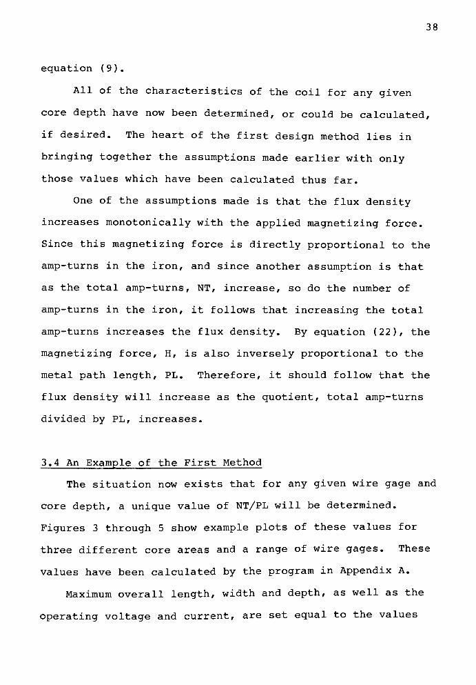
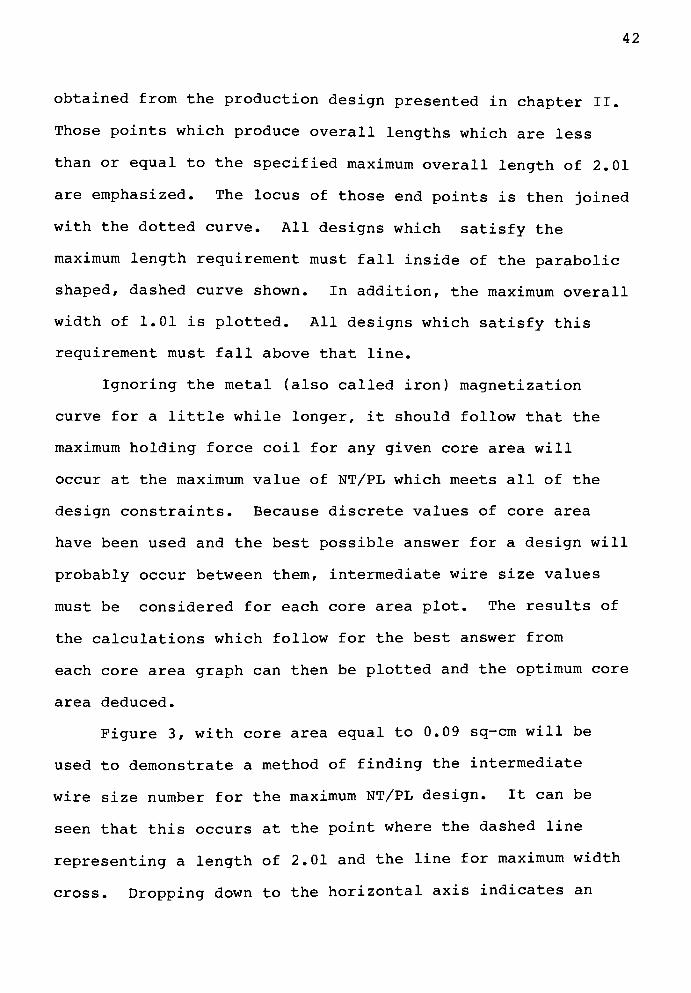
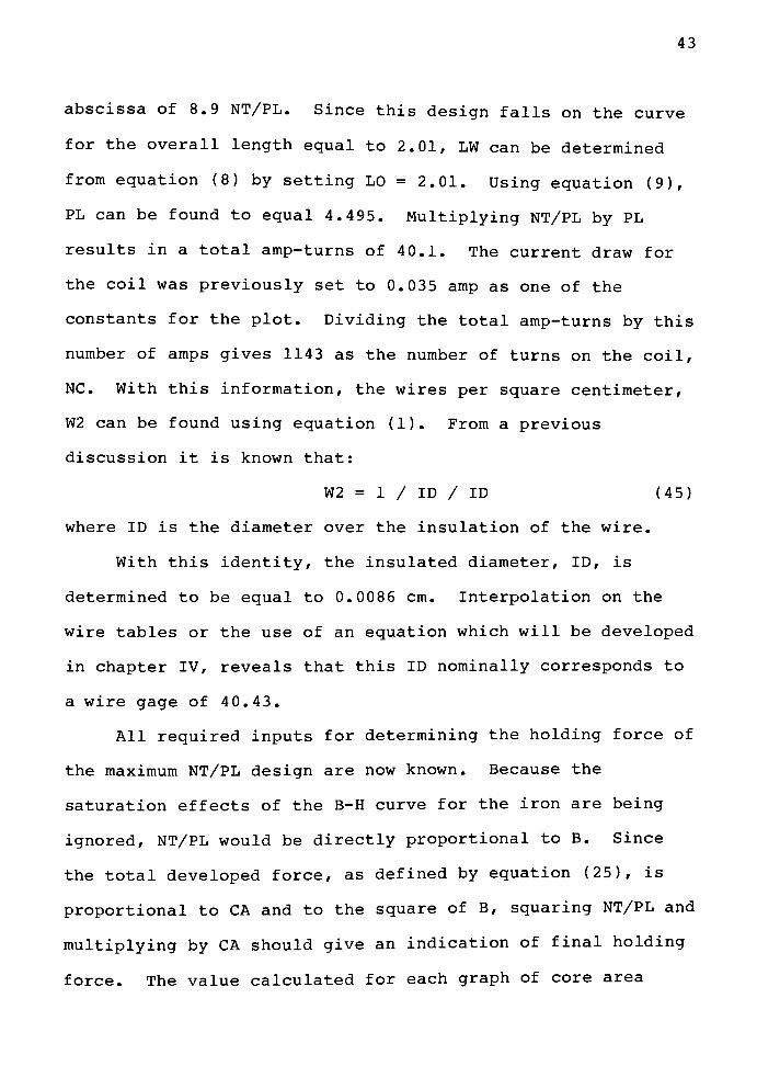
3.4 An Example of the First Method
The situation now exists that for any given wire gage and
core depth, a unique value of NT/PL will be determined.
Figures 3 through 5 show example plots of these values for
three different core areas and a range of wire gages. These
values have been calculated by the program in Appendix A.
Maximum overall length, width and depth, as well as the
operating voltage and current, are set equal to the values

39
"TO^ ro
O O O CD >
fN * V\OS
JA. O U\ ^ s3
>J ^ t^ 00 0
00
o
lo. <Js lr\
-3-
lr> Jf-
Oj OJ
J-
oo
t<^ r<v. f<\.1/N.
^ \f> nSt>-
o2
CMUJ
Ixl 0C
Oo Z>
< O) -
-CD o
3 ou_
LU II ,
0C <UJ
cc"
-co
<
*C_ UJ\^7
oc
o- |v-
^t
X
CO
h-
*>. o
o - - (2UJ
O_J
1 X
HLU
~ -
iO
o
-r^ 2
O
Z - -
<t
OC
* O \CO
in
c-l UJ ccsr
Q" -
rof^
^H 2
4,C0 - - 00 <
4
CC_)
\ Li_"
J.
,
h-
I 1 I I 1 1 1 I 1 I I I I I I ft
M+piM
OJOD
S^.a.Dr^CvJ N tO Cvl N iO M*
H t ^ ro.lOncvjMWW-r-^-
(ujo) Hld3Q3a03

40
2 <t
fs \S <DS UN
l<N
00ON
UN
f<N im(V fN
/<N J- UN
n kv
ON <- KN Us QOCvJ Ns ,-N ^ f". Jr Jr UN ">8 TO
ca
(wo) Hld3Q 3d03
CM
u
lO
CM
CM
<UJ
OC
<
UJ
OC
o
Q
O
X
HUJ
o
LU
Q
HCO
CC
(T>
--00
UJ
cc
U_
Is-
XI-
*>cf
o0^
--St
rO
if)
CC
|P+0+o
i*n
oo M+PIMas oj
I I I I I I I I I I I I I I |.oiP
i o uo^io m m
i+ &_-.: - <m p- m cm i^iocm^T X'TrOrOrOfOCMCMCMCM - -
^ OJOD
Q_
CM <t
f2

41
3
NN
! > KN OS IfsO t NO !
S *l-r-
<Ni mn
fc-* $
ON
a:
N
N
UN8 fc
- *!OJ
(JN 00U\ ooJXN ^S
<\j OJ
MIPim ..
-
|P+o+*
00
*N
<o*
,-
UN vO f-
_*- oo
QM+PIM
? > 2 2 3 OJOO
i I l i I I i i i i i i i i i ft
S-S+^t:10^ l^iOCM N m M*.*
v. ro ro rt rO (M N (M (M -- ,- ,-
(wo) Hld3Q3UO0
42
obtained from the production design presented in chapter II.
Those points which produce overall lengths which are less
than or equal to the specified maximum overall length of 2.01
are emphasized. The locus of those end points is then joined
with the dotted curve. All designs which satisfy the
maximum length requirement must fall inside of the parabolic
shaped, dashed curve shown. In addition, the maximum overall
width of 1.01 is plotted. All designs which satisfy this
requirement must fall above that line.
Ignoring the metal (also called iron) magnetization
curve for a little while longer, it should follow that the
maximum holding force coil for any given core area will
occur at the maximum value of NT/PL which meets all of the
design constraints. Because discrete values of core area
have been used and the best possible answer for a design will
probably occur between them, intermediate wire size values
must be considered for each core area plot. The results of
the calculations which follow for the best answer from
each core area graph can then be plotted and the optimum core
area deduced.
Figure 3, with core area equal to 0.09 sq-cm will be
used to demonstrate a method of finding the intermediate
wire size number for the maximum NT/PL design. It can be
seen that this occurs at the point where the dashed line
representing a length of 2.01 and the line for maximum width
cross. Dropping down to the horizontal axis indicates an
43
abscissa of 8.9 NT/PL. Since this design falls on the curve
for the overall length equal to 2.01, LW can be determined
from equation (8) by setting LO = 2.01. Using equation (9),
PL can be found to equal 4.4 95. Multiplying NT/PL by PL
results in a total amp-turns of 40.1. The current draw for
the coil was previously set to 0.035 amp as one of the
constants for the plot. Dividing the total amp-turns by this
number of amps gives 1143 as the number of turns on the coil,
NC. With this information, the wires per square centimeter,
W2 can be found using equation (1). From a previous
discussion it is known that:
W2 = 1 / ID / ID (45)
where ID is the diameter over the insulation of the wire.
With this identity, the insulated diameter, ID, is
determined to be equal to 0.0086 cm. Interpolation on the
wire tables or the use of an equation which will be developed
in chapter IV, reveals that this ID nominally corresponds to
a wire gage of 40.43.
All required inputs for determining the holding force of
the maximum NT/PL design are now known. Because the
saturation effects of the B-H curve for the iron are being
ignored, NT/PL would be directly proportional to B. Since
the total developed force, as defined by equation (25), is
proportional to CA and to the square of B, squaring NT/PL and
multiplying by CA should give an indication of final holding
force. The value calculated for each graph of core area
44
can then be compared and the best design found.
Unfortunately, the B-H curve cannot be ignored. Figure
6 shows both this assumed equation and the actual ideal
holding force, as a function of core area, for each of the
maximum NT/PL designs from Figures 3,4 and 5, as well as an
additional sample at a core area of 0.0625 sq-cm.
As can be seen, the curves agree closely when the
core area is reduced from the largest being considered, until
the maximum holding force is reached. The assumed equation
then continues to rise while the holding force drops back off
rapidly. Later examples with the final optimization method
will show that the best design occurs at the knee in the
force curve, where B no longer increases rapidly with
increased H, yet CA is as large as possible while still
permitting the high value of B to be achieved.
3.5 Conclusions
In conclusion, a core area of slightly less than 0.1225
sq-cm seems to be the maximum force design which is allowed
by the design constraints. The wire size will be slightly
less than 41.5, and the core approximately square. This last
conclusion comes from an examination of the values for CD and
CW next to each plotted point. Everything to the left of the
peak is square, while to the right there is a gradual
deviation from square. Since a square has the smallest
perimeter for a given area, examination of equations (3), (4)

45
Comparison Of High est Force Designs
Common Requirements :
DX=.635 WX--1.01LX = 2.01 C 1 =.285
C2-.07 BF--15
RW-1 R-0V=3volts Cls.Q35amp
H I I \t.07 .08 .09 .10 .11
Core Area(cm)'
figure 6
46
and (13), indicates that a square should maximize NT for any
core area selected. The constraint on overall width is
causing a deviation from this at larger core areas as seen in
Figure 5.
Taken collectively, figures 3 through 6 imply that the
solution found is unique. The parabolic curves of figures 3
through 5 look very much like conic sections. If these
graphs were replotted in force and stacked to create a three
dimensional figure, they would form a steep hill for each
wire size. Figure 6, which represents the locus of peaks of
those hills shows, that there is one which is definitely
higher than the rest. Thus, the solution can be considered
unique for a given set of constraints. The only time two
equivalent solutions would occur is if two different wire
lines in figures 3 through 5 crossed precisely at the maximum
solution point.
To determine the exact solution, several more charts
like Figures 3 through 5, would have to be generated until
the best design is found. If a whole number is required for
the wire size, designs would have to be limited to falling on
a wire line. One of the advantages of this method is that it
permits the designer to see graphically which direction to
move in to meet additional design restrictions. It can also
be seen which constraints should be opened up to allow for
more possible choices. For example, referring to Figure 4,
it can be seen that increasing the maximum overall width or
47
length, or some combination of both, would give a higher
force design, which would fall on an integral number wire
gage line. A case of incompatible specs could also be found.
It is conceivable that a set of constraints could exist where
no feasible designs could be found. The graphical approach
shown would indicate that and the direction of changes for
solving the incompatibility could be seen.
The method also has some disadvantages. One is that
the overall depth has been set to the maximum. Using
overall width as an example on Figure 4, had it been set to
2.0, the best design would have occurred at an overall width
of 1.134 and not the maximum 2.0 allowed. In addition,
number 41 wire would be used instead of 41.5. Thus, the
final design is not always at the maximum space allowed.
Similarly, the best design may not always be at the maximum
overall depth, but rather at some other value. To determine
if this is the case, another set of (3) graphs at some lower
maximum overall depth would have to be constructed and
compared to the first. At least three sets would have to be
constructed to find the best operating point.
Likewise, a change in any of the other givens , such as
voltage, would require a new set of charts unless the current
is scaled proportionally. The biggest drawback is that the
method does not meet the basic goal of this project, which is
to have the method independent of theusers'
knowledge of it
or magnetics. The method described is excellent for use by a
48
non-novice who wants to determine what options are available
for changing a final design.
One feature, which was not possible to show with the
scale of the graphs in this paper, is the placement of the
overall length dimensions next to each wire curve at each
core depth. Originally, this work was done at a larger scale
to permit this, and a better feel for the rate of change of
the length could be obtained. With the graphs shown, the
2.01 limit line is treated as an absolute. It is necessary
to refer to the computer printout for the intermediate
values, and information is lost in the transaction.
While it might be possible to computerize the graphing
function, and thereby reduce the time required for the
method, it was felt that other methods would be better suited
for use on a digital computer. As a result of this fact,
plus the combination of disadvantages already discussed,
another approach has been pursued for a user friendly,
computerized design method. The presentation of it will be
made in the next several chapters.
CHAPTER IV
CURVE FITS
4.1 Introduction
Before any automation can be attempted, there are
several pieces of information which are either in tabular
or graphical form that must be curve fit. The alternate
choice would be to have a series of look up tables. These
would require a search and interpolation each time they are
referenced. Clearly, a good curve fit has the faster
execution time and does not suffer from the inherent round
off present in any tabulated data.
4.2 Bare Wire Diameters
The first item of concern is the diameter of the bare
wire, since most of the wire constants are related to
this. The aim is to find an equation which accurately
relates wire gage number to the corresponding wire
diameter. Such an equation can be generated when it is
recognized that the wire diameters follow a geometric
progression (Ref 7). Thus, the diameter ratio of two
successive gage number wires is a constant. In the
discussions which follow, initial calculationswill be in the
english system of units to simplifycomparisons with the
standard wire tables. Conversions will then be made to the
49
50
cgs system for compatibility with the other equations.
Because the data presented in standard wire tables has
been rounded to the nearest 0.0001 inch, the ratio of
neighboring wire number diameters will appear to vary
slightly. One method of finding the true value would be to
determine every ratio over the range of wire sizes of
interest and then compute their average. A simpler method is
to choose two wire gages which are n numbers apart, find the
ratio of their diameters and then take the nth root of that
ratio.
This second method is the one used. Number 0000 wire
has a 0.460 inch diameter while #36 wire has a 0.005 inch
diameter. The ratio of the diameters is 1/92, and they are
separated by 39 wire gages. Taking the 39th root of 1/92
yields a constant of 0.890525717. To relate the wire gages
to the corresponding diameters, it is necessary to solve the
following equation, which is based on the geometric
progression relationship described earlier.
(dia of #n)/(dia of #m)=( 0. 890525717)** (n-m)
Setting n=36, where the diameter is known to be 0.005, and
m=0, and solving for the diameter of #0 wire gives the
desired final equation.
(dia of #n) = 0.324860745 * (0.890525717)** (n) (46)
This equation has been checked against all of the wire sizes
from 14 through 44 and has been found to have an average
error of -0.005% with a maximum error range of -1.12% to
51
+1.44%. This"error"
is actually roundoff in the table
values. Appendix G contains a table which compares the
diameters found by equation (46) and standard wire table
values. Also in that Appendix is a copy of a standard wire
table page for single build, enamel coated wire. Multiplying
the values obtained in inches by 2.54 gives the diameter in
centimeters.
4 . 3 Ohms per Unit Length
The bare wire diameter can now be used to find the
resistance of any wire diameter by the following equation.
(R8) R = k * L / A (47)
In equation (47), R is the resistance in ohms, k is the
resistance of 1 mil-foot of wire in ohms, L is the length of
the wire in feet and A is the area in circular mils. A
circular mil is simply the square of the diameter of the wire
which is measured in mils. The constant k has a numerical
value of 10.372. For the coil equations developed, it is
desirable to find the ohms per inch rather than the total
resistance and have the diameter measured in inches rather
than mils. Equation (47) can be rearranged to be in the more
useful form of equation (48) by converting L to inches and A
to square inches.
OI = (8.64333333E-7) / WD / WD (48)
Here OI is the ohms per inch and WD is the wire diameter in
inches. Equation (48) can be used to convert from ohms per
52
inch to ohms per centimeter, OC.
OC = 01 / 2.54 (49)
As a check, resistances found by equation (48) have been
compared to the standard wire table values. Appendix G
contains a summary of this analysis. The average error is
+0.03% with a range of -2.79% to +2.28%. There is no trend
to this error since the sign is random throughout the wire
range checked. Therefore, the equation and constants can be
considered an excellent match.
4.4 Insulated Wire Diameters
No information could be found for calculating the
overall diameter of the enamel insulated wire. However,
equation (46) can be rearranged to produce equation (50).
IN = LOG(ID/0. 324860745) / LOG ( 0 . 890525717 ) (50)
In this equation, IN is an effective wire number for the
insulated wire and ID is the diameter over the insulation.
The insulated diameters, ID, can then be plugged into this
equation to arrive at a resultant effective wire number. If
the insulated wire gage values are then plotted against their
corresponding bare wire diameter gages, WG, a straight line
results. The line has a slope of 0.967 and an intercept of
0.221. Thus, an effective wire number for the insulated wire
can be determined from the bare wire gage number.
IN = 0.967 * WG + 0.221 (51)
The overall diameter can then be found from equation (52).
53
ID = 0.324860745 * 0.890525717 ** IN (52)
A comparison between insulated diameters found by
equation (52) and those in the standard wire tables is shown
in Appendix G, and indicates a slight error. To get a
perfect match with the wire tables, the constants would need
to be adjusted slightly. The average error is +0.826%, which
means that the calculated diameter is larger than the table
value by that amount. This has a range of -0.67% to +3.68%
with the larger errors occurring at the larger wire gages.
The insulated wire diameter is used only in equation (45) to
find the turns per unit area. An overestimate of the wire
diameter by 2% will only reduce the calculated number of
turns per area by 4%. The fact that this is in the direction
of helping the coil winder and that some books recommend a
reduced random wind factor at higher gage numbers (Ref 9),
lead to the decision not to adjust the constants. More
significantly, the calculated values fall well within the
dimensional tolerances allowed in the tables.
4.5 Thermal Coefficients
The last fit to be discussed in this section is for the
heat dissipation coefficient, K, versus the watts per square
inch of effective coil radiating surface. Using data taken
from a graph (Ref 4), which was plotted between 0.2 and 0.8
watts per sq-in, an exponential equation was assumed and then
adjusted with a slope equation. The resulting equation

54
agrees extremely well with the data taken, but may not apply
outside the range checked.
LK =
exp(PA)/(107.23*(PA+0.194)*(PA+0.194)+191.5) (53)
LK is the dissipation coefficient and PA is the power per
square inch of surface area.
4.6 B-H Curve Digitization
The discussion of the choice for entering the
magnetization curve will be left for Chapter VIII when that
program module is presented in detail.
CHAPTER V
SECOND OPTIMIZATION METHOD: PROGRAM OVERVIEW
5.1 Introduction
The complete program is a user friendly set of five
program modules, stored on a single 5-1/4 inch floppy disk,
which are in repeated interaction with one another. They are
written for use on an Apple 11+ computer equipped with a
single disc drive and monitor. A dot matrix printer with a
graphics dump driver, such as the Grappler, is also
recommended but not required.
The purpose of the complete package is to provide a
method of designing the highest holding force horseshoe type
D.C. electromagnet which will fit within given space
constraints and is subject to other user defined limits. It
will also analyze an existing coil design and display the
results on a monitor or printer. One of the primary goals in
developing this program is to make it as user friendly as
possible. The user should not be required to have more than
a minimal knowledge of magnetics, the program, or its inner
workings. As a result, the graphics capabilities of the
Apple computer are heavily utilized. In addition, single
keystroke entries are used wherever possible, and user
responses are checked against possible correct responses. In
the event of entry errors, the program will ask for the
55
56
necessary information again. The program works extremely
well and meets all the initial goals.
5.2 Program Structure and File Management
The reader is referred to Figure 7, for a better
understanding of the module inter-relationships. This
figure is a block diagram showing how the modules are
connected and the direction of information flow. Each block
will be discussed separately in its own chapter, while the
purpose of this chapter is to look at the overall structure.
One item, which stands out in the flow chart, is the
frequent use of sequential files. These are used to pass
information from one module to another. The file RUN TYPE
contains only four pieces of information. Its purpose is to
help each module determine which task should be performed
from its list of several possible tasks. These four items
are: l)The bobbin style being considered, AA. This
information is used to choose the correct picture to draw or
make minor equation changes as dictated by the bobbin and
core configurations. 2)Type of study, TS, helps to choose
the order of module execution. In addition, it works in
conjunction with AA to draw the correct pictures. There are
two basic types of study, design and analysis. Depending on
which module is being exited, however, this variable can take
on any of four values. 3)Entry type, ET, can take on any of
three values. A"one"
indicates that data will be entered

57
Introduction
(page 1) 3.3 K
\ \
(RUN TYPE) 'SHAPEF1LE 0.5K
I ./
Input/Output
(PAGE 2-A) 16.5K
I
(>F1NAL DESIGN)
(run type) (run type)
i i
(dtest coil) (@>test coil)
IAnalysis
ii.ik
CoilDesign
19.9K
->(@testcoil)
(run type)
B-H Entry
(B-H) 6.4 K
(run type)(
^MATERIAL file5)
(DTESTCOILD(run type)
L
NOTE-
_J PROGRAM MODULES
IN RECTANGLES,SEQUENTIAL FILES
HAVE RADII
PROGRAM FLOW
FIGURE 7
58
from the keyboard,"two"
is temporarily used in some modules
to view the catalog, and"three"
is for entry from a disk
stored file. 4)Name of file, NF$, is the title of the design
being studied. It will eventually be the name of the @FINAL
DESIGN file on the flow chart, as well as, appear on the
input and output drawings for the coil.
The second frequently used sequential file is named
@TEST COIL. This is a working file for all the coil
information, and is added to or modified by each program
module. A file does not take on its final name until the
user is finished with it and decides to keep it on the
disk for permanent storage. This avoids cluttering up the
program disk with undesirable intermediate designs.
JMATERIAL FILE is a generic name for the material
specification file. It contains the information describing
the initial magnetization portion of the B-H curve for the
material named by the title of the file.
One item of note is that all design files are preceded
by an @, while all material files are preceded by a square
right hand bracket in the disk catalog. The average user
will be unaware of this feature, and when entering material
or design names, has the option of placing the prefix on the
name. However, the program will automatically add the proper
prefix if it is not present before storing it on disk, but
subtracts it before putting the information on a final
drawing. The reason for the prefixes is that the sequential

59
files for this program are very short. As a result there
could be up to 105 files on any design disk (limited by the
number of file names allowed on a disk, not by disk
capacity). To make it easier to find materials or designs in
a catalog listing, the prefix has been added so that the user
can quickly scan for the proper file type, and not have to
read each name in its entirety. Appendix I shows a sample
catalog listing.
5.3 Memory Management
An obvious question might be, why use these sequential
files at all? Why not have one large program instead of five
smaller modules? The answer can be found in the diagram of
Figure 8, which shows three memory maps of the Apple 11+, to
a scale of 0.1 inch per IK of memory. One of the ground
rules when developing this program was that it had to be
capable of running on a standard Apple II computer equipped
with a single disk drive, but not necessarily additional
memory or other special equipment. The left column of the
memory map shows the standard configuration. HGR1 and HGR2
are the two high resolution graphics pages and cannot be
moved. If a program is not using either, that memory is
available.
If, however, graphics are to be used, then the block of
memory for the page being used cannot be utilized or crossed
by the resident program. In addition, under normal

MEMORY MAP
60
48K(49152)-
38K(38912)
24K(24576)~
16K06384-
8K (8192)
2K (2048)0
VARIABLE
STORAGE
HGR2
HGR1
BASIC
PROGR.
<CC
O
OCC
Ql
CO
<
o
o
OC
Ql
HGR1
UNAVAILABLE
NORMAL
APPLE
COIL
DESIGN
ALL
OTHERS
1
/PAGE 2-A
^ANALYSIS}B-H
PAGE1
1^(2544)
SHAPE
FILE
FIGURE 8
61
circumstances, a Basic program is entered starting at the
first available memory location which is 2048 ($0803).
Therefore, if programs are written in Basic, and HGRl is
used, the length of that program is limited to 6K. HGR2 can
be written on instead of HGRl to increase that amount to 14K,
but this has several drawbacks whose details are not
important to this discussion.
Returning to Figure 7, it can be seen that all of the
programs except the Introduction exceed the 6K limit. Since
HGRl is a basic premise on which the concept for this user
friendly program is based, and the language being used is
Basic, an alternate approach or computer is required.
Fortunately, an alternate approach is available.
The default starting address for an Applesoft program
can be altered by Poking the new values into memory
locations 103 and 104. Final results are the two memory
maps shown to the right of the normal Apple column in Figure
8. The starting address for all of the program modules,
except the Coil Design program, is placed above HGRl.
Unfortunately, there is an upper limit to programs
placed above HGRl, which is determined by the disk operating
system (DOS). Although the previous situation has been
improved by an expansion of available program space to 22K,
all of the program modules cannot reside in memory at the
same time because of their combined sizes. In addition, the
Coil Design program is still too big to fit above HGRl and
62
have enough room for its required variable storage. Thus,
the reason for the final memory management. If each module
could operate as a stand alone program, and if the coil
design module did not require graphics, then there would be
sufficient memory capacity in a standard Apple computer to
accommodate the project. The sequential files behave like a
COMMON statement in Fortran, and also can be used in a manner
similar to the EQUIVALENCE statement in Fortran. This last
feature was necessary because of the use of an existing
program for the design module. Conflicts of variable names
would have resulted unless equivalence could be used. The
alternative would be to change variable names, and thereby
avoid conflicts. Not very desirable for many reasons!
5.4 Shapefile
The final item of discussion, before describing each
module in detail, is the block called SHAPEFILE (Ref 10).
This contains the character generators for writing on the
high resolution graphics pages. Normally it is not possible
to write text on the graphics screens. To overcome this
deficiency, the programmer must generate the character set,
and store it in a shape table for later use. This is the
function of SHAPEFILE. It has been stored at the bottom of
memory to safeguard it against the possibility of being
overwritten by stored variables and programs. The starting
address for COIL DESIGN is placed immediately above this.
63
5.5 Final Note
At this point, the memory capacity and its organization
has been established. Now upper limits can be placed on the
program sizes and the programming for the problem can begin.
Each program module chapter contains a section
describing any computer dependent commands used in that
module. In the companion Appendix, a variable cross
reference and program length message are listed along with
the complete module code. These pieces of information are
intended for the individual interested in modifying a program
or transferring it to another computer system.
Because many of the commands are related to the graphics
required for user friendliness, the simplest method of
transfer to another system would be to eliminate these
entirely. While this will remove one of the main features of
the program, it will leave an engineering tool which will
perform its intended task well. The drawback will be that
the user will have to rely on word prompts rather than
pictures.
CHAPTER VI
PAGE 1 PROGRAM MODULE
6.1 Module Purpose
This module serves as an introduction to the design or
analysis process, and determines the path which will be
taken through the block diagram of Figure 7. Since the
program is intended to be for use by individuals who may not
be familiar with the terminology used, a purely word based
prompting technique is undesirable. It is said that a
picture is worth a thousand words, and is, therefore, the
medium of choice when maximum user friendliness is desired.
6.2 Program Flow
Figure 9b, shows the drawing generated by PAGE 1, on the
monitor after clearing the title screen, 9a, it had created
previously. Once the picture has been displayed, the user
is asked to enter the coil type to be studied. When any key
is pressed, the program checks to make sure it is either a
1,2,3 or 4. If not, the question is repeated. If so, the
user is asked to confirm the entry with a Y/N response.
Rather than describe the user friendliness features in
each module, the blanket statement will be made here that
for every entry, maximum user friendliness has been
considered. Single keystrokes are used whenever possible,
64
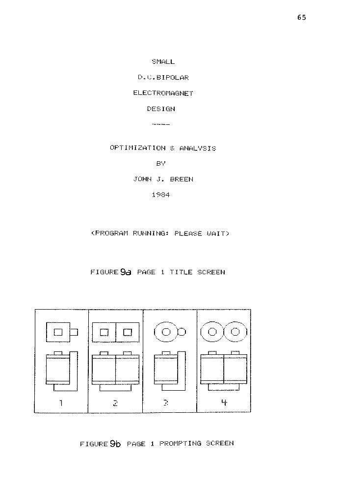
65
SMALL
D.C. BIPOLAR
ELECTROMAGNET
DESIGN
OPTIMIZATION S ANALVSI;
BV
JOHN J. BREEN
1984
< PROGRAM RUNNINGS PLEASE WAIT .'J
FIGURE 9d PAGE 1 TITLE SCREEN
? :: ? D ( (J P ( O I o )
1 1 1 1r
1 ... ,m m r-,,
1h-
i 1 \ !
1 iL
H-
FIGURE9b PAGE 1 PROMPTING SCREEN
66
and prompts are clearly worded. If possible, the program
checks for the validity of a response and reprompts if
warranted. Default values are suggested in many
questions, and a single strike of the RETURN key will accept
the default. While there are certainly some potential
loopholes in this logic, great pains have been taken to
account for likely user errors and questions.
Continuing with PAGE 1, the next prompt asks if the user
wishes to analyze or design a coil. This generates a value
for the variable TS.
The final set of questions relate to the study name,
NF$. When the design name is entered, PAGE 1, will add the @
sign if it is missing, and then checks the disk to find if it
already exists. If it does, the user can choose between
overwriting the file from the keyboard, entering a new name
after reviewing the catalog, or entering the information
already stored in that file from the disk. If the file does
not exist, there is a choice of entering the new data from
the keyboard, or reviewing the catalog to find a file which
does exist. From these final prompts, NF$ and ET are
generated and the values stored in the file RUN TYPE.
The screen now clears and a message appears that the
input/output module is being loaded, so have patience. This
completes the function of the short PAGE 1 program.
67
6.3 Special Program Notes
A program listing followed by a variable cross reference
listing can be found in Appendix B. This cross reference
lists each variable used in the module and the line numbers
in which it occurs. The file length is also listed if a
rearrangement of memory is considered.
Since this program is basically a picture generator, its
conversion to other systems is not likely. Most of the
related commands are unique to an Apple computer. Therefore,
if it is desirable to transfer the program in this project to
a different system, it would be best to eliminate this module
and only ask the limited number of questions needed with word
prompts. These should be placed at the front end of the PAGE
2-A module or its equivalent.
CHAPTER VII
PAGE 2-A PROGRAM MODULE
7.1 Introduction
This module is the central controller and input/output
manager for the entire program concept. It generates the
coil pictures on which the various dimensions are displayed,
and organizes any information which must be passed to the
printer, monitor, disk or another program module. The size
of the program is dictated by the graphing and user friendly
features it contains rather than its basic functions.
During the keyboard entry phase of the program, the
graphics become interactive. When the coil drawing is first
generated on the screen, no dimensions are present. Only the
dimension lines, arrows and variable identifiers are in
place. As each entry is made, it is placed on the drawing at
its proper location. In a similar manner, when a change is
made, the screen immediately erases the old dimension and
inserts the new one. This dynamic screen, in conjunction
with good word prompts, make the program extremely easy to
use, and eliminate the need for operating instructions.
7.2 Program Size Considerations
The demands on this module, for the memory space
available, are significant. Because graphics are used
68
69
extensively by it, the module has to reside either above or
below the high resolution graphics page one. This
immediately places an upper limit on its size.
The biggest factor on size is the graphics requirement.
If the eight individual pictures required were stored on disk
as separate files, they would require 34 sectors apiece for a
total of 272 sectors. This amounts to half a disk just for 8
pictures. Since a single drive is a requirement of the
program design, this storage is unacceptable. A second
alternative is to have a separate picture generating module
for each drawing. This is again not very compact or clean.
By a careful design of the eight pictures and the
locations of their dimension lines and related dimensions, a
more compact form results. The program is set up to reuse
as many lines of code as possible. To this end, whenever a
picture is required, all lines common to every drawing are
drawn first, followed by a branch to the lines for round or
square cores. A series of subsequent branches for drawing
all those features common to everything which follows it are
executed, until the correct picture is completed.
A similar problem occurred with the entry of data from
the keyboard or disk. Sixty potential pieces of information
must be managed, though only about a third of them are
required for any given display. Subroutines for each entry
are used. For simplicity, a different calling block is used
for each type of picture.
70
Finally, the change routines which are required take a
large amount of code. This has been handled by a careful
choice of the order in which the change questions have been
arranged in the program. A branching technique, similar to
the drawing one mentioned, is then used. Whenever a
dimensional change request is made by the user, the program
searches through a list of variable names. When the desired
variable is found, the corresponding dimension on the drawing
is erased, using the same program lines which originally put
it there. The user is then told what the current value is
and is asked to enter a new value. Wherever possible,
default values are suggested, and will be chosen with the
single stroke of the return key.
The result is a very efficient program, which handles
all eight drawings, sixty pieces of information, keyboard
entry, disk entry, module execution management, and changes,
as well as, output requirements in less disk space than would
be occupied by two graphics pages. The drawings, which will
be discussed and shown in detail in Chapter XI, are very
readable and serve their purpose well.
7.3 Other Functions
Before permitting an exit to the ANALYSIS module, PAGE
2-A, checks to be certain that the material file specified
exists. If it does not, the user is given the option of
either changing the material or branching to the B-H module
71
for material entry. Otherwise, the analysis is started.
In addition to the material check, many others are
made before an exit to the COIL DESIGN module can be
executed. All maximum and minimum values are checked to be
certain that they are not inverted. In addition, some basic
calculations are made to be certain that the maximum wire
space allowed, in combination with the maximum gage number
and voltage, will permit the maximum coil current
specification to be met. More fundamentally, a check is made
to be certain that the combination of requirements allows for
any flange width or winding length at all. Should any of
these incompatibilities exist, an error message results, with
suggested corrections. Otherwise, the specifications are
considered acceptable, and the coil design can almost begin.
Reference to Figure 8, reveals that the COIL DESIGN module
must reside at a different location in memory than PAGE 2-A.
Therefore, the last function performed by this module is to
relocate the starting address for the next Applesoft program.
7.4 Special Programming Notes
This module is almost exclusively machine dependent.
All of the graphing functions are unique to the Apple
computer, as are the sequential file management instructions
and memory location commands. Therefore, transfer of this
input/output module to another system is not recommended.
Instead, the programmer is encouraged to write a different
72
module.
Appendix C, contains a complete program listing in
addition to the length message and variable cross-reference.
CHAPTER VIII
B-H ENTRY PROGRAM MODULE
8.1 Program Function and Flow
The purpose of this module is to provide a simple means
of entering a D.C. magnetization curve, like the examples
shown in Figure 2, and Appendix F. It does not assume that
the operator even understands what a B-H curve is. It is
only necessary that he has the appropriate information for
the material of interest, plotted on semi-logarithmic axes,
available for digitization. Units of entry can be any that
the user chooses. Values are converted to kilogausses and
oersteds, however, before they are saved to the disk.
Data is checked as it is entered to verify that it
follows the rules of a monotonically increasing function.
Violations of these rules result in a flashing error message
and a repromt for the value requested. Up to 40 points may
be entered, and are continuously displayed in chart form on
the monitor screen. Figure 10, shows a sample of the entry
screen for the 50/50 NI-FE (SOLID) file. On the monitor, the
headers would show in inverse. An entry of E, for any value,
signals the end of the entry process and the start of the
editing phase.
Full editing features are supported, including add,
delete, insert and change. When one of these functions is
requested, the table of values is adjusted appropriately and
73

74
CHI13)
2 7*
.83
04
2 1 .')
223)
335. 855 2 n
">^ 233)
4.). 1 6. 5 24 >
5.':>. 15 y n 5 253)
t, ;jn 3 10 .5 2'
?'y n 12 27 y
s > "7 cr
13 .5 28 3)
9 3'-' "IfCT'
15 29 3)
leo 100 15 .4 30 3)
n> 4506 15 .41 313)
12> 323)
13 3) 33 .')
14 3) 34 3)
153) 353)
1635 36 .)
17 3) 37 3)
183) 38 3)
19 3) 393)
20 ':> 40.)
El El
10ALLIES IN OERSTEDS? KILCiGAUi
FIGURE lOsB-H ENTRV PAGE SHOWING 50.-"50 NI-FE < SOL ID 3)
75
prompts for the necessary information are displayed.
When the data entry process is completed, the
information is stored on a disk under the name of the
material.
This name is preceded by the right square bracket prefix
mentioned in Chapter V. If the file already exists, the
program will verify that it should be overwritten before
doing so. Renaming of the file is allowed at this point, if
the existing file is to be kept.
After the saving process, control is returned to PAGE
2-A, unless more materials are to be entered. Should more
entries be required, or an existing file need editing, the
module will restart itself and begin the entry process again.
8.2 Basic Concept
It was felt that the entry process had to satisfy
three fundamental requirements, the first of which is user
friendliness. Some curve fitting techniques require careful
selection of the data points to obtain a good match. This
demands a full understanding on the part of the user of the
technique being used, which is a violation of the user
friendly concept.
The second two requirements are related to the computer.
First, the method must result in an accurate representation
of the actual B-H curve. Finally, whatever method is chosen
must allow for easy interpolation between inputted points.
76
One of the difficulties with many curve fitting
techniques is that they agree at the given points, but
deviate considerably between them. It is also possible
that one technique would not apply for all possible
curves desired. This might require decisions on the part of
of the user for deciding which method would best apply. This
is again anti-user friendly.
Close examination of the large variety of curves shown
in Appendix F, reveals that they can be approximated quite
well with a minimal number of straight line segments.
Assuming that these are a good representation of possible
curves, then if straight lines work for them it would satisfy
all of the requirements and be the simplest to execute and
understand.
Several curves were approximated, and most required less
than 10 line segments for the process. The Apple monitor can
conveniently display 4 0 data points in a static chart, and
thereby define 3 9 line segments. Since this exceeded the
typical expected number by a wide margin, 40 was chosen as
the maximum number of data points, and the foundation for the
program format settled.
8.3 Observations on the Method
Once again referring to Figure 10, it can be seen that
the curve for 50/50 NI-FE (SOLID) has been represented by
only 10 line segments. If plotted against the original curve
77
in Figure 2, the points along the line segments are almost
indistinguishable from the original. Similarly, cold drawn
carbon steel was approximated by 8 segments and oriented 3%
silicon strip by 12. The original curves for these materials
can be found in Appendix F.
The method is very quick and easy, and requires little
instruction. The accuracy is well within that which would be
obtained by reading the curves for a manual analysis.
The method, therefore, meets all the stated requirements and
works well with the other program modules which use the
information.
8.4 Special Programming Notes
Generally, the program is straightforward and warrants
little mention. Its complexity is determined more by the
user friendly requirement than the function it serves.
One Apple related trick is needed to make the concept work,
however. This is the POKE 34, X statement found in subroutine
1500. The function of this statement is to produce a static
display from the top of the screen down to line number X.
All lines below X scroll normally. The static display can
then be written to, using horizontal and vertical tabs.
CHAPTER IX
ANALYSIS PROGRAM MODULE
9.1 Program Function and Flow
The primary function of the ANALYSIS program module is
to analyze the characteristics of a D.C. bipolar electro
magnet whose physical dimensions are known. The equations
used are essentially identical to those presented in Chapter
II. The resulting calculations are displayed on the monitor,
printed out, or not shown at all, based on a user selected
option.
A second (optional) function is to repeat only those
calculations which apply to holding force over a user
selected range of voltage and air gaps. This shows the
sensitivity of the force to those parameters. Based on the
range of force and voltage, a graph of this data is scaled
and plotted to fill the monitor screen. If the print option
has been chosen, a copy of the graph is sent to a dot matrix
printer. In addition, the data used to generate the graph is
listed.
Before exiting to PAGE 2-A, where a picture is generated
of the analyzed coil, all of the data, with the exception of
the sensitivity information, is stored in the @TEST COIL file
on disk. As shown on Figure 7, the analysis module may be
called directly by PAGE 2-A, when TS is set to unity in the
78
79
PAGE 1 program. It may also serve as an intermediary between
the COIL DESIGN and PAGE 2-A modules.
9.2 Assumptions and Constants
Several assumptions are made when making the temperature
related calculations. One is that the core is in poor
thermal contact with the windings and, therefore, has no heat
capacity. Another is that the surrounding air temperature is
at a constant 20 degrees Celsius. A final assumption is that
the air is free to circulate about the entire coil winding
surface area. This last assumption may not be valid for a
double bobbin design when the coils are in close proximity
with one another. It may also not apply if the coil is
mounted in such a way that one or more faces are effectively
insulated against thermal convection.
These combined assumptions are the basis for the choice
of the equation which determines LK, the heat dissipation
coefficient. If some of the surface area is insulated, a
modification of the surface area equation would correct for
this. However, if any of the other factors do not agree with
the assumptions stated previously, Ref. 4 should be consulted
for a more detailed explanation of required changes.
The program will also point out those constraints which
have been violated by the design, if constraints have been
specified. To allow for accumulated round-off effects, an
arbitrary error threshold of one percent must be exceeded to
80
set off a violation flag.
During the initial calculations, a check is also made of
the number of turns specified, versus the potential number of
windings for the bobbin. Any difference greater than five
percent will result in a message being displayed. This will
tell the user if the bobbin is over-or under-filled, and
asks which of three options should be executed. These are to
either accept the over/under-fill condition by setting the
winding width to the calculated value, adjust the winding
factor to fill the winding space, or review the calculations.
Based on the choice made, the ensuing calculations are
modified accordingly.
9.3 Amp Turn Distribution Calculations
With the exception of the amp-turn distribution
calculations, the equations and methods used in this program
module are identical to those presented in Chapter II. The
reader will recall that this distribution of the mmf between
the iron and air is determined by a series of trials which
consist of a guess, followed by an involved calculation
sequence. While it is true that the computer can carry out
this iterative process without difficulty, it can be time
consuming. For the ANALYSIS module this is not a big concern
since the iterations are only carried out once. In the COIL
DESIGN module, however, which will be described in Chapter X,
these iterations must be carried out twice per independent
81
variable per basepoint in the search process. Depending on
the number of base points required, the time consumed can
become an important factor. For consistency, the ANALYSIS
and COIL DESIGN modules should use the same search technique.
As a result of the design module concerns, a technique
for finding the amp-turn distribution has been developed.
The result is one equation with one unknown, requiring few
iterations to solve. The equation manipulations required and
simplifications made are as follows. Figure 11, shows the
terms and graphical representation of the concepts described
in this section. Most texts use the Greek letter phi to
represent flux. To be consistent with the programs
presented, however, F will be used, with variants of FL and
FU.
In the example problem presented in Chapter II, one of
the calculations which had to be made during the iterative
loop was dictated by equation (23). This was necessary
because a relationship between the flux density, B, and
magnetizing force, H, was known for both the iron and air
paths. For the air, equation (14) indicated that B and H
were equal in the cgs system. For the iron, some function
defined by the initial magnetization curve described the
relationship. Equation (23) was used to tie these two known
relationships together.
The beauty of the B-H relationship is that it is
independent of part geometry. This allows the publication of

82
xnid
9V*VG-V0*T8-XrfU
u_
83
a
was
one curve for each material. However, to simplify the
discussion which follows, it would be better to have
relationship between flux and H. In section 2.5, it
stated that flux must be conserved. At the pole/air
interface, the flux is not being divided, but is only
changing medium. The flux in the air, therefore, must equal
the flux in the iron. By equation (17), the flux is equal to
the flux density. B, times the area through which it is
passing. Since the core area and gap area are being treated
as constants, it is possible to scale the B axis for both the
air and iron by their appropriate areas, so that both HA and
HI will be plotted against a common vertical axis of flux.
For the air, a combination of equations (14) and (17)
indicates that there is still a straight line relationship
between flux and H.
FLUX = AG * HA (54)
Plugging in equation (15) for H, gives the desired end
relationship relating flux to the amp turns in the air, NA.
FLUX = (AG * 0.4 * PI / G) * NA (55)
This line is shown in Figure 11, and its slope is defined by
the quantity in parentheses in equation (55).
For the iron, the relationship between B and H has been
reduced to a series of straight line segments, when H is
plotted on a logarithmic axis. Taking the logarithm of both
sides of equation (15) gives equation (56).
LOG (HI) = LOG (NI) + LOG (0.4 * PI / PL) (56)
84
With equation (56), an identity now exists which will allow
the flux to be plotted against the logarithm of the amp turns
in the iron. This plot will still be a straight line for any
segment in the material file, and is also drawn in Figure 11.
It must be remembered that the horizontal axis for the amp
turns in the iron is logarithmic, while that for the air is a
cartesian grid.
The end points of the line segments for the B-H curve of
the iron are stored in the material file, and are, therefore,
known. From the relationships presented in Chapter II, the
flux and number of amp turns in the iron and air can be
calculated from these values. These are indicated by the
dotted lines in Figure 11. Once the iron and air amp turns
are defined at an end point, the total number of amp turns at
that point is simply their sum. The computer can be used to
scan through the material file to find a pair of end points
which bracket the total number of amp turns available. That
point will correspond to some as yet unknown flux, air amp
turns and iron amp turns. This is also shown in Figure 11.
Through the use of similar triangles, the relationships
defined by equation (57) can be found.
(LOG (NIa) - LOG (Nil)) / (LOG (NIu) - LOG (NIl))=
(Fa - Fl) / (Fu - Fl) =
(NAa - NAl) / (NAu - NAl) (57)
Equation (58), is determined by applying equation (20),
for the aim point being sought.
85
NIa = NT - NAa (58)
Setting the first and last identities of equation (57) equal,
and applying the identity in (58), gives equation (59).
LOG (NIa) + AA * NIa = KK (59)
where AA = (LOG (NIu) - LOG (Nil)) / (NAu -
NAl) (59a)
and KK = AA * (NT -
NAl) + LOG (Nil) (59b)
All of the variables in equation (59) are known, with
the exception of NIa. In the computer programs presented, a
modified interval halving technique is used to find the aim
number of amp turns in the iron. In addition, the equations
in the program are slightly messier than the ones presented
here. The simpler form was found too late to be incorporated
in the programs. Using the identities available in this
paper, however, it is easy to show that the two solutions are
identical. The details will not be presented here.
As an experiment, the Newton-Raphson method was tried in
place of the bisection technique with no improvement in the
error. Since the bisection technique gives acceptable
answers and the final listings were complete, the listings
shown contain the bisection method. Newton-Raphson would be
guaranteed to converge, based on the physical requirements of
the variables in equation (59). Errors, resulting from
round off and any techniques used, are shown by a difference
in the two values of total amp turns printed out in the
sample runs presented in Chapter XI.
86
9.4 Special Programming Notes
Appendix E, contains a listing, program length message
and variable line cross reference of the ANALYSIS module.
Aside from the file management techniques, common to all of
the programs in this project and the graphics functions,
there are no equipment dependent commands. For this reason,
the module can be easily converted to other systems.
CHAPTER X
COIL DESIGN MODULE
10.1 Introduction
The purpose of this module is to design the maximum
holding force coil, which will meet all of the user specified
constraints. If no such design can be found, a design, which
satisfies as many of the requirements as possible, will be
suggested and violations will be indicated.
The program is an application of the P519RE MODSER
SEARCH ALGORITHM PROGRAM, developed by Prof. Ray C. Johnson
(Ref 1). As such, all of the program code, with the
exception of subroutines 8500, 9000 and lines 500 through
610, are from that program. Many of the features of the
original are not used and, therefore, could have been
eliminated. However, it is conceivable that they might be
needed by someone making a modification of the overall
project program presented in this paper. For this reason,
all of the original code has been left in place, with
modifications for the Apple computer made as required.
The details of the program will not be covered in
depth. Rather, a discussion of the applications and related
problems will be presented. The only places these details
will be interjected is when a point being presented will be
clarified by such a discussion.
87
88
10.2 Optimization Problem Embedment
The format of the program requires that the programmer
embed his particular optimization problem as program code in
subroutine 9000. The item Q, to be optimized must be in the
form of a minimization problem, with Q expressed as a
function of the independent variables. Since the actual
quantity to be optimized for this project is force, which
must be maximized, the inverse of it is taken as Q for the
search process. This turns the problem into the required
minimization format, since the inverse of a large quantity is
small. The cases of zero or negative force cannot exist,
since the calling module, PAGE 2-A, checks for gross
incompatibilities before starting the optimum design search
process. Therefore, some positive force will always exist at
the search start point, even though it may be of small
magnitude.
Inequality constraints of the optimization problem
are handled with the R() equations, expressed as functions
of the independent variables. These are arranged in such a
way that the value calculated for each R(), must be greater
than, or equal to zero, for an acceptable design. If this
condition does not exist during the search process for any of
the R() values, then those particular constraints are
violated and a corresponding penalty P, is imposed on Q. The
sum of the squares of the values of R( ) , which are less than
zero, is multiplied by a penaltycoefficient to form the
89
parabolic type penalty function used. The P value so
calculated is then used to augment the optimization quantity
Q, to help bring the design back into the feasible design
space for the search process.
In the presentation of the equation system for
subroutine 9000 which follows, the variable names used
throughout this paper will be presented for continuity. In
the actual program, the variables are elements of a common
array. This avoids conflicts with existing program variable
names, and makes the entry and exit statements more compact
by allowing FOR-NEXT loops to be used. REM statements in the
program listing make translation easy for those interested.
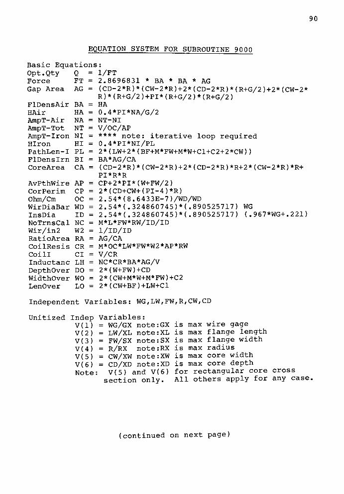
90
EQUATION SYSTEM FOR SUBROUTINE 9000
Basic Equations
Opt.Qty Q =
Force FT =
Gap Area AG =
FlDensAir BA =
HAir HA =
AmpT-Air NA =
AmpT-Tot NT =
AmpT-Iron NI =
HIron HI =
PathLen-I PL =
FlDensIrn BI =
CoreArea CA =
AvPthWire AP =
CorPerim CP =
Ohm/Cm OC =
WirDiaBar WD =
InsDia ID =
NoTrnsCal NC =
Wir/in2 W2 =
RatioArea RA =
CoilResis CR =
Coill CI =
Inductanc LH =
DepthOver DO =
WidthOver WO =
LenOver LO =
1/FT
2.8696831 * BA * BA * AG
(CD-2*R)*(CW-2*R)+2*(CD-2*R)*(R+G/2)+2*(CW-2*
R ) * ( R+G/2 ) +PI * (R+G/2 ) * (R+G/2 )HA
0.4*PI*NA/G/2
NT-NI
V/OC/AP
****note: iterative loop required
0.4*PI*NI/PL
2*(LW+2*(BF+M*FW+M*W+C1+C2+2*CW) )
BA*AG/CA
(CD-2*R)*(CW-2*R)+2*(CD-2*R)*R+2*(CW-2*R)*R+
PI*R*R
CP+2*PI*(W+FW/2)
2*(CD+CW+(PI-4)*R)
2.54*(8.6433E-7)/WD/WD
2. 54* (. 324860745)* ( .890525717) WG
2. 54* ( (.89 0525717) ( . 967*WG+. 221 )
M*L*FW*RW/ID/ID
1/ID/ID
AG/CA
M*OC*LW*FW*W2*AP*RW
V/CR
NC*CR*BA*AG/V
2*(W+FW)+CD
2* (CW+M*W+M*FW)+C2
2*(CW+BF)+LW+C1
Independent Variables: WG,LW,FW,R,CW,CD
Unitized Indep Variables:
V(l) = WG/GX note:GX is max wire gage
V(2) = LW/XL note:XL is max flange length
V(3) = FW/SX note:SX is max flange width
V(4) = R/RX note:RX is max radius
V(5) = CW/XW note:XW is max core width
V(6) = CD/XD note:XD is max core depth
Note: V(5) and V(6) for rectangular core cross
section only. All others apply for any case.
(continued on next page)
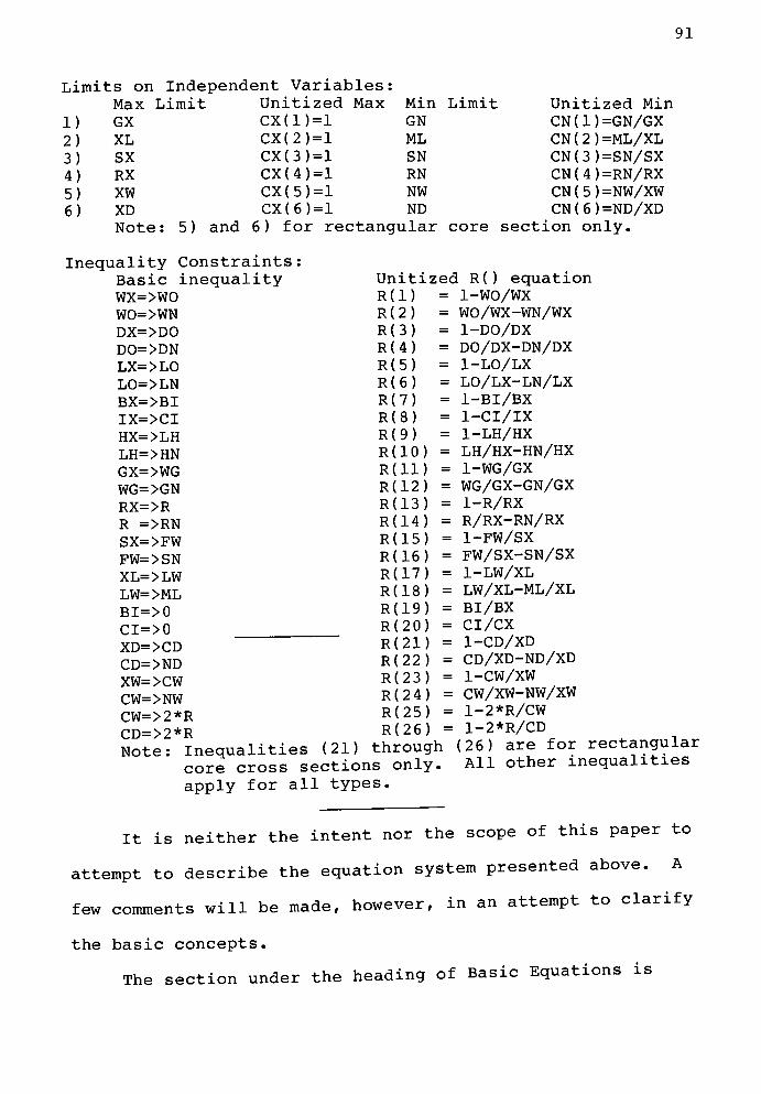
91
Limits on Independent Variables:
Max Limit Unitized Max Min Limit Unitized Min
1) GX CX(1) == 1 GN CN ( 1 ) =GN/GX
2) XL CX(2) ==1 ML CN(2)=ML/XL
3) SX CX(3) == 1 SN CN(3)=SN/SX
4) RX CX(4) ==1 RN CN ( 4 ) =RN/RX
5) XW CX(5) == 1 NW CN ( 5 ) =NW/XW
6) XD CX(6) == 1 ND CN ( 6 ) =ND/XD
Note: 5) and 6) for rectangular core section only.
Inequality Constraints:
Basic inequality Unitized R( ) equation
WX=>WO R(l) = 1-WO/WX
WO=>WN R(2) = WO/WX-WN/WX
DX=>DO R(3) = 1-DO/DX
DO=>DN R(4) = DO/DX-DN/DX
LX=>LO R(5) = 1-LO/LX
LO=>LN R(6) = LO/LX-LN/LX
BX=>BI R(7) = 1-BI/BX
IX=>CI R(8) = 1-CI/IX
HX=>LH R(9) = 1-LH/HX
LH=>HN R(10) = LH/HX-HN/HX
GX=>WG R(1D = 1-WG/GX
WG=>GN R(12) = WG/GX-GN/GX
RX=>R R(13) = 1-R/RX
R =>RN R(14) = R/RX-RN/RX
SX=>FW R(15) = 1-FW/SX
FW=>SN R(16) = FW/SX-SN/SX
XL=>LW R(17) = 1-LW/XL
LW=>ML R(18) = LW/XL-ML/XL
BI=>0 R(19) = BI/BX
CI=>0
XD=>CD
R(20)
R(21)
= CI/CX
= 1-CD/XD
CD=>ND R(22) = CD/XD-ND/XD
XW=>CW R(23) = 1-CW/XW
CW=>NW R(24) = CW/XW-NW/XW
CW=>2*R R(25) = 1-2*R/CW
CD=>2*R R(26) = 1-2*R/CD
Note: Inequalities (21) through (26) are for rectangular
core cross sections only. All other inequalities
apply for all.types.
It is neither the intent nor the scope of this paper to
attempt to describe the equation system presented above. A
few comments will be made, however, in an attempt to clarify
the basic concepts.
The section under the heading of Basic Equations is
92
simply a restatement of equations presented in Chapter II,
and also used in the ANALYSIS program module. The only
additional equation is that for the optimisation quantity, Q,
which has already been discussed.
The next two sections of the preceding equation system
apply to the independent variables. The independent
variables, V(), are the items which the program will vary
during the search process in an attempt to find the lowest
value of Q. The final section in the preceding equation
system summarizes the inequality constraints and the
corresponding functions for the R()*s previously discussed.
All independent variables and inequality constraints
must be unitized. The basic reason for this is to cause all
of the independent variables and the inequality constraints
to carry equal weight. The greater the order of magnitude
difference between the various independent variables, the
greater the importance of scaling becomes. To scale the
independent variables, they are divided by the maximum value
allowed. Then the unitized independent variables, V(), have
an upper limit of one, and a lower limit of no less than
zero. In the event that only a lower limit is present,
unitization is handled differently. Since that does not
occur in this equation system, it will not be discussed.
Finally, the regional constraints are scaled by making
the varying component of the R( ) equations, in each case
between zero and unity, when the inequality constraint is on

93
the verge of violation during the search process.
10.3 Notable Problems
Several unique problems present themselves in the
preceding equation system. When the P519RE program is
normally used, it is set up for one set of conditions. For
the problem being considered in this project, that is not
true. There are four different bobbin configurations, each
of which results in a variant of the equation system.
A method had to be developed, therefore, which would allow
one version of the COIL DESIGN module to be used for all
possible conditions. The alternative would be to have a
different design module for every possible bobbin type.
Aside from the fact that the program occupies 81 disk
sectors, which would fill a disk with less than 7 variations,
there are a large number of possible combinations. For
starters, there are the four basic bobbin types. Within
those, any one or combination of variables could be set to a
fixed value. A variant for each of those possibilities would
be required. It can be seen that this would quickly get out
of hand.
The solution is to arrange the variables in such a way
that the first several are common to all bobbin types. There
is then a branch to any remaining variables. The inequality
constraints and variable limits can be arranged in a similar
manner. Using the bobbin type, the program can determine how
94
many variables, constraints and inequalities to look for, and
where to branch when required.
For variables set to a fixed value, upper and lower
limits can usually be set an arbitrarily small distance
apart and, thereby, essentially hold the variable fixed. The
first problem with this is that the arbitrary value must be
chosen. More important, for each basepoint during the search
process, the program must return to subroutine 9000 twice for
each variable. This is done to determine the effects on the
optimization quantity of changes in each of the variables.
Because of the length of time to execute this program, extra
excursions to subroutine 9000 must be avoided. An invariant
"variable"
would cause two such excursions per basepoint.
To circumvent this problem, and simultaneously avoid
multiple versions of COIL DESIGN, a solution has been found.
Referring to the program listing in Appendix F, line number
4015 has been added. CD(I), is a measure of the difference
between the upper and lower unitized limits for each
variable, V(I). For any of these that are equal to zero, the
program will set the gradient contribution for that variable
equal to zero, and then go to the next variable. Normally,
lines 4020 through 4070, would add and subtract finite
difference increments, CD(I) to and from V(I), and go to
subroutine 9000, for each case. With this approach, only the
active elements of the gradient vector, GB(I), are calculated
for each actual independent variable.
95
The next problem requires some more explanation. An
appropriate penalty function tuning parameter, CP, must be
estimated for the search process of automated optimal design.
The value for CP, must create a proper balance between
penalty function P, and optimization quantity Q, to assure
proper movement in the search process. In addition, penalty
function P, is periodically strengthened as the search
process approaches the solution point, by successively
increasing a factor FP, in the calculation of P.
As previously explained, penalty function P, is added to
the optimization quantity Q, to form a penalized optimization
quantity, X. It is X, which is minimized by the automated
optimal design search process of the program. The search
process continues from basepoint to basepoint, decreasing X,
in each case, until the minimum value of X is found. At this
point, some or all of the constraints may be violated. The
constraint walls of penalty function P, are then steepened,
by increasing FP by a factor of 8. The process is repeated,
until a new minimum is found for X, and then FP is multiplied
by 8 again, and so on. Eventually, the value of FP becomes
so large that if incompatible specifications do not exist,
the optimum design solution point is approximately located,
which meets the design limits. One of the many advantages of
this method is that by allowingexcursions beyond the
feasible design space, answers are obtained even when
incompatible specifications exist, which gives the designer
96
an idea of which limits are active.
One of the drawbacks is that when an equation system has
an unconstrained minimum, which is far removed from the
feasible design space, the initial excursion with FP equal to
unity can be great. It can then take many basepoints and FP
increases to bring the search back within the design bounds.
This is especially true if the optimizing function in Q is
steep enough to overpower the penalty function, FP. The
degree of this problem is also affected by the quality of the
starting point. The closer the start point is to the final
solution, the less severe the problem is likely to be.
This difficulty was encountered with the first runs of
the program. Several hours and over two hundred base points
were required to make the excursion to the first minimum and
then return to the neighborhood of feasible designs. The
answers so derived are correct, but the time factor is
unacceptable .
Because the program is supposed to be user friendly, it
would not be within the rules to ask the user to define a
starting point, and therefore, a built in shotgun routine is
used for this purpose. This routine sprays the n-dimensional
design space of the independent variables with randomly
selected points, to find the lowest value for Q to start the
search from. Theoretically, with enough such trials, the
best design can be found. The time required would be large,
however, to guarantee that the solution found was even close
97
to the best. Therefore, an upper limit must be placed on the
number of shotgun trials allowed before the conjugate
gradient search process is begun.
In the interest of time, a risky solution has been
tried. The answers obtained agree with the several full time
runs made with the same constraints, and are consistent with
other runs made with slightly different constraints and
bobbin types. During the shotgun routine in subroutine 2 000,
some lines of code have been added. Initially, FP is set to
262144 in line 57. The normal shotgun search proceeds until
the minimum number of trials, MN, is reached. For the
example, MN is equal to 50. If the penalty function P, is
zero for the design of lowest X, then that basepoint is
accepted as a starting point and FP, is retained. If not,
the search continues until a P of zero is found or the
maximum number of points, MX, is reached. For this example,
MX is equal to 100.
If no starting point has been found, which falls within
the feasible design space, then FP, is reduced by a factor of
eight, and the process repeated. In the worst case, a
situation will arise where FP gets back to unity, as in the
unmodified program, without finding a start point meeting all
constraints, as defined by a P of zero. There are two
dangers to this solution.
The first is that the tuning parameter, CP, is
determined by the steps from the start point. If CP is
98
poorly set, it is very possible that a situation will arise
where either no motion will occur about a basepoint causing
the program to apparently hang or the program will
prematurely decide that the best solution has been found.
This could happen when the start point is actually very far
removed from the actual solution point. It is less likely to
occur as the initial start point gets closer to the solution
point. The highest number of shotgun trials is desired,
therefore, while still keeping the time to a reasonable
level.
The second potential problem requires a trip into n-
dimensional space. Since that is difficult to imagine, the
example will be limited to three dimensions. Think of a
curved trough winding its way around a mountain in a
gradually descending direction. Eventually, this trough
leads to the best solution. It is entirely possible that the
curve of the trough could extend beyond an imaginary vertical
limit wall during its curved descent before coming back
through the wall into the acceptable space domain. If the
limit function is too steep, the descent will stop where the
wall and trough meet, even though there is a better solution
on the other side of the mountain which could be reached if
the limit were shallower.
Without a lot of trials using many different
configurations and limits, it is almost impossible to
determine if this last problem exists. Again, the best
99
solution is to spend more time during the initial shotgun
search trying to find a spot in the trough on the correct
side of the mountain.
One way to check a solution is to repeat the design
process. If the same solution is found, the chances are good
that the global optimization solution point has been reached.
If another solution with the same value of Q, is found, but
different values for the independent variables, a region
containing a range of equivalent designs has probably been
found, and any solution between these two solutions will
likely give the same answer for force. Again, the best
solution has been found. If, however, a different value of Q
has been found at the end of the searches, then a problem has
been encountered in the automated optimal design search
process. The solution is to set FP to unity in line 57, as
in the original form, and wait for the design process to end.
Occasional checks of solutions, using FP equal to one, are
advised until a better base can be established to prove or
disprove the validity of the change described.
For the designs tested, no problems occurred and,
therefore, the code has been left in the shotgun subroutine.
In the event that a set of design constraints exist, which do
not yield a start point with an initial value of zero for the
penalty function P, then the approach presented will reduce
the initial value of FP, to unity. Since this is equivalent
to the unmodified program, and since the option exists for
100
setting FP, to unity in line 57, the extra code can do no
harm. The benefit of the extra code is that it successfully
found the same solution as the originally intended method in
approximately one fifth the number of basepoints, and thus
one fifth the amount of time.
10.4 Programming Notes
This program was converted from an original version
available in the TRS-80 Basic language. Two modifications
have been made. The first, was to remove the double
precision calculations, since they are not available on the
Apple 11+ microcomputer. The second, was to add an
occasional A=FRE(0) command at strategic locations as a
housecleaning measure, which is compatible with an Apple
microcomputer. If transferred to another system, the
original version should be restored. Other than this, no
special system dependent commands exist.
CHAPTER XI
SAMPLE COMPUTER TRIALS AND OBSERVATIONS
11.1 Introduction
The aim of this chapter will be to demonstrate the
effectiveness of the design process developed for this
project. To do this, a commercially produced electromagnet
of the general size being considered has been found and
measured. Its outside dimensions, operating voltage and
current are shown in Figure 12, and appear as maximum limits.
These will then become the design constraints for the trials
which follow.
In addition to an analysis of the production design,
which is identical to that presented in Chapter II, there are
five input configurations given for the trials. They have
been chosen for two basic reasons. The first is to determine
which of the four core shape and bobbin combinations shown in
Figure 9, gives the maximum holding force permitted by the
design constraints. The second is to provide a thorough
check of the equation variations in each of the program
modules dictated by these coil varieties.
To satisfy this second purpose, a fifth trial is needed.
When executing the designs for the rectangular bobbins, a
maximum core corner radius of zero is specified to insure
rectangular core cross sections. The fifth run is a
101
102
variation on this cross section which sets the maximum corner
radius equal to half of the maximum core width or depth.
This checks the inequality constraint equations of the COIL
DESIGN module, which require that the corner radii be less
than half of the smallest core dimension. If this condition
is violated, some of the equations in the equation system
become invalid.
11.2 Sample Runs
Figures 12 through 35, on the next 24 pages, show the
summary pages for the five runs being considered. The
intermediate results for the design phases are not included
to reduce the output to a reasonable level. The highlights
of those results will be discussed in section 11.3.
For each of the five trial examples, there are four
figures. The first one is the drawing of the design
requirements, which were used as the inputs to the COIL
DESIGN module. For each of the five examples, the maximum
and minimum outside dimensions, overall core limits, wire
size limits, and electrical requirements are identical. In
addition, those factors, which are set by the manufacturing
limitations, CI, C2, BF, W, RW and V, are the same. Core
material and an assumed air gap are likewise equal. The only
difference between the two single bobbin, rectangular core
runs, is that the last one allows the corner radii to take on
a value different from zero.
103
The second figure in each group is a drawing of the
optimum design found by the COIL DESIGN module. Included on
these drawings are all of those dimensions and inputs
necessary for manufacturing a sample of the design. Special
features, such as mounting tabs, are left to the designer,
since they do not affect the magnetic or electrical
characteristics of the coil. In addition, the assumption is
made that adequate clearance has been allowed for, in
dimension C2, and the overall width and depth, to increase
the bobbin flange widths. This is to allow for the
deficiencies in equation (1), discussed in section 2.2.
The third figure is the graph and a partial listing from
the sensitivity study. It shows the no-loss holding force as
a function of operating voltage for three different air gaps.
In each case, the voltage range is from zero to 6.5 volts,
and the arbitrary air gaps chosen are 0.0015, 0.003 and
0.0045 centimeters. The point indicated by 3 volts on the
0.0015cm air gap curve is the design point for each of the
coils. Had the design requirements been different, the final
design and thus these curves would also be different. The
objective of the sensitivity study is to show the designer
how the coil will behave under conditions varying slightly
from the single design point.
Normally, the full output of the sensitivity study would
show the voltage and force used to generate the graph for
each of the airgaps considered. For brevity, only the
104
information for the designed air gap is shown.
The final"figure"
is the full listing from the ANALYSIS
program module. It shows not only the analysis of the
expected performance of the device, but also the input
requirements to, and the specified dimensions from, the COIL
DESIGN module. The first example, labeled "Production
Design"
shows design constraints, even though the design was
not subjected to the optimization program. These dimensions
have been placed in the listing for reference. With the
exception of the maximum core width and depth dimensions,
these design constraints should match the actual dimensions.
The reader should take more than a brief look at these
figures before continuing to section 11.3, where they will be
discussed in detail. This will make the discussions in that
section more meaningful.
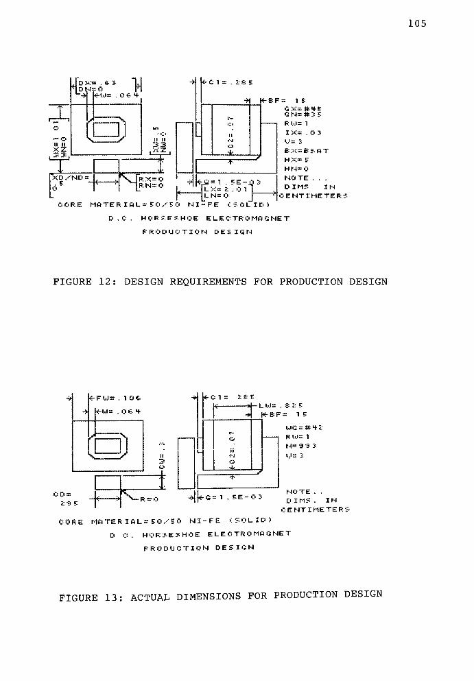
105
1DN=0 n--d frW=
. O 6- +
4-C1
-M K-bf = i s
XD /ND :
. 5O
\Jrx=o^-{rn=o
fL X=. O 1 |
|ln=oJ-
G X= # f SCiN=#3
R W= 1
I X= . O 3
BX=BSST
H X= 5
HN=0
NOTE . . .
DIMS I N
CENT IMETE P. -J
CORE MfiTER I ft L = SO/50 NI-FE (SOLID)
D.C. HORSESHOE E L E C TR O Mfi GNE T
P P. O D U C T I O N DESION
FIGURE 12: DESIGN REQUIREMENTS FOR PRODUCTION DESIGN
* FW=. 1 O 6
<H-.<=. O = f
CD:
-*<- C 1 = 2 S E
l_ W=. S E E
K-EF= 1 5
WG = ttH-E
R w= 1
N= -3 3 3
f*- G = 1 . E E - O 2=NOTE . .
D I MS . I N
CENTIMETER:
CORE MfiTERIftL= SO,--50 NI-FE (SOLID)
D C .HORSESHOE E L E C TR O Mft GNE T
PRODUCTION DESIGN
FIGURE 13: ACTUAL DIMENSIONS FOR PRODUCTION DESIGN

106
Ui
o
u.
MO LTOOE
UOLTAGE AND AIRGAP SENSITIOITV FOR PRODUCTION DESIGN
GAP UOLTAGE
1 . 5E-Q3 .5
1 . 5E-03 1
1 . 5E-03 1.5
1 . 5E-63 xL
1 . 5E-83 2.5
1 . 5E-S3 3
1 . 5E-83 3.5
1 . 5E-03 4
1 . 5E-Q3 4.5
1 . 5E-03 5
1 . 5E-03 5.5
1 . 5E-03 6
1 . 5E-03 6.5
IDEAL FORCE<OZ3)
1.06137541
3.81817831
9.8993974
17.7141935
26.7335985
35.6110349
39 . 0402587
42.8103483
45.9421093
46.3639406
46.7963059
47.2363749
FIGURE 14: GAP AND VOLTAGE SENSITIVITY FOR PRODUCTION DESIGN
WITH LISTING FOR FIRST GAP ONLY

107
SAMPLE RUN FOR A SINGLE BOBBIN, RECTANGULAR CORE
SUBJECT TO THE STANDARD LIMITS OF THIS PROJECT
COIL NAME PRODUCTION DESIGN
COIL TYPE: SINGLE BOBBIN, RECTANGULAR CORE
OPERATING VOLTAGE: 3
COIL RESISTANCE: 97. 3121734
CORE MATERIAL: 50/50 NI-FE (SOLID)
THEORETICAL, NO LOSS HOLDING FORCE(OZ ): 35. 6110349
EXPECTED HOLDING FORCE (OZ):22. 7910623
****PHYSICAL DIMENSIONS & CONSTANTS****
OVERALL LENGTH: 2. 01
OVERALL DEPTH : . 6 3 5
OVERALL WIDTH: 1.01
FLANGE WIDTH: .106
WINDING LENGTH:. 825
BOBBIN WALL THICKNESS :. 064
BOBBIN FLANGE THICKNESS :. 15
ARMATURE/BOBBIN CLEARANCE : . 2 8 5
WINDING CLEARANCE: . 07
AIRGAP :1.5E- 03
STEEL PATH LENGTH: 4. 5
CORE WIDTH:. 3
CORE DEPTH: .295
CORNER RADIUS :0
CORE PERIMETER: 1.19
CORE AREA:. 0885
AIRGAP AREA (FRINGING) :. 0893942672
WINDING SURFACE AREA: 1. 6414 5992
************* *WINDING DATA* *************
WIRE GAGE NUMBER: #42
TURNS SPECIFIED: 993
TURNS POSSIBLE: 1663. 68481
RANDOM WIND:1
WINDING WIDTH: .0632679935
BARE WIRE DIA:6.33406496E-03
OHMS/CM OF WIRE:. 0547204868
EFFECTIVE INSUL.WG : 40 . 835
INSULATED WIRE DIA: 7 .25010641E-03
THEORETICAL TURNS/SQ CM=19024 . 4118
CURRENT AT 3 VOLTS :. 0308286199
AVERAGE TURN LENGTH: 1 .79088612
INDUCTANCE, HENRIES:. 33 9 2 54 27 4
S.S.TEMP RISE, DEG C:56. 819184
FIGURE 15: ANALYSIS LISTING FOR PRODUCTION DESIGN
(CONTINUED ON NEXT PAGE)
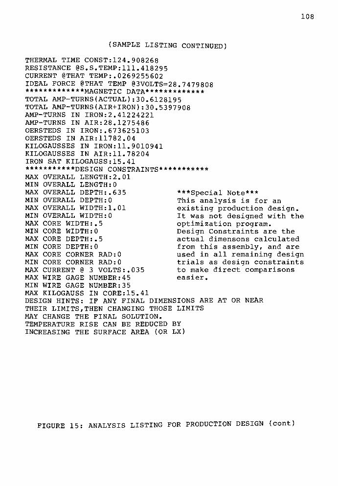
108
(SAMPLE LISTING CONTINUED)
THERMAL TIME CONST: 124 . 908268
RESISTANCE @S. S. TEMP : 111 . 418295
CURRENT @THAT TEMP :. 0269255602
IDEAL FORCE @THAT TEMP 3VOLTS=28 . 747 9808************ *MAGNETIC DATA*************
TOTAL AMP-TURNS (ACTUAL ):30. 6128195TOTAL AMP-TURNS (AIR+IRON) :30. 5397908AMP-TURNS IN IRON: 2 . 41224221
AMP-TURNS IN AIR: 28 . 1275486
OERSTEDS IN IRON: . 673625103
OERSTEDS IN AIR: 11782. 04
KILOGAUSSES IN IRON: 11. 9010941
KILOGAUSSES IN AIR: 11. 78204
IRON SAT KILOGAUSS:15.41
********* * *DES IGN CONSTRAINTS***********
MAX OVERALL LENGTH: 2. 01
MIN OVERALL LENGTH :0
MAX OVERALL DEPTH:. 635
MIN OVERALL DEPTH :0
01MAX OVERALL WIDTH :1
MIN OVERALL WIDTH :0
MAX CORE WIDTH : . 5
MIN CORE WIDTH :0
MAX CORE DEPTH: .5
MIN CORE DEPTH :0
MAX CORE CORNER RAD : 0
MIN CORE CORNER RAD : 0
MAX CURRENT @ 3 VOLTS:. 03 5
MAX WIRE GAGE NUMBER: 45
MIN WIRE GAGE NUMBER: 35
MAX KILOGAUSS IN CORE: 15. 41
DESIGN HINTS: IF ANY FINAL DIMENSIONS ARE AT OR NEAR
THEIR LIMITS, THEN CHANGING THOSE LIMITS
MAY CHANGE THE FINAL SOLUTION.
TEMPERATURE RISE CAN BE REDUCED BY
INCREASING THE SURFACE AREA (OR LX)
***Special Note***
This analysis is for an
existing production design.
It was not designed with the
optimization program.
Design Constraints are the
actual dimensons calculated
from this assembly, and are
used in all remaining design
trials as design constraints
to make direct comparisons
easier.
FIGURE 15: ANALYSIS LISTING FOR PRODUCTION DESIGN (cont)
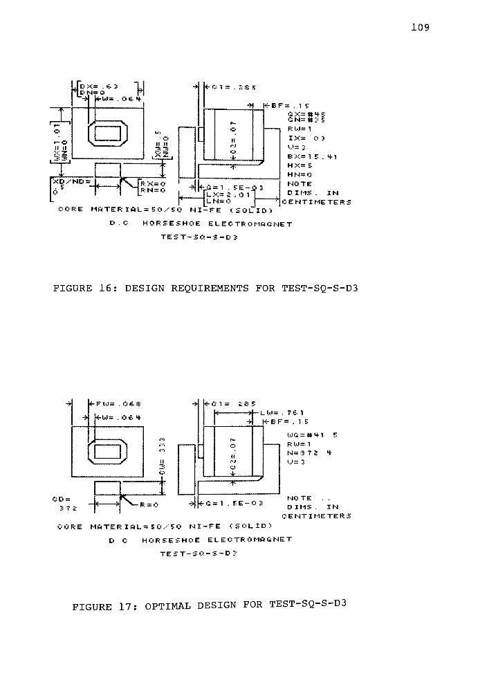
109
m
xr-O
II II
xz
DN=0 "H06- +
I
S
XD.--ND =
. 5O
33
. XZ
RRX=0ft N= O
- (-C1:
hrBF=. 1 E
k-G= 1 . EE-o;
JLX= 2 .Oil
|ln=oJ"
CNs*3 5
RW= 1
I X= 0 3
','= 3
B X= 1 E . H 1
H X= E
HN=0
NOTE
D I MS . I N
CENTIMETERS
CORE MATER IAL= EC'S O NI-FE (SOLID)
D.C HORSESHOE E 1_ E O TR OMft GNE T
TEST-SCl -3-D 3
FIGURE 16: DESIGN REQUIREMENTS FOR TEST-SQ-S-D3
<r FW=. O 6 S
rw=. o e- +
=U
CD =
3 T 2>^IR = C
-HH- c i = "s
=-
-LW=. T 1
tf-BF = . 1 E
WG = # + 1
RW= 1
N= 3 7 2
V= 3
k< 1 . E E - O 3NOTE
D IMS IN
CENTIMETERS
CORE MATER IAL= SO,-SO NI-FE (SOLID)
D C HORSESHOE ELECTROMAGNET
TE ST-SC'
- S - D 3
FIGURE 17: OPTIMAL DESIGN FOR TEST-SQ-S-D3

110
Ul
o
a
Q
W'LTSSE
UOLTAGE AND AIRGAP SENSITIUITV FOR TEST- 5Q-S-D3
GAP
1 . 5E-03
1 . 5E-03
1 . 5E-03
1 . 5E-03
1 . 5E-03
1 . 5E-03
1 . 5E-03
1 . 5E-03
1 . 5E-03
1 . 5E-03
1 . 5E-03
1 . 5E-03
1 . 5E-03
UOLTAGE
1 SJ-
4.5
6.5
IDEAL FORCEC02
1.47317379
5.30115315
13.7150375
24.5712921
37. 0978613
49.5609966
54.5932249
59.9166149
64 . 3093856
64 . 9074733
65.520768
66. 1451627
fc>6. 7783338
FIGURE 18: GAP AND VOLTAGE SENSITIVITY FOR TEST-SQ-S-D3
WITH LISTING FOR FIRST GAP ONLY

Ill
SAMPLE RUN FOR A SINGLE BOBBIN, RECTANGULAR CORE
SUBJECT TO THE STANDARD LIMITS OF THIS PROJECT
COIL NAME:TEST-SQ-S-D3
COIL TYPE: SINGLE BOBBIN, RECTANGULAR CORE
OPERATING VOLTAGE: 3
COIL RESISTANCE: 85. 7314358
CORE MATERIAL: 50/50 NI-FE (SOLID)
THEORETICAL, NO LOSS HOLDING FORCE ( OZ ): 49 . 5609966
EXPECTED HOLDING FORCE (OZ ): 31 . 7190378
****PHYSICAL DIMENSIONS & CONSTANTS****
OVERALL LENGTH: 2. 01084969
OVERALL DEPTH:. 635156443
OVERALL WIDTH:. 998625621
FLANGE WIDTH: .0676721706
WINDING LENGTH: .76056841
BOBBIN WALL THICKNESS :. 064
BOBBIN FLANGE THICKNESS :. 15
ARMATURE/BOBBIN CLEARANCE : . 2 8 5
WINDING CLEARANCE:. 07
AIRGAP :1.5E- 03
STEEL PATH LENGTH: 4 . 42504373
CORE WIDTH:. 33264064
CORE DEPTH:. 371812102
CORNER RADIUS :0
CORE PERIMETER: 1.40890548
CORE AREA:. 123679816
AIRGAP AREA( FRINGING) : .124738262
WINDING SURFACE AREA: 1. 70080295
************* *WINDING DATA* *************
WIRE GAGE NUMBER: #41. 4850841
TURNS SPECIFIED:872. 399078
TURNS POSSIBLE: 872. 399069
RANDOM WIND:1
WINDING WIDTH: .0676721706
BARE WIRE DIA:6.7237313E-03
OHMS/CM OF WIRE:. 0485617446
EFFECTIVE INSUL.WG : 40 . 3370763
INSULATED WIRE DIA: 7 .68097937E-03
THEORETICAL TURNS/SQ CM=16949 . 8868
CURRENT AT 3 VOLTS :. 0349929985
AVERAGE TURN LENGTH: 2 . 023 62774
INDUCTANCE , HENRIES : . 365920659
S.S.TEMP RISE, DEG C:61. 2650785
FIGURE 19: ANALYSIS LISTING FOR TEST-SQ-S-D3
(CONTINUED ON NEXT PAGE)

112
(SAMPLE LISTING CONTINUED)
THERMAL TIME CONST: 132 . 207211
RESISTANCE @S. S. TEMP : 99 . 6594453
CURRENT @THAT TEMP :. 0301025155
IDEAL FORCE @THAT TEMP 3VOLTS=3 9 . 3710353
*************MAGNETIC DATA*************
TOTAL AMP-TURNS (ACTUAL) :30. 5278593
TOTAL AMP-TURNS (AIR+IRON) :30. 4312144
AMP-TURNS IN IRON: 2 . 34038302
AMP-TURNS IN AIR: 28 . 0908313
OERSTEDS IN IRON: . 664628922
OERSTEDS IN AIR: 11766 . 6599
KILOGAUSSES IN IRON: 11 . 8673585
KILOGAUSSES IN AIR: 11. 7666599
IRON SAT KILOGAUSS:15.41
***********DESIGN CONSTRAINTS***********
MAX OVERALL LENGTH: 2. 01
MIN OVERALL LENGTH :0
MAX OVERALL DEPTH:. 635
MIN OVERALL DEPTH :0
MAX OVERALL WIDTH: 1.01
MIN OVERALL WIDTH :0
MAX CORE WIDTH: .5
MIN CORE WIDTH :0
MAX CORE DEPTH: .5
MIN CORE DEPTH :0
MAX CORE CORNER RAD : 0
MIN CORE CORNER RAD : 0
MAX CURRENT @ 3 VOLTS:. 03 5
MAX WIRE GAGE NUMBER: 45
MIN WIRE GAGE NUMBER: 35
MAX KILOGAUSS IN CORE: 15. 41
DESIGN HINTS:
IF ANY FINAL DIMENSIONS ARE AT OR NEAR
THEIR LIMITS, THEN CHANGING THOSE LIMITS
MAY CHANGE THE FINAL SOLUTION.
TEMPERATURE RISE CAN BE REDUCED BY
INCREASING THE SURFACE AREA (OR LX)
FIGURE 19: ANALYSIS LISTING FOR TEST-SQ-S-D3 (cont)

113
Jo x= . e s 1J*1dn=o n"-* hrW=
. O = t
o
-o
II II
XZ
((")) I
I I
II II
XZ
-><- C 1 = 2 S E
fi-BF
O
IIJ
o
+J
-1 ft*|L
= 1 . EE-.<= 2 . o i
?::
LLI
G X= # t SG N= * 3 E
RW= 1
IX=. O 3
'.'= 3
BX= IE ."i
H X= E
HN= O
NOTE . .
DIMS IN
CENTIMETERS
CORE MATER IAL= 50/ SO NI-FE (SOL ID J
D . C HORSESHOE E L E C TR 0 MA G NE T
TEST-RND-S-D +
FIGURE 20: DESIGN REQUIREMENTS FOR TEST-RND-S-D4
<- F 1.0= O E &
4
C 1
LW= T 3 2
K-BF= IE
k G= 1
CORE MATER IAL= EO/S(
D.C.
WG = # M- Z
R W= 1
N= 3 7 3
NOTE . .
D IMS . I N
CENTIMETER:
NI-FE (SOLID)
HORSESHOE E L E C TR O MO GNE T
TEST-RNO-S-Dt
FIGURE 21: OPTIMAL DESIGN FOR TEST-RND-S-D4

114
o
MO L TO G E
UOLTAGE AND AIRGAP SENS
GAP UOLTAGE
1 . 5E-03 .5
1 . 5E-03 1
1 . 5E-03 1.5
1 . 5E-03 xi
1 . 5E-03 2.5
1 . 5E-03 .$
1 . 5E-03 3.5
1 . 5E-03 4
1 . 5E-03 4.5
1 . 5E-03 5
1 . 5E-03 5.5
1 . 5E-03 6
1 . 5E-03 6.5
FOR TEST-RND-S-D4
IDEAL FORCE <OZ>
1.141 03006
4 . 09988428
10.6444263
19
28.
TOs-'O -
41.
45.
49.
49.
50.
50.
50.
, 03583 1 2
, 7555072
,3173211
,8169219
, 9555203
, 0667859
, 52868 1 9
0021145
4840864
9726 1 2
FIGURE 22: GAP AND VOLTAGE SENSITIVITY FOR TEST-RND-S-D4
WITH LISTING FOR FIRST GAP ONLY
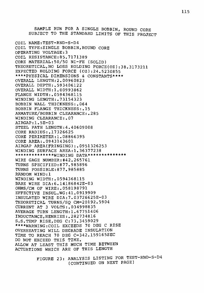
115
SAMPLE RUN FOR A SINGLE BOBBIN, ROUND CORE
SUBJECT TO THE STANDARD LIMITS OF THIS PROJECT
COIL NAME:TEST-RND-S-D4
COIL TYPE: SINGLE BOBBIN, ROUND CORE
OPERATING VOLTAGE: 3
COIL RESISTANCE: 85. 7171389
CORE MATERIAL: 50/50 NI-FE (SOLID)
THEORETICAL, NO LOSS HOLDING FORCE(OZ ): 38 . 3173211
EXPECTED HOLDING FORCE (OZ ): 24 . 5230855
****PHYSICAL DIMENSIONS & CONSTANTS****
OVERALL LENGTH: 2. 00960823
OVERALL DEPTH:. 593406122
OVERALL WIDTH: 1.00993862
FLANGE WIDTH:. 0594368115
WINDING LENGTH:. 73154323
BOBBIN WALL THICKNESS :. 064
BOBBIN FLANGE THICKNESS :. 15
ARMATURE/BOBBIN CLEARANCE : . 2 8 5
WINDING CLEARANCE : . 07
AIRGAP :1.5E- 03
STEEL PATH LENGTH: 4 . 40609008
CORE RADIUS: .17326625
CORE PERIMETER: 1. 08866395
CORE AREA:. 0943143601
AIRGAP AREA (FRINGING) :. 0951326253
WINDING SURFACE AREA: 1 . 36377238
************* *WINDING DATA* *************
WIRE GAGE NUMBER: #42. 265761
TURNS SPECIFIED: 877. 985896
TURNS POSSIBLE:877. 985885
RANDOM WIND:1
WINDING WIDTH:. 0594368115
BARE WIRE DIA:6.14186842E-03
OHMS/CM OF WIRE:. 058198791
EFFECTIVE INSUL.WG : 41 . 0919909
INSULATED WIRE DIA: 7 . 03726625E-03
THEORETICAL TURNS/SQ CM=20192 . 59 04
CURRENT AT 3 VOLTS :. 034998835
AVERAGE TURN LENGTH: 1 . 67751406
INDUCTANCE, HENRIES:. 282734816
S.S.TEMP RISE, DEG C:73. 3459029
****WARNING:COIL EXCEEDS 70 DEG C RISE
OVERHEATING WILL DEGRADE INSULATION
TIME TO REACH 70 DEG C=342 .159165SEC
DO NOT EXCEED THIS TIME.
ALLOW AT LEAST THIS MUCH TIME BETWEEN
ACTUATIONS WHICH ARE OF THIS LENGTH
FIGURE 23: ANALYSIS LISTING FOR TEST-RND-S-D4
(CONTINUED ON NEXT PAGE)

116
(SAMPLE LISTING CONTINUED)
THERMAL TIME CONST: 110 . 822574
RESISTANCE @70 DEG C:102. 590591
CURRENT @THAT TEMP :. 0292424477
IDEAL FORCE @THAT TEMP @3VOLTS=28 . 94 04781************ *MAGNETIC DATA* ************
TOTAL AMP-TURNS (ACTUAL ):30. 7284831
TOTAL AMP-TURNS (AIR+IRON) :30. 6907342
AMP-TURNS IN IRON : 2 . 40761853
AMP-TURNS IN AIR: 28 . 2831156
OERSTEDS IN IRON :. 686663825
OERSTEDS IN AIR: 11847 . 2038
KILOGAUSSES IN IRON: 11. 9499893
KILOGAUSSES IN AIR: 11. 8472038
IRON SAT KILOGAUSS:15.41
********* * *DESIGN CONSTRAINTS ***********
MAX OVERALL LENGTH: 2. 01
MIN OVERALL LENGTH :0
MAX OVERALL DEPTH:. 635
MIN OVERALL DEPTH :0
MAX OVERALL WIDTH: 1.01
MIN OVERALL WIDTH :0
MAX CORE WIDTH:. 5
MIN CORE WIDTH :0
MAX CORE DEPTH:. 5
MIN CORE DEPTH :0
MAX CORE CORNER RAD : . 2 5
MIN CORE CORNER RAD : 0
MAX CURRENT @ 3 VOLTS:. 035
MAX WIRE GAGE NUMBER: 45
MIN WIRE GAGE NUMBER: 35
MAX KILOGAUSS IN CORE: 15. 41
DESIGN HINTS:
IF ANY FINAL DIMENSIONS ARE AT OR NEAR
THEIR LIMITS, THEN CHANGING THOSE LIMITS
MAY CHANGE THE FINAL SOLUTION.
TEMPERATURE RISE CAN BE REDUCED BY
INCREASING THE SURFACE AREA (OR LX)
FIGURE 23: ANALYSIS LISTING FOR TEST-RND-S-D4 (cont)
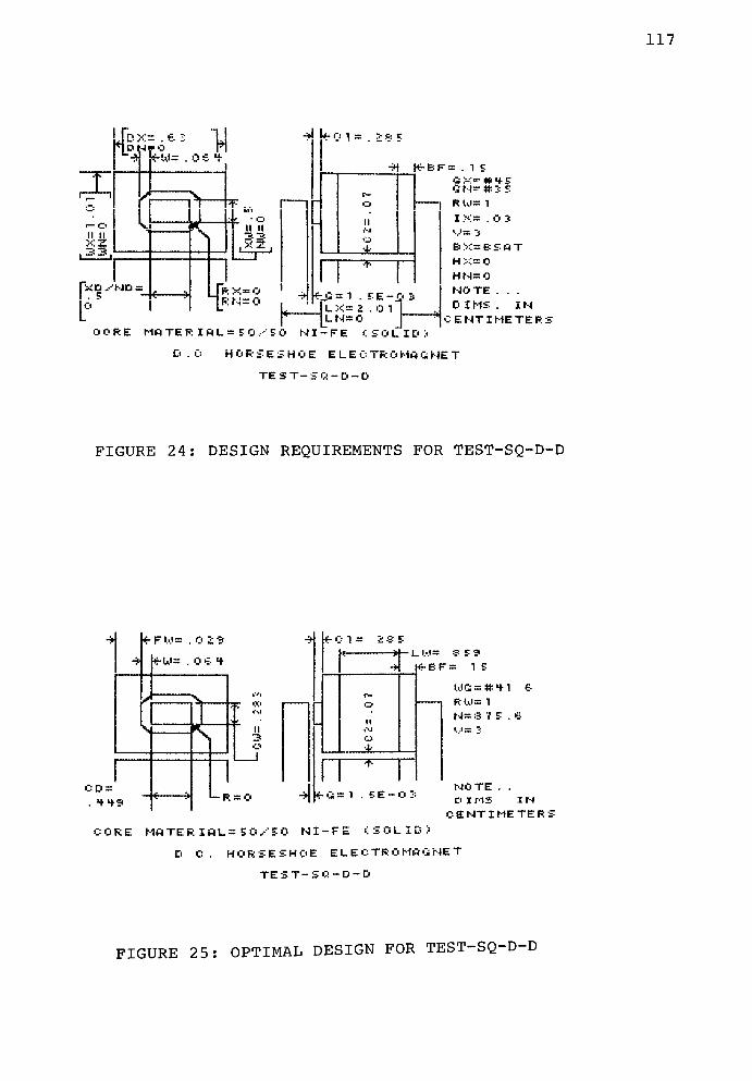
117
.X
i
o
II II
-l-O
irW=. o e 1
r
XD/ND:
"H
>
*r n u
33,XZ
^l_P:N= 0
< 0 1 :
II
-H K-BF=.1S
-G= 1 . FE-C
M_X= 2.01
jLN= O
GM=#3 S
RW= 1
IX=. 0 3
','= 3
BX=BSOT
HX=0
HN= O
NOTE . . .
D IMS. I N
centimeter;
OORE MfiTER IflL= EO,- EO NI-FE (SOLID)
D . 0 HORSESHOE E L E 0 TR 0MA GNE T
TEST-SC! -D-D
FIGURE 24: DESIGN REQUIREMENTS FOR TEST-SQ-D-D
<t-FW=.0 29
*W=. O 6 t
CD =
. tH-3
TT. "
L- ft-
O
-i1 **C : 1 = 2 3 r.
K-BF= 1 E-
,-..,
-
ru.
O
II
im
o
J,
WG = # M- 1 6
RW= 1
N= 3 T E . 61--J
II
3o
H*
IT*-G == 1 .
EE- 0 3NOTE . .
D IMS I N
CENTIMETER
CORE MflTERIflL=EO/SO NI-FE (SOLID)
D C . HORSESHOE ELECTROMAGNET
TEST-SO-D-D
FIGURE 25: OPTIMAL DESIGN FOR TEST-SQ-D-D

118
3 3 -
3 H- -
"
MI
6 0 -
E3 -
E 2 -
Ul
o
4-3 -
-
cc:to -
u. 33-
_l
3 2-
3
Ul
CI
2 3 -
2 H- -
l-l 2 0 -
1 3 -
1 E _
3 -
+ -i
M IN G A R = 1 E E - 0 3
MO L TO G E
UOLTAGE AND AIRGAP SENS
GAP UOLTAGE
1 . 5E-03er
1 . 5E-03 l
1 . 5E-83 1.5
1 . 5E-03 ii
1 . 5E-03 A., w"
1 . 5E-03 yt
1 . 5E-03 3.5
1 . 5E-03 4
1 .5E03 4.5
1 . 5E-03 5
1 . 5E-03 5.5
1 . 5E-03 6
1 . 5E-03
FOR TEST-SQ-D-D
IDEAL F0RCE<0Z3)
1.52509182
5. 48790488
14.224711
25. 4568527
38.4094152
51. 1549686
56. 1343459
61.5206589
66. 1826233
66.7055791
67.3235823
67 . 9525833
68 . 5902854
FIGURE 26: GAP AND VOLTAGE SENSITIVITY FOR TEST-SQ-D-D
WITH LISTING FOR FIRST GAP ONLY

119
SAMPLE RUN FOR A DOUBLE BOBBIN, RECTANGULAR CORE
SUBJECT TO THE STANDARD LIMITS OF THIS PROJECT
COIL NAME: TEST-SQ-D-D
COIL TYPE: DOUBLE BOBBIN, RECTANGULAR CORE
OPERATING VOLTAGE: 3
COIL RESISTANCE: 85. 7189312
CORE MATERIAL: 50/50 NI-FE (SOLID)
THEORETICAL, NO LOSS HOLDING FORCE(OZ ): 51. 1549686
EXPECTED HOLDING FORCE (OZ):32. 7391799
****PHYSICAL DIMENSIONS & CONSTANTS****
OVERALL LENGTH: 2. 0107 306
OVERALL DEPTH:. 63521718
OVERALL WIDTH:1. 00976745
FLANGE WIDTH:. 0292383872
WINDING LENGTH:. 858916697
BOBBIN WALL THICKNESS :. 064
BOBBIN FLANGE THICKNESS :. 15
ARMATURE/BOBBIN CLEARANCE : . 2 8 5
WINDING CLEARANCE : . 07
AIRGAP :1.5E- 03
STEEL PATH LENGTH: 4 . 53441475
CORE WIDTH:. 283406952
CORE DEPTH:. 448740406
CORNER RADIUS :0
CORE PERIMETER: 1.46 429472
CORE AREA: .127176151
AIRGAP AREA ( FRINGING ):. 12 827 613 9
WINDING SURFACE AREA: 3 . 52177968
************* *WINDING DATA* *************
WIRE GAGE NUMBER: #41. 6103187
TURNS SPECIFIED:875. 582503
TURNS POSSIBLE:875. 582495
RANDOM WIND:1
WINDING WIDTH:. 0292383872
BARE WIRE DIA:6.62680734E-03
OHMS/CM OF WIRE: .0499926652
EFFECTIVE INSUL.WG : 40 .4581782
INSULATED WIRE DIA: 7 .57388474E-03
THEORETICAL TURNS/SQ CM=17432 . 6181
CURRENT AT 3 VOLTS :. 0349981032
AVERAGE TURN LENGTH: 1. 95827368
INDUCTANCE,HENRIES:. 37831403
S.S.TEMP RISE, DEG C:32. 9281411
FIGURE 27: ANALYSIS LISTING FOR TEST-SQ-D-D
(CONTINUED ON NEXT PAGE)
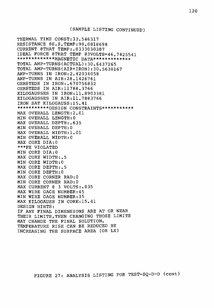
120
(SAMPLE LISTING CONTINUED)
THERMAL TIME CONST: 33 . 546317
RESISTANCE @S. S. TEMP : 90 . 0818698
CURRENT @THAT TEMP :. 0333030387
IDEAL FORCE @THAT TEMP @3VOLTS=46 . 7425541************ *MAGNETIC DATA* ************
TOTAL AMP-TURNS (ACTUAL) :30. 6437265TOTAL AMP-TURNS (AIR+IRON) :30. 5630167AMP-TURNS IN IRON: 2 . 42034058
AMP-TURNS IN AIR: 28 . 1426761
OERSTEDS IN IRON: . 670756832
OERSTEDS IN AIR: 11788. 3766
KILOGAUSSES IN IRON: 11 . 8903381
KILOGAUSSES IN AIR: 11. 7883766
IRON SAT KILOGAUSS:15.41********* * *DES IGN CONSTRAINTS***********
MAX OVERALL LENGTH: 2. 01
MIN OVERALL LENGTH :0
MAX OVERALL DEPTH:. 63 5
MIN OVERALL DEPTH :0
MAX OVERALL WIDTH: 1.01
MIN OVERALL WIDTH :0
MAX CORE DIA:0
***PX VIOLATED
MIN CORE DIA:0
MAX CORE WIDTH: .5
MIN CORE WIDTH :0
MAX CORE DEPTH : . 5
MIN CORE DEPTH :0
MAX CORE CORNER RAD:0
MIN CORE CORNER RAD : 0
MAX CURRENT @ 3 VOLTS:. 035
MAX WIRE GAGE NUMBER: 45
MIN WIRE GAGE NUMBER: 35
MAX KILOGAUSS IN CORE: 15. 41
DESIGN HINTS:
IF ANY FINAL DIMENSIONS ARE AT OR NEAR
THEIR LIMITS, THEN CHANGING THOSE LIMITS
MAY CHANGE THE FINAL SOLUTION.
TEMPERATURE RISE CAN BE REDUCED BY
INCREASING THE SURFACE AREA (OR LX)
FIGURE 27: ANALYSIS LISTING FOR TEST-SQ-D-D (cont)

121
J~D X=. 3 3 "11
*1 DN= O n
r^r
r-O
n ii
xz33.
<rW=
U ).i III II
-C 1 = 2 S E
-H H-BF:
o
. 1 E
^Ji= 1 . PE-Jf 3L X= 2 . O 1
LN= O
GX=#tGN= # 3
RW= 1
I X= . 0 J
V= 3
B X= 1 E
HX= E
HN=0
NOTE .
D IMS .
+1
IN
CORE MO TE R I 0 L = E O X E O NI-FE (SOLID)
D C HORSESHOE E L E C TR OMO GNE T
TEST-RND-D-D
CENTIMETERS
FIGURE 28: DESIGN REQUIREMENTS FOR TEST-RND-D-D
<r FW=. O 2 2
ir !...!= .Oft
I Ix: <?
n
Q
<-C 1
. LW= 7 3 .
-MHr-BF=
. 1 5
t.
-* r G = 1 . E E - O 3
WG = # f 3 1
RW= 1
N= 3 3 1 .3i.'
= ":
NOTE
D IMS I N
CENTIMETERS
CORE MATER IAL= SO/SO NI-FE (SOLID)
D.C. HORSESHOE ELECTROMA GNE T
TEST-RND-D-D
FIGURE 29: OPTIMAL DESIGN FOR TEST-RND-D-D

122
ui
ui
a
UOLTOGE
UOLTAGE AND AIRGAP SENSITIUITV FOR TEST-RND-D-D
GAP
1 . 5E-03
1 . 5E-83
1 . 5E-03
1 . 5E-03
1.5E-03
1 . 5E-03
1 . 5E-03
1 . 5E-83
1 . 5E-03
1 .5E03
1 . 5E-03
1 . 5E-03
1 . 5E-03
UOLTAGE
.5
1
1.5
4
4.5
5
5.5
6
6. 5
IDEAL FORCE (3 OZ 3)
. 886612184
2.98926667
7. 48474663
13.4587776
20.2992553
27 . 2367363
30.4359474
33 . 3406 1 52
36 . 0662 181
36.3961489
36. 7347376
37.8795934
37.4293757
FIGURE 30: GAP AND VOLTAGE SENSITIVITY FOR TEST-RND-D-D
WITH LISTING FOR FIRST GAP ONLY

123
SAMPLE RUN FOR A DOUBLE BOBBIN, ROUND CORE
SUBJECT TO THE STANDARD LIMITS OF THIS PROJECT
COIL NAME: TEST-RND-D-D
COIL TYPE: DOUBLE BOBBIN, ROUND CORE
OPERATING VOLTAGE: 3
COIL RESISTANCE: 85. 7154207
CORE MATERIAL: 50/50 NI-FE (SOLID)
THEORETICAL, NO LOSS HOLDING FORCE(OZ ): 27. 2367363
EXPECTED HOLDING FORCE (OZ ): 17 . 4315112
****PHYSICAL DIMENSIONS & CONSTANTS****
OVERALL LENGTH:1. 97440005
OVERALL DEPTH: .470043968
OVERALL WIDTH: 1.01008794
FLANGE WIDTH:. 0222470196
WINDING LENGTH: .794300195
BOBBIN WALL THICKNESS :. 064
BOBBIN FLANGE THICKNESS :. 15
ARMATURE/BOBBIN CLEARANCE : . 2 8 5
WINDING CLEARANCE: .07
AIRGAP :1.5E- 03
STEEL PATH LENGTH: 4 . 43378819
CORE RADIUS: .148774964
CORE PERIMETER:. 934780671
CORE AREA:. 0695359805
AIRGAP AREA (FRINGING) :. 0702388332
WINDING SURFACE AREA: 2 . 34586503
************* *WINDING DATA* *************
WIRE GAGE NUMBER: #43.1059588
TURNS SPECIFIED: 861. 588985
TURNS POSSIBLE: 861. 588985
RANDOM WIND:1
WINDING WIDTH:. 0222470196
BARE WIRE DIA:5.57177512E-03
OHMS/CM OF WIRE: .07071765
EFFECTIVE INSUL.WG : 41. 9044622
INSULATED WIRE DIA: 6 .40461727E-03
THEORETICAL TURNS/SQ CM=24 378 . 8736
CURRENT AT 3 VOLTS :. 0349995366
AVERAGE TURN LENGTH: 1 . 4067956
INDUCTANCE,HENRIES:. 200995832
S.S.TEMP RISE, DEG C:46. 8358855
FIGURE 31: ANALYSIS LISTING FOR TEST-RND-D-D
(CONTINUED ON NEXT PAGE)

124
(SAMPLE LISTING CONTINUED)
THERMAL TIME CONST: 24 . 1183862
RESISTANCE @S. S. TEMP : 94 . 7715199
CURRENT @THAT TEMP :. 0316550795
IDEAL FORCE @THAT TEMP @3VOLTS=23 . 1842807************ *MAGNETIC DATA* ************
TOTAL AMP-TURNS ( ACTUAL ):30. 1552152
TOTAL AMP-TURNS (AIR+IRON) : 29. 9782969
AMP-TURNS IN IRON : 2 . 22699839
AMP-TURNS IN AIR: 27 . 7512985
OERSTEDS IN IRON: . 631182321
OERSTEDS IN AIR: 11624 . 4367
KILOGAUSSES IN IRON : 11. 7419337
KILOGAUSSES IN AIR: 11. 6244367
IRON SAT KILOGAUSS:15.41
********* * *DES IGN CONSTRAINTS***********
MAX OVERALL LENGTH: 2. 01
MIN OVERALL LENGTH :0
MAX OVERALL DEPTH:. 63 5
MIN OVERALL DEPTH :0
MAX OVERALL WIDTH: 1.01
MIN OVERALL WIDTH :0
MAX CORE DIA: .5
MIN CORE DIA:0
MAX CORE WIDTH: .5
MIN CORE WIDTH :0
MAX CORE DEPTH : . 5
MIN CORE DEPTH :0
MAX CORE CORNER RAD : . 2 5
MIN CORE CORNER RAD : 0
MAX CURRENT @ 3 VOLTS:. 035
MAX WIRE GAGE NUMBER: 45
MIN WIRE GAGE NUMBER: 35
MAX KILOGAUSS IN CORE: 15. 41
DESIGN HINTS:
IF ANY FINAL DIMENSIONS ARE AT OR NEAR
THEIR LIMITS, THEN CHANGING THOSE LIMITS
MAY CHANGE THE FINAL SOLUTION.
TEMPERATURE RISE CAN BE REDUCED BY
INCREASING THE SURFACE AREA (OR LX)
FIGURE 31: ANALYSIS LISTING FOR TEST-RND-D-D (cont)
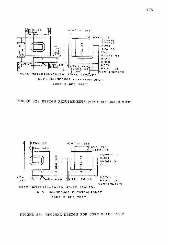
125
-. |<!-BF = . 1 E
]tz-l:''f~V:
|ln"ou1J >
CORE MATER IOL=EO,-EO NI-FE (SOflD)
D.C. HORSESHOE ELECTROMA GNE T
CORE SHOFE TEST
G X= it 4- EGN=#3 E
RW= 1
I X= O 3
V= 3
BX= IE 41
HX= E
HN=0
NOTE
D IMS I N
CENTIMETERS
FIGURE 32: DESIGN REQUIREMENTS FOR CORE SHAPE TEST
-
F .)= . O T
<r-W=. 03 4-
J X
J%. S
C D =
. 3 3?
II
3o
Jv
-C1 =
. LW= T 3 T
K-BF=. 1 E
"T"
WG = # 1 1 4-
R W= 1
N=30 1 .3
|*o. 1 E E - O 3NOTE .
DIMS. IN
CENTIMETERS
CORE MATER IAL= EOX EO NI-FE (SOLID)
D C HORSESHOE ELECTROMAGNET
CORE SHAPE TEST
FIGURE 33: OPTIMAL DESIGN FOR CORE SHAPE TEST

126
IX
o
u.
I
Ul
a
MO L TO G E
UOLTAGE AND AIRGAP SENSITIUITV FOR CORE SHAPE TEST
GAP
1 . 5E-03
1 . 5E-03
1 . 5E-03
1 . 5E-03
1 . 5E-03
1 . 5E-83
1 . 5E-03
1 . 5E-03
1 . 5E-83
5E-835E03
5E-03
5E-03
UOLTAGE
.5
1
1.5
2
2.5
3.5
4
4.5
5
5.5
6
6.5
IDEAL FORCE<02 3)
1.54314613
5.51705504
14.490173
25.3141497
38.2887021
49.6827594
54. 1494388
59.7893711
62. >41 -83
6c> . 241'
jilf> c>
63. 8669531
64.4971118
65. 1357818
FIGURE 34: GAP AND VOLTAGE SENSITIVITY FOR CORE SHAPE TEST
WITH LISTING FOR FIRST GAP ONLY

127
SAMPLE RUN FOR A SINGLE BOBBIN, UNCONSTRAINED CORE
SUBJECT TO THE STANDARD LIMITS OF THIS PROJECT
COIL NAME: CORE SHAPE TEST
COIL TYPE: SINGLE BOBBIN, RECTANGULAR CORE
OPERATING VOLTAGE: 3
COIL RESISTANCE: 85. 7247655
CORE MATERIAL: 50/50 NI-FE (SOLID)
THEORETICAL, NO LOSS HOLDING FORCE(OZ ): 49. 6827594
EXPECTED HOLDING FORCE (OZ ): 31. 796966
****PHYSICAL DIMENSIONS & CONSTANTS****
OVERALL LENGTH: 2. 00841072
OVERALL DEPTH:. 635277121
OVERALL WIDTH: .995048396
FLANGE WIDTH:. 0703393029
WINDING LENGTH:. 767040924
BOBBIN WALL THICKNESS :. 064
BOBBIN FLANGE THICKNESS :. 15
ARMATURE/BOBBIN CLEARANCE : . 2 8 5
WINDING CLEARANCE : . 0 7
AIRGAP: 1.5E- 03
STEEL PATH LENGTH : 4 . 42550004
CORE WIDTH:. 328184895
CORE DEPTH:. 366598515
CORNER RADIUS: .0141314864
CORE PERIMETER:1. 36530568
CORE AREA:. 120140672
AIRGAP AREA (FRINGING) :. 121166419
WINDING SURFACE AREA: 1 . 69468826
************* *WINDING DATA**************
WIRE GAGE NUMBER: #41. 4200803
TURNS SPECIFIED: 901. 266209
TURNS POSSIBLE:901. 266208
RANDOM WIND:1
WINDING WIDTH: .0703393029
BARE WIRE DIA:6.77459784E-03
OHMS/CM OF WIRE:. 0478352381
EFFECTIVE INSUL.WG : 40. 2742177
INSULATED WIRE DIA: 7 .73716314E-03
THEORETICAL TURNS/SQ CM=167 04 . 6158
CURRENT AT 3 VOLTS :. 0349957213
AVERAGE TURN LENGTH: 1. 988406 97
INDUCTANCE, HENRIES:. 3 73 005434
S.S.TEMP RISE, DEG C:61. 4507456
FIGURE 35: ANALYSIS LISTING FOR CORE SHAPE TEST
(CONTINUED ON NEXT PAGE)

128
(SAMPLE LISTING CONTINUED)
THERMAL TIME CONST: 136 . 577254
RESISTANCE @S. S. TEMP : 99. 7143539
CURRENT THAT TEMP :. 0300859393
IDEAL FORCE @THAT TEMP @3VOLTS=39. 7441485************ *MAGNETIC DATA* ************
TOTAL AMP-TURNS ( ACTUAL ) : 3 1 . 540461
TOTAL AMP-TURNS (AIR+IRON) : 31. 3672126AMP-TURNS IN IRON: 2 . 83035554
AMP-TURNS IN AIR: 28 . 536857
OERSTEDS IN IRON: . 803689898
OERSTEDS IN AIR: 11953 . 4907
KILOGAUSSES IN IRON: 12 . 0555482
KILOGAUSSES IN AIR: 11. 9534907
IRON SAT KILOGAUSS:15.41
***********DESIGN CONSTRAINTS***********
MAX OVERALL LENGTH: 2. 01
MIN OVERALL LENGTH :0
MAX OVERALL DEPTH:. 63 5
MIN OVERALL DEPTH :0
MAX OVERALL WIDTH: 1.01
MIN OVERALL WIDTH :0
MAX CORE WIDTH:. 5
MIN CORE WIDTH :0
MAX CORE DEPTH : . 5
MIN CORE DEPTH :0
MAX CORE CORNER RAD:. 2 5
MIN CORE CORNER RAD:0
MAX CURRENT @ 3 VOLTS:. 03 5
MAX WIRE GAGE NUMBER: 45
MIN WIRE GAGE NUMBER: 35
MAX KILOGAUSS IN CORE: 15. 41
DESIGN HINTS:
IF ANY FINAL DIMENSIONS ARE AT OR NEAR
THEIR LIMITS, THEN CHANGING THOSE LIMITS
MAY CHANGE THE FINAL SOLUTION.
TEMPERATURE RISE CAN BE REDUCED BY
INCREASING THE SURFACE AREA (OR LX)
FIGURE 35: ANALYSIS LISTING FOR CORE SHAPE TEST (cont)
129
11.3 Observations and Conclusions
The computer program has found a definite maximum for
each of the bobbin configurations. To check if they are
unique, the test for equivalent designs described at the end
of section 10.3 has been tried on the single round, and
single rectangular bobbin configurations. After making three
design runs with each type, no difference was found between
runs. While this is not a rigorous test, it is strong
evidence that the designs are unique, for the constraints
imposed, since the different start points generated for each
run should have ended in slightly different solutions, in the
event of equivalent configurations.
Most of the points about the physical dimensions for the
Production Design have already been discussed in Chapter II,
and will not be repeated here. One point which will be made
is that the bobbin is underfilled more than the amount which
would be expected for winding allowance. From figure 15, it
can be seen that the winding width is 0.042cm less than the
flange width. It is this condition which accounts for the
biggest difference between this design and the optimized
design using the same bobbin configuration.
When first viewing the sensitivity graphs, a common
observation is that they do not look right. Because the
three gaps are equally spaced, it is felt that theapparent
space between adjacent curves should be the same. The
difference in their appearance turns out to be an optical
130
illusion since, in fact, they are the same distance apart.
The calculations which follow will help to tie together the
discussion in Chapter II, the sensitivity graphs, and the
experiments which are covered in Chapter XII. m the
discussion which follows, it will be assumed that the airgap
difference between any two curves in a sensitivity plot is
unknown. This will result in a full excercising of the
thought process being developed. Figure 14, will be used as
an example.
Equation (25), can be rearranged so that for any known
force, the corresponding effective flux density can be
calculated.
BA =,/FT / Kl /AG'
(60)
For the small airgaps involved, it can be seen from
equation (19), that the area of the gap, AG, is essentially
constant for the small gaps discussed in this paper. This
simplification is most valid if AG, for the center curve, is
used.
With the simplification that AG is constant, equation
(60), is not directly dependent on the length of the airgap.
Thus, for any specific force level, the flux density in the
air will have a unique value, regardless of which airgap
curve is chosen. Since the core area is constant and the
area of the airgap is essentially constant, then equation
(23), states that this force level will also correspond to a
specific flux density in the iron, BI.
131
From the initial magnetization curve, it is known that
the relationship between B and H, for any one material, is a
single valued one. Because the flux density in the iron, BI,
is a unique value for any given force, it follows that HI, is
also unique. Finally, from equation (15), it can be seen
that the amp turns in the iron, NI, is similarly known since
the iron path length, PL, is a constant.
NI = HI * PL / PI / 0.4 (61)
Equation (20), dictates that the total amp turns in the
system is equal to the sum of the amp turns in the iron and
those in the air. It has been shown that for any given force
level, the amp turns in the iron is a constant. Therefore,
at that force level, for any number of total amp turns in,
the amp turns in the air can be calculated. Stated slightly
differently, since NI, is a constant then for any change in
NT, along a constant force line there will be an equal change
in NA.
d(NT) = d(NA) (62)
For a given coil, the number of turns is a constant.
Similarly, the total coil resistance is also a constant. By
equation (10), it follows that for any voltage, the current
is known. Multiplying the current by the number of turns
gives the total amp turns for the coil.
NT = NC * V / CR (63)
A combination of equations (62) and (63), results in
equation (64).
132
d(NA) = d(V) * (NC / CR) (64)
A combination of equations (14) and (15), results in
equation (65), which relates BA, NA and G. The constant of 2
is needed to account for the two airgaps. To keep the units
of BA consistently in kilogausses for this section, rather
than mixing with the gauss specified by equation (14), BA is
multiplied by a factor of 1000.
1000 * BA = HA = 0.4 * PI * NA / G / 2 (65)
By rearranging (65), the airgap, G, can be calculated
for any known NA and BA.
G = 0.4 * PI * NA / BA / 2000 (66)
From the sensitivity graph, NA is not directly known if
the situation existed where the gap was not known. However,
if two different gaps exist at the same value of BA, and thus
of force, then the difference between them is expressed by
equation (67).
d(G) = d(NA) * 0.4 * PI / BA / 2000 (67)
This relationship gives a very important piece of
information toward explaining the different slopes of the
three gap curves in any one sensitivity plot. For a fixed
airgap difference, the extra NA required to move from one
airgap curve to the next along a constant force line,
increases for increasing force directly proportional to the
corresponding increase in BA.
The logic in this argument has moved at a quick pace.
Hopefully the reader has followed it, as the arguments
133
presented will be used repeatedly in later sections. Many
different avenues of equation manipulations were tried before
the one just described was arrived at for explaining the
shapes of the different airgap curves. Except for two
implicit assumptions, the equations should result in a
precise prediction of differences in airgap for any one force
level. The first of these is the simplification that the
area of the airgap is essentially unaffected by changes in
the airgap. While this is very dependent on how large the
airgap is relative to the area of the core, for the
dimensions existing in any of the examples being considered
here, it is a reasonable simplification. Using the
Production Design, as an example, by equation (19), the gap
areas corresponding to airgaps of 0.0015, 0.003 and 0.0045
centimeters are 0.0894, 0.0903 and 0.0912 sq-cm respectively.
This is only a 1% change in area for gap steps which are
large relative to the airgaps.
The second assumption is that as the airgaps increase,
the flux leakages do not also increase significantly.
Section 2.10, alluded to a complex set of leakage paths at
the poles. One of the many factors determining these paths
is the airgap (Ref 11). Since no calculations have been made
for these leakages, the validity of this second assumption
will go unchecked in this paper.
The reasons for this complicated derivation will become
clearer in Chapter XII. It has been presented, at this time,
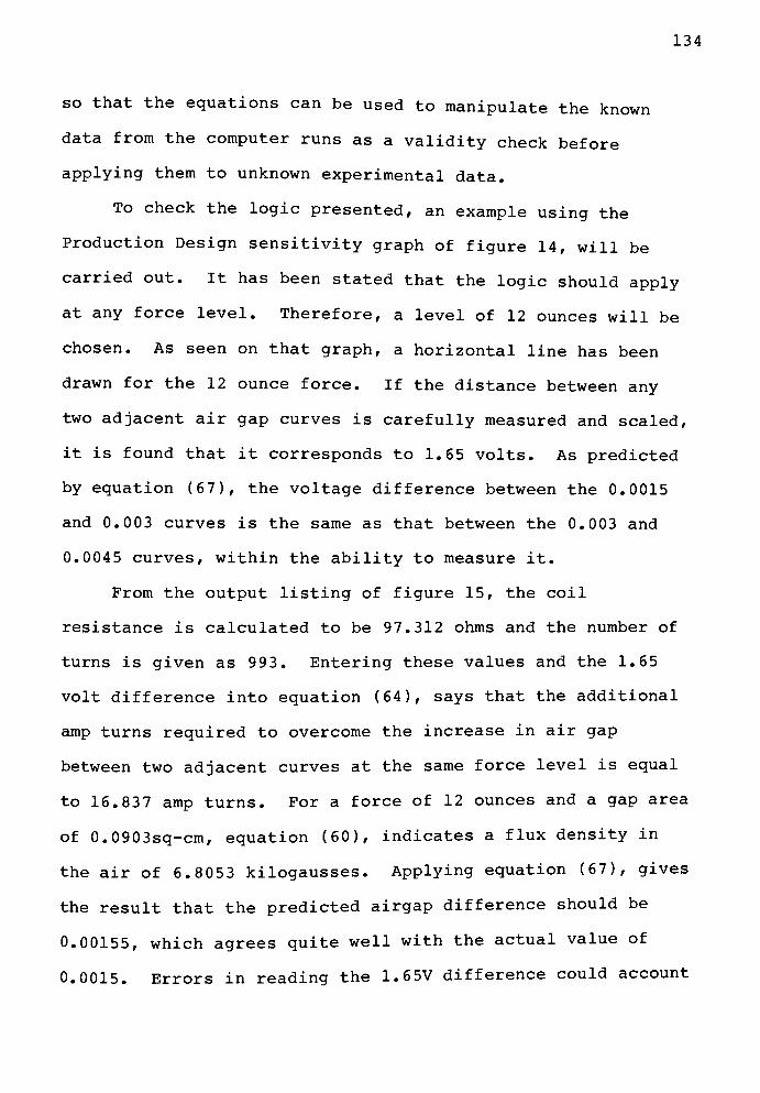
134
so that the equations can be used to manipulate the known
data from the computer runs as a validity check before
applying them to unknown experimental data.
To check the logic presented, an example using the
Production Design sensitivity graph of figure 14, will be
carried out. It has been stated that the logic should apply
at any force level. Therefore, a level of 12 ounces will be
chosen. As seen on that graph, a horizontal line has been
drawn for the 12 ounce force. If the distance between any
two adjacent air gap curves is carefully measured and scaled,
it is found that it corresponds to 1.65 volts. As predicted
by equation (67), the voltage difference between the 0.0015
and 0.003 curves is the same as that between the 0.003 and
0.0045 curves, within the ability to measure it.
From the output listing of figure 15, the coil
resistance is calculated to be 97.312 ohms and the number of
turns is given as 993. Entering these values and the 1.65
volt difference into equation (64), says that the additional
amp turns required to overcome the increase in air gap
between two adjacent curves at the same force level is equal
to 16.83 7 amp turns. For a force of 12 ounces and a gap area
of 0.0903sq-cm, equation (60), indicates a flux density in
the air of 6.8053 kilogausses. Applying equation (67), gives
the result that the predicted airgap difference should be
0.00155, which agrees quite well with the actual value of
0.0015. Errors in reading the 1.65V difference could account
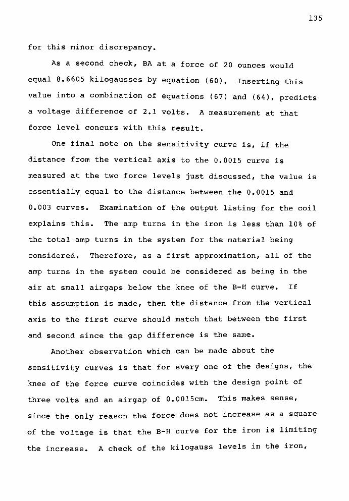
135
for this minor discrepancy.
As a second check, BA at a force of 20 ounces would
equal 8.6605 kilogausses by equation (60). Inserting this
value into a combination of equations (67) and (64), predicts
a voltage difference of 2.1 volts. A measurement at that
force level concurs with this result.
One final note on the sensitivity curve is, if the
distance from the vertical axis to the 0.0015 curve is
measured at the two force levels just discussed, the value is
essentially equal to the distance between the 0.0015 and
0.003 curves. Examination of the output listing for the coil
explains this. The amp turns in the iron is less than 10% of
the total amp turns in the system for the material being
considered. Therefore, as a first approximation, all of the
amp turns in the system could be considered as being in the
air at small airgaps below the knee of the B-H curve. If
this assumption is made, then the distance from the vertical
axis to the first curve should match that between the first
and second since the gap difference is the same.
Another observation which can be made about the
sensitivity curves is that for every one of the designs, the
knee of the force curve coincides with the design point of
three volts and an airgap of 0.0015cm. This makes sense,
since the only reason the force does not increase as a square
of the voltage is that the B-H curve for the iron is limiting
the increase. A check of the kilogauss levels in the iron,
136
for all designs, shows that they are all within 0.16 of 11.9
kilogausses. Referring to figure 2, it can be seen that this
corresponds to a point where the knee of the B-H curve has
just been passed. The designs have, therefore, optimized the
trade-off between increases in core area and flux density.
Increases in core area will increase the mean path length of
the wire. According to equation (12), this will result in a
decrease in total amp turns and, thus, a decrease in the flux
density. Since the force increases as the square of the flux
density and proportional to the area, this design exists
where the balance of the competing variables lie.
One of the objectives of the runs selected is to find
the best configuration of bobbin for the specified
constraints. This turns out to be the square core with a
double bobbin, which has a no-loss holding force of 51.2oz.
This is closely followed by the single bobbin square design
with 4 9.6oz. These are both approximately 50% higher than
the production design with only 3 5.6oz. The single round
design was only slightly better than the production one with
38.32oz, while the double round design finished a dead last
with only 27.2oz of no-loss holding force.
The core shape test is identical in every respect to the
single square bobbin design for all practical purposes. This
makes sense, since a rectangular bobbin utilizes the
available space more fully than a round one. The slight
differences between the core shape test and a purely
137
rectangular design would be lost in any manufacturing
process. No further mention will be made of this run except
to point out that during the search process, the R(25) and
R(26) inequality equations seem to have worked, since the
design did not wander off into imaginary space. When an
inequality does not work properly, this often happens. The
objective of this run is, therefore, met.
The major reason for the poorer performance of the round
designs can be found by comparing the overall depth. For
every one of the designs, the maximum length and width were
filled. For all the rectangular designs, the maximum depth
was also matched. In the case of the round designs, however,
the maximum width limited the size of the overall coil and
prevented the depth from reaching the allowed maximum. The
double round bobbin overall depth is only 3/4 of the amount
permitted by the design limits.
Steady state temperature rise is the only other factor
which showed a significant difference from among the four
basic types considered. Due to the decrease in surface area,
for the same power input, the single round bobbin exceeded
the 70 degree temperature difference allowed, while the other
three stayed below the limit. The double square design is
the best by a significant margin, being approximately half of
the value reached by the single square type. Even if the two
facing surfaces of the double design are considered to be
insulated, the double bobbin configuration has enough
138
additional surface area to stay cooler than the single one.
One final point of interest can be made by comparing the
predicted design from the first optimization method with the
same configuration bobbin in the second. In figure 6, the
locus of best designs was assumed to be somewhat symmetrical.
The result is a prediction that the core area should be
slightly less than 0.1225sq-cm, with a wire number near 41.5,
and a holding force of 50oz. The force of the final design
is 49.6oz, the wire gage 41.49 and the area 0.124sq-cm. This
is as close to a perfect match as can be expected. The minor
difference in area indicates that the locus of maximum
designs should have been skewed slightly to the right,
thereby aligning itself even closer with the
(CA)* (NT)* (NT) /PL line. The design methods can, therefore,
be treated as equally good for the constraints considered,
and it can be considered the designer's choice for which
method to use. Each has advantages and disadvantages which
must be weighed when choosing a method to use.
For the design constraints of the example problems, a
designer must choose the bobbin style that best suits his
needs. If the only factors to be considered are holding
force and temperature rise, then the double rectangular
bobbin is a clear winner. This must be weighed against the
complication to the manufacturingprocess caused by the
interconnection between the two bobbins. A further
manufacturing concern is that the wire is more prone to
139
breakage during the winding process with a rectangular core
than a round one. This is a result of the dynamic loads
imposed on the wire as the winding radius fluctuates on the
rectangular design. The radii on the bobbin walls have been
assumed to help alleviate this problem.
There are three items from the COIL DESIGN module output
which are not shown in any of the outputs in this paper.
They do not have any bearing on the solution, and the average
user would not be aware of their existence. The first item
is the number of basepoints required for the search process.
With the changes to the initial value of FP, between 55 and
63 basepoints, were required for the four basic types, while
the core shape test run required 96. Without the change to
FP, 272 points were needed for the rectangular core, single
bobbin design.
A second item of interest is the number of function
evaluations required. The four basic types took about 360
each, the core shape test, 548, and the unaltered single
square run, 152 9.
The last item of interest for those familiar with the
P519RE program is the number of resets required. This is an
indication of how many times the program ended up in a
corner. If the number of resets is too high, the answer
obtained becomes questionable. For the unaltered program,
this number was 14, which is more than is usually desired.
The other runs had a range of from two to six, which is not
140
unreasonable for a problem that has not gone through the
decomposition process.
In summary, the program met or exceeded all of its
goals, and produced useful results. All program modules
worked properly and the resulting package is easy to use and
highly user friendly. The point, which cannot be stressed
enough, is that the design calculated is the highest force
coil possible, subject to the given constraints. When an
actual sample is built, the somewhat arbitrary loss factor
may not be exactly correct, and as a result, the force
measured may vary slightly from the predicted number. With
the exception of manufacturing improvements affecting the
airgap, however, nothing will improve the potential holding
force within the constraints supplied. If more force is
required, then the requirements must be changed. Changing
the number of turns, wire size, or core area will only
decrease the performance of the coil for unchanged
requirements .
CHAPTER XII
HOLDING FORCE EXPERIMENTS
12.1 Purpose of the Experiments
There are four reasons for running these experiments,
which can be summarized as follows:
1) Compare the computer run results with actual
assemblies
2) Determine the effective airgap to use in the
computer runs, based on force measurements
3) Determine if the 64% force loss constant used in the
ANALYSIS program module is reasonable. It must be remembered
that this factor affects only the absolute level of force
calculated, but does not affect the optimum design. If the
loss factor is off, only the scale of the force plot needs to
be changed
4) Find the effect of core density on the holding force
and B-H curve characteristics.
The fourth point needs some explanation. For the
production of high volume, low cost holding coils, the use
of solid stock is discouraged. The reason for this is that
in addition to the forming or punching operation required to
produce the initial core blank, a grinding operation must be
performed to achieve good pole faces. This secondary
operation can increase the costs appreciably. Thealter-
141
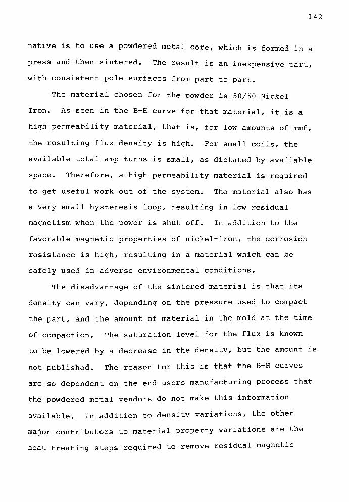
142
native is to use a powdered metal core, which is formed in a
press and then sintered. The result is an inexpensive part,
with consistent pole surfaces from part to part.
The material chosen for the powder is 50/50 Nickel
Iron. As seen in the B-H curve for that material, it is a
high permeability material, that is, for low amounts of mmf,
the resulting flux density is high. For small coils, the
available total amp turns is small, as dictated by available
space. Therefore, a high permeability material is required
to get useful work out of the system. The material also has
a very small hysteresis loop, resulting in low residual
magnetism when the power is shut off. In addition to the
favorable magnetic properties of nickel-iron, the corrosion
resistance is high, resulting in a material which can be
safely used in adverse environmental conditions.
The disadvantage of the sintered material is that its
density can vary, depending on the pressure used to compact
the part, and the amount of material in the mold at the time
of compaction. The saturation level for the flux is known
to be lowered by a decrease in the density, but the amount is
not published. The reason for this is that the B-H curves
are so dependent on the end users manufacturing process that
the powdered metal vendors do not make this information
available. In addition to density variations, the other
major contributors to material propertyvariations are the
heat treating steps required to remove residual magnetic
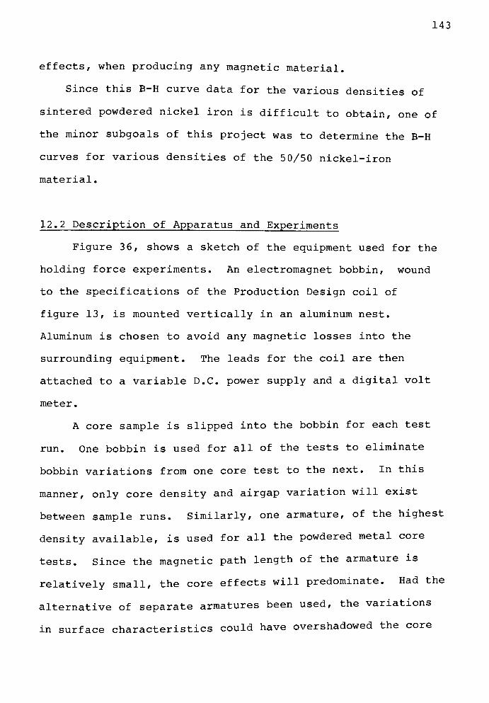
143
effects, when producing any magnetic material.
Since this B-H curve data for the various densities of
sintered powdered nickel iron is difficult to obtain, one of
the minor subgoals of this project was to determine the B-H
curves for various densities of the 50/50 nickel-iron
material.
12.2 Description of Apparatus and Experiments
Figure 36, shows a sketch of the equipment used for the
holding force experiments. An electromagnet bobbin, wound
to the specifications of the Production Design coil of
figure 13, is mounted vertically in an aluminum nest.
Aluminum is chosen to avoid any magnetic losses into the
surrounding equipment. The leads for the coil are then
attached to a variable D.C. power supply and a digital volt
meter.
A core sample is slipped into the bobbin for each test
run. One bobbin is used for all of the tests to eliminate
bobbin variations from one core test to the next. In this
manner, only core density and airgap variation will exist
between sample runs. Similarly, one armature, of the highest
density available, is used for all the powdered metal core
tests. Since the magnetic path length of the armature is
relatively small, the core effects will predominate. Had the
alternative of separate armatures been used, the variations
in surface characteristics could have overshadowed the core

144
VARIABLE D.C. POWER
SUPPLY WITH DIGITAL
VOLTMETER
LINKS FOR
TORQUE
ISOLATION
PRODUCTION DESIGN BOBBIN
WITH TEST CORE INSERTED
CUP FOR
WEIGHTS
CBBSsD
SKETCH OF APPARATUS
note: bobbin held vertical
in an aluminum nestENLARGEMENT OF ARMATURE
CROSS-SECTION AND HOLDER
SHOWING CENTERING FEATURE
figure-36: Holding Force Experiments Equipment
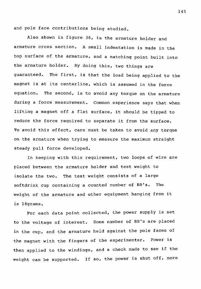
145
and pole face contributions being studied.
Also shown in figure 36, is the armature holder and
armature cross section. A small indentation is made in the
top surface of the armature, and a matching point built into
the armature holder. By doing this, two things are
guaranteed. The first, is that the load being applied to the
magnet is at its centerline, which is assumed in the force
equation. The second, is to avoid any torque on the armature
during a force measurement. Common experience says that when
lifting a magnet off a flat surface, it should be tipped to
reduce the force required to separate it from the surface.
To avoid this effect, care must be taken to avoid any torque
on the armature when trying to measure the maximum straight
steady pull force developed.
In keeping with this requirement, two loops of wire are
placed between the armature holder and test weight to
isolate the two. The test weight consists of a large
softdrink cup containing a counted number of BB's. The
weight of the armature and other equipment hanging from it
is 18grams.
For each data point collected, the power supply is set
to the voltage of interest. Some number of BB's are placed
in the cup, and the armature held against the pole faces of
the magnet with the fingers of the experimenter. Power is
then applied to the windings, and a check made to see if the
weight can be supported. If so, the power is shut off, more

146
weight added to the cup, and the process repeated until the
magnet can no longer hold the trial weight. The last load
which can be reliably held, is recorded as the holding force
for the device. One important point is that the power is
applied to the coil for only a short period of time in an
attempt to circumvent heating problems.
When the airgap experiment is run, shims are placed
along the full face of the armature, and the holding force
trials are run as described above. Five different shim stock
thicknesses have been tried. The thinnest three consist of
one, two and three thicknesses of clear wrapper from a
cigarette package, measuring approximately 0.0019cm each.
The two thickest spacers are pieces of brass of the thickness
specified.
12.3 Experimental Results and Calculations
The first experiment uses the shims described above to
determine the relative size of the airgap between the
unaltered poles and armature. Figure 37 shows the results in
graphical form. For the graph shown, one core and armature
of the highest density of sintered 50/50 Ni-Fe available is
used. This corresponds to the 16-ton sample, which will be
described later. Due to the uncertainty zone about the
actual holding force, the midpoint between the weight, which
could be held consistently, and one which could not be held
at all, has been recorded to the nearest 10 BB's. One BB has
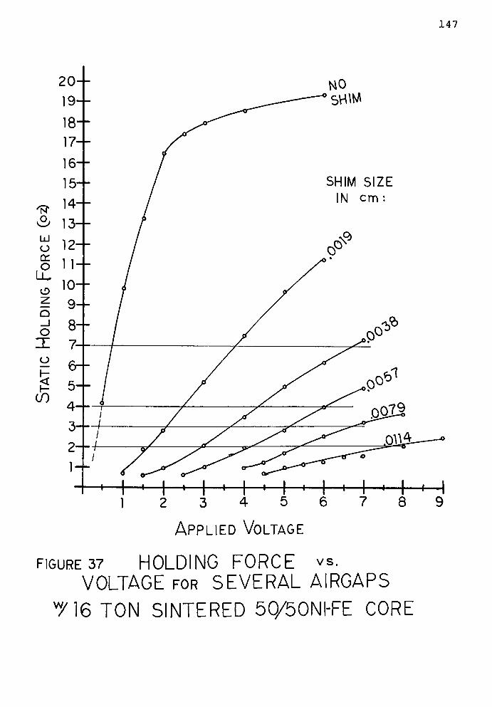
147
NO
SHM
ft
UJ
o
OC
o
z
Q
_J
o
IE
o
I
i ' i i i i
Applied Voltage
figure 37 HOLDING FORCE vs.
VOLTAGE for SEVERAL AIRGAPS
T16 TON SINTERED 50/50NI-FE CORE
148
an average weight of 0.34 5 grams, and the range of
uncertainty is on the order 10 BB's.
It can be seen that the trend of force versus airgap is
the same as that previously shown in the sensitivity graphs
from the computer runs. If, however, equation (67), is
applied to the difference between neighboring airgap curves
the calculated voltage difference is approximately half of
that actually measured. The initial concern was that the
equations, which have been developed, ignored the fact that
there are two airgaps in the system. A careful check has not
detected such an error, though one might exist.
Unfortunately, the equations used in the computer programs,
and those used to perform the sensitivity analysis in section
11.3, are the same. Therefore, it makes sense that they be
self-consistent. At this point in time, one possible
explanation for the discrepancy appears to be that the losses
are larger than expected. A factor of two seems too large,
however.
A second, more plausible explanation, lies in the size of
the gaps being considered. Since the shims are of the same
relative size as an airgap between two"flat"
surfaces, and
since the airgaps in the test are created by multiple layers
of material, it is very probable that each of the shims, plus
the surfaces between them, are effectively making a double
contribution .
Recognizing that a discrepancy exists, the concepts
149
which lead to equation (67) should apply even if the equation
does not produce the exact answer. With this, if it is
assumed that all the amp-turns available are in the air for
the no shim curve, then the ratio of the distance between the
vertical axis and the no shim curve, and the distance between
the no shim curve and 0.0019cm shim curve, should be equal to
the ratio of the airgaps. The actual airgap will be slightly
smaller than this, although any errors will be small for a
high permeability material. When measured at the 2,3,4 and 7
ounce force lines, there is an average ratio of 4.07. The
range of values is from 3.94 to 4.28 with no order to them.
Using this ratio, the effective airgap should be approximated
by a value equal to one fourth the 0.0 019cm gap difference
between the first two curves. Thus, a gap of 0.00047cm might
be assumed for each airgap for a 16-ton part. This is one
third of the value used in the computer runs. If, however,
the discrepancy between the predicted and apparent airgaps is
taken into account, the gap could be double this value, or
0.00094cm.
In actual practice, it is better to design for the larger
airgap expected. Then, holding forces will only improve with
improved manufacturing processes. The computer runs are
still valid, and the airgap chosen is less than 0.001cm
larger than the value inferred by the experimental results.
Any surface imperfection will more than mask this difference.
In addition, the sample used for the test happens to be the
150
best of four tried, so that any other one would have given a
different result. The direction of that change is to larger
airgaps. A final point is that the solid core force
experiment will demonstrate an apparent airgap of 0.0011cm.
Therefore, all values indicate that the first guess for an
airgap between two flat surfaces is a good one, and should
continue to be used.
12.4 Core Density Experimental Results
A graph of the data for the second experiment of force
versus voltage for different core densities is shown in
figure 38. When the parts of different density were
manufactured for these samples, the same amount of 10 0 mesh
powder was inserted in the die before pressing. The result
was a series of parts of all the same weight, but of
different thickness. To allow the use of one bobbin, and to
eliminate cross sectional area variation, the parts were
ground to the same thickness as the thinnest part. They were
then hydrogen annealed to remove the internal stresses
induced by the machining operation. These stresses can
significantly affect the magnetic characteristics of a
magnetic material.
A plot of measured part density as a function of press
tonnage is shown in figure 39. Only one cubic shaped sample
of each material measuring 0.25cm on a side was used in
making these density measurements. For this reason, small
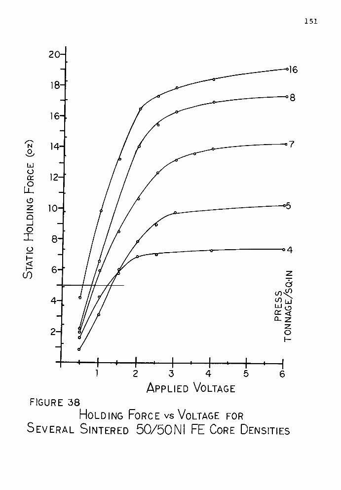
151
20-
18-
16-
3,
14-
o
OC12-'
o
Q
_J
o
X
10-.
8-
o
1-
6-'
CO
'I'l1 2 3 4 5 6
Applied Voltage
FIGURE 38
Holding Force vs Voltage for
Several Sintered 50/50NI FE Core Densities
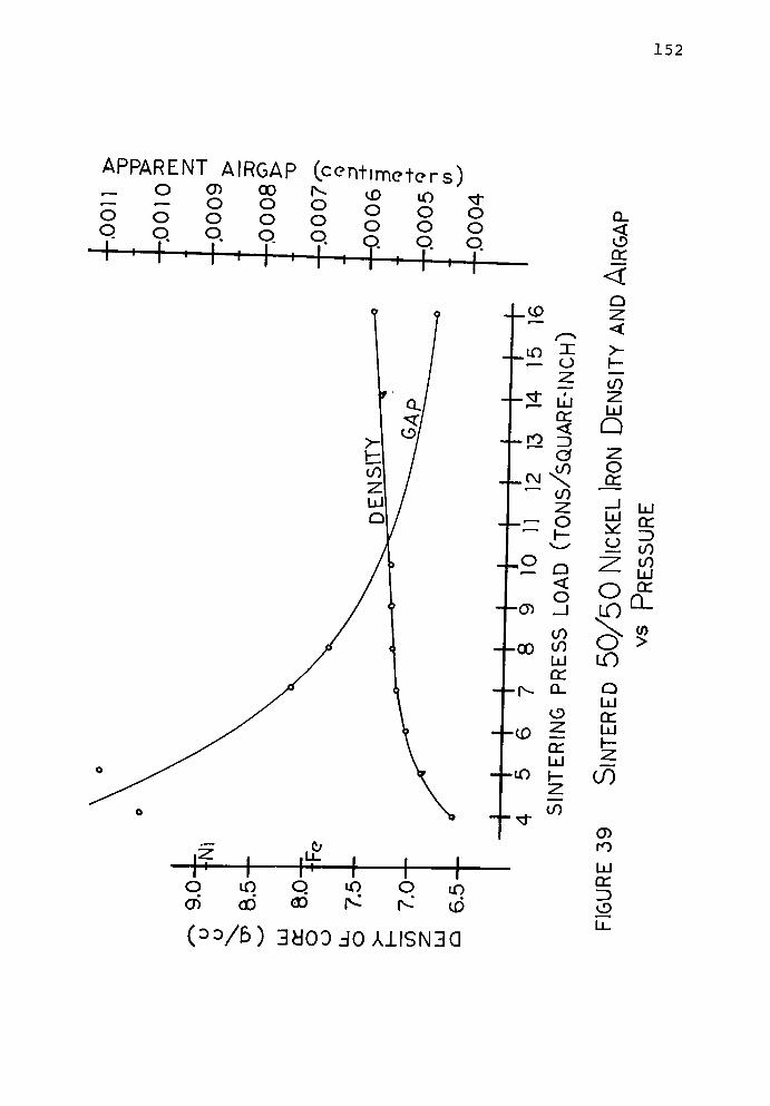
152
APPARENT AIRGAP (centimeters)
s2 S S go o o o o
Q? ? 9 ?
o
o
Q
f
+-> 5
ro
UJ
CC
<
a
CO
-- o
-_o
..O)
<o
CO
--00 CO
UJ
OC
a.--(V,
--CD
--if)
#-7+o lO
,to
4-*--+
c3
3Z
CC
LUf-
CO
Q to
H 1O iO
CD
(/B) 3UO0 J0A1ISN3Q
CL
3OC
<
h-
2 55
UJ
Q
occ
UJ
OC33
UJ
y c/>
m
Q
UJ
CCUJh-
CO
rO
UJ
OC
3O
u_
153
errors in weight or size, plus material defects, could
greatly affect the absolute values calculated. What is
important in figure 39, is the relative change in density
with pressure. It can be seen that definite improvements in
density result from increases in the pressure up to 8 tons
per square inch. Above this point, the returns are small,
and the likelihood of tool breakage large.
The force versus part density graph of figure 38, shows
this same trend. Large relative improvements in holding
force are experienced for increases in density up to the
density corresponding to 8-tons pressure. A doubling of the
8-ton pressure, however, yields only a 10% increase in
holding force.
In addition to the higher holding forces, a second piece
of information can be obtained from figure 38. Down at the
lower end of the curves, it can be seen that there is a
displacement horizontally, which tends to move to the right
as the density decreases. This can be the result of one of
two phenomena. The first would be that as the part density
decreases, more surface irregularities occur and, therefore,
the effective airgap increases. By measuring the voltage
difference between curves for one force level, it should be
possible to calculate those airgaps by the techniques
developed in this paper. These have been carried out,
assuming the 0.0019cm airgap difference between the first two
curves, and are shown in figure 39. If this is a cause and
154
effect, the trend is very definite for the points chosen.
The absolute airgaps might be in error by the factor of two
discussed previously, but the trend should be correct.
The second possible explanation for the displacement
could be found with the B-H curves for the material. When
making the airgap calculations, it is assumed that the flux
density and amp turns in the iron are the same for any give
force. If, however, there is a difference in the amount of
mmf required to reach a specific flux density for each of the
materials, then the airgap calculations are invalid. This
difference could be the result of either a shift of the B-H
curve to the right with density decreases, or a vertical
scaling of the B-H curve with density. Without the B-H
curves, it is difficult to predict which theory best explains
the effect. This is the intent of the experiment presented
in Chapter XIII.
12.5 Solid Core Experimental Results
Using a solid nickel iron core and armature, the holding
force measurements were repeated for this experiment. A
different armature was required, because the sintered
material armature could become the limiting factor on the
amount of flux which the iron path passes. This concern is
based on the results of the previous experiment. Since the
density of the 16-ton part is less than that of solid nickel
iron, and since it has been shown that density affects the
155
holding force and, thus, the flux density, the concern is
justified. A second solid core was, therefore, cut and used
as an armature.
Two additional remarks need to be made concerning the
core used for the test. The first is that the amount of
protrusion above the bobbin, CI, is only 0.038cm. A check
with the computer reveals that this has only a very small
affect on the expected holding force. A difference of only
0.25 ounces out of 50 is likely. The second note is that
during the manufacturing process, the core necked down
slightly at the bend during the bending operation. Section
2.10 indicated that this section of the core saturates first.
Therefore, this area is likely to be the limiting section of
metal path. As a result, expected flux densities might not
be reached, or at the very least, deviations of the holding
force near the knee of the B-H curve knee can be expected.
Figure 40, shows the plotted experimental results. The
force level reached at the maximum of 6 volts is more than
fifty percent higher than that attained by the best sintered
core. The earlier assumption, therefore, which determined
the need for a solid armature, is correct.
One of the goals of these experiments is to determine
how closely the computer trials predict the actual
performance of an assembly. To do this, an airgap must be
assumed, and the force loss multiplier checked. When the
solid core experimental results are compared to the results
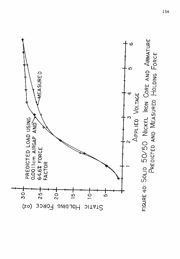
156
--
CD
(zo) aoacy oniqhoh onvis
) cc
31-
< UJ
2 oQC cc
<oQ_
Q
2 CD
< ^Q
LU_j
UJ
CD
O nr
2_J
_j <Q UJ UJUJ
??2ZI o
Q_
<2_
<
O_
!P S\ \-
O o
LO Q
UJ
2_l
O
CO
6sf
UJ
cc
3CD
157
from the core density experiment, the solid core plot is not
parallel to the other curves. It is slightly steeper, and
falls between the 5-and 8-ton lines. Taking the average
airgap for the samples, and assuming the theory that the
effective airgap is larger than the shim thickness due to the
extra surfaces of the shims, an airgap of 0.0011cm per pole
is assumed for the solid sample.
A computer run is then made using this gap and the
shorter core protrusion value. The predicted no loss holding
force is compared with the measured force at six volts, and
the ratio taken. Using this ratio as a force loss
multiplication factor, the computer prediction and
experimental data can be compared.
The result is shown in figure 40. The derived
multiplication factor is 0.645, which is nearly identical
with the 64% factor assumed during the initial computer runs.
Therefore, for the configuration presented, the assumed loss
factor can be used with confidence. Future trials with
different configurations will be required to determine if the
complex loss factors should be added to the program to
account for alternate designs.
From the graph, it can be seen that the experimental and
predicted values are identical until the knee of the force
curve is reached. This can be due to any combination of
three factors. l)The core necking, which has been presented
earlier, 2) loss factors which require more mmf to produce the
158
expected flux density than predicted or 3 ) experimental error.
Regardless of which combination of factors is chosen, the
conclusion is that the computer predictions agree even more
closely than might normally be expected. In addition, gap
lengths and loss factors are reasonable. More important, the
method, for determining the airgap from gap curves developed
for this project, does work. Gaps created at the interface
between shims is, therefore, the likely explanation for the
discrepancy described earlier. At this point, the B-H curves
for the sintered samples are not available and, therefore, a
similar set of calculations cannot be made for that
experimental data to further strengthen the validity of the
methods developed and presented herein.
12.6 Observations and Conclusions
Even if the airgap calculation method discrepancy is not
correctly explained by the extra gaps at the shim interfaces,
a number of checks can be made on the equations and
assumptions presented with the experimental data. One of
these is shown by the graph in figure 41. Here, equation
(60), has been used to calculate the flux density
corresponding to loads of 2,3,4 and 7 ounces. The gap area
has been assumed to be 0.089sq-cm. The data from the force
versus airgap experiment, (figure 37), is then plotted as the
voltage needed to overcome an increase in airgap versus the
calculated flux density. A family of lines results. Each

159
AIRGAP INCREASEOVER NO SHIM
MEASURED FORCE (02)2 3 4 7
H1 <c 6 4 5
Calculated Flux Density (kilogausses)figure 41
Voltage Increase vs Flux Density for
Fixed Airgaps
160
one corresponds to a different gap increase over the no shim
case.
The key to understanding this graph, is that it is the
increase in voltage to overcome the additional airgap that
is plotted on the vertical axis. Any material B-H
relationships have been accounted for in the no shim curve.
If equation (65), is applied at two different flux densities
for the same airgap and subtracted, equation (68). results.
d(BA) = d(NA) * (0.4 * PI / G / 2000) (68)
This should not be confused with equation (67), which applies
at a constant value of BA.
Since the only variables in equation (68), are BA and
NA, then the two should change in a linear manner. The fact
they do not in figure 41, supports the leakage equation (27).
It takes a larger number of amp turns in the air to produce
an equal change in the flux density, because the leakages
are increasing with flux density. Therefore, the constant
loss assumed by the adjustment to the total holding force in
the ANALYSIS program is not exactly correct, as described in
the discussion on leakage in chapter II. However, the solid
core experiment demonstrated that 64% is a good number for
the case being considered.
The data from figure 41 has been rearranged in figure 42
to show the increase in voltage over the no shim curve versus
the increase gap over the no shim curve as a function of the
force levels checked. Combiningequations (67) and (64), for
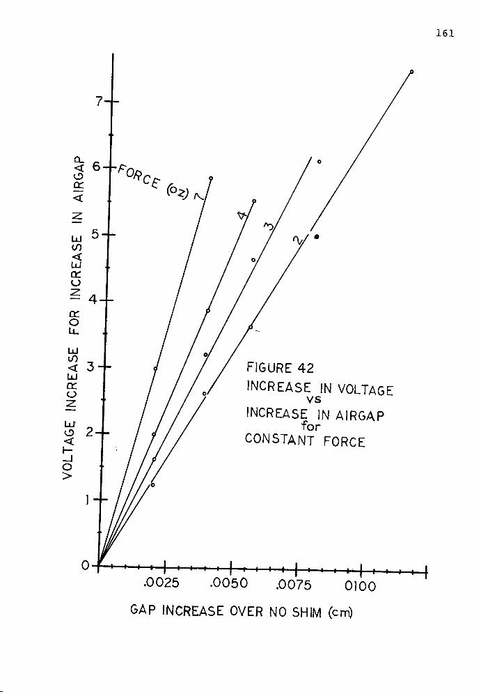
161
FIGURE 42
increase in voltagevs
increase in airgapfor
CONSTANT FORCE
+ - i t-
.0025 .0050.0075 0100
GAP INCREASE OVER NO SHIM (cm)
^
162
constant force lines results in equation (69).
d(G) = d(V) * (NC * 0.4 * PI / BA / CR / 2000) (69)
The change in the airgap driving voltage should be
proportional to the change in airgap for a constant BA. The
slope of the line should be given by the quantity in
parentheses in (69). Figure (42), bears this out, except for
the magnitude of the slope. It is off by the factor of 2,
mentioned earlier, which again implies that the measured and
effective gaps are different.
In conclusion, the general effect of changes in values
presented earlier in this paper are born out by the
experimental data. Without necessary B-H curves, further
checks cannot be made to strengthen the validity of the
project or suggest areas which need further investigation.
The next chapter will present the results of experiments
aimed at finding those B-H curves.
CHAPTER XIII
B-H CURVE DETERMINATION EXPERIMENT
13.1 Purpose of the Experiment
The goal of this experiment is to determine the B-H
characteristics of the various samples of sintered 50/50
nickel-iron used in the experiments presented in Chapter XII.
Due to problems encountered during the work and time
constraints, the full goal has not been realized. Partial
results will be presented for those wishing to complete the
task. The data, which would have been provided by this test,
is only needed to further substantiate the information
presented, and in no way is of primary importance to the
project.
13.2 Description of the Apparatus and Procedure
One core from each of the density samples was drawn for
the testing. One leg from each core was removed, and a
sample measuring 0.274cm square by 1.651cm of each was
ground. These were then passed through the normal hydrogen
annealing process to remove any residual magnetism and
internal stresses.
The samples were then placed in an AC Magnetometer for
measurement of the B-H curves. The theory of operation of
this piece of equipment is to have two coils around the
163
164
sample. An excitation coil is used to set up an alternating
magnetic field. A secondary coil is also located around the
sample along the same cylindrical axis as the primary coil.
The purpose of this secondary coil is to detect and measure
the strength of the magnetic field.
To make a measurement, a reading is first made with no
sample in the chamber. The knobs are then adjusted until no
signal is outputted from the secondary coil. This step is to
remove the B-H characteristics of air from the readings so
that only the material characteristics are measured. Samples
are then individually inserted into the chamber, and the
equipment varies the induced field between positive and
negative limits specified by the user. An integral computer
stores the data and displays the resulting B-H curve on a
monitor or paper print.
13.3 Presentation of Data
During the first trials, the B-H curves were measured
and plots produced. When they were compared to the curves
for solid nickel iron, the flux density levels at saturation
seemed reasonable. The location of the curve on the H axis
did not seem to agree, therefore, a second set of samples was
generated to make DC Magnetization measurements (Ref 12).
These samples had to be lighter than the first ones to be
compatible with that piece of equipment.
The set of samples were generated in a manner similar to
165
the first, with dimensions of 0.25cm cubed. When the data
was taken again with this second set of samples by the
alternate method, the same saturation levels were measured,
but the knee of the curve shifted by a factor of 10 on the H
axis. A return to the first method of measurement with the
second set of samples agreed with the readings from the
second method, which showed that a material sample dependency
existed.
The problem turned out to be an effect known as surface
demagnetization (Ref 13). This is a characteristic of the
surface of a material which counteracts the magnetic field.
It should be dependent on the geometry of the part only, and
not a function of the material being tested. If the
magnitude of the effect is known, then a demagnetization
correction factor can be applied to the B-H curve to
eliminate the condition, thereby, resulting in a curve which
is independent of the part geometry.
The sum of the correction factors for the three axes is
equal to unity. For a cube, the correction factor should be
1/3 for any direction perpendicular to one of its faces.
When this factor was tried on the samples, it did not work.
On some, the correction seemed to work, while on others, an
overcorrection was noted. It appeared that the material did
not behave homogeneously, so after considerable effort, the
investigation had to be dropped.
The curves shown in figure 4 3 are the uncorrected curves
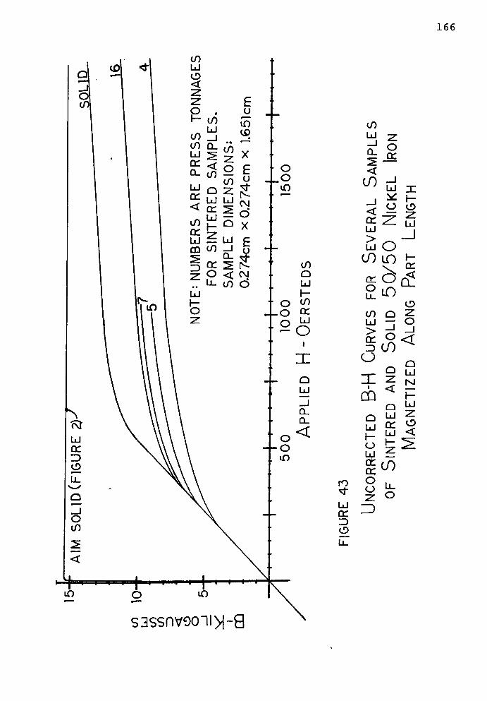
166
rO
U
CC
3cD
CO
<
^ ri X
_j
* h-
cc 2
o
UJUJ
> ^_l
ui O
CO LOi-
oc C5
cc
uoCD
C/) Q Z
UJ ; o
> -=i _J
CC
3C0<
oQ
X zz.UJ
Mu <
DQ1-
QUJ
Q U z
Zl uj
CD
<
o
OO
CO
U-
o
s3ssnvooii>|~a
167
for the first long samples, superimposed on one graph. The
curves represent the full B-H curve for the materials. For
those familiar with these curves, it can be seen that there
is no hysteresis loop to them.
Also shown are the measured flux density levels at the
extreme of the curves. The important thing to remember about
these uncorrected curves is that the vertical axis is right.
When the proper correction is applied, the shape of the curve
will change by a shifting of individual points toward the
vertical axis. The saturation level will not change.
13.4 Observations and Conclusions
It would be possible at this point to take the
information obtained by the above investigation, combine it
with the experimental results found earlier, stir in some
assumptions and arrive at a set of B-H curves for the various
densities of material. This way a relationship could be
sought which related the results with the density. The
relationship might result in a factor which could be
multiplied times the B-H curve for solid nickel-iron for use
in the computer program. Then a question could ask for the
material density and arrive at the information necessary for
designing or analyzing a coil.
After several hours of data manipulation, the exercise
was dropped. The effort was not compatible with the relative
importance of the information to the overall project.
CHAPTER XIV
CONCLUSIONS AND RECOMMENDATIONS FOR FURTHER STUDY
All the primary objectives of this project have been met
or exceeded. A maximum holding force configuration has been
demonstrated for each of the design constraint combinations
tested. In addition, the solutions all appear to be unique,
for each set of constraints, as described in sections 3.5 and
10.3. Several additional computer trials appear in Appendix
J, which show that no general conclusions can be drawn about
the best ratio of core volume to winding volume.
The first two trials analyze the TEST-SQ-S-D3 coil,
(Figures 16 through 19), with two different core materials.
The materials chosen are cold rolled steel and oriented 3%
silicon strip. This second material is usually available in
sheet stock, however, the trial was made to demonstrate a
material with a higher permeability than 50/50 Ni-Fe. As
expected, the holding forces are different with each core.
The final two trials demonstrate that the configuration
changes with core material. To make these runs, the design
constraints of the TEST-SQ-S-D3 coil have been retained, but
the material changed to cold rolled steel and 3% Si-strip.
The result is a different configurationfor each, with higher
holding forces than when those materials were inserted in the
TEST-SQ-S-D3 bobbin, indicating that optimization works.
168
169
Two complimentary methods of finding the optimum design
for a set of user defined constraints have been developed,
which arrive at the same solution. The second method
developed is extremely user friendly and requires no
knowledge of the program or magnetics to use. The intended
user is the mechanical designer who has an idea of the
approximate space available for an electromagnet, but has no
idea of the force potential for the volume present. This
program suits that user's need very well, and is a vehicle
for passing valuable experience. Future designers will not
have to go through the learning experience that has been
required to carry out this project.
The program is also a valuable analysis tool for an
existing design. It gives the designer many of the pieces of
information needed to determine the level of performance that
can be expected from a given design, and in the event of
minor changes, a feel for how the performance will be
affected by those changes.
A good data base has been started, with the experimental
results presented, for correlating the computer output to
actual electromagnet samples. The correlation for the single
configuration presented is very good. At this point in time,
it is felt that the program,equations and concepts developed
in the paper can be used confidently.
Several topics have gone uncovered or only lightly
presented, and deserve additional study. The first of these
170
is the completion of the B-H curve generation for the various
density samples of nickel iron. Some questions which would
have to be answered by this study include l)Why did one
correction factor not seem to work for all samples? 2)Why
does the factor for a cube not agree with published data?
3) Is there a relationship that can be fit to an equation
which relates the B-H curve for the solid nickel-iron
material to its less dense sintered counterparts? At first
thought, it would seem that the values of flux should be
directly proportional to the density. The reason for this
hypothesis is as follows: If it is assumed that the lowering
of density is the result of randomly spaced, microscopic
pockets of air, then the cross-sectional area of metal at any
point should be reduced by the presence of that air. On the
average, the metal should occupy a percentage of the cross
section proportional to the ratio of the part density to the
density of the solid metal. Examination of the flux
densities shown in figure 43, do not agree with this.
Conversely, the air might be considered to present a set
of small airgaps within the material. A model of the
magnetic properties of each grain would then have to be
devised, complete with surface demagnetization effects and
interactions with neighboring grains. This study could
become very involved and of a highly technical nature.
Another study suggested by this project is to include
the detailed loss coefficients in the ANALYSIS and/or DESIGN
171
modules to determine their effects on the final design. It
is not unthinkable that a different design could result if
these factors are taken into account. For example, the core
poles may tend to move apart, or the area of the core might
increase slightly, to reduce the flux density. This would
reduce the losses and increase the area. The resulting
design, would probably predict a lower force than that shown
by the methods developed for this project, but might come
closer to the actual force for all coil configurations. This
is not to say the methods developed here are not good,
because they provide a better tool than existed before. Any
method can be improved, and this one is no exception.
The idea suggested in section 2.10 could be pursued more
thoroughly. This involves increasing the cross-sectional
area of the yoke, and tapering it toward the poles in an
effort to combat the interpolar flux leakage. Ignoring the
manufacturing concerns, this study would determine if the
idea has any merit, or if some other factor counteracts the
flux loss gains to result in no design improvements.
Several improvements could be made on the program
package developed. For example, some simple code changes
could be made to allow the use of a second disk drive for
data storage, instead of using the program disk for that
purpose. This would permit write protection of the program
disk to reduce the possibility of erasure. Other
improvements relate to speeding up the package, such as
172
compiling the Basic program into machine code to reduce
computation time. Also, when using the ANALYSIS module, it
is necessary to return to the PAGE 2-A module and redraw the
coil picture before changes can be made. It would be
possible to either simply make changes in the ANALYSIS module
itself, rather than exiting, or to re-display the existing
picture with the correct POKE statements, since the values on
it have not changed. The first choice would eliminate the
time required to load each module while the second would
eliminate the long drawing time.
A more significant change would be to combine the two
optimization methods developed in this paper by using the
first method to find the start point for the search process
of the second method. The shotgun search works, but is
literally a hit-or-miss proposition. The first optimization
method would provide a more intelligent search for a good
starting point.
When working with a high production design, changes
during the life of the product are inevitable. Often, one of
the constraints imposed is that the fewest number of parts in
an assembly be affected. Currently the program is not well
suited for experimentation with existing parts. For example,
if it is desired to increase the holding force for a given
assembly, without changing any of the tooled parts, the only
variables left are the wire size and number of turns. It was
stated previously that a design determined by the
173
optimization processes developed in this paper will be the
maximum force permitted by the given constraints. One of the
givens must be modified, therefore, to have a difference in
the windings produce any force change.
Examination of the equation system reveals that either
the supply voltage or the permissible current draw must be
increased. In particular, equation 13, indicates that for a
fixed supply voltage, the total amp turns can only be
increased by a reduction in the average path or ohms per
centimeter of the wire. For a given bobbin, the average path
cannot be changed appreciably, therefore, the ohms per
centimeter is the only real variable. This implies that once
the bobbin and core geometries have been established, the
total number of amp turns is determined solely by the wire
gage used to wind it. The number of turns will only change
the total resistance. This discussion required a working
knowledge of the equation system. It would be an improvement
if the program could convey this information to the user.
In a similar manner, for a revision of the current
requirement, it might be desirable to determine which winding
width would be required for each available wire size to match
the required resistance. Referring to the equation system,
it is possible to combine equations 11, 1, 3 and 4 to arrive
at a quadratic equation for solving the winding width, WW.
A*WW**2+B*WW-CR/RW=0 (70)
Where A = PI * LW * W2 * OC (70a)
174
and B = (CP + 2 * Pi *w) * LW * W2 * OC (70b)
These manipulations are not difficult when the equation
system is known, but the average user is not well-versed in
it. It would be desirable to have these types of
calculations readily available and identified in the program.
A final topic of study would be to use the tools
developed to analyze the designs which would result from
different design constraints. Trends could be found, which
would aid a designer by setting up guidelines for what types
of bobbin shape is best. For example: Is a long slender coil
better or worse than a short fat one of the same volume?
Under what circumstances are double bobbins better than
single ones and vice versa? Is the round configuration ever
better than a rectangular one? The list could go on and on.
Based on the results of this study, samples could be built to
test the theory against reality.
In any study of this magnitude, as many questions have
been raised as have been answered. A good foundation has
been established, however, and merits building upon.

APPENDIX A
FIRST OPTIMIZATION METHOD
On the following page is the sample listing of a program
similar to the one used to generate the data for the plots in
chapter 3. Modifications have been made to include the wire
data curve fit equations developed in chapter 4.
175
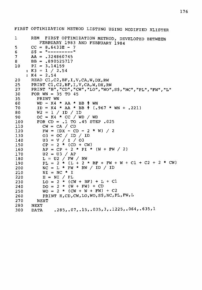
176
FIRST OPTIMIZATION METHOD LISTING USING MODIFIED XLISTER
1 REM FIRST OPTIMIZATION METHOD, DEVELOPED BETWEEN
FEBRUARY 1983 AND FEBRUARY 1984
5 CC = 8.6433E - 7
6 S$ =" "
7 AA =.324860745
8 BB =.890525717
10 PI = 3.14159
: K3 - 1 / 2.54
: K4 = 2.54
20 READ C1,C2,BF,I,V,CA,W,DX,RW
25 PRINT C1,C2,BF,I,V,CA,W,DX,RW
27 PRINT"H"
,
"CD"
,
"CW"
,
"LO"
,
"WO"
, S$ ,"NC"
,
"PL"
,
"FW"
,
"L"
30 FOR WN = 35 TO 45
35 PRINT WN
60 WD = K4 * AA * BB i WN
70 ID = K4 * AA * BB t (.967 * WN + .221)
80 W2 = 1 / ID / ID
90 OC = K4 * CC / WD / WD
100 FOR CD =.1 TO .45 STEP .025
110 CW = CA / CD
120 FW = (DX - CD - 2 *W) / 2
130 03 = OC / ID / ID
140 U3 = V / I / 03
150 CP = 2 * (CD + CW)
160 AP = CP + 2 * PI * (W + FW / 2)
170 U2 = U3 / AP
180 L = U2 / FW / RW
190 PL = 2 * (L + 2 * BF + FW + W + CI + C2 + 2 * CW)
200 NC = L * FW * RW / ID / ID
210 NI = NC * I
220 H = NI / PL
230 LO = 2 * (CW + BF) + L + CI
240 DO = 2 * (W + FW) + CD
250 WO = 2 * (CW + W + FW) + C2
260 PRINT H,CD,CW,LO,WO,S$,NC,PL,FW,L
270 NEXT
280 NEXT
300 DATA .285, .07, .15, .035, 3, .1225, .064,.635,1
APPENDIX B
PAGE 1 PROGRAM MODULE
B.l Program Listing 178
B.2 Program Length and Cross Reference 183
177
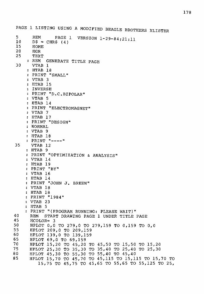
178
PAGE 1 LISTING USING A MODIFIED BEAGLE BROTHERS XLISTER
VERSION 1-29-84; 21: 115 REM PAGE 1
10 D$ = CHR$ (4)15 HOME
20 HGR
2 5 TEXT
: REM GENERATE TITLE PAGE30 VTAB 1
HTAB 18
PRINT "SMALL"
VTAB 3
HTAB 15
INVERSE
PRINT "D.C. BIPOLAR"
VTAB 5
HTAB 14
PRINT "ELECTROMAGNET"
VTAB 7
HTAB 17
PRINT "DESIGN"
NORMAL
VTAB 9
HTAB 18
PRINT" "
35 VTAB 12
HTAB 9
PRINT "OPTIMIZATION &ANALYSIS"
VTAB 14
HTAB 19
PRINT"BY"
VTAB 16
HTAB 14
PRINT "JOHN J.BREEN"
VTAB 18
HTAB 18
PRINT"1984"
VTAB 23
HTAB 5
PRINT "(PROGRAM RUNNING: PLEASEWAIT)"
40 REM START DRAWING PAGE 1 UNDER TITLE PAGE
45 HCOLOR= 3
50 HPLOT 0,0 TO 279,0 TO 279,159 TO 0,159 TO 0,0
55 HPLOT 209,0 TO 209,159
60 HPLOT 139,0 TO 139,159
65 HPLOT 69,0 TO 69,159
70 HPLOT 15,20 TO 45,20 TO 45,50 TO 15,50 TO 15,20
75 HPLOT 25,30 TO 35,30 TO 35,40 TO 25,40 TO 25,30
80 HPLOT 45,30 TO 55,30 TO 55,40 TO 45,40
85 HPLOT 15,70 TO 45,70 TO 45,115 TO 15,115 TO 15,70 TO
15,75 TO 45,75 TO 45,65 TO 55,65 TO 55,125 TO 25,

179
90
95
100
105
110
115
120
125
130
135
140
145
150
155
160
165
170
175
180
185
190
195
200
205
210
125 TO 25,115
HPLOT 15,110 TO 45,110
HPLOT 25,70 TO 25,65 TO 35,65 TO 35,70
HPLOT 104,20 TO 134,20 TO 134,50 TO 104,50 TO 104,20
TO 74,20 TO 74,50 TO 104,50
HPLOT 84,30 TO 94,30 TO 94,40 TO 84,40 TO 84,30
HPLOT 114,30 TO 124,30 TO 124,40 TO 114,40 TO 114,30
HPLOT 104,70 TO 134,70 TO 134,115 TO 74,115 TO 74,70
TO 104,70 TO 104,115
HPLOT 74,75 TO 134,75
HPLOT 74,110 TO 134,110
HPLOT 84,115 TO 84,125 TO 124,125 TO 124,115
HPLOT 84,70 TO 84,65 TO 94,65 TO 94,70
HPLOT 114,70 TO 114,65 TO 124,65 TO 124,70
HPLOT 154,70 TO 184,70 TO 184,115 TO 154,115 TO 154,70
TO 154,75 TO 184,75 TO 184,65 TO 194,65 TO 194,125
TO 164,125 TO 164,115
HPLOT 154,110 TO 184,110
HPLOT 164,70 TO 164,65 TO 174,65 TO 174,70
S = 1
ST = 154
H = 169
K = 35
R = 15
E = 184
GOSUB 545
ST = 184
H = 189
R = 5
E = 194
GOSUB 545
ST = 164
H = 169
E = 174
GOSUB 545
FOR I = 1 TO 5
READ X
HPLOT X,30 TO X,39
NEXT I
FOR I = 1 TO 7
READ X
HPLOT X,32 TO X,37
NEXT
DATA154,184,214,244,274,164,174,194,224,234 254 264
HPLOT 244,70 TO 274,70 TO 274,115 TO 214,115 TO 214,70
TO 244,70 TO 244,115
HPLOT 214,75 TO 274,75
HPLOT 214,110 TO 274,110
HPLOT 224,115 TO 224,125 TO 264,125 TO 264,115
HPLOT 224,70 TO 224,65 TO 234,65 TO 234,70
HPLOT 254,70 TO 254,65 TO 264,65 TO 264,70
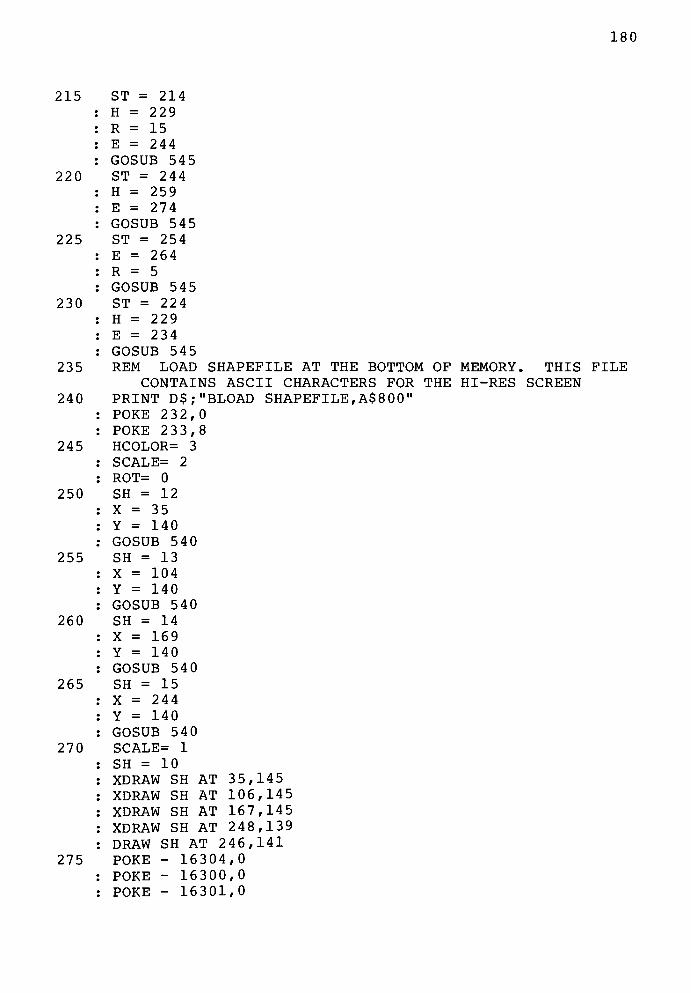
180
215
220
225
230
235
240
245
250
255
260
265
270
275
ST = 214
H = 229
R = 15
E = 244
GOSUB 545
ST = 244
H = 259
E = 274
GOSUB 545
ST = 254
E = 264
R = 5
GOSUB 54 5
ST = 224
H = 229
E = 234
GOSUB 545
REM LOAD SHAPEFILE AT THE BOTTOM OF
CONTAINS ASCII CHARACTERS FOR THE
PRINT D$;"BLOAD SHAPEFILE,A$800"
POKE 2 3 2,0
POKE 233,8
HCOLOR= 3
SCALE= 2
ROT= 0
SH = 12
X = 35
Y = 140
GOSUB 540
SH = 13
X = 104
Y = 140
GOSUB 540
SH = 14
X = 169
Y = 140
GOSUB 540
SH = 15
X = 244
Y = 140
GOSUB 540
SCALE= 1
SH = 10
XDRAW SH AT 35,145
XDRAW SH AT 106,145
XDRAW SH AT 167,145
XDRAW SH AT 248,139
DRAW SH AT 246,141
POKE - 16304,0
POKE - 16300,0
POKE - 16301,0
MEMORY. THIS FILE
HI-RES SCREEN

181
280
285
290
295
300
305
310
315
320
325
330
335
340
345
350
355
360
365
370
375
380
385*
*
390
395
400
405
410
415
420
425
PROMPTING PROCESS TO FILL RUN TYPE
COIL TYPE (1-4)
REM BEGIN
HOME
VTAB 24
PRINT "ENTER
GET A$
VTAB 23
HTAB 23
PRINT A$
PRINT "IS THIS CORRECT? (Y/N):"
GET B$
IF B$ ="Y"
THEN AA =
IF AA > 0 AND AA < 5
GOTO 2 85
PRINT "ENTER CHOICE (1 OR2):"
PRINT"
1. ANALYZE EXISTINGDESIGN"
PRINT"
2. NEWDESIGN"
GET TS$
TS = VAL (TS$)IF TS < 1 OR TS > 2 THEN GOTO 305
INPUT "ENTER NAME FOR DESIGN:"
;NF$
IF LEFT$ (NF$,1) ="@"
THEN NF$ = RIGHT$
(NF$) - 1)
: VAL
THEN
(A$)
GOTO 305
(NF$, LEN
DF$ =
ONERR
INPUT
HOME
TEXT
PRINT"
PRINT"
GET ET$
ET
IF
'+ NF$
D$;"OPEN"
GOTO 3 95
D$;"READ"
N
D$;"CLOSE"
;DF$
;DF$
"FILE ALREADY EXISTS ; CHOOSE ( 1-3 ):"
1. OVERWRITE FILE FROMKEYBOARD"
"
2. LOOK AT CATALOG ANDRENAME"
"
3. ENTER FILE FROMDISK"
= VAL (ET$)
ET = 3 THEN
IF ET = 2 THEN
IF ET = 1 THEN
PRINT D$; "DELETE
GOTO 48 0
GOTO 350
D$
GOTO 440
GOTO 425
";DF$
PRINT"
PRINT"
GET ET$
ET = VAL
IF ET = 2
"DELETE"
;DF$
"FILE DOESN'T EXIST; CHOOSE ( 1 , 2 ) :"
"1. CREATE NEW FILE FROM
KEYBOARD"
"
2. LOOK AT CATALOG ANDRENAME"
(ET$)
THEN TEXT
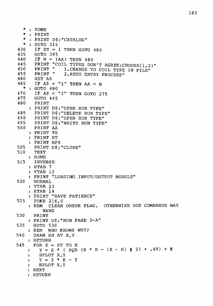
182
*: HOME
*: PRINT D$;
"CATALOG"
*: GOTO 315
430 IF ET = 1 THEN GOTO 480
435 GOTO 395
440 IF N = (AA) THEN 480
445 PRINT "COIL TYPES DON'T AGREE; CHOOSE ( 1 , 2 )"
450 PRINT"
1. CHANGE TO COIL TYPE IN FILE"
455 PRINT"
2. REDO ENTRY PROCESS"
460 GET A$
465 IF A$ ="1"
THEN AA = N*
: GOTO 480
470 IF A$ ="2"
THEN GOTO 275
475 GOTO 445
480 PRINT
: PRINT D$;"OPEN RUNTYPE"
485 PRINT D$; "DELETE RUNTYPE"
490 PRINT D$;"OPEN RUNTYPE"
495 PRINT D$; "WRITE RUNTYPE"
500 PRINT AA
: PRINT TS
: PRINT ET
: PRINT NF$
505 PRINT D$;"CLOSE"
510 TEXT
: HOME
515 INVERSE
: HTAB 7
: VTAB 12
: PRINT "LOADING INPUT/OUTPUTMODULE"
52 0 NORMAL
: VTAB 23
: HTAB 14
: PRINT "HAVEPATIENCE"
525 POKE 216,0
: REM CLEAR ONERR FLAG. OTHERWISE DOS COMMANDS MAY
HANG
530 PRINT
: PRINT D$;"RUN PAGE2-A"
535 GOTO 530
: REM WHO KNOWS WHY?
540 DRAW SH AT X,Y
: RETURN
545 FOR X = ST TO E
Y = S * ( SQR (R * R - (X -
H) t 2) + .49)+ K
HPLOT X,Y
Y = 2 * K - Y
HPLOT X,Y
NEXT
RETURN

183
PROGRAM LENGTH IS 3597 ($E0D) BYTES
A$
AA
B$
D$
DF$
E
ET
ET$
H
I
K
N
NF$
R
S
SH
ST
TS
TS$
X
Y
285
295
290
10,
495
320
160
370
370
160
175
160
340
315
160
160
250
160
310
310
175
250
295, 460, 465, 470
440, 465, 500
295
240, 325, 335, 345, 385, 395, 425, 480, 485, 490,505, 530
335,
170,
380,420
170,
325,
165,
375,
415,
165,
385, 395
215, 220, 225, 230, 545
385, 420, 425, 430, 500
215, 220, 230, 545
545
440, 465
320, 500
165, 215, 225, 545
545
255, 260, 265, 270, 540
165, 170, 220, 225, 230, 545
500
250, 255, 260, 265, 540, 545
255, 260, 265, 540, 545
APPENDIX C
PAGE 2-A PROGRAM MODULE
C.l Program Listing 185
C.2 Program Length and XRef 217
184
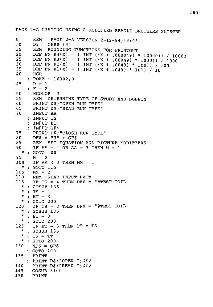
185
PAGE 2-A LISTING USING A MODIFIED BEAGLE BROTHERS XLISTER
5
10
15
20
25
30
35
40
45
50
55
60
65
70
75
80
85
90
*
95
100
105
110
115
*
*
*
120
*
*
*
125*
*
130
135
140
145
150
REM PAGE 2-A
D$ = CHR$ (4)
VERSION 2-12-84 ;14: 03
ROUNDING
FN R4(X)
R3(X)
R2(X)
Rl(X)
FN
FN
FN
= (= (= (= (
REM
DEF
DEF
DEF
DEF
HGR
POKE - 16302,0
D = 1
F = 2
HCOLOR= 3
REM DETERMINE
PRINT D$;"OPEN
PRINT D$
INPUT AA
INPUT TS
INPUT ET
INPUT GF$
PRINT D$; "CLOSE
DF$ ="@"
+ GF$
REM SET EQUATION
FUNCTIONS FOR
INT
INT
INT
INT
((X
((X
((X
((X
PRINTOUT
000049) *10000) ) / 10000
00049) *1000)) / 1000
0049) *100) ) / 100
049) *10) ) / 10
TYPE OF STUDY
RUNTYPE"
"READ RUNTYPE"
AND BOBBIN
RUNTYPE"
AND PICTURE MODIFIERS
IF AA = 1
GOTO 100
M = 2
IF AA < 3
GOTO 115
MM = 2
REM READ
IF TS = 4
GOSUB 135
TS = 1
ET = 3
GOTO 200
IF TS = 3
GOSUB 135
ET = 3
GOTO 200
IF ET = 3
GOSUB 135
TS = TT
GOTO 200
NF$ = GF$
GOTO 2 00
GOSUB
OR AA = 3 THEN M = 1
THEN MM = 1
INPUT DATA
THEN DF$ = "@TESTCOIL"
THEN DF$ = "@TESTCOIL"
THEN TT = TS
D$;"OPEN
D$;"READ
3100
"
;DF$
";DF$

186
: PRINT D$;"CLOSE"
155 NF$ = GF$
160 RETURN
198 REM BEGIN CREATING PICTURES
19 9 REM COMMON TO ALL
200 HPLOT 117,105 TO 117,50 TO 132,50 TO 132,105
: IF M = 1 THEN HPLOT TO 117,105
205 HPLOT 140,50 TO 135,50 TO 135,65 TO 140,65
210 HPLOT 140,30 TO 195,30 TO 195,85 TO 140,85 TO 140,30
215 HPLOT 150,30 TO 150,85
220 HPLOT 185,30 TO 185,85
225 HPLOT 195,50 TO 210,50 TO 210,105
: IF M = 1 THEN HPLOT TO 135,105 TO 135,90 TO 190,90
TO 195,85
230 HPLOT 20,0 TO 20,28
235 HPLOT 35,16 TO 35,47
240 HPLOT 41,16 TO 41,47
245 HPLOT 135,0 TO 135,48
250 HPLOT 140,0 TO 140,28
255 HPLOT 185,23 TO 185,28
260 HPLOT 195,23 TO 195,28
265 HPLOT 132,107 TO 132,120
270 IF M = 2 THEN 290
275 HPLOT 135,107 TO 135,120
280 HPLOT 67,105 TO 105,105
285 HPLOT 67,90 TO 105,90
290 SCALE= 1
: ROT= 0
: SH = 49
295 IF M = 1 THEN DRAW SH AT 102,90
300 DRAW SH AT 167,90
305 ROT= 32
310 DRAW SH AT 167,85
315 IF M = 2 THEN 330
320 DRAW SH AT 102,105
325 HPLOT 102,85 TO 102,105
330 ROT= 16
335 DRAW SH AT 135,5
340 DRAW SH AT 185,25
345 DRAW SH AT 132,115
350 DRAW SH AT 35,20
355 ROT= 48
360 DRAW SH AT 140,5
365 DRAW SH AT 195,25
370 DRAW SH AT 135,115
375 DRAW SH AT 41,20
380 HPLOT 135,5 TO 130,5
385 HPLOT 140,5 TO 145,5
390 HPLOT 185,25 TO 180,25
395 HPLOT 195,25 TO 200,25
400 HPLOT 132,115 TO 127,115
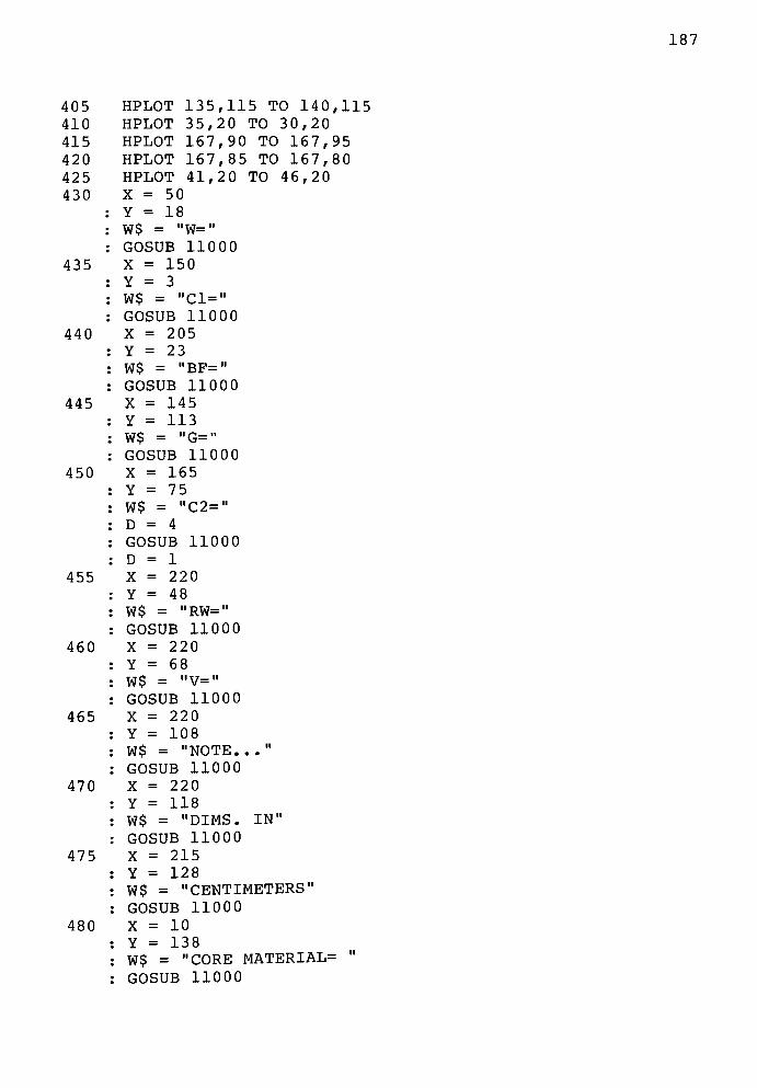
187
405
410
415
420
425
430
435
440
445
450
135,115 TO 140,115
35,20 TO 30,20
167,90 TO 167,95
167,85 TO 167,80
41,20 TO 46,20
455
460
465
470
475
480
HPLOT
HPLOT
HPLOT
HPLOT
HPLOT
X = 50
Y = 18
W$ =W="
GOSUB 11000
X = 150
Y = 3
W$ ="Cl="
GOSUB 11000
X = 205
Y = 23
W$ ="BF="
GOSUB 11000
X = 145
Y = 113
W$ ="G="
GOSUB 11000
X = 165
Y = 75
W$ ="C2="
D = 4
GOSUB 11000
D = 1
X = 220
Y = 48
W$ ="RW="
GOSUB 11000
X = 220
Y = 68
W$ =v="
GOSUB 11000
X = 220
Y = 108
W$ = "NOTE.
GOSUB 11000
X = 220
Y = 118
W$ = "DIMS.
GOSUB 11000
X = 215
Y = 128
W$ =
"CENTIMETERS"
GOSUB 11000
X = 10
Y = 138
W$ = "COREMATERIAL^
"
GOSUB 11000
IN"

188
485 X = (139 - ( LEN (NF$)) *3)
: Y = 168
: W$ = NF$
: GOSUB 11000
490 X - 57
: Y = 153
: W$ = "D.C. HORSESHOE ELECTROMAGNET"
: GOSUB 11000
495 IF M = 1 THEN 550
500 HPLOT 140,105 TO 140,90 TO 195,90 TO 195,85 TO 195,105505 HPLOT 150,105 TO 150,90
510 HPLOT 185,105 TO 185,90
515 HPLOT 135,120 TO 135,67
520 HPLOT 67,50 TO 92,50
525 HPLOT 67,65 TO 92,65
530 HPLOT 89,50 TO 89,90 TO 102,90 TO 102,85
535 SH = 49
540 ROT= 32
: DRAW SH AT 89,65
545 ROT= 0
: DRAW SH AT 89,50
550 ON MM GOTO 560,665
555 REM COMMON TO DES&ANAL SQ560 HPLOT 20,30 TO 85,30 TO 85,85 TO 20,85 TO 20,30
565 HPLOT 41,50 TO 64,50 TO 64,65 TO 41,65 TO 41,50
570 HPLOT 41,44 TO 64,44 TO 70,50 TO 70,65 TO 64,71 TO 41,
71 TO 35,65 TO 35,50 TO 41,44
575 HPLOT 41,107 TO 41,125
580 HPLOT 64,107 TO 64,125
585 SH = 49
590 ROT= 48
: DRAW SH AT 41,115
595 ROT= 16
: DRAW SH AT 64,115
600 HPLOT 64,115 TO 36,115
605 IF M = 2 THEN 630
610 HPLOT 41,90 TO 64,90 TO 64,105 TO 41,105 TO 41,90
615 ROT= 56
: DRAW SH AT 64,105
620 HPLOT 64,105 TO 75,116 TO 80,116
625 GOTO 655
630 ROT= 56
: DRAW SH AT 64,65
635 HPLOT 64,65 TO 75,76 TO 75,116 TO 80,116
640 HPLOT 20,105 TO 20,90 TO 85,90 TO 85,105
645 HPLOT 41,107 TO 41,67
650 HPLOT 64,107 TO 64,67
655 ON TS GOSUB 1130,820,1130
657 POKE - 16301,0
660 ON TS GOTO 1300,1345,1400
665 REM COMMON TO DES&ANAL RND
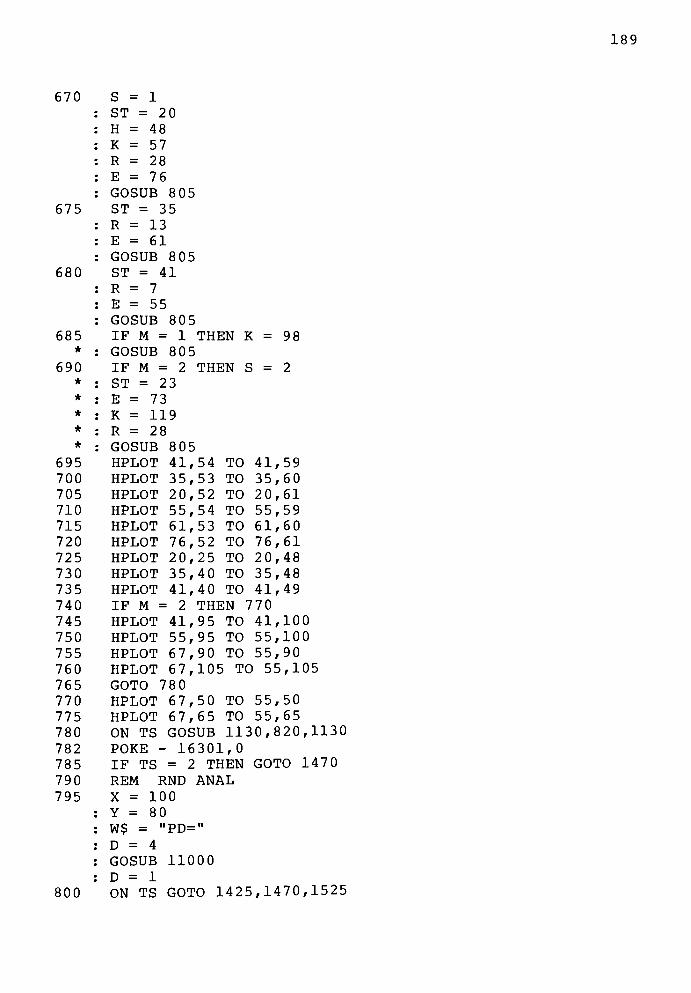
189
670 S = 1
ST = 20
H = 48
K = 57
R = 28
E = 76
GOSUB 8 05
675 ST = 35
: R = 13
: E = 61
: GOSUB 8 05
680 ST = 41
: R = 7
: E = 55
: GOSUB 8 05
68 5 IF M = 1 THEN K = 98*
: GOSUB 805
690 IF M = 2 THEN S = 2
*: ST = 23
*: E = 73
*: K = 119
*: R = 28
*: GOSUB 805
695 HPLOT 41,54 TO 41,59
700 HPLOT 35,53 TO 35,60
705 HPLOT 20,52 TO 20,61
710 HPLOT 55,54 TO 55,59
715 HPLOT 61,53 TO 61,60
720 HPLOT 76,52 TO 76,61
725 HPLOT 20,25 TO 20,48
730 HPLOT 35,40 TO 35,48
735 HPLOT 41,40 TO 41,49
740 IF M = 2 THEN 770
745 HPLOT 41,95 TO 41,100
750 HPLOT 55,95 TO 55,100
755 HPLOT 67,90 TO 55,90
760 HPLOT 67,105 TO 55,105
765 GOTO 780
770 HPLOT 67,50 TO 55,50
775 HPLOT 67,65 TO 55,65
780 ON TS GOSUB 1130,820,1130
782 POKE - 16301,0
785 IF TS = 2 THEN GOTO 1470
79 0 REM RND ANAL
795 X = 100
Y = 80
W$ ="PD="
D = 4
GOSUB 11000
D = 1
800 ON TS GOTO 1425,1470,1525

190
815
820
825
830
835
840
HPLOT 0,105 TO 39,105
HPLOT 10,105 TO 10,90
SH = 49
8 05 FOR X = ST TO E
: Y = ( SQR (R * R +.0001
- (X -
H) i 2) +.49) + K
: IF S - 1 THEN HPLOT X,Y
810 Y = 2 * K - Y
: HPLOT X,Y
: NEXT
RETURN
REM COMMON SING DES REQHPLOT 18,30 TO 0,30
HPLOT 10,30 TO 10,45
HPLOT 20,10 TO 25,10
HPLOT 117,107 TO 117,111
oiu HPLOT 117,120 TO 117,135
845 HPLOT 210,107 TO 210,135
850 HPLOT 117,127 TO 140,127
855 HPLOT 187,127 TO 210,127
860 HPLOT 93,82 TO 93,85 TO 111,85 TO 111,82
865 HPLOT 18,48 TO IP A c mri n Ac n "
870 HPLOT 184,136 TO
875 HPLOT 143,136 TO
880 HPLOT 28,18 TO
885 HPLOT 18,87 TO
890 IF M = 2 THEN 910
895
900
905 SH = 49
: ROT= 3 2
: DRAW SH AT 10,105
910 SH = 49
: ROT= 48
: DRAW SH AT 20,10
915 DRAW SH AT 117,127
920 ROT= 16
: DRAW SH AT 210,127
925 ROT= 0
: DRAW SH AT 10,30
930 X = 30
: Y = 4
: W$ ="DX="
: GOSUB 11000
935 X = 30
: Y = 11
: W$ ="DN="
: GOSUB 11000
940 X = 220
: Y = 32
: W$ ="GX=#"
: GOSUB 11000
945 X = 220
: Y = 38
: W$ ="GN=#"

191
: GOSUB 11000
950 X = 220
: Y = 58
: W$ ="IX="
: GOSUB 11000
955 X = 220
: Y = 78
: W$ ="BX="
: GOSUB 11000
960 X = 220
: Y = 88
: W$ ="HX="
: GOSUB 11000
965 X = 220
: Y = 98
: W$ ="HN="
: GOSUB 11000
970 X = 145
: Y = 121
: W$ ="LX="
: GOSUB 11000
975 X = 145
: Y = 128
: W$ ="LN="
: GOSUB 11000
980 X = 4
Y = 85
W$ ="WX="
D = 4
GOSUB 11000
985 X = 11
Y = 85
W$ ="WN="
GOSUB 11000
D = 1
990 IF MM = 2 THEN GOTO 1070
995 REM SQ DES REQ
1000 HPLOT 80,10 TO 85,10
1005 HPLOT 85,0 TO 85,16
1010 HPLOT 85,24 TO 85,28
1015 HPLOT 80,16 TO 80,1 TO 77,1
1020 HPLOT 3,106 TO 0,106 TO 0,132
1025 ROT= 16
: DRAW 49 AT 85,10
: ROT= 0
1030 X = 5
Y = 108
W$ ="XD/ND="
GOSUB 11000
1035 X = 96
; Y = 80
TO 3,132
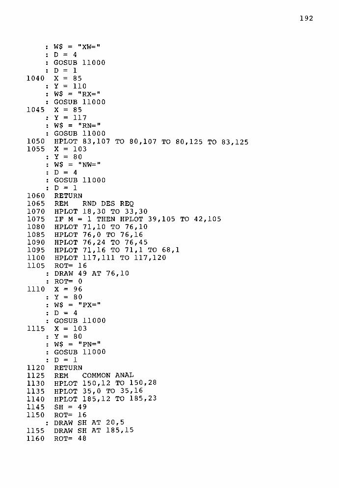
192
W$ ="XW="
D = 4
GOSUB 11000
D - 1
1040 X = 85
: Y = 110
: W$ ="RX="
: GOSUB 11000
1045 X - 85
: Y = 117
: W$ ="RN="
: GOSUB 11000
1050 HPLOT 83,107 TO 80,107 TO 80,125 TO 83,125
1055 X = 103
Y = 80
W$ ="NW="
D = 4
GOSUB 11000
D = 1
1060 RETURN
1065 REM RND DES REQ
1070 HPLOT 18,30 TO 33,30
1075 IF M = 1 THEN HPLOT 39,105 TO 42,105
1080 HPLOT 71,10 TO 76,10
1085 HPLOT 76,0 TO 76,16
1090 HPLOT 76,24 TO 76,45
1095 HPLOT 71,16 TO 71,1 TO 68,1
1100 HPLOT 117,111 TO 117,120
1105 ROT= 16
: DRAW 49 AT 76,10
: ROT= 0
1110 X = 96
Y = 80
W$ ="PX="
D = 4
GOSUB 11000
1115 X = 103
Y = 80
W$ ="PN="
GOSUB 11000
D = 1
1120 RETURN
1125 REM COMMON ANAL
1130 HPLOT 150,12 TO 150,28
1135 HPLOT 35,0 TO 35,16
1140 HPLOT 185,12 TO 185,23
1145 SH = 49
1150 ROT= 16
: DRAW SH AT 2 0,5
1155 DRAW SH AT 185,15
1160 ROT= 48

193
: DRAW SH AT 35,5
1165 DRAW SH AT 150,151170 HPLOT 20,5 TO 15,5
1175 HPLOT 35,5 TO 4 0,5
1180 HPLOT 190,15 TO 150,151185 X = 45
: Y = 3
: W$ ="FW="
: GOSUB 11000
1190 X = 195
: Y = 13
: W$ ="LW="
: GOSUB 11000
1195 X = 220
: Y = 38
: W$ ="WG=#"
: GOSUB 11000
1200 X = 220
: Y = 58
: W$ ="N="
: GOSUB 11000
1205 IF MM = 2 THEN RETURN
1210 REM SQ ANAL
1215 X = 5
: Y = 108
: W$ ="CD="
: GOSUB 11000
1220 X = 100
: Y = 80
: W$ ="CW="
: D = 4
: GOSUB 11000
D = 1
1225 X = 85
Y = 114
W$ ="R="
GOSUB 11000
1230 RETURN
1298 REM PRINTING ROUTINE CALLS FOLLOW
1299 REM PRINT FOR SQ ANAL INPUT
1300 HOME
VTAB 24
1305 IF ET = 3 THEN GOTO 1325
1310 GOSUB 1800
GOSUB 1810
GOSUB 1820
GOSUB 1830
GOSUB 1840
GOSUB 18 5 0
GOSUB 1860
GOSUB 18 85
194
: GOSUB 1895
1315 GOSUB 1905
GOSUB 1920
GOSUB 1955
GOSUB 1970
GOSUB 20 05
GOSUB 202 5
1320 GOTO 2105
1325 GOSUB 1805
GOSUB 1815
GOSUB 1825
GOSUB 183 5
GOSUB 1845
GOSUB 1855
GOSUB 1880
GOSUB 189 0
GOSUB 19 0 0
1330 GOSUB 1915
GOSUB 1925
GOSUB 196 5
GOSUB 1975
GOSUB 2010
GOSUB 2 03 0
1335 GOTO 2105
1340 REM PRINT FOR SQ DES INPUT
1345 HOME
: VTAB 24
1350 IF ET = 3 THEN GOTO 1375
1355 GOSUB 1670
GOSUB 1680
GOSUB 1695
GOSUB 1705
GOSUB 172 0
GOSUB 173 0
GOSUB 1745
GOSUB 1755
GOSUB 177 0
GOSUB 1780
GOSUB 17 9 0
1360 GOSUB 1810
GOSUB 1820
GOSUB 1840
GOSUB 1860
GOSUB 1895
GOSUB 1905
GOSUB 1930
GOSUB 1940
GOSUB 1980
GOSUB 19 90
GOSUB 2 0 05
GOSUB 2025
195
1365
1370
1375
1380
1385
1390
1395
1400
1405
1410
GOSUB 1640
GOSUB 1600
GOSUB 1620
GOTO 2105
GOSUB 1675
GOSUB
GOSUB
GOSUB
GOSUB
GOSUB
GOSUB
GOSUB
GOSUB
GOSUB
GOSUB
GOSUB
GOSUB
GOSUB
GOSUB
GOSUB
GOSUB
GOSUB
GOSUB
GOSUB
GOSUB
GOSUB
GOSUB
GOSUB
GOSUB
GOSUB
GOTO
1690
1700
1715
1725
1740
1750
1765
1775
1785
1795
1815
1825
1845
1865
1900
1915
1935
1950
1985
2000
2010
2030
1660
1615
1635
2105
REM PRINT
HOME
VTAB 24
GOSUB 1805
GOSUB
GOSUB
GOSUB
GOSUB
GOSUB
GOSUB
GOSUB
1415
1420
GOSUB
GOSUB
GOSUB
GOSUB
GOSUB
GOSUB
GOSUB
GOTO
1815
1825
1835
1845
1855
1880
1890
1900
1915
1925
1965
1975
2010
2030
2105
FOR SQ DES OUTPUT
REM PRINT FOR RND ANAL INPUT
196
1425
1430
1435
HOME
VTAB 24
1440
1445
1450
1455
1460
1465
1470
1475
1480
1485
IF ET
GOSUB
GOSUB
GOSUB
GOSUB
GOSUB
GOSUB
GOSUB
GOSUB
GOSUB
GOSUB
GOSUB
GOSUB
GOSUB
GOTO
GOSUB
GOSUB
GOSUB
GOSUB
GOSUB
GOSUB
GOSUB
GOSUB
GOSUB
GOSUB
GOSUB
GOSUB
GOSUB
GOTO
= 3 THEN
1800
1810
1820
1830
1840
1850
1860
1885
1895
1905
2005
2025
2035
2105
1805
1815
1825
1835
1845
1855
1880
1890
1900
1915
2010
2030
2040
2105
GOTO 1450
REM PRINT FOR RND DES INPUT
HOME
VTAB 24
IF ET
GOSUB
GOSUB
GOSUB
GOSUB
GOSUB
GOSUB
GOSUB
GOSUB
GOSUB
GOSUB
GOSUB
GOSUB
GOSUB
GOSUB
GOSUB
GOSUB
= 3 THEN
1695
1705
1720
1730
1745
1755
1770
1780
1790
1810
1820
1840
1860
1895
1905
2005
GOTO 1500
197
1490
1495
1500
1505
1510
1515
1520
1525
1535
1540
1599
1600
1605
*
GOSUB 202 5
GOSUB 20 4 5
GOSUB 2055
GOSUB 1640
GOSUB 1600
GOSUB 1620
GOTO 2105
GOSUB 1700
GOSUB
GOSUB
GOSUB
GOSUB
GOSUB
GOSUB
GOSUB
GOSUB
GOSUB
GOSUB
GOSUB
GOSUB
GOSUB
GOSUB
GOSUB
GOSUB
GOSUB
GOSUB
GOSUB
GOSUB
GOSUB
GOTO
1715
1725
1740
1750
1765
1775
1785
1795
1815
1825
1845
1880
1900
1915
2010
2030
2050
2065
1660
1615
1635
2105
REM PRINT
HOME
VTAB 24
FOR RND DES OUTPUT
1530 GOSUB 1805
1815
1825
1835
1845
1855
1880
1890
1900
1915
2010
2030
2040
GOSUB
GOSUB
GOSUB
GOSUB
GOSUB
GOSUB
GOSUB
GOSUB
GOSUB
GOSUB
GOSUB
GOSUB
GOTO 2105
REM INPUT STATEMENTS FOLLOW
INPUT "ENTER MAX INDUCTANCE ( HENRIES ), HX= (RETURN=5 )
IF A$ =""
THEN HX = 5
GOTO 1615
;A$
198
1610 HX = VAL (A$)
1615 X = 238
Y = 88
A = FN R2(HX)
W$ = STR$ (A)
GOSUB 11000
RETURN
1620 INPUT "ENTER MIN INDUCTANCE ( HENRIES ), HN= (RETURN=0):"
;A$
1625 IF A$ =""
THEN HN = 0*
: GOTO 1635
1630 HN = VAL (A$)
1635 X = 238
Y = 98
A = FN R2(HN)
W$ = STR$ (A)
GOSUB 11000
RETURN
INPUT "ENTER MAX FLUX DENSITY (KILOGAUSSES ), BX= (DEFAULT
=B.SAT) :";BX$
BX = VAL (BX$)
IF BX$ =""
THEN BX = 0
X = 238
Y = 78
W$ ="BSAT"
GOSUB 11000
RETURN
IF BX > 20 THEN PRINT "BX MUST BE<=20"
GOTO 1640
X = 238
Y = 78
A = FN R2(BX)
W$ = STR$ (A)
IF BX = 0 THEN W$ ="BSAT"
1665 GOSUB 11000
: RETURN
167 0 INPUT "ENTER MAX CORNER RAD ,RX= "
; RX
1675 X = 103
Y = 110
A = FN R2(RX)
W$ = STR$ (A)
GOSUB 11000
RETURN
168 0 INPUT "ENTER MIN CORNER RAD,RN= (RETURN=0 )"
;A$
: IF A$ =""
THEN RN = 0
*: GOTO 1690
1685 RN = VAL (A$)
1690 X = 103
Y = 117
A = FN R2(RN)
W$ = STR$ (A)
GOSUB 11000
1640
1645
1650
*
*
*
*
*
1655*
1660
199
: RETURN
1695 INPUT "ENTER
1700 X = 48
Y = 4
A = FN R2(DX)
W$ = STR$ (A)GOSUB 11000
RETURN
1705
*
1710
1715
1720
1725
1730
*
1735
1740
1745
1750
1755
*
1760
1765
MAX OVERALL DEPTH,DX="
;DX
J\ril"UKlN
INPUT "ENTER MIN OVERALL DEPTH, DN= (RETURN=0 )" -ASIF A$ =
""
THEN DN = 0
GOTO 1715
DN = VAL (A$)X = 48
Y = 11
A = FN R2(DN)
W$ = STR$ (A)GOSUB 11000
RETURN
INPUT "ENTER MAX OVERALL WIDTH,WX="
;WX
X = 4
Y = 67
A = FN R2(WX)
W$ = STR$ (A)D = 4
GOSUB 11000
D = 1
RETURN
INPUT "ENTER MIN OVERALL WIDTH,WN= (RETURN=0)"
;A$
IF A$ =""
THEN WN = 0
GOTO 17 4 0
WN = VAL (A$)X = 11
Y = 67
A = FN R2(WN)
W$ = STR$ (A)
D = 4
GOSUB 11000
D = 1
RETURN
INPUT "ENTER MAX OVERALL LENGTH, LX=";LX
X = 163
Y = 121
A = FN R2(LX)
W$ = STR$(" '
GOSUB 11000
RETURN
INPUT "ENTER
IF A$ ="
GOTO 1765
LN = VAL (A$)
X = 163
(A)
._. MIN OVERALL LENGTH, LN= (RETURN=0)"
;A$
THEN LN = 0
200
1770
1775
1780
1785
1790
*
1795
1800
1805
1810
1815
1820
1825
1830
Y = 128
A = FN R2(LN)
W$ = STR$ (A)GOSUB 11000
RETURN
INPUT "ENTER MAX CURRENT (AMPS ) ,IX="
IXX = 238
Y = 58
A = FN R2(IX)
W$ = STR$ (A)GOSUB 11000
RETURN
INPUT "ENTER MAX WIRE GAGE NO. -GX
X = 244
Y = 32
A = FN Rl(GX)
W$ = STR$ (A)GOSUB 11000
RETURN
INPUT "ENTER MIN WIRE GAGE NO.,GN=";GNIF GN = 0 THEN PRINT "GN MUST BE
>0"
GOTO 17 9 0
X = 244
Y = 38
A = FN Rl(GN)
W$ = STR$ (A)GOSUB 11000
RETURN
VTAB 24
INPUT "ENTER FLANGE WIDTH,FW='
X = 63
Y = 3
A = FN R3(FW)
W$ = STR$ (A)GOSUB 11000
RETURN
INPUT "ENTER WALL THICKNESS,W="
X = 62
Y = 18
A = FN R3(W)
W$ = STR$ (A)
GOSUB 11000
RETURN
INPUT "ENTER ARMATURE CLEARANCE, C1= ";CI
X = 168
Y = 3
A = FN R3(C1)
W$ = STR$ (A)
GOSUB 11000
RETURN
INPUT "ENTER WINDING LENGTH,LW="
;LW
FW
;W
201
1835
1840
1845
1850
1855
1860
1865
1870
*
1875*
1880
1885
1890
1895
1900
1905
*
1910
1915
WIND FACTOR (RETURN=1 ) ,RW="
;RW$
RW
X = 213
Y = 13
A = FN R3(LW)
W$ = STR$ (A)
GOSUB 11000
RETURN
INPUT "ENTER BOBBIN FLANGE THICKNESS ;BF
X = 223
Y = 23
A = FN R3(BF)
W$ = STR$ (A)
GOSUB 11000
RETURN
INPUT "WIRE GAGE NUMBER,WG="
;WG
X = 244
Y = 38
A = FN Rl(WG)
W$ = STR$ (A)GOSUB 11000
RETURN
INPUT "RANDOM
RW = VAL (RW$)
IF RW$ =""
THEN
GOTO 1880
IF RW > 1 THEN PRINT "RW MUST BE<=1"
GOTO 1860
X = 238
Y = 48
A = FN R3(RW)
W$ = STR$ (A)
GOSUB 11000
RETURN
INPUT "NUMBER OF TURNS,N=";N
X = 232
Y = 58
A = FN R1(N)
W$ = STR$ (A)
GOSUB 11000
RETURN
INPUT "OPERATING VOLTAGE ,V= "; V
X = 232
Y = 68
A = FN R3(V)
W$ = STR$ (A)
GOSUB 11000
RETURN
INPUT "AIR
IF A$ =""
GOTO 1915
G = VAL (A$)
X = 157
GAP ( PER
THEN G =.002
POLE ) , G= ( RET= . 0 0 2 )"
;A$
202
Y = 113
A = FN R4(G)
W$ = STR$ (A)
GOSUB 11000
: RETURN
1920 INPUT "CORE DEPTH,CD="
;CD
1925 X = 5
Y = 118
A = FN R3(CD)
W$ = STR$ (A)
GOSUB 11000
1930
1935
RETURN
INPUT "ENTER MAX CORE DEPTH, XD=";XD
X = 5V 11/1Y = 114
A = FN R3(XD)
W$ = STR$ (A)
GOSUB 11000
: RETURN
1940 INPUT "ENTER MIN CORE DEPTH, ND= (RETURN=0)"
;A$
: IF A$ =""
THEN ND = 0
*: GOTO 1950
1945 ND = VAL (A$)
1950 X = 5
Y = 120
A = FN R3(ND)
W$ = STR$ (A)
GOSUB 11000
: RETURN
1955 INPUT "CORE RADIUS, R= (RETURN=0)"
;A$
: IF A$ =""
THEN R = 0
*: GOTO 1965
1960 R = VAL (A$)
1965 X = 97
Y = 114
A = FN R3(R)
W$ = STR$ (A)
.GOSUB 11000
: RETURN
1970 INPUT "CORE WIDTH,CW="
;CW
1975 X = 100
Y = 62
A = FN R3(CW)
W$ = STR$ (A)
D = 4
GOSUB 11000
D = 1
: RETURN
1980 INPUT "ENTER MAX CORE WIDTH, XW=";XW
1985 X = 96
: Y = 62
203
1990
*
1995
2000
2005
2010
2015
2020
2025
2030
2035
2040
2045
2050
A = FN R3(XW)
W$ = STR$ (A)D = 4
GOSUB 11000
D = 1
RETURN
INPUT "ENTER MIN CORE WIDTH, NW= (RETURN=0 )" -A$IF A$ =
""
THEN NW = 0
GOTO 2000
NW = VAL (A$)X = 103
Y = 62
A = FN R3(NW)
W$ = STR$ (A)D = 4
GOSUB 11000
D = 1
RETURN
INPUT "CORE MATERIAL=";CM$X = 94
Y = 138
W$ = CM$
GOSUB 11000
IF LEFT$ (CM$,1) = CHR$ (93) THEN CM$ = RIGHT$ (CM$,( LEN (CM$) - 1) )
DM$ = CHR$ (93) + CM$
RETURN
INPUT "CORE CLEARANCE,C2=";C2X = 165
Y = 57
D = 4
A = FN R3(C2)
W$ = STR$ (A)GOSUB 11000
D = 1
RETURN
INPUT "POLE DIA.,PD=";PD
X = 100
Y = 62
A = FN R3(PD)
W$ = STR$ (A)
D = 4
GOSUB 11000
D = 1
RETURN
INPUT "ENTER MAX POLE DIA.,PX=";PX
RX = PX / 2
X = 96
Y = 62
A = FN R3(PX)
W$ = STR$ (A)
204
D = 4
GOSUB 11000
D = 1
RETURN
2055 INPUT "ENTER MIN POLE DIA. , PN= ( RETURN=0 )"
;A$: IF A$ =
""
THEN PN = 0*
: RN = 0
*: GOTO 2 06 5
2060 PN = VAL (A$)
: RN = PN / 2
2065 X = 103
Y = 62
A = FN R3(PN)
W$ = STR$ (A)D = 4
GOSUB 11000
D = 1
RETURN
2100 REM BEGIN CHANGES SEQUENCE
2105 PRINT "DO YOU WISH TO CHANGE ANY VALUES? (Y/N) :"
: GET A$
2110 IF A$ ="Y"
THEN FL = 1
*: GOTO 2125
2115 IF A$ < >"N"
THEN 2105
2120 GOTO 2500
2125 IF TS = 3 THEN TS = 1
2130 INPUT "ENTER ONE VARIABLE ID:";A$
2135 REM COMMON TO ALL
2140 D = 1
2145 IF A$ ="W"
THEN HOME
*: GOSUB 1815
*: VTAB 24
*: PRINT "CURRENT W=";W
*: GOSUB 1810
*: GOTO 2105
215 0 IF A$ ="CI"
THEN HOME
*: GOSUB 1825
*: VTAB 24
*: PRINT "CURRENT
Cl="
;Cl
*: GOSUB 1820
*: GOTO 2105
2155 IF A$ ="BF"
THEN HOME
*: GOSUB 1845
*: VTAB 24
*: PRINT "CURRENT BF=";BF
*: GOSUB 1840
*: GOTO 2105
2160 IF A$ ="RW"
THEN HOME
*: GOSUB 1880
*: VTAB 24
*: PRINT "CURRENT RW=";RW
205
*: GOSUB 1860
*: GOTO 2105
2165 IF A$ ="V"
THEN HOME*
: GOSUB 1900*
: VTAB 24
*: PRINT "CURRENT V=";V
*: GOSUB 1895
*: GOTO 2105
2170 IF A$ ="G"
THEN HOME*
: GOSUB 1915*
: VTAB 24*
: PRINT "CURRENTG="
;G
*: GOSUB 1905
*: GOTO 2105
2175 IF LEFT$ (A$,2) ="CM"
OR A$ = "CORE MATERIAL"
THEN
HOME
*: GOSUB 2010
*: VTAB 24
*: PRINT "CURRENT CM$=";CM$
*: GOSUB 2005
*: GOTO 2105
2180 IF A$ ="C2"
THEN HOME
*: D = 4
*: GOSUB 2030
*: VTAB 24
*: PRINT "CURRENT
C2="
;C2
*: GOSUB 2 025
*: D = 1
*: GOTO 2105
2185 ON AA GOTO 2190,2190,2195,2195
2190 IF A$ ="R"
THEN HOME
*: GOSUB 1965
*: VTAB 24
*: PRINT "CURRENT R=";R
*: GOSUB 1955
* . GOTO 2105
2195 ON TS GOTO 2275,2205,2275
2200 REM COMMON TO ALL DESIGN
2205 IF A$ ="DX"
THEN HOME
*: GOSUB 1700
* . VTAB 24
*: PRINT "CURRENT DX=";DX
*: GOSUB 1695
*: GOTO 2105
2210 IF A$ ="DN"
THEN HOME
*: GOSUB 1715
* . VTAB 24
*: PRINT "CURRENT DN=";DN
* . GOSUB 1705
*: GOTO 2105
2215 IF A$ ="WX"
THEN HOME
206
*: GOSUB 1725
*: VTAB 24
*: PRINT "CURRENT WX=";WX
*: GOSUB 1720
*: GOTO 2105
222 0 IF A$ ="WN"
THEN HOME*
: GOSUB 1740*
: VTAB 24*
: PRINT "CURRENT WN=";WN*
: GOSUB 1730*
: GOTO 2105
2225 IF A$ ="LX"
THEN HOME*
: GOSUB 1750*
: VTAB 24
*: PRINT "CURRENT LX=";LX
*: GOSUB 1745
*: GOTO 2105
223 0 IF A$ ="LN"
THEN HOME
*: GOSUB 1765
*: VTAB 24
*: PRINT "CURRENT LN=";LN
*: GOSUB 1755
*: GOTO 2105
2235 IF A$ ="BX"
THEN HOME
*: GOSUB 1785
*: VTAB 24
*: PRINT "CURRENT BX=";BX
*: GOSUB 1780
*: GOTO 2105
224 0 IF A$ ="IX"
THEN HOME
*: GOSUB 1775
*: VTAB 24
*: PRINT "CURRENT IX=";IX
*: GOSUB 1770
*: GOTO 2105
2245 IF A$ ="GX"
THEN HOME
*: GOSUB 1785
*: VTAB 24
*: PRINT "CURRENT GX=";GX
*: GOSUB 1780
*: GOTO 2105
2250 IF A$ ="GN"
THEN HOME
*: GOSUB 1795
*: VTAB 24
*: PRINT "CURRENT GN=";GN
*: GOSUB 1790
*: GOTO 2105
2255 IF A$ ="HX"
THEN HOME
*: GOSUB 1615
*: VTAB 24
*: PRINT "CURRENT HX=";HX
207
*: GOSUB 1600
*: GOTO 2105
2260 IF A$ ="HN"
THEN HOME*
: GOSUB 1635*
: VTAB 24
*: PRINT "CURRENT HN=";HN
*: GOSUB 1620
*: GOTO 2105
2265 ON AA GOTO 2305,2305,2345,23452270 REM COMMON TO ALL ANAL
2275 IF A$ ="FW"
THEN HOME*
: GOSUB 1805*
: VTAB 24*
: PRINT "CURRENT FW=";FW
*: GOSUB 1800
*: GOTO 2105
2280 IF A$ ="LW"
THEN HOME
*: GOSUB 1835
*: VTAB 24
*: PRINT "CURRENT LW=";LW
*: GOSUB 1830
*: GOTO 2105
2285 IF A$ ="WG"
THEN HOME
*: GOSUB 1855
*: VTAB 24
*: PRINT "CURRENT WG=";WG
*: GOSUB 1850
*: GOTO 2105
2290 IF A$ ="N"
THEN HOME
*: GOSUB 1890
*: VTAB 24
*: PRINT "CURRENT N=";N
*: GOSUB 1885
*: GOTO 2105
2295 ON AA GOTO 2365,2365,2385,2385
2300 REM SQ DES
23 05 IF A$ ="XD"
THEN HOME
*: GOSUB 1935
*: VTAB 24
*: PRINT "CURRENT XD=";XD
*: GOSUB 1930
*: GOTO 2105
2310 IF A$ ="ND"
THEN HOME
*: GOSUB 1950
*: VTAB 24
*: PRINT "CURRENT ND=";ND
*: GOSUB 1940
*: GOTO 2105
2315 IF A$ ="XW"
THEN HOME
*: GOSUB 1985
*: VTAB 24
208
*: PRINT "CURRENT XW=";XW
*: GOSUB 1980
*: GOTO 2105
2320 IF A$ ="NW"
THEN HOME*
: GOSUB 2000*
: VTAB 24*
: PRINT "CURRENT NW=";NW*
: GOSUB 1990*
: GOTO 2105
2325 IF A$ ="RX"
THEN HOME*
: GOSUB 1675*
: VTAB 24*
: PRINT "CURRENT RX=";RX*
: GOSUB 1670*
: GOTO 2105
2330 IF A$ ="RN"
THEN HOME*
: GOSUB 1690*
: VTAB 24*
: PRINT "CURRENT RN=";RN*
: GOSUB 1680*
: GOTO 2105
2335 GOTO 2105
2340 REM RND DES
2345 IF A$ ="PX"
THEN HOME
*: GOSUB 2050
*: VTAB 24
*: PRINT "CURRENT PX=";PX
*: GOSUB 2045
*: GOTO 2105
2350 IF A$ ="PN"
THEN HOME
*: GOSUB 2065
*: VTAB 24
*: PRINT "CURRENT PN=";PN
*: GOSUB 2055
*: GOTO 2105
2355 GOTO 2105
2360 REM SING SQ ANAL
2365 IF A$ ="CD"
THEN HOME
*: GOSUB 1925
*: VTAB 24
*: PRINT "CURRENT CD=";CD
*: GOSUB 1920
*: GOTO 2105
2370 IF A$ ="CW"
THEN HOME
*: GOSUB 1975
*: VTAB 24
*: PRINT "CURRENT CW=";CW
*: GOSUB 1970
*: GOTO 2105
2375 GOTO 2105
2380 REM RND ANAL

209
2385*
*
*
*
*
2390
2499
2500
2505
2510
2515
2520
2525
2530
2535
2540
2545
2550
2555
2560
2565
2570
2575
2580
2585
2590
2595
2600
2605
IF A$ ="PD"
THEN HOME
GOSUB 2040
VTAB 24
PRINT "CURRENT PD=";PD
GOSUB 2035
GOTO 2105
GOTO 2105
REM OUTPUT OPTIONS
HOME
TEXT
PRINT "CHOOSE ONE(1-5):"
HTAB 5
PRINT "1. PRINT OUT COIL INFORMATION"
HTAB 5
PRINT "2. SAVE COIL INFORMATION TODISK"
HTAB 5
PRINT "3.MAKE MORECHANGES"
ON TS GOTO 2530,2540,2530
HTAB 5
PRINT "4. PERFORMANALYSIS"
GOTO 2545
HTAB 5
PRINT "4. BEGIN NEWDESIGN"
HTAB 5
PRINT "5.QUIT"
GET A$
A = VAL (A$)
ON A GOTO 2565,2580,2730,2750,3245
ON A GOTO 2500,2500,2105,3035,3245
INVERSE
PRINT "BE SURE PRINTER IS TURNEDON"
NORMAL
PRINT "HIT RETURN WHENREADY"
GET A$
PRINTD$;"PR#1"
PRINT CHR$ (9);"G"
PRINTD$;"PR#0"
GOTO 2560
ONERR GOTO 264 0
ET = 3
DF$ ="@"
+ NF$
PRINT D$;"OPEN ";DF$
PRINT D$;"READ ";DF$
INPUT AN
INPUT BN
INPUT CN
210
2610
2615
2620
2625
2630
2635
2640
2645
2650
2655
2660
2665
2670
2675
2680
2685
2690
2695
2700*
*
2705
2710
2715
2720
2725
2730
2735
2740
2745
2750
2755
2760
2765
2770
2775
2780
2785
2790*
2795*
"CLOSE"
PRINT D$;"CLOSE"
PRINT "FILE ALREADY EXISTS. CHOOSE (1-2)PRINT
"
1. OVERWRITE EXISTING FILE"
PRINT"
2. RENAME NEWFILE"
GET A$
IF A$ ="1"
THEN 2645
IF A$ ="2"
THEN 2690
GOTO 2615
PRINT D$
POKE 216,0
GOSUB
REM
PRINT D$;"CLOSE"
GOTO 2560
PRINT "DO YOU WANT TO REVIEW THE CATALOG ( Y/N )"
GET A$
IF A$ ="Y"
THEN PRINT
PRINTD$;"CATALOG"
GOTO 2710
IF A$ < >"N"
THEN GOTO 2690
INPUT "ENTER FILENAME:"
;NF$
IF LEFT$ (NF$,1) =""
THEN NF$ = RIGHT$ (NF$,( LEN
(NF$) - 1))
DF$ ="@"
+ NF$
GOTO 2580
D$
D$
D$
D$
3200
"OPEN ";DF$
"DELETE ";DF$"OPEN ";DF$
"WRITE ";DF$
DF$ =
POKE
POKE
POKE
POKE
HOME
VTAB
GOTO
DM$ =
ONERR
INPUT
POKE
IF TS
'@TESTCOIL"
16304,0
16297,0
16300,0
16301,0
24
2560
CHR$ (93)
GOTO 2975
D$;"OPEN
"READ
+ CM$
";DM$
";DM$D$
BB
D$;"CLOSE"
216,0
< > 2 THEN GOTO
IF DX < DN THEN PRINT
GOTO 2505
IF LX < LN THEN
GOTO 2505
2950
"DX MUST BE >DN"
PRINT "LX MUST BE >LN"
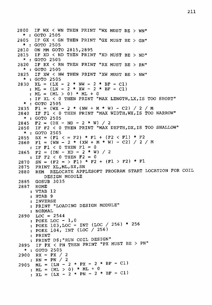
211
2800
2805
2810
2815
*
2820
*
2825
*
2830
2835
2840
*
2845
2850
*
2855
2860
2865
2870
2875
2880
2885
2887
2890
2895
*
2900
2905
IF WX < WN THEN PRINT "WX MUST BE >WN"
GOTO 2505
IF GX < GN THEN PRINT "GX MUST BE >GN"
GOTO 2505
ON MM GOTO 2815,2895
IF XD < ND THEN PRINT "XD MUST BE >ND"
GOTO 2505
IF RX < RN THEN PRINT "RX MUST BE >RN"
GOTO 2505
IF XW < NW THEN PRINT "XW MUST BE >NW"
GOTO 2505
XL = (LX -
ML = (LN -
ML = (ML >
BF -
CI)
BF -
CI)
> F2)* Fl
2 * NW - 2 '
2 * XW - 2 '
0) * ML + 0
IF XL < 0 THEN PRINT "MAX LENGTH, LX, IS TOOSHORT"
GOTO 2505
Fl = (WX - 2 * (NW +M*W) -C2) / 2 / M
IF Fl < 0 THEN PRINT "MAX WIDTH,WX, IS TOONARROW"
GOTO 2505
F2 = (DX - ND - 2 * W) / 2
IF F2 < 0 THEN PRINT "MAX DEPTH, DX, IS TOOSHALLOW"
GOTO 2505
SX = (Fl < = F2)* Fl + (F2 < Fl ) * F2
Fl = (WN - 2 * (XW +M*W) -C2) / 2 / M
IF Fl < 0 THEN Fl = 0
F2 = (DN - XD - 2 * W) / 2
IF F2 < 0 THEN F2 = 0
SN = (F2 = > Fl)* F2 + (Fl
PRINT XL,ML,SX,SN
REM RELOCATE APPLESOFT PROGRAM START LOCATION FOR COIL
DESIGN MODULE
GOSUB 3 03 5
HOME
VTAB 12
HTAB 9
INVERSE
PRINT "LOADING DESIGNMODULE"
NORMAL
LOC = 2544
POKE LOC - 1,0
POKE 103, LOC- INT (LOC / 256)
* 256
POKE 104, INT (LOC / 256)
PRINT D$;"RUN COILDESIGN"
IF PX < PN THEN PRINT "PX MUST BE >PN"
GOTO 2505
RX = PX / 2
RN = PN / 2
(LN - 2 * PX- 2
(ML > 0)* ML + 0
(LX - 2 * PN - 2 * BF- CI)
ML =
ML =
XL =
* BF- CI)

212
*
2910
*
2915
*
2920
2925
2930
2935
2940
2945
2950
2955
*
2960
2962
IF XL < 0 THEN PRINT "MAX LENGTH, LX, SI TOOSHORT"
GOTO 2 505
2965
2970
2975
2980
2985
2990
2995
3000
3005
3010
3015
3020
3025
3027
Fl = (WX - 2 * (PN + M
IF Fl < = 0 THEN PRINT
GOTO 2505
F2 = (DX - PN - 2 *W)
IF F2 < = 0 THEN PRINT
GOTO 2505
*W)
"MAX
/ 2
"MAX
-
C2) / 2 / M
WIDTH,WX, IS TOONARROW"
DEPTH, DX, IS TOOSMALL"
SX
Fl
IF
F2
IF
SN
< Fl)
C2) /
F2
2 / M
> F2) * Fl
PROGRAM STARTS HERE
THEN PRINT "R IS TOO
= (Fl < = F2) * Fl + (F2= (WN - 2 * (XW + M *
W)Fl < 0 THEN Fl = 0= (DN - PX - 2 *
W) / 2
F2 < 0 THEN F2 = 0= (F2 = > Fl) * F2 + (Fl
GOTO 2885
REM BRANCH TO ANALYSIS
IF AA > 2 THEN 2960
IF R > CD / 2 AND R > CW / 2LARGE"
POP
GOTO 2505
ET = 3
GOSUB 3 03 5
HOME
VTAB 12
HTAB 8
INVERSE
PRINT "LOADING ANALYSISMODULE"
NORMAL
PRINT D$;"RUNANALYSIS"
REM OPTION TO BRANCH TO B-H PROGRAM MODULE FOLLOWS
PRINT "CORE MATERIAL FILE DOES NOTEXIST"
POKE 216,0
PRINT "CHOOSE ONE(1-3):"
PRINT"
1. RETURN AND CHANGEMATERIAL"
PRINT"
2. READCATALOG"
PRINT"
3. CREATE A NEW MATERIALFILE"
GET A$
A = VAL (A$)
ON A GOTO 2730,3015,3025
PRINT D$;"CATALOG"
GOTO 2975
ET = 3
GOSUB 3035
HOME
VTAB 12
HTAB 8
INVERSE
PRINT "LOADING B-H ENTRYMODULE"
NORMAL
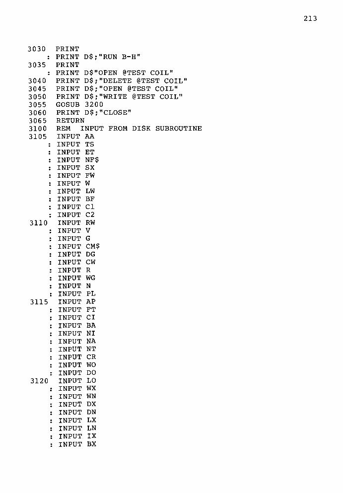
213
3 030 PRINT
: PRINT D$;"RUNB-H"
3035 PRINT
: PRINT D$"OPEN @TESTCOIL"
3040 PRINT D$; "DELETE TESTCOIL"
3045 PRINT D$;"OPEN @TESTCOIL"
3050 PRINT D$;"WRITE @TESTCOIL"
3055 GOSUB 3200
3060 PRINT D$;"CLOSE"
3065 RETURN
3100 REM INPUT FROM DISK SUBROUTINE
3105 INPUT AA
INPUT TS
INPUT ET
INPUT NF$
INPUT SX
INPUT FW
INPUT W
INPUT LW
INPUT BF
INPUT CI
INPUT C2
3110 INPUT RW
INPUT V
INPUT G
INPUT CM$
INPUT DG
INPUT CW
INPUT R
INPUT WG
INPUT N
INPUT PL
3115 INPUT AP
INPUT FT
INPUT CI
INPUT BA
INPUT NI
INPUT NA
INPUT NT
INPUT CR
INPUT WO
INPUT DO
3120 INPUT LO
INPUT WX
INPUT WN
INPUT DX
INPUT DN
INPUT LX
INPUT LN
INPUT IX
INPUT BX
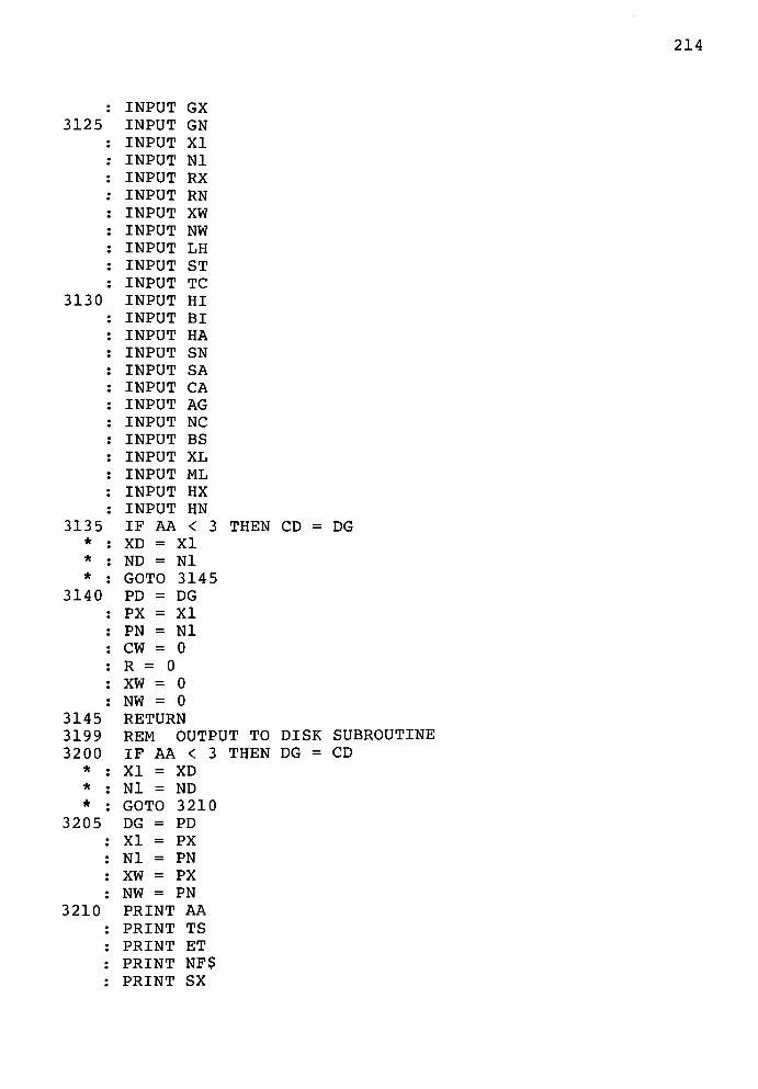
214
3125
3130
3135*
*
*
3140
3145
3199
3200*
*
*
3205
3210
INPUT GX
INPUT GN
INPUT XI
INPUT NI
INPUT RX
INPUT RN
INPUT XW
INPUT NW
INPUT LH
INPUT ST
INPUT TC
INPUT HI
INPUT BI
INPUT HA
INPUT SN
INPUT SA
INPUT CA
INPUT AG
INPUT NC
INPUT BS
INPUT XL
INPUT ML
INPUT HX
INPUT HN
IF AA < 3
XD = XI
ND = NI
GOTO 3145
PD = DG
PX = XI
PN = NI
CW = 0
R = 0
XW = 0
NW = 0
RETURN
REM OUTPUT TO DISK SUBROUTINE
IF AA < 3 THEN DG = CD
XI = XD
NI = ND
GOTO 3210
THEN CD = DG
DG
XI
NI
XW
NW
PD
PX
PN
PX
PN
PRINT AA
PRINT TS
PRINT ET
PRINT NF$
PRINT SX
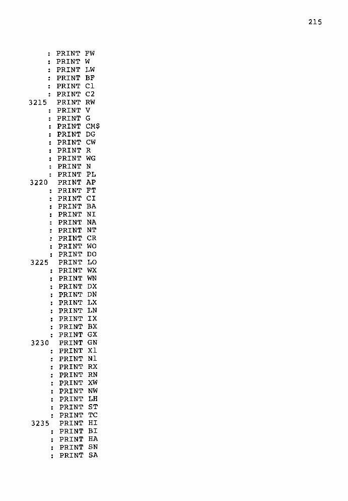
215
3215
3220
3225
3230
3235
PRINT FW
PRINT W
PRINT LW
PRINT BF
PRINT CI
PRINT C2
PRINT RW
PRINT V
PRINT G
PRINT CM$
PRINT DG
PRINT CW
PRINT R
PRINT WG
PRINT N
PRINT PL
PRINT AP
PRINT FT
PRINT CI
PRINT BA
PRINT NI
PRINT NA
PRINT NT
PRINT CR
PRINT WO
PRINT DO
PRINT LO
PRINT WX
PRINT WN
PRINT DX
PRINT DN
PRINT LX
PRINT LN
PRINT IX
PRINT BX
PRINT GX
PRINT GN
PRINT XI
PRINT NI
PRINT RX
PRINT RN
PRINT XW
PRINT NW
PRINT LH
PRINT ST
PRINT TC
PRINT HI
PRINT BI
PRINT HA
PRINT SN
PRINT SA
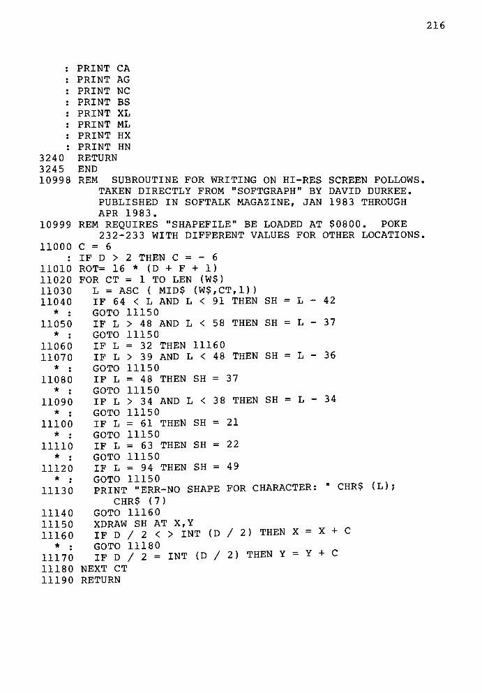
216
3240
3245
10998
10999
11000
11010
11020
11030
11040
* .
11050
*:
11060
11070
*:
11080
*:
11090
*:
11100
*:
11110
*:
11120
*:
11130
11140
11150
11160
*:
11170
11180
11190
PRINT CA
PRINT AG
PRINT NC
PRINT BS
PRINT XL
PRINT ML
PRINT HX
PRINT HN
RETURN
END
REM SUBROUTINE FOR WRITING ON HI-RES SCREEN FOLLOWS.
TAKEN DIRECTLY FROM"SOFTGRAPH"
BY DAVID DURKEE.
PUBLISHED IN SOFTALK MAGAZINE, JAN 1983 THROUGH
APR 1983.
REM REQUIRES"SHAPEFILE"
BE LOADED AT $08 00. POKE
232-233 WITH DIFFERENT VALUES FOR OTHER LOCATIONS,
C = 6
IF D > 2 THEN C = - 6
ROT= 16 * (D + F + 1)
FOR CT = 1 TO LEN (W$)
L = ASC ( MID$ (W$,CT,1))
IF 64 < L AND L < 91 THEN SH = L - 42
GOTO 11150
IF L > 48 AND L < 58 THEN SH = L - 37
GOTO 11150
IF L = 32 THEN 11160
IF L > 39 AND L < 48 THEN SH = L - 36
GOTO 11150
IF L = 48 THEN SH = 37
GOTO 11150
IF L > 34 AND L < 38 THEN SH = L - 34
GOTO 11150
IF L = 61 THEN SH = 21
GOTO 11150
IF L = 63 THEN SH = 22
GOTO 11150
IF L = 94 THEN SH = 49
GOTO 11150
PRINT"ERR-NO SHAPE
CHR$ (7)
GOTO 11160
XDRAW SH AT X,Y
IF D / 2 < > INT (D / 2) THEN X = X + C
GOTO 11180
IF D / 2 = INT (D / 2) THEN Y = Y + C
NEXT CT
RETURN
FOR CHARACTER:"
CHR$ (L)

217
PROGRAM LENGTH IS 17939 ($4613) BYTES
A 1615, 1635, 1660, 1675, 1690, 1700, 1715, 1725, 1740,
1750, 1765, 1775, 1785, 1795, 1805, 1815, 1825, 1835, 1845,
1855, 1880, 1890, 1900, 1915, 1925, 1935, 1950, 1965, 1975,
1985, 2000, 2030, 2040, 2050, 2065, 2550, 2555, 2560, 3005,
3010
A$ 1600, 1605, 1610, 1620, 1625, 1630, 1680, 1685, 1705,
1710, 1730, 1735, 1755, 1760, 1905, 1910, 1940, 1945, 1955,
1960, 1990, 1995, 2055, 2060, 2105, 2110, 2115, 2130, 2145,
2150, 2155, 2160, 2165, 2170, 2175, 2180, 2190, 2205, 2210,
2215, 2220, 2225, 2230, 2235, 2240, 2245, 2250, 2255, 2260,
2275, 2280, 2285, 2290, 2305, 2310, 2315, 2320, 2325, 2330,
2345, 2350, 2365, 2370, 2385, 2550, 2565, 2620, 2625, 2630,
2695, 2770, 2705, 3005
AA 70, 90, 100, 2185, 2265, 2295, 2950, 3105, 3135, 3200,
3210
AG 3130, 3235
AN 2605
AP 3115, 3220
BA 3115, 3220
BB - 2770
BF 1840, 1845, 2155, 2830, 2905, 3105, 3210
BI 3130, 3235
BN 2605
BS 3130, 3235
BX 1645, 1650, 1655, 1660, 2235, 3120, 3225
BX$ 1640, 1645, 1650
C 11000, 11160, 11170
CI 1820, 1825, 2150, 2830, 2905, 3105, 3210
C2 2025, 2030, 2180, 2835, 2860, 2910, 2925, 3105, 3210
CA 3130, 3235
CD 1920, 1925, 2365, 2955, 3135, 3200
CI 3115, 3220
CM$ 2005, 2010, 2015, 2175, 2750, 3110, 3215
CN 2605
CR 3115, 3220
CT 11020, 11030, 11180
CW 1970, 1975, 2370, 2955, 3110, 3140, 3215
D 45, 450, 795, 980, 985, 1035, 1055, 1110, 1115, 1220,
1725, 1740, 1975, 1985, 2000, 2030, 2040, 2050, 2065, 2140,
2180, 11000, 11010, 11160, 11170
D$ 10, 60, 65, 75, 135, 140, 150, 2570, 2595 , 2600 , 2610 ,
2640, 2650, 2655, 2660, 2665, 2680, 2700, 2760, 2765, 2775,
2890, 2965, 3015, 3030, 3035, 3040, 3045, 3050, 3060
DF$ 80, 115, 120, 135, 140, 2590, 2595, 2600, 2650, 2655,
2660, 2665, 2720, 2730
DG 3110, 3135, 3140, 3200, 3205, 3215
DM$ 2015, 2750, 2760, 2765
DN 1705, 1710, 1715, 2210, 2790, 2865, 2930, 3120, 3225
DO 3115, 3220

218
DX
E
ET
3025,F
Fl
F2
FL
FT
FW
G
GF$
GN
GX
H
HA
HI
HN
HX
IX
K
L
11110
LH
LN
LO
LW
LX
M
740,ML
MM
N
NI
NA
NC
ND
NF$
NI
NT
NW
3205,PD
PL
PN
3140,PX
R
3110,
RK
R2(
1695
670,
70,
3105
45,2835
2845
2110
3115
1800
1905
70,1790
1780
670,3130
3130
1625
1605
1770
670,1103
, HI
3125
1755
2890
1830
1745
90,
890,2830
100,1885
3125
3115
3130
1940
130,3115
3115
1990
3230
2035
3110
2055
3205
2045
670,
3140
35,
30,
, 170
675,
115,
, 321
11010
, 284
, 285
, 322
, 180
, 191
80, 1
, 179
, 178
805
, 323
, 323
, 163
, 161
, 177
685,
0, 11
20, 1
, 323
, 176
, 312
, 183
, 175
95, 2
1075,
, 287
105,
, 189
, 313
, 322
, 323
, 194
155,
, 322
, 322
, 199
, 204
, 321
, 206
, 205
675,
, 321
1785,
1615,
0, 2205, 2790, 2845,680, 690, 805
120, 125, 1305, 1350,0
0, 2855, 2860, 2870,0, 2855, 2865, 2870,
0
5, 2275, 3105, 3210
0, 1915, 2170, 3110,30, 155
5, 2250, 2805, 3125,5, 2245, 2805, 3120,
2915, 3120, 3225
1430, 1475, 2590, 2960,
2910, 2920, 2925, 2935
2915, 2920, 2930, 2935
3215
3230
3225
, 1635, 2260, 3130, 3235
, 1615, 2255, 3130, 3235
, 2240, 3120, 3225
690, 805, 810
40, 11050, 11060, 11070, 11080, 11090, 11100,130
, 1765, 2230, 2795, 2830, 2905, 3120, 3225
, 3225
, 2280, 3105, 3210
, 2225, 2795, 2830,
0, 225, 270, 295, 31!
2835, 2860, 2910, 29:
, 2905, 3130, 3235
550, 990, 1205, 2810
, 2290, 3110, 3215
, 3140, 3200, 3205,
2905, 3120, 3225
.5, 495, 605, 685, 690,125
3230
, 1950, 2310, 2815,
485, 2590, 2710, 271
2845, 3135, 3200
5, 2720, 3105, 3210
0
0
5, 2000, 2320, 2825, 2830, 2835, 3125, 3140,
0, 2385, 3140, 3205
5
0, 2065, 2350, 2895, 2900, 2905, 2910, 2915,
2905, 2930, 3140, 3205
1960, 1965, 2190, 2955,0, 2345, 2895, 2900,
680, 690, 805, 1955,
5
1795, 1855, 1890
1635, 1660, 1675, 1690, 1700, 1715, 1725,

219
1740
R3(
1935
R4(
RN
3230
RW
RW$
RX
S
SA
SH
370,
915,1107
SN
ST
SX
TC
TS
2525
TT
V
W
2925
W$
485,
975,1185
1660
1785
1900
2030
WG
WN
WO
WX
X
470,
950,1055
1615
1750
1855
1985
XI
XD
XL
XW
3205
Y
, 1750, 1765, 1775
25, 1805, 1815, 1825, 1835, 1845,, 1950, 1965, 1975, 1985, 2000, 203
20, 1915
1680, 1685, 1690, 2055, 2060, 233
1865
1860
1670
670,3130
290,
375,
920,
0, 110
2870
670,2855
3125
70,
, 2785
125
1895
1810
, 2930
430,
490,
980,
, 1190
, 1675
, 1795
, 1915
, 2040
1850
1730
3115
1720
20,
475,
955,
, 1110
, 1635
, 1765
, 1880
, 2000
3125
1930
2830
1980
, 3230
430,
, 1870, 1875, 1880, 2160, 311
, 1865, 1870
, 1675, 2045, 2325, 2820, 290
690, 805
, 3235
295, 300, 310, 320, 335, 340
535, 540, 545, 585, 590, 595,925, 1145, 1150, 1155, 1160,80, 11090, 11100, 11110, 1112
, 2875, 2935, 3130, 3235
675, 680, 690, 805, 3125, 32
, 2875, 2920, 3105, 3210
, 3230
115, 120, 125, 655, 660, 780,
, 3105, 3210
1880, 1900, 1925,
0, 2040, 2050, 2065
0, 2820, 2900, 3125,
0, 3215
0, 3125, 3230
, 345, 350, 360, 365,
615, 630, 905, 910,
1165, 11040, 11050,
0, 11150
30
785, 800, 2125, 2195,
, 1900
, 1815
, 3105
435,
795, 9
985, 1
, 1195
, 1690
, 1805
, 1925
, 2050
, 1855
, 1735
, 3220
, 1725
25, 30
480, 4
960, 9
, 1115
, 1650
, 1775
, 1890
, 2010
, 3135
, 1935
, 2875
, 1985
, 2165
, 2145
, 3210
440, 4
30, 93
030, 1
, 1200
, 1700
, 1815
, 1935
, 2065
, 2285
, 1740
, 2215
, 35,
85, 49
65, 97
, 1185
, 1660
, 1785
, 1900
, 2030
,3140
, 2305
, 2905
, 2315
, 3110,
, 2835,
45, 450
5, 940,
035, 10
, 1215,
, 1715,
, 1825,
, 1950,
, 11020
, 3110,
, 2220,
, 2800,
430, 43
3215
2845, 2860, 2865, 2910, 2915,
, 455, 460
945, 950,
40, 1045,
1220, 122
1725, 174
1835, 184
1965, 197
, 11030
3215
2800, 2860, 2925, 3120, 3225
, 465, 470, 475, 480,
955, 960, 965, 970,
1055, 1110, 1115,
5, 1615, 1635, 1650,
0, 1750, 1765, 1775,
5, 1855, 1880, 1890,
5, 1985, 2000, 2010.
795,
975,
1190,
1675,
1795,
1915,
2040,
3200,
2815,
3130,
2825,
2835,
5, 440
805,
980,
1195,
1690,
1805,
1925,
2050,
3205,
2865,
3235
2830,
291
, 44
810,
985,
120
170
181
193
206
323
313
286(
0, 3120, 3225
5, 450, 455, 460, 465,
930, 935, 940, 945,
1030, 1035, 1040, 1045,
0, 1215, 1220, 1225,
0, 1715, 1725, 1740,
5, 1825, 1835, 1845,
5, 1950, 1965, 1975,
5, 11150, 11160
0
5, 3200
0, 2925, 3125, 3140,
435, 440, 445, 450, 455, 460, 465, 470, 475, 480,
220
APPENDIX D
B-H PROGRAM MODULE
D.l Program Listing 222
D.2 Program Length and XRef 232
221
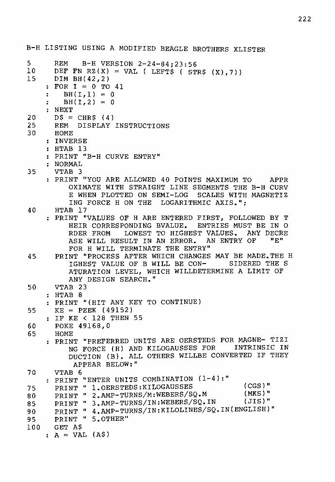
222
B-H LISTING USING A MODIFIED BEAGLE BROTHERS XLISTER
5
10
15
20
25
30
35
40
45
50
55
60
65
70
REM B-H VERSION 2-24-84 ; 23 : 56
DEF FN RZ(X) = VAL ( LEFT$ ( STR$DIM BH(42,2)
FOR I = 0 TO 41
= 0
= 0
(X),7))
BH(I,1)
BH(I,2)
NEXT
D$ = CHR$ (4)REM DISPLAY INSTRUCTIONS
HOME
INVERSE
HTAB 13
PRINT "B-H CURVEENTRY"
NORMAL
VTAB 3
PRINT "YOU ARE ALLOWED 4 0 POINTS MAXIMUM TO APPR
OXIMATE WITH STRAIGHT LINE SEGMENTS THE B-H CURV
E WHEN PLOTTED ON SEMI-LOG SCALES WITH MAGNETIZ
ING FORCE H ON THE LOGARITHMIC AXIS.";
HTAB 17
PRINT "VALUES OF H ARE ENTERED FIRST, FOLLOWED BY T
HEIR CORRESPONDING BVALUE. ENTRIES MUST BE IN O
RDER FROM LOWEST TO HIGHEST VALUES. ANY DECRE
ASE WILL RESULT IN AN ERROR. AN ENTRY OF"E"
FOR H WILL TERMINATE THEENTRY"
PRINT "PROCESS AFTER WHICH CHANGES MAY BE MADE. THE H
IGHEST VALUE OF B WILL BE CON- SIDERED THE S
ATURATION LEVEL, WHICH WILLDETERMINE A LIMIT OF
ANY DESIGNSEARCH."
VTAB 2 3
HTAB 8
PRINT "(HIT ANY KEY TO CONTINUE)
KE = PEEK (49152)
IF KE < 128 THEN 55
POKE 49168,0
HOME
PRINT "PREFERRED UNITS ARE OERSTEDS
NG FORCE (H) AND
DUCTION (B). ALL
APPEARBELOW:"
VTAB 6
ENTER UNITS COMBINATION
1. OERSTEDS:KILOGAUSSES(CGS)"
2.AMP-TURNS/M:WEBERS/SQ.M(MKS)"
3.AMP-TURNS/IN :WEBERS/SQ. IN(JIS)"
4 .AMP-TURNS/IN :KILOLINES/SQ . IN ( ENGLISH )
5.OTHER"
(A$)
: PRINT"
75 PRINT"
80 PRINT"
85 PRINT"
90 PRINT"
95 PRINT"
100 GET A$
: A = VAL
FOR MAGNE- TIZI
KILOGAUSSES FOR INTRINSIC IN
OTHERS WILLBE CONVERTED IF THEY
(1-4)
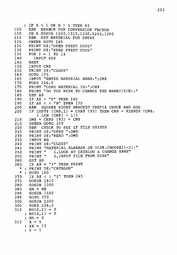
223
: IF A < 1 OR A > 5 THEN 6 5
105 REM BRANCH FOR CONVERSION FACTOR
110 ON A GOSUB 1200,1215,1230,1245,1260
115 REM GET MATERIAL FOR ENTRY
12 0 ONERR GOTO 165
125 PRINT D$;"OPEN @TESTCOIL"
130 PRINT D$;"READ @TESTCOIL"
135 FOR I = 1 TO 14
140 INPUT ZZ$
145 NEXT
150 INPUT CM$
155 PRINT D$;"CLOSE"
160 GOTO 175
165 INPUT "ENTER MATERIAL NAME:";CM$
170 POKE 216,0
175 PRINT "CORE MATERIAL IS:";CM$
18 0 PRINT "DO YOU WISH TO CHANGE THENAME?(Y/N):"
185 GET A$
190 IF A$ ="Y"
THEN 165
195 IF A$ < >"N"
THEN 175
2 00 REM SQUARE RIGHT BRACKET PREFIX CHECK AND ADD
205 IF LEFT$ (CM$,1) = CHR$ (93) THEN CM$ = RIGHT$ (CM$,
( LEN ( CM$ ) - 1 ) )
210 DM$ = CHR$ (93) + CM$
215 ONERR GOTO 300
220 REM CHECK TO SEE IF FILE EXISTS
22 5 PRINT D$;"OPEN ";DM$
230 PRINT D$;"READ ";DM$
23 5 INPUT BB
240 PRINT D$;"CLOSE"
245 PRINT "MATERIAL ALREADY ON DISK. CHOOSE( 1-2 ):"
250 PRINT" l.LOOK AT CATALOG & CHANGE
NAME"
255 PRINT"
2. INPUT FILE FROMDISK"
260 GET A$
265 IF A$ ="1"
THEN PRINT
*: PRINT D$;
"CATALOG"
*: GOTO 165
270 IF A$ < >"2"
THEN 245
275 GOSUB 1610
280 GOSUB 1300
285 EN = NH
290 GOSUB 1500
295 GOTO 370
300 GOSUB 1300
305 POKE 216,0
310 BH(0,2) = 0
: BH(0,1) = 0
: NH = 0
315 X = 5
: XX = 13
: Y = 1
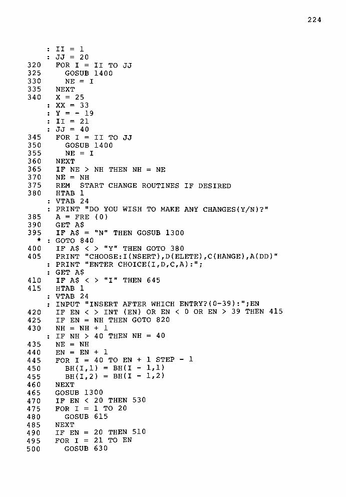
224
: II = 1
: JJ = 2 0
320 FOR I = II TO JJ
325 GOSUB 1400
330 NE = I
335 NEXT
340 X = 25
XX = 33
Y = - 19
II = 21
JJ = 40
345 FOR I = II TO JJ
350 GOSUB 1400
355 NE = I
36 0 NEXT
365 IF NE > NH THEN NH = NE
370 NE = NH
375 REM START CHANGE ROUTINES IF DESIRED
380 HTAB 1
: VTAB 24
: PRINT "DO YOU WISH TO MAKE ANY CHANGES (Y/N )?"
385 A = FRE (0)
390 GET A$
395 IF A$ ="N"
THEN GOSUB 1300*
: GOTO 840
400 IF A$ < >"Y"
THEN GOTO 380
4 05 PRINT "CHOOSE: I (NSERT) ,D(ELETE) ,C(HANGE)
: PRINT "ENTER CHOICE (I,D,C, A) :";: GET A$
410 IF A$ < >"I"
THEN 645
415 HTAB 1
: VTAB 24
: INPUT "INSERT AFTER WHICH ENTRY? ( 0-39):"
;EN
420 IF EN < > INT (EN) OR EN < 0 OR EN > 39 THEN 415
425 IF EN = NH THEN GOTO 820
430 NH = NH + 1
: IF NH > 40 THEN NH = 40
435 NE = NH
440 EN = EN + 1
445 FOR I = 40 TO EN + 1 STEP - 1
450 BH(I,1) = BH(I - 1,1)
455 BH(I,2) = BH(I - 1,2)
460 NEXT
465 GOSUB 1300
470 IF EN < 20 THEN 530
475 FOR I = 1 TO 20
480 GOSUB 615
4 85 NEXT
490 IF EN = 20 THEN 510
495 FOR I = 21 TO EN
500 GOSUB 630
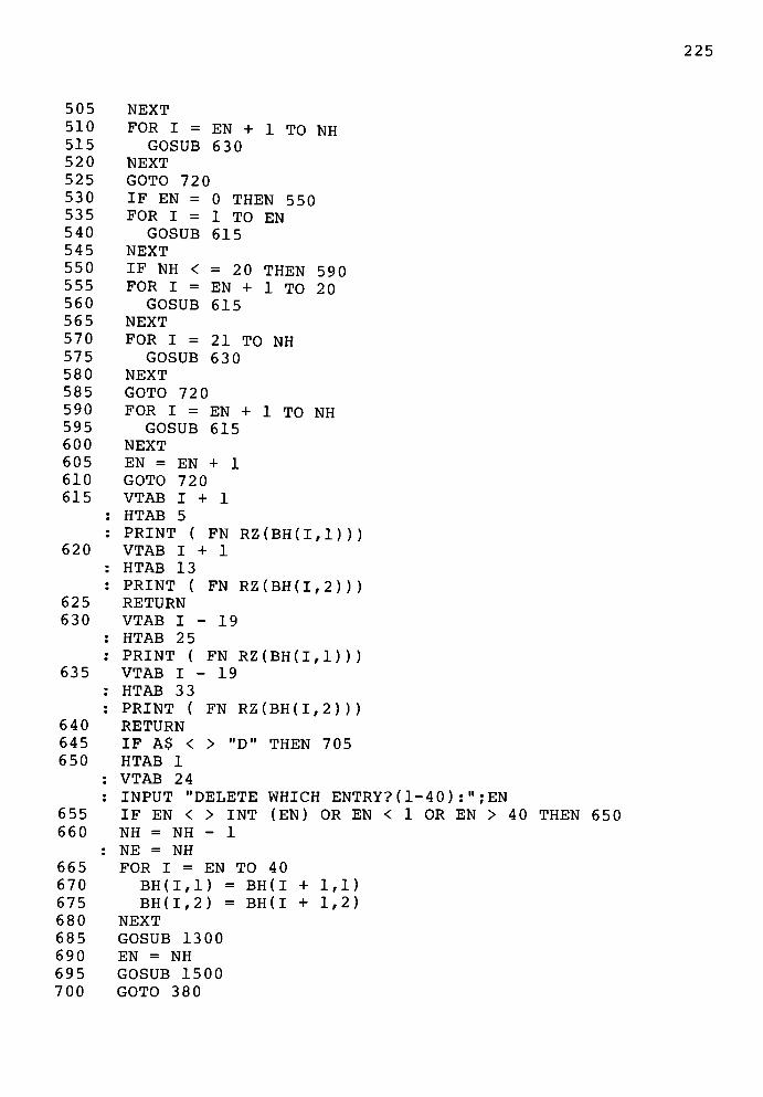
225
505 NEXT
510 FOR I = EN + 1 TO NH
515 GOSUB 630
520 NEXT
525 GOTO 72 0
530 IF EN = 0 THEN 550
535 FOR I = 1 TO EN
540 GOSUB 615
545 NEXT
550 IF NH < = 20 THEN 590
555 FOR I = EN + 1 TO 20
560 GOSUB 615
565 NEXT
570 FOR I = 21 TO NH
575 GOSUB 630
580 NEXT
585 GOTO 72 0
590 FOR I = EN + 1 TO NH
595 GOSUB 615
600 NEXT
605 EN = EN + 1
610 GOTO 72 0
615 VTAB I + 1
: HTAB 5
: PRINT ( FN RZ(BH(I,1) ) )620 VTAB I + 1
: HTAB 13
: PRINT ( FN RZ(BH(I,2)))625 RETURN
630 VTAB 1-19
: HTAB 25
: PRINT ( FN RZ(BH(I,1)))
635 VTAB 1-19
: HTAB 3 3
: PRINT ( FN RZ(BH(I,2)))
640 RETURN
645 IF A$ < >"D"
THEN 705
650 HTAB 1
: VTAB 24
: INPUT "DELETE WHICH ENTRY? ( 1-40 ):"
;EN
655 IF EN < > INT (EN) OR EN < 1 OR EN > 40 THEN 650
660 NH = NH - 1
: NE = NH
665 FOR I = EN TO 4 0
670 BH(I,1) = BH(I + 1,1)
675 BH(I,2) = BH(I + 1,2)
680 NEXT
685 GOSUB 1300
690 EN = NH
695 GOSUB 1500
700 GOTO 380
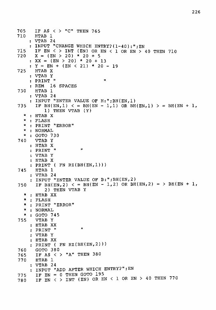
226
705 IF A$ < >"C"
THEN 765
710 HTAB 1
: VTAB 24
: INPUT "CHANGE WHICH ENTRY? ( 1-40):"
;EN
715 IF EN < > INT (EN) OR EN < 1 OR EN > 40 THEN 710
720 X = (EN > 20) * 20 + 5
: XX = (EN > 20) * 20 + 13
: Y = EN + (EN < 21) * 20 - 19
725 HTAB X
: VTAB Y
: PRINT" "
: REM 16 SPACES
730 HTAB 1
: VTAB 24
: INPUT "ENTER VALUE OF H:";BH(EN,1)
735 IF BH(EN,1) < = BH(EN - 1,1) OR BH(EN,1) > = BH(EN + 1,
1) THEN VTAB (Y)*
: HTAB X
*: FLASH
"ERROR"
*: NORMAL
*: GOTO 730
740 VTAB Y
HTAB X
PRINT" "
VTAB Y
HTAB X
PRINT ( FN RZ(BH(EN,1) ) )
745 HTAB 1
: VTAB 24
: INPUT "ENTER VALUE OF B:";BH(EN,2)
750 IF BH(EN,2) < = BH(EN - 1,2) OR BH(EN,2) = > BH(EN + 1,
2 ) THEN VTAB Y
*: HTAB XX
*: FLASH
"ERROR"
*: NORMAL
*: GOTO 745
755 VTAB Y
HTAB XX
PRINT"
VTAB Y
HTAB XX
PRINT ( FN RZ(BH(EN,2) ) )
760 GOTO 380
765 IF A$ < >"A"
THEN 380
77 0 HTAB 1
: VTAB 24
: INPUT "ADD AFTER WHICH ENTRY?"; EN
775
"
IF EN = 0 THEN GOTO 195
780 IF EN < > INT (EN) OR EN < 1 OR EN > 40 THEN 770
227
785
790
795
800
805
810
815
820
*
*
*
825
830
835
840
845
850
855
860
865
870
875
880
885
NH = EN
NE = EN
FOR I = EN + 1 TO 4 0
BH(I,1) = 0
BH(I,2) = 0
NEXT
GOSUB 1300
GOSUB 1500
IF EN > 19 THEN X = 25
XX = 33
Y = - 19
II = EN + 1
JJ = 40
GOTO 345
X = 5
XX = 13
Y = 1
II = EN + 1
JJ = 20
GOTO 32 0
REM BEGIN CONVERSION TO KILOGAUSSES AND OERSTEDS
GOSUB 13 00
INVERSE
VTAB 22
HTAB 5
PRINT "VALUES IN OERSTEDS :KILOGAUSSES"
NORMAL
VTAB 3
HTAB 5
POKE 34,22
II = 1
JJ = 20 + (NH
890
895
900
< 20)
FOR I = II TO JJ
BH(I,1) = BH(I,1)* FH
VTAB I + 1
HTAB 5
PRINT ( FN RZ(BH(I,1) ) )
BH(I,2) = BH(I,2)* FB
VTAB I + 1
HTAB 13
PRINT ( FN RZ(BH(I,2) ) )
NEXT
IF NH < 21 THEN 940
X = 25
XX = 33
Y = - 19
II = 21
JJ = NH
FOR I = II TO JJ
BH(I,1) = BH(I,1)* FH
VTAB (I - 19)
* (NH - 20)
228
: HTAB 25
: PRINT ( FN RZ(BH(I,1)))905 BH(I,2) = BH(I,2) * FB
910 VTAB (I + Y)
: HTAB XX
: PRINT ( FN RZ(BH(I,2)))915 NEXT
92 0 REM CLEAR SCREEN AND SAVE MATERIAL TO DISK
925 POKE 34,0
930 DM$ = CHR$ (93) + CM$
935 ONERR GOTO 1095
940 PRINT
: PRINT D$;"OPEN"
;DM$
945 PRINT D$; "DELETE"
;DM$
950 PRINT D$;"OPEN ";DM$955 PRINT D$; "WRITE ";DM$960 PRINT BH(NH,2)
965 PRINT NH
970 FOR I = 1 TO NH
975 PRINT BH(I,1)
: PRINT BH(I,2)
980 NEXT
985 PRINT D$;"CLOSE"
99 0 REM REPEAT ENTRY PROCESS OR EXIT
995 POKE 34,0
: HOME
1000 PRINT "CHOOSE(1-3):"
1005 PRINT"
1. RETURN TOINPUT/OUTPUT"
1010 PRINT"
2. ENTER ANOTHERMATERIAL"
1015 PRINT"
3.QUIT"
1020 GET A$
: A = VAL (A$)
1025 IF A = 3 THEN END
1030 IF A = 2 THEN GOTO 165
1035 IF A < > 1 THEN GOTO 1000
1040 PRINT
: PRINT D$;"OPEN RUNTYPE"
1045 PRINT D$;"READ RUNTYPE"
1050 INPUT AA
: INPUT TS
: INPUT ET
: INPUT NF$
1055 PRINT D$;"CLOSE"
1060 ET = 3
1065 PRINT D$; "DELETE RUNTYPE"
1070 PRINT D$;"OPEN RUNTYPE"
1075 PRINT D$; "WRITE RUNTYPE"
1080 PRINT AA
: PRINT TS
: PRINT ET
: PRINT NF$
229
1085 PRINT D$;"CLOSE"
1087 HOME
VTAB 12
HTAB 6
INVERSE
PRINT "LOADING INPUT/OUTPUT MODULE"
NORMAL
1090 PRINT
: PRINT D$;"RUN PAGE2-A"
1095 INPUT "ENTER FILENAME"
;CM$
: DM$ = CHR$ (93) + CM$
1100 GOTO 940
1199 REM CONVERSION FACTOR SUBROUTINES
1200 FH = 1
1205 FB = 1
1210 RETURN
1215 FH =.01257
: REM MARKS HANDBOOK, EQUALS 4*PI/1000
1220 FB = 10
1225 RETURN
1230 FH =.49474
: REM .4*(PI)/2.54
1235 FB =.006452
: REM 10*.0254i2
1240 RETURN
1245 FH =.49474
: REM .4(PI)/2.54
1250 FB =
1255 RETURN
1260 INPUT "INPUT RATIO OF 1 OERSTED TO YOUR H UNITS: ";FH
1265 INPUT "INPUT RATIO OF 1 KILOGAUSS TO YOUR B UNITs:";FB
1299 REM HEADER GENERATOR SUBROUTINE
1300 POKE 34,0
1305 HOME
1310 POKE 34,22
1315 INVERSE
: VTAB 1
: HTAB 5
: PRINT"
H"
: VTAB 1
: HTAB 13
: PRINT"
B"
VTAB 1
HTAB 25
PRINT"
H
VTAB 1
HTAB 33
PRINT"
B
NORMAL
1320 FOR I = 1 TO 9
VTAB (I + 1)
230
HTAB 2
PRINTI;")"
NEXT
FOR I = 10 TO 2 0
VTAB (I + 1)HTAB 1
PRINT I ;"
)"
NEXT
FOR I = 21 TO 40
VTAB (I - 19)
HTAB 21
PRINTI;")"
NEXT
1325 INVERSE
VTAB 22
HTAB 5
PRINT "VALUES ARE IN UNITS OFENTRY"
NORMAL
VTAB 3
HTAB 4
POKE 34,22
13 3 0 RETURN
13 9 9 REM READ IN FROM KEYBOARD SUBROUTINE
1400 HTAB 1
: VTAB 24
: INPUT "ENTER VALUE OF H:";H$
1405 IF H$ ="E"
THEN GOTO 365
1410 BH(I,1) = VAL (H$)
1415 IF BH(I,1) < = BH(I - 1,1) THEN VTAB (I + Y)*
: HTAB X
*: FLASH
"ERROR"
*: NORMAL
*: GOTO 1400
1420 VTAB (I + Y)
HTAB X
PRINT"
VTAB (I + Y)
HTAB X
PRINT ( FN RZ(BH(I,1) ) )
1425 VTAB 24
: INPUT "ENTER VALUE OF B:";B$
1430 IF B$ ="E"
THEN GOTO 365
1435 BH(I,2) = VAL (B$)
1440 IF BH(I,2) < = BH(I - 1,2) THEN VTAB (I + Y)
*: HTAB XX
*: FLASH
"ERROR"
*: NORMAL
*: GOTO 1425
1445 VTAB (I + Y)
231
HTAB XX
PRINT" "
VTAB (I + Y)
HTAB XX
PRINT ( FN RZ(BH(I,2) ) )
14 50 RETURN
1500 REM PRINT OUT SUBROUTINE FOR EXISTING VALUES
1505 IF EN < 21 THEN GOTO 1535
1510 X = 25
: XX = 33
: Y = - 19
1515 FOR I = 21 TO EN
152 0 VTAB I + Y
: HTAB X
: PRINT ( FN RZ(BH(I,1) ) )
1525 VTAB I + Y
: HTAB XX
: PRINT ( FN RZ(BH(I,2) ) )
1530 NEXT
1535 X = 5
: XX = 13
: Y = 1
1540 SC = 20
: IF EN < 20 THEN SC = EN
1545 FOR I = 1 TO SC
1550 VTAB I + Y
: HTAB X
: PRINT ( FN RZ(BH(I,1) ))
1555 VTAB I + Y
: HTAB XX
: PRINT ( FN RZ(BH(I,2) ) )
1560 NEXT
1565 RETURN
1600 REM READ IN FROM DISK SUBROUTINE
1605 INPUT "ENTER FILENAME:"
;CM$
1610 DM$ = CHR$ (93) + CM$
1615 ONERR GOTO 1600
1620 PRINT
: PRINT D$;"OPEN ";DM$
1625 PRINT D$;"READ ";DM$
1630 INPUT BS
: INPUT NH
1635 FOR I = 1 TO NH
1640 INPUT BH(I,D
1645 INPUT BH(I,2)
1650 NEXT
1655 PRINT D$;"CLOSE"
1660 POKE 216,0
1665 RETURN

232
PROGRAM LENGTH IS 6938 ($1B1A) BYTES
A 100, 110, 385, 1020, 1025, 1030, 1035
A$ 100, 185, 190, 195, 260, 265, 270, 390, 395, 400, 405,410, 645, 705, 765, 1020
AA 1050, 1080
B$ 1425, 1430, 1435
BB 235
BH( 15, 310, 450, 615, 620, 630, 635, 670, 675, 730,735, 740, 745, 750, 755, 795, 800, 855, 860, 865, 870, 895,900, 905, 910, 960, 975, 1410, 1415, 1420, 1435, 1440, 1445,1520, 1525, 1550, 1555, 1640, 1645
BS 1630
CM$ 150, 165, 175, 205, 210, 930, 1095, 1605, 1610
D$ 20, 125, 130, 155, 225, 230, 240, 265, 940, 945, 950,955, 985, 1040, 1045, 1055, 1065, 1070, 1075, 1085, 1090,1620, 1625, 1655
DM$ 210, 225, 230, 930, 940, 945, 950, 955, 1095, 1610,1620, 1625
E 40
EN 285, 415, 420, 425, 440, 445, 470, 490, 495, 510, 530,
535, 555, 590, 605, 650, 655, 665, 690, 710, 715, 720, 730,735, 740, 745, 750, 755, 770, 775, 780, 785, 790, 820, 825,
1505, 1515, 1540
ET 1050, 1060, 1080
FB 865, 905, 1205, 1220, 1235, 1250, 1265
FH 855, 895, 1200, 1215, 1230, 1245, 1260
H$ 1400, 1405, 1410
I 15, 135, 320, 330, 345, 355, 445, 450, 455, 475, 495,
510, 535, 555, 570, 590, 615, 620, 630, 635, 665, 670, 675,
790, 795, 800, 850, 855, 860, 865, 870, 890, 895, 900, 905,
910, 970, 975, 1320, 1410, 1415, 1420, 1435, 1440, 1445,
1515, 1520, 1525, 1545, 1550, 1555, 1635, 1640, 1645
II 315, 320, 340, 345, 820, 825, 845, 850, 885, 890
JJ 315, 320, 340, 345, 820, 825, 845, 850, 885, 890
KE 55
NE 330, 355, 365, 370, 435, 660, 785
NF$ 1050, 1080
NH 285, 310, 365, 370, 425, 430, 435, 510, 550, 570, 590,
660, 690, 785, 845, 880, 885, 960, 965, 970, 1630, 1635
RZ( 10, 615, 620, 630, 635, 740, 755, 860, 870, 900, 910,
1420, 1445, 1520, 1525, 1550, 1555
SC 1540, 1545
TS 1050, 1080
X 10, 315, 340, 720, 725, 735, 740, 820, 825, 885, 1415,
1420, 1510, 1520, 1535, 1550
XX 315, 340, 720, 750, 755, 820, 825, 885, 910, 1440,
1445, 1510, 1525, 1535, 1555
Y 315, 340, 720, 725, 735, 740, 750, 755, 820, 825, 885,
910, 1415, 1420, 1440, 1445, 1510, 1520, 1525, 1535, 1550, 1555
ZZ$ 140

APPENDIX E
ANALYSIS PROGRAM MODULE
E.l Program Listing 234
E.2 Program Length and XRef 249
234
ANALYSIS LISTING USING A MODIFIED BEAGLE BROTHERS XLISTER
5 REM ANALYSIS PORTION OF
10 DIM BH(41,2)
15 PI = 3 .141592654
20 EP =. 00001
25 SF = 0
: PF = 0
30 Kl = 2 .8696831
35 K2 =. 4 * PI
40 D$ = CHR$ (4)
45 REM READ INPUT DATA
50 PRINT D$;"OPEN @TESTCOIL"
55 PRINT D$;"READ @TESTCOIL"
60 INPUT AA
INPUT TS
INPUT ET
INPUT NF$
INPUT SX
INPUT FW
INPUT W
INPUT LW
INPUT BF
INPUT CI
INPUT C2
65 INPUT RW
INPUT V
INPUT G
INPUT CM$
INPUT DG
: INPUT CW
: INPUT R
: INPUT WG
: INPUT N
: INPUT PL
70 INPUT AP
: INPUT FT
: INPUT CI
: INPUT BA
: INPUT NI
: INPUT NA
: INPUT NT
: INPUT CR
: INPUT WO
: INPUT DO
75 INPUT LO
: INPUT WX
: INPUT WN
: INPUT DX
: INPUT DN
: INPUT LX
235
: INPUT LN
: INPUT IX
: INPUT BX
: INPUT GX
80 INPUT GN
: INPUT XI
: INPUT NI
: INPUT RX
: INPUT RN
: INPUT XW
: INPUT NW
: INPUT LH
: INPUT ST
: INPUT TC
85 INPUT HI
: INPUT BI
INPUT HA
INPUT SN
INPUT SA
INPUT CA
INPUT AG
INPUT NC
INPUT BS
INPUT XL
INPUT ML
INPUT HX
INPUT HN
90 PRINT D$;"CLOSE"
95 REM SET UP EQUATION & CONSTANT MODIFIERS FOR DIFFERENT
CONFIGURATIONS
10 0 IF AA = 1 OR AA = 3 THEN M = 1*
: GOTO 110
105 M = 2
110 TS = 3
115 IF AA < 3 THEN CD = DG
*: GOTO 130
120 CD = DG
: CW = CD
; R = CD / 2
125 REM READ CORE MATERIAL FILE
130 DM$ = CHR$ (93) + CM$
135 PRINT D$;"OPEN ";DM$
140 PRINT D$ ; "READ"
;DM$
145 INPUT BS
; INPUT NH
150 FOR I = 1 TO NH
155 INPUT BH(I,1)
160 INPUT BH(I,2)
165 NEXT
170 PRINT D$;"CLOSE"
175 REM BEGIN ANALYSIS

236
180 AG= (CD-2*R) * (CW-2*R)+2*(CD-2*R)
* (R + G / 2) + 2 * (CW - 2 *R) * (R+G/2) +
PI * (R + G / 2) f 2
: REM AREA OF THE AIRGAP, CORRECTED FOR FRINGING185 PL = 2 * (LW +2*BF+M*FW+M*W+Cl+C2+2
*CW)
: REM STEEL PATH LENGTH
190 AD =.324860745
: BD =.890525717
: REM WIRE CONSTANTS
195 WD = AD * BD i WG
: REM BARE WIRE DIAMETER
200 OI = (8.64333333E - 7 ) / WD / WD
: REM OHMS PER INCH
205 OC = OI / 2.54
: REM OHMS PER CM
210 CP = 2 * (CD + CW + (PI - 4) *R)
: REM CORE PERIMETER
215 WD = WD * 2.54
: REM BARE WIRE DIA IN CM
220 GG = G * 2000
: REM SCALED AIRGAP FOR MU OF 1 WHEN WORKING IN
KILOGAUSS/OERSTED INSTEAD OF GAUSS/OERSTED,MULTIPLIED BY 2 AIRGAPS
225 CA = (CD - 2 *R) * (CW - 2 * R) + 2 * (CD - 2 * R)
*R+2* (CW-2*R) *R+PI*R*R
: REM STEEL CORE AREA
230 REM MUST COMPARE N TO CACULATED VALUE. IF DIFFERENT,ASK IF RW DIFF OR IS BOBBIN OVER/UNDERWOUND .
THEN ALTER CALCULATIONS ACCORDING TO ANSWER.
235 IN =.967
* WG + .221
: REM EFFECTIVE WIRE NUMBER OF INSULATED WIRE
240 ID = (AD * BD f IN) * 2.54
: REM DIA OF INSULATED WIRE
245 W2 = 1 / ID / ID
: REM THEORETICAL WIRES/SQ CM
250 NC = RW * M * LW * FW * W2
: REM CALCULATED THEORETICAL NUMBER OF TURNS
255 IF NC > (N * 1.05) THEN PRINT "BOBBIN IS UNDERFILLED.
CHOOSE ONE:"
"1. EXTRA FLANGE WIDTH FOR
TOLERANCE"
"2. USE A NEW RANDOM WIND
FACTOR"
"3. REVIEW
CALCULATIONS"
*: GOTO 285
260 IF NC < (N *.95)
THEN PRINT "BOBBIN IS OVERFILLED.
CHOOSEONE:"
"
1. CONTINUE WITHOVERFILL"
"2. USE NEW RANDOM WIND
FACTOR"
"3. REVIEW
CALCULATIONS"
*: GOTO 270
26 5 WW = FW
237
270
275
280
285
290
295
300
305
310
315
320
325
330
335
340
345
350
355
360
365
370
375
380
385
390
395
400
*
*
*
*
*
*
GOTO 36 0
GET A$
A = VAL (A$)IF A < 1 OR A > 3 THEN 26 0
WW = FW
ON A GOTO 300,305,315
GET A$
A = VAL (A$)IF A < 1 OR A > 3 THEN GOTO 255
FW
GOTO 300,305,315
WW =
ON A
WW =
GOTO
RW =
IF RW
N / W2 / M / LW / RW
360
RW *
> 1 "RW MUST BE <=1 OR WIRES WON'T
N / NC
THEN PRINTFIT"
GOTO 2 60
GOTO 36 0
PRINT "THEORETICAL NUMBER OF TURNS=";NC
PRINT "SPECIFIED NUMBER OF TURNS=";N
PRINT "THEORETICAL FLANGE FOR SPEC. TURNS=
ID / LW / M
PRINT "THEORETICAL RANDOM WINDFACTOR=l"
PRINT "SPECIFIED RANDOM WIND FACTOR=";RW
PRINT "THEORETICAL SPACE UTILIZATION FACTOR=0. 78 54"
PRINT "CALCULATED SPACE UTILIZATION FACTOR=";N *.7854
* RW / NC
:N ID
GOTO
AP =
: REM
NT =
: REM
CR =
: REM
RA =
: REM
REM
"SPECIFIED SPACE UTILIZATION FACTOR=
255
CP + 2 * PI *
AVERAGE PATH
V / OC / AP
TOTAL AMP TURNS
.7854* RW
(W + WW
LENGTH
/ 2)
OC AP W2
AG /AREA
FIND
OPERATING
FOR I = 1 TO
M * LW * WW * RW
COIL RESISTANCE
CA
RATIO
SEGMENT OF B-H CURVE WHICH STRADDLES THE
POINT
NH
NI = PL * BH(I,1) / K2
NA = BH(I,2)* GG / RA / K2
IF I = 1 AND (NI + NA) > NT
B-H CURVE TOANALYZE"
PRINT "WILL CONTINUE WITH NI ,NA,BI
THEN PRINT "TOO LOW ON
HI = 0
BI = 0
NI = 0
HA = 0
BA = 0
NA = 0

238
*
*
405
410
415
420
425
430
435
440
445
450
455
460
465
470
475
480
485
490
495
500
505
510
515
520
525
530
535
540
545
550
555
560
565
570
575
580
585
GOTO 550
REM VALID FOR SENSITIVITY ANALYSIS ONLY-SHOULD END
IF (NI + NA) > NT THEN GOTO 435
NL = NI
FL = BH(I,2)* CA
NEXT
PRINT "TOO HIGH ON B-H CURVE TOANALYZE"
END
T = - (C / K)
NU
HU
HL
FU
FL
Ml
Al
K5
W
UU
NI
ER
* LOG
NI
BH(I,1)
BH(I - 1,1)
BH(I,2)* CA
BH(I - 1,2) * CA
(FU -
FL) / ( LOG
(70 * K / P)
( HU ) - LOG ( HL ) )
K2 * AG / GG / Ml
Al * NT + LOG (NL) - FL / Ml
- Al * NL + K5 - LOG (NL)
Al * NU - K5 + LOG (NU)
(NL * UU + NU * W) / (W + UU)
- Al * NI + K5 - LOG (NI)
FL THEN GOTO 525
GOTO 505,5,515
IF ABS (ER) < EP *
ON ( SGN (ER) + 2)
NU = NI
GOTO 47 5
NL = NI
GOTO 475
HI = NI * K2 / PL
REM OERSTEDS IN IRON
BI = ((FU - FL)* (HI - HL) / (HU - HL) + FL) / CA
REM KILOGAUSSES IN IRON
BA = BI / RA
REM KILOGAUSSES IN AIR
HA = BA
REM KILO-OERSTEDS IN AIR
NA = HA * GG / K2
REM AMP-TURNS IN AIR
NM = NA + NI
REM TOTAL AMP TURNS
FT = Kl * BA * BA * AG
REM TOTAL FORCE IN OZ
IF SF = 1 THEN RETURN
LH = N * CR * BA * AG / V / 100000
REM INDUCTANCE IN HENRIES
SA = M * LW * (AP + PI * WW)
REM
WO =
REM
DO =
REM
LO =
SURFACE AREA
2 * (CW + M * W
OVERALL WIDTH
2 * (W + FW) + CD
OVERALL DEPTH
2 * (CW + BF) + LW + CI
+ M * FW) + C2
239
590
595
600
605
610
615
620
625
630
635
640
645
650
655
660
665
* (PA +.194)
* (PA +.194)
COEFF,POOR THERMAL CONTACT,
DIFF;ROTERS PP185
REM OVERALL LENGTH
CI = V / CR
REM CURRENT DRAW AT VOLTAGE SPECIFIED
NC = M * LW * FW * W2
SM = SA / 2.54 / 2.54
REM SURF AREA SQ IN
PA = CI * CI * CR / SM
REM WATTS/SQ IN SURF
LK = EXP (PA) / (107.23
+ 191.5)
REM HEAT DISSIPATION
WATTS/SQ IN/DEG TEMP
K = SM * LK
REM HEAT DISSIPATION CAPACITY,WATTS/DEG C
WT = AP * WW * (1.9589E - 02) * LW * 0.7854 * RW
REM WT OF COPPER WIRE, CONSTANTS ARE POUNDS/CC
WIRE PACKING EFFICIENCY AT RW=1
= 180 * WT
REM HEAT CAPACITY OF COPPER IN JOULES/DEG C
P = CI * V
REM COIL POWER
ST = PA / LK
STEADY STATE TEMPERATURE RISE IN DEG C
(((ST < 70) * ST + (ST = > 70) * 70) + 20 + 234)
CR / 254
RESISTANCE @ELEVATED TEMP
V / RE
CURRENT @ELEVATED TEMP
NM
* PI/4
AND
REM
RE =
*
REM
IE =
REM
Tl =
T2
T3
T4
T5
T6
T7
T8
T9
SF
NT
GOSUB
TO
NM
NI
NA
HI
HA
BI
BA
FT
NT
SF
NI
NA
HI
HA
BI
BA
FT
NT
1
NT *
385
FT
Tl
T2
T3
T4
T5
T6
T7
T8
T9
0
CR / RE
240
670 TC = C / K
: REM THERMAL TIME CONSTANT IN SEC. ONE TIME CONSTANT
GETS TEMPERATURE RISE TO 63% OF STEADY STATE.
TWO GIVES 86%. 3 GIVES 95%. 4 GIVES 98%
675 REM OUTPUT ANALYSIS AND COIL PARAMETERS TO DISK
680 IF AA < 3 THEN DG = CD
*: GOTO 690
685 DG = CD
690 PRINT
: PRINT D$; "DELETE @TESTCOIL"
695 PRINT D$;"OPEN @TESTCOIL"
700 PRINT D$; "WRITE @TESTCOIL"
7 05 PRINT AA
PRINT TS
PRINT ET
PRINT NF$
PRINT SX
PRINT FW
PRINT W
PRINT LW
PRINT BF
PRINT CI
PRINT C2
710 PRINT RW
PRINT V
PRINT G
PRINT CM$
PRINT DG
PRINT CW
PRINT R
PRINT WG
PRINT N
PRINT PL
715 PRINT AP
PRINT FT
PRINT CI
PRINT BA
PRINT NI
PRINT NA
PRINT NT
PRINT CR
PRINT WO
PRINT DO
72 0 PRINT LO
PRINT WX
PRINT WN
PRINT DX
PRINT DN
PRINT LX
PRINT LN
PRINT IX
241
PRINT BX
PRINT GX
725 PRINT GN
PRINT XI
: PRINT NI
: PRINT RX
: PRINT RN
: PRINT XW
: PRINT NW
: PRINT LH
: PRINT ST
: PRINT TC
730 PRINT HI
: PRINT BI
: PRINT HA
: PRINT SN
: PRINT SA
: PRINT CA
: PRINT AG
: PRINT NC
: PRINT BS
: PRINT XL
: PRINT ML
: PRINT HX
: PRINT HN
735 PRINT D$;"CLOSE"
740 REM DISPLAY ANALYSIS
745 PRINT "HOW DO YOU WANT ANALYSIS OUTPUT?
750 PRINT"
l.SENT TOPRINTER"
755 PRINT"
2. DISPLAYED ON SCREENONLY"
760 PRINT"
3. NOTDISPLAYED"
765 PRINT "CHOOSE ONE (1-3):"
770 GET A$
A = VAL (A$)
775 IF A == 2 THEN 800
780 IF A == 3 THEN 1355
785 IF A == 1 THEN PRINT
*: INVERSE
*: PRINT "BE SURE PRINTER IS TURNED
ON"
*: NORMAL
*: PRINT "HIT RETURN WHEN
READY"
* . GET A$
790 PRINT
PRINTD$;"PR#1"
PRINT CHR$(9);"80N"
GOTO 800
795 GOTO 745
800 PRINT "COIL NAME:";NF$
805 ON AA GOTO 810,820,815,825

242
810
815
820
825
830
835
840
845
850
855
860
865
870
875
880
885
890
895
900
905
910
915
920
925
930
935
937
*
940
945
950
955
960
965
970
975
980
985
990
995
1000
1005
1010
1015
1020
1025
1030
1035
A$ = "SINGLE BOBBIN, RECTANGULARCORE"
GOTO 830
A$ = "SINGLE BOBBIN, ROUNDCORE"
GOTO 8 30
A$ = "DOUBLE BOBBIN, RECTANGULARCORE"
GOTO 830
A$ = "DOUBLE BOBBIN, ROUNDCORE"
PRINT "COIL TYPE:";A$
PRINT "OPERATING VOLTAGE: ";V
PRINT "COIL RESISTANCE: ";CR
PRINT "CORE MATERIAL: ";CM$
PRINT "THEORETICAL, NO LOSS HOLDING FORCE(OZ ) :";FT
PRINT "EXPECTED HOLDING FORCE (OZ):";(FT *.64)
PRINT "****PHYSICAL DIMENSIONS &CONSTANTS****"
PRINT "OVERALL LENGTH: ";LO
PRINT "OVERALL DEPTH: ";DO
PRINT "OVERALL WIDTH: ";WO
PRINT "FLANGEWIDTH:"
;FW
PRINT "WINDING LENGTH: ";LW
PRINT "BOBBIN WALL THICKNESS:"
;W
PRINT "BOBBIN FLANGE THICKNESS:"
;BF
PRINT "A3RMATURE/BOBBIN CLEARANCE:";Cl
PRINT "WINDING CLEARANCE:";C2
PRINT "AIRGAP :";G
PRINT "STEEL PATH LENGTH: ";PL
IF AA < 3 THEN 935
PRINT "CORE RADIUS: ";R
GOTO 950
PRINT "CORE WIDTH: ";CW
IF A = 2 THEN PRINT "HIT ANY KEY TOCONTINUE"
GET A$
'CORE DEPTH: ";DG
CORNER RADIUS :"
; R
"CORE PERIMETER :
"
; CP
'CORE AREA:";CA
'AIRGAP AREA ( FRINGING ) :"
; AG
WINDING SURFACE AREA:";SA
it ************ * *WINDINGDATA*
*************"
"WIRE GAGE NUMBER: #";WG
'TURNS SPECIFIED: ";N
'TURNS POSSIBLE:";NC
'RANDOM WIND :"
; RW
'WINDING WIDTH: ";WW
'BARE WIRE DIA:";WD
OHMS/CM OF WIRE:";OC
EFFECTIVE INSUL.WG :"
; IN
'INSULATED WIRE DIA:"; ID
'THEORETICAL TURNS/SQCM="
;W2
CURRENT AT";V;"
VOLTS: ";CI
"AVERAGE TURN LENGTH: ";AP
INDUCTANCE ,HENRIES :
"
; LH

243
1037 IF A =
* . GET A$
1040 PRINT
1045 IF ST
1050 PRINT
1055 T = -
1060 PRINT
1065 PRINT
1070 IF ST
* . GOTO 1
1075 PRINT
1080 PRINT
1085 PRINT
1090 PRINT
1095 PRINT
1100 PRINT
1105 PRINT
1110 PRINT
1115 PRINT
1120 PRINT
1125 PRINT
1130 PRINT
1135 PRINT
1137 IF A =
*: GET A$
1140 PRINT
1145 IF LX
*: GOTO 1
1150 PRINT
1155 IF LO
1160 PRINT
1165 IF LO
1170 PRINT
1175 IF DO
1180 PRINT
1185 IF DO
1190 PRINT
1195 IF WO
1200 PRINT
1205 IF WO
1210 IF AA
* . IF DG
*: IF DG
*: GOTO 1
1215 PRINT
1220 IF CW
2 THEN PRINT "HIT ANY KEY TOCONTINUE"
"S.S.TEMP RISE, DEG C:";ST
< = 70 THEN 1065
"****WARNING:COIL EXCEEDS 7 0 DEG CRISE"
"OVERHEATING WILL DEGRADEINSULATION"
(C / K) * ( LOG (P / K - 70) - LOG (P / K))
"TIME TO REACH 7 0 DEGC="
;T;"SEC"
"DO NOT EXCEED THISTIME."
"ALLOW AT LEAST THIS MUCH TIMEBETWEEN"
"ACTUATIONS WHICH ARE OF THISLENGTH"
"THERMAL TIME CONST: ";TC
< = 70 THEN PRINT "RESISTANCE @S. S.TEMP :";RE
080
"RESISTANCE @7 0 DEG C:";RE
"CURRENT @THAT TEMP:";IE
"IDEAL FORCE @THAT TEMP@"
;V;"VOLTS="
;T0
************** *MAGNETIC DATA* ************"
"TOTAL AMP-TURNS ( ACTUAL ) :
"
;NT
"TOTAL AMP-TURNS(AIR+IRON) :";NM
"AMP-TURNS IN IRON:";NI
"AMP-TURNS IN AIR:";NA
"OERSTEDS IN IRON:";HI
"OERSTEDS IN AIR:"; (HA* 1000)
"KILOGAUSSES IN IRON:";BI
"KILOGAUSSES IN AIR:";BA
"IRON SAT KILOGAUSS:";BS
2 THEN PRINT "HIT ANY KEY TOCONTINUE"
********** * *DESIGN CONSTRAINTS***********"
= 0 THEN PRINT"NONE"
350
"MAX OVERALL LENGTH: ";LX
> LX * 1.01 THEN PRINT "***LXVIOLATED"
"MIN OVERALLLENGTH:"
;LN
< LN *.99 THEN PRINT "***LN
VIOLATED"
"MAX OVERALL DEPTH: ";DX
> DX * 1.01 THEN PRINT "***DXVIOLATED"
"MIN OVERALL DEPTH: ";DN
< DN *.99 THEN PRINT "***DN
VIOLATED"
"MAX OVERALL WIDTH: ";WX
> WX * 1.01 THEN PRINT "***WXVIOLATED"
"MIN OVERALL WIDTH: ";WN
< WN *.99 THEN PRINT "***WN
VIOLATED"
= 2 OR AA = 4 THEN PRINT "MAX CORE DIA:";PX
> PX * 1.01 THEN GOSUB 1325
"MIN CORE DIA:";PN
< PN *.99
THEN GOSUB 1330
275
"MAX CORE WIDTH: ";XW
> XW * 1.01 THEN PRINT "***XWVIOLATED"

244
1225
1230
1235
1240
1245
1250
1255
1260
1265
1270
1275
1280
1285
1290
1295
1300
1305
1310
1315
1320
1325
1330
1335*
1337
1340
1345
1350
1355
1360
1365
1370
1375
1380
1385
1390
1395
PRINT "MIN CORE WIDTH: ";NW
IF CW < NW *.99 THEN PRINT "***NW VIOLATED"
PRINT "MAX CORE DEPTH: ";X1
IF DG > XI * 1.01 THEN PRINT "***X1 VIOLATED"
PRINT "MIN CORE DEPTH: ";N1
IF DG < NI *.99 THEN PRINT "***Nl VIOLATED"
PRINT "MAX CORE CORNER RAD:";RX
IF R > RX * 1.01 THEN PRINT "***RX VIOLATED"
PRINT "MIN CORE CORNER RAD:";RN
IF R < RN *.99 THEN PRINT "***RN VIOLATED"
PRINT "MAX CURRENT @";V;"
VOLTS :"; IX
IF CI > IX * 1.01 THEN PRINT "***IX VIOLATED"
PRINT "MAX WIRE GAGE NUMBER:";GX
IF WG > GX * 1.01 THEN PRINT "***GX VIOLATED"
PRINT "MIN WIRE GAGE NUMBER: ";GN
IF WG < GN *.99 THEN PRINT "***GN
VIOLATED"
IF BX = 0 THEN BX = BH(NH,2)
PRINT "MAX KILOGAUSS IN CORE:";BX
IF BI > BX * 1.01 THEN PRINT "***BXVIOLATED"
GOTO 1335
PRINT "***PXVIOLATED"
RETURN
PRINT "***PNVIOLATED"
RETURN
IF A = 2 THEN PRINT "HIT ANY KEY TOCONTINUE"
GET A$
PRINT "DESIGNHINTS:"
PRINT "IF ANY FINAL DIMENSIONS ARE AT ORNEAR"
PRINT "THEIR LIMITS, THEN CHANGING THOSELIMITS"
PRINT "MAY CHANGE THE FINALSOLUTION."
"TEMPERATURE RISE CAN BE REDUCEDBY"
"INCREASING THE SURFACE AREA (ORLX)"
REM RETURN TO PAGE 2-A
PRINTD$;"PR#0"
PRINT D$;"OPEN RUNTYPE"
PRINT D$;"READ RUNTYPE"
INPUT AA
INPUT TS
INPUT ET
INPUT NF$
PRINT D$;"CLOSE"
TS = 4
PRINT D$; "DELETE RUNTYPE"
PRINT D$;"OPEN RUNTYPE"
PRINT D$; "WRITE RUNTYPE"
PRINT AA
PRINT TS
PRINT ET
PRINT NF$
245
1400 PRINT D$;"CLOSE"
1405 PRINTD$;"PR#0"
1410 GOSUB 1500
1415 PRINT
: PRINTD$;"PR#0"
1420 HOME
INVERSE
HTAB 6
VTAB 12
PRINT "LOADING INPUT/OUTPUTMODULE"
NORMAL
VTAB 21
HTAB 5
PRINT "THIS MAY SEEM TO TAKEAWHILE:"
VTAB 23
HTAB 2
PRINT "BUT IT SURE BEATS DOING IT BYHAND!"
PRINT D$;"RUN PAGE2-A"
REM PERFORM VOLTAGE/GAP SENSITIVITY
PRINT "DO YOU WISH TO PERFORM VOLTAGE ANDAIR"
PRINT "GAP SENSITIVITY?(Y/N)"
GET A$
IF A$ ="N"
THEN RETURN
IF A$ < >"Y"
THEN 1500
SF = 1
PRINT "OUTPUT SHOULD BE SENTTO:"
PRINT"
1. SCREENONLY"
PRINT"
2.PRINTER"
GET A$
IF A$ =
IF A$ <
PF = 1
INPUT "ENTER MAX VOLTAGE: ";VX
INPUT "MIN AIRGAP: ";NG
INPUT "MAX AIRGAP: ";XG
INPUT "ENTER NUMBER OF TEST GAPS:";GS
IF GS = 1 THEN SG = 0
GOTO 1585
SG = (XG - NG) / (GS - 1)
VS = INT (VX / .5)+ 1
DIM SS(VS,GS)
HOME
INVERSE
VTAB 12
HTAB 14
PRINT "I'MTHINKING"
NORMAL
1600 G = NG
16 05 REM LOOP FOR GAP TRIALS
1610 FOR II = 1 TO GS
1425
1499
1500
1505
1510
1515
1520
1525
1530
1535
1540
1545
1550
1555
1560
1565
1570
1575
*
1580
1585
1590
1595
"1"THEN 1555
>"2"
THEN 1520
246
1615
1620
1625
1630
1635
1640
1645
1650
1655
1660
1665
1670
1675
1680
1685
1690
1695
1700
1705
1710
1715
1720
1725
1730
1735
1740
1745
1750
1755
1760
1765
1770
1775
1780
1785
1790
1795
1800
1805
1810
1815
1820
1825
1830
GG = G * 2000
V = 0
REM LOOP FOR VOLTAGE STEPS
FOR JJ = 1 TO VS
REM SET V STEP CONSTANT TO A SMALLER VALUE FOR
A SMOOTHER PLOT
V = V + .5
GOSUB 36 0
SS(JJ,II) = FT
NEXT JJ
G = G + SG
NEXT
REM BEGIN SCALE AND PLOT ROUTINE
XI = INT (116 / (VX + 1) )
YI = 166 / ( INT (SS(VS,1) + 5))
HGR
HCOLOR= 3
SCALE= 1
ROT= 0
D = 1
F = 2
POKE - 16302,0
HPLOT 40,0 TO 40,166 TO 272,166
FOR I = 2 TO VS STEP 2
X = XI * I + 40
HPLOT X,163 TO X,169
XL = X - XI
HPLOT XL, 165 TO XL, 167
W$ = STR$ (1/2)
Y = 174
GOSUB 11000
NEXT
FOR I = 4 TO INT (SS(VS,1) + 4) STEP 4
Y = 166 - I * YI
HPLOT 37, Y TO 43, Y
W$ = STR$ (I)
X = 37 - LEN (W$) * 6
Y = Y - 2
GOSUB 11000
NEXT
FOR I = 1 TO GS
X = 40 + XI
Y = 166 - (YI * SS(1,D )
HPLOT X,Y
FOR J = 2 TO VS
X = 40 + XI * J
Y = 166 - (YI * SS(J,D )
HPLOT TO X,Y
NEXT
NEXT
W$ =
"VOLTAGE"
247
1835
1840
1845
1850
*
*
*
*
*
*
*
*
*
*:
*
*:
1855
1860
1865
1870
1875
1880
1885
1890
+ STR$ (NG)
+ STR$ (XG)
0
X = 132
Y = 186
GOSUB 11000
W$ = "IDEAL FORCE"
X = 3
Y = 119
D = 4
GOSUB 11000
D = 1
W$ = "MIN GAP="
X = 50
Y = 12
GOSUB 11000
W$ = "MAX GAP="
X = 180
Y = 157
GOSUB 11000
IF PF = 0 THEN SF =
X = 200
Y = 180
W$ = "HIT ANYKEY"
GOSUB 11000
Y = 187
X = 200
W$ = "TOCONTINUE"
GOSUB 11000
GET A$
TEXT
HOME
RETURN
REM PRINTOUT VALUES FOR SENSITIVITY GRAPH
TEXT
HOME
INVERSE
PRINT "BE SURE PRINTER IS TURNEDON"
NORMAL
PRINT "HIT RETURN WHENREADY"
GET A$
PRINTD$;"PR#1"
CHR$ (9)D$;"PR#1"
CHR$ (9)
FOR I
'G"
"8ON"
"VOLTAGE AND AIRGAP SENSITIVITY FOR ";NF$
"GAP", "VOLTAGE", "IDEAL FORCE (OZ)"
= 1 TO GS
248
1895
1900
1905
1910
1915
10998
10999
11000
11010
11020
11030
11040
* .
11050
*:
11060
11070*
:
11080
*:
11090
*:
11100
* .
11110
*:
11120
*:
11130
11140
11150
11160
*:
11170
11180
11190
FOR J = 1 TO VS
PRINT (NG + (I - 1) * SG),(J *.5),SS(J,I)
NEXT
NEXT
PF = 0
SF = 0
RETURN
REM SUBROUTINE FOR WRITING ON HI-RES SCREEN. TAKEN
DIRECTLY FROM"SOFTGRAPH"
BY DAVID DURKEE.
PUBLISHED IN SOFTALK MAGAZINE, JAN 1983 THROUGH APR
1983
REM REQUIRES"SHAPEFILE"
BE LOADED AT $0800. CHANGE
LOCATIONS 232-233 WITH POKES FOR OTHER SHAPETABLE
START LOCATIONS
C = 6
IF D > 2 THEN C = - 6
ROT= 16 * (D + F + 1)
FOR CT = 1 TO LEN (W$)
L = ASC ( MID$ (W$,CT,1))
IF 64 < L AND L < 91 THEN SH = L - 42
GOTO 11150
IF L > 48 AND L < 58 THEN SH = L - 37
GOTO 11150
IF L = 32 THEN 11160
IF L > 39 AND L < 48 THEN SH = L - 36
GOTO 11150
IF L = 48 THEN SH = 37
GOTO 11150
IF L > 34 AND L < 38 THEN SH = L - 34
GOTO 11150
IF L = 61 THEN SH = 21
GOTO 11150
IF L = 63 THEN SH = 22
GOTO 11150
IF L = 94 THEN SH = 49
GOTO 11150
PRINT "ERR-NO SHAPE FOR CHARACTER:"
CHR$ (L);
CHR$ (7)
GOTO 11160
XDRAW SH AT X,Y
IF D / 2 < > INT (D
GOTO 11180
IF D / 2 = INT (D /
NEXT CT
RETURN
/ 2) THEN X = X + C
2) THEN Y = Y + C

249
PROGRAM LENGTH IS 12606 ($313E) BYTES
A 270, 280, 285, 295, 770, 775, 780, 785A$ 270, 285, 770, 785, 810, 815, 820, 825, 830, 1500, 1505,1510, 1535, 1540, 1545, 1850, 1860Al 465, 470, 475, 480, 490
AA 60, 100, 115, 680, 705, 805, 920, 1210, 1365, 1395AD 190, 195, 240
AG 85, 180, 375, 465, 555, 565, 730, 960AP 70, 360, 365, 370, 570, 620, 715, 1030BA 70, 535, 540, 555, 565, 650, 665, 715, 1130BD 190, 195, 240
BF 60, 185, 585, 705, 895
BH( 10, 155, 160, 390, 395, 415, 440, 445, 450, 455, 1305BI 85, 530, 535, 650, 665, 730, 1125, 1315BS 85, 145, 730, 1135
BX 75, 720, 1305, 1310, 1315
C 430, 625, 670, 1055, 11000, 11160, 11170
CI 60, 185, 585, 705, 900
C2 60, 185, 575, 705, 905
CA 85, 225, 375, 415, 450, 455, 530, 730, 955
CD 115, 120, 180, 210, 225, 580, 680, 685
CI 70, 590, 605, 630, 715, 1025, 1280
CM$ 65, 130, 710, 845
CP 210, 360, 950
CR 70, 370, 565, 590, 605, 640, 655, 715, 840
CT 11020, 11030, 11180
CW 65, 120, 180, 185, 210, 225, 575, 585, 710, 935, 1220,1230
D 1685, 1835, 11000, 11010, 11160, 11170
D$ 40, 50, 55, 90, 135, 140, 170, 690, 695, 700, 735, 790,
1350, 1355, 1360, 1370, 1380, 1385, 1390, 1400, 1405, 1415,
1425, 1865, 1870
DG 65, 115, 120, 680, 685, 710, 940, 1210, 1240, 1250
DM$ 130, 135, 140
DN 75, 720, 1180, 1185
DO 70, 580, 715, 870, 1175, 1185
DX 75, 720, 1170, 1175
E 200, 620
EP 20, 495
ER 490, 495, 500
ET 60, 705, 1365, 1395
F 1685, 11010
FL 415, 455, 460, 470, 495, 530
FT 70, 555, 650, 660, 665, 715, 850, 855, 1650
FU 450, 460, 530
FW 60, 185, 250, 265, 275, 290, 575, 580, 595, 705, 880
G 65, 180, 220, 710, 910, 1600, 1615, 1660
GG 220, 395, 465, 545, 1615
GN 80, 725, 1295, 1300
GS 1570, 1575, 1580, 1590, 1610, 1780, 1890

250
GX
HA
HI
HL
HN
HU
HX
I
455,1890
ID
IE
II
IN
IX
J
JJ
K
Kl
K2
K5
L
1111
LH
LK
LN
LO
LW
LX
M
Ml
ML
N
NI
NA
NC
NF$
NG
NH
NI
550,
NL
NM
NT
NU
NW
OC
OI
P
PA
PF
75, 720
85, 540
85, 525
445,
85,
440,
85,
150.
1700,1900
240,
645,
1610,
235,
, 1285, 1290
, 545, 650, 665
, 530, 650, 665
0, 53046
730
460, 530
730
15
17
5, 160, 385, 39
05, 1725, 1745,
, 730, 1120
, 730, 1115
0, 395, 400, 415, 440, 445, 450,
1750, 1760, 1780, 1790, 1810,
24
10
1
24
0,
75, 720
1800, 1
1630, 1
430, 61
30, 555
35, 390
470, 47
11030,
11120,
80, 565
610, 61
75, 720
75, 585
60, 185
75, 720
100, 10
460,
85,
5, 325, 1015
80
650
0, 1010
, 1275, 1280
805, 1810, 1895, 1900
650, 1655
5, 670, 1055
, 395, 465, 525
5, 480, 490
11040, 11050, 1
11130
, 725, 1035
5, 635
, 1160, 1165
, 720, 865, 115
, 250, 300, 325
, 1145, 1150, 1
, 545
1060, 11070, 11080, 11090, 11100,
65,
80,
70,
85,
60,
46
730
255
725
395
250
705
5,
5,
185,470
5, 1165
, 370, 570, 585, 595, 705, 885
155
250, 300, 325, 370, 570, 575, 595
1560, 1
145, 15
70,
650,
410,
550,
70,
435,
80,
205,
200,
430,
605,
25,
390
665
47
65
365
48
725
36
20
63
61
155
, 26
, 12
, 40
, 25
, 80
580,
0, 3
, 40
,71
0, 4
0, 6
, 40
0, 4
, 12
5, 3
5
0, 1
0, 6
0, 1
0, 300
45, 12
0, 405
5, 260
0, 136
1600,
85, 13
0, 405
5,
75
65
0,85
25
70
110
. 48
11
405
. 50
. 12
. 10
, 305
50
, 545
, 305
5, 13
1840
05
, 410
5
5, 51
00
,470
5
30
05
, 320, 325, 345, 710, 980
, 550, 650, 665, 715, 1110
, 315, 345, 565, 595, 730, 985
95, 1875
, 1900
, 435, 485, 490, 505, 515, 525,
5
, 650, 655, 665, 715, 1095
055
35
850, 1915

251
PI
PL
PN
PX
R
RA
RE
RN
RW
RX
SA
SF
SG
SH
11150
SM
SN
SS(
ST
SX
T
TO
Tl
T2
T3
T4
T5
T6
T7
T8
T9
TC
TS
UU
V
1620,VS
W
VX
W
W$
W2
WD
WG
WN
WO
WT
WW
WX
X
1835,
15, 35, 180, 210, 225, 360, 570, 62065, 185, 390, 525, 710, 9151210
1210
65, 120, 180, 210, 225, 710, 925, 945, 1260, 1270375, 395, 535
640, 645, 655, 1070, 1075
80, 725, 1265, 1270
65, 250, 300, 305, 335, 345, 350, 370, 620, 710, 99080, 725, 1255, 1260
85, 570, 600, 730, 965
25, 560, 650, 665, 1515, 1850, 1915
1575, 1580, 1660, 1900
11040, 11050, 11070, 11080, 11090, 11100, 11110, 11120,
600, 605,
85, 730
615
85, 730
1590, 1650, 1680, 1745, 1790, 1810, 1900
80, 635, 640, 725, 1040, 1045, 1070
60, 70560, 705
430, 1055, 1060
650,
650,
650,
650,
650,
650,
650,
650,
650,
650,
80,
665
665
665
665
665
665
665
665
665
665
670, 725,
705,
1065
1365, 1375, 1395
565, 590, 630, 645, 710, 835, 1025, 1085, 1275,
60, 110,
480, 485
65, 365,1640
1585, 1590, 1630, 1680,
475, 485
1585, 1675
360, 575, 580, 705, 890
1830, 1835,
475,
1555,
60, 185,
1725, 1760,
1700, 1745, 1800, 1895
245,
195,
250,
200,
300,
215,
370,1000
595
195, 200, 215, 1000
65, 195, 235, 710, 975,
75, 720, 1200, 1205
70, 575, 715, 875, 1195,
620, 625
290, 300, 360. nr. l l oc
625
275,
1840,
, 1020
1290,
1205
370,
1845, 1850, 11020, 11030
620,
265, 275, 290, 300, 360, 370,
75, 720, 1190, 1195
1705, 1710, 1715, 1760, 1785,
1840, 1845, 1850, 11150, 111660
1300
570,
1795,
620, 995
1805, 1815, 1830,
XI 80, 725, 1235, 1240XG 1565, 1580, 1845XI 1675, 1705, 1715, 1785, 1805XL 85, 730, 1715, 1720XW 80, 725, 1215, 1220
1835, llll: llll: illl: llllClllio"9*- 181- 1815' 183-
YI 1680, 1750, 1790, 1810
APPENDIX F
COIL DESIGN PROGRAM MODULE
F.l Program Listing 254
F.2 Program Length and XRef 282
253
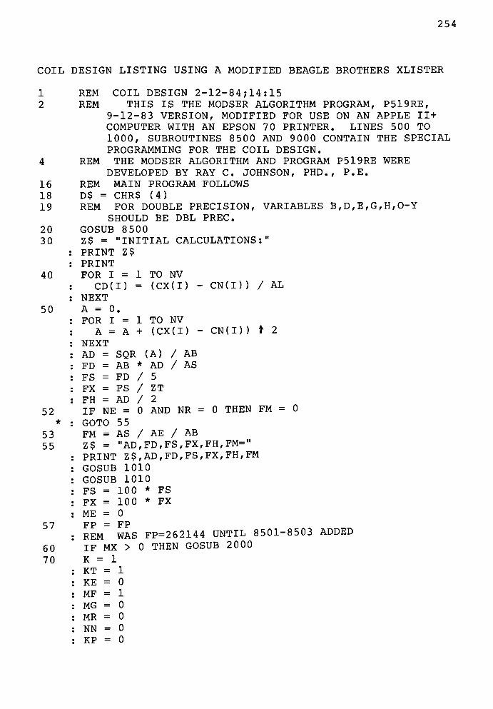
254
COIL DESIGN LISTING USING A MODIFIED BEAGLE BROTHERS XLISTER
1
2
16
18
19
20
30
40
50
52
i
53
55
57
60
70
REM COIL DESIGN 2-12-84 ; 14 : 15
REM THIS IS THE MODSER ALGORITHM PROGRAM, P519RE,
9-12-83 VERSION, MODIFIED FOR USE ON AN APPLE 11+
COMPUTER WITH AN EPSON 70 PRINTER. LINES 500 TO
1000, SUBROUTINES 8500 AND 9 000 CONTAIN THE SPECIAL
PROGRAMMING FOR THE COIL DESIGN.
REM THE MODSER ALGORITHM AND PROGRAM P519RE WERE
DEVELOPED BY RAY C. JOHNSON, PHD., P.E.
REM MAIN PROGRAM FOLLOWS
D$ = CHR$ (4)
REM FOR DOUBLE PRECISION, VARIABLES B,D,E,G, H,0-Y
SHOULD BE DBL PREC.
GOSUB 8500
Z$ = "INITIALCALCULATIONS:"
PRINT Z$
FOR I =
CD(I)
NEXT
A = 0.
FOR I =
A = A
NEXT
AD = SQR (A) / AB
FD = AB * AD / AS
FS = FD / 5
FX = FS / ZT
FH = AD / 2
IF NE = 0 AND NR = 0 THEN FM = 0
GOTO 55
FM = AS / AE / AB
Z$ =
"AD,FD,FS,FX,FH,FM="
PRINT Z$,AD,FD,FS,FX,FH,FM
GOSUB 1010
GOSUB 1010
TO NV
(CX(I)
TO NV
(CX(I)
- CN(I) ) / AL
- CN ( I ) ) t 2
FS =
FX =
ME =
100
100
0
FS
FX
FP = FP
REM WAS FP=262144 UNTIL 8501-8503 ADDED
IF MX > 0 THEN GOSUB 20 00
K = 1
KT
KE
MF
MG
MR
NN
KP
1
0
1
0
0
0
0
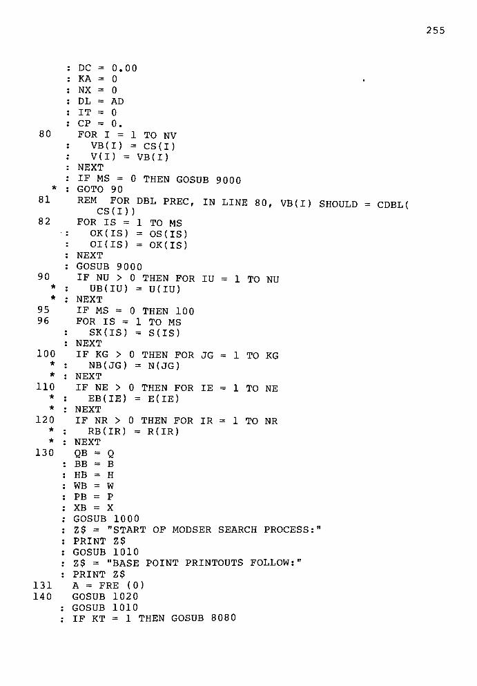
255
80
81
82
90
*
*
95
96
100*
*
110
*
*
120*
*
130
131
140
DC =
KA =
NX =
DL =
IT =
CP =
FOR
: 0.00
= 0
0
: AD
0
: 0.
1 = 1 TO NV
CS(I)
IN LINE 80, VB(I) SHOULD = CDBL(
IU = 1 TO NU
VB(I)
V(I) = VB(I)NEXT
IF MS = 0 THEN GOSUB 9 000
GOTO 90
REM FOR DBL PREC,CS(I))
FOR IS = 1 TO MS
OK (IS) = OS (IS)
OI(IS) = OK(IS)
NEXT
GOSUB 9 0 00
IF NU > 0 THEN FOR
UB(IU) = U(IU)
NEXT
IF MS = 0 THEN 100
FOR IS = 1 TO MS
SK(IS) = S(IS)
NEXT
IF KG > 0 THEN FOR JG
NB(JG) = N(JG)
NEXT
IF NE > 0 THEN FOR
EB(IE) = E(IE)
NEXT
IF NR > 0 THEN FOR
RB(IR) = R(IR)
NEXT
QB = Q
BB = B
HB = H
WB = W
PB = P
XB = X
GOSUB 1000
Z$ = "START OF MODSER SEARCH PROCESS:
PRINT Z$
GOSUB 1010
Z$ = "BASE POINT PRINTOUTSFOLLOW:"
PRINT Z$
A = FRE (0)
GOSUB 102 0
GOSUB 1010
IF KT = 1 THEN GOSUB 8 08 0
1 TO KG
IE = 1 TO NE
IR = 1 TO NR
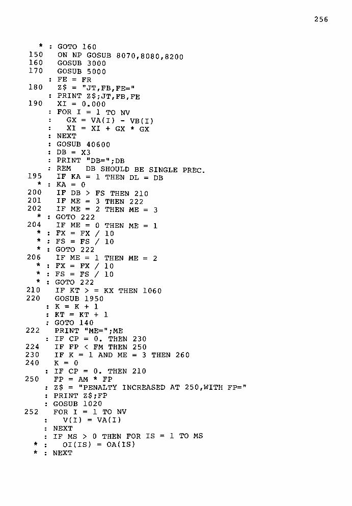
256
*
150
160
170
180
190
195*
200
201
202
*
204
*
*
*
206*
*
*
210
220
222
224
230
240
250
252
*
*
GOTO 16 0
ON NP GOSUB 8070,8080,8200GOSUB 3 000
GOSUB 5000
FE = FR
Z$ = "JT,FB,FE="
PRINT Z$;JT,FB,FE
XI = 0.000
FOR I = 1 TO NV
GX = VA(I) -
VB(I)XI = XI + GX * GX
NEXT
GOSUB 40600
DB = X3
PRINT "DB=";DB
REM DB SHOULD BE SINGLE PREC.IF KA = 1 THEN DL = DB
KA = 0
IF DB >
IF ME =
IF ME = 2 THEN ME = 3
GOTO 222
IF ME = 0 THEN ME = 1
10
FS THEN 210
3
2
THEN 222
THEN ME
10
THEN ME = 2
FX = FX /FS = FS /GOTO 222
IF ME = 1
FX = FX / 10
FS = FS / 10
GOTO 222
IF KT > = KX THEN 1060
GOSUB 1950
K = K + 1
KT = KT + 1
GOTO 14 0
PRINT "ME=";ME
IF CP = 0. THEN 230
IF FP < FM THEN 250
IF K = 1 AND ME = 3 THEN 260
K = 0
IF CP = 0. THEN 210
FP = AM * FP
Z$ = "PENALTY INCREASED AT 2 5 0,WITHFP="
PRINT Z$;FP
GOSUB 1020
FOR I = 1 TO NV
V(I) = VA(I)
NEXT
IF MS > 0 THEN FOR IS = 1 TO MS
OI(IS) - OA(IS)
NEXT
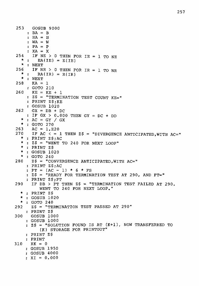
257
253 GOSUB 9000
BA = B
HA = H
WA = W
PA = P
XA = X
254 IF NE > 0 THEN FOR IE = 1 TO NE*
: EA(IE) = E(IE)*
: NEXT
256 IF NR > 0 THEN FOR IR = 1 TO NR*
: RA(IR) = R(IR)*
: NEXT
258 KA = 1
: GOTO 210
260 KE = KE + 1
: Z$ = "TERMINATION TEST COUNTKE="
: PRINT Z$;KE
: GOSUB 1020
262 GX - DB + DC
: IF GX > 0.000 THEN GY = DC + DD*
: AC = GY / GX*
: GOTO 270
263 AC = 1.E20
270 IF AC < = 1 THEN Z$ = "DIVERGENCE ANTICIPATED,WITHAC="
*: PRINT Z$;AC
*: Z$ = "WENT TO 24 0 FOR NEXT
LOOP"
*: PRINT Z$
*: GOSUB 1020
*: GOTO 240
280 Z$ = "CONVERGENCE ANTICIPATED,WITHAC="
PRINT Z$;AC
FT = (AC - 1) * 6 * FS
Z$ = "READY FOR TERMINATION TEST AT 29 0, ANDFT="
PRINT Z$;FT
290 IF DB > FT THEN Z$ = "TERMINATION TEST FAILED AT 290.
WENT TO 240 FOR NEXTLOOP."
*: PRINT Z$
*: GOSUB 1020
*: GOTO 240
292 Z$ = "TERMINATION TEST PASSED AT290"
: PRINT Z$
300 GOSUB 1000
: GOSUB 1000
: Z$ = "SOLUTION FOUND IS AT (K+l), NOW TRANSFERRED TO
(K) STORAGE FORPRINTOUT"
: PRINT Z$
310 KK = 0
: GOSUB 1950
: GOSUB 4 0 00
: XI = 0.000
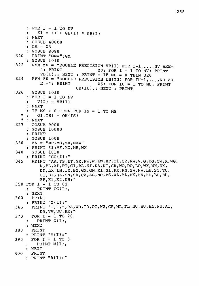
258
320
322
324
326
*
*
327
330
340
345
FOR I = 1 TO NV
XI = XI + GB(I) *GB(I)
NEXT
GOSUB 40600
GM = X3
GOSUB 8080
PRINT "GM=";GM
GOSUB 1010
REM Z$ = "DOUBLE PRECISION VB(I) FOR 1=1,..., NV ARE=
": PRINT Z$: FOR I = 1 TO NV: PRINT
VB(I),: NEXT : PRINT : IF NU = 0 THEN 326REM Z$ = "DOUBLE PRECISION UB(IU) FOR IU=1,...,NU AR
E =": PRINT Z$: FOR IU = 1 TO NU: PRINT
UB(IU) , : NEXT : PRINT
GOSUB 1010
FOR I = 1 TO NV
V(I) = VB(I)
NEXT
IF MS > 0 THEN FOR IS = 1 TO MS
OI(IS) = OK(IS)
NEXT
GOSUB 9000
GOSUB 10000
GOSUB 1000
Z$ ="MF,MG,MR,NX="
PRINT Z$;MF,MG,MR,NX
GOSUB 1010
PRINT "CG(I):"
PRINT "AA,TS,ET,SX,FW,W,LW,BF,C1,C2,RW,V,G,DG,CW,R,WG,
N,PL,AP,FT,CI,BA,NI,NA,NT,CR,WO,DO,LO,WX,WN,DX,
DN,LX,LN,IX,BX,GX,GN,X1,N1,RX,RN,XW,NW,LH,ST,TC,
HI,BI,HA,SN,SA,CA,AG,NC,BS,XL,ML,HX,HN,HD,BD,ED,EP,K1,K2,NH:"
350 FOR I = 1 TO 62
: PRINT CG(I) ,
: NEXT
360 PRINT
: PRINT "Z(I):"
365 PRINT "-,-,-,RA,WD,ID,OC,W2,CP,NL,FL,NU,HU,HL,FU,Al,K5,W,UU,ER:"
370 FOR I = 1 TO 20
: PRINT Z(I),
: NEXT
380 PRINT
: PRINT"M(I):"
390 FOR I = 1 TO 3
: PRINT M(I),
: NEXT
400 PRINT
: PRINT "R(I):"
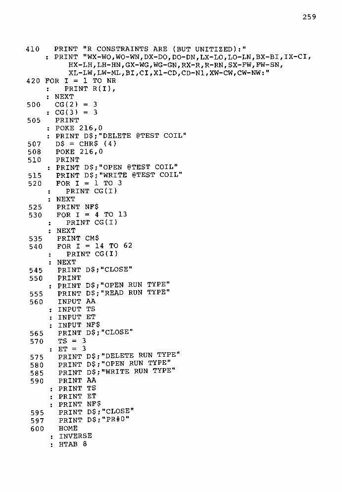
259
410
420
500
505
507
508
510
515
520
525
530
PRINT "R CONSTRAINTS ARE (BUTUNITIZED):"
: PRINT "WX-WO,WO-WN,DX-DO,DO-DN,LX-LO,LO-LN,BX-BI,IX-CI,
HX-LH , LH-HN , GX-WG ,WG-GN , RX-R , R-RN ,SX-FW ,
FW-SN ,
XL-LW, LW-ML ,BI ,CI ,Xl-CD ,CD-Nl , XW-CW , CW-NW :"
FOR I = 1 TO NR
: PRINT R(I) ,
535
540
545
550
555
560
565
570
575
580
585
590
595
597
600
. NEXT
CG(2) = 3
: CG(3) = 3
: POKE 216,0
: PRINT D$; "DELETE @TESTCOIL"
D$ = CHR$ (4)
POKE 216,0
: PRINT D$;"OPEN @TESTCOIL"
PRINT D$; "WRITE @TESTCOIL"
FOR I = 1 TO 3
: PRINT CG(I)
: NEXT
PRINT NF$
FOR I = 4 TO 13
: PRINT CG(I)
: NEXT
62
PRINT CM$
FOR I = 14 TO
PRINT CG(I)
NEXT
PRINT D$;"CLOSE"
PRINT D$;"OPEN RUNTYPE"
PRINT D$;"READ RUNTYPE"
INPUT AA
INPUT TS
INPUT ET
INPUT NF$
PRINT D$;"CLOSE"
TS = 3
ET = 3
PRINT D$; "DELETE RUNTYPE"
PRINT D$;"OPEN RUNTYPE"
PRINT D$; "WRITE RUNTYPE"
PRINT AA
PRINT TS
PRINT ET
PRINT NF$
PRINT D$;"CLOSE-
PRINTD$;"PR#0"
HOME
: INVERSE
: HTAB 8
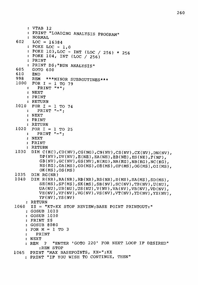
260
: VTAB 12
: PRINT "LOADING ANALYSIS PROGRAM"
: NORMAL
602 LOC = 16384
POKE LOC - 1,0
POKE 103, LOC - INT (LOC / 256) *
POKE 104, INT (LOC / 256)PRINT
PRINT D$;"RUN ANALYSIS"
GOTO 6 00605
610
998
1000
1010
1020
1030
1035
1040
1065
256
END
REM
FOR
NEXT
RETURN
FOR I =
NEXT
RETURN
FOR I =
NEXT
RETURN
DIM
DP
GB
NS
OK
DIM RG
DIM R
SE
UA
***
1 = 1
ii* it
MINOR SUBROUTINES* *-
TO 79
1 TOit_
ii.
1 TOii_n
.
74
25
y[ R(NR),RA(NR),RB(NR) ,RS (NR) , S (MS ) , SA(MS ) , SD (MS ) ,SE(MS) ,SF(MS),SK(MS),SB(NV),SC(NV),TB(NV),U(NU),
UA(NU) ,UB(NU) ,US(NU) ,V(NV) ,VA(NV) ,VB(NV) ,VD(NV) ,
VE(NV) ,VF(NV) ,VG(NV) ,VS(NV) ,VT(NV) , YD (NV) , YE(NV) ,YF(NV) ,YS(NV)
: RETURN
1060 Z$ = "KT=KX STOP REVIEW;BASE POINTPRINTOUT:"
GOSUB 1010
GOSUB 1010
PRINT Z$
GOSUB 8080
FOR M = 1 TO 3
NEXT
REM ? "ENTER 'GOTO220'
FOR NEXT LOOP
:REM STOP
NT "MAX RASEPOINTS. KX=":KX
:REM STOP
PRINT "MAX BASEPOINTS, KX=";KX
PRINT "IF YOU WISH TO CONTINUE,
IFDESIRED"
THEN"
261
1070
1075
1898
1900
*
*
1902
*
*
1905*
*
1910*
*
1920*
*
1930*
;
*:
1940
1948
1950
1960
1965
INPUT "ENTER NEW KX: ";KXIF KX > KT THEN GOTO 22 0
KX = KT
GOTO 1065
REM **NEW BASE POINT ANALYSIS SUBROUTINE 1900-**
FOR I = 1 TO NV
V(I) = VB(I)NEXT
IF MS > 0 THEN FOR IS = 1 TO MS
OI(IS) = OK(IS)
NEXT
GOSUB 9000
QB = QBB = B
HB = H
WB = W
PB = P
XB = X
IF NU > 0 THEN FOR IU = 1 TO NU
UB(IU) = U(IU)
NEXT
IF MS > 0 THEN FOR IS = 1 TO MS
SK(IS) = S(IS)
NEXT
IF NE > 0 THEN FOR IE = 1 TO NE
EB(IE) = E(IE)
NEXT
IF NR > 0 THEN FOR IR = 1 TO NR
RB(IR) = R(IR)
NEXT
IF KG > 0 THEN FOR JG = 1 TO KG
NB(JG) = N(JG)
NEXT
RETURN
REM **MAIN PROGRAM (K) STORAGE INDEX SUBROUTINE 1950:**
DD = DC
DC = DB
FOR I = 1 TO NV
GC(I) = GB(I)
SC(I) = SB(I)
NEXT
QB = QA
BB = BA
HB = HA
WB = WA
PB = PA
XB = XA
FOR I = 1 TO NV
VB(I) = VA(I)
NEXT
IF MS > 0 THEN FOR IS = 1 TO MS
262
* .
*:
* .
1970
*:
*:
1975
*:
*:
1980
*
*
1985
*
*:
*
1990
1998
2000
2001
2002
2003
*
2004
2005
2006
2010
= OA(IS)= SA(IS)
0 THEN FOR
= UA(IU)
0 THEN FOR
= EA(IE)
IU = 1 TO NU
IE = 1 TO NE
IR = 1 TO NR
JG 1 TO KG
OK (IS)
SK(IS)
NEXT
IF NU >
UB(IU)
NEXT
IF NE >
EB(IE)
NEXT
IF NR > 0 THEN FOR
RB(IR) = RA(IR)
NEXT
IF KG > 0 THEN FOR
NC(JG) = NB(JG)
NB(JG) = NA(JG)
NEXT
RETURN
REM ***SUBROUTINE 2000 : SG SEARCH***
KS = 1
XG = 1.E19
CP = AG
PRINT "SG SEARCHFOLLOWS:"
GOSUB 8755
V(l) = CX(1)
V(2) = CX(2)
V(4) =.9
* CN(4) + .1
* CX(4)
V(3) = (.9 * CG(4) + .1
* CG(53)) / CG(4)
IF NV > 4 THEN V(5) =.9
* CN(5) + .1
* CX(5)
V(6) =.9
* CN(6) + .1
* CX(6)
GOSUB 9 000
PRINT"KS,P,Q,V(I)="
PRINT KS,P,Q
FOR I = 1 TO NV
PRINT V(I),
NEXT
XG = X
QG = Q
PG = P
FOR I =
VG(I)
NEXT
SI = 1
FOR I =
RG(I)
NEXT
FOR I = 1 TO NV
V(I)
NEXT
GOSUB 9000
PRINT"KS,V(I),P,Q=
TO NV
V(I)
TO NR
R(D
J. J. \J 1M V
= CN(I) + RND (1) * (CX(I) - CN(I))
263
2020*
*
*
*
*
*
2030
2032
2040
*
2045
*
*
*
*
*
2046
2050
2060
2069
2070
2998
3000
3010
PRINT KS,V(1),P,QPRINT
IF X < XG THEN XG
QG = QPG = P
FOR I = 1 TO NV
VG(I) = V(I)
NEXT
SI = 0
IF KS <
IF PG =
IF KS <
MN THEN 2040
0 AND SI = 0
MX THEN KS =
THEN 2050
KS + 1
GOTO 2010
IF FP < = 1 THEN PRINT "SHOTGUN DID NOT FIND A POINT
WHICH MEETS ALL CONSTRAINTS"
BE PREPARED FOR 6 TO 8 HOUR RUN
... FP
PRINT "SETTING FP=1.TIME"
FP = 1
FOR I = 1 TO NR
PRINT RG(I) ,
NEXT
GOTO 2050
FP = FP / 8
PRINT "FP REDUCED TO
FOR I = 1 TO NR
PRINT RG ( I ) ,NEXT
GOTO 2010
Z$ = "SG SEARCH GAVE FOLLOWINGPOINT:"
PRINT Z$
Z$ ="QG,PG,XG="
PRINT Z$,QG,PG,XG
Z$ = "VG(I) FOR 1=1,..., NVARE="
PRINT Z$
FOR I = 1 TO NV
PRINT VG ( I ) ,
NEXT
A = FRE (0)
FOR I = 1 TO NV
CS(I) = VG(I)
NEXT
RETURN
REM ***SUBROUTINE 3000: SEARCH DIRECTION SB(I),TB(I),
AT VB(I);FOR 1=1 TONV***
GOSUB 4 000
IF ND = 1 OR DC = 0. THEN 3100
264
3015
3020
3030
3040
3050
3060
3090
3100
3150
3160
*
*
3170
3200
3210
3215
*
*
3220*
3230
3240
3250
IF KA > 0 THEN 3100IF ND = 2 OR KG = 0 THEN 3150JG = 1
IF NB(JG) < > NC(JG) THEN 3090IF JG = KG THEN 3150
JG = JG + 1
GOTO 3040
NX = NX + 1
Z$ = "NX,JG="
PRINT Z$,NX,JG
FOR I = 1 TO NV
SB(I) = -
GB(I)NEXT
ID = 1
GOTO 3200
GX = 0.000
GY = GX
FOR I = 1 TO NV
GX = GX + (GB(I) -
GC(I)) *GB(I)
GY = GY + (GB(I) -
GC(I)) * SC ( I )NEXT
IF GY = 0. THEN Z$ = "GY=0. AT 3160; GOTO3100"
PRINT Z$
GOTO 3100
WK = GX / GY
FOR I = 1 TO NV
SB(I) = -
GB(I) + WK *SC(I)
NEXT
ID = 2
PRINT "ID=";ID
DT = 0.000
FOR I = 1 TO NV
DT = DT + GB(I) * SB(I)
NEXT
IF DT < 0. THEN 3240
IF DT = 0. AND ID = 1 THEN Z$ = "STATIONARY POINT FOUND
AT 3215,WITHID,DT="
PRINT Z$;ID,DT
RETURN
IF ID = 2 THEN MR = MR + 1
GOTO 3100
Z$ = "FAILED DESCENT DIRECTION TEST AT 3220,WITHGX="
PRINT Z$;GX
STOP
XI = 0.000
FOR I = 1 TO NV
XI = XI + SB(I)* SB(I)
NEXT
GOSUB 40600
FOR I = 1 TO NV
IF X3 > 0.000 THEN TB ( I ) = SB(I) / X3
265
*: GOTO 3260
3251 TB(I) = 0.000
3260 NEXT
: RETURN
3998 REM ***SUBROUTINE 4000: GRADIENT GB ( I ) AT BASE POINT
VB(I);FOR 1=1 TO NV***
4000 MG = MG + 1
FOR I = 1 TO NV
V(I) = VB(I)
NEXT
IF MS = 0 THEN 4010
4001 FOR IS = 1 TO MS
: OI(IS) = SK(IS)
: NEXT
4010 FOR I = 1 TO NV
4015 IF CD(I) = 0 THEN GB ( I ) = 0*
: NEXT
4020 VT(I) = V(I)
4030 V(I) = VB(I) + CD(I)
: GOSUB 9000
: DP(I) = X
4040 V(I) = VB(I)-
CD(I)
: GOSUB 9000
: DN(I) = X
4050 GB(I) = (DP(I) - DN(I)) / 2 / CD ( I )
4060 V(I) = VT(I)
4070 NEXT
4 08 0 RETURN
4998 REM ***SUBROUTINE 5000:LINE SEARCH FOR (K+l) BASE POINT
- VA(I),I=1 TO NV;AND CP TUNING CALCULATIONS***
5000 REM
5005 IF DT = 0. AND ID = 1 AND KT > 1 AND CP < > 0 . THEN
FR = 0.*
: FB = 0.*
: J = 0
*: GOTO 5230
5010 IF KT = 1 THEN FR = AD
*: GOTO 5040
5015 IF KA > 0 THEN FR = CL * DL
*: GOTO 5040
5020 IF DC = 0. THEN FR = FS / 2
*: GOTO 5040
5 030 IF DC < AD THEN FR = CA * DC
*: GOTO 5040
5031 FR = AD
5040 FB = FR
5050 FOR I = 1 TO NV
: DV(I) = FR * TB(I)
: NEXT
5100 JT = 0
: J = 0
266
TO NV
0.000
VB(I)
THEN 5150
. TO MS
- SK(IS)- OK (IS)- SK(IS)
TO NV
YE(I)
VE(I)
THEN 5160
. TO MS
- OE(IS)- SE(IS)
QD = QB
WD = WB
XD = XB
FOR 1=1
YD(I) =
VD(I) =
NEXT
IF MS = 0
5110 FOR IS = ;
OG(IS) =
OD(IS) =
SD(IS) =
NEXT
5150 QF = QE
WF = WE
XF = XE
FOR 1=1
YF(I) =
VF(I) =
NEXT
IF MS = 0
5155 FOR IS = :
: OF (IS) =
: SF(IS) =
: NEXT
5160 QE = QD
WE = WD
XE = XD
FOR I = 1 TO NV
YE(I) = YD(I)
VE(I) = VD(I)
NEXT
IF MS = 0 THEN 5170
FOR IS = 1 TO MS
OE(IS) = OD(IS)
SE(IS) = SD(IS)
NEXT
JT = JT + 1
J = J + 1
FOR I = 1 TO NV
YD(I) = YE(I) + DV(I)
VD(I) = VB(I) + YD(I)
V(I) = VD(I)
NEXT
IF MS = 0 THEN 5190
5185 FOR IS = 1 TO MS
OD(IS) = OG(IS)
: OI(IS) = OD(IS)
: NEXT
5190 GOSUB 9000
: IF MS = 0 THEN 5192
5165
5170
5180
267
5191 FOR IS = 1 TO MS
SD(IS) = S(IS): OG(IS) = SD(IS): NEXT
5192 MF = MF + 1
: QD = Q: WD = W
: XD = X
5200 IF CP = 0. AND WD > = WE AND WI5205 NN = 0
5210 IF J > = 2 THEN 52605220 IF XD < = XE THEN MC = 1
*: GOTO 5150
5230 GZ = FX * CR
: IF FR < = GZ THEN FOR I = 1 TO*
: VA(I) = VD(I)*
: V(I) = VA(I)*
: NEXT*
: GOTO 5235
5231 GOTO 525 0
5235 IF MS = 0 THEN 5287
5240 FOR IS = 1 TO MS
: OA(IS) = OD(IS): OI(IS) = OA(IS): NEXT
: GOTO 5287
5250 J = 0
: FR = CR * FR
: FOR I = 1 TO NV
: DV(I) = CR *DV(I)
: NEXT
GOTO 5170
5260 IF XD < XE THEN 5350
5270 GX = XD + XF - 2 * XE
IF GX = 0 THEN DS = FR*
; GOTO 5272
5271 DS = FR * (XD -
XE) / GX
5272 XI = 0.000
FOR I = 1 TO NV
XI = XI + YD(I)*YD(I)
NEXT
GOSUB 40600
YJ = X3
YM = YJ - FR / 2 - DS
5280 IF YM < 0.000 THEN Z$ = "FAILED
*: PRINT Z$
*: GOTO 5318
5282 FOR I = 1 TO NV
YS(I) = YM * TB(I)
VA(I) = VB(I) + YS(I)
> 0. THEN 5500
NV
TEST AT5280"
V(I) = VA(I)
268
NEXT
GT = DS + FR / 2
GU = FR * FR
GV = 2 * FR
5284 IF MS = 0 THEN 52875285 FOR IS = 1 TO MS
5286 OU = OD(IS)OV =
OE(IS)OW = OF (IS)GOSUB 5288
OI(IS) = GZ
NEXT
5287 GOSUB 9000
: GOTO 5290
5288 GW = OV - OU
GX = OW - OU
GY = (4 * GW -
GX) / GV
GX = (GW - GY
GW = GT * (GX
GZ = GW + OU
RETURN
5290
5292
*
*
5293
5294
5295*
*
5296* .
* .
5298
*:
*:
5300
5301
5305
5310
*
*
FR) / GU
GT + GY)
MF
QA
BA
HA
WA
PA
XA
MF
QB
H
W
P
X
+ 1
IF NU > 0 THEN FOR IU = 1 TO NU
UA(IU) = U(IU)
NEXT
IF MS = 0 THEN 5295
FOR IS = 1 TO MS
OA(IS) = OI(IS)
SA(IS) = S(IS)
NEXT
IF NE > 0 THEN FOR IE = 1 TO NE
EA(IE) = E(IE)
NEXT
IF NR > 0 THEN FOR IR = 1 TO NR
RA(IR) = R(IR)
NEXT
IF KG > 0 THEN FOR JG = 1 TO KG
NA(JG) = N(JG)
NEXT
IF XA > XB THEN 5305
RETURN
Z$ = "FAILED FUNCTION DECREASE TEST AT 5300"
PRINT Z$
GZ = FX * CR
IF FR > GZ THEN PRINT "WENT TO 5320 AND 5250"
269
*
5312
5314
*
5316*
5318
5319
5320
*
*
*
5322
5350
*
*
*
*
5370
5375*
:
5380
*
5381
GOTO 5320
RETURN
GZ = FX * CR
IF FR > GZ THEN PRINT "WENT TO 5320 FROM5314"
GOTO 5320
IF ABS (YM) > GZ THEN PRINT "WENT TO 5320 FROM5316"
GOTO 5320
FOR I = 1 TO NV
VA(I) = VB(I)
V(I) = VA(I)NEXT
IF MS = 0 THEN 5287
FOR IS = 1 TO MS
OA(IS) = OK(IS)
OI(IS) = OA(IS)
NEXT
GOTO
QE =
WE =
XE =
FOR I =
YE(I)
VE(I)
NEXT
IF MS >
5287
QF
WF
XF
1 TO NV
= YF(I)= VF(I)
0 THEN FOR IS = 1 TO MS
OE(IS) = OF(IS)
SE(IS) = SF(IS)
NEXT
GOTO 5250
IF J > JX THEN Z$
GOSUB 1000
Z$
8080
= "J>JX AT 5350; STOPREVIEW"
GOSUB
STOP
IF FR
IF MC
GOTO
FR =
QE =
WE =
XE =
FOR I =
DV(I)
YE(I)
VE(I)
NEXT
IF MS = 0 THEN MC = 0
GOTO 5382
FOR IS = 1 TO MS
OE(IS) = OF(IS)
SE(IS) = SF(IS)
> FH THEN 5150
< 1 THEN MC = 1
5150
2 * FR
QF
WF
XF
TO NV
2 * DV(I)
YF(I)
VF(I)
270
5382
5500
5501
*:
*
*
5502
*
5510
*
5511
5598
5600
5610
5615
5620
5700
5710
5720
5730
5740
5750
5760
NEXT
MC = 0
GOTO 5150
IF KP > 0 THEN 5502
IF QD > QE THEN NN = 0
Z$ = "IN PENALTY ZONE AT 5500 WITH WD>WE,BUT NO TUNE
SINCEQD>QE"
PRINT Z$
GOTO 5210
IF NN = 0 THEN 5600
REM ***AT FIRST PROBE EDGE OF PENALTY ZONE***
IF KP = 0 THEN KP = 1
GOTO 5150
KP = 2
GOTO 5700
REM ***CP CALCULATION***
REM **SEGMENT 5600 :FOR CP SELF-TUNING PROCESS**
Z$ = "START SEGMENT 5600 - AT EDGE OF PENALTY ZONE WITH
WD>WE ANDQD<QE"
PRINT Z$
FOR I = 1 TO NV
VB(I) = VE(I)
NEXT
IF MS = 0 THEN 5620
FOR IS = 1 TO MS
OK (IS) = OE(IS)
NEXT
GOSUB 19 00
NT = ND
ND = 1
GOSUB 3 000
FB = FR
NN = 1
KP = 0
ND = NT
GOTO 5050
Z$ = "READY FOR CP CALCULATION AT5700"
PRINT Z$
IF WD < > WF THEN CP =.75
* (QF - QD) / (WD - WF)
Z$ = "AT (J-2), ANDKP=0:QF,WF="
PRINT Z$;QF,WF
Z$ = "AT (J-D, ANDKP=1:QE,WE="
PRINT Z$;QE,WE
Z$ = "AT (J), ANDKP=2:QD,WD="
PRINT Z$;QD,WD
Z$ = "REVIEW CALCULATEDCP="
PRINT Z$;CP
FOR M = 1 TO 3
NEXT
PRINT "ENTER GOTO 5790 TO CHANGE CP OR GOTO 58 00 TO
271
5790
5800
5805
5810
*
5815
5820
5830
5840
7997
7999
8000
8010
8020
8030
RETAINCP"
GOTO 5800
REM STOP IS USUALLY HERE
INPUT "ENTER NEW CP=";CP
Z$ = "FOR USE IN SEARCH TO FOLLOW,CP="
PRINT Z$;CP
A = FRE (0)FOR I = 1 TO NV
VB(I) = VE(I)NEXT
IF MS = 0 THEN GOSUB 1900
GOTO 5820
FOR IS = 1 TO MS
OK (IS) = OE(IS)
NEXT
GOSUB 1900
Z$ = "RETURNING TO LINE SEARCH WITH TUNED CP AND NEW
BASE POINT:"
PRINT Z$
GOSUB 1010
GOSUB 8080
NT = ND
ND = 1
GOSUB 3000
FR = AD
NN = 2
ND = NT
FB = FR
GOTO 5050
REM *END OF CP SELF-TUNING PROCESS*
REM * INPUT DATA PRINTOUT*
REM * INPUT DATA PRINTOUT *
Z$ = "AB,AE,AG,AL,AM,AS,ZT,CA,CL,CR,JX,KX="
PRINT Z$
PRINT AB,AE,AG,AL,AM,AS,ZT,CA,CL,CR, JX,KX
Z$ ="KC,KG,MD,MN,MS,MX,ND,NE,NF,NG,NP,NR,NU,NV="
PRINT Z$
PRINT KC,KG,MD,MN,MS,MX,ND,NE,NF,NG,NP,NR,NU,NV
Z$ = "CN(I) FOR 1=1,..., NVARE="
PRINT Z$
FOR I = 1 TO NV
PRINT CN(I) ,
NEXT
Z$ = "CX(I) FOR 1=1,..., NVARE=
PRINT Z$
FOR I = 1 TO NV
PRINT CX(I),
NEXT
i_ ii
272
8040
8045
8050
8052
8055
8057
8060
8061
8068
8070
8072
8078
8080
8090
,NG
ARE="
IF NG = 0 THEN 8050
Z$ = "CG(IG) FOR IG=1,PRINT Z$
FOR IG = 1 TO NG
PRINT CG(IG),NEXT
IF MX > 0 THEN 8060
Z$ = "SPECIFIED CS(I) FOR 1=1,..., NVARE="
PRINT Z$
FOR I = 1 TO NV
PRINT CS(I) ,
NEXT
IF MS = 0 THEN 8060
Z$ = "SPECIFIED OS (IS)PRINT Z$
FOR IS = 1 TO MS
PRINT OS (IS),NEXT
IF KC
Z$ =
FOR IC
FOR IS=1,...,MSARE='
= 0 THEN 8072
CALCULATED CONSTANTS C ( IC )
Z$= 1 TO KC
FOR IC=1,...,KC ARE="
Z$
KT,VB(1),XB,QB
1010
1020
PRINT C(IC) ,
NEXT
GOTO 8072
REM *NP=1,MINIMAL BASE POINT PRINTOUT OPTION*
Z$ ="KT,VB(1),XB,QB="
GOSUB
GOSUB
RETURN
REM *NP=2,FULL BASE POINT PRINTOUT OPTION*
Z$ ="KT,K,XB,QB="
Z$ = "VB(I)
PRINT Z$
FOR I = 1 TO NV
PRINT VB(I),
NEXT
Z$
KT,K,XB,QB
FOR 1=1,..., NVARE='
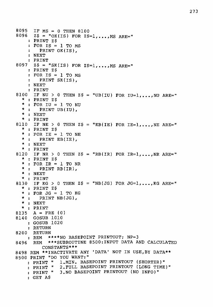
273
8095 IF MS = 0 THEN 8100
8096 Z$ = "OK (IS) FOR IS=1,...,MSARE="
PRINT Z$
FOR IS = 1 TO MS
PRINT OK (IS),NEXT
8097 Z$ = "SK(IS) FOR IS=1,...,MSARE="
PRINT Z$
FOR IS = 1 TO MS
PRINT SK(IS) ,NEXT
8100 IF NU > 0 THEN Z$ = "UB(IU) FOR IU=1,...,NUARE="
*: PRINT Z$
*: FOR IU = 1 TO NU
*: PRINT UB(IU) ,
*: NEXT
8110 IF NE > 0 THEN Z$ = "EB(IE) FOR IE=1,...,NEARE="
*: PRINT Z$
*: FOR IE = 1 TO NE
*: PRINT EB(IE) ,
*: NEXT
8120 IF NR > 0 THEN Z$ = "RB(IR) FOR IR=1,...,NRARE="
*: PRINT Z$
*: FOR IR = 1 TO NR
*: PRINT RB(IR) ,
*: NEXT
8130 IF KG > 0 THEN Z$ = "NB(JG) FOR JG=1,...,KGARE="
*: PRINT Z$
*: FOR JG = 1 TO KG
*: PRINT NB(JG) ,
*: NEXT
8135 A = FRE (0)
8140 GOSUB 1010
: GOSUB 1020
: RETURN
82 00 RETURN
: REM ****NO BASEPOINT PRINTOUT; NP=3
84 96 REM ***SUBROUTINE 8500 .-INPUT DATA AND CALCULATED
CONSTANTS***
8 498 REM ** INACTIVATE ANY'DATA'
NOT IN USE, BY DATA**
8500 PRINT "DO YOUWANT:"
PRINT"
l.MIN. BASEPOINT PRINTOUT (SHORTER)"
PRINT"
2. FULL BASEPOINT PRINTOUT (LONG TIME)"
PRINT"
3. NO BASEPOINT PRINTOUT (NO INFO)"
GET A$
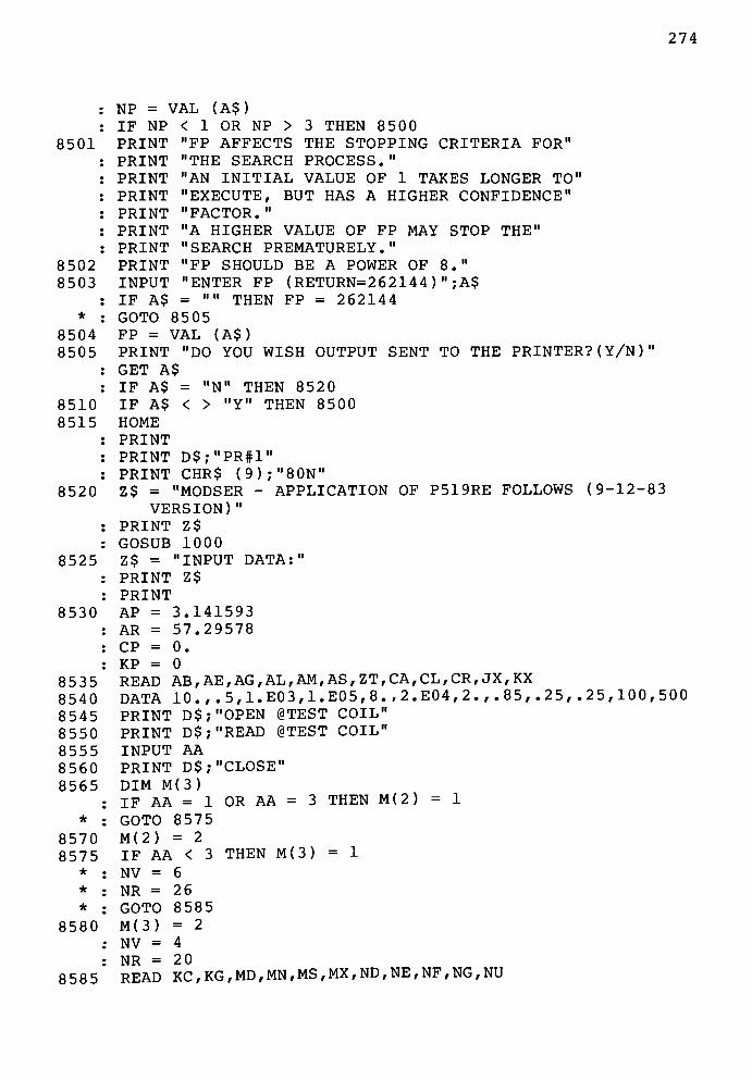
274
8501
8502
8503
*
8504
8505
8510
8515
8520
8525
8530
8535
8540
8545
8550
8555
8560
8565
*
8570
8575
*
*
*
8580
NP = VAL (A$)
IF NP < 1 OR NP >
"FP AFFECTS
"THE SEARCH
"AN INITIAL
INPUT
IF A$
GOTO
3 THEN 8500
THE STOPPING CRITERIAFOR"
PROCESS."
VALUE OF 1 TAKES LONGERTO"
"EXECUTE, BUT HAS A HIGHERCONFIDENCE"
"FACTOR."
"A HIGHER VALUE OF FP MAY STOPTHE"
"SEARCHPREMATURELY."
"FP SHOULD BE A POWER OF8."
"ENTER FP(RETURN=262144)"
;A$
=""
THEN FP = 262144
8505
FP = VAL (A$)
PRINT "DO YOU
GET A$
WISH OUTPUT SENT TO THE PRINTER? (Y/N)"
IF A$
IF A$
HOME
<
"N"THEN 8520
>"Y"
THEN 8500
D$;"PR#1"
CHR$(9);"80N"
Z$ = "MODSER - APPLICATION OF P519RE FOLLOWS (9-12-83
VERSION)"
PRINT Z$
GOSUB 1000
Z$ = "INPUTDATA:"
PRINT Z$
AP = 3.141593
AR = 57.29578
CP = 0.
KP = 0
READ AB,AE,AG,AL,AM,AS,ZT,CA,CL,CR,JX,KX
DATA 10.,.5,1.E03,1.E05,8.,2.E04,2.,.85,.25,.25,100,500
PRINT D$;"OPEN @TESTCOIL"
PRINT D$;"READ @TESTCOIL"
INPUT AA
PRINT D$;"CLOSE"
DIM M(3)
IF AA = 1 OR AA = 3 THEN M(2) = 1
GOTO 8575
M(2) = 2
IF AA < 3 THEN M(3) = 1
NV = 6
NR = 26
GOTO 8585
M(3) = 2
: NV = 4
: NR = 2 0
8585 READKC,KG,MD,MN,MS,MX,ND,NE,NF,NG,NU
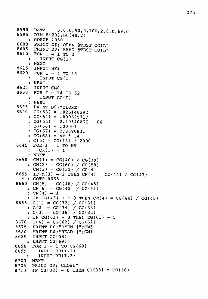
275
8590
8595
8600
8605
8610
8615
8620
8625
8630
8635
8640
8645
8650
8655*
8660
8665
8670
8675
8680
8685
8690
8695
8700
8705
8710
DATA 5,0,0,50,0,100,2,0,0,69,0DIM Z(20),BH(40,2)GOSUB 1030
PRINT D$;"OPEN @TEST COIL"
PRINT D$;"READ @TEST COIL"
FOR I = 1 TO 3
INPUT CG(I)
NEXT
INPUT NF$
FOR I = 4 TO 13
INPUT CG(I)
NEXT
INPUT CM$
FOR I = 14 TO 62
INPUT CG(I)
NEXT
PRINT D$;"CLOSE"
CG(63)
CG(64)
CG(65)
CG(66)
CG(67)
CG(68)
C(5) =
FOR I =
CX(I)
NEXT
CN(1) =
CN(2) =
CN(3) =
IF M(3)
GOTO 8665
CN(5) = CG(46)
CN(6) = CG(42)
CN(4) = 1
IF CG(43) < >
C(l) = CG(32)
C(2) = CG(34)
C(3) = CG(36)
IF CG(61) = 0
C(4) = CG(62)
PRINT D$;"OPEN
=.825146292
=.890525717
= 2.1954066E -
=.00001
= 2.8696831= AP *
.4
CG(13) * 2000
1 TO NV
= 1
06
CG(40) /CG(60) /CG(53) /= 2 THEN
/
/
CG(39)
CG(59)
CG(4)
CN(4) =
CG(45)
CG(41)
CG(44) / CG(43)
0 THEN CN(4) = CG(44) / CG(43)
/ CG(31)
/ CG(33)
/ CG(35)
THEN CG(61) = 5
/ CG(61)
]";CM$
PRINT D$;"READ ]";CM$
INPUT CG(58)
INPUT CG(69)
FOR I = 1 TO CG(69)
INPUT BH(I,1)
INPUT BH(I,2)
NEXT
PRINT D$;"CLOSE"
IF CG(38) = 0 THEN CG(38) = CG(58)
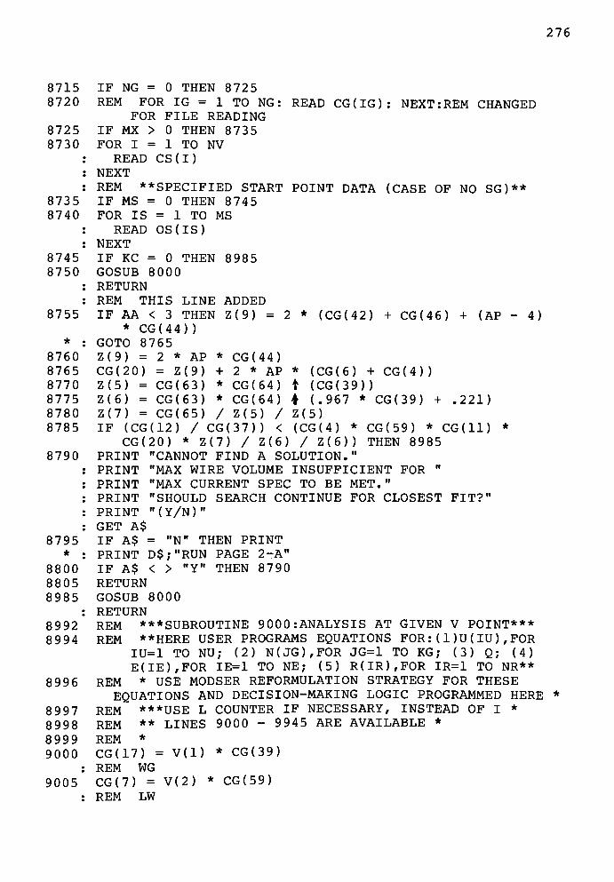
276
8715 IF NG = 0 THEN 8725
872 0 REM FOR IG = 1 TO NG : READ CG(IG): NEXT: REM CHANGED
FOR FILE READING
8725 IF MX > 0 THEN 8735
8730 FOR I = 1 TO NV
READ CS(I)
NEXT
REM **SPECIFIED START POINT DATA (CASE OF NO SG)**
8735 IF MS = 0 THEN 8745
8740 FOR IS = 1 TO MS
: READ OS (IS)
: NEXT
8745 IF KC = 0 THEN 8985
8750 GOSUB 8000
: RETURN
: REM THIS LINE ADDED
8755 IF AA < 3 THEN Z(9) = 2 * (CG(42) + CG(46) + (AP - 4)* CG(44))
*: GOTO 8765
8760 Z(9) = 2 * AP *CG(44)
8765 CG(20) = Z(9) + 2 * AP * (CG(6) + CG(4))
8770 Z(5) = CG(63) * CG(64) t (CG(39))
8775 Z(6) = CG(63) * CG(64) ? (.967 *CG(39) +
.221)
8780 Z(7) = CG(65) / Z(5) / Z(5)
8785 IF (CG(12) / CG(37)) < (CG(4) * CG(59) *CG(ll)
*
CG(20)*Z(7) / Z(6) / Z(6)) THEN 8985
8790 PRINT "CANNOT FIND ASOLUTION."
PRINT "MAX WIRE VOLUME INSUFFICIENT FOR"
PRINT "MAX CURRENT SPEC TO BEMET."
PRINT "SHOULD SEARCH CONTINUE FOR CLOSESTFIT?"
PRINT"(Y/N)"
GET A$
8795 IF A$ ="N"
THEN PRINT
*: PRINT D$;"RUN PAGE
2-A"
8800 IF A$ < >"Y"
THEN 8790
8 805 RETURN
8985 GOSUB 8000
: RETURN
8992 REM ***SUBROUTINE 9000 :ANALYSIS AT GIVEN V POINT***
8994 REM **HERE USER PROGRAMS EQUATIONS FOR: ( 1 )U ( IU ) ,FOR
IU=1 TO NU; (2) N(JG),FOR JG=1 TO KG; (3) Q; (4)
E(IE),FOR IE=1 TO NE; (5) R(IR),FOR IR=1 TO NR**
8996 REM * USE MODSER REFORMULATION STRATEGY FOR THESE
EQUATIONS AND DECISION-MAKING LOGIC PROGRAMMED HERE *
8997 REM ***USE L COUNTER IF NECESSARY, INSTEAD OF I *
8998 REM ** LINES 9000 - 9945 ARE AVAILABLE *
8999 REM *
9000 CG(17) = V(l)* CG(39)
: REM WG
9005 CG(7) = V(2)* CG(59)
: REM LW

277
9010 CG(5) = V(3) *CG(4)
: REM FW
9015 CG(16) = V(4) *CG(43)
: REM R
9020 IF M(3) = 2 THEN 9040
9025 CG(15) = V(5) *CG(45)
: REM CW
9030 CG(14) = V(6) *CG(41)
: REM CD
9035 GOTO 9050
9040 CG(15) = CG(16) * 2
: REM CW
9045 CG(14) = CG(16)* 2
: REM CD
9050 Z(l) = CG(14)- 2 *
CG(16)
9055 Z(2) = CG(15)- 2 * CG(16)
9060 Z(3) = CG(16) + CG(13) / 2
9065 CG(56) = Z(l) * Z(2) + 2 * Z(l) * Z(3) + 2 * Z(2)*
Z(3) + AP * Z(3) * Z(3)
: REM AG
9070 CG(55) = Z(l) * Z(2) + 2 * Z(l)* CG(16) + 2 * Z(2)
* CG(16) + AP * CG(16) * CG(16)
: REM CA
9075 Z(4) = CG(56) / CG(55)
: REM RA
9080 CG(19) = 2 * (CG(7) + 2 * CG(8) + M(2)* CG ( 5 ) + M(2)
* CG(6) + CG(9) + CG(10) + 2 * CG(15))
: REM PL
9085 Z(5) = CG(63)* CG(64) t CG(17)
: REM WD IN CM
9090 Z(6) = CG(63)* CG(64) t (.967 * CG(17) +
.221)
: REM ID IN CM
9095 Z(7) = CG(65) / Z(5) / Z(5)
: REM OC
9100 Z(8) = 1 / Z(6) / Z(6)
: REM W2
9105 IF AA > 2 THEN Z(9) = 2 * AP * CG(16)
*: GOTO 9115
*: REM AP RND
9110 Z(9) = 2 * (CG(14) + CG(15) + (AP - 4) *CG(16))
: REM CP RECT
9115 CG(20) = Z(9) + 2 * AP * (CG(6) + CG ( 5 ) / 2)
: REM AP
9120 CG(18) = CG(ll)* M(2)
* CG(7)*CG(5) *
Z(8)
: REM N
9125 CG(26) = CG(12) / Z(7) / CG(20)
: REM NT
9130 CG(27) = Z(7)* M(2)
* CG(7)*CG(5)
*CG(ll) *
CG(20)
* Z(8)
: REM CR
913 5 REM FIND B-H SEGMENT WHICH STRADDLES THE OPERATING

278
POINT
9140 FOR L = 1 TO CG(69)
9145 CG(24) = CG(19)*BH(L,1) / CG(68)
: REM NI AT SEGMENT END
9150 CG(25) = BH(L,2)*C(5) / Z(4) / CG(68)
: REM NA AT SEGMENT END
9155 IF L = 1 AND (CG(24) + CG(25)) > CG(26) THEN PRINT
"TOO LOW ON B-H CURVE TOANALYZE"
*: PRINT "WILL CONTINUE WITH NI ,NA,BI
*: CG(50) = 0
*: CG(51) = 0
*: CG(24) = 0
*: CG(52) = 0
*: CG(23) = 0
*: CG(25) = 0
*: CG(21) = IE - 5
*: GOTO 9300
*: REM SHOULD HAVE STOPPED, NEED BETTER
9160 IF (CG(24) + CG(25)) > CG(26) THEN 9185
9165 Z(10) = CG(24)
: REM NL
9170 Z(ll) = BH(L,2)* CG(55)
: REM FL
9175 NEXT
9180 PRINT "TOO HIGH ON B-H CURVE TOANALYZE"
: END
9185 Z(12) = CG(24)
: REM NU
9190 Z(13) = BH(L,1)
: REM HU
9195 Z(14) = BH(L - 1,1)
: REM HL
9200 Z(15) = BH(L,2)* CG(55)
: REM FU
9205 M(l) = (Z(15) - Z(1D) / ( LOG (Z(13)) - LOG (Z(14)))
: REM Ml
9210 Z(16) = CG(68)* CG(56) / C(5) / M(l)
: REM Al
9215 Z(17) = Z(16)* CG(26) + LOG (Z(10)) - Z(ll) / M(l)
: REM K5t
9220 Z(18) = Z(17)- Z(16)
* Z(10)- LOG (Z(10))
: REM W
9225 Z(19) = Z(16)* Z(12)
- Z(17) + LOG (Z(12))
: REM UU
9230 CG(24) = (Z(10)* Z(19) + Z(12)
* Z(18)) / (Z(18) +
Z(19))
REM NI
Z(20) = Z(17)- Z(16)
* CG(24)- LOG (CG(24))
: REM ER
9240 IF ABS (Z(20)) < CG(66)* CG(24) THEN GOTO 9270
9245 ON ( SGN (Z(20) + 2)) GOTO 9250,10,9260
279
9250 Z(12) = CG(24)
: REM NU
9255 GOTO 9220
9260 Z(10) = CG(24)
: REM NL
9265 GOTO 9220
9270 CG(50) = CG(24) *CG(68) / CG(19)
: REM HI
9275 CG(51) = ((Z(15) -
Z(ll)) * (CG(50) - Z(14)) / (Z(13)-
Z(14)) + Z(ll)) / CG(55)
: REM BI
9280 CG(23) = CG(51) / Z(4)
: REM BA
9285 CG(52) = CG(23)
: REM HA IN KILO-OERSTEDS
9290 CG(25) = CG(52) *C(5) / CG(68)
: REM NA
9295 CG(21) = CG(23) *CG(23) * CG(56) * CG(67)
: REM FT
9300 Q = 1 / CG(21)
9305 CG(47) = CG(18) * CG(27) * CG(23) * CG(56) / CG(12)
/ 100000
: REM LH
9310 CG(54) = M(2)* CG ( 7 ) * (CG(20) + AP * CG ( 5 ) )
: REM SA
9315 CG(28) = 2 * (CG(15) + M(2)* CG ( 6 ) + M(2)
* CG ( 5 ) )
+ CG(10)
: REM WO
9320 CG(29) = 2 * (CG(6) + CG(5)) + CG(14)
: REM DO
9325 CG(30) = 2 * (CG(15) + CG(8)) + CG(7) + CG(9)
: REM LO
9330 CG(22) = CG(12) / CG(27)
: REM CI
9335 CG(48) = 0
: REM ST
9340 CG(49) = 0
: REM TC
9345 R(l) = 1 - CG(28) / CG(31)
9350 R(2) = CG(28) / CG(31)- C(l)
9355 R(3) = 1 - CG(29) / CG(33)
9360 R(4) = CG(29) / CG(33)- C(2)
9365 R(5) = 1 - CG(30) / CG(35)
9370 R(6) = CG(30) / CG(35)- C(3)
9375 R(7) = 1 - CG(51) / CG(38)
9380 R(8) = 1 - CG(22) / CG(37)
9385 R(9) = 1 - CG(47) / CG(61)
9390 R(10) = CG(47) / CG(61)- C(4)
9395 R(ll) = 1 - V(l)
9400 R(12) = V(l)- CN(1)
9405 R(13) = 1 - V(4)
280
9410
9415
9420
9425
9430
9435
9440
9445
9450
9455
9460
9465
9470
9475
9946
9947
9948
9949
9950
9960
9970
9980
9982
9990
9994
9996
9998
10000
10001
R(14) =
R(15) =
R(16) =
R(17) =
R(18) =
R(19) =
R(20) =
IF M(3)
R(21) =
R(22) =
R(23) =
R(24) =
R(25) =
R(26) =
REM
REM
REM
REM
B =
H =
IF
V(4) -
CN(4)1 -
V(3)
V(3) -
CN(3)1 "
V(2)
V(2) -
CN(2)
CG(51) / CG(38)
CG(22) / CG(37)= 2 THEN 9949
1 -
V(6)
V(6) -
CN(6)
1 -
V(5)
V(5) -
CN(5)
1
1
- 2
- 2
CG(16)
CGQ6)*
**
***
***
0.
0.
NE = 0
CG(15)
CG(14)
DO NOT ALTER LINES 9950 - 9990
THEN 9970
E(IE)
H = H + R(IR) *R(IR)
FOR IE = 1 TO NE
B = B + E(IE) *
NEXT
IF NR = 0 THEN 9990
FOR IR = 1 TO NR
IF R(IR) < 0. THEN
NEXT
W = B + H
P = CP * FP * W
X = Q + P
RETURN
REM ***SUBROUTINE 10000 :FINAL ITEMS ***
REM ** HERE USER PROGRAMS FINAL ITEMS OF INTEREST, BY
F(JF) EQUATIONS, FOR JF=1 TO NF **
* t.tmpc 10010 - 10980 ARE "ati
RETURN
AVAILABLE
10007
10008
10009
10989
10990
10991
10992
REM * LINES
IF NF = 0 THEN
GOSUB 1010
ZF$ = "FINAL ITEMS F(JF) FOR JF=1,...,NF ARE=
PRINT ZF$
REM
i_ n
REM
REM
REM
REM
REM
FOR
***
**
*
*
**
***
JF = 1 TO NF
PRINT F(JF),
NEXT
RETURN
40020 REM *****P518 - TRS-80 DOUBLE PRECISION SUBROUTINES
281
FOLLOW FOR REST OF PROGRAM P519RE*****
4 0040 REM RESERVED VARIABLE NAMES ARE XI ,Xl ,X2 ,X3 ,X4 ,X9 , II ,
10,11,11 AND 13
40594 REM ***SQUARE ROOT***
40600 X3 = SQR (XI)
: IF X3 = 0.000 THEN RETURN
40601 X3 = (X3 + XI / X3) / 2
: RETURN

282
PROGRAM LENGTH IS 19642 ($4CBA) BYTES
A 50, 131, 2069, 5805, 8135
A$ 8500, 8505, 8510, 8790, 8795, 8800
AA 560, 590, 8565, 8575, 8755, 9105
AB 50, 53, 8000, 8535
AC 262, 263, 270, 280
AD 50, 55, 70, 5010, 5030, 5031, 5830
AE 53, 8000, 8535
AG 2000, 8000, 8535
AL 40, 8000, 8535
AM 250, 8000, 8535
AP 8530, 8640, 8755, 8760, 8765, 9065, 9070, 9105, 9110,
9115, 9310
AR 8530
AS 50, 53, 8000, 8535
B 130, 253, 1902, 5290, 9950, 9960, 9990
BA 253, 1960, 5290
BB 130, 1902, 1960
BH( 8695, 9145, 9150, 9170, 9190, 9195, 9200
CA 5030, 8000, 8535
CD( 40, 1030, 4015, 4030, 4040, 4050
CG( 350, 500, 520, 530, 540, 1030, 2002, 8045, 8610, 8620,
8630, 8640, 8650, 8655, 8660, 8665, 8670, 8685, 8690, 8710,
8755, 8760, 8765, 8770, 8775, 8780, 8785, 9000, 9005, 9010,
9015, 9025, 9030, 9040, 9045, 9050, 9055, 9060, 9065, 9070,
9075, 9080, 9085, 9090, 9095, 9105, 9110, 9115, 9120, 9125,
9130, 9140, 9145, 9150, 9155, 9160, 9165, 9170, 9185, 9200,
9210, 9215, 9230, 9235, 9240, 9250, 9260, 9270, 9275, 9280,
9285, 9290, 9295, 9300, 9305, 9310, 9315, 9320, 9325, 9330,
9335, 9340, 9345, 9350, 9355, 9360, 9365, 9370, 9375, 9380,
9385, 9390, 9435, 9440, 9470, 9475
CL 5015, 8000, 8535
CM$ 535, 8625, 8675, 8680
CN( 40, 50, 1030, 2002, 2003, 2010, 8020, 8650, 8655, 8660,
9400, 9410, 9420, 9430, 9455, 9465
CP 70, 222, 240, 2000, 5005, 5200, 5710, 5750, 5790, 5800,
8530, 9990
CR 5230, 5250, 5310, 5314, 8000, 8535
CS( 80, 1030, 2070, 8052, 8730
CX( 40, 50, 1030, 2002, 2003, 2010, 8030, 8645
C( 1030, 8061, 8640, 8665, 8670, 9150, 9210, 9290, 9350,
9360, 9370, 9390
D$ 18, 505, 510, 515, 545, 550, 555, 565, 575, 580, 585,
595, 597, 602, 8515, 8600, 8605, 8635, 8675, 8680, 8705, 8795
DB 190, 195, 200, 262, 290, 1950
DC 70, 262, 1950, 3010, 5020, 5030
DD 262, 1950
DL 70, 195, 5015
DN( 1030, 4040, 4050
DP( 1030, 4030, 4050

283
DS 5270, 5271, 5272, 5282
DT 3210, 3215, 5005
DV( 1030, 5050, 5180, 5250, 5380E 8640
El 2000
E2 263
EA( 254, 1030, 1975, 5295
EB( 110, 1030, 1910, 1975, 8110
ES( 1030
ET 560, 570, 590
E( 110, 254, 1030, 1910, 5295, 9960FB 180, 5005, 5040, 5620, 5830
FD 50, 55
FE 170, 180
FH 50, 55, 5370
FM 52, 53, 55, 224
FP 57, 224, 250, 2045, 2046, 9990
FR 170, 5005, 5010, 5015, 5020, 5030, 5031, 5040, 5050, 5230,5250, 5270, 5271, 5272, 5282, 5288, 5310, 5314, 5370, 5380,5620, 5830
FS 50, 55, 200, 204, 206, 280, 5020
FT 280, 290
FX 50, 55, 204, 206, 5230, 5310, 5314
F( 1030, 10992
GB( 310, 1030, 1950, 3100, 3160, 3170, 3210, 4015, 4050
GC( 1030, 1950, 3160
GM 310, 320
GS( 1030
GT 5282, 5288
GU 5282, 5288
GV 5282, 5288
GW 5288
GX 190, 262, 3150, 3160, 3170, 3230, 5270, 5271, 5288
GY 262, 3150, 3160, 3170, 5288
GZ 5230, 5286, 5288, 5310, 5314, 5316
H 130, 253, 1902, 5290, 9950, 9980, 9990
HA 253, 1960, 5290
HB 130, 1902, 1960
I 40, 50, 80, 190, 252, 310, 326, 350, 370, 390, 420, 520,
530, 540, 1000, 1010, 1020, 1900, 1950, 1960, 2005, 2006, 2010,2020, 2045, 2046, 2060, 2070, 3100, 3160, 3170, 3210, 3240,
3250, 3251, 4000, 4010, 4015, 4020, 4030, 4040, 4050, 4060,
5050, 5100, 5150, 5160, 5180, 5230, 5250, 5272, 5282, 5318,
5320, 5380, 5610, 5810, 8020, 8030, 8052, 8090, 8610, 8620,
8630, 8645, 8690, 8695, 8730
IC 8061
ID 3100, 3170, 3200, 3215, 3220, 5005
IE 110, 254, 1910, 1975, 5285, 8110, 9960
IG 8045
IR 120, 256, 1920, 1980, 5296, 8120, 9980
IS 82, 96, 252, 326, 1900, 1905, 1965, 4001, 5110, 5155,
284
5165,
5615,IT
IU
J
JF
JG
JT
JX
K
KA
KC
KE
KG
KK
KP
KS
KT
KX
L
LO
M
MC
MD
ME
MF
MG
MN
MR
MS
4000,
5190,
5320,
8095,MX
M(
9205,
NA(
NB(
NC(
ND
NE
9950,NF
NF$
NG
NN
NP
NR
2046,
NS(
5185,
5815,70
90, 1
5005,10992
100,
180,
5350,
70, 2
70, 1
1030,
70, 2
100,310
70, 5
2000,
70, 1
210,
9140,602
1060,
5220,
8010,
55, 2
70, 3
70, 3
2030,
70, 3
80, 8
4001,
5191,
5380,
8096,
60, 2
390,
9210,
1030,
100,
1030,
3010,
52, 1
9960
1030,
525,
1030,
70, 5
150,
52, 1
5296,
1030
5191, 5240, 5285, 528
8057, 8096, 8097, 874
902, 1970, 5292, 8100
5100, 5170, 5210, 525
1930, 1985, 3030, 3040
5100, 5170
8000, 8535
20, 230, 240, 8080
95, 258, 3015, 5015
8010, 8060, 8061, 858
60
1030, 1930, 1985, 3020
500, 5510, 5511, 5620,
2005, 2010, 2030, 204
40, 210, 220, 5005, 50
8000, 8535
9145, 9150, 9155, 917
5760
5375
8585
01, 2
30. 5
30, 4
8010
30, 3
2, 95
5100
5235
5381
8097
040,
8565,
9215
1985
1030,
1985
3020
10, 2
5380, 5381
02, 204
192, 52
000
, 8585
220
, 96, 2
, 5110,
, 5240,
, 5610,
, 8585,
8010, 8
8570,
, 9310,
, 5298
1930,
, 3040
, 5620,
54, 103
6, 5294, 5319, 5320, 5381,
0
0, 5350
, 3050, 3060, 3090, 5298, 8130
5, 8745
, 3050, 5298, 8010, 8130, 8585
8530
0
10, 8070, 8080
0, 9190, 9195, 9200
230, 206, 222,
90
52, 326, 1030, 1040, 1900, 1905, 1965,
5150, 5155, 5160, 5165, 5180, 5185,
5284, 5285, 5293, 5294, 5318, 5319,
5615, 5810, 5815, 8010, 8055, 8057,
8735, 8740
050, 8585, 8725
8575, 8580, 8655, 9020, 9080, 9120, 9130,
9315, 9445
1985, 3040, 8130
5830, 801
0, 1910, 1
8010, 8585, 10000, 10
560, 590, 8615
8010, 8040, 8045, 858
205, 5501, 5502, 5620,
8010, 8500
20, 256, 420, 1035, 10
8010, 8120, 8575, 858
0, 8585
975, 5295, 8010, 8110, 8585,
992
5, 8715
5830
40, 1920, 1980, 2006, 2045,0, 9970, 9980
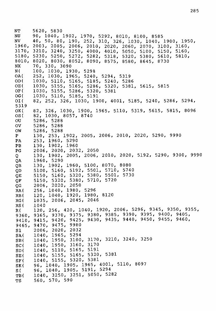
285
NT
NU
NV
1960,
3170,
5180,
8010,NX
N(
OA(
OD(
OE(
OF(
OG(
OI(
5319
OK(
OS(
OU
OV
OW
P
PA
PB
PG
QQA
QB
QD
QE
QF
QG
RA(
RB(
RG(
RS(
R(
9360,
9410,
9465,
SI
SA(
SB(
SC(
SD(
SE(
SF(
SK(
S(
TB(
TS
5620, 5830
90, 1040, 1902, 1970, 5292, 8010, 8100, 8585
40, 50, 80, 190, 252, 310, 326, 1030, 1040, 1900, 1950,
2003, 2005, 2006, 2010, 2020, 2060, 2070, 3100, 3160,
3210, 3240, 3250, 4000, 4010, 5050, 5100, 5150, 5160,
5230, 5250, 5272, 5282, 5318, 5320, 5380, 5610, 5810,
8020, 8030, 8052, 8090, 8575, 8580, 8645, 8730
70, 330, 3090
100, 1030, 1930, 5298
252, 1030, 1965, 5240, 5294, 5319
1030, 5110, 5165, 5185, 5240, 5286
1030, 5155, 5165, 5286, 5320, 5381, 5615, 5815
1030, 5155, 5286, 5320, 5381
1030, 5110, 5185, 5191
82, 252, 326, 1030, 1900, 4001, 5185, 5240, 5286, 5294,
82, 3
82, 1
5286,
5286,
5286,
130,
253,
130,
2006,
130,
1960,
130,
5100,
5150,
5150,
2006,
256,
120,
1035,
1040
120,
9365,
9415,
9470,
2006,
1040,
1040,
1040,
1040,
1040,
1040,
96, 1
96, 1
1040,
560,
26, 1030,
030, 8057
5288
5288
5288
253, 1902
1960, 529
1902, 196
2020, 20
1902, 200
5290
1902, 196
5160, 51
5160, 53
5320, 53
2020, 20
1040, 198
1040, 192
2006, 20
1900, 1965, 5110, 5319, 5615, 5815, 8096
, 8740
, 2005, 2006, 2010, 2020, 5290, 9990
0
0
32, 2050
5, 2006, 2010, 2020, 5192, 5290, 9300, 9990
0, 5100, 8070, 8080
92, 5501, 5710, 5740
20, 5380, 5501, 5730
80, 5710, 5720
50
0, 5296
0, 1980, 8120
45, 2046
256,
937
942
947
202
196
195
195
511
515
515
040,
040,
325
570,
420,
0, 93
0, 94
5, 99
0, 20
5, 52
0, 31
0, 31
0, 51
5, 51
5, 53
1905
1905
0, 32
590
1
75
25
80
32
94
00
60
65
65
20
r
51
040, 1920, 2006, 5296, 9345, 9350, 9355,
, 9380, 9385, 9390, 9395, 9400, 9405,
, 9430, 9435, 9440, 9450, 9455, 9460,
, 3170, 3210, 3240, 3250
,3170
,5191
, 5320, 5381
,5381
1965, 4001, 5110, 8097
5191, 5294
, 5050, 5282

286
UA(
UB(
US(
U(
VA(
VB(
5180,
VD(
VE(
VF(
VG(
VS(
VT(
V(
2020,
9000,
9415,W
WA
WB
WD
WE
WF
WK
X
X3
XA
XB
XD
XE
XF
XG
XI
YD(
YE(
YF(
YJ
YM
YS(
Z$
1060,
5501,
8010,
8096,
ZF$
ZT
Z(
9060,
9115,
9200,
9250,
1040,
90, 1
1040
90, 1
190,
80, 1
5282,
1040,
1040,
1040,
1040,1040
1040,
80, 2
4000,
9005,
9420,
130,
253,
130,
5100,
5150.
5150,
3170
130,
190,
253,
130,
5100,
5150,
5150,
2000,
190,
1040,
1040,
1040,5272
5272,
1040,
30, 5
2050,
5600,
8020,
8097,10001
50, 8
370,
9065,
9120,
9205,
9260,
1970, 5292
040, 1902, 1970, 810
040, 1902, 5292
252, 1040, 1960, 523
90, 326, 1040, 1900,5318, 5610, 5810, 8
5100, 5160, 5180, 5
5150, 5160, 5320, 5
5150, 5320, 5380
2006, 2020, 2060, 2070
0
0, 5282, 5318
1960, 4000, 4030, 4040, 5100,
070, 8090
230
380, 5610, 5810
4020, 4060
52, 326, 1040, 1900,
4020, 4030, 4040, 4
9010, 9015, 9025, 9
9425, 9430, 9450, 9
253, 1902, 5192, 529
1960, 5290
1902, 1960, 5100
5160, 5192, 5200, 5
5160, 5200, 5320, 5
5320, 5380, 5710, 5
253,
310,1960
1902
516
516
527
200
310,510
515
515
1902
3250
, 529
, 196
0, 51
0, 52
0, 53
6, 20
3240
0, 51
0, 51
0, 53
, 200
, 527
0, 53
0, 51
92, 5
20, 5
20, 5
20, 2
, 527
60, 5
60, 5
20, 5
6, 202
2, 406
00
00, 53
220, 5
260, 5
380
050
2, 406
180, 5
180, 5
380
5280, 5282, 5316
5282
5, 130, 180, 250, 26
2060, 3090, 3160, 3
5700, 5720, 5730, 5
8030, 8045, 8052, 8
8100, 8110, 8120, 8
000, 8535
8755, 8760, 8765, 87
9070, 9075, 9085, 9
9125, 9130, 9150, 9
9210, 9215, 9220, 9
9275, 9280
2002, 2003, 2005, 2006, 2010,
060, 5180, 5230, 5282, 5318,
030, 9395, 9400, 9405, 9410,
455, 9460, 9465
0, 9990
710, 5740
380, 5730
720
0, 4030, 4040, 5192, 5290, 9990
00, 40601
00, 8070, 8080
260, 5270, 5271
270, 5271, 5320, 5380
00, 40601
272
320, 5380
0, 270, 280, 290, 292, 300, 330,
215, 3230, 5280, 5305, 5350,
740, 5750, 5800, 5820, 8000,
057, 8061, 8070, 8080, 8090,
130, 8520, 8525
70, 8775, 8780, 8785, 9050, 9055,
090, 9095, 9100, 9105, 9110,
165, 9170, 9185, 9190, 9195,
225, 9230, 9235, 9240, 9245,
APPENDIX G
WIRE DATA INFORMATION
G.l Comparison of Calculated and Table Bare Wire Dias
G.2 Comparison of Calculated and Table Ins. Wire Dias
G.3 Comparison of Calculated and Table Wires/sq-in .
G.4 Comparison of Calculated and Table Ohms/ft . . .
G.5 Sample Page of a Standard Wire Table
.288
.289
.290
.291
.292
287

288
COMPARISON OF CALCULATED AND TABLE VALUES FOR BARE WIRE DIA.
( inches )
NO. TABLE CALCULATION CALC-TABLE %
14
15
16
.0641
.0571
.0508
.0640837262
.0570682062
.0508207053
-1.62738143E-05
-3.17937811E-05
2.07052653E-05
-0.03
-0.06
0.04
17
18
19
.0453
.0403
.0359
.0452571450
.0403026515
.0358905476
-4.28549974E-05
2.65150447E-06
-9.45238572E-06
-0.09
0.01
-0.03
20
21
22
.032
.0285
.0253
.0319614556
.0284624982
.0253465866
-3.85443564E-05
-3.75017844E-05
4.65866324E-05
-0.12
-0.13
0.18
23
24
25
.0226
.0201
.0179
.0225717872
.0201007570
.0179002410
-2.82127658E-05
7.56997906E-07
2.41045200E-07
-0.12
0.00
0.00
26
27
28
.0159
.0142
.0126
.0159406250
.0141955365
.0126414903
4.06249892E-05
-4.46350168E-06
4.14903116E-05
0.29
-0.03
0.33
29
30
31
.0113
.01
.0089
.0112575722
.0100251576
.0089276606
-4.24277714E-05
2.51575802E-05
2.76606443E-05
-0.38
0.25
0.31
32
33
34
.008
.0071
.0063
.0079503114
.0070799568
.0063048836
-4.96886059E-05
-2.00432441E-05
4.88356272E-06
-0.62
-0.28
0.08
35
36
37
.0056
.005
.0045
.0056146610
.0049999999
.0044526286
1.46609582E-05
-2.54658516E-11
-4.73714354E-05
0.26
-0.00
-1.05
38
39
40
.004
.0035
.0031
.0039651802
.0035310950
.0031445309
-3.48197573E-05
3.10949790E-05
4.45308888E-05
-0.87
0.89
1.44
41
42
43
44
.0028
.0025
.0022
.002
.0028002856
.0024937264
.0022207275
.0019776149
2.85624083E-07
-6.27363716E-06
2.07274570E-05
-2.23850893E-05
0.01
-0.25
0.94
-1.12

289
COMPARISON OF CALCULATED AND TABLE INSULATED WIRE DIAMETERS
(inches)
NO. TABLE CALCULATION CALC-TABLE
14
15
16
.0659
.0587
.0524
.0658996273
.0589102805
.0526622273
-3.72703653E-07
2.10280487E-04
2.62227259E-04
-0.00
0.36
0.50
17
18
19
.0469
.0418
.0373
.0470768456
.0420838523
.0376204183
1.76845599E-04
2.83852292E-04
3.20418287E-04
0.38
0.68
0.86
20
21
22
.0334
.0298
.0266
.0336303783
.0300635239
.0268749718
2.30378282E-04
2.63523871E-04
2.74971782E-04
0.69
0.88
1.03
23
24
25
.0239
.0213
.019
.0240245991
.0214765383
.0191987262
1.24599108E-04
1.76538342E-04
1.98726171E-04
0.52
0.83
1.05
26
27
28
.017
.0153
.0137
.0171624999
.0153422367
.0137150316
1.62499855E-04
4.22367048E-05
1.50315645E-05
0.96
0.28
0.11
29
30
31
.0123
.0109
.0097
.0122604086
.0109600636
.0097976339
-3.95914067E-05
6.00636449E-05
9.76339179E-05
-0.32
0.55
1.01
32
33
34
.0088
.0078
.007
.0087584921
.0078295621
.0069991549
-4.15079376E-05
2.95621085E-05
-8.45095201E-07
-0.47
0.38
-0.01
35
36
37
.0062
.0056
.005
.0062568211
.0055932196
.0049999999
5.68211108E-05
-6.78040851E-06
-1.63709046E-11
0.92
-0.12
-0.00
38
39
40
.0045
.0039
.0035
.0044696975
.0039956392
.0035718598
-3.03024681E-05
9.56392223E-05
7.18597639E-05
-0.67
2.45
2.05
41
42
43
44
.0031
.0028
.0025
.0022
.0031930266
.0028543726
.0025516365
.0022810086
9.30265697E-05
5.43726028E-05
5.16364471E-05
8.10086322E-05
3.00
1.94
2.07
3.68

290
14 230
15 290
16 365
17 455
18 572
19 715
20 896
21 1126
22 1413
COMPARISON OF CALCULATED TO TABLE WIRES PER SQUARE INCH
NO. TABLE CALCULATION CALC-TABLE
230.2683 .2682621
288.1495 -1.8505342
360.5799 -4.4200666
451.2168 -3.7831706
564.6366 -7.3634012
706.5660 -8.4339597
884.1715 -11.8285339
1106.4205 -19.5794573
1384.5351 -28.4649134
23 1751 1732.5577 -18.4423227
24 2204 2168.0607 -35.9393024
25 2770 2713.0336 -56.9664068
26 3460 3394.9932 -65.0068178
27 4272 4248.3730 -23.6269817
28 5328 5316.2620 -11.7379875
29 6610 6652.5801 42.5801010
30 8417 8324.8008 -92.1992493
31 10628 10417.3579 -210.642143
32 12913 13035.9089 122.908943
33 16437 16312.6701 -124.329918
34 20408 20413.0918 5.0918121
35 26015 25544.2128 -470.787193
36 31888 31965.1141 77.1141358
37 40000 40000.0003 .0002441
38 49383 50054.5695 671.569443
39 65746 62636.4975 -3109.50253
40 81633 78381.0723 -3251.92767
41 104058 98083.2698 -5974.73026
42 127551 122737.895 -4813.1048
43 160000 153589.811 -6410.18897
44 206611 192196.795 -14414.2046
0. 12
0. 64
1. 21
0. 83
1. 29
1. 18
1. 32
1. 74
2. 01
1.,05
1. 63
2.,06
1.,88
0.,55
0.,22
0.,64
1.,10
1..98
0..95
0..76
0..02
1,.81
0,.24
0,.00
1,.36
4 .73
3 .98
-5 .74
-3 .77
-4 .01
-6 .98

291
COMPARISON OF CALCULATED TO TABLE OHMS/1000 FT
NO. TABLE CALCULATION CALC-TABLE %
14 2.524 2.525614 1. 61411427E-03 0.06
15 3.181 3.184741 3. 74059938E-03 0.12
16 4.018 4.015884 -2. 11624429E-03 -0.05
17 5.054 5.063936 9. 93592106E-03 0.20
18 6.386 6.385505 -4. 94692475E-04 -0.01
19 8.046 8.051974 5. 97353652E-03 0.07
20 10.13 10.1533512 0.0233511701 0.23
21 12.77 12.8031394 0.0331394486 0.26
22 16.2 16.1444608 -0.055539228 -0.34
23 20.3 20.3577892 0.0577891916 0.28
24 25.67 25.6706982 6. 98238611E-04 0.00
25 32.37 32.3701528 1. 52826309E-04 0.00
26 41.02 40.8180091 -0.201990873 -0.49
27 51.44 51.4705593 0.0305592418 0.06
28 65.31 64.903177 -0.406823039 -0.62
29 81.21 81.8413952 0.631395191 0.78
30 103.7 103.200094 -0.499906033 -0.48
31 130.9 130.132916 -0.767084002 -0.59
32 162 164.094577 2.09457737 1.29
33 205.7 206.919442 1.21944183 0.59
34 261.3 260.920599 -0.379400969 -0.15
35 330.7 329.014801 -1.68519926 -0.51
36 414.8 414.880004 0.0800043344 0.02
37 512.1 523.154027 11.0540268 2.16
38 648.2 659.685049 11.4850485 1.77
39 846.6 831.847488 -14.752512 -1.74
40 1079 1048.94032 -30.0596838 -2.79
41 1323 1322.68932 -0.310681343 -0.02
42 1659 1667.88044 8.88043881 0.54
43 2143 2103.1584 -39.8415966 -1.86
44 2593 2652.03379 59.0337849 2.28

292
oc
UJ
a
a
Ou
3
mi
ui_i
a
in
3*< *
*to CO N- 00 OJ o ,_ CM CO
*in CO r-- CO o> o _ CM CO
fl-
m CO r*- CO O) o _ CM co -<r" " "
'" *~ OJ CM OJ CM OJ OJ CM CM OJ OI CO CO CO CO co CO CO CO CO COd- "*- Tl-
T*
$ w Cc o
o o in n OJ m CO CO CO <t o O CM 00 o r-. CO CO r-. CO m 00 o CO CO co CO O i-
CO <~n CO m r-. o~> CM in o r- CD 1^- OI OJ CO o CO o 00 T CO in LO O r-
CM OJ CO TT m N- CD ?_ h-_ CM_r^ * OI_ CO 5 ^ CO OJ
^7f o oo_ o CO h- CO o in O CO
> Q. CT r- T- ^ in d d ,
"
d oi !_r dOI CM CO t * CO CO o OJ CO o
T_ T- r- OI
CO CO O
5OI o m m CO m CO m
o o CO CO OI oo N- oj TT CD
CO
E
OJ CO in CO OI o OJ ^ OJ CO CD CD r-- T m CO T o o^-1 oi CO in CO CM d oi oi oi oi "t CO d d m CO in <* h- r- r-. o m OJ OJ 00
CM CO in CO CO o CO CO o o r. CO r*- CO tt t * 00 CO
o.OJ CO m CO CO co OJ o 00 o CO o CD CO OJ
,_r <r
2.2
OJ CO in 00 CO o-- OJ
to
OC "* 00 <t CO COOI GO m 00
*CO r- o o N. r- OI -*
(A C m o o CO o r h- OJ CO CD co p * CO OJ h- O) o h- CO r- CO* OJ CO
CSJ CO^7
tn CO CO d oi CO d iri oi ^ -r- in ,_3
co d oi iri , d <t oi 00 d Oi CO OJ CO CO
c S CM CM CO t m CO CO o CO CO o CD CO TTd- r*- CM m ^r oj
0,0 OI OJ CO 5 m CO co p C0_ co_ r-_ in
,_ *" ,~
CI tT co Tf OJ^-
CO m CM.Q
O) d CO d ,_ CO 00 d f^ <r in o o CO CO O) in cn o m OOd-
O) CO ^ CM co o o^"
CM
r^ o OJ in o in o o CO o CO o CM *r ofl-
m o CO r*- 00 "* o in CM h- OJ
^ OJ OJ CO *r in CD CO o OI_ CD o m OI o o co o CM r-- h- 00 O o CO O CM *-
^- T-.-7 oi oT * CD d Oi d * dx:
T *" *~ ^~ CM CO t m CD CO
3 00 o CM h-
CO oTJ-
OI CO t r-. CD o m*
CO "* CO TT CD co *
CM 00 in<3-
O) CO CM CO OJ OJfl-
OI h- o CO Oi r*- TT CO 00 CO o CO o "t OJ m oj
o CD CO r- r- Tf * OJ r l* t CO 5 OJ o> Oi <r Oi m Ol Oi h- CD m CO CO OI
IIm cn oo OJ OJ Oi * O) in CM Oi h-; CO * CO CO OJ *-; ^ ^ p p O p p p O p p p
eg d r^ d -<r CO CO oi 1~ -r- *"
CO
5
CO -f m -* OJ OI CO o CO h- Tj-
CO CD o CO OI o OJ -* 00 CM h- h- CO o CDTl-
CD Oi CO h- CM r- CO o r- -r CJ) h- in *r OJ o Oi 5 r- CO in m 't tT co CO CO Ol OJ
COO
in m ^ -tf co CO CO OJ CM CM O o o o o o o o o o o o o
o o o o o o o o O o o o o o o o o O o o o o o o p o o o o o
O d d d d d d d d d d d d d d d d d d d d d d d d d d d d d d
C
in
CD
o
r--
oo
mo
oimo
OJ 00 COfl-
CO CD OJ CO o o CO r- CO O) r*- CO CO o CM CO o m OJ in ,- CO m cm
0} Eo
z
CO
o oco
o
CO
COo
Oi
CMo
COOJo
COCM
oCMo
cn
o o
in
o
co
o
CM
o
o
o
Ol
oo
CO
oo
r-
oo
i--
oo
CO
oo
moo
in
oo
oo
COoo
COoo
COoo
CMOo
CM OJo oo o
ECO
d d d d d d d d d d d d d d d d d d d d d d d d d d d d d d d
2
c
i
lO
COo
oCOmo
LO
o
OJCO
o
CM
O
h-
coCOo
Oi
CMCO
o
CO
Oi
OI
o
COCMo
COCMo
oOIo
CD
CO
o
CD
CD
O
Oi
o
CO
CO
o
O)
o
CD
O
o
OJ
oo
in
CO
oo
mr
oo
COoo
o>
moo
CO
moooo
CM
oo
CDCOoo
OICOoo
OJ
CMoo
CO
CMoo
CO oCM CMo oo o
d d d d d d d d d d d d d d d d d d d d d d d d d d d d d d d
CD
oooooo
"3-
oo
CO
oo
OJ
oo
OJ
oo5ooo
o
oo
o
oo
O)
ooo
ooo
00
ooo
CDOoo
r-
ooo
ooo
CD
ooo
COooo
mooo
mooo
ooo
ooo
CO
ooo
COooo
OIooo
CMooo
CMooo
CMOoo
CM t-
o oo oo o
d d d d d d d d d d d d d d d d d d d d d d d d d d d d d d d
e
5CD
omo
COomo
CO
m
o
CO
o
p
OimCOo
oCMCOo
in
ooCMO
COin
CM
o
COOJOIo
oCMo
ojr--
o
O)m
o
OI
o
COCM
o
CO
o
oo
o
OJ
00
oo
oCO
oooo
CO
COoo
COmoo
omoo
m
OO
o
oo
mCO
oo
CO
oo
00
CMoo
mCMoo
CM OOI OIo oo o
.2~z
d d d d d d d d d d d d d d d d d d d d d d d d d d d d d d d
co -o
3 -a
<
Tl-
in CO r- 00 Oi oCM w
OIOJ
CO
CM OJmOI
COCM Ol
COCM
Oi
OJoCO CO
OICO
COCO CO
in
COCO
CO
r-.
coCO
CO
cn
COo
5CM co
tj-
APPENDIX H
INITIAL MAGNETIZATION CURVES FOR MATERIALS
The graph shown in this appendix is frequently used in
textbooks on magnetism. The particular source for this
sample is "Permanent MagnetManual"
from the Magnetic
Materials Section of the General Electric Company, Edmore
Michigan.
293

294
(H-a !8) S3SSnV9O1IX-!8-N0li0nQNI 06N181NI

APPENDIX I
SAMPLE OF DISK CATALOG
The sample catalog from the project disk is included in
this appendix to show the use of a prefix before the material
and design files. The purpose of this prefix is to make a
visual scan of the listing quicker when searching for a
particular file type. Normally, the files would not be
arranged in the convenient order shown in this sample.
295
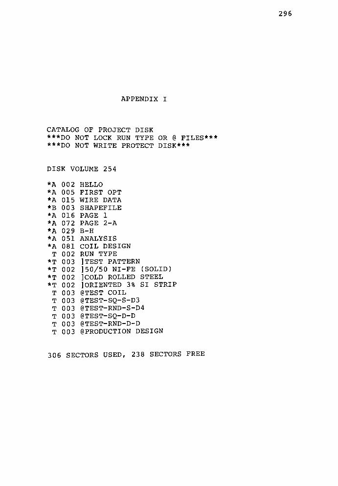
296
APPENDIX I
CATALOG OF PROJECT DISK
***DO NOT LOCK RUN TYPE OR @ FILES***
***DO NOT WRITE PROTECT DISK***
DISK VOLUME 254
*A 002 HELLO
*A 005 FIRST OPT
*A 015 WIRE DATA
*B 003 SHAPEFILE
*A 016 PAGE 1
*A 072 PAGE 2-A
*A 029 B-H
*A 051 ANALYSIS
*A 081 COIL DESIGN
T 002 RUN TYPE
*T 003 ]TEST PATTERN
*T 002 ] 50/50 NI-FE (SOLID)
*T 002 ]COLD ROLLED STEEL
*T 002 jORIENTED 3% SI STRIP
T 003 @TEST COIL
T 003 @TEST-SQ-S-D3
T 003 @TEST-RND-S-D4
T 003 @TEST-SQ-D-D
T 003 @TEST-RND-D-D
T 003 @PRODUCTION DESIGN
3 06 SECTORS USED, 23 8 SECTORS FREE
APPENDIX J
ADDITIONAL COMPUTER TRIALS
J.l TEST-SQ-S-D3 w/COLD ROLLED STEEL CORE 298
J. 2 TEST-SQ-S-D3 w/ORIENTED 3% Si-Strip 302
J. 3 TEST-SQ-S-D5 Optimized with ORIENTED 3% Si-Strip . . .306
J. 4 TEST-SQ-S-D7 Optimized with COLD ROLLED STEEL 310
297
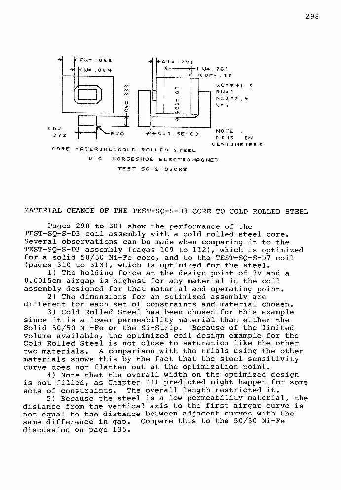
298
-
*-F"
U=.OfeS
tU=. 0 H-
J \
J\.>'
JJ
:
D :
ft = o
* C 1 = . 2 &
li..j=. ?e i
-H K~EF=. 1 5
k- 1 .
ee-o:-
WG a # + 1 5
Rl...l= 1
N= 3 7 .
H-
CORE MftTERIOLsCOLD ROLLED STEEL
D C HORSESHOE ELECTROMAGNET
TE 5 T S 0 S D 3 0 R S
NO TE
D IMS I N
CENTIMETER.?
MATERIAL CHANGE OF THE TEST-SQ-S-D3 CORE TO COLD ROLLED STEEL
Pages 298 to 301 show the performance of the
TEST-SQ-S-D3 coil assembly with a cold rolled steel core.
Several observations can be made when comparing it to the
TEST-SQ-S-D3 assembly (pages 109 to 112), which is optimized
for a solid 50/50 Ni-Fe core, and to the TEST-SQ-S-D7 coil
(pages 310 to 313), which is optimized for the steel.
1) The holding force at the design point of 3V and a
0.0015cm airgap is highest for any material in the coil
assembly designed for that material and operating point.
2) The dimensions for an optimized assembly are
different for each set of constraints and material chosen.
3) Cold Rolled Steel has been chosen for this example
since it is a lower permeability material than either the
Solid 50/50 Ni-Fe or the Si-Strip. Because of the limited
volume available, the optimized coil design example for the
Cold Rolled Steel is not close to saturation like the other
two materials. A comparison with the trials using the other
materials shows this by the fact that the steel sensitivity
curve does not flatten out at the optimization point.
4) Note that the overall width on the optimized design
is not filled, as Chapter III predicted might happen for some
sets of constraints. The overall length restricted it.
5) Because the steel is a low permeability material, the
distance from the vertical axis to the first airgap curve is
not equal to the distance between adjacent curves with the
same difference in gap. Compare this to the 50/50 Ni-Fe
discussion on page 135.
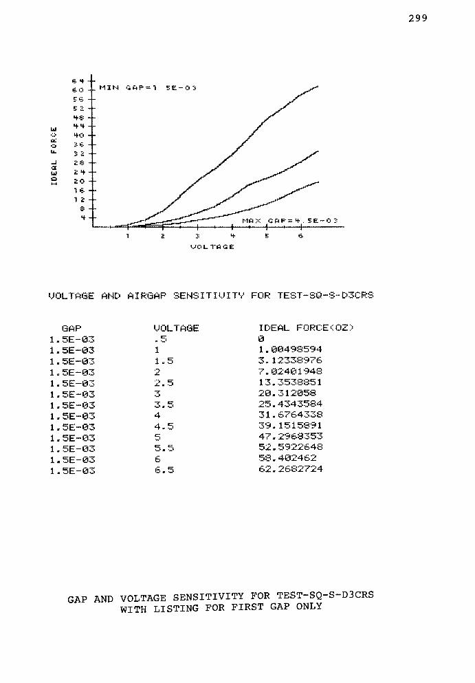
299
Ui
a
e .
-
6-0 - .MIN Gi
5 6 -
E -
HS -
..
-
HO -
~"-
3 J -
2 -
t -
0 -
1 -
1 -
3 -
+ -
lp = 1
VOLTflSE
UOLTAGE AND AIRGAP SENSITIVITY FOR TEST-SQ-S-D3CRS
GAP
, 5E-83
, 5E-83
, 5E-83
, 5E-83
1 . 5E-83
1 . 5E-83
5E-83
5E-03
5E-83
5E-03
5E-03
5E-03
UOLTAGE
1,
1,
1,
1,
1,
1,
1.5E-83
2. 5
3
3.A
5
4. 5
5
5. 5
6
-. 5
IDEAL FORCE <OZ3:
0
1 . 80498594
7.82401948
13.3538851
28.312858
25.4343584
31 . 6764338
39. 1515891
47.2968353
52.5922648
58 . 482462
62 . 2682724
GAP AND VOLTAGE SENSITIVITY FOR TEST-SQ-S-D3CRS
WITH LISTING FOR FIRST GAP ONLY

300
SAMPLE RUN FOR A SINGLE BOBBIN, RECTANGULAR CORE
SUBJECT TO THE STANDARD LIMITS OF THIS PROJECT
COIL NAME:TEST-SQ-S-D3CRS
COIL TYPE: SINGLE BOBBIN, RECTANGULAR CORE
OPERATING VOLTAGE: 3
COIL RESISTANCE: 85. 7314358
CORE MATERIAL : COLD ROLLED STEEL
THEORETICAL, NO LOSS HOLDING FORCE(OZ ): 20 . 312058
EXPECTED HOLDING FORCE (OZ ): 12 . 9997171
****PHYSICAL DIMENSIONS &CONSTANTS****
OVERALL LENGTH: 2. 01084969
OVERALL DEPTH:. 635156443
OVERALL WIDTH: .998625621
FLANGE WIDTH: .0676721706
WINDING LENGTH:. 76056841
BOBBIN WALL THICKNESS :. 064
BOBBIN FLANGE THICKNESS :. 15
ARMATURE/BOBBIN CLEARANCE: . 28 5
WINDING CLEARANCE: .07
AIRGAP :1.5E-03
STEEL PATH LENGTH: 4 . 42504373
CORE WIDTH: .33264064
CORE DEPTH: .371812102
CORNER RADIUS :0
CORE PERIMETER:1. 40890548
CORE AREA: .123679816
AIRGAP AREA (FRINGING) :. 124738262
WINDING SURFACE AREA: 1. 7008 0295
************* *WINDING DATA* *************
WIRE GAGE NUMBER: #41. 4850841
TURNS SPECIFIED:872. 399078
TURNS POSSIBLE:872. 399069
RANDOM WIND:1
WINDING WIDTH: .0676721706
BARE WIRE DIA:6.7237313E-03
OHMS/CM OF WIRE:. 0485617446
EFFECTIVE INSUL.WG : 40 . 3370763
INSULATED WIRE DIA: 7 .68097937E-03
THEORETICAL TURNS/SQ CM=16949 . 8868
CURRENT AT 3 VOLTS :. 0349929985
AVERAGE TURN LENGTH: 2 .02362774
INDUCTANCE, HENRIES:.234257701
S.S.TEMP RISE, DEG C:61. 2650785
ANALYSIS LISTING FOR A COLD ROLLED STEEL CORE IN THE
TEST-SQ-S-D3 COIL ASSEMBLY (CONTINUED ON NEXT PAGE)

301
(SAMPLE LISTING CONTINUED)
THERMAL TIME CONST: 132 . 207211RESISTANCE @S. S. TEMP : 99 . 6594453CURRENT @THAT TEMP :. 0301025155IDEAL FORCE @THAT TEMP @3VOLTS=14 . 6520669************ *MAGNETIC DATA* ************
TOTAL AMP-TURNS ( ACTUAL ):30. 5278593TOTAL AMP-TURNS (AIR+IRON): 30. 2013462AMP-TURNS IN IRON: 12 . 2179572
AMP-TURNS IN AIR: 17 . 9833891
OERSTEDS IN IRON: 3 . 46969177
OERSTEDS IN AIR: 7532 . 86439
KILOGAUSSES IN IRON: 7 . 59733031
KILOGAUSSES IN AIR: 7 . 53286439
IRON SAT KILOGAUSS:20.7********* * *DESIGN CONSTRAINTS ***********
MAX OVERALL LENGTH: 2. 01
MIN OVERALL LENGTH :0
MAX OVERALL DEPTH:. 635
MIN OVERALL DEPTH : 0
MAX OVERALL WIDTH: 1.01
MIN OVERALL WIDTH :0
MAX CORE WIDTH: .5
MIN CORE WIDTH :0
MAX CORE DEPTH : . 5
MIN CORE DEPTH :0
MAX CORE CORNER RAD : 0
MIN CORE CORNER RAD : 0
MAX CURRENT @ 3 VOLTS:. 03 5
MAX WIRE GAGE NUMBER: 45
MIN WIRE GAGE NUMBER: 35
MAX KILOGAUSS IN CORE: 15. 41
DESIGN HINTS:
IF ANY FINAL DIMENSIONS ARE AT OR NEAR
THEIR LIMITS, THEN CHANGING THOSE LIMITS
MAY CHANGE THE FINAL SOLUTION.
TEMPERATURE RISE CAN BE REDUCED BY
INCREASING THE SURFACE AREA (OR LX)
ANALYSIS LISTING FOR A COLD ROLLED STEEL CORE IN THE
TEST-SQ-S-D3 COIL ASSEMBLY (cont)
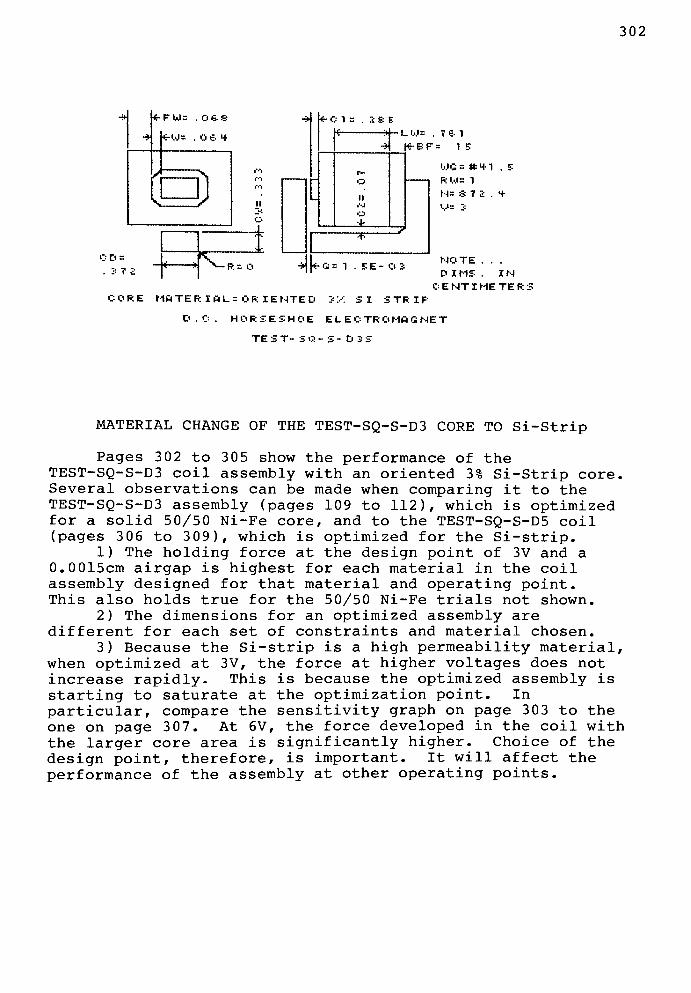
302
-it * FW=. O 6. S
C D :
* fO)=.JSI
L W=. T 6 1
-H (*-BF = 1 E
O
.-
f,G =
RW= 1
N= 3 7 2.4-
'..In ~:
1 . E E - o :NOTE . . .
P IMS. I N
CENTIMETERS
CORE MftTER IfiL=OR IENTED JX SI STRIP
D.C. HORSESHOE E L E C TR O MA G NE T
TEST-Stt-S-D 3S
MATERIAL CHANGE OF THE TEST-SQ-S-D3 CORE TO Si-Strip
Pages 302 to 305 show the performance of the
TEST-SQ-S-D3 coil assembly with an oriented 3% Si-Strip core.
Several observations can be made when comparing it to the
TEST-SQ-S-D3 assembly (pages 109 to 112), which is optimized
for a solid 50/50 Ni-Fe core, and to the TEST-SQ-S-D5 coil
(pages 306 to 309), which is optimized for the Si-strip.
1) The holding force at the design point of 3V and a
0.0015cm airgap is highest for each material in the coil
assembly designed for that material and operating point.
This also holds true for the 50/50 Ni-Fe trials not shown.
2) The dimensions for an optimized assembly are
different for each set of constraints and material chosen.
3) Because the Si-strip is a high permeability material,
when optimized at 3V, the force at higher voltages does not
increase rapidly. This is because the optimized assembly is
starting to saturate at the optimization point. In
particular, compare the sensitivity graph on page 303 to the
one on page 307. At 6V, the force developed in the coil with
the larger core area is significantly higher. Choice of the
design point, therefore, is important. It will affect the
performance of the assembly at other operating points.
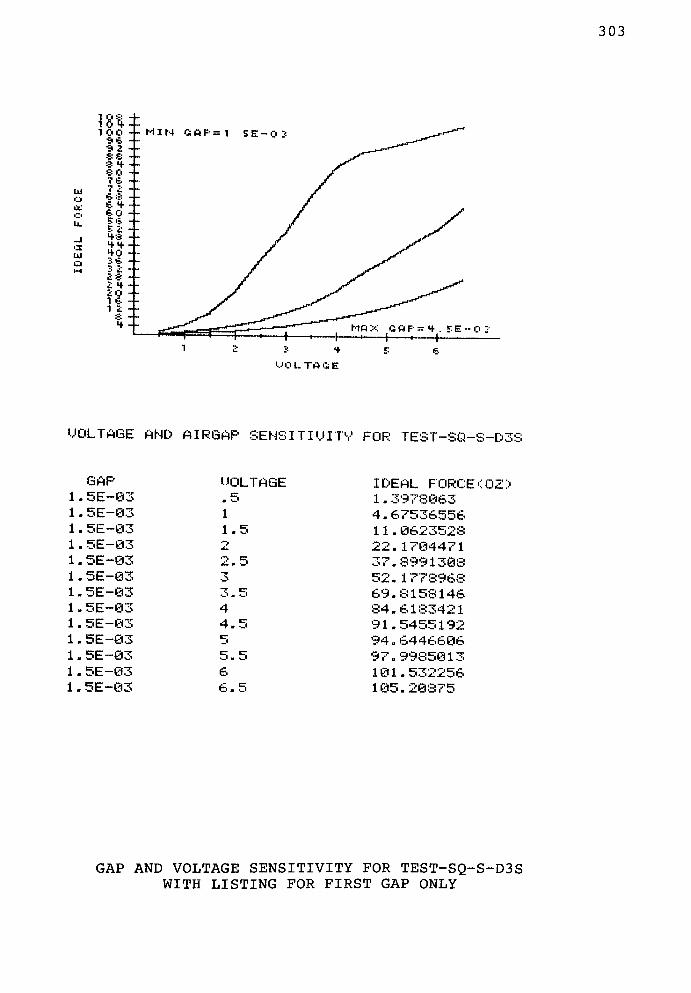
303
o
IX
_l
Iii
a
MOLTflCE
UOLTAGE AND AIRGAP SENSITIUITY FORTEST-SQ-S-D3"
GAP
1 . 5E-83
1 . 5E-03
1 . 5E-03
1 . 5E-03
1 . 5E-83
1 . ^-*E Wo
1 . 5E-83
1 . 5E-83
5E-83
5E-83
5E-83
5E-83
UOLTAGE
1 . 5E-83
3.5
6
6.5
IDEAL FORCE <OZ>
1 . 3978863
4 . 67536556
1 1 . 8623528
22. 1784471
37 . 899 1 388
52. 1778968
69.8158146
84.6183421
91.5455192
94 . 6446686
97.9985813
Iracr">iviO*7?-*s*
Kf-Jm ZOOr -J
GAP AND VOLTAGE SENSITIVITY FOR TEST-SQ-S-D3S
WITH LISTING FOR FIRST GAP ONLY

304
SAMPLE RUN FOR A SINGLE BOBBIN, RECTANGULAR CORE
SUBJECT TO THE STANDARD LIMITS OF THIS PROJECT
COIL NAME:TEST-SQ-S-D3S
COIL TYPE: SINGLE BOBBIN, RECTANGULAR CORE
OPERATING VOLTAGE: 3
COIL RESISTANCE: 85. 7314358
CORE MATERIAL:ORIENTED 3% SI STRIP
THEORETICAL, NO LOSS HOLDING FORCE(OZ ): 52 . 1778968
EXPECTED HOLDING FORCE (OZ ): 33 . 3938539
****PHYSICAL DIMENSIONS &CONSTANTS****
OVERALL LENGTH: 2. 01084969
OVERALL DEPTH:. 635156443
OVERALL WIDTH: .998625621
FLANGE WIDTH:. 0676721706
WINDING LENGTH:. 76 056 841
BOBBIN WALL THICKNESS :. 064
BOBBIN FLANGE THICKNESS :. 15
ARMATURE/BOBBIN CLEARANCE : . 2 8 5
WINDING CLEARANCE: . 07
AIRGAP :1.5E- 03
STEEL PATH LENGTH : 4 . 42504373
CORE WIDTH:. 33264064
CORE DEPTH: .371812102
CORNER RADIUS : 0
CORE PERIMETER:1. 40890548
CORE AREA:. 123679816
AIRGAP AREA ( FRINGING ):. 1247 38262
WINDING SURFACE AREA: 1. 7 0080295
************* *WINDING DATA* *************
WIRE GAGE NUMBER: #41. 4850841
TURNS SPECIFIED:872. 399078
TURNS POSSIBLE:872. 399069
RANDOM WIND:1
WINDING WIDTH: .0676721706
BARE WIRE DIA:6.7237313E-03
OHMS/CM OF WIRE: .0485617446
EFFECTIVE INSUL.WG : 40 . 3370763
INSULATED WIRE DIA: 7 .68097937E-03
THEORETICAL TURNS/SQ CM=16949 . 8868
CURRENT AT 3 VOLTS :. 0349929985
AVERAGE TURN LENGTH: 2 .02362774
INDUCTANCE,HENRIES:.375456994
S.S.TEMP RISE, DEG C:61. 2650785
ANALYSIS LISTING FOR AN ORIENTED 3% Si-STRIP CORE IN THE
TEST-SQ-S-D3 COIL ASSEMBLY (CONTINUED ON NEXT PAGE)

305
(SAMPLE LISTING CONTINUED)
THERMAL TIME CONST: 132 . 207211RESISTANCE @S. S. TEMP : 99 . 6594453CURRENT @THAT TEMP: . 0301025155IDEAL FORCE @THAT TEMP @3VOLTS=40. 3779729*********** *
*MAGNETIC DATA* ************
TOTAL AMP-TURNS (ACTUAL ):30. 5278593TOTAL AMP-TURNS (AIR+IRON): 30. 02 9 5467AMP-TURNS IN IRON: 1 . 20663438AMP-TURNS IN AIR: 28 . 8229124OERSTEDS IN IRON: . 342663616OERSTEDS IN AIR: 12073 . 3133
KILOGAUSSES IN IRON: 12 . 1766362
KILOGAUSSES IN AIR: 12 . 0733133IRON SAT KILOGAUSS:19.7
***********DESIGN CONSTRAINTS***********
MAX OVERALL LENGTH: 2. 01
MIN OVERALL LENGTH : 0
MAX OVERALL DEPTH:. 635
MIN OVERALL DEPTH :0
MAX OVERALL WIDTH: 1.01
MIN OVERALL WIDTH : 0
MAX CORE WIDTH: .5
MIN CORE WIDTH :0
MAX CORE DEPTH : . 5
MIN CORE DEPTH :0
MAX CORE CORNER RAD:0
MIN CORE CORNER RAD:0
MAX CURRENT @ 3 VOLTS:. 035
MAX WIRE GAGE NUMBER: 45
MIN WIRE GAGE NUMBER: 35
MAX KILOGAUSS IN CORE: 15. 41
DESIGN HINTS:
IF ANY FINAL DIMENSIONS ARE AT OR NEAR
THEIR LIMITS, THEN CHANGING THOSE LIMITS
MAY CHANGE THE FINAL SOLUTION.
TEMPERATURE RISE CAN BE REDUCED BY
INCREASING THE SURFACE AREA (OR LX)
***Note: Strip stock is usually available in sheet form and
used to make laminated cores, which would require
the use of a stacking factor. It has been treated
as a solid core, for this example only, to show the
effects of using a higher permeability material than
that used during the optimization process.
ANALYSIS LISTING FOR AN ORIENTED 3% Si-STRIP CORE IN THE
TEST-SQ-S-D3 COIL ASSEMBLY (cont)
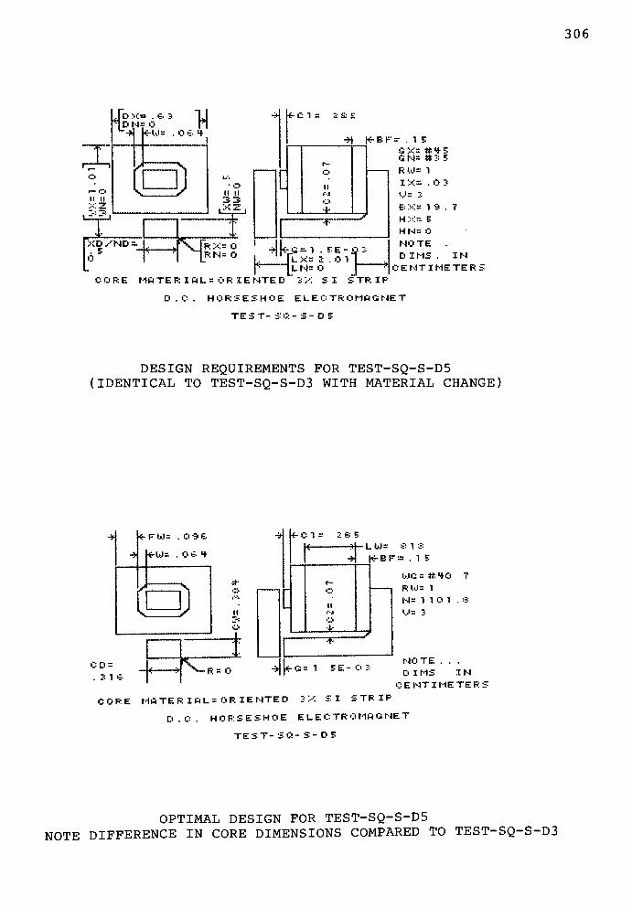
306
*| D N= O n
Xi o
II II
/*
XD /ND :
oe .
i
}) ii n
33
Rrx=oRN=0
I-
ci= s a e
O
II
k.G=1 . EE-O
ft- X= Oil|ln=o
_f
G X= # t EGN=#! 5
RW= 1
I X= . O 3
V 3:
BX= 1 9 . T
HX= E
HN=0
NOTE
D IMS . I N
CENTIMETERS
C O R E Mfi TE ft I fl L = C R I E NTE D 3 X SI STRIP
D.C. HORSESHOE E L E C TR O MB GNE T
TEST-SC-S-O E
DESIGN REQUIREMENTS FOR TEST-SQ-S-D5
(IDENTICAL TO TEST-SQ-S-D3 WITH MATERIAL CHANGE)
<r
<r-W= .OtH
J X
J\ s
CD =
CORE
;*c
o
ft = o
.
:&
E
LW= S 1 S
|fBF=. 1 E
WG = #HO
RW= 1
N= 1 1 01
K--E E - O 3
NOTE . . .
DIMS IN
C E NT I ME TE R i
MflTER IftL=OR IENTED 3X SI STRIP
D . C . H O R S E S H O E E L E C TR O MA G NE T
TEST-SO-S-D E
OPTIMAL DESIGN FOR TEST-SQ-S-D5
NOTE DIFFERENCE IN CORE DIMENSIONS COMPARED TO TEST-SQ-S-D3

307
e .
SO7<=-
9 >1 ll
6 3
<=. He. o
Ul Eo Ete
H
ll ft
HO_J -.
X -! ^Ul
-: i^
o ESl-l E H
0
1 ..
\S=
H
MOLTOGE
UOLTAGE AND AIRGAP SENSITIUITV FOR TEST-SQ-S-D5
GAP
1 . 5E-03
1 . 5E-83
1 5E-83
5E-83
5E-03
5E-03
5E-03
5E-83
5E-83
5E-83
5E-83
1 . 5E-83
1 . 5E-03
UOLTAGE
1
1.5
0-. b
4
4. 5
5
5. 5
6
6. 5
IDEAL FORCE< 02 :>
1 . 57290086
5.86184138
1 4 . 9989666
29.9958917
44.5783929
61 .3016876
78.5134833
73.4987443
76 . 7836684
88. 2677319
83.4885739
83.7331885
83 . 9888466
GAP AND VOLTAGE SENSITIVITY FOR TEST-SQ-S-D5,
WITH LISTING FOR FIRST GAP ONLY

308
SAMPLE RUN FOR A SINGLE BOBBIN, RECTANGULAR CORE
SUBJECT TO THE STANDARD LIMITS OF THIS PROJECT
COIL NAME:TEST-SQ-S-D5
COIL TYPE: SINGLE BOBBIN, RECTANGULAR CORE
OPERATING VOLTAGE: 3
COIL RESISTANCE: 85. 71988
CORE MATERIAL: ORIENTED 3% SI STRIP
THEORETICAL, NO LOSS HOLDING FORCE(OZ ): 61. 3016076
EXPECTED HOLDING FORCE (OZ):39. 2330289
****PHYSICAL DIMENSIONS & CONSTANTS****
OVERALL LENGTH: 2. 01039033
OVERALL DEPTH: .635051052
OVERALL WIDTH: .996965227
FLANGE WIDTH: .0957144184
WINDING LENGTH:. 817853934
BOBBIN WALL THICKNESS :- 064
BOBBIN FLANGE THICKNESS :. 15
ARMATURE/BOBBIN CLEARANCE : . 2 8 5
WINDING CLEARANCE : . 0 7
AIRGAP :1.5E- 03
STEEL PATH LENGTH: 4 . 48020949
CORE WIDTH:. 303768195
CORE DEPTH: .315622215
CORNER RADIUS :0
CORE PERIMETER:1. 23878082
CORE AREA: .0958759906
AIRGAP AREA (FRINGING) :. 0968068433
WINDING SURFACE AREA: 1. 83387 069
************* *WINDING DATA* *************
WIRE GAGE NUMBER: #40. 6562092
TURNS SPECIFIED:1101. 79546
TURNS POSSIBLE: 1101. 79547
RANDOM WIND:1
WINDING WIDTH:. 0957144184
BARE WIRE DIA:7.40196674E-03
OHMS/CM OF WIRE:. 0400701271
EFFECTIVE INSUL.WG : 39 . 5355543
INSULATED WIRE DIA: 8 .42900021E-03
THEORETICAL TURNS/SQ CM=14074 . 9827
CURRENT AT 3 VOLTS :. 0349977158
AVERAGE TURN LENGTH: 1 . 94160039
INDUCTANCE,HENRIES: .45272374
S.S.TEMP RISE, DEG C:57. 5778289
ANALYSIS LISTING FOR AN OPTIMIZED COIL ASSEMBLY, TEST-SQ-S-D5
(CONTINUED ON NEXT PAGE)

309
(SAMPLE LISTING CONTINUED)
THERMAL TIME CONST: 181 . 28958RESISTANCE @S. S. TEMP : 98. 4016397CURRENT @THAT TEMP :. 0304872969IDEAL FORCE @THAT TEMP @3VOLTS=49. 0676941************
*MAGNETIC DATA* * ***********
TOTAL AMP-TURNS ( ACTUAL ):38. 5603248TOTAL AMP-TURNS (AIR+IRON) :38. 4332258AMP-TURNS IN IRON : 2 . 97007462AMP-TURNS IN AIR: 35 . 4631512
OERSTEDS IN IRON: . 833065029OERSTEDS IN AIR:14854.77
KILOGAUSSES IN IRON: 14 . 9989939KILOGAUSSES IN AIR: 14. 85477IRON SAT KILOGAUSS:19.7********* * *DES IGN CONSTRAINTS ***********
MAX OVERALL LENGTH: 2. 01
MIN OVERALL LENGTH :0
MAX OVERALL DEPTH:. 635
MIN OVERALL DEPTH : 0
MAX OVERALL WIDTH: 1.01
MIN OVERALL WIDTH :0
MAX CORE WIDTH: .5
MIN CORE WIDTH: 0
MAX CORE DEPTH : . 5
MIN CORE DEPTH :0
MAX CORE CORNER RAD : 0
MIN CORE CORNER RAD : 0
MAX CURRENT @ 3 VOLTS:. 03 5
MAX WIRE GAGE NUMBER: 45
MIN WIRE GAGE NUMBER: 35
MAX KILOGAUSS IN CORE: 19. 7
DESIGN HINTS:
IF ANY FINAL DIMENSIONS ARE AT OR NEAR
THEIR LIMITS, THEN CHANGING THOSE LIMITS
MAY CHANGE THE FINAL SOLUTION.
TEMPERATURE RISE CAN BE REDUCED BY
INCREASING THE SURFACE AREA (OR LX)
***Note: This is an optimized coil assembly, which has the
same physical constraints as the TEST-SQ-S-D3 coil,
but a different core material. The physical
dimensions are different, and the holding force at
3V is higher than when the ORIENTED 3% Si-Strip CORE
is inserted in a TEST-SQ-S-D3 coil (pages 302-305).
ANALYSIS LISTING FOR AN OPTIMIZED COIL ASSEMBLY, TEST-SQ-S-D5
(cont )

310
K-BF=. 1 E
XD/ND=*\jftx-=o
Hr G =1 . E E -
-
JLX= Oil
~[L N= OJ"
G X= # H EGN=3 E
RW= 1
IX= O 3
M= 3
B X= 0.7
H X= E
HN=-0
NOTE . .
D IMS I N
centimeter:
CORE MATER IAL=COLD ROLLED STEEL
D.C. HORSESHOE E L E C TR OMA G NE T
TEST-SCl-S-D 7
DESIGN REQUIREMENTS FOR TEST-SQ-S-D7
(IDENTICAL TO TEST-SQ-S-D3 WITH MATERIAL CHANGE)
fCls.JSS
LW=. 3 & E
K-BF=. 1 E
WSaStO 1
RW= 1
N=1J0 S 1
V= 3
j* G = 1 . EE-ONOTE .
D I MS I N
CENTIMETER:
C O R E MA TE R I A L = C O L D ROLLED STEEL
D C HORSESHOE ELECTROMAGNET
TEST-SC'-S-D 7
OPTIMAL DESIGN FOR TEST-SQ-S-D7
NOTE DIFFERENCE IN CORE DIMENSIONS COMPARED TO TEST-SQ-S-D3
ALSO, FP HAD TO BE SET TO ONE IN THE COIL DESIGN MODULE.

311
HS -
HH - . MIN
HO -
3 is- -
Ul
o
o
b.
E :3-
E H -
X
Ul
ol-H
EG -
1 e. -
1 -
* -
H -
.*IS
MIN G A P = 1 E E - 0
^
MO L TA G E
UOLTAGE AND AIRGAP SENSITIUITV FOR TEST-SQ-S-D7
GAP
5E-83
, 5E-83
, 5E-03
, 5E-03
5E-03
, 5E-03
,5E~83
, 5E-83
, 5E-83
, 5E-83
, 5E-83
, 5E-83
UOLTAGE
.5
1
1.5
1 . 5E-83
4.5
5ar cr
6
6.5
IDEAL FORCE <0Z>
8
1 . 79838828
5.65883918
1 1 . 8278932
16.4988393
22.6685943
29. 843669
33.9316442
37 - !ii2942ot>
39 . 7788835
42.4679575
44 . 284247
44.6325183
GAP AND VOLTAGE SENSITIVITY FOR TEST-SQ-S-D7
WITH LISTING FOR FIRST GAP ONLY

312
SAMPLE RUN FOR A SINGLE BOBBIN, RECTANGULAR CORE
SUBJECT TO THE STANDARD LIMITS OF THIS PROJECT
COIL NAME:TEST-SQ-S-D7
COIL TYPE: SINGLE BOBBIN, RECTANGULAR CORE
OPERATING VOLTAGE: 3
COIL RESISTANCE: 85. 7142732
CORE MATERIAL : COLD ROLLED STEEL
THEORETICAL, NO LOSS HOLDING FORCE ( OZ ): 22 . 6605943
EXPECTED HOLDING FORCE (OZ):14. 5027803
****PHYSICAL DIMENSIONS & CONSTANTS****
OVERALL LENGTH: 2. 01042656
OVERALL DEPTH: .634860521
OVERALL WIDTH:. 97 9841174
FLANGE WIDTH:. 119167846
WINDING LENGTH:. 881921078
BOBBIN WALL THICKNESS :. 064
BOBBIN FLANGE THICKNESS :. 15
ARMATURE/BOBBIN CLEARANCE : . 2 8 5
WINDING CLEARANCE : . 07
AIRGAP :1.5E- 03
STEEL PATH LENGTH: 4 . 52718881
CORE WIDTH:. 271752741
CORE DEPTH:. 268524829
CORNER RADIUS :0
CORE PERIMETER : 1 . 08055514
CORE AREA:. 0729723583
AIRGAP AREA (FRINGING) : .0737845418
WINDING SURFACE AREA: 1 . 9679475
************* *WINDING DATA* *************
WIRE GAGE NUMBER: #40.1078283
TURNS SPECIFIED:1308. 07697
TURNS POSSIBLE:1308. 07697
RANDOM WIND:1
WINDING WIDTH:. 119167846
BARE WIRE DIA:7.88787548E-03
OHMS/CM OF WIRE:. 0352853871
EFFECTIVE INSUL.WG : 39 . 00527
INSULATED WIRE DIA: 8 . 96350274E-03
THEORETICAL TURNS/SQ CM=12446 . 4211
CURRENT AT 3 VOLTS :. 0350000051
AVERAGE TURN LENGTH: 1. 85705583
INDUCTANCE, HENRIES: .28527687
S.S.TEMP RISE, DEG C:54. 3001689
ANALYSIS LISTING FOR AN OPTIMIZED COIL ASSEMBLY, TEST-SQ-S-D7
(CONTINUED ON NEXT PAGE)

313
(SAMPLE LISTING CONTINUED)
THERMAL TIME CONST: 219 . 528616RESISTANCE @S . S. TEMP : 97. 2891317CURRENT @THAT TEMP :. 0308359212IDEAL FORCE @THAT TEMP @3VOLTS=18. 093 319************ *MAGNETIC DATA* ************
TOTAL AMP-TURNS (ACTUAL) :45. 7827007TOTAL AMP-TURNS(AIR+IRON):45.2 057641AMP-TURNS IN IRON: 20. 5085836AMP-TURNS IN AIR: 24 . 6971805OERSTEDS IN IRON: 5. 69268198OERSTEDS IN AIR: 10345. 1308
KILOGAUSSES IN IRON: 10. 4602723
KILOGAUSSES IN AIR: 10. 3451308IRON SAT KILOGAUSS:2 0.7
***********DESIGN CONSTRAINTS***********
MAX OVERALL LENGTH: 2. 01
MIN OVERALL LENGTH :0
MAX OVERALL DEPTH:. 63 5
MIN OVERALL DEPTH :0
MAX OVERALL WIDTH: 1.01
MIN OVERALL WIDTH :0
MAX CORE WIDTH: .5
MIN CORE WIDTH: 0
MAX CORE DEPTH: .5
MIN CORE DEPTH :0
MAX CORE CORNER RAD : 0
MIN CORE CORNER RAD:0
MAX CURRENT @ 3 VOLTS:. 03 5
MAX WIRE GAGE NUMBER: 45
MIN WIRE GAGE NUMBER: 35
MAX KILOGAUSS IN CORE: 20. 7
DESIGN HINTS:
IF ANY FINAL DIMENSIONS ARE AT OR NEAR
THEIR LIMITS, THEN CHANGING THOSE LIMITS
MAY CHANGE THE FINAL SOLUTION.
TEMPERATURE RISE CAN BE REDUCED BY
INCREASING THE SURFACE AREA (OR LX)
***Note: This is an optimized coil assembly, which has the
same physical constraints as the TEST-SQ-S-D3 coil,
but a different core material. The final physical
dimensions are different, and the holding force at
3V is higher than when the COLD ROLLED STEEL core is'
inserted in the TEST-SQ-S-D3 coil (pages 298-301).
ANALYSIS LISTING FOR AN OPTIMIZED COIL ASSEMBLY, TEST-SQ-S-D7
(cont )
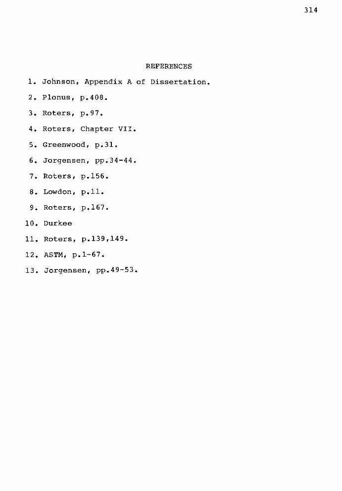
314
REFERENCES
1. Johnson, Appendix A of Dissertation.
2. Plonus, p. 408.
3. Roters, p. 97.
4. Roters, Chapter VII.
5. Greenwood, p. 31.
6. Jorgensen, pp. 34-44.
7. Roters, p. 156.
8. Lowdon, p. 11.
9. Roters, p. 167.
10. Durkee
11. Roters, p. 139, 149.
12. ASTM, p. 1-67.
13. Jorgensen, pp. 49-53.
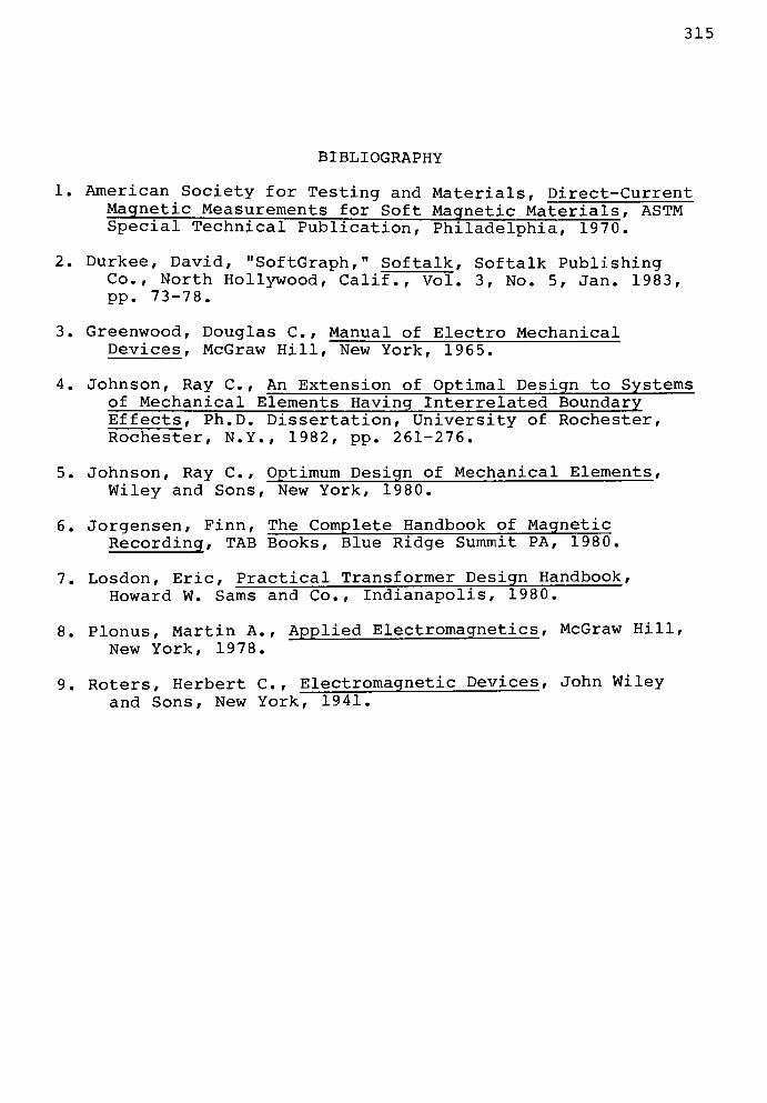
315
BIBLIOGRAPHY
1. American Society for Testing and Materials, Direct-Current
Magnetic Measurements for Soft Magnetic Materials, ASTM
Special Technical Publication, Philadelphia, 1970.
2. Durkee, David, "Sof tGraph,"
Softalk, Softalk PublishingCo., North Hollywood, Calif., Vol. 3, No. 5, Jan. 1983,
pp. 73-78.
3. Greenwood, Douglas C. , Manual of Electro Mechanical
Devices, McGraw Hill, New York, 1965.
4. Johnson, Ray C, An Extension of Optimal Design to Systems
of Mechanical Elements Having Interrelated Boundary
Effects, Ph.D. Dissertation, University of Rochester,
Rochester, N.Y. , 1982, pp. 261-276.
5. Johnson, Ray C. , Optimum Design of Mechanical Elements,
Wiley and Sons, New York, 1980.
6. Jorgensen, Finn, The Complete Handbook of Magnetic
Recording, TAB Books, Blue Ridge Summit PA, 1980.
7. Losdon, Eric, Practical Transformer Design Handbook,
Howard W. Sams and Co., Indianapolis, 1980.
8. Plonus, Martin A., Applied Electromagnetics, McGraw Hill,
New York, 1978.
9. Roters, Herbert C, Electromagnetic Devices, John Wiley
and Sons, New York, 1941.