Social Motives and Risk-Taking in InvestmentDecisions

Florian Lindner, Michael Kirchler, Stephanie Rosenkranz,UtzWeitzel

Working Papers in Economics and Statistics

2019-07

University of Innsbruckhttps://www.uibk.ac.at/eeecon/

University of InnsbruckWorking Papers in Economics and Statistics

The series is jointly edited and published by

- Department of Banking and Finance

- Department of Economics

- Department of Public Finance

- Department of Statistics

Contact address of the editor:research platform “Empirical and Experimental Economics”University of InnsbruckUniversitaetsstrasse 15A-6020 InnsbruckAustriaTel: + 43 512 507 71022Fax: + 43 512 507 2970E-mail: eeecon@uibk.ac.at

The most recent version of all working papers can be downloaded athttps://www.uibk.ac.at/eeecon/wopec/

For a list of recent papers see the backpages of this paper.

Social Motives and Risk-Taking in Investment Decisions∗

Florian Lindner, Michael Kirchler, Stephanie Rosenkranz, Utz Weitzel†

December 21, 2020

Abstract

A pervasive feature in the finance industry is relative performance, which can includeextrinsic (money), intrinsic (self-image), and reputational (status) motives. In this paper, wemodel a portfolio decision with two assets and investigate how reputational motives (i.e.,the public announcement of the winners or losers) influence risk-taking in investment deci-sions vis-a-vis intrinsic motives. We test our hypotheses experimentally with 864 studentsand 330 financial professionals. We find that reputational motives play a minor role amongfinancial professionals, as the risk-taking of underperformers is already increased due tointrinsic motives. Student behavior, however, is mainly driven by reputational motiveswith risk-taking levels that come close to those of professionals when winners or losersare announced publicly. This indicates that professionals show higher levels of intrinsic(self-image) incentives to outperform others compared to non-professionals (students), buta similar behavior can be sparked among the latter by adding reputational incentives.

JEL: D9, G2, G11, C93

Keywords: experimental finance, behavioral economics, investment game, rank incen-tives, social status, reputational motives.

∗We thank Eric Schoenberg, participants at the Experimental Finance Conference 2018 in Heidelberg, EconomicScience Association meetings 2017 in Vienna and 2018 in Berlin, the MBEES 2018 in Maastricht, seminar partici-pants in St. Gallen, Utrecht, Florence (EUI), and Obergurgl, as well as the editor and two anonymous referees forvery valuable comments. We particularly thank all financial institutions and participating professionals for the ex-cellent collaboration and their enthusiasm. Financial support from the Austrian Science Fund (FWF START-grantY617-G11 and SFB F63), Radboud University, and the Swedish Research Council (grant 2015-01713) is gratefullyacknowledged. This study was ethically approved by the IRB of the University of Innsbruck (number 15/2015).Declarations of interest: none. A prior version of the paper was circulated with the title “Social Status and Risk-Taking in Investment Decisions.”†Lindner: Max Planck Institute for Research on Collective Goods, Kurt-Schumacher-Str. 10, 53113 Bonn.

E-mail: florian.r.lindner@gmail.com. Kirchler (corresponding author): University of Innsbruck, Depart-ment of Banking and Finance, Universitätsstrasse 15, 6020 Innsbruck. Phone: +43 512 507 73014, E-mail:michael.kirchler@uibk.ac.at. Rosenkranz: Utrecht University School of Economics, Kriekenpitplein 21-22, 3584 ECUtrecht, E-mail: s.rosenkranz@uu.nl. Weitzel: Radboud University, Institute for Management Research, Heyen-daalseweg 141, 6525 AJ Nijmegen, and Vrije Universiteit Amsterdam, De Boelelaan 1105, 1081HV, Amsterdam.E-mail: u.weitzel@vu.nl.

1

1 Introduction

Recent research identified tournament incentives as an important driver for excessive risk-taking in finance (Rajan, 2006; Diamond and Rajan, 2009; Bebchuk and Spamann, 2010). In par-ticular, tournament incentives can be characterized by three major components. The first andmost obvious component is the extrinsic incentive of money, which often depends on relativeperformance. Bonuses, for example, which are widespread in the finance industry (Goetzmannet al., 2003), represent extrinsic monetary incentives for outperforming others. The second andthird components can be subsumed under rank incentives and address the intrinsic motivesof positive self-image (Bénabou and Tirole, 2006; Köszegi, 2006) and reputational motives ofimproved public status among peers (Frank, 1985; Moldovanu et al., 2007). Rank incentives re-flect an evolutionary established pattern to do better than peers and promise a non-monetaryutility to those at the top and a disutility to those at the bottom (Barankay, 2015). In line withthis, recent experimental evidence shows that rank incentives can indeed increase individuals’effort and performance (Azmat and Iriberri, 2010; Blanes-i-Vidal and Nossol, 2011; Tran andZeckhauser, 2012; Bandiera et al., 2013; Delfgaauw et al., 2013; Charness et al., 2014; Barankay,2015). Moreover, in asset market experiments with students, Schoenberg and Haruvy (2012)display either the portfolio value of the best or the worst performer to all traders and reporteffects on market prices and individual satisfaction levels.

In the finance industry, performance is very transparent, which makes it relatively easyto establish rankings and to award those that are at the top, both monetarily and with sta-tus. Annual awards to top performing fund managers, bankers, and analysts as well as theregular publication of fund rankings (e.g., Morningstar ranking) document a strong cultureof social competition.1 Given the relevance of rankings in the finance industry, as well as agrowing research on preferences for social status (see, e.g., Heffetz and Frank (2011) for anexcellent overview), there is surprisingly little literature on how social comparison impactsrisk-taking in financial decisions. The first insights into professionals’ preferences for highrank have recently been provided by Kirchler et al. (2018). In lab and online experiments, theauthors report that underperforming financial professionals increase risk-taking when facedwith non-incentivized, anonymous rankings. In the same setting, the authors find no rank-driven behavior among students. Importantly, as the rankings were anonymous and private,the authors focused on intrinsic (self-image) motives of social competition.

In this paper, we extend the insights of Kirchler et al. (2018) on rank incentives by separat-ing the effects of intrinsic (self-image) motives and reputational (status) motives on risk-taking.By disentangling these two motives we follow a similar approach as Schram et al. (2019), whoseparate the effect of social status (resulting from the social ranking of performances) from pure

1See, e.g., http://www.fmya.com/; http://www.investmentawards.com;http://www.americanbanker.com/best-in-banking/; http://excellence.thomsonreuters.com/award/starmine.

2

rivalry for resources in a real effort task. We develop a stylized theoretical model and then testthe predictions with laboratory experiments. In the model, we analyze a portfolio decisionwith two assets and investigate how reputational and intrinsic motives for being at the topor the bottom of a peer ranking influence risk-taking. We conjecture that risk-taking is higherwhen investors are informed about their rank and when top-ranked or bottom-ranked per-formers are publicly known. Moreover, our model suggests that when investors at the top orbottom of the ranking are publicly known, the risk-taking of highly ranked investors should belower than that of underperformers. To test the theoretical predictions we use the experimentaldesign of Kirchler et al. (2018) and analyze the reputational motive by announcing the winneror the loser of a group of six investors publicly at the end of the experiment. This is publicknowledge from the start of the experiment. We compare this treatment with a setting whereonly intrinsic motives can play a role, by displaying anonymous rankings privately and with-out any public announcement. This comparison is complemented with baseline treatmentswithout any rankings and, consequently, also without any public announcements. Finally, toobtain a comprehensive picture, we test our hypotheses both with 864 non-professional sub-jects (students) and with 330 financial professionals from investment-related areas (e.g., fundmanagement, trading, private banking, and asset management).2

Our results show that, first, average risk-taking among students is higher in treatments inwhich the winner or the loser is announced publicly (treatments B-WINNER and B-LOSER),compared to the baseline treatment (Treatment BASELINE). Second, we show that the publicannouncement of the winner or loser (treatments R-WINNER and R-LOSER) increases aver-age risk-taking among students compared to a treatment with anonymous rank information(Treatment RANKING). For professionals, however, we do not observe such effects. This indi-cates that reputational motives can play a role as an additional incentive, but primarily amongnon-professionals and less so among professionals. Finally, we observe that underperforminginvestors take more risk than outperformers in treatments where rankings are displayed andthe winner or loser is publicly announced (treatments R-WINNER and R-LOSER). This re-sult holds for both students and professionals. However, while underperforming students donot increase risk-taking without reputation motives, underperforming professionals increaserisk-taking primarily due to intrinsic motives and are less concerned about reputation motives(Treatment RANKING). Given professionals’ industry experience, reputational motives canbe (partly) internalized, which may explain why professionals react relatively strongly basedon intrinsic motives.

Kirchler et al. (2018) have shown that intrinsic motivation through anonymous ranking pro-motes rank-driven risk-taking among underperforming professionals but not among students.

2The experimental data of the baseline and ranking treatments are directly taken from Kirchler et al. (2018) forboth students and professionals. This study adds the public announcement of winners and losers to isolate statuseffects.

3

Our study implies that reputational motives can spark rank-driven behavior even among non-professionals, leading to substantially increased risk-taking among underperforming students.This indicates that when the full scope of motives of social comparison is addressed, i.e., in-trinsic self-image concerns as well as reputational status concerns, laypeople react similarly torankings in investment decisions as professionals do.

The remainder of the paper is organized as follows. In Section 2, we present a simplemodel of portfolio choice that incorporates non-monetary incentives and allows us to derivehypotheses for our experiment. In Section 3 we introduce the experimental design and imple-mentation. In Section 4 we present the results of the experiment. In Section 5 we discuss ourresults and conclude the paper.

2 Theoretical Framework

In the following we present a simple, stylized model that helps us to derive predictions re-garding the effects of intrinsic self-image concerns as well as reputational status concerns onrisk-taking.3 We consider a group of n investors. Every investor i ∈ n takes a portfolio deci-sion with two assets. Let us denote the expected and actual return of a risk-free asset as R f

and the expected return of a risky asset as Rm, with Rm > R f . The expected return of theinvestor i’s portfolio, Rp

i , is a weighted average of the expected return on the two assets, i.e.,Rp

i (b) = biRm + (1− bi)R f , where bi is the share of risky assets in the portfolio. Note that thestandard deviation from the portfolio σp = biσ

m.Suppose that an investor i’s utility from her portfolio’s return Ui(·) is a function of her

valuation for money νyi (derived from the portfolio return Rp

i ), her valuation νri for achieving

a certain rank ri(Rp) given the vector of portfolio returns Rp of all n investors, which stemsfrom the self-image and possibly her social image (status). Our specification of the image val-uation is inspired by Bénabou and Tirole (2006): each investor i’s preference type νi ≡ (νr

i , νyi )

is private information, only known to the investor when she invests and not observable byothers. The investor i’s image valuation depends on observers’ posterior belief regarding theinvestor i’s type νi, given her rank. In a setting with n investors, an investor i’s portfolio returnRp

i is ranked at a given rank with probability G(·, b) ≥ 0, where b = (b1, ..., bn) refers to thechoices of all n investors and · here indicates other exogenous factors (such as e.g. differencesin investors’ initial portfolio returns) that may be of influence. If the rank is observed, othersget a strong signal regarding an investor i’s type νi. The factor xk > 0 with k = r, s measuresthe visibility or salience of the rank, and its value thus depends on whether the rank will beobserved by the investor herself (xr) and others respectively (xs), where xk ∈ {0, 1}, dependingon the treatment. We assume that all investors i ∈ n simultaneously choose the share of risky

3As our aim is to predict treatment effects rather than estimates for the strength or size of underlying parame-ters, we do not present a more complex structural model that includes non-observable parameters.

4

assets bi to maximize their utility, which is given as:

Ui(Rpi (bi), bi, ri(Rp)) = ν

yi (Rp

i (bi), bi) + G(·, b)(xr + xs)νri (ri(Rp))∀i ∈ n. (1)

To keep our stylized model as tractable and intuitive as possible we make a number of sim-plifying assumptions. We assume (i) that function ν

yi (·) is twice differentiable, increasing, and

strictly concave in Rpi , while the investor i’s attitude toward risk is captured by the properties

of νyi (·) with respect to changes in bi. (ii) We consider the portfolio decision in each period t in-

dependently.4 While the function νri (·) is a discrete function in rank for ri ∈ [1, n], which itself

is a discrete increasing function of Rpi , we assume (iii) that both are also twice differentiable,

increasing, and strictly concave in their arguments. To avoid introducing further parameters,we (iv) assume that the effects of self-image and social image on utility are governed by thesame function.

Each investor i’s optimization problem can thus be written as:

maxbi(Ui(Rpi (bi), bi, ri(Rp))). (2)

Taking the derivative and rearranging the first order condition such that the marginal utilityfrom the investor i’s valuation for money ν

yi derived from the portfolio return Rp

i is on theright-hand side and her marginal image benefits νr

i for achieving a certain rank ri(Rp) are onthe left-hand side, the equilibrium portfolio, b∗i , satisfies the following first-order condition:

α

(G(·, b)

∂νri (ri(Rp))

∂ri

n

∑j=1

∂ri(Rpi (bi)))

∂Rpj

∂Rpj (bi)

∂bi+ g(·)νr

i (·))= −

(∂ν

yi (Rp

i , bi)

∂Rpi

∂Rpi (bi)

∂bi+

∂νyi (Rp

i , bi)

∂bi

),

(3)with α = (xr + xs) and g(·) denoting the derivative of G(·, b).5 In the following we willanalyse the investor’s optimal decision for the different treatments, in which either the rank isnot visible (no image valuation), is visible only to the investor (self-image), the highest (lowest)ranked investor is publicly announced (social image/status), and the combination of the lasttwo.

If investor i’s rank is not visible to herself or to others, i.e., xr = xs = 0⇒ α = 0, investor i’sdecision is non strategic and the above first-order condition resembles the textbook case whereonly the investor’s attitude toward risk will determine whether she will buy stocks on themargin or not. For a risk-neutral or risk-seeking investor, characterized by ∂ν

yi (Rp

i , bi)/∂bi ≥ 0,the right-hand side of (3) will be zero or negative, given the concavity of ν

yi (·) in Rp

i . Thus,investor i’s utility increases with a larger Rp

i , which leads to a corner solution and therefore the

4For notational convenience, we thus do not index all variables with t.5In order to focus on the basic mechanisms we assume for simplicity that the conditions for the existence of a

pure-strategy equilibria are assured.

5

optimal b̃∗ = bmax, where b̃∗ refers to investor i’s optimal choice if xr = xs = 0. In the following,we focus on the more relevant case where the investor is risk averse, i.e., ∂ν

yi (Rp

i , bi)/∂bi < 0,such that the right-hand side of (3) can be positive, and an inner solution to condition (3) exists.

Now suppose that the (risk averse) investor’s rank is visible to herself, i.e., xr > 0⇒ α > 0.As all factors on the left-hand side of (3) are positive given our concavity assumption (iii),investor i’s marginal benefits from risk taking are higher than in the absence of any intrinsicimage valuation, which induces the investor to take more risk in equilibrium, i.e. b∗i > b̃∗.

Next, , suppose that the highest (lowest) ranked investor is publicly announced such thatinvestor i’s rank is visible to others (and herself) if and only if she is the highest (lowest) rank-ing investor, i.e., xs > 0⇒ α > 0. Now status concerns will affect investors’ optimal portfoliodecisions in equilibrium. As indicated by Bénabou and Tirole (2006), it follows from (3) thatobserving an investor to be either a winner or a loser reveals the sum of her three motivations(at the margin): intrinsic, extrinsic, and reputational. Analogously to the previous case, if aninvestor’s rank is revealed to others marginal benefits from risk taking are higher than in ab-sence of any reputational / social status valuation and thus optimal risk-taking increases, i.e.b∗∗i > b̃∗.

Finally, suppose investor i’s rank is visible to the investor herself and additionally the in-vestor with the lowest (highest) rank is publicly announced. The above mentioned positivemarginal benefit for achieving a certain rank ri(Rp) is now multiplied by α = xr + xs and thusb∗∗∗i > b̃∗.

We can summarize these insights as follows:

Proposition 1 Suppose the investor is risk averse, i.e., ∂νyi (Rp

i , bi)/∂b < 0, and intrinsically values ahigher rank and status. (i) If investor i’s rank is visible to the investor herself, i.e., xr > 0, investor i’soptimal portfolio is characterized by a larger share of the risky asset than when the rank is not visible,i.e., b∗i > b̃∗. (ii) If the investor with the lowest (highest) rank is publicly announced, i.e., xs > 0,investor i’s optimal portfolio is characterized by a larger share of the risky asset than in the absence ofthe public announcement, i.e., b∗∗i > b̃∗. (iii) If investor i’s rank is visible to the investor herself andthe investor with the lowest (highest) rank is publicly announced, i.e., xr > 0 and xs > 0, investor i’soptimal portfolio is characterized by a larger share of the risky asset than when the rank is not visibleand not publicly announced, i.e., b∗∗∗i > b̃∗.

Note that investors’ extrinsic and reputational motives work in the same direction andincrease their marginal utility of taking risk. Whether the announcement of the winner or theannouncement of the loser leads investors to hold a larger share of risky assets depends on therelative strength of the extrinsic and reputational motives and can only be determined withstronger assumptions.6

6Moreover, note that although we do not indicate it explicitly in our notation, when the winner is announced,risk-taking is influenced by the probability to reach the highest rank, while when the loser is announced, risk-

6

So far we have for simplicity considered a symmetric setting. Deriving insights regardingthe choice of risk depending on an investor’s rank in a previous round is less straightforwardand closely relates to the literature on rank order tournaments with heterogeneous agents.7

Expression G(·, b) denotes the probability that, given b = (b1, ..., bn), investor i’s portfolioreturn is ranked at a certain rank. Let us for simplicity consider a situation with only twoinvestors. Then, the probability that a given investor i’s portfolio return ranks highest will be1/2 if investors are identical, for example, at the first investment decision. However, if investori’s initial return is higher at the moment of the investment decision (at later stages), then theprobability that she is ranked highest will increase in the difference between her own and theother investor’s initial portfolio return. Gürtler and Kräkel (2010) show for an analogous casethat g(·) is symmetric for both investors.8 From their analysis we can also conclude that for aninvestor with larger initial portfolio returns, G(·, b) is increasing in the initial difference. If werearrange (3), the following equation shows the effect of an investor’s initial portfolio return(expressed in a larger G(·, b) due to her rank in the previous period) on her optimal level ofrisk-taking:

α

(∂νr

i (ri(Rp))

∂ri

n

∑j=1

∂ri(Rpi (bi)))

∂Rpj

∂Rpj (bi)

∂bi

)+

g(·)G(·, b)

ανri = −

1G(·, b)

(∂ν

yi (Rp

i , bi)

∂Rpi

∂Rpi (bi)

∂bi+

∂νyi (Rp

i , bi)

∂bi

).

(4)With larger G(·, b), both sides of the equation decline. However, if α is sufficiently large, dueto the assumed concavity of νr

i , the first term in the bracket on the left-hand side is smaller foran investor with a high initial rank. Moreover, due to the asymmetric effect on all investors’ranks also the term after the summation is smaller for an investor with higher initial rank. Thisimplies that for investors with larger initial portfolio returns, the marginal reputational benefitsfrom achieving a certain rank are smaller. Hence, when the rank is visible to the investorsthemselves, underperformers take more risk than overperformers, as shown in experimentsby Kirchler et al. (2018).

In line with these arguments, we thus additionally formulate the following proposition:9

taking is influenced by the probability to reach any rank that is not the lowest. At the same time, the observers’posterior expectations of investor i’s type νi, given the announcement that the investor is not the loser, is lowerthan when the investor is announced to be the winner. In general, no clear predictions can be derived from theseconsiderations without stronger assumptions.

7See Nieken and Sliwka (2010); Gürtler and Kräkel (2010); Akerlof and Holden (2012); Balafoutas et al. (2017)for tournaments with heterogeneous agents.

8Nieken and Sliwka (2010) show for the simplified case of an asymmetric tournament with discrete choice andtwo agents that a leading player chooses the safe strategy while the lagging player chooses a risky strategy if thedifference in the outcome of some prior stage in the competition is sufficiently large and the expected returns arenot too different.

9Note that in our model all contestants are assumed to have equal types regarding their risk preferences, i.e.,all investors are identically risk averse. For Proposition 2 we, however, assume that they are heterogeneous withregard to initial portfolio returns. In this case the concavity of the utility function leads to the result that investorswith low initial portfolio returns will take more risk in equilibrium than their counterparts with high initial portfo-lio returns. This is distinct to the case of investors differing with respect to their risk attitudes and thus self-selecting

7

Proposition 2 Suppose the investor is risk averse, i.e., ∂νyi (Rp

i , bi)/∂bi < 0 and intrinsically values ahigher rank and status. If the rank is visible to the investor herself, i.e., xR > 0, low ranked investors(underperformers) are holding a larger share of risky assets than highly ranked investors. This is also thecase if additionally the rank is visible to others if and only if she is the (highest) lowest ranking investor,i.e., xS > 0.

3 Experimental Design and Hypotheses

3.1 Design and Treatments

The subjects played an investment game, which is identical to the design of Kirchler et al.(2018). Over eight periods, the participants repeatedly made portfolio choices between a risk-free alternative and a risky asset. The investment game was inspired by, and resembles gamesof, Lohrenz et al. (2007), Ehm et al. (2014), Bradbury et al. (2015), and Huber et al. (2016). Ineach period, the risk-free asset yielded a return of R f = 0.015 (1.5%) and the risky asset paidan expected return of Rm = 0.036 (3.6%) with a standard deviation of 15.9%. The participantsreceived information about the mean and standard deviation of the return distribution but noinformation about the origin of the underlying data (except that they were part of historicalfinancial market data).10 In each period, the participants decided which fraction b, RISK, oftheir current portfolio wealth, Wp, to invest in the risky asset. Portfolio wealth is carried overfrom one period to the next. The participants were allowed to invest up to 200% of theirportfolio wealth, meaning that the amount exceeding Wp was borrowed at the risk-free rateR f .11

We randomly assigned the participants to groups of six, which remained the same for theduration of the investment game. Each group played one of the six treatments in a between-subjects design. Table 1 outlines the six treatments, based on a 2x3 design with the treatment

into the ranks.10We computed these numbers from time series data of the 6-months EURIBOR for the risk-free rate (before

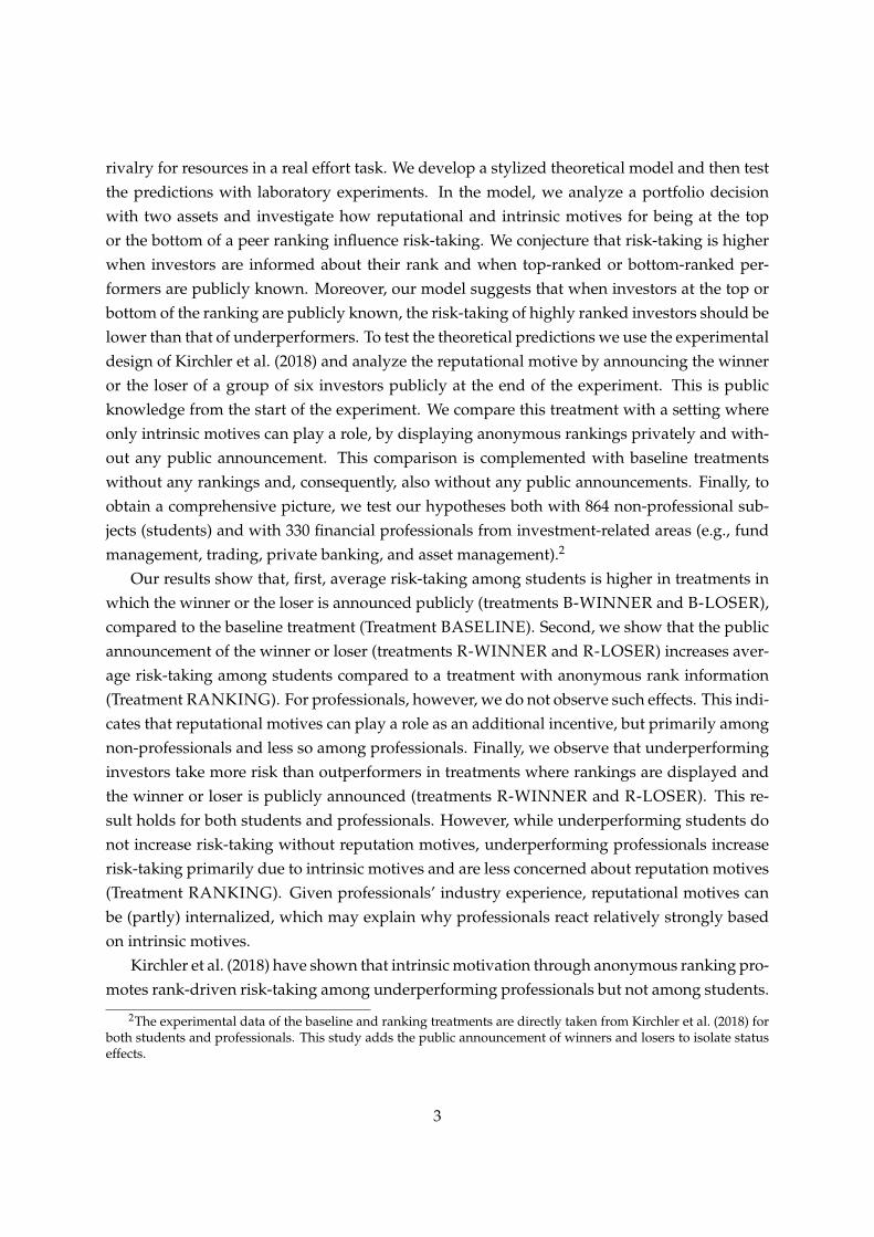
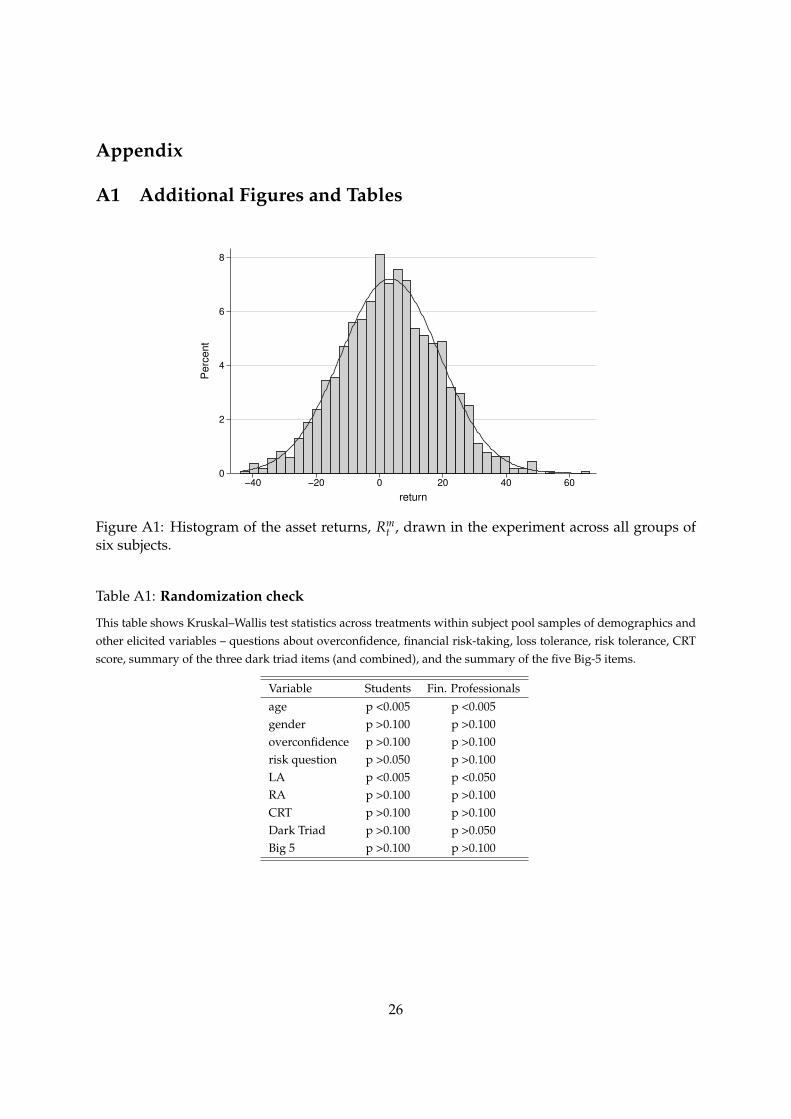
1999: FIBOR, Frankfurt Interbank Offered Rate) and from the DAX 30 for the risky asset. We calculated returnsand standard deviations for a 20-year period from January 1, 1994 to December 31, 2013. The numbers reflect semi-annual returns and standard deviations. In each period, one return was randomly drawn from a distribution withthe above mentioned two moments of the distribution. Thus, the first and second moments of the distribution werecomputed from empirical data, but the random draws in the experiment were taken from a Gaussian distributionwith same parameters. Of course, financial time series exhibit excess kurtosis and skewness, but we wanted tokeep the distribution as easily understandable as possible. Treatment RANKING served as a baseline for thereturn draws and returns drawn in this treatment were also implemented in the other treatments for the sake ofcomparability. See Figure A1 in the appendix for a histogram of the returns drawn in the experiment across allgroups of six subjects.

11Before the investment game started, the participants had to sample 30 returns from the theoretical distribu-tion with the above-mentioned first two moments of the distribution. This procedure was intended to increasefamiliarity with the properties of the risky asset. As Kaufmann et al. (2013) and Bradbury et al. (2015) report, ex-perience sampling increases decision commitment and confidence, while it can also decrease known biases such asoverestimation of loss probabilities.

8

variables “Private ranking after each period” and “Public announcement of rank after experi-ment.” The former treatment variable indicates whether an anonymous league table, detailingall group members’ current wealth levels, associated rank (RANK ∈ {1, 2, . . . , 6}), and sub-jects’ own position in the ranking, was displayed after each period. This ranking was anony-mous and not incentivized. The latter treatment variable indicates whether the top performer(Rank 1), the lowest performer (Rank 6), or nobody at all was publicly announced after thelast period.12 This procedure was common knowledge to all participants of the respective ses-sions from the beginning of the experiment (see the the instruction in the online appendix forthe exact wording). Given that the professional sample was smaller than the student sam-ple, we restricted data collection for the professionals to the four most important treatmentsto guarantee sufficient statistical power for those treatments. In particular, we did not runtreatments with professionals where only the rank after the treatment was publicly announced(“B-WINNER and B-LOSER”) .

Table 1: Treatments

This table outlines the between-subjects 2x3 treatment design. “Private ranking after each period” indicateswhether an anonymous league table, detailing all group members’ current wealth levels, associated rank(RANK ∈ {1, 2, . . . , 6}), and subjects’ own position in the ranking was displayed after each period. This rank-ing was not publicly disclosed and not incentivized. “Public announcement of rank after experiment” indicateswhether the top performer (Rank 1), the lowest performer (Rank 6), or nobody at all was publicly announcedafter the last period. Given that the professional sample was smaller than the student sample, we did not runtreatments B-WINNER and B-LOSER with professionals.

Public announcement of rank after experimentNo Yes Yes

(RANK 1) (RANK 6)Private ranking No BASELINE B-WINNER B-LOSERafter each period Yes RANKING R-WINNER R-LOSER

In Treatment BASELINE, the participants faced linear incentives and allocated their port-folio in eight periods without peer feedback. Students received an initial endowment of 30euro (90 euro for professionals) and accumulated gains and losses depending on their invest-ments over time. In line with Cohn et al. (2014, 2017) and Kirchler et al. (2018), each participantreceived the payout of the investment game with a probability of 20% to facilitate high stakes.There is a growing body of literature indicating that these commonly used payment schemeswith random components do not bias risk-taking behavior in experiments (Starmer and Sug-den, 1991; Cubitt et al., 1998; Hey and Lee, 2005; March et al., 2015). Moreover, Charness et al.

12The main reasons why we decided to only announce the top or the lowest performer are the following. First,we wanted to isolate the reputation (announcement) effect as much as possible. With only announcing the winneror the loser, we can control for confounding effects that might arise when announcing the entire ranking publicly.Second, in the related literature on rank-order tournament it is common to design tournaments with one winnerprize and N − 1 loser prizes (see e.g. Dutcher et al., 2015, among others).

9

(2016) pointed out that the pay-one (or pay-a-subset) method is either equal or even superiorto the pay-all method in the majority of cases.

The treatments B-LOSER and B-WINNER are identical to BASELINE with the only dif-ference that, respectively, the worst performer (loser) or the top performer (winner) in theranking of each group was publicly announced after the last period of the investment game.This procedure was common knowledge from the beginning of the experiment.

In Treatment RANKING, the participants received the same linear incentives as in BASELINE,but after each period we showed them an anonymous league table, detailing all group mem-bers’ current wealth levels, associated rank (RANK ∈ {1, 2, . . . , 6}), and their own positionin the ranking. This ranking was not incentivized, and there was no public disclosure of theranking in the end. Hence, we apply a very mild form of social comparison in this treatment.All data of treatments BASELINE and RANKING are taken from the experiments in Kirchleret al. (2018).13

Treatments R-LOSER and R-WINNER are identical to Treatment RANKING, except forthe announcement of the loser or the winner, respectively, according to the ranking in eachgroup. The treatments with the public announcement of the loser, or respectively the winner,are designed to investigate the effect of reputational motives beyond intrinsic rank incentives.

After the investment game, in a second part of the experiment, we administered two addi-tional experimental tasks, one of which was paid out randomly, and some survey questions.Please see the online appendix for the instructions of all experimental tasks. Part 2 of the in-structions were handed out after all participants had completed Part 1. In the first task wemeasured risk-attitudes in a standard choice list setting (Bruhin et al., 2010; Abdellaoui et al.,2011).14 We also measured risk attitudes/tolerance (on a Likert scale from 1 to 7) with a surveyquestion from the German Socio-Economic Panel (SOEP; Dohmen et al., 2011). The partici-pants answered the question: “How do you see yourself: Are you willing to take risks or tryto avoid risks?” The answers were provided on a Likert scale from 1 (not at all willing to takerisks) to 7 (very willing to take risks). In the second task, we measured loss tolerance using theprocedure of Gächter et al. (2010).15 The participants earned 18 euro as a show-up fee for par-ticipating in the experiment, which covered the potential maximum loss in the loss tolerancetask. In the survey, we measured the participants’ attitudes toward social comparison withthree questions on social status, financial success, and relative performance, taken from Cohnet al. (2014). Furthermore, we measured CRT scores (Cognitive Reflection Test, Frederick, 2005)

13In Kirchler et al. (2018) the treatments BASELINE and RANKING are referred to as TBASE and TRANK,respectively.

14The participants could choose between a risky option, paying either 0 or 8 euro with equal probability, or asafe payment, which ranged between 1 and 7 euro in steps of 1 euro.

15In the task measuring loss tolerance, the participants had to decide whether to play a particular lottery or not.If they decided to play the lottery, they either received, with equal probability, 15 euro or incured a loss of X. Theloss X varied from 1 to 6 euro in steps of 1 euro. If the participants decided not to play a particular lottery, theyreceived a payout of zero.

10

with slightly modified questions (see appendix).16 Questions on demographics concluded theexperiment.

3.2 Hypotheses

We can now use the treatments defined above to operationalize the propositions from themodel. Proposition 1 allows us to formulate hypotheses regarding portfolio choice in dif-ferent treatments in which investors are informed about their rank and/or the winner or loseris publicly announced:

Hypothesis 1 Risk-taking is higher in treatments where investors are informed about their rank (RANKING),compared to the baseline treatment (BASELINE).

Hypothesis 2 If investors are not informed about their rank, risk-taking is higher in treatments wherethe winner or the loser is announced (B-LOSER and B-WINNER), compared to the baseline treatment(BASELINE).

Hypothesis 3 In treatments where investors are informed about their rank and where the winner orthe loser is announced (R-LOSER and R-WINNER), risk-taking is higher compared to the treatmentwithout announcement (RANKING).

Moreover, based on Proposition 2, we can formulate hypotheses with respect to the portfo-lio choice of highly ranked investors in comparison to underperformers.

Hypothesis 4 In treatments where investors are informed about their rank (RANKING), the risk-taking of highly ranked investors is lower compared to risk-taking of underperformers.

Hypothesis 5 In treatments where investors are informed about their rank and where the winner orthe loser is announced (R-LOSER and R-WINNER), the risk-taking of highly ranked investors islower compared to risk-taking of underperformers.

3.3 Implementation

To test our hypotheses we recruited 864 student subjects for Experiment STUD, i.e., 144 sub-jects for each treatment. We administered the experiment to bachelor and master students

16In Table A4 in the appendix we analyze the impact of these control variables on the average level of risktaking of the individuals in the experiment. We find that loss tolerance has the highest explanatory power inexplaining risk taking in the experiment (i.e., with a highly significant positive coefficient in both subject pools). Wealso elicited the 10-item Big-5 personality traits according to Rammstedt and John (2007) and socially undesirablepersonality traits, such as narcissism, psychopathy, and machiavellianism (i.e., Dark Triad), using the 12-item testof Jonason and Webster (2010). We did not include the Big-5 and Dark Triad personality traits to Table A4, becauseof missing data points. The questions asked in the survey were programmed in a separate z-Tree file, which willbe provided upon request.

11

from various disciplines at the University of Innsbruck (Austria) at the Innsbruck EconLab.We recruited 75.7% male students to stay as close as possible to the gender ratio of the pro-fessionals in Experiment PROF (see below). The average age was 23.2 years, and 47.7% werestudents with a major in economics or management. The students received an average payoutof 17 euro for both parts of Experiment STUD with a maximum payout of 161 euro and anaverage duration of 45 minutes per session. We paid out subjects privately, in cash, after theexperiment. We programmed and conducted all experiments (STUD and PROF) using thesame source code, programmed in z-Tree (Fischbacher, 2007). Student subjects were recruitedvia hroot (Bock et al., 2014).

For Experiment PROF we recruited 330 professionals from major financial institutions inseveral OECD countries. All professionals that participated in our experiments were regu-larly confronted with competitive rankings, bonus incentives, and investment decisions—i.e.,professionals from private banking, trading, investment banking, portfolio management, fundmanagement, and wealth management.17 In Experiment PROF, 87.3% of the participants weremale, their average age was 36.8 years, and they had been working in the finance industry for12.6 years on average.

In all experiments with professionals, we booked a conference room on location or in closeproximity (for several organizations to participate simultaneously), set up our mobile labo-ratory, and invited professionals to show up. Our mobile laboratory is virtually identical tothe Innsbruck EconLab at the University of Innsbruck, where we ran the experiment with stu-dents (see pictures in the appendix). The mobile lab consists of laptops and partition wallson all sides for each participant, allowing for conditions similar to those in regular experi-mental laboratories. We mainly recruited members of professional associations/societies, en-suring that most sessions were populated with professionals from different institutions. Inthis way, we achieved high comparability with the student sample, as most professionals didnot know, or barely knew, each other. In total, 78, 102, 66, and 84 professionals participatedin treatments BASELINE, RANKING, R-LOSER, and R-WINNER, respectively. Becauseof a limited number of professionals we refrained from running treatments R-LOSER andR-WINNER in Experiment PROF and rather focused on a sufficiently large sample in thefour other treatments.18

All specifications were identical to the experiment with students except for the stake size.Similar to other studies (List and Haigh, 2005; Alevy et al., 2007; Cohn et al., 2014; Kirchler et al.,2018), we scaled up the students’ payoffs with a multiplier of three for professionals in all partsof the experiment. The professionals received an average payout of 48 euro for both parts ofExperiment PROF, with a maximum payout of 286 euro and an average duration of 45 minutesper session. For participants who received money in the investment game, the average payout

17We signed non-disclosure agreements (NDA) regarding the identity of the participating financial institutions.18More specifically, we decided to conduct the most “extreme” treatments with financial professionals.

12

was 112 euro for a task of 20 minutes, ensuring salient incentives for professionals.19 Theprofessionals received the payout in sealed envelopes and in cash directly after the experiment.

4 Results

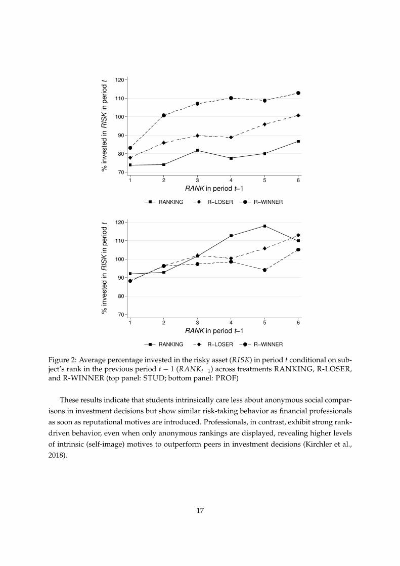
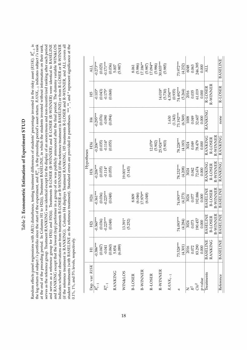
To test Hypotheses H1 to H5, we run random effects panel regressions with AR(1) distur-bance.20 In all specifications, the percentage that subjects invested in the risky asset (RISK) isthe dependent variable. As control variables, we include Rp

t−1 , which measures the log-returnof subject i’s portfolio since the start of the experiment, and Rm

t−1 , which records the precedingperiod’s asset return. With treatment dummies we test for differences between treatments, asdefined in the hypotheses. With RANKt−1, which denotes subject i’s rank at the end of thepreceding period, we analyze the effect of relative performance on risk-taking. The results arereported in Table 2 (STUD) and Table 3 (PROF). Furthermore, we run the same regression withall treatments to draw a complete picture over all treatments (with BASELINE as referencetreatment; see columns ALL).21

Result 1 (H1): Average risk-taking does not differ between treatments where investors are informedabout their rank (RANKING) and the baseline treatment (BASELINE). This holds for both experi-ments, STUD and PROF.

The coefficients of the intercept and of the treatment dummy RANKING in the first col-umn of Tables 2 and 3 show the levels of risk-taking in the two relevant treatments. Risk-takingin Experiment STUD increases from 73.5% (coefficient of α) in Treatment BASELINE to 79.4%in Treatment RANKING (sum of coefficients of α and of dummy RANKING). However, thisincrease is not statistically significant (at p = 0.336), as shown by the standard errors for thedummy RANKING. In Experiment PROF, the level of risk-taking is generally higher thanin Experiment STUD: the corresponding levels of risk-taking by professionals are 97.0% and

19In the questionnaire, the professionals reported an average annual gross salary of 76,548 euro. Accordingly,the average (maximum) hourly payoff from the experiment amounted to roughly 2.9 times (18 times) the averageprofessional’s hourly wage after taxes. For this calculation, we assumed a working time of 45 hours/week for 47weeks/year and 40% taxes to calculate an hourly net wage (22 euro). In our experiment, the participants’ average(maximum) hourly payment was 64 (381) euro (48*60/45 and 286*60/45), resulting in 295% (1,756%) of their salary.Haigh and List (2005) report that their average traders’ payment for a 25-minute task was 40 U.S. dollars, whichtranslates to an hourly payment of 96 U.S. dollars. Given an exchange rate of about 1.32 at the time of the study,the payment in Haigh and List (2005) is equivalent to an average hourly wage of 73 euro. Note that monetaryincentives in experiments with a representative sample of the general population are less accurate because of thehigh heterogeneity in the participants’ salaries. In our case, the hourly payout of nearly three times the averageapplies to a sample with a more homogeneous salary distribution.

20See Table A1 in the appendix for a randomization check. It turns out that the only variables that are signif-icantly different across treatments are age and loss tolerance. As a robustness check, we add these two controlvariables in the regression models, leading to qualitatively identical results. See Table A2 and Table A3 in theappendix for details.

21As a robustness check, we run Table 3 including the years in the finance industry as a proxy of work experi-ence. We do not detect differences to the main results, outlining that younger professionals do not exhibit differentbehavior to professionals with longer tenure in the industry. Results can be provided upon request.

13

104.4% in Treatments BASELINE and RANKING, respectively. Again, this increase is notstatistically significant. This result is in line with Kirchler et al. (2018). We include it for thesake of completeness and as a comparison for our analyses of status concerns in the followinghypotheses.

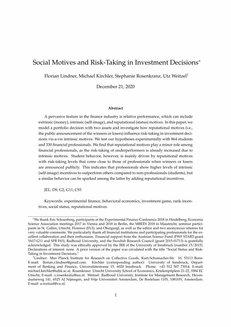
Result 2 (H2): In Experiment STUD, average risk-taking is higher in treatments in which thewinner or the loser is announced (B-WINNER and B-LOSER), compared to the baseline treatment(BASELINE).

Recall that we did not run Treatments B-WINNER and B-LOSER in Experiment PROF.We therefore test Hypothesis 2 with Experiment STUD only. As reported in Columns 2 and 3 ofTable 2, average risk-taking in treatments accounting for reputational motives is significantlyhigher compared to the baseline treatment in Experiment STUD. When pooling TreatmentsB-WINNER and B-LOSER with the dummy WIN&LOS, the effect of reputational motives onrisk-taking is significant at a 5% level. This effect is mainly driven by announcing top perform-ers in Treatment B-WINNER, with a highly significant increase of risk-taking by 18 percentagepoints (and an average level of risk-taking of 92.1%). When the bottom-ranked subjects are an-nounced in Treatment B-LOSER, average risk-taking is 82.9% and not statistically differentfrom the baseline treatment.

Result 3 (H3): In Experiment STUD, average risk-taking is higher when investors are informedabout their rank and when the winner or the loser is announced (R-WINNER and R-LOSER), com-pared to no announcement (RANKING). This effect does not hold in Experiment PROF.

As shown in Columns 4 and 5 of Table 2, even when controlling for intrinsic rank incen-tives, reputational motives in Treatments R-WINNER and R-LOSER significantly increaseaverage risk-taking compared to Treatment RANKING in Experiment STUD. This effect is,again, mainly driven by the announcement of top performers in Treatment R-WINNER, sim-ilar to the above results in support of Hypothesis 2. The aggregate effect of both treatments(dummy WIN&LOS), reported in Column 4, is significant at a 0.1% level. For professionals,we find no differences in average risk-taking between Treatments R-WINNER, R-LOSER,and RANKING (see Columns 2 and 3 of Table 3). This striking difference in behavior com-pared to the student sample may be due to the relatively high risk-taking of underperformingprofessionals in RANKING. We will return to this finding when testing Hypothesis H4.

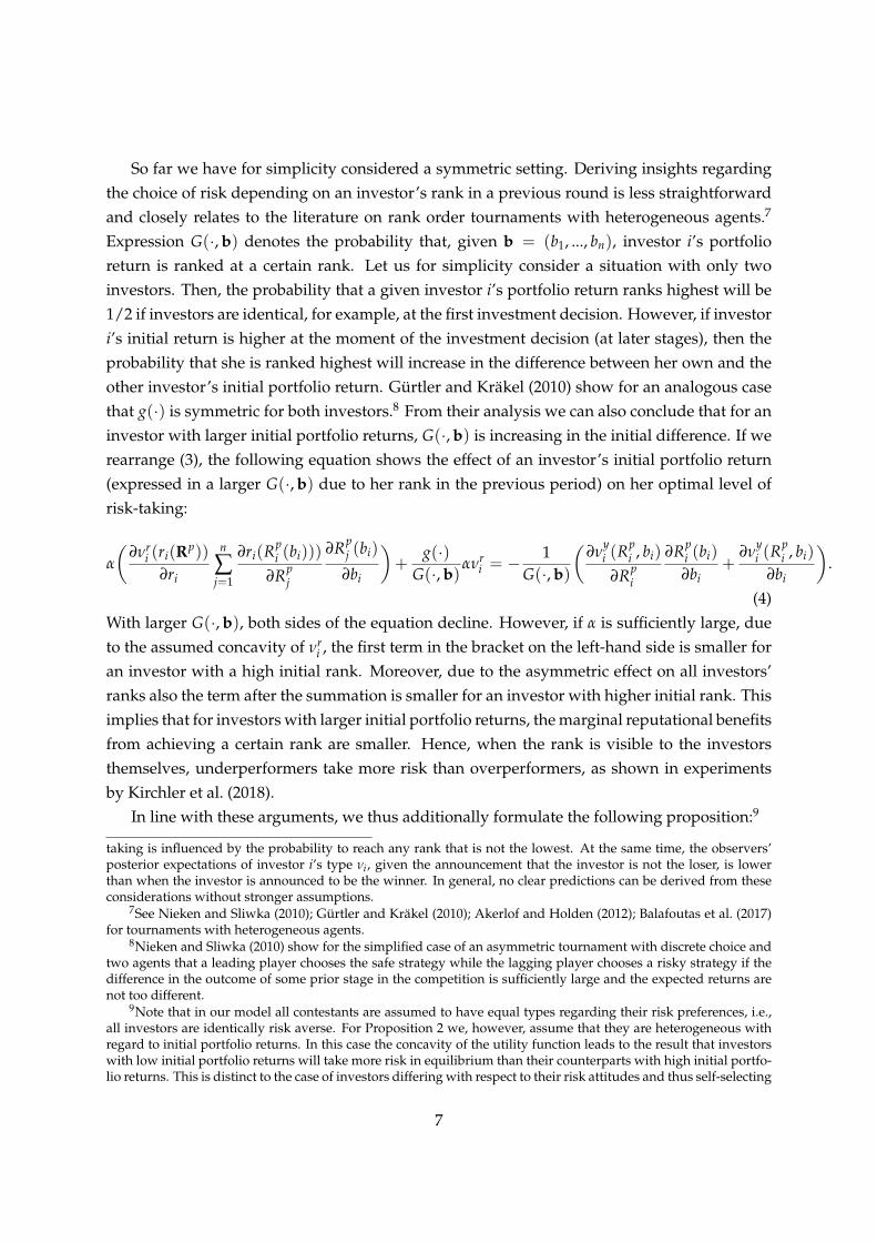
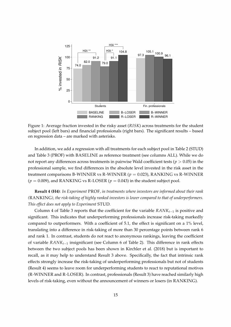
For illustrative purpose, we present the results of average risk-taking graphically in Fig-ure 1 for hypotheses H1 to H3. Note that the values are taken from the regression in column“ALL” of the respective subject pool.

14

74.082.0

91.2

79.0

91.1

104.897.3

105.1100.9

96.1

H2ii **

H3ii ***

H3ii *

0

25

50

75

100

125

% investe

d in R

ISK

Students Fin. professionals

BASELINE B−LOSER B−WINNER

RANKING R−LOSER R−WINNER

Figure 1: Average fraction invested in the risky asset (RISK) across treatments for the studentsubject pool (left bars) and financial professionals (right bars). The significant results – basedon regression data – are marked with asterisks.

In addition, we add a regression with all treatments for each subject pool in Table 2 (STUD)and Table 3 (PROF) with BASELINE as reference treatment (see columns ALL). While we donot report any differences across treatments in pairwise Wald coefficient tests (p > 0.05) in theprofessional sample, we find differences in the absolute level invested in the risk asset in thetreatment comparisons B-WINNER vs R-WINNER (p = 0.023), RANKING vs R-WINNER(p = 0.009), and RANKING vs R-LOSER (p = 0.043) in the student subject pool.

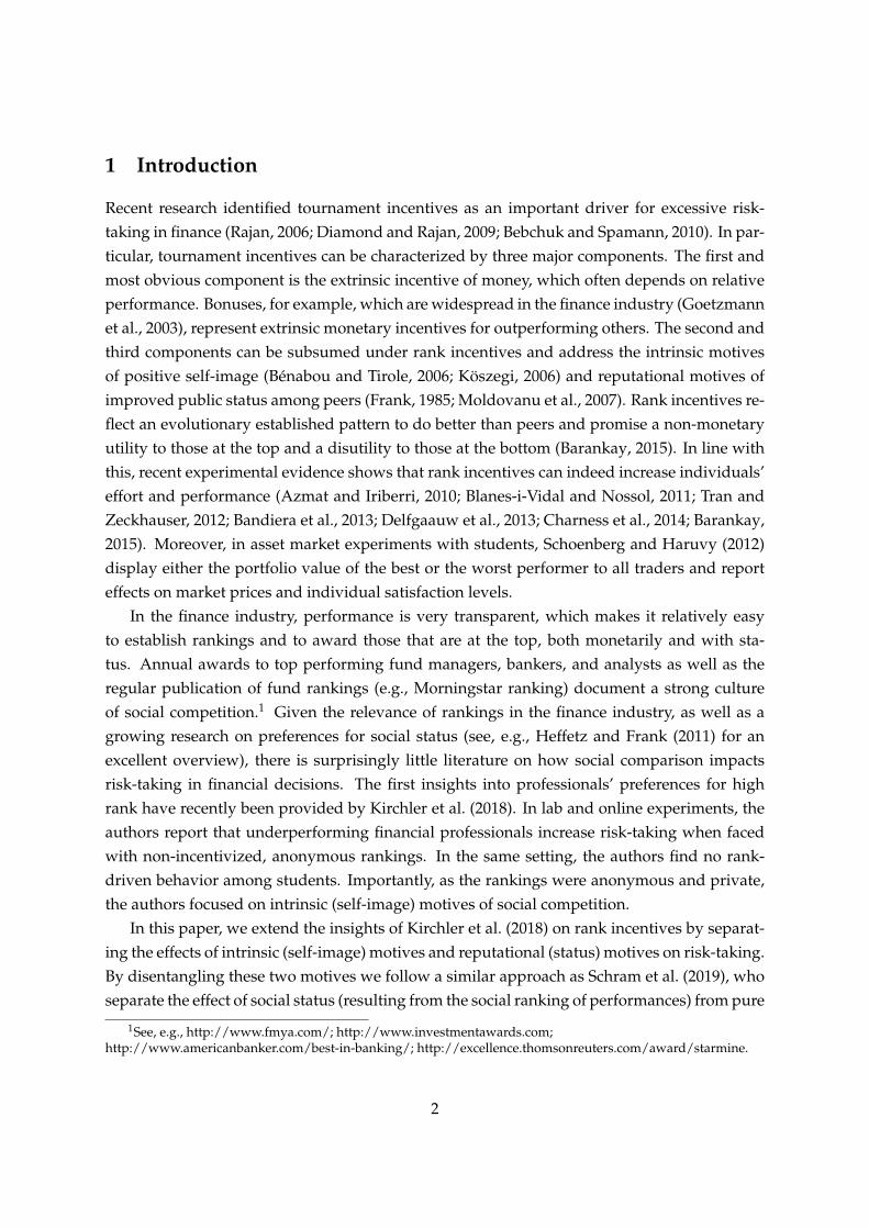
Result 4 (H4): In Experiment PROF, in treatments where investors are informed about their rank(RANKING), the risk-taking of highly ranked investors is lower compared to that of underperformers.This effect does not apply to Experiment STUD.

Column 4 of Table 3 reports that the coefficient for the variable RANKt−1 is positive andsignificant. This indicates that underperforming professionals increase risk-taking markedlycompared to outperformers. With a coefficient of 5.1, the effect is significant on a 1% level,translating into a difference in risk-taking of more than 30 percentage points between rank 6and rank 1. In contrast, students do not react to anonymous rankings, leaving the coefficientof variable RANKt−1 insignificant (see Column 6 of Table 2). This difference in rank effectsbetween the two subject pools has been shown in Kirchler et al. (2018) but is important torecall, as it may help to understand Result 3 above. Specifically, the fact that intrinsic rankeffects strongly increase the risk-taking of underperforming professionals but not of students(Result 4) seems to leave room for underperforming students to react to reputational motives(R-WINNER and R-LOSER). In contrast, professionals (Result 3) have reached similarly highlevels of risk-taking, even without the announcement of winners or losers (in RANKING).

15

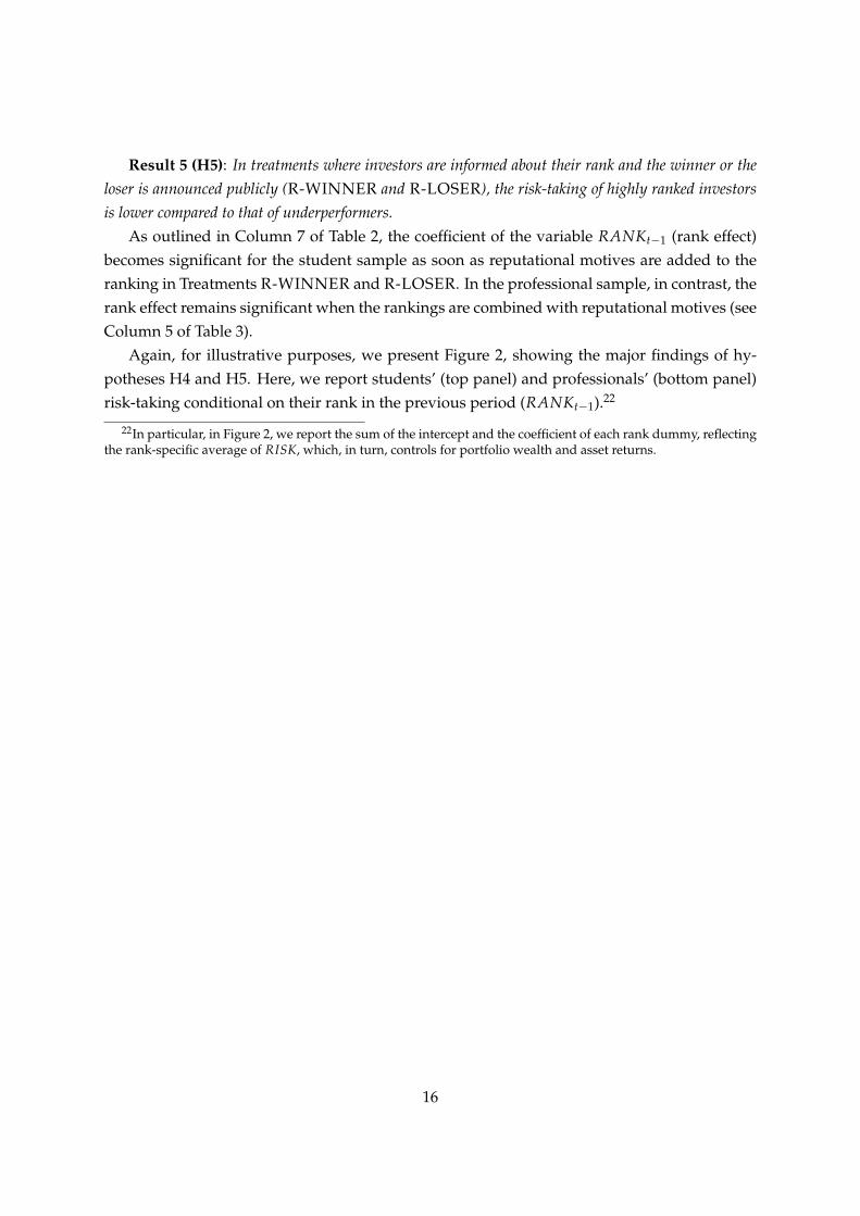
Result 5 (H5): In treatments where investors are informed about their rank and the winner or theloser is announced publicly (R-WINNER and R-LOSER), the risk-taking of highly ranked investorsis lower compared to that of underperformers.

As outlined in Column 7 of Table 2, the coefficient of the variable RANKt−1 (rank effect)becomes significant for the student sample as soon as reputational motives are added to theranking in Treatments R-WINNER and R-LOSER. In the professional sample, in contrast, therank effect remains significant when the rankings are combined with reputational motives (seeColumn 5 of Table 3).

Again, for illustrative purposes, we present Figure 2, showing the major findings of hy-potheses H4 and H5. Here, we report students’ (top panel) and professionals’ (bottom panel)risk-taking conditional on their rank in the previous period (RANKt−1).22

22In particular, in Figure 2, we report the sum of the intercept and the coefficient of each rank dummy, reflectingthe rank-specific average of RISK, which, in turn, controls for portfolio wealth and asset returns.

16

70

80

90

100

110

120

% investe

d in R

ISK

in p

eriod t

1 2 3 4 5 6

RANK in period t−1

RANKING R−LOSER R−WINNER

70

80

90

100

110

120

% investe

d in R

ISK

in p

eriod t

1 2 3 4 5 6

RANK in period t−1

RANKING R−LOSER R−WINNER

Figure 2: Average percentage invested in the risky asset (RISK) in period t conditional on sub-ject’s rank in the previous period t− 1 (RANKt−1) across treatments RANKING, R-LOSER,and R-WINNER (top panel: STUD; bottom panel: PROF)

These results indicate that students intrinsically care less about anonymous social compar-isons in investment decisions but show similar risk-taking behavior as financial professionalsas soon as reputational motives are introduced. Professionals, in contrast, exhibit strong rank-driven behavior, even when only anonymous rankings are displayed, revealing higher levelsof intrinsic (self-image) motives to outperform peers in investment decisions (Kirchler et al.,2018).

17

Tabl

e2:

Econ

omet

ric

Esti

mat

ion

ofEx

peri

men

tST

UD

Ran

dom

effe

cts

pane

lreg

ress

ions

wit

hA

R(1

)di

stur

banc

e,te

stin

gtr

eatm

entd

iffer

ence

sof

stud

ents

’per

cent

age

inve

sted

inth

eri

sky

asse

t(R

ISK

).R

p t−1

isth

elo

g-re

turn

ofsu

bjec

ti’s

port

folio

sinc

eth

est

arto

fth

eex

peri

men

t,an

dR

m t−1

isth

epr

eced

ing

peri

od’s

asse

tret

urn.

RA

NK

t−1

indi

cate

ssu

bjec

ti’s

rank

atth

een

dof

the

prec

edin

gpe

riod

.In

Col

umns

H1

toH

2(ii)

,Tre

atm

ent

BA

SEL

INE

,in

whi

chth

est

uden

tsin

vest

edw

itho

utin

form

atio

non

thei

rra

nk,

serv

esas

the

refe

renc

egr

oup.

Trea

tmen

tRA

NK

ING

was

iden

tica

lexc

eptf

orth

edi

spla

yof

anan

onym

ous

and

non-

ince

ntiv

ized

rank

ing

afte

rea

chpe

riod

and

serv

esas

are

fere

nce

grou

pfo

rH

3(i)

and

H3(

ii).

Trea

tmen

tsB

-LO

SER

(B-W

INN

ER

)an

dR

-LO

SER

(R-W

INN

ER

)w

ere

iden

tica

lto

BA

SEL

INE

and

RA

NK

ING

exce

ptth

atth

elo

wes

t(t

op)

perf

orm

erin

agr

oup

ofsi

xw

aspu

blic

lyan

noun

ced

afte

rth

efin

alpe

riod

.Th

edu

mm

yva

riab

leW

IN&

LO

Sin

dica

tes

whe

ther

obse

rvat

ions

are

from

trea

tmen

tsB

-LO

SER

orB

-WIN

NE

R(i

fthe

refe

renc

etr

eatm

enti

sB

ASE

LIN

E)o

rfr

omR

-LO

SER

orR

-WIN

NE

R(i

fth

ere

fere

nce

trea

tmen

tis

RA

NK

ING

).C

olum

nH

4di

spla

ysTr

eatm

ent

RA

NK

ING

,H5

trea

tmen

tsR

-LO

SER

and

R-W

INN

ER

,and

ALL

cove

rsal

lst

uden

ttr

eatm

ents

(wit

hB

ASE

LIN

Eas

the

refe

renc

etr

eatm

ent)

.St

anda

rder

rors

are

prov

ided

inpa

rent

hese

s.**

*,**

,and

*re

pres

ent

sign

ifica

nce

atth

e0.

1%,1

%,a

nd5%

leve

ls,r

espe

ctiv

ely.

Hyp

othe

ses

Dep

.var

:RIS

KH

1H

2iH

2ii

H3i

H3i

iH

4H

5A

LLR

p t−1

-0.3

86**

*-0

.360

***

-0.3

61**

*-0

.206

***

-0.2

06**

*-0

.295

***

-0.1

03*

-0.2

73**

*(0

.047

)(0

.036

)(0

.036

)(0

.035

)(0

.035

)(0

.076

)(0

.043

)(0

.025

)R

m t−1

-0.0

41-0

.225

***

-0.2

25**

*-0

.114

*-0

.114

*-0

.090

-0.1

75*

-0.1

71**

*(0

.060

)(0

.048

)(0

.048

)(0

.055

)(0

.055

)(0

.094

)(0

.068

)(0

.036

)R

AN

KIN

G5.

854

5.00

7(6

.089

)(5

.987

)W

IN&

LO

S13

.391

*19

.001

***

(5.2

52)

(5.1

43)

B-L

OSE

R8.

809

8.06

1(6

.046

)(5

.986

)B

-WIN

NE

R17

.979

**17

.186

**(6

.048

)(5

.987

)R

-LO

SER

12.0

79*

17.0

94**

(5.9

02)

(5.9

86)

R-W

INN

ER

25.9

24**

*14

.018

*30

.835

***

(5.9

03)

(5.7

30)

(5.9

85)

RA

NK

t−1

1.63

04.

354*

**(1

.343

)(0

.935

)α

73.5

28**

*74

.093

***

74.0

93**

*78

.232

***

78.2

28**

*73

.192

***

74.4

92**

*73

.972

***

(4.3

01)

(4.2

84)

(4.2

73)

(4.2

08)

(4.1

83)

(6.5

69)

(5.2

64)

(4.2

32)

N20

1630

2430

2430

2430

2410

0820

1660

48R

20.

072

0.07

30.

077

0.04

20.

049

0.04

90.

035

0.06

3C

hi2

83.2

9019

0.45

719

2.88

672

.674

78.4

7932

.607

61.0

1924

6.39

5p-

valu

e0.

000

0.00

00.

000

0.00

00.

000

0.00

00.

000

0.00

0Tr

eatm

ents

BA

SEL

INE

BA

SEL

INE

BA

SEL

INE

RA

NK

ING

RA

NK

ING

RA

NK

ING

R-L

OSE

RA

LLR

AN

KIN

GB

-LO

SER

B-L

OSE

RR

-LO

SER

R-L

OSE

RR

-WIN

NE

RB

-WIN

NE

RB

-WIN

NE

RR

-WIN

NE

RR

-WIN

NE

RR

efer

ence

BA

SEL

INE

BA

SEL

INE

BA

SEL

INE

RA

NK

ING

RA

NK

ING

none

R-L

OSE

RB

ASE

LIN

E

18

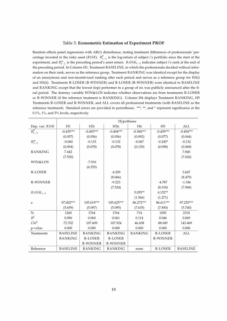
Table 3: Econometric Estimation of Experiment PROF

Random effects panel regressions with AR(1) disturbance, testing treatment differences of professionals’ per-centage invested in the risky asset (RISK). Rp

t−1 is the log-return of subject i’s portfolio since the start of theexperiment, and Rm

t−1 is the preceding period’s asset return. RANKt−1 indicates subject i’s rank at the end ofthe preceding period. In Column H1, Treatment BASELINE, in which the professionals decided without infor-mation on their rank, serves as the reference group. Treatment RANKING was identical except for the displayof an anonymous and non-incentivized ranking after each period and serves as a reference group for H3(i)and H3(ii). Treatments B-LOSER (B-WINNER) and R-LOSER (R-WINNER) were identical to BASELINEand RANKING except that the lowest (top) performer in a group of six was publicly announced after the fi-nal period. The dummy variable WIN&LOS indicates whether observations are from treatments R-LOSERor R-WINNER (if the reference treatment is RANKING). Column H4 displays Treatment RANKING, H5Treatments R-LOSER and R-WINNER, and ALL covers all professional treatments (with BASELINE as thereference treatment). Standard errors are provided in parentheses. ***, **, and * represent significance at the0.1%, 1%, and 5% levels, respectively.

HypothesesDep. var: RISK H1 H3i H3ii H4 H5 ALLRp

t−1 -0.435*** -0.493*** -0.494*** -0.384*** -0.439*** -0.454***(0.057) (0.056) (0.056) (0.092) (0.077) (0.044)

Rmt−1 -0.060 -0.133 -0.132 -0.067 -0.245* -0.132

(0.094) (0.078) (0.078) (0.129) (0.098) (0.068)RANKING 7.442 7.840

(7.520) (7.626)WIN&LOS -7.016

(6.555)R-LOSER -4.209 3.647

(8.066) (8.479)R-WINNER -9.223 -4.787 -1.186

(7.524) (8.318) (7.968)RANKt−1 5.055** 4.152**

(1.566) (1.271)α 97.002*** 105.619*** 105.625*** 86.272*** 86.611*** 97.253***

(5.659) (5.097) (5.095) (7.635) (7.850) (5.740)N 1260 1764 1764 714 1050 2310R2 0.096 0.060 0.061 0.114 0.046 0.069Chi2 72.702 107.609 107.924 46.438 88.045 143.469p-value 0.000 0.000 0.000 0.000 0.000 0.000Treatments BASELINE RANKING RANKING RANKING R-LOSER ALL

RANKING R-LOSER R-LOSER R-WINNERR-WINNER R-WINNER

Reference BASELINE RANKING RANKING none R-LOSER BASELINE

19

5 Conclusion

In this paper, we presented theoretical mechanisms and experimental evidence regarding howrank incentives impact risk-taking in investment decisions among 864 non-professionals (stu-dents) and 330 financial professionals from investment-related areas, such as fund manage-ment, trading, private banking, and asset management. In particular, we separate intrinsic(self-image) and reputational (status) motives and investigate their contribution to risk-takingin investment decisions.

We found that average risk-taking among students is higher in treatments in which thewinner or the loser is announced publicly, compared to the baseline treatment. The public an-nouncement of winners or losers also increases average risk-taking among students comparedto a treatment with anonymous rank information. For professionals, however, we do not ob-serve such effects, which indicates that reputation motives primarily play a role among non-professionals. We also find that underperforming investors take more risk than outperformersin treatments where both intrinsic and reputational motives are possible drivers, i.e., whererankings are displayed and the winner or loser is publicly announced. This result holds forboth students and professionals. However, while underperforming students do not increaserisk-taking without reputational motives, underperforming professionals increase risk-takingprimarily in treatments where intrinsic motives play a role. Hence, reputational motives, asan additional incentive, seem to be of less importance for financial professionals, as the rank-driven behavior of underperformers is already strong when anonymous rankings are in place.This could cautiously be interpreted as professionals showing higher levels of intrinsic (self-image) motives to outperform others compared to non-professionals (students) in investmentdecisions.

Our results differ compared to the findings of Gilpatric (2009) in a tournament setting.The main reason is that the authors, in contrast to our approach, focus on symmetric equilib-ria and assume risk neutral, identical contestants. Their main conclusion is that risk takingcan be mitigated or eliminated by structuring the contest with more than two payoff levels,specifically by introducing a fine for the contestant ranking last. Another reason why our re-sults differ from previous findings in contest settings, specifically rank-order tournaments, isthat agents in tournaments usually earn either one high prize or one of n-1 low prizes (seeDechenaux et al., 2015, for a comprehensive survey). In our experiment, however, each sub-ject receives a payment that solely depends on his/her final portfolio value. This paymentis determined by individual risk-taking and is completely independent of others’ choices. Inmonetary terms this implies a different strategic situation than in tournament settings. In tour-naments, subjects, who are behind, or belief that the likelihood of winning is low, might giveup and maximize their own profit in minimizing the effort costs. The result is a U-shaped ef-fort distribution: some people try to win and invest a lot of effort and others will invest very

20

little or almost no effort (Dutcher et al., 2015).Our results also have welfare implications. If professionals care about their ranking vis-

a-vis their peers, we show that they will increase risk-taking. As professionals mostly do notinvest their own money, this behavior may exceed the risk bearing capacity of their clients,which can lead to a situation where professionals take excessive risks with their customers’money because of their private social motives. If that is the case, regulators should considerputting restrictions on providing rank information in financial markets. Note that regulatorsshould focus on private rank information as we find that reputation does not seem to addmuch risk-taking.

Of course, this paper can only attempt to shed some light on the complex relationshipsbetween extrinsic, intrinsic, and reputational motives on risk-taking and the possible importof professional norms and values into competitive investment decisions. Further research isneeded to disentangle these mechanisms and their effects on risk-taking and decision-makingin general.

21

References

Abdellaoui, Mohammed, Aurélien Baillon, Laetitia Placido, Peter P. Wakker. 2011. The richdomain of uncertainty: Source functions and their experimental implementation. AmericanEconomic Review 101(2) 695–723.

Akerlof, Robert J., Richard T. Holden. 2012. The nature of tournaments. Economic Theory 51(2)289–313.

Alevy, Jonathan E., Michael S. Haigh, John A. List. 2007. Information cascades: Evidence froma field experiment with financial market professionals. Journal of Finance 62(1) 151–180.

Azmat, Ghazala, Nagore Iriberri. 2010. The importance of relative performance feedback in-formation: Evidence from a natural experiment using high school students. Journal of PublicEconomics 94(7-8) 435–452.

Balafoutas, Loukas, E. Glenn Dutcher, Florian Lindner, Dmitry Ryvkin. 2017. The optimalallocation of prizes in tournaments of heterogeneous agents. Economic Inquiry 55(1) 461–478.

Bandiera, Oriana, Iwan Barankay, Imran Rasul. 2013. Team incentives: Evidence from a firmlevel experiment. Journal of the European Economic Association 11(5) 1079–1114.

Barankay, Iwan. 2015. Rank incentives: Evidence from a randomized workplace experiment.Working Paper.

Bebchuk, Lucian, Holger Spamann. 2010. Regulating bankers’ pay. Georgetown Law Journal98(2) 247–287.

Bénabou, Roland, Jean Tirole. 2006. Incentives and Prosocial Behavior. American EconomicReview 96(5) 1652–1678.

Blanes-i-Vidal, Jordi, Mareike Nossol. 2011. Tournaments without prizes: Evidence from per-sonnel records. Management Science 57(10) 1721–1736.

Bock, Olaf, Ingmar Baetge, Andreas Nicklisch. 2014. hroot: Hamburg registration and organi-zation online tool. European Economic Review 71 117–120.

Bradbury, Meike, Thorsten Hens, Stefan Zeisberger. 2015. Improving investment decisionswith simulated experience. Review of Finance 19(3) 1019–1052.

Bruhin, Adrian, Helga Fehr-Duda, Thomas Epper. 2010. Risk and rationality: Uncoveringheterogeneity in probability distortion. Econometrica 78(4) 1375–1412.

Charness, Gary, Uri Gneezy, Brianna Halladay. 2016. Experimental methods: pay one or payall. Journal of Economic Behavior and Organization 131 141–150.

22

Charness, Gary, David Masclet, Marie Claire Villeval. 2014. The dark side of competition forstatus. Management Science 60(1) 38–55.

Cohn, Alain, Ernst Fehr, Michel André Maréchal. 2014. Business culture and dishonesty in thebanking industry. Nature 516 86–89.

Cohn, Alain, Ernst Fehr, Michel André Maréchal. 2017. Do professional norms in the bankingindustry favor risk-taking? Review of Financial Studies 30(11) 3801–3823.

Cubitt, Robin P., Chris Starmer, Robert Sugden. 1998. On the validity of the random lotteryincentive system. Experimental Economics 1(2) 115–131.

Dechenaux, Emmanuel, Dan Kovenock, Roman M Sheremeta. 2015. A survey of experimentalresearch on contests, all-pay auctions and tournaments. Experimental Economics 18(4) 609–669.

Delfgaauw, Josse, Robert Dur, Joeri Sol, Willem Verbeke. 2013. Tournament incentives in thefield: Gender differences in the workplace. Journal of Labor Economics 31(2) 305–326.

Diamond, Douglas W., Raghuram G. Rajan. 2009. The credit crisis: Conjectures about causesand remedies. American Economic Review 99(2) 606–610.

Dohmen, Thomas J., Armin Falk, David Huffman, Juergen Schupp, Uwe Sunde, Gert Wagner.2011. Individual risk attitudes: Measurement, determinants, and behavioral consequences.Journal of the European Economic Association 9(3) 522–550.

Dutcher, E Glenn, Loukas Balafoutas, Florian Lindner, Dmitry Ryvkin, Matthias Sutter. 2015.Strive to be first or avoid being last: An experiment on relative performance incentives.Games and Economic Behavior 94 39–56.

Ehm, Christian, Christine Kaufmann, Martin Weber. 2014. Volatility inadaptability: Investorscare about risk, but can’t cope with volatility. Review of Finance 18 1387–1423.

Fischbacher, Urs. 2007. z-tree: Zurich toolbox for ready-made economic experiments. Experi-mental Economics 10(2) 171–178.

Frank, Robert H. 1985. Choosing the right pond: Human behavior and the quest for status. OxfordUniversity Press.

Frederick, Shane. 2005. Cognitive reflection and decision making. Journal of Economic Perspec-tives 19(4) 25–42.

Gächter, Simon, Eric J. Johnson, Andreas Herrmann. 2010. Individual-level loss aversion inriskless and risky choices. CeDEx Discussion Paper No. 2010-10.

23

Gilpatric, Scott M. 2009. Risk taking in contests and the role of carrots and sticks. EconomicInquiry 47(2) 266–277.

Goetzmann, William N., Jonathan E. Ingersoll, Stephen A. Ross. 2003. High-water marks andhedge fund management contracts. Journal of Finance 58(4) 1685–1718.

Gürtler, Oliver, Matthias Kräkel. 2010. Optimal tournament contracts for heterogeneous work-ers. Journal of Economic Behavior & Organization 75(2) 180–191.

Haigh, Michael S., John A. List. 2005. Do professional traders exhibit myopic loss aversion?An experimental analysis. Journal of Finance 60(1) 523–534.

Heffetz, Ori, Robert H. Frank. 2011. Handbook of Social Economics, vol. 1, chap. Preferences forStatus: Evidence and Economic Implications. North-Holland, 69–91.

Hey, John D., Jinkwon Lee. 2005. Do subjects separate (or are they sophisticated)? ExperimentalEconomics 8(3) 233–265.

Huber, Jürgen, Michael Kirchler, Thomas Stöckl. 2016. The influence of investment experienceon market prices: Laboratory evidence. Experimental Economics 19(2) 394–411.

Jonason, Peter K., Gregory D. Webster. 2010. The dirty dozen: A concise measure of the darktriad. Psychological Assessment 22(2) 420–432.

Kaufmann, Christine, Martin Weber, Emily Celia Haisley. 2013. The role of experience sam-pling and graphical displays on one’s investment risk appetite. Management Science 59(2)323–340.

Kirchler, Michael, Florian Lindner, Utz Weitzel. 2018. Rankings and risk-taking in the financeindustry. Journal of Finance 73(5) 2271–2302.

Köszegi, Botond. 2006. Ego utility, overconfidence, and task choice. Journal of the EuropeanEconomic Association 4(4) 673–707.

List, John A., Michael S. Haigh. 2005. A simple test of expected utility theory using professionaltraders. Proceedings of the National Academy of Science 102(3) 945–948.

Lohrenz, Terry, Kevin McCabe, Colin F. Camerer, Read Montague. 2007. Neural signature offictive learning signals in a sequential investment task. Proceedings of the National Academy ofScience 104(22) 9493–9498.

March, Christoph, Anthony Ziegelmeyer, Ben Greiner, René Cyranek. 2015. Monetary incen-tives in large-scale experiments: A case study of risk aversion. Working Paper.

24

Moldovanu, Benny, Aner Sela, Xianwen Shi. 2007. Contests for status. Journal of Political Econ-omy 115(2) 338–363.

Nieken, Petra, Dirk Sliwka. 2010. Risk-taking tournaments – Theory and experimental evi-dence. Journal of Economic Psychology 31(3) 254–268.

Rajan, Raghuram G. 2006. Has finance made the world riskier? European Financial Management12(4) 499–533.

Rammstedt, Beatrice, Oliver P. John. 2007. Measuring personality in one minute or less: A10-item short version of the big five inventory in english and german. Journal of Research inPersonality 41(1) 203–212.

Schoenberg, Eric J, Ernan Haruvy. 2012. Relative performance information in asset markets:An experimental approach. Journal of Economic Psychology 33(6) 1143–1155.

Schram, Arthur, Jordi Brandts, Klarita Gërxhani. 2019. Social-status ranking: a hidden channelto gender inequality under competition. Experimental Economics 22 396–418.

Starmer, Chris, Robert Sugden. 1991. Does the random-lottery incentive system elicit truepreferences? An experimental investigation. American Economic Review 81(4) 971–978.

Tran, Anh, Richard Zeckhauser. 2012. Rank as an inherent incentive: Evidence from a fieldexperiment. Journal of Public Economics 96(9-10) 645–650.

25

Appendix

A1 Additional Figures and Tables

0

2

4

6

8

Pe

rce

nt

−40 −20 0 20 40 60

return

Figure A1: Histogram of the asset returns, Rmt , drawn in the experiment across all groups of

six subjects.

Table A1: Randomization check

This table shows Kruskal–Wallis test statistics across treatments within subject pool samples of demographics andother elicited variables – questions about overconfidence, financial risk-taking, loss tolerance, risk tolerance, CRTscore, summary of the three dark triad items (and combined), and the summary of the five Big-5 items.

Variable Students Fin. Professionalsage p <0.005 p <0.005gender p >0.100 p >0.100overconfidence p >0.100 p >0.100risk question p >0.050 p >0.100LA p <0.005 p <0.050RA p >0.100 p >0.100CRT p >0.100 p >0.100Dark Triad p >0.100 p >0.050Big 5 p >0.100 p >0.100

26

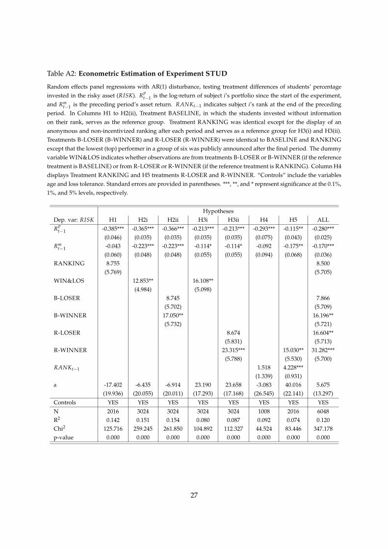
Table A2: Econometric Estimation of Experiment STUD

Random effects panel regressions with AR(1) disturbance, testing treatment differences of students’ percentageinvested in the risky asset (RISK). Rp

t−1 is the log-return of subject i’s portfolio since the start of the experiment,and Rm

t−1 is the preceding period’s asset return. RANKt−1 indicates subject i’s rank at the end of the precedingperiod. In Columns H1 to H2(ii), Treatment BASELINE, in which the students invested without informationon their rank, serves as the reference group. Treatment RANKING was identical except for the display of ananonymous and non-incentivized ranking after each period and serves as a reference group for H3(i) and H3(ii).Treatments B-LOSER (B-WINNER) and R-LOSER (R-WINNER) were identical to BASELINE and RANKINGexcept that the lowest (top) performer in a group of six was publicly announced after the final period. The dummyvariable WIN&LOS indicates whether observations are from treatments B-LOSER or B-WINNER (if the referencetreatment is BASELINE) or from R-LOSER or R-WINNER (if the reference treatment is RANKING). Column H4displays Treatment RANKING and H5 treatments R-LOSER and R-WINNER. “Controls” include the variablesage and loss tolerance. Standard errors are provided in parentheses. ***, **, and * represent significance at the 0.1%,1%, and 5% levels, respectively.

HypothesesDep. var: RISK H1 H2i H2ii H3i H3ii H4 H5 ALLRp

t−1 -0.385*** -0.365*** -0.366*** -0.213*** -0.213*** -0.293*** -0.115** -0.280***(0.046) (0.035) (0.035) (0.035) (0.035) (0.075) (0.043) (0.025)

Rmt−1 -0.043 -0.223*** -0.223*** -0.114* -0.114* -0.092 -0.175** -0.170***

(0.060) (0.048) (0.048) (0.055) (0.055) (0.094) (0.068) (0.036)RANKING 8.755 8.500

(5.769) (5.705)WIN&LOS 12.853** 16.108**

(4.984) (5.098)B-LOSER 8.745 7.866

(5.702) (5.709)B-WINNER 17.050** 16.196**

(5.732) (5.721)R-LOSER 8.674 16.604**

(5.831) (5.713)R-WINNER 23.315*** 15.030** 31.282***

(5.788) (5.530) (5.700)RANKt−1 1.518 4.228***

(1.339) (0.931)α -17.402 -6.435 -6.914 23.190 23.658 -3.083 40.016 5.675

(19.936) (20.055) (20.011) (17.293) (17.168) (26.545) (22.141) (13.297)Controls YES YES YES YES YES YES YES YESN 2016 3024 3024 3024 3024 1008 2016 6048R2 0.142 0.151 0.154 0.080 0.087 0.092 0.074 0.120Chi2 125.716 259.245 261.850 104.892 112.327 44.524 83.446 347.178p-value 0.000 0.000 0.000 0.000 0.000 0.000 0.000 0.000

27

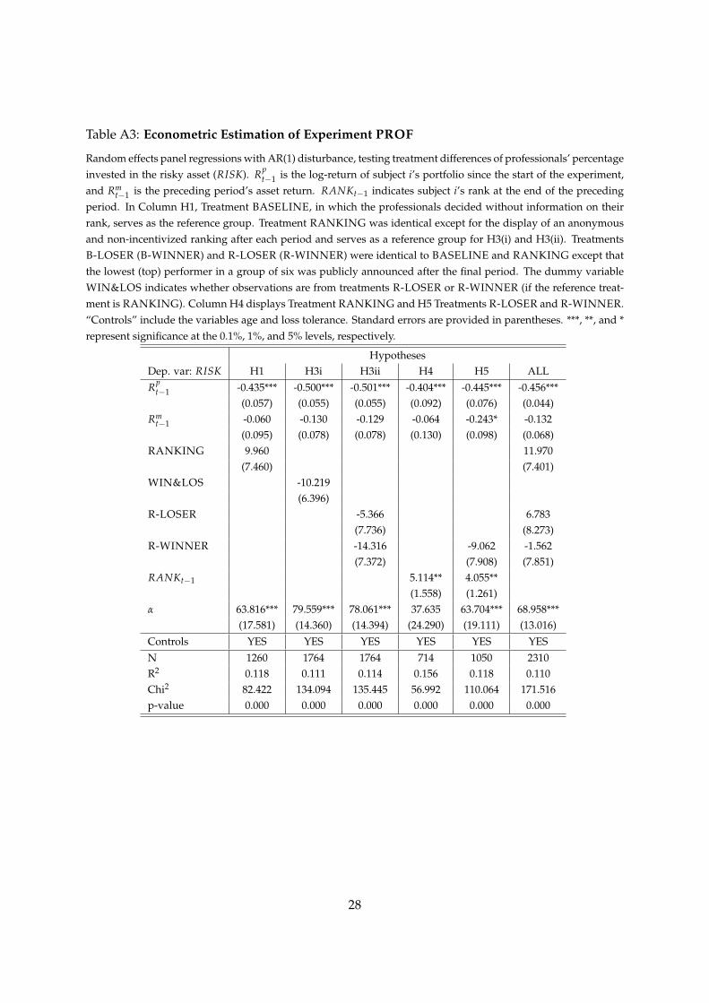
Table A3: Econometric Estimation of Experiment PROF

Random effects panel regressions with AR(1) disturbance, testing treatment differences of professionals’ percentageinvested in the risky asset (RISK). Rp

t−1 is the log-return of subject i’s portfolio since the start of the experiment,and Rm

t−1 is the preceding period’s asset return. RANKt−1 indicates subject i’s rank at the end of the precedingperiod. In Column H1, Treatment BASELINE, in which the professionals decided without information on theirrank, serves as the reference group. Treatment RANKING was identical except for the display of an anonymousand non-incentivized ranking after each period and serves as a reference group for H3(i) and H3(ii). TreatmentsB-LOSER (B-WINNER) and R-LOSER (R-WINNER) were identical to BASELINE and RANKING except thatthe lowest (top) performer in a group of six was publicly announced after the final period. The dummy variableWIN&LOS indicates whether observations are from treatments R-LOSER or R-WINNER (if the reference treat-ment is RANKING). Column H4 displays Treatment RANKING and H5 Treatments R-LOSER and R-WINNER.“Controls” include the variables age and loss tolerance. Standard errors are provided in parentheses. ***, **, and *represent significance at the 0.1%, 1%, and 5% levels, respectively.

HypothesesDep. var: RISK H1 H3i H3ii H4 H5 ALLRp

t−1 -0.435*** -0.500*** -0.501*** -0.404*** -0.445*** -0.456***(0.057) (0.055) (0.055) (0.092) (0.076) (0.044)

Rmt−1 -0.060 -0.130 -0.129 -0.064 -0.243* -0.132

(0.095) (0.078) (0.078) (0.130) (0.098) (0.068)RANKING 9.960 11.970

(7.460) (7.401)WIN&LOS -10.219

(6.396)R-LOSER -5.366 6.783

(7.736) (8.273)R-WINNER -14.316 -9.062 -1.562

(7.372) (7.908) (7.851)RANKt−1 5.114** 4.055**

(1.558) (1.261)α 63.816*** 79.559*** 78.061*** 37.635 63.704*** 68.958***

(17.581) (14.360) (14.394) (24.290) (19.111) (13.016)Controls YES YES YES YES YES YESN 1260 1764 1764 714 1050 2310R2 0.118 0.111 0.114 0.156 0.118 0.110Chi2 82.422 134.094 135.445 56.992 110.064 171.516p-value 0.000 0.000 0.000 0.000 0.000 0.000

28

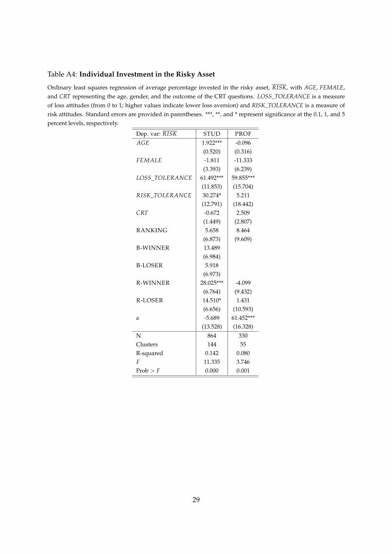
Table A4: Individual Investment in the Risky Asset

Ordinary least squares regression of average percentage invested in the risky asset, RISK, with AGE, FEMALE,and CRT representing the age, gender, and the outcome of the CRT questions. LOSS_TOLERANCE is a measureof loss attitudes (from 0 to 1; higher values indicate lower loss aversion) and RISK_TOLERANCE is a measure ofrisk attitudes. Standard errors are provided in parentheses. ***, **, and * represent significance at the 0.1, 1, and 5percent levels, respectively.

Dep. var: RISK STUD PROFAGE 1.922*** -0.096

(0.520) (0.316)FEMALE -1.811 -11.333

(3.393) (6.239)LOSS_TOLERANCE 61.492*** 59.855***

(11.853) (15.704)RISK_TOLERANCE 30.274* 5.211

(12.791) (18.442)CRT -0.672 2.509

(1.449) (2.807)RANKING 5.658 8.464

(6.873) (9.609)B-WINNER 13.489

(6.984)B-LOSER 5.918

(6.973)R-WINNER 28.025*** -4.099

(6.764) (9.432)R-LOSER 14.510* 1.431

(6.656) (10.593)α -5.689 61.452***

(13.528) (16.328)N 864 330Clusters 144 55R-squared 0.142 0.080F 11.335 3.746Prob > F 0.000 0.001

29

A2 Pictures of the Experimental Laboratories

Figure A2: Top: Example of a mobile laboratory in the conference room of a financial institu-tion. Bottom: Innsbruck EconLab.

30

A3 Modified CRT Questions

• An IT company offers you storage space. Every day your volume of data doubles. If itwould need 20 days to max out the provided space, how long would it take to max outhalf of the space?

• A football shoe and a ball cost 110 euro together. The shoe costs 70 euro more than theball. How much costs the ball?

• 5 machines need 5 minutes to produce 5 keyboards. How long would 80 machines needfor 80 keyboards?

31

ONLINE APPENDIXInstructions of the Experiment23

Welcome to the experiment and thank you for your participation!Please do not talk with the other participants during the experiment from now on.

General Information

In this experiment we study economic decision-making. The whole experiment consistsof two independent parts, where you can earn money independently. For your punctual at-tendance and participation you will receive a participation fee of 18 euro in addition to theincome you can earn in both parts of the experiment. Your entire payment will be paid out toyou privately and in cash after the experiment. At the beginning of each part you will receivedetailed instructions. If you have questions about the instructions or during the experiment,please raise your hand. One of the experimenters will then come to you and answer yourquestions privately.

PART 1

Task

In Part 1 you have to make investment decisions in a financial market. At the beginning ofthe experiment, you start with a wealth of 90 euro. You have to decide in each of eight periods(half-years), what percentage of your wealth you want to invest at a risk-free rate of 1.5% andthe percentage you wish to invest in a stock index. The development of the stock index reflectsthe price development of a basket of shares and is based on actual historical data. In the last 20years, this development is characterized by price fluctuations. In this period, the index earneda half-year return (semi-annual compounding) of 3.6% and had a standard deviation of thesemi-annual price returns of 15.9%.

Here are some examples on the likelihood of various price fluctuations:In 50 out of 100 cases, the semi-annual return lies between -7.1% and 14.3%.In 90 out of 100 cases, the semi-annual return lies between -22.6% and 29.8%.In 95 out of 100 cases, the semi-annual return lies between -27.6% and 34.7%.At the beginning of the first period, you have to draw 30 times from this distribution (at

your laptop) with a mean of 3.6% and a standard deviation of 15.9%. The draws are indepen-dent for each participant. After each draw the last drawn return is indicated on the screen witha yellow box together with the display of return (see Figure A3).

23Instructions are for Treatment BASELINE for the professional sample. Additional text for TreatmentsB-WINNER, RANKING, R-WINNER are outlined. The equivalent parts for treatments with public announce-ment of the worst performer (B-LOSER and R-LOSER) are made analogously and can be provided upon request.Note that instructions for the student sample are identical except that they only received one-third of the monetaryincentives.

32

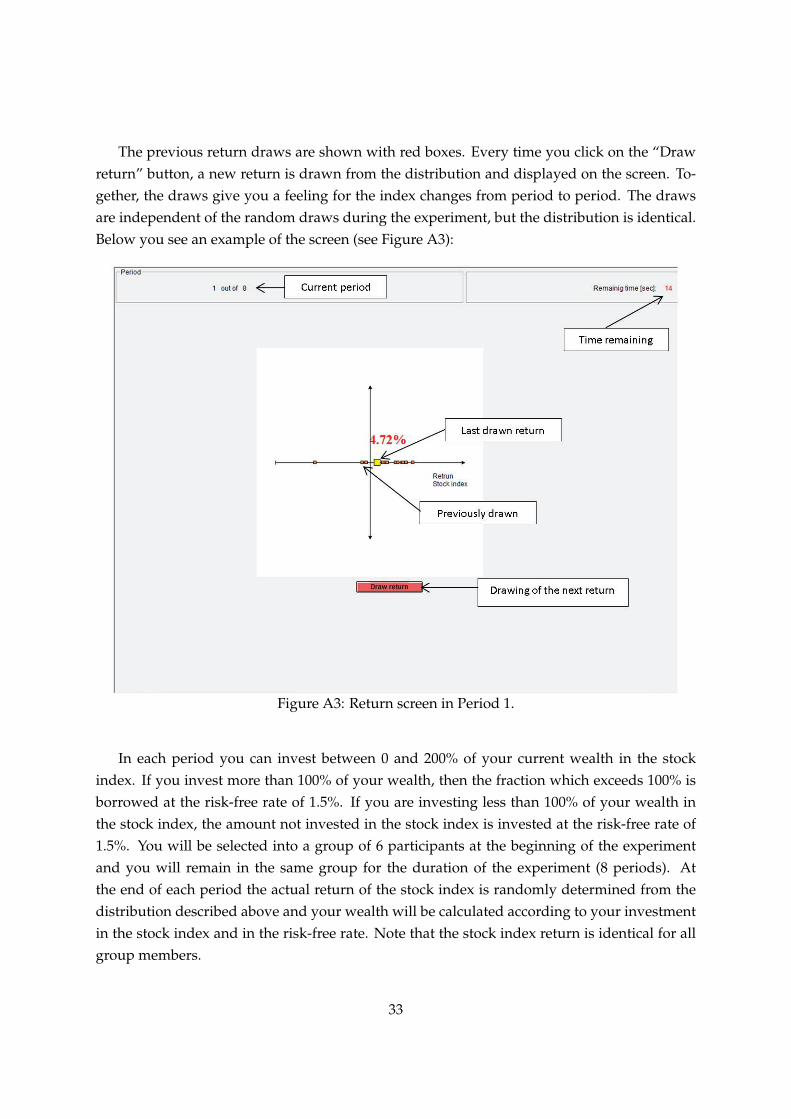
The previous return draws are shown with red boxes. Every time you click on the “Drawreturn” button, a new return is drawn from the distribution and displayed on the screen. To-gether, the draws give you a feeling for the index changes from period to period. The drawsare independent of the random draws during the experiment, but the distribution is identical.Below you see an example of the screen (see Figure A3):

Figure A3: Return screen in Period 1.

In each period you can invest between 0 and 200% of your current wealth in the stockindex. If you invest more than 100% of your wealth, then the fraction which exceeds 100% isborrowed at the risk-free rate of 1.5%. If you are investing less than 100% of your wealth inthe stock index, the amount not invested in the stock index is invested at the risk-free rate of1.5%. You will be selected into a group of 6 participants at the beginning of the experimentand you will remain in the same group for the duration of the experiment (8 periods). Atthe end of each period the actual return of the stock index is randomly determined from thedistribution described above and your wealth will be calculated according to your investmentin the stock index and in the risk-free rate. Note that the stock index return is identical for allgroup members.

33

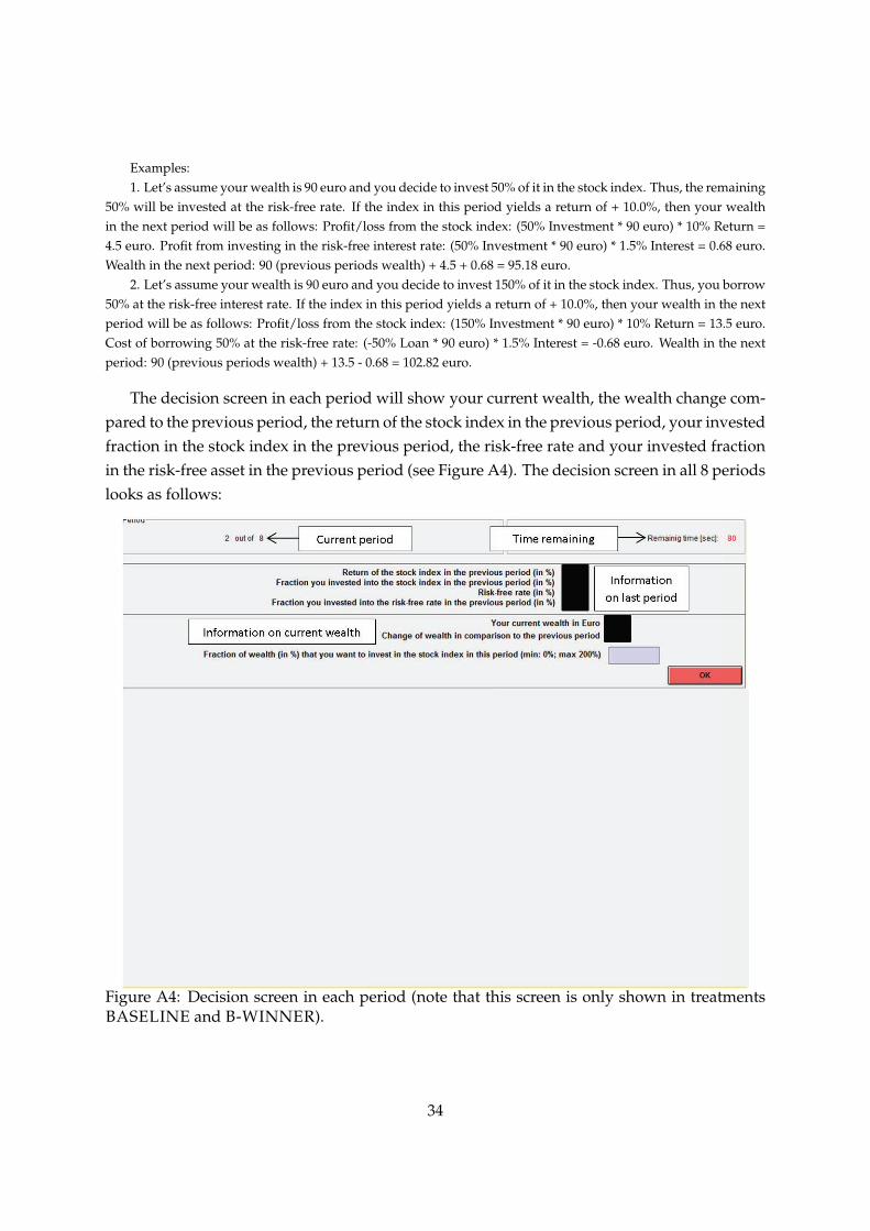
Examples:1. Let’s assume your wealth is 90 euro and you decide to invest 50% of it in the stock index. Thus, the remaining

50% will be invested at the risk-free rate. If the index in this period yields a return of + 10.0%, then your wealthin the next period will be as follows: Profit/loss from the stock index: (50% Investment * 90 euro) * 10% Return =4.5 euro. Profit from investing in the risk-free interest rate: (50% Investment * 90 euro) * 1.5% Interest = 0.68 euro.Wealth in the next period: 90 (previous periods wealth) + 4.5 + 0.68 = 95.18 euro.

2. Let’s assume your wealth is 90 euro and you decide to invest 150% of it in the stock index. Thus, you borrow50% at the risk-free interest rate. If the index in this period yields a return of + 10.0%, then your wealth in the nextperiod will be as follows: Profit/loss from the stock index: (150% Investment * 90 euro) * 10% Return = 13.5 euro.Cost of borrowing 50% at the risk-free rate: (-50% Loan * 90 euro) * 1.5% Interest = -0.68 euro. Wealth in the nextperiod: 90 (previous periods wealth) + 13.5 - 0.68 = 102.82 euro.

The decision screen in each period will show your current wealth, the wealth change com-pared to the previous period, the return of the stock index in the previous period, your investedfraction in the stock index in the previous period, the risk-free rate and your invested fractionin the risk-free asset in the previous period (see Figure A4). The decision screen in all 8 periodslooks as follows:

Figure A4: Decision screen in each period (note that this screen is only shown in treatmentsBASELINE and B-WINNER).

34

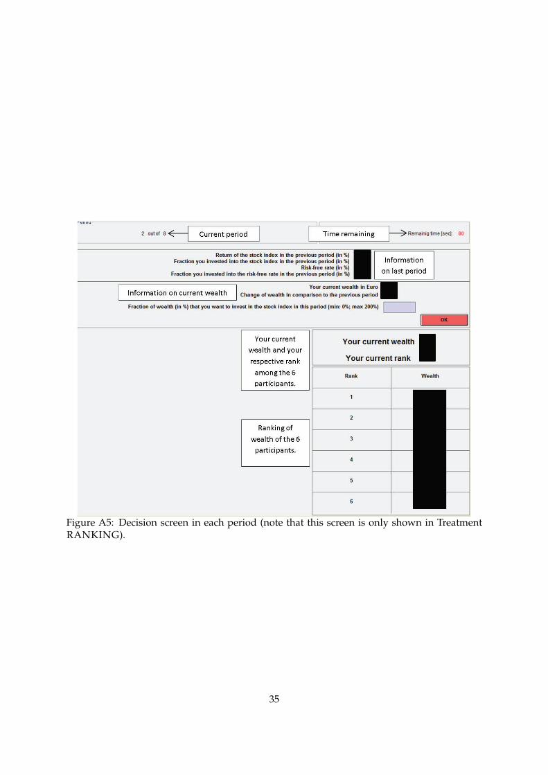
Figure A5: Decision screen in each period (note that this screen is only shown in TreatmentRANKING).

35

�

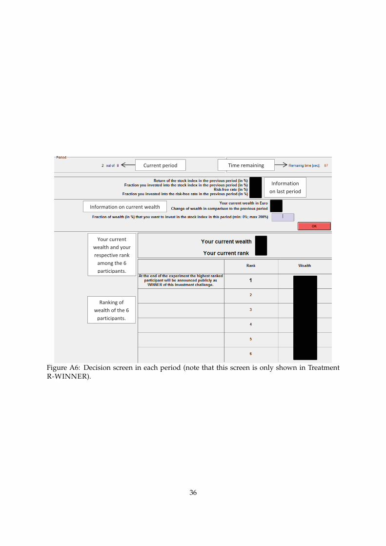
Information�on�last�period�

Time�remainingCurrent�period

Information�on�current�wealth�

Ranking�of�wealth�of�the�6�

participants.�

Your�current�wealth�and�your�respective�rank�

among�the�6�participants.�

Figure A6: Decision screen in each period (note that this screen is only shown in TreatmentR-WINNER).

36

[Begin additional text for Treatments RANKING and R-WINNER]Beginning with Period 2, you will be informed in a league table which rank in your group of 6

you currently have based on the current wealth of the participants. You also get information about thecurrent wealth and rank of the other participants in your group. This table appears for 20 seconds at thebeginning of each period (see Figure A7) and is also displayed at the bottom of the decision screen (seeFigure A5).

[End additional text for Treatments RANKING and R-WINNER]

[Begin text for Treatment B-WINNER]

Public announcement of the winner in each group

At the end of the experiment (before you receive your payment) the highest ranked participant ineach group (of 6 participants) will be announced to all participants in the room as WINNER of thisinvestment challenge.

[End text for Treatment B-WINNER]

[Begin text for Treatment R-WINNER]

Public announcement of the winner in each group

As you see in figures A6 and A8, the first place is highlighted. The reason is that at the end ofthe experiment (before you receive your payment) the highest ranked participant in each group (of 6participants) will be announced to all participants in the room as WINNER of this investment challenge.

[End text for Treatment R-WINNER]

37

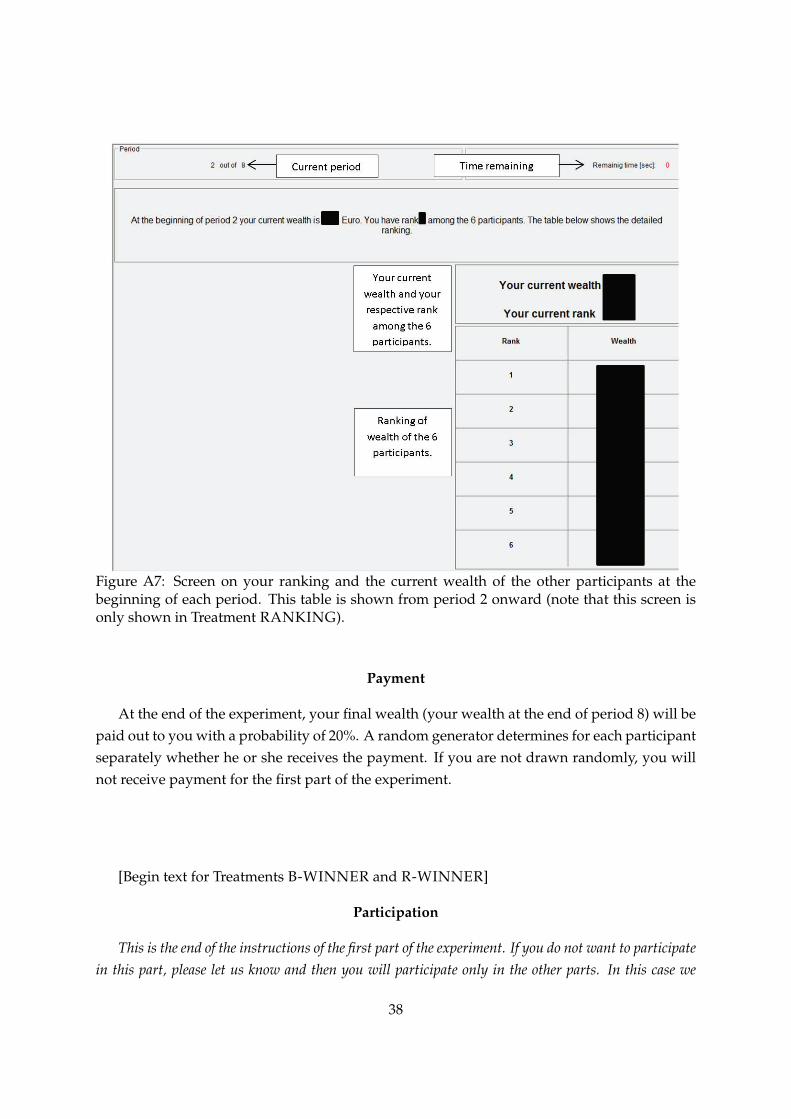
Figure A7: Screen on your ranking and the current wealth of the other participants at thebeginning of each period. This table is shown from period 2 onward (note that this screen isonly shown in Treatment RANKING).

Payment

At the end of the experiment, your final wealth (your wealth at the end of period 8) will bepaid out to you with a probability of 20%. A random generator determines for each participantseparately whether he or she receives the payment. If you are not drawn randomly, you willnot receive payment for the first part of the experiment.

[Begin text for Treatments B-WINNER and R-WINNER]

Participation

This is the end of the instructions of the first part of the experiment. If you do not want to participatein this part, please let us know and then you will participate only in the other parts. In this case we

38

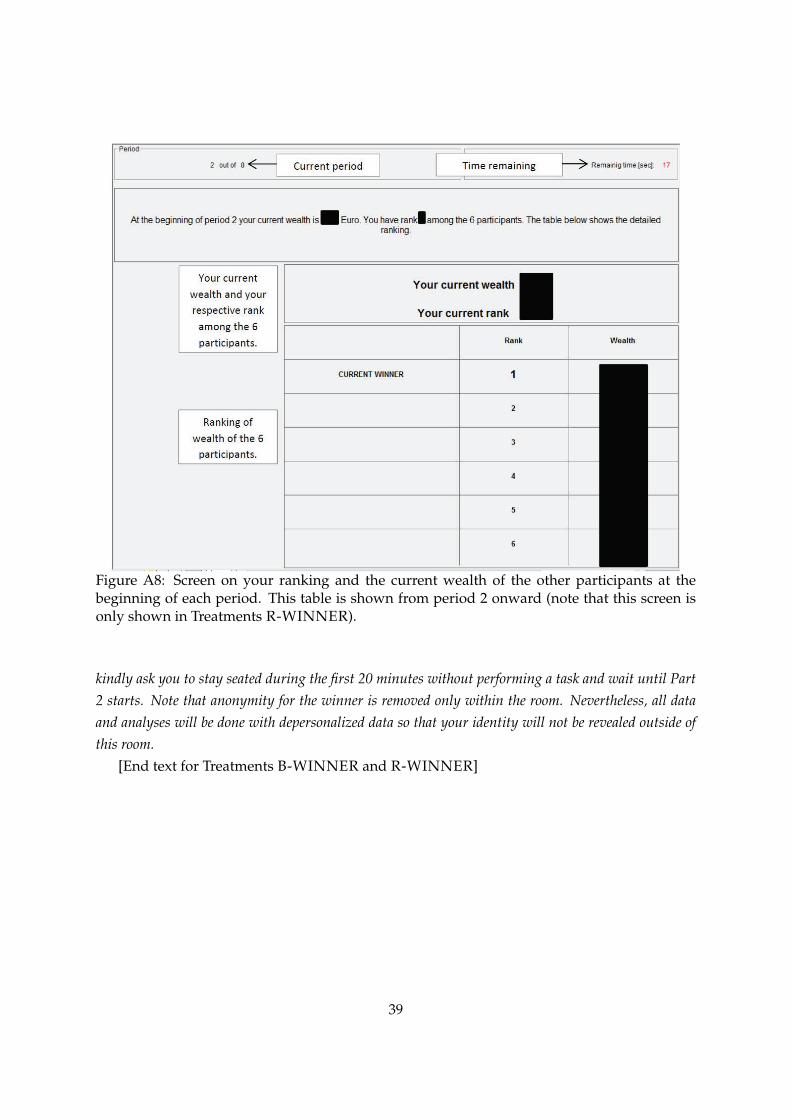
Figure A8: Screen on your ranking and the current wealth of the other participants at thebeginning of each period. This table is shown from period 2 onward (note that this screen isonly shown in Treatments R-WINNER).

kindly ask you to stay seated during the first 20 minutes without performing a task and wait until Part2 starts. Note that anonymity for the winner is removed only within the room. Nevertheless, all dataand analyses will be done with depersonalized data so that your identity will not be revealed outside ofthis room.

[End text for Treatments B-WINNER and R-WINNER]

39

PART 2Below are the instructions for Part 2 of this experiment.

Remember: You get 18 euro for participating in this experiment. In Part 2, you can earn(and lose) in addition to this participation fee. Part 1 and Part 2 are independent in the deci-sions and in payment.

Part 2 consists of two sections that are played one after the other. For each of the twosections, your potential payment will be calculated individually and independently. At theend of Part 2 one of the two sections will be randomly selected for your payment for Part 2 (fordetails on payment, see below).

Section 1

In Section 1, you are asked to make 7 decisions (decision pairs). For each decision pair, youhave the choice between Option A and Option B:

OPTION A: A payment with 100% probability (certainty) is realized. This option is avail-able in all seven decision pairs.

OPTION B: A payment that is risky – either 0 euro with 50% probability or 24 euro with50% probability.

For your payment, ONE out of the 7 decision pairs will be randomly selected and used forpayment according to your decision.

Section 2

In the 6 questions of Section 2 you have to decide whether you want to participate in alottery where you can win or lose money. If you choose the lottery, the computer flips a coin.If the coin shows heads, you get 15 euro in addition to your participation fee. If the coin showstails, you lose a certain amount of your participation fee. If you do not choose the lottery, youwill receive 0 euro in addition to your participation fees.

For your payment, ONE out of the 6 decision pairs will be randomly selected and used forpayment according to your decision.

In Part 2, one of the two sections will be randomly selected and paid out at the end ofthe experiment; in addition to the participation fee and in addition to the payment of Part 1.Please note: In Part 2, next to playing out a possible lottery, there is a maximum of two randomdrawings. The first random draw is used to select which section is relevant for your payment.In a second step, one of the decision pairs will be randomly chosen from the relevant section.Your decision (lottery or fixed payment) is then played out to determine your payment.

Questionnaire

40

Following Part 2 you will be asked to answer some general questions and provide us withsome anonymous demographic details.

Thank you for your participation!

41

University of Innsbruck - Working Papers in Economics and StatisticsRecent Papers can be accessed on the following webpage:

https://www.uibk.ac.at/eeecon/wopec/

2019-07 Florian Lindner, Michael Kirchler, Stephanie Rosenkranz, UtzeWeitzel: Social Mo-tives and Risk-Taking in Investment Decisions

2019-06 Christoph Huber, Julia Rose: Individual attitudes and market dynamics towardsimprecision

2019-05 Felix Holzmeister, Jürgen Huber, Michael Kirchler, Florian Lindner, Utz Weitzel,Stefan Zeisberger: What Drives Risk Perception? A Global Survey with FinancialProfessionals and Lay People

2019-04 David M. McEvoy, Tobias Haller, Esther Blanco: The Role of Non-Binding Pledgesin Social Dilemmas with Mitigation and Adaptation

2019-03 KatharinaMomsen,MarkusOhndorf:Whendopeople exploitmoralwiggle room?An experimental analysis in a market setup

2019-02 Rudolf Kerschbamer, Daniel Neururer, Matthias Sutter: Credence goods marketsand the informational value of new media: A natural field experiment

2019-01 Martin Geiger, Eric Mayer, Johann Scharler: Inequality and the Business Cycle:Evidence from U.S. survey data

2018-18 Matthias Sutter, Jürgen Huber, Michael Kirchler, Matthias Stefan, Markus Walzl:Where to look for the morals in markets?

2018-17 Rene Schwaiger, Michael Kirchler, Florian Lindner, Utz Weitzel: Determinants ofinvestor expectations and satisfaction. A study with financial professionals

2018-16 Andreas Groll, Julien Hambuckers, Thomas Kneib, Nikolaus Umlauf: LASSO-TypePenalization in the Framework of Generalized Additive Models for Location, Scaleand Shape

2018-15 Christoph Huber, Jürgen Huber: Scale matters: Risk perception, return expecta-tions, and investment propensity under different scalings

2018-14 Thorsten Simon, Georg J. Mayr, Nikolaus Umlauf, Achim Zeileis: Lightning predic-tion using model output statistics

2018-13 Martin Geiger, Johann Scharler: How do consumers interpret the macroeconomiceffects of oil price fluctuations? Evidence from U.S. survey data

2018-12 Martin Geiger, Johann Scharler: How do people interpret macroeconomic shocks?Evidence from U.S. survey data

2018-11 Sebastian J. Dietz, Philipp Kneringer, Georg J. Mayr, Achim Zeileis: Low visibilityforecasts for different flight planning horizons using tree-based boosting models

2018-10 Michael Pfaffermayr: Trade creation and trade diversion of regional trade agree-ments revisited: A constrained panel pseudo-maximum likelihood approach

2018-09 Achim Zeileis, Christoph Leitner, Kurt Hornik: Probabilistic forecasts for the 2018FIFA World Cup based on the bookmaker consensus model

2018-08 Lisa Schlosser, Torsten Hothorn, Reto Stauffer, Achim Zeileis: Distributional re-gression forests for probabilistic precipitation forecasting in complex terrain

2018-07 Michael Kirchler, Florian Lindner, Utz Weitzel: Delegated decision making and so-cial competition in the finance industry

2018-06 Manuel Gebetsberger, Reto Stauffer, Georg J.Mayr, Achim Zeileis: Skewed logisticdistribution for statistical temperature post-processing in mountainous areas

2018-05 Reto Stauffer, Georg J.Mayr, JakobW.Messner, Achim Zeileis: Hourly probabilisticsnow forecasts over complex terrain: A hybrid ensemble postprocessing approach

2018-04 Utz Weitzel, Christoph Huber, Florian Lindner, Jürgen Huber, Julia Rose, MichaelKirchler: Bubbles and financial professionals

2018-03 Carolin Strobl, Julia Kopf, Raphael Hartmann, Achim Zeileis: Anchor point selec-tion: An approach for anchoring without anchor items

2018-02 Michael Greinecker, Christopher Kah: Pairwise stablematching in large economies

2018-01 Max Breitenlechner, Johann Scharler: How does monetary policy influence banklending? Evidence from the market for banks’ wholesale funding

University of Innsbruck

Working Papers in Economics and Statistics

2019-07

Florian Lindner, Michael Kirchler, Stephanie Rosenkranz, Utz Weitzel

Social Motives and Risk-Taking in Investment Decisions

AbstractA pervasive feature in the finance industry is relative performance, which can includeextrinsic (money), intrinsic (self-image), and reputational (status) motives. In this paper,we model a portfolio decision with two assets and investigate how reputational motives(i.e., the public announcement of the winners or losers) influence risk-taking in invest-ment decisions vis-a-vis intrinsic motives. We test our hypotheses experimentally with864 students and 330 financial professionals. We find that reputational motives play aminor role among financial professionals, as the risk-taking of underperformers is alreadyincreased due to intrinsicmotives. Student behavior, however, ismainly driven by reputa-tional motives with risk-taking levels that come close to those of professionals when win-ners or losers are announced publicly. This indicates that professionals show higher levelsof intrinsic (self-image) incentives to outperform others compared to non-professionals(students), but a similar behavior can be sparked among the latter by adding reputationalincentives.

ISSN 1993-4378 (Print)ISSN 1993-6885 (Online)