Embed Size (px)
Citation preview
Social Networks and Migration:Theory and Evidence from Rwanda
Joshua Blumenstock∗
University of California, Berkeley
Xu Tan†
University of Washington
December 2016
PRELIMINARY - DO NOT CITE OR CIRCULATE WITHOUT PERMISSION
Abstract
How does the structure of an individual’s social network affect his decision to mi-grate? We study the migration decisions of over one million individuals in Rwanda overa period of several years, using novel data from the monopoly mobile phone operatorto reconstruct the complete social network of each individual in the months prior tomigration. We use these data to directly validate several classic theories of migrationthat have historically been difficult to test, for instance that individuals with closely-knit networks in destination communities are more likely to migrate. Our analysis alsouncovers several empirical results that have not been documented in the prior liter-ature, and which are not consistent with common theories of how individuals derivevalue from their social networks. We propose a simple model of strategic cooperationto reconcile these results.
∗University of California, Berkeley, [email protected]†University of Washington, [email protected]
1
1 Introduction
Migrants play a central role in bringing an economy towards a more efficient use of its re-
sources. In many contexts, however, a range of market failures limit the extent to which
people can capitalize on opportunities for arbitrage through migration. Recent literature
documents, for instance, cases where information does not reach the migrant (Jensen, 2012),
households lack insurance against the risk of migration (Bryan, Chowdhury and Mobarak,
2014), and source communities discourage exit (Beegle, De Weerdt and Dercon, 2010, Munshi
and Rosenzweig, 2016). The resulting underinvestment in migration leads to the misalloca-
tion of capital, and can have severe consequences for the overall economy.1
The decision to migrate depends on the extent to which the migrant is connected to
communities and home and in the destination. Much of the existing literature has focused on
how strong ties to the destination community can facilitate migration by providing access to
information about jobs (Munshi, 2003, Borjas, 1992) and material support for reecent arrivals
(Munshi, 2014). The role of the home network is more ambiguous. On the one hand, robust
risk sharing networks can partially insure against the risk of temporary migration (Morten,
2015), making it easier for people to leave. On the other hand, strong source networks can
also discourage permanent migration if migrant households are subsequently excluded from
risk sharing networks.
While there is thus general consensus that social networks play an important role in
migration decisions, the exact nature of this role is unclear. This ambiguity stems, at
least in part, from a lack of reliable data on both migration and the structure of social
networks. Migration is difficult to measure, particularly in developing countries where short-
term migration is common and reliable household survey data is limited (McKenzie and
Sasin, 2007, Carletto, de Brauw and Banerjee, 2012, Lucas, 2015). Social network structure
is even harder to observe. Recent empirical work on networks relies on survey modules that
1Bryan, Chowdhury and Mobarak (2014), for instance, link underinvestment in migration to seasonalfamine. Munshi and Rosenzweig (2006) and McKenzie and Rapoport (2007) show how migration can affectinequality and the distribution of income.
2
ask respondents to list their social connections, but this approach is necessarily limited in
scope and scale. Thus, much of the literature on networks and migration relies on indirect
information on social networks, such as the (plausible) assumption that individuals from the
same hometown, or with similar observable characteristics, are more likely to be connected
that two dissimilar individuals.
We leverage a novel source of data to provide detailed insight into the role of social
networks in the decision to migrate. Using several years of data capturing the entire universe
of mobile phone activity in Rwanda, we track the internal migration decisions of roughly
one million unique individuals, as inferred from the locations of the cellular towers they use
to make and receive phone calls. We link these migration decisions to the structure of each
migrant’s social network, as inferred from the set of people with whom he or she interacts
over the phone network. Merging the geospatial and network data, we observe the migrant’s
connections to his home community, his connections to all possible destination communities,
as well as the complete higher-order structure of the network (i.e., the connections of the
migrant’s connections).
To structure our analysis, we develop a strategic cooperation model to characterize how an
individual can obtain value from her social network. This “social value” is broadly construed
to capture access to information and opportunities for risk sharing and favor exchange.
Within our repeated cooperation setting, agents randomly meet their connected neighbors
over time, and when two agents meet, they each contribute effort to a joint project. Effort
is determined endogenously by the network structure, so the model allows us to describe in
equilibrium how network structure affects the social value that agents get from the network,
which in turn affects the decision to migrate.2
The model generates several intuitive predictions that are documented in prior work, and
which are also reflected in our data. Namely, agents receive higher utility when their network
2See Ali and Miller (2016) for a related approach, which builds on past observations that social sanctionscan improve commitment in risk sharing (Chandrasekhar, Kinnan and Larreguy, 2014, Karlan et al., 2009)and may strengthen job referral networks (Heath, 2016).
3
has a larger number of contacts, and when the frequency of interaction with neighbors is
increased. This is consistent with several studies linking exogenously larger social networks
in the destination to higher rates of migration (cf. Munshi, 2003). And in our data, we
indeed see that rates of migration are increasing in the number of contacts an individual
has in a destination community, and in the frequency of interaction with those contacts.
Similarly, our model predicts that stronger networks in the home community will make a
migrant less likely to leave, which is consistent with a story where individuals fear being
ostracized from inter-family insurance networks (Munshi and Rosenzweig, 2016). Our data
indicate a decreasing, monotonic, and approximately linear relationship between migration
rates and the extent of the home network.
More interesting, our model and data make it possible to generate and test several hy-
potheses about the role of social networks in migration that the existing literature has been
unable to explore. Notably, we show that social connections generate positive externalities.
That is, if two agents form a link or increase their interaction over the existing link, their
common neighbors (in addition to themselves) receive strictly higher utilities from the net-
work. This generates the testable predictions that an agent should be more likely to migrate
if her connections in the destination form more links among themselves; and if the frequency
of interaction between common neighbors increases. As we show, each of these predictions is
supported by the data, although the shape of the migration response function is not always
linear or monotonic.
We also document - to our knowledge for the first time - the role that more distant
network connections play in migration. Superficially, we find that an individual is more
likely to migrate to a destination where his friends have more friends. However, this effect
does not persist after controlling for the number of friends in the destination; instead, the
marginal effect of second-order friends conditional on first-order friends is somewhat negative.
For example, if both Joe and Jane have the same number of contacts living in a destination
community, but Joe’s contacts have more contacts in the destination than Jane’s contacts
4
do, it is (counterintuitively) Jane who is more likely to migrate.
Taken together, these results allow us to differentiate between two common approaches
to modeling the economic value of social networks. In particular, we contrast the predictions
of the strategic cooperation model described above with a simple model of information
diffusion (e.g., Banerjee et al., 2013). The strategic cooperation model is consistent with
both externalities observed in the data. This is because in the cooperation game, the agent
is not aware of the action of her neighbors’ neighbors, therefore her endogenous effort depends
only on the actions and structure of her immediate network. The key assumption – that the
individual does not have knowledge about the network outside of her immediate neighbors
– is a consistent finding in the empirical literature (see, for example Krackhardt, 1990,
Casciaro, 1998, Chandrasekhar, Breza and Tahbaz-Salehi, 2016). By contrast, most models
of information diffusion predict that positive externalities would be global. As information is
shared more often somewhere in the network, an agent is more likely to hear about it faster,
and the marginal effect of second order friends should be strictly positive. This prediction
is not supported by the data, which implies that the information diffusion model cannot be
the sole determinant of network value in the context of migration.
Our final set of results explores heterogeneity in the migration response to social network
structure. We separately study the role of the network in migration between and across
rural and urban areas, in short- and long-distance moves, and in temporary vs. permanent
migrations. While the main effects described above are generally consistent in each of these
sub-populations, the shape and magnitude of the migration response differs significantly by
migration type.
Since our approach to studying migration with mobile phone data is new, we perform a
large number of specification tests to calibrate for likely sources of measurement error and
to test the robustness of our results. In particular, one limitation of our approach is that
we lack exogenous variation in the structure of an individual’s network, so that network
structure may be endogenous to decisions regarding migration. We address this concern in
5
two principal ways. First, we derive structural properties of the migrant’s social network
in the period prior to migration. Our results change little even when we reconstruct each
migrant’s social network using communications data from several months prior to the date
of migration. Second, we leverage the vast quantity of data at our disposal to control for a
robust set of network characteristics and better isolate the structural parameter of interest.
For instance, we condition on the number of common neighbors when analyzing the effect
of the frequency of communication between common neighbors. Thus, while having a large
number of contacts in a destination may be endogenous to migration, and likely migrants
may even select contacts who are connected to each other, we assume migrants will be less
able to control the extent to which those contacts communicate.
This paper makes two primary contributions. First, we contribute to a growing literature
on the economic value of social networks (cf. Jackson, Rodriguez-Barraquer and Tan, 2012,
Banerjee et al., 2013, 2014). Our model connects this literature to research on migration in
developing countries, and indicates that a model of social support is more consistent with
the data than a model of information diffusion. Second, we contribute to empirical research
on the determinants of internal migration in developing countries (cf. Bryan, Chowdhury
and Mobarak, 2014, Morten, 2015, Lucas, 2015). In this literature, it has historically been
difficult to measure the effect of social networks in migration; our data make it possible to
directly test several conjectures in the prior literature, and to develop new insight into the
relationship between social network structure and the decision to migrate.
2 A strategic model of migration
People need their friends’ help and support when moving and settling down in a new place.
We model the decision to migrate as a function of the utility an agent receives from neighbors
in the network. In particular, agents play cooperation games with their neighbors repeatedly
over time, and the utility they get can represent the level of support they obtain from the
6
network. The model provides micro foundations for several stylized empirical predictions,
which we can bring to the data. Moreover, it deviates in important ways from alternative
models of migration in social networks, for instance the information diffusion model which
we will discuss in Section 2.2.
2.1 A repeated cooperation game with neighbors
Consider a population of N players, N = {1, . . . , n}, who are connected in an undirected
network G, with ij ∈ G if agent i and j are connected. Denote agent i’s neighbors as
Ni = {j : ij ∈ G}, and her degree as di = |Ni|.
Each pair of connected agents, ij ∈ G, is engaged in a partnership ij that meets at
random times generated by a Poisson process of rate λij > 0. When they meet, agent i
and j choose their effort levels aij, aji in [0,∞) as their contributions to a joint project.3
Player i’s stage game payoff function when partnership ij meets is b(aji) − c(aij), where
b(aji) is the benefit from her partner j’s effort and c(aij) is the cost she incurs from her
own effort. The benefit function b and the cost function c are smooth functions satisfying
b(0) = c(0) = 0. All players share a common discount rate r > 0, and the game proceeds
over continuous time t ∈ [0,∞).
We write the net value of effort a as v(a) ≡ b(a)− c(a), and we assume that it grows in
the following manner.
Assumption 1. The net value of effort v(a) is strictly increasing and weakly concave, with
v(0) = 0. Moreover, v′(a) is uniformly bounded away from zero.
Assumption 1 implies that higher effort is always socially beneficial; concavity means
it is better for partners to exert similar effort, holding their average effort constant. The
following assumption articulates that higher effort levels increase the temptation to shirk.
Assumption 2. The cost of effort c is strictly increasing and strictly convex, with c(0) =
c′(0) = 0 and lima→∞ c′(a) =∞. The “relative cost” c(a)/v(a) is strictly increasing.
3The variable-stakes formulation is adopted from Ghosh and Ray (1996) and Ali and Miller (2016).
7

Strict convexity with the limit condition guarantees that in equilibrium effort is bounded
(as long as continuation payoffs are bounded, which we assume below). Increasing relative
cost means a player requires proportionally stronger incentives to exert higher effort.
As has been documented in several different real-world contexts, we assume agents have
only local knowledge of the network.4 Each agent only observes her local network, including
her neighbors and the links among them (in additional to her own links). To be precise,
agent i observes her neighbors in Ni and all links in Gi = {jk : j, k ∈ {i} ∪ Ni}. Similarly,
each agent learns about her neighbors’ deviation and we assume this information travels
instantly.
Homogenous meeting frequency
As a benchmark, we start with the case that λ is i.i.d. across agents. Following the definition
from Jackson, Rodriguez-Barraquer and Tan (2012), a link ij is supported if they have at
least one common neighbor k ∈ Ni ∩ Nj, and ij is m-supported if they have m common
neighbors. There are critical effort levels, for supported and unsupported links.
Unsupported cooperation. Consider a strategy profile in which each of i and j exerts effort
level a0, if each has done so in the past; otherwise, each exerts zero effort.
b(a0) ≤ v(a0) +
∫ ∞0
e−rtλv(a0)dt. (1)
The incentive constraint is binding at effort level a∗0.
Supported cooperation. Consider a triangle i, j, k and a strategy profile in which each of
them exerts effort level a1, if each has done so in the past; otherwise, each exerts zero effort.
b(a1) ≤ v(a1) + 2
∫ ∞0
e−rtλv(a1)dt. (2)
4Examples in the literature include Krackhardt (1990), Casciaro (1998) and Chandrasekhar, Breza andTahbaz-Salehi (2016).
8
The incentive constraint is binding at effort level a∗1. Notice that the future value of coopera-
tion is higher in a triangle, 2∫∞0e−rtλv(a1)dt, so it can sustain higher level of efforts a∗1 > a∗0
and everyone gets a strictly higher utility.
Higher-order supported cooperation. Let m(ij) = |Ni ∩Nj| be the number of agents who
are common neighbors of i and j. Consider i and j sharing m common neighbors and a
strategy profile in which each of them exerts effort level am if each has done so in the past;
otherwise, each exerts zero effort.
b(am) ≤ v(am) +
∫ ∞0
e−rtλ [v(am) +mv(a∗1)] dt, (3)
in which i and j assume other pairs cooperate on at least a∗1 when they are supported.
The incentive constraint is binding at effort level a∗m. Following the same argument, more
common neighbors can sustain a higher level of cooperation between i and j, that is a∗m
strictly increases in m.
We can now characterize a simple strategy profile, which satisfies two nice properties.5
First, it is measurable to local networks, such that the effort level between any pair of agents
only depends on the local networks they share. Second, it is strongly robust to social conta-
gion, such that any pair of agents should continue playing their strategy on the equilibrium
path if neither has deviated before. The strong robustness is particularly important because
agents do not need to worry about contagion of any deviation and can continue cooperating
with each other. However, it is not easy to satisfy. Notice that the ostracism type of punish-
ment agents use in equation (2) does not satisfy the strong robustness requirement, because
if i deviates, j and k no longer cooperate with each other at a∗1 level. To achieve strong
robustness, we need a social norm on how to punish a deviator. If agent i shirked on agent
j, the game between i and any of her neighbors, say k ∈ Ni, becomes sequential: Agent i
chooses an effort aGik first as the guilty agent, and then agent k observes i’s effort and chooses
5We use a simplified version of the strategy profile studied in Ali and Miller (2016), and later introduceheterogeneous meeting frequency to match with our data.
9

his effort aIki as the innocent partner. These effort levels are set to let the guilty agent get a
payoff of zero while the innocent agent get the same payoff as that on the equilibrium path.
b(aIki)− c(aGik) = 0, and b(aGik)− c(aIki) = v(aik).
There must exist a solution satisfying 0 < aIki < aGik < aik.
Strategy profile: Everyone starts off “innocent.” While innocent, agent i and j choose
simultaneously and they work at effort level aij = aji = a∗m(ij). If i shirked on j, i becomes
“guilty.” While guilty, the cooperation game between i and each of her neighbors becomes
the sequential one above. i moves first and chooses aGik, and then k ∈ Ni moves second and
chooses aIki only if i chose at least aGik, and k chooses 0 otherwise. Lastly, if someone in Ni
deviates while i is guilty, then i becomes innocent and her strategy with her neighbors goes
back to the simultaneous one, except she now starts to punish the new deviator.
Proposition 1. Consider the game with homogenous meeting frequency. There exists an
equilibrium, measurable to local networks and strongly robust to social contagion, in which
any pair of connected agents, say i and j, cooperate on a∗m(ij), where m(ij) = |Ni ∩Nj|.
All proofs are in Appendix A1. Intuitively, the more common neighbors a pair of agents
have, the higher utility they can get from their cooperation. That is, a∗m increases in the
number of common neighbors m. Thus, in the equilibrium above each agent gets a strictly
higher utility if she forms more links, or if her neighbors form more links among themselves.
To generalize this intuition, we now show that if an agent’s degree, support or clustering
increases,6 then she can get a higher utility from the network. In particular, while there
are many possible equilibria, we restrict our attention on those in which each agent gets a
positive expected payoff from each link.
Proposition 2. Consider two networks, G and G′ = G ∪ {ij} such that ij /∈ G. For any
6“Support” is defined as the fraction of one’s links that are supported; “clustering” is defined as thefraction of pairs of one’s neighbors that are connected.
10
equilibrium ΣG in network G, there is an equilibrium ΣG′ in network G′ weakly dominating
ΣG and for any agent k ∈ {i, j}∪ (Ni∩Nj) in network G, k must get a higher utility in ΣG′.
The proposition shows that each link not only benefits its two agents, but also exhibits
positive externalities. First of all, the link ij gives agent i and j each a higher utility due to
this new cooperation opportunity. As a result, they get a higher utility from cooperation and
thus they face a higher punishment if they deviate. This additional punishment then sustains
i and j’s incentives to cooperate at a higher level with their common neighbors k ∈ Ni ∩Nj,
who can observe the link. So k can get a higher utility once i and j are connected.
Heterogeneous meeting frequency
In the data, we can measure the communication frequency between any pair of agents.
To examine its effect on the utility one gets from the network, we now allow heterogeneous
meeting frequency, and λij is locally observed by i, j and their common neighbors in Ni∩Nj.
First, in a bilateral partnership, agents get a higher utility when they meet more of-
ten. Let a∗0(λij) be the unsupported effort level when only i and j are connected and
they meet with the frequency λij. The counterpart to equation (1) becomes b(a0) ≤
v(a0) +∫∞0e−rtλijv(a0)dt. The incentive constraint is binding at effort level a∗0(λij). It is
easy to verify that a∗0(λij) increases in λij, which implies as the meeting frequency increases,
the utility agent i and j can obtain from their cooperation increases.
This is also true in an arbitrary network, such that an agent can get a higher utility if her
interaction frequency with her neighbors increases and/or the interaction frequency between
two of her neighbors increases.
Proposition 3. Consider the game with heterogeneous meeting frequencies, and increase the
frequency on one and only one link λ′ij > λij, and equal for all other links. For any equilibrium
Σλ, there is an equilibrium Σλ′ weakly dominating Σλ and for any agent k ∈ {i, j}∪(Ni∩Nj),
k must get a higher utility in Σλ′.
11
The proposition shows that the interaction frequency also exhibits positive externalities.
As i and j meet more often, they each gets a higher utility from cooperation, which pro-
vides the incentive to not only contribute greater effort to their partnership ij, but also to
partnerships with their common friends k ∈ Ni ∩Nj. Thus, k receives a higher utility from
i and j as they meet more frequently.
However, the positive externalities found in Proposition 2 and Proposition 3 are local
effects to agents in {i, j}∪ (Ni ∩Nj). Other agents who only know either i or j do not know
whether ij are connected or their frequency of interaction. Thus, they cannot choose their
efforts based on the link ij, nor benefit from its existence or its increased frequency. This
type of local knowledge seems particularly relevant when a person is considering migrating to
a potential destination. Because an agent has not yet moved to the destination, it is unlikely
that she knows much beyond her immediate neighbors. This local positive externality differs
from the prediction of an information diffusion model outlined below.
2.2 An alternative model of information diffusion
People may also share information through the network about potential job opportunities in
the destination, which can affect the migration decision. There are several diffusion models
in the literature, including both mechanical communication and strategic communication
(see summaries in Jackson and Yariv (2010) and Banerjee et al. (2013)).
We begin with a mechanical diffusion model and allow for possible loss of information.
As before, agents meet with their neighbors randomly. The difference from the earlier model
is that in this setting, when they meet, they share information with each other. Let I be
the information initially learned by a subset of agents N I ⊂ N that people share, which
could be about job openings in a new factory. If agent i knows I, when she meets each of
her neighbors j who does not know I, j learns I from i with probability p ∈ (0, 1). We
assume agents never forget about I once they learn it, although it will be clear that this is
not crucial to the predictions.
12
Proposition 4. Consider either adding a link ij if it is not present or increasing λij oth-
erwise; then every agent except the initial recipients of the information, k ∈ N \ N I , must
learn the information with a strictly higher probability at any given time t.
Intuitively, any additional link or increased meeting frequency speeds up the information
diffusion. First of all, agent i and j can learn from each other faster. Once they are more
likely to learn the information, they also share it to their neighbors, neighbors of neighbors,
and to agents further away. So the positive externality of one link is global, and can affect the
entire network. This is a key testable difference between the model of strategic cooperation
and the model of information diffusion.
2.3 Summary
To summarize, the cooperation model of Section 2.1 has the following testable implications:
Remark 1. In general, an agent is more likely to migrate if her network in the destination
has (or she is less likely to migrate if her network in the hometown has):
• Higher degree;
• Higher support/clustering, when fixing degree;
• Higher own interaction frequency, when fixing the network;
• Higher interaction frequency between neighbors, when fixing the network.
The number of indirect neighbors in the destination network has no effect on one’s migration.
However, if agents know their indirect neighbors within a certain distance at home, then the
number of these indirect neighbors has a negative effect on one’s migration.
13
3 Data
We exploit a novel source of data to test the predictions of our model. These data make
it possible to observe rich information about the social network structure and migration
histories of over a million individuals in Rwanda. The data were obtained from Rwanda’s
primary mobile phone operator, which held a near monopoly on mobile telephony until late
2009. We focus on an analysis of the operator’s mobile phone Call Detail Records (CDR)
covering a 4.5-year period from January 2005 until June 2009. The CDR contain detailed
metadata on every event mediated by the mobile phone network. In total, we observe over 50
billion mobile phone calls and text messages. For each of these events, we observe a unique
identifier for the caller (or sender, in the case of a text message), a unique identifier for the
recipient, the date and time of the event, as well as the location of the cellular phone towers
through which the call was routed. All personally identifying information is removed from
the CDR prior to analysis.
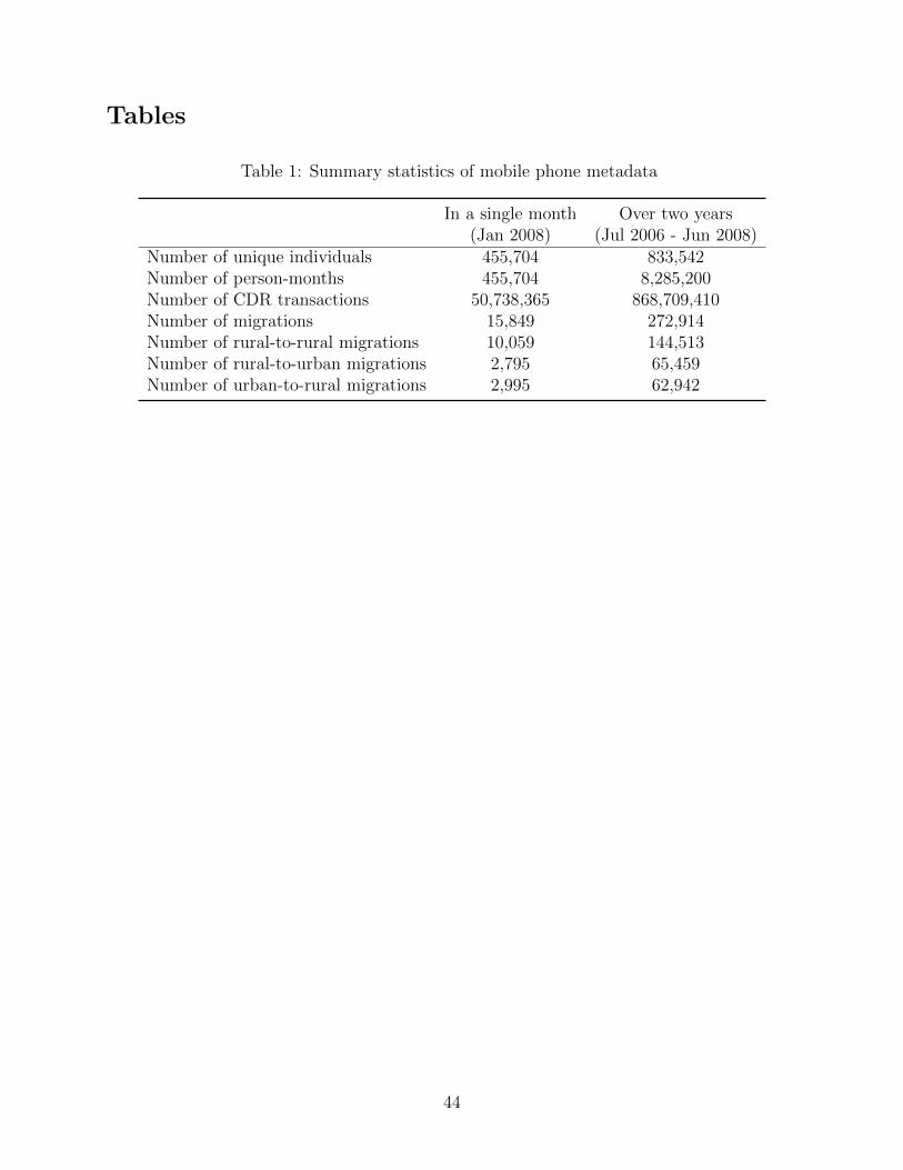
We use these data to infer migration events, and to observe the social network structure,
of each of the roughly 1.5 million unique subscribers who appear in the dataset. Summary
statistics are presented in Table 1. Our methods for inferring migration and measuring social
networks are described below. In Section 4.3, we address the fact that the mobile subscribers
we observe are a non-random sample of the overall Rwandan population, and discuss the
extent to which these issues might bias our empirical results.
3.1 Measuring migration with mobile phone metadata
We construct individual migration trajectories for each individual in three steps.
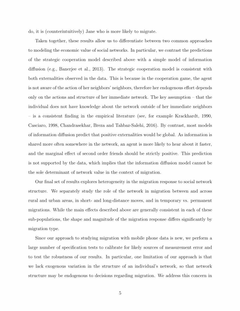
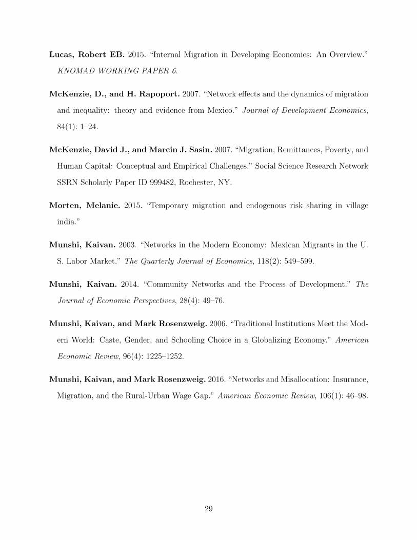
First, we extract from the CDR the approximate location of each individual at each
time in which he or she is involved in a mobile phone event, such as a phone call or text
message. This creates a set of tuples {ID, T imestamp, Location} for each subscriber. We
cannot directly observe the location of any individual in the time between events appearing
14
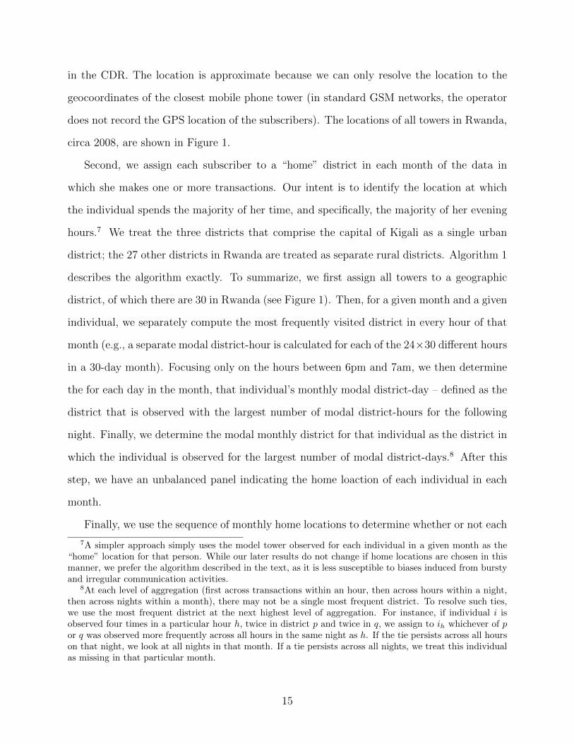
in the CDR. The location is approximate because we can only resolve the location to the
geocoordinates of the closest mobile phone tower (in standard GSM networks, the operator
does not record the GPS location of the subscribers). The locations of all towers in Rwanda,
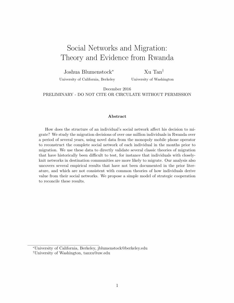
circa 2008, are shown in Figure 1.
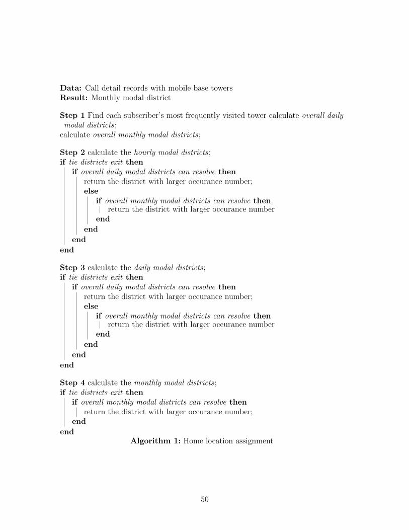
Second, we assign each subscriber to a “home” district in each month of the data in
which she makes one or more transactions. Our intent is to identify the location at which
the individual spends the majority of her time, and specifically, the majority of her evening
hours.7 We treat the three districts that comprise the capital of Kigali as a single urban
district; the 27 other districts in Rwanda are treated as separate rural districts. Algorithm 1
describes the algorithm exactly. To summarize, we first assign all towers to a geographic
district, of which there are 30 in Rwanda (see Figure 1). Then, for a given month and a given
individual, we separately compute the most frequently visited district in every hour of that
month (e.g., a separate modal district-hour is calculated for each of the 24×30 different hours
in a 30-day month). Focusing only on the hours between 6pm and 7am, we then determine
the for each day in the month, that individual’s monthly modal district-day – defined as the
district that is observed with the largest number of modal district-hours for the following
night. Finally, we determine the modal monthly district for that individual as the district in
which the individual is observed for the largest number of modal district-days.8 After this
step, we have an unbalanced panel indicating the home loaction of each individual in each
month.
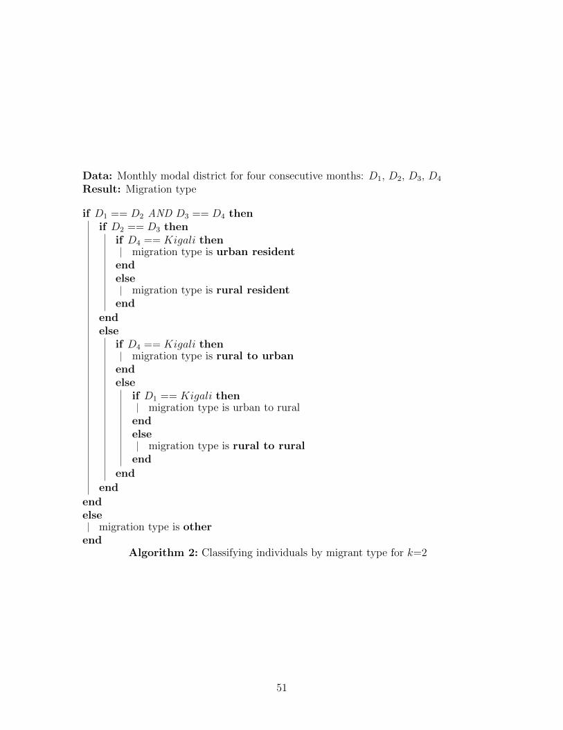
Finally, we use the sequence of monthly home locations to determine whether or not each
7A simpler approach simply uses the model tower observed for each individual in a given month as the“home” location for that person. While our later results do not change if home locations are chosen in thismanner, we prefer the algorithm described in the text, as it is less susceptible to biases induced from burstyand irregular communication activities.
8At each level of aggregation (first across transactions within an hour, then across hours within a night,then across nights within a month), there may not be a single most frequent district. To resolve such ties,we use the most frequent district at the next highest level of aggregation. For instance, if individual i isobserved four times in a particular hour h, twice in district p and twice in q, we assign to ih whichever of por q was observed more frequently across all hours in the same night as h. If the tie persists across all hourson that night, we look at all nights in that month. If a tie persists across all nights, we treat this individualas missing in that particular month.
15
individual i migrated in each month t. As in Blumenstock (2012), we say that a migration
occurs in month t if three conditions are met: (i) the individual’s home location is observed
in district d for at least k months prior to (and including) t; (ii) the home location d′ in t
is different from the home location in t + 1; and (iii) the individual’s new home location is
observed in district d′ for at least k months after (and including) t + 1. Individuals whose
home location is observed to be in d for at least k months both before and after t are
considered residents, or stayers. Individuals who do not meet these conditions are treated as
“other” (and are excluded from later analysis).9 Complete details are given in Algorithm 2.
Our preferred specifications use k = 2, i.e., we say a migration occurs if an individual stays
in one location for at least 2 months, moves to a new location, and remains in that new
location for at least 2 months. While the number of observed migrations is dependent on
the value of k chosen, we show in Section 4.2 that our results are not sensitive to reasonable
values of k.
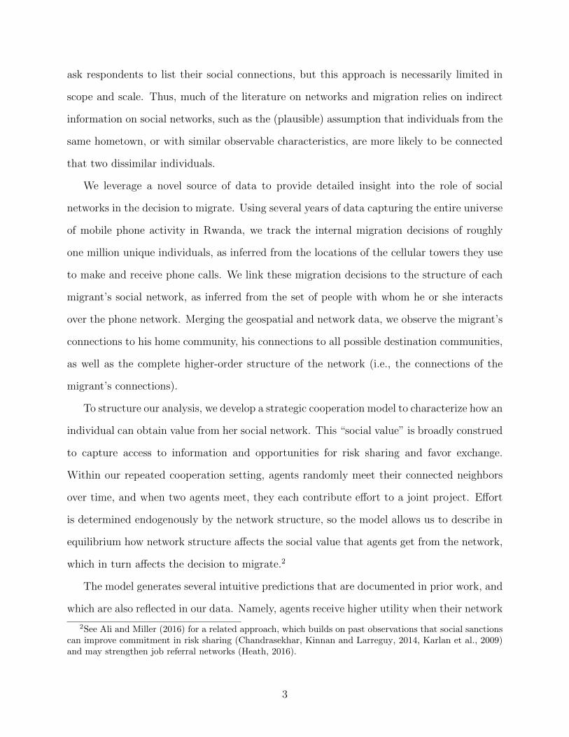
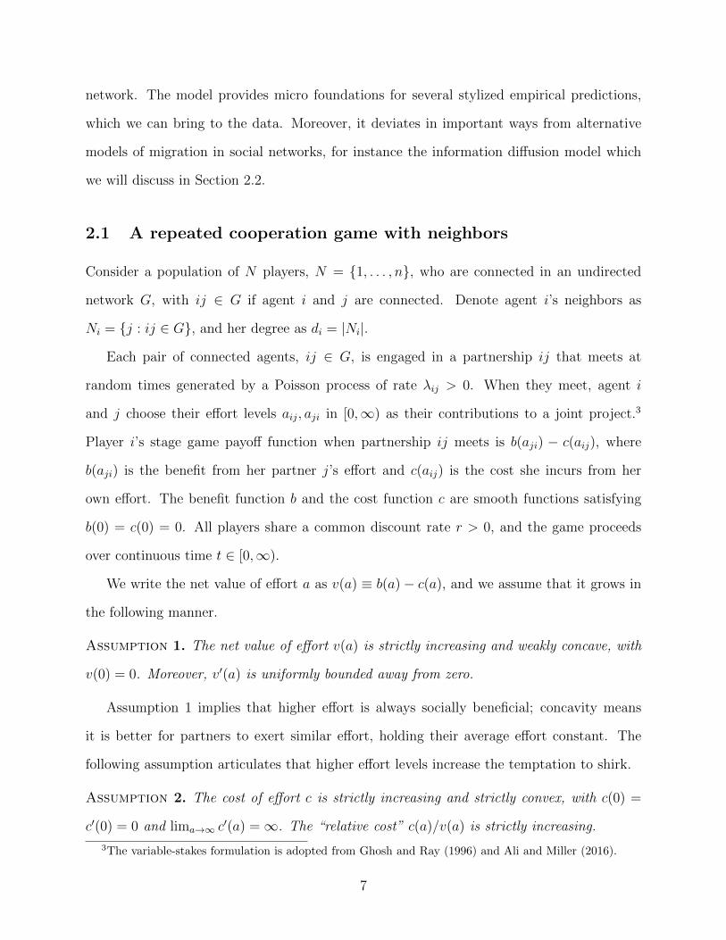
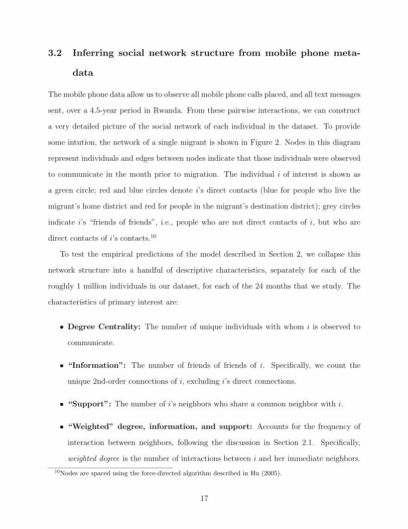
Figure 3 shows the distribution of individuals by migration status, for a single month
(January 2008). To construct this figure, and in the analysis that follows, we classify migra-
tions into three types: rural-to-urban if the individual moved from outside the capital city
of Kigali to inside Kigali; urban-to-rural if the move was from inside to outside kigali; and
rural-to-rural if the migration was between districts outside of Kigali. As can be seen in the
figure, of the 15,849 migrations observed in that month, the majority (10,059) the majority
occured between rural areas; 2,795 people moved from rural to urban areas and 2,995 moved
from urban to rural areas.
9Individuals are treated as missing in month t if they are not assigned a home location in month any ofthe months {t − k, ..., t, t + k}, for instance if they do not use their phone in that month or if there is nosingle modal district for that month. Similarly, individuals are treated as missing in t if the home locationchanges between t− k and t, or if the home location changes between t + 1 and t + k.
16
3.2 Inferring social network structure from mobile phone meta-
data
The mobile phone data allow us to observe all mobile phone calls placed, and all text messages
sent, over a 4.5-year period in Rwanda. From these pairwise interactions, we can construct
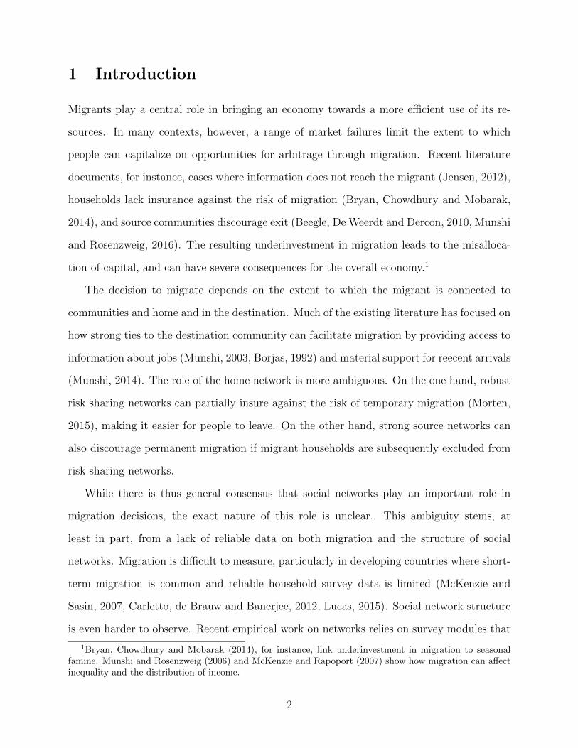
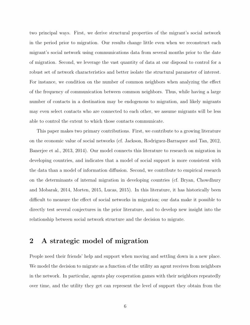
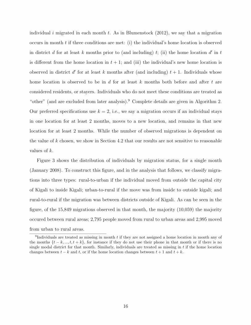
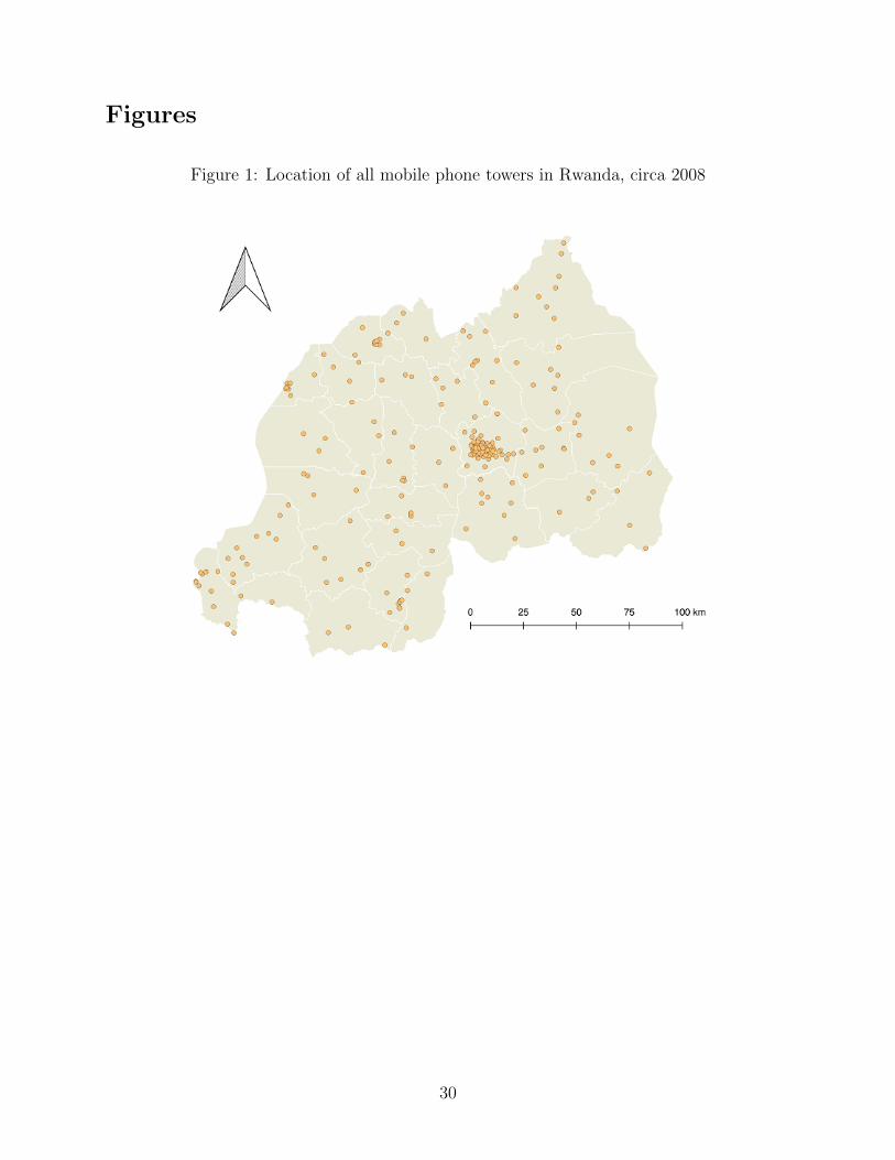
a very detailed picture of the social network of each individual in the dataset. To provide
some intution, the network of a single migrant is shown in Figure 2. Nodes in this diagram
represent individuals and edges between nodes indicate that those individuals were observed
to communicate in the month prior to migration. The individual i of interest is shown as
a green circle; red and blue circles denote i’s direct contacts (blue for people who live the
migrant’s home district and red for people in the migrant’s destination district); grey circles
indicate i’s “friends of friends”, i.e., people who are not direct contacts of i, but who are
direct contacts of i’s contacts.10
To test the empirical predictions of the model described in Section 2, we collapse this
network structure into a handful of descriptive characteristics, separately for each of the
roughly 1 million individuals in our dataset, for each of the 24 months that we study. The
characteristics of primary interest are:
• Degree Centrality: The number of unique individuals with whom i is observed to
communicate.
• “Information”: The number of friends of friends of i. Specifically, we count the
unique 2nd-order connections of i, excluding i’s direct connections.
• “Support”: The number of i’s neighbors who share a common neighbor with i.
• “Weighted” degree, information, and support: Accounts for the frequency of
interaction between neighbors, following the discussion in Section 2.1. Specifically,
weighted degree is the number of interactions between i and her immediate neighbors.
10Nodes are spaced using the force-directed algorithm described in Hu (2005).
17
weighted information is the count of all interactions between i’s neighbors and their
neighbors. Weighted support is the count of all interactions between i’s neighbors and
their common neighbors of i.
To reduce endogeneity when relating network structure to observed patterns of migration,
we compare network characteristics derived from data in month t− 1 to migration behavior
observed in month t. Concerns of serial correlation are discussed in Section 4.2
4 Estimation and Results
To study the relationship between social network structure and the decision to migrate, we
compare characteristics of individual i’s network in month t− 1 with the migration decision
made by i in month t. Our canonical specification requires that the individual remain in one
district for k = 2 months, then move to another place for k = 2 months, to be considered a
migrant. As a concrete example, when t is set to January 2008, the individual is considered
a migrant if her home location is determined to be one district d in December 2007 and
January 2008, and a different district d′ 6= d in both February 2008 and March 2008. The
first column of Table 1 shows how the sample of XXX unique individuals is distributed
across residents and migrants, for just the month of January 2008. To increase the power of
our analysis, we then aggregate migration behavior over the 24 months between July 2006
and June 2008. Summary statistics for this aggregated person-month dataset are given in
Table 1, column 2.11
We calculate properties of i’s network in t − 1 following the procedures described in
Section 3.2 for both the individual’s home and destination networks. This is a straightforward
process for the home network: we determine i’s home location d in t−1, consider all contacts
of i whose home location in t − 1 was also d, and then calculate the properties of that
11Note that this process of aggregation means that a single individual will appear multiple times in ouranalysis. While this was our intent, since repeat migration is quite common in Rwanda, in later robustnesstests we show that very little changes if we restrict our analysis to a single month.
18
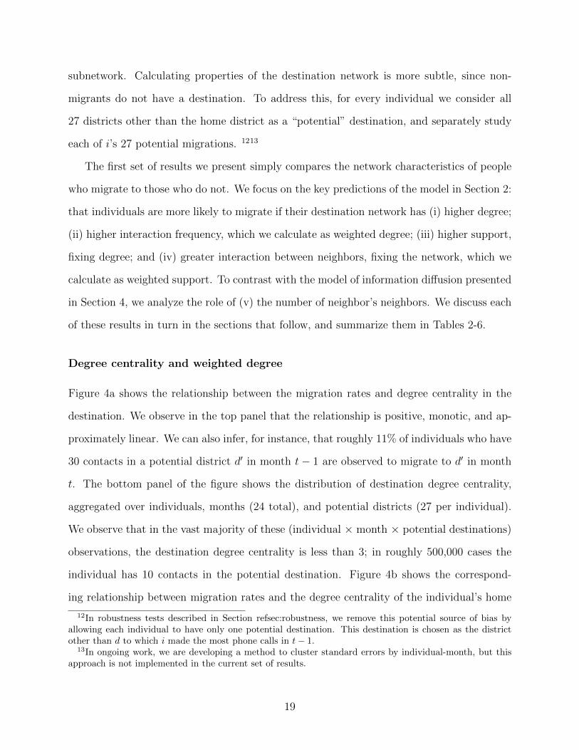
subnetwork. Calculating properties of the destination network is more subtle, since non-
migrants do not have a destination. To address this, for every individual we consider all
27 districts other than the home district as a “potential” destination, and separately study
each of i’s 27 potential migrations. 1213
The first set of results we present simply compares the network characteristics of people
who migrate to those who do not. We focus on the key predictions of the model in Section 2:
that individuals are more likely to migrate if their destination network has (i) higher degree;
(ii) higher interaction frequency, which we calculate as weighted degree; (iii) higher support,
fixing degree; and (iv) greater interaction between neighbors, fixing the network, which we
calculate as weighted support. To contrast with the model of information diffusion presented
in Section 4, we analyze the role of (v) the number of neighbor’s neighbors. We discuss each
of these results in turn in the sections that follow, and summarize them in Tables 2-6.
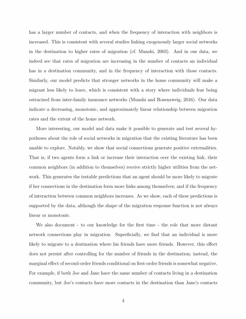
Degree centrality and weighted degree
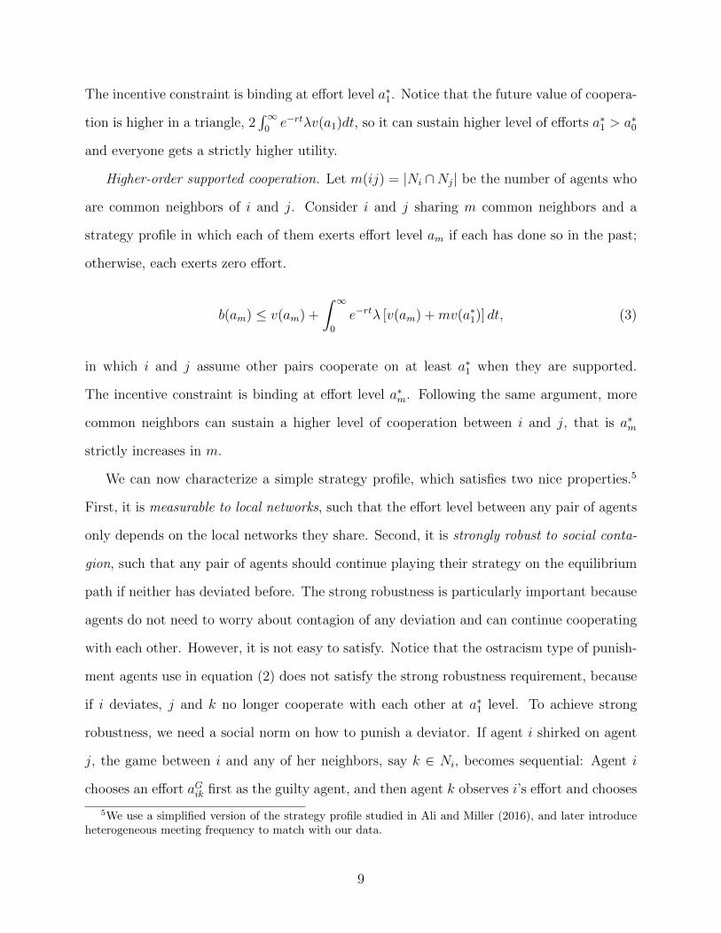
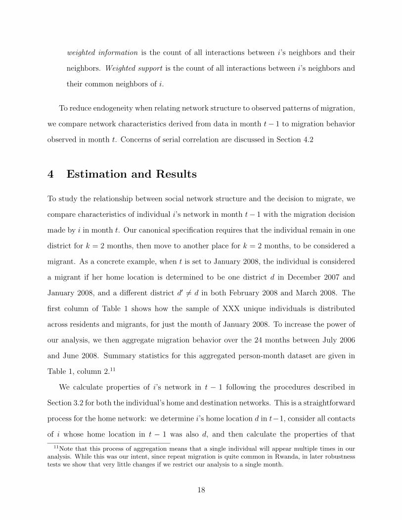
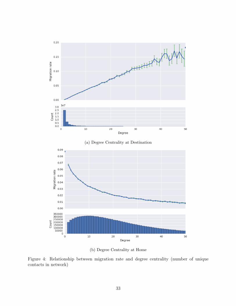
Figure 4a shows the relationship between the migration rates and degree centrality in the
destination. We observe in the top panel that the relationship is positive, monotic, and ap-
proximately linear. We can also infer, for instance, that roughly 11% of individuals who have
30 contacts in a potential district d′ in month t− 1 are observed to migrate to d′ in month
t. The bottom panel of the figure shows the distribution of destination degree centrality,
aggregated over individuals, months (24 total), and potential districts (27 per individual).
We observe that in the vast majority of these (individual × month × potential destinations)
observations, the destination degree centrality is less than 3; in roughly 500,000 cases the
individual has 10 contacts in the potential destination. Figure 4b shows the correspond-
ing relationship between migration rates and the degree centrality of the individual’s home
12In robustness tests described in Section refsec:robustness, we remove this potential source of bias byallowing each individual to have only one potential destination. This destination is chosen as the districtother than d to which i made the most phone calls in t− 1.
13In ongoing work, we are developing a method to cluster standard errors by individual-month, but thisapproach is not implemented in the current set of results.
19
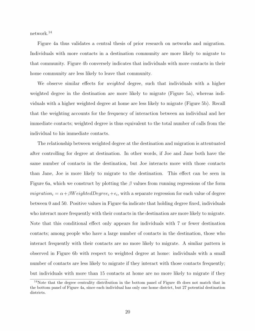
network.14
Figure 4a thus validates a central thesis of prior research on networks and migration.
Individuals with more contacts in a destination community are more likely to migrate to
that community. Figure 4b conversely indicates that individuals with more contacts in their
home community are less likely to leave that community.
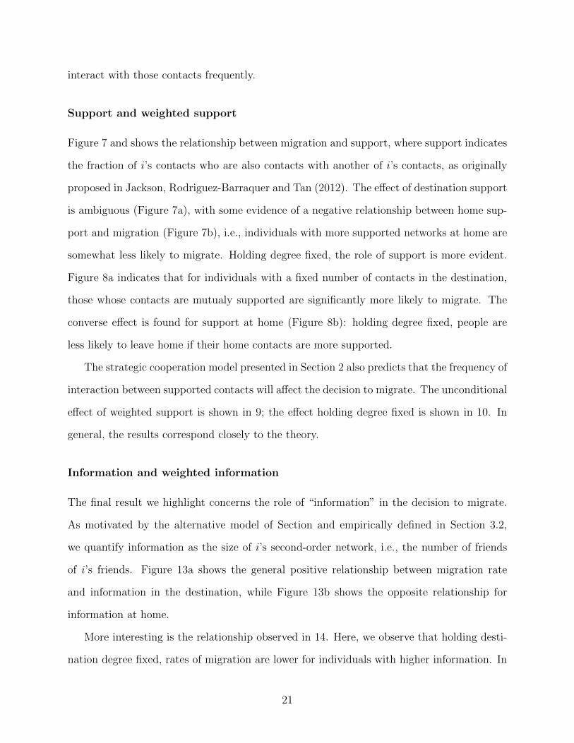
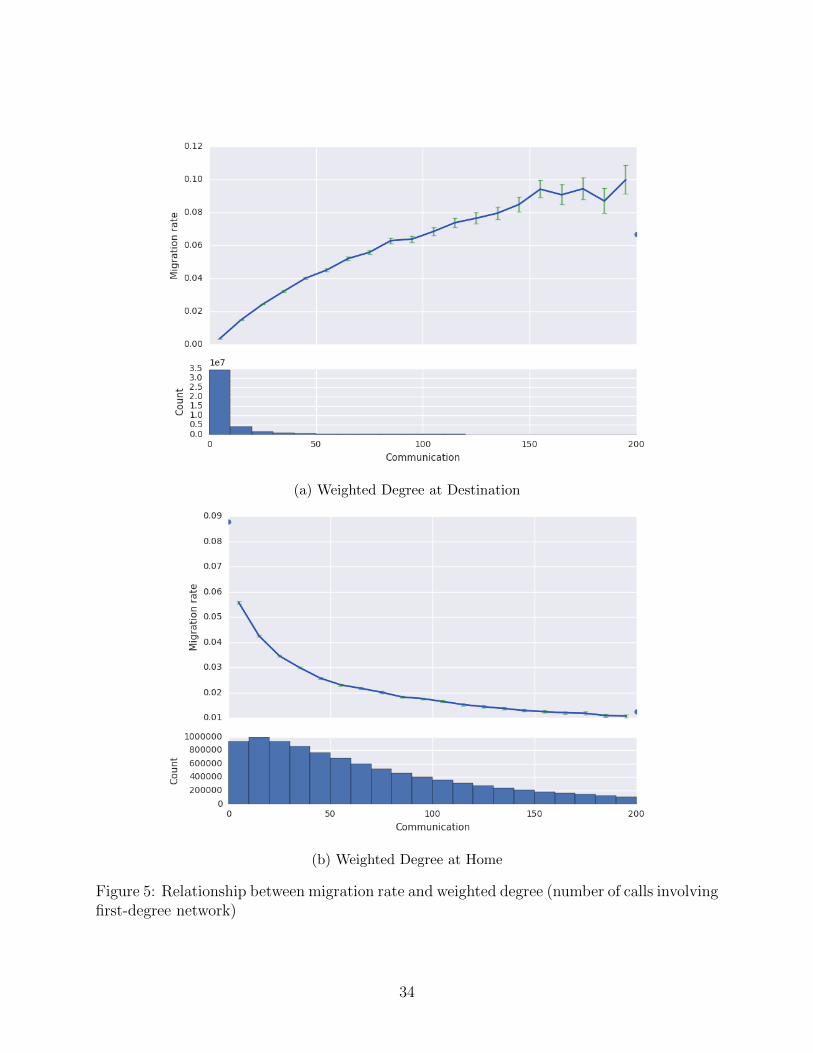
We observe similar effects for weighted degree, such that individuals with a higher
weighted degree in the destination are more likely to migrate (Figure 5a), whereas indi-
viduals with a higher weighted degree at home are less likely to migrate (Figure 5b). Recall
that the weighting accounts for the frequency of interaction between an individual and her
immediate contacts; weighted degree is thus equivalent to the total number of calls from the
individual to his immediate contacts.
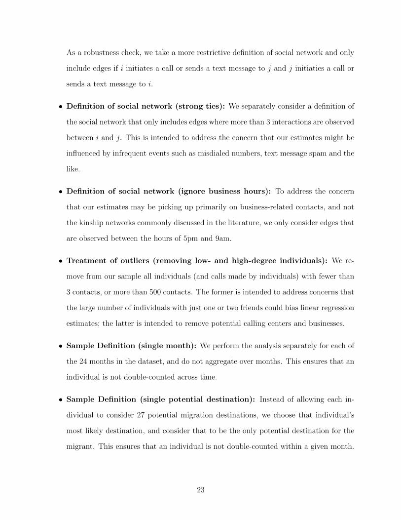
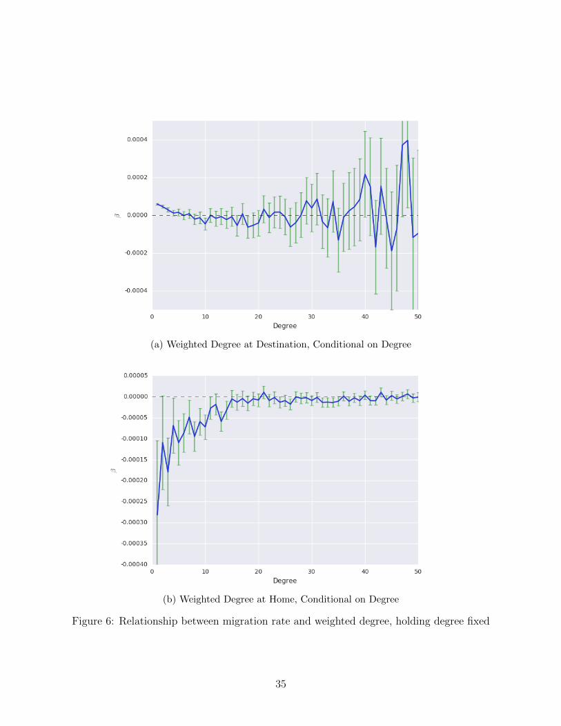
The relationship between weighted degree at the destination and migration is attentuated
after controlling for degree at destination. In other words, if Joe and Jane both have the
same number of contacts in the destination, but Joe interacts more with those contacts
than Jane, Joe is more likely to migrate to the destination. This effect can be seen in
Figure 6a, which we construct by plotting the β values from running regressions of the form
migrationi = α+βWeightedDegreei+εi, with a separate regression for each value of degree
between 0 and 50. Positive values in Figure 6a indicate that holding degree fixed, individuals
who interact more frequently with their contacts in the destination are more likely to migrate.
Note that this conditional effect only appears for individuals with 7 or fewer destination
contacts; among people who have a large number of contacts in the destination, those who
interact frequently with their contacts are no more likely to migrate. A simliar pattern is
observed in Figure 6b with respect to weighted degree at home: individuals with a small
number of contacts are less likely to migrate if they interact with those contacts frequently;
but individuals with more than 15 contacts at home are no more likely to migrate if they
14Note that the degree centrality distribution in the bottom panel of Figure 4b does not match that inthe bottom panel of Figure 4a, since each individual has only one home district, but 27 potential destinationdistricts.
20
interact with those contacts frequently.
Support and weighted support
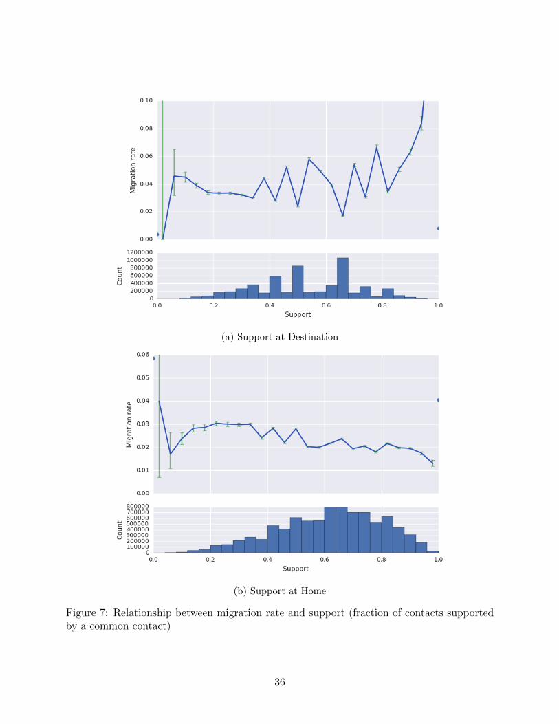
Figure 7 and shows the relationship between migration and support, where support indicates
the fraction of i’s contacts who are also contacts with another of i’s contacts, as originally
proposed in Jackson, Rodriguez-Barraquer and Tan (2012). The effect of destination support
is ambiguous (Figure 7a), with some evidence of a negative relationship between home sup-
port and migration (Figure 7b), i.e., individuals with more supported networks at home are
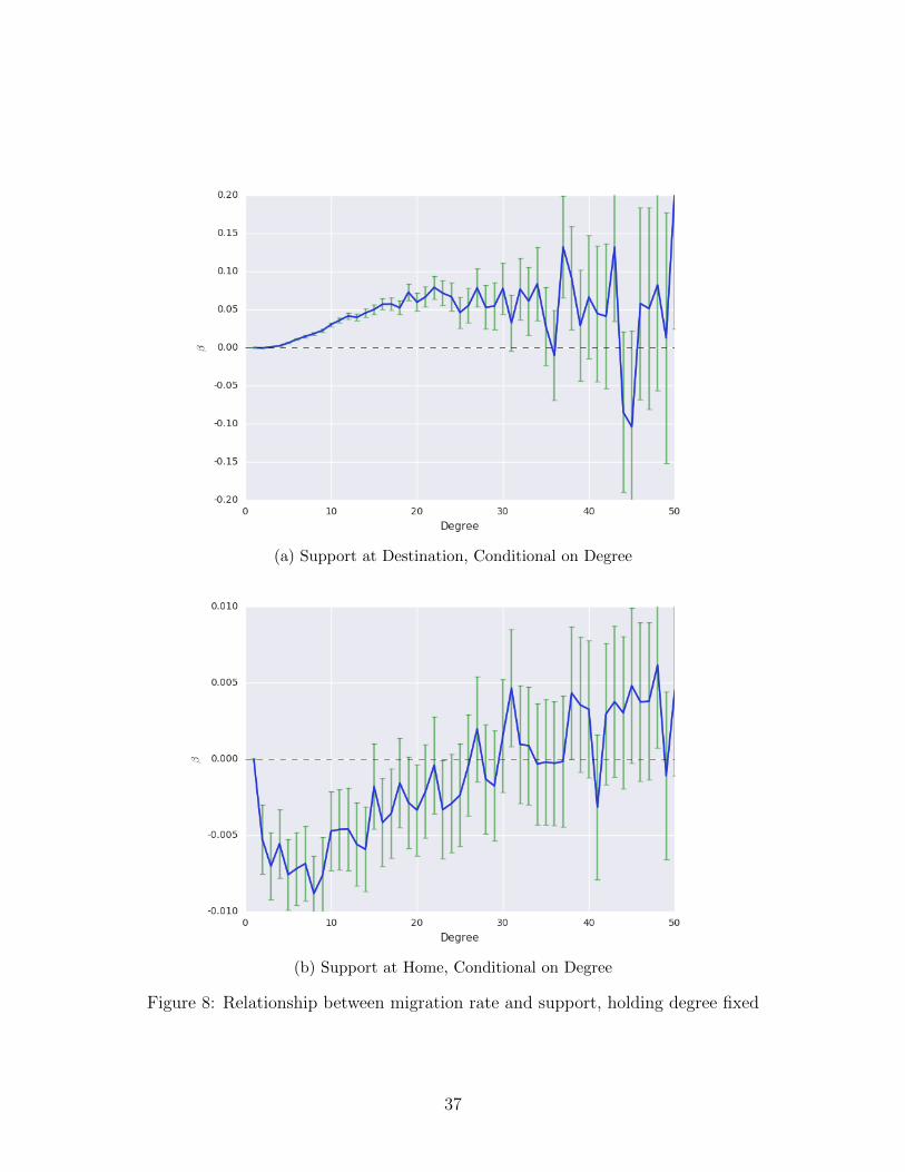
somewhat less likely to migrate. Holding degree fixed, the role of support is more evident.
Figure 8a indicates that for individuals with a fixed number of contacts in the destination,
those whose contacts are mutualy supported are significantly more likely to migrate. The
converse effect is found for support at home (Figure 8b): holding degree fixed, people are
less likely to leave home if their home contacts are more supported.
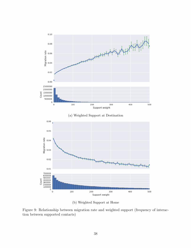
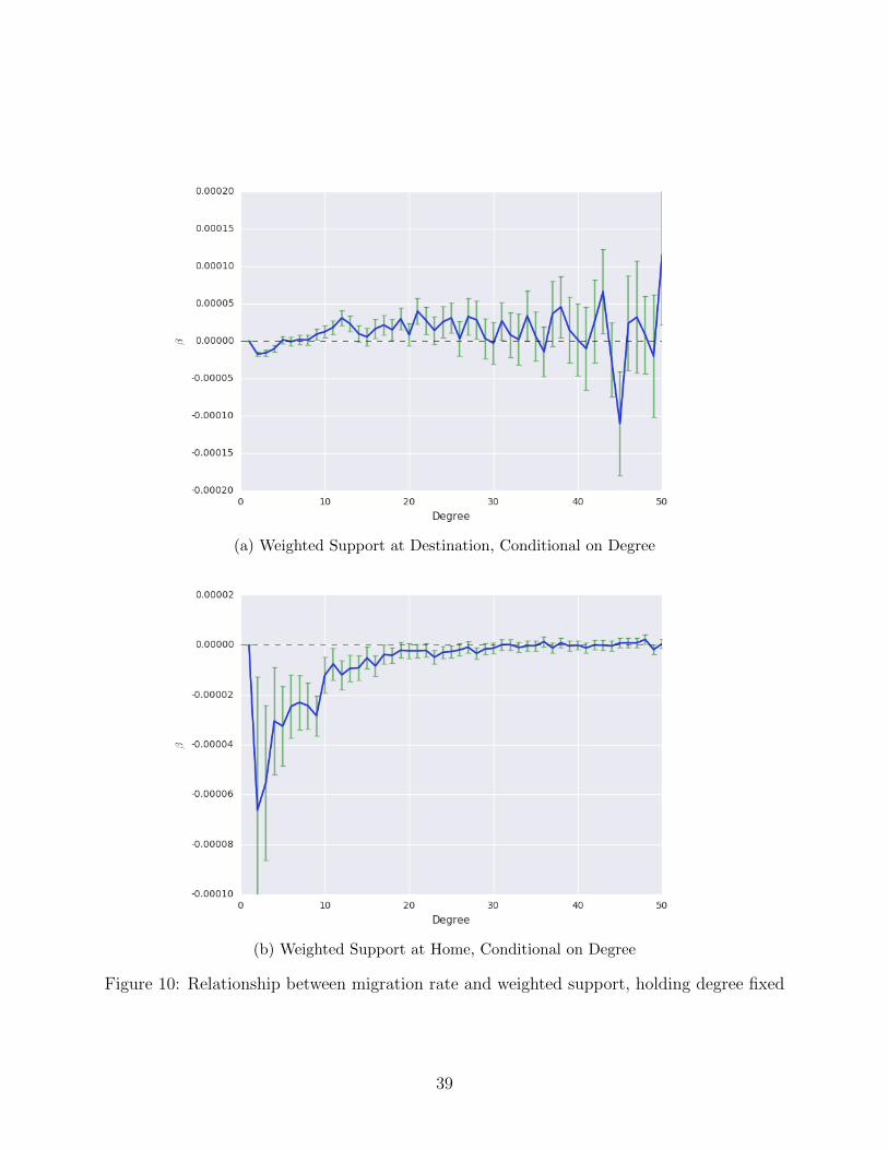
The strategic cooperation model presented in Section 2 also predicts that the frequency of
interaction between supported contacts will affect the decision to migrate. The unconditional
effect of weighted support is shown in 9; the effect holding degree fixed is shown in 10. In
general, the results correspond closely to the theory.
Information and weighted information
The final result we highlight concerns the role of “information” in the decision to migrate.
As motivated by the alternative model of Section and empirically defined in Section 3.2,
we quantify information as the size of i’s second-order network, i.e., the number of friends
of i’s friends. Figure 13a shows the general positive relationship between migration rate
and information in the destination, while Figure 13b shows the opposite relationship for
information at home.
More interesting is the relationship observed in 14. Here, we observe that holding desti-
nation degree fixed, rates of migration are lower for individuals with higher information. In
21

other words, if both Joe and Jane have the same number of contacts living in a destination
community, but Joe’s contacts have more contacts in the destination than Jane’s contacts
do, it is Jane who is more likely to migrate.
4.1 Heterogeneity
[This section under revision, contact authors for details]
Urban and rural migrants
Temporary and permanent migration
Strong and weak ties
4.2 Robustness
The empirical results described above are robust to a large number of alternative specifica-
tions. In results available upon request, we have verified that our results are not affected by
any of the following:
• How we define “migration” (choice of k): Our main specifications set k = 2, i.e.,
we say an individual has migrated if she spends 2 or more months in d and then 2 or
more months in d′ 6= d. We observe qualitatively similar results for k = 1 and k = 3.
• How we define “migration” (home location sensitivity): Our assignment of
individuals to home locations is based on the set of mobile phone towers through
wihch their communication is routed. Since there is a degree of noise in this process,
we take a more restrictive definition of migration that only considers migrants that
move between non-adjacent districts.
• Definition of social network (reciprocated edges): In constructing the social
network from the mobile phone data, we normally consider an edge to exist between i
and j if we observe one or more phone call or text message between these individuals.
22
As a robustness check, we take a more restrictive definition of social network and only
include edges if i initiates a call or sends a text message to j and j initiaties a call or
sends a text message to i.
• Definition of social network (strong ties): We separately consider a definition of
the social network that only includes edges where more than 3 interactions are observed
between i and j. This is intended to address the concern that our estimates might be
influenced by infrequent events such as misdialed numbers, text message spam and the
like.
• Definition of social network (ignore business hours): To address the concern
that our estimates may be picking up primarily on business-related contacts, and not
the kinship networks commonly discussed in the literature, we only consider edges that
are observed between the hours of 5pm and 9am.
• Treatment of outliers (removing low- and high-degree individuals): We re-
move from our sample all individuals (and calls made by individuals) with fewer than
3 contacts, or more than 500 contacts. The former is intended to address concerns that
the large number of individuals with just one or two friends could bias linear regression
estimates; the latter is intended to remove potential calling centers and businesses.
• Sample Definition (single month): We perform the analysis separately for each of
the 24 months in the dataset, and do not aggregate over months. This ensures that an
individual is not double-counted across time.
• Sample Definition (single potential destination): Instead of allowing each in-
dividual to consider 27 potential migration destinations, we choose that individual’s
most likely destination, and consider that to be the only potential destination for the
migrant. This ensures that an individual is not double-counted within a given month.
23
4.3 Population representativeness and external validity
Our data allow us to observe the movement patterns and social network structures of a large
population of mobile phone owners in Rwanda. These mobile subscribers represent a non-
random subset of the overall Rwandan population. Likewise, the social network connections
we observe for any given subscriber are assumed to be a partial and non-random subset of
that subscriber’s true social network.15
5 Discussion
The key empirical results are summarized in Tables 2-6. In short, we observe that (i) migra-
tion rates increase when individuals have a greater number of contacts in the destination,
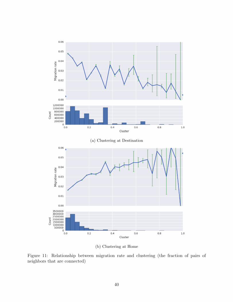
and when they interact with those contacts more frequently; (ii) that positive externalities
exist, such that migration rates are higher when destination networks provide higher support
and clustering, and when the strength of supported links is greater; (iii) that these external-
ities are local, in the sense that individuals are not more likely to migrate to a place where
they have more friends of friends, if the number of direct friends is held constant. Roughly
opposite effects are found with respect to the structure of the home network: people are less
likely to leave when their home network is larger and denser - with the prominent exception
that the externalities are global at home.
Taken together, this evidence is largely consistent with a model of strategic cooperation
in which agents observe limited information about their network, beyond their immediate
neighbors. It is harder to reconcile these results with a model of mechanical information
diffusion model. However, the strategic information diffusion model can be built upon our
main model. Specifically, if agents can strategically choose with whom they communicate
and the level of effort to invest in communication – i.e., they can increase the probability p –
then agents are more likely to share the information with their neighbors, who are currently
15This section is under revision, contact authors for details.
24
in a different location and with whom they share a tighter local network and expect a higher
utility from future cooperation.16
6 Conclusion
This paper presents new theory and evidence on the role that social network play in the
decision to migrate. Our approach highlights how new sources of large-scale digital data
can be used to simultaneously observe migration histories and the dynamic structure of
social networks at a level of detail and scale that has not been achieved in prior work.
These data make it possible to directly validate several long-standing assumptions in the
literature on migration, which have been hard to test with traditional sources of data. For
instance, we show that individuals are more likely to migrate to destinations where they
have a large number of contacts, and that the elasticity of this response is approximately
one (e.g., someone with 20 contacts in the destination is roughly twice as likely to migrate
as someone with 10 contacts).
We also document several novel properties of the relationship between social networks
and migration, not all which can be explained by canonical models of information diffusion.
For instance, we find that migration rates are not positively correlated with the number of
friends of friends that one has in the destination, but that the migration rate is negatively
correlated with the number of friends of friends at home. To reconcile these results, we
propose a model of strategic cooperation that characterizes how individuals obtain value
from their social network, and which fits the data quite well.
There are several directions to extend our analysis. First, while we focus on how social
network affects migration decision, migration could also change the network structure. For
example, condition on one agent will migration or has just migrated, we can examine how he
forms new links and deletes existing ones. Also, the ability to observe migration over several
16For example, Banerjee et al. (2013) find that agents who themselves participate in microfinance informa given neighbor about this program with probability 45%, while others inform a given neighbor withprobability 9.5%.
25

years could allow us to study migration cascade, and its relationship with the home network.
For example, if the home network is sparse, migration cascade may not happen because the
contagion is too weak; if the home network is very dense, migration cascade also may not
happen because the risk-sharing at home could hold people from moving.
26
References
Ali, S. Nageeb, and David A. Miller. 2016. “Ostracism and Forgiveness.” American
Economic Review, 106(8): 2329–2348.
Banerjee, Abhijit, Arun G. Chandrasekhar, Esther Duflo, and Matthew O. Jack-
son. 2013. “The Diffusion of Microfinance.” Science, 341(6144): 1236498.
Banerjee, Abhijit, Arun G. Chandrasekhar, Esther Duflo, and Matthew O. Jack-
son. 2014. “Gossip: Identifying Central Individuals in a Social Network.” National Bureau
of Economic Research Working Paper 20422.
Beegle, Kathleen, Joachim De Weerdt, and Stefan Dercon. 2010. “Migration and
Economic Mobility in Tanzania: Evidence from a Tracking Survey.” Review of Economics
and Statistics, 93(3): 1010–1033.
Blumenstock, Joshua Evan. 2012. “Inferring Patterns of Internal Migration from Mobile
Phone Call Records: Evidence from Rwanda.” Information Technology for Development,
18(2): 107–125.
Borjas, George J. 1992. “Ethnic Capital and Intergenerational Mobility.” The Quarterly
Journal of Economics, 107(1): 123–150.
Bryan, Gharad, Shyamal Chowdhury, and Ahmed Mushfiq Mobarak. 2014. “Un-
derinvestment in a Profitable Technology: The Case of Seasonal Migration in Bangladesh.”
Econometrica, 82(5): 1671–1748.
Carletto, Calogero, Alan de Brauw, and Raka Banerjee. 2012. “Measuring migration
in multi-topic household surveys.” Handbook of Research Methods in Migration, 207.
Casciaro, Tiziana. 1998. “Seeing things clearly: social structure, personality, and accuracy
in social network perception.” Social Networks, 20(4): 331–351.
27
Chandrasekhar, Arun, Emily Breza, and Alireza Tahbaz-Salehi. 2016. “Seeing the
forest for the trees? an investigation of network knowledge.” Working Paper.
Chandrasekhar, Arun G., Cynthia Kinnan, and Horacio Larreguy. 2014. “Social
networks as contract enforcement: Evidence from a lab experiment in the field.” National
Bureau of Economic Research.
Ghosh, Parikshit, and Debraj Ray. 1996. “Cooperation in Community Interaction With-
out Information Flows.” The Review of Economic Studies, 63(3): 491–519.
Heath, Rachel. 2016. “Why do firms hire using referrals? Evidence from Bangladeshi
Garment Factories.”
Hu, Yifan. 2005. “Efficient, high-quality force-directed graph drawing.” Mathematica Jour-
nal, 10(1): 37–71.
Jackson, Matthew O., and Leeat Yariv. 2010. “Diffusion, strategic interaction, and
social structure.” Handbook of Social Economics, edited by J. Benhabib, A. Bisin and M.
Jackson.
Jackson, Matthew O., Tomas Rodriguez-Barraquer, and Xu Tan. 2012. “Social
capital and social quilts: Network patterns of favor exchange.” The American Economic
Review, 102(5): 1857–1897.
Jensen, Robert. 2012. “Do Labor Market Opportunities Affect Young Women’s Work
and Family Decisions? Experimental Evidence from India.” The Quarterly Journal of
Economics, 127(2): 753–792.
Karlan, Dean, Markus Mobius, Tanya Rosenblat, and Adam Szeidl. 2009. “Trust
and Social Collateral.” The Quarterly Journal of Economics, 124(3): 1307 –1361.
Krackhardt, David. 1990. “Assessing the political landscape: Structure, cognition, and
power in organizations.” Administrative science quarterly, 342–369.
28
Lucas, Robert EB. 2015. “Internal Migration in Developing Economies: An Overview.”
KNOMAD WORKING PAPER 6.
McKenzie, D., and H. Rapoport. 2007. “Network effects and the dynamics of migration
and inequality: theory and evidence from Mexico.” Journal of Development Economics,
84(1): 1–24.
McKenzie, David J., and Marcin J. Sasin. 2007. “Migration, Remittances, Poverty, and
Human Capital: Conceptual and Empirical Challenges.” Social Science Research Network
SSRN Scholarly Paper ID 999482, Rochester, NY.
Morten, Melanie. 2015. “Temporary migration and endogenous risk sharing in village
india.”
Munshi, Kaivan. 2003. “Networks in the Modern Economy: Mexican Migrants in the U.
S. Labor Market.” The Quarterly Journal of Economics, 118(2): 549–599.
Munshi, Kaivan. 2014. “Community Networks and the Process of Development.” The
Journal of Economic Perspectives, 28(4): 49–76.
Munshi, Kaivan, and Mark Rosenzweig. 2006. “Traditional Institutions Meet the Mod-
ern World: Caste, Gender, and Schooling Choice in a Globalizing Economy.” American
Economic Review, 96(4): 1225–1252.
Munshi, Kaivan, and Mark Rosenzweig. 2016. “Networks and Misallocation: Insurance,
Migration, and the Rural-Urban Wage Gap.” American Economic Review, 106(1): 46–98.
29
Figures
Figure 1: Location of all mobile phone towers in Rwanda, circa 2008
30
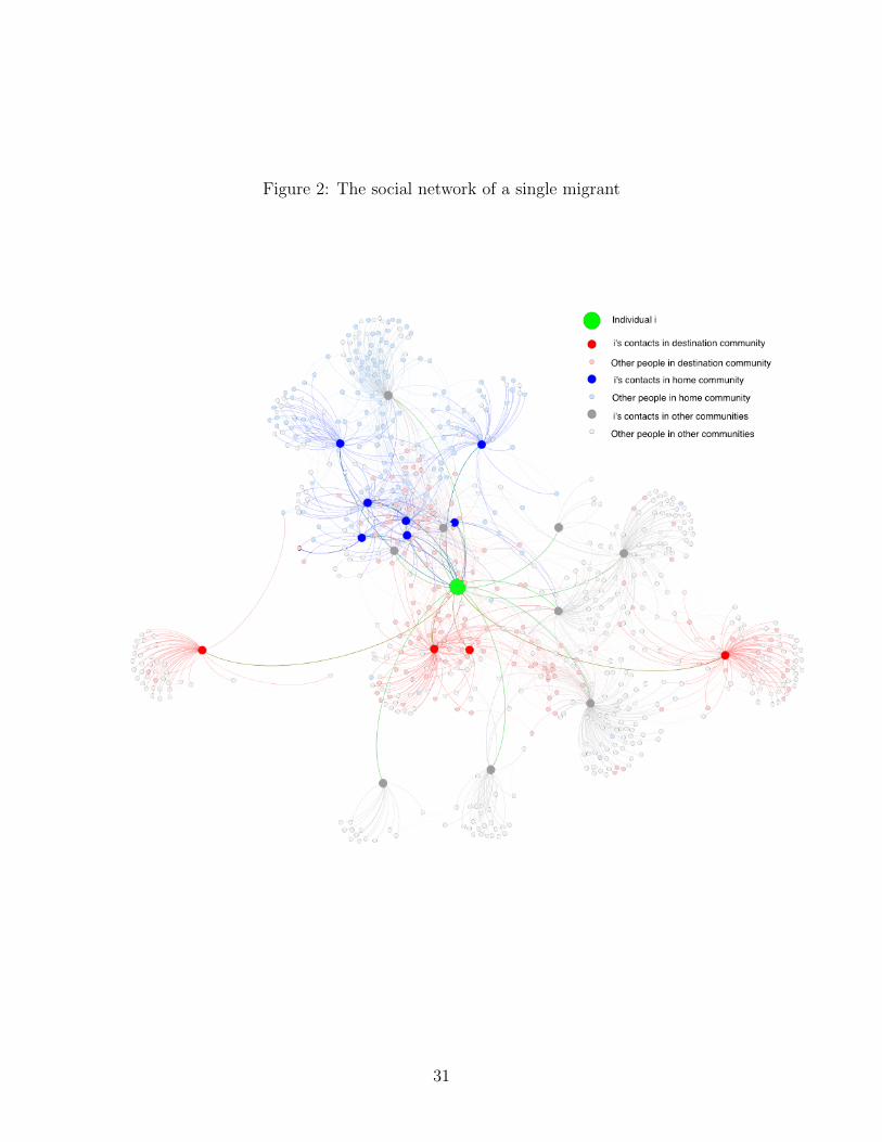
Figure 2: The social network of a single migrant
31
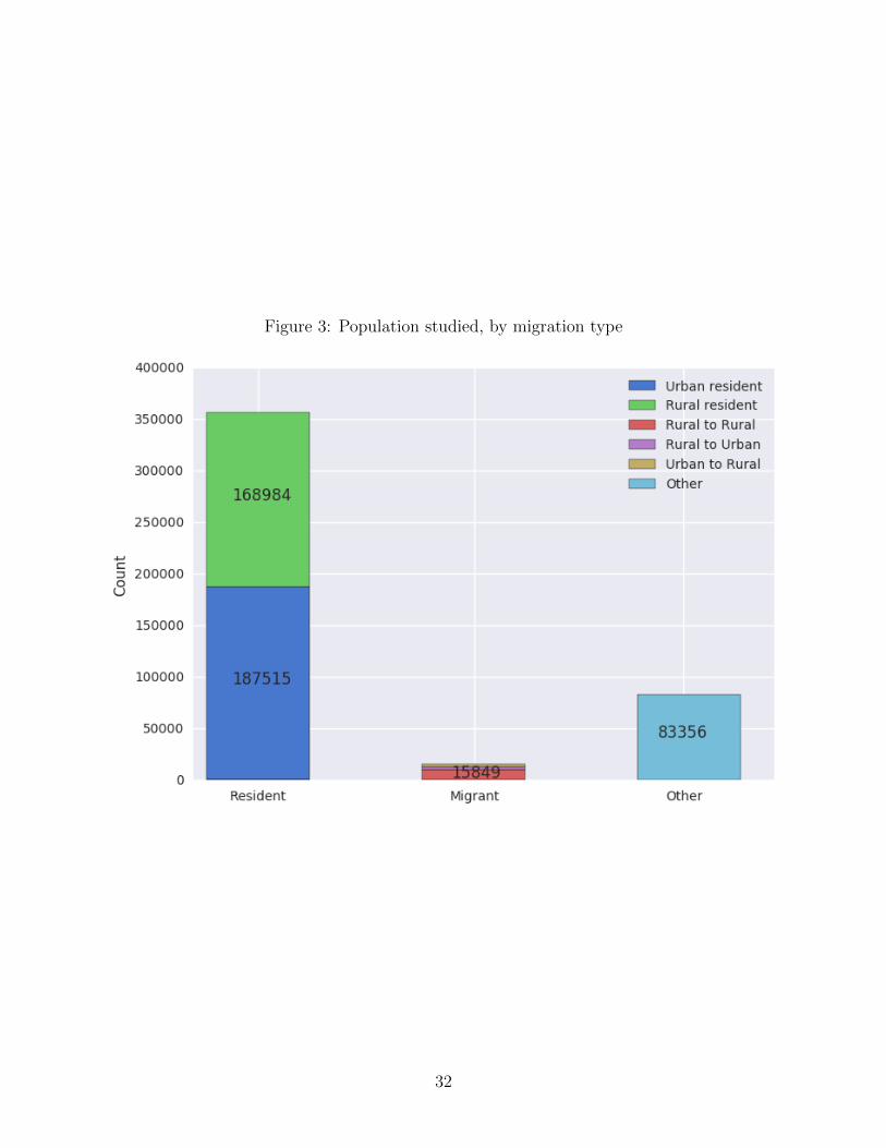
Figure 3: Population studied, by migration type
32
(a) Degree Centrality at Destination
(b) Degree Centrality at Home
Figure 4: Relationship between migration rate and degree centrality (number of uniquecontacts in network)
33
(a) Weighted Degree at Destination
(b) Weighted Degree at Home
Figure 5: Relationship between migration rate and weighted degree (number of calls involvingfirst-degree network)
34
(a) Weighted Degree at Destination, Conditional on Degree
(b) Weighted Degree at Home, Conditional on Degree
Figure 6: Relationship between migration rate and weighted degree, holding degree fixed
35
(a) Support at Destination
(b) Support at Home
Figure 7: Relationship between migration rate and support (fraction of contacts supportedby a common contact)
36
(a) Support at Destination, Conditional on Degree
(b) Support at Home, Conditional on Degree
Figure 8: Relationship between migration rate and support, holding degree fixed
37
(a) Weighted Support at Destination
(b) Weighted Support at Home
Figure 9: Relationship between migration rate and weighted support (frequency of interac-tion between supported contacts)
38
(a) Weighted Support at Destination, Conditional on Degree
(b) Weighted Support at Home, Conditional on Degree
Figure 10: Relationship between migration rate and weighted support, holding degree fixed
39
(a) Clustering at Destination
(b) Clustering at Home
Figure 11: Relationship between migration rate and clustering (the fraction of pairs ofneighbors that are connected)
40
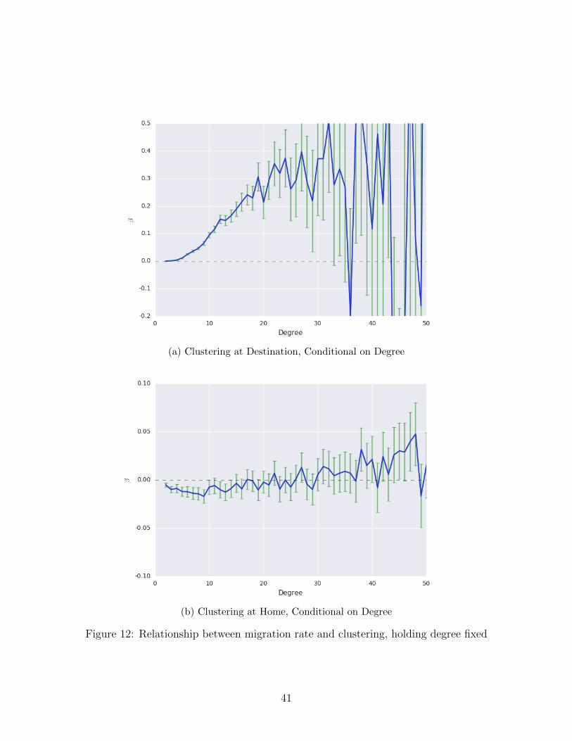
(a) Clustering at Destination, Conditional on Degree
(b) Clustering at Home, Conditional on Degree
Figure 12: Relationship between migration rate and clustering, holding degree fixed
41
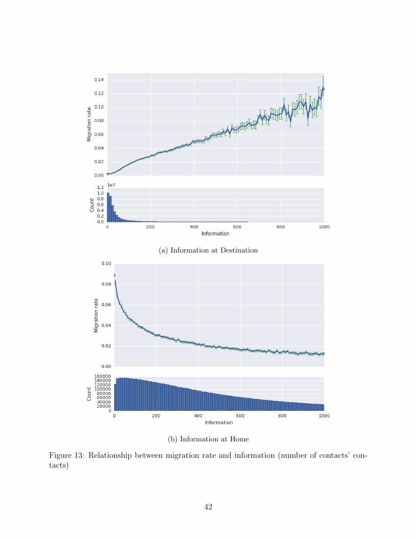
(a) Information at Destination
(b) Information at Home
Figure 13: Relationship between migration rate and information (number of contacts’ con-tacts)
42
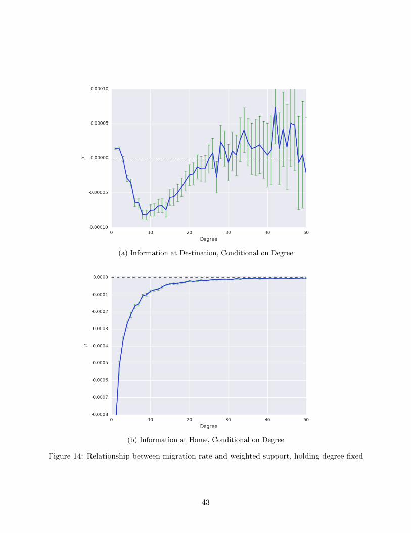
(a) Information at Destination, Conditional on Degree
(b) Information at Home, Conditional on Degree
Figure 14: Relationship between migration rate and weighted support, holding degree fixed
43
Tables
Table 1: Summary statistics of mobile phone metadata
In a single month Over two years(Jan 2008) (Jul 2006 - Jun 2008)
Number of unique individuals 455,704 833,542Number of person-months 455,704 8,285,200Number of CDR transactions 50,738,365 868,709,410Number of migrations 15,849 272,914Number of rural-to-rural migrations 10,059 144,513Number of rural-to-urban migrations 2,795 65,459Number of urban-to-rural migrations 2,995 62,942
44
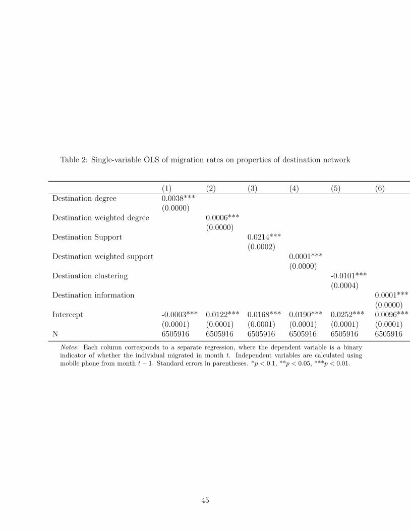
Table 2: Single-variable OLS of migration rates on properties of destination network
(1) (2) (3) (4) (5) (6)Destination degree 0.0038***
(0.0000)Destination weighted degree 0.0006***
(0.0000)Destination Support 0.0214***
(0.0002)Destination weighted support 0.0001***
(0.0000)Destination clustering -0.0101***
(0.0004)Destination information 0.0001***
(0.0000)Intercept -0.0003*** 0.0122*** 0.0168*** 0.0190*** 0.0252*** 0.0096***
(0.0001) (0.0001) (0.0001) (0.0001) (0.0001) (0.0001)N 6505916 6505916 6505916 6505916 6505916 6505916
Notes: Each column corresponds to a separate regression, where the dependent variable is a binaryindicator of whether the individual migrated in month t. Independent variables are calculated usingmobile phone from month t− 1. Standard errors in parentheses. *p < 0.1, **p < 0.05, ***p < 0.01.
45
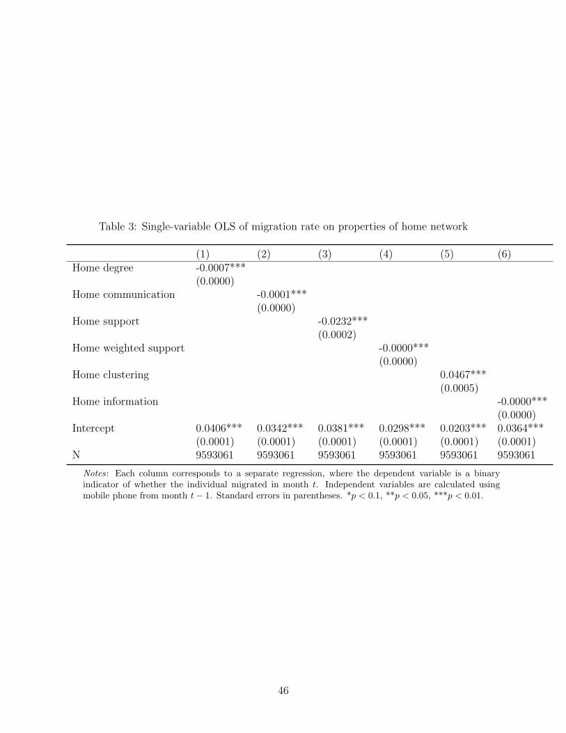
Table 3: Single-variable OLS of migration rate on properties of home network
(1) (2) (3) (4) (5) (6)Home degree -0.0007***
(0.0000)Home communication -0.0001***
(0.0000)Home support -0.0232***
(0.0002)Home weighted support -0.0000***
(0.0000)Home clustering 0.0467***
(0.0005)Home information -0.0000***
(0.0000)Intercept 0.0406*** 0.0342*** 0.0381*** 0.0298*** 0.0203*** 0.0364***
(0.0001) (0.0001) (0.0001) (0.0001) (0.0001) (0.0001)N 9593061 9593061 9593061 9593061 9593061 9593061
Notes: Each column corresponds to a separate regression, where the dependent variable is a binaryindicator of whether the individual migrated in month t. Independent variables are calculated usingmobile phone from month t− 1. Standard errors in parentheses. *p < 0.1, **p < 0.05, ***p < 0.01.
46
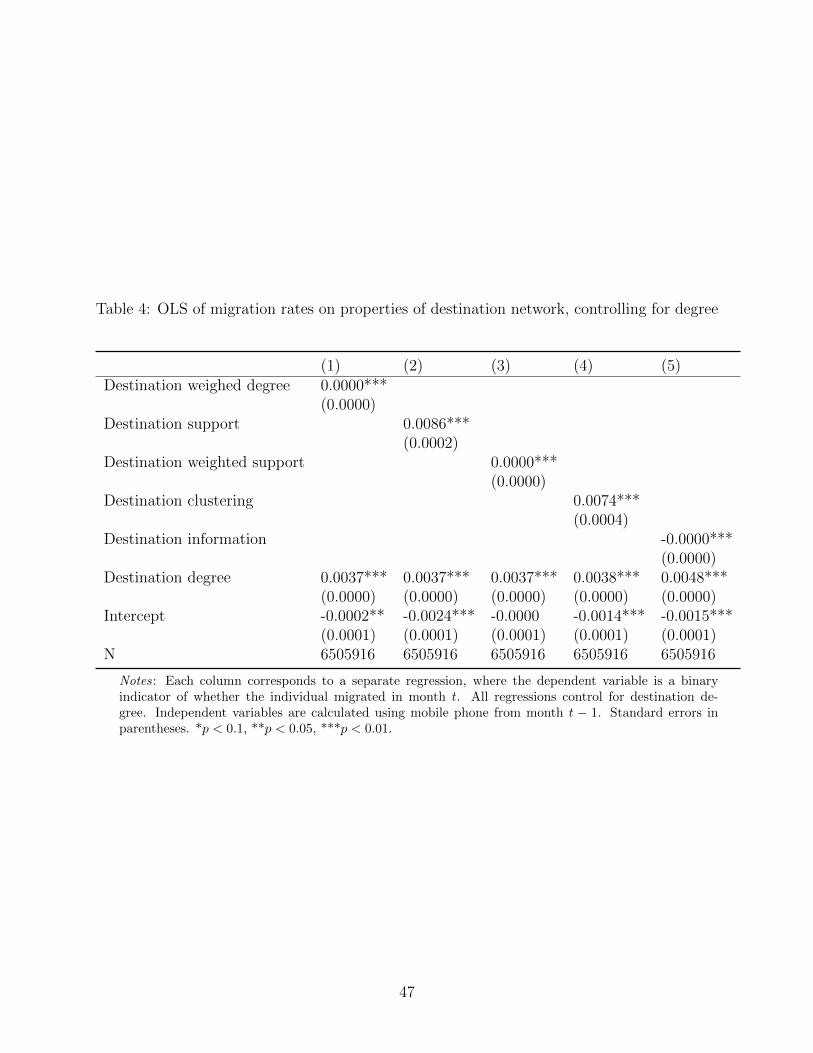
Table 4: OLS of migration rates on properties of destination network, controlling for degree
(1) (2) (3) (4) (5)Destination weighed degree 0.0000***
(0.0000)Destination support 0.0086***
(0.0002)Destination weighted support 0.0000***
(0.0000)Destination clustering 0.0074***
(0.0004)Destination information -0.0000***
(0.0000)Destination degree 0.0037*** 0.0037*** 0.0037*** 0.0038*** 0.0048***
(0.0000) (0.0000) (0.0000) (0.0000) (0.0000)Intercept -0.0002** -0.0024*** -0.0000 -0.0014*** -0.0015***
(0.0001) (0.0001) (0.0001) (0.0001) (0.0001)N 6505916 6505916 6505916 6505916 6505916
Notes: Each column corresponds to a separate regression, where the dependent variable is a binaryindicator of whether the individual migrated in month t. All regressions control for destination de-gree. Independent variables are calculated using mobile phone from month t − 1. Standard errors inparentheses. *p < 0.1, **p < 0.05, ***p < 0.01.
47
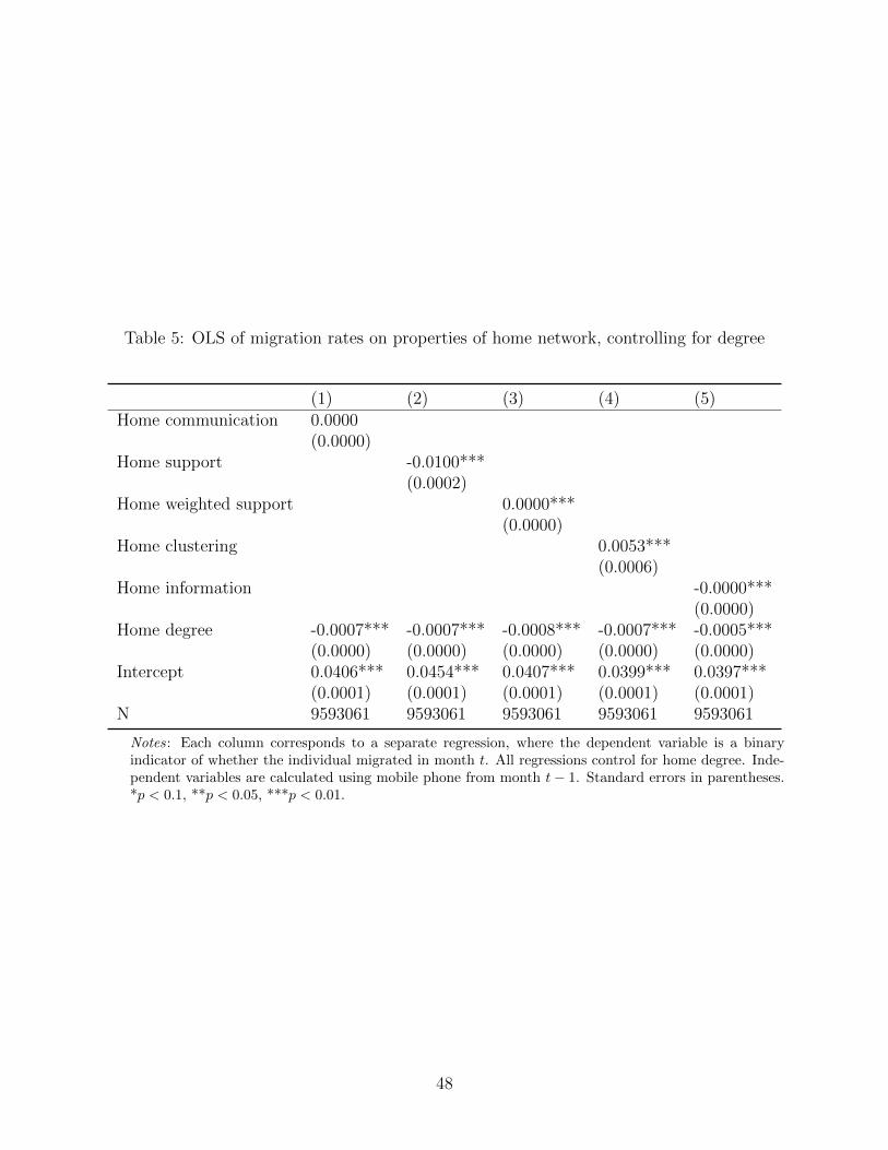
Table 5: OLS of migration rates on properties of home network, controlling for degree
(1) (2) (3) (4) (5)Home communication 0.0000
(0.0000)Home support -0.0100***
(0.0002)Home weighted support 0.0000***
(0.0000)Home clustering 0.0053***
(0.0006)Home information -0.0000***
(0.0000)Home degree -0.0007*** -0.0007*** -0.0008*** -0.0007*** -0.0005***
(0.0000) (0.0000) (0.0000) (0.0000) (0.0000)Intercept 0.0406*** 0.0454*** 0.0407*** 0.0399*** 0.0397***
(0.0001) (0.0001) (0.0001) (0.0001) (0.0001)N 9593061 9593061 9593061 9593061 9593061
Notes: Each column corresponds to a separate regression, where the dependent variable is a binaryindicator of whether the individual migrated in month t. All regressions control for home degree. Inde-pendent variables are calculated using mobile phone from month t− 1. Standard errors in parentheses.*p < 0.1, **p < 0.05, ***p < 0.01.
48
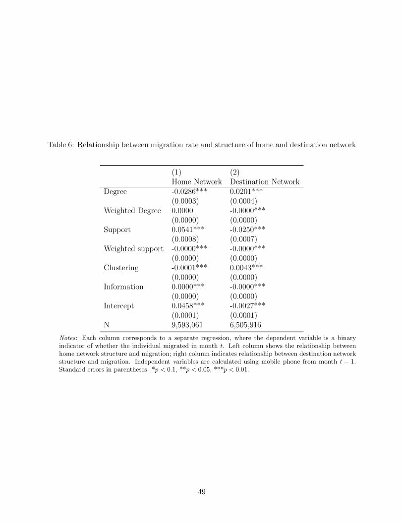
Table 6: Relationship between migration rate and structure of home and destination network
(1) (2)Home Network Destination Network
Degree -0.0286*** 0.0201***(0.0003) (0.0004)
Weighted Degree 0.0000 -0.0000***(0.0000) (0.0000)
Support 0.0541*** -0.0250***(0.0008) (0.0007)
Weighted support -0.0000*** -0.0000***(0.0000) (0.0000)
Clustering -0.0001*** 0.0043***(0.0000) (0.0000)
Information 0.0000*** -0.0000***(0.0000) (0.0000)
Intercept 0.0458*** -0.0027***(0.0001) (0.0001)
N 9,593,061 6,505,916
Notes: Each column corresponds to a separate regression, where the dependent variable is a binaryindicator of whether the individual migrated in month t. Left column shows the relationship betweenhome network structure and migration; right column indicates relationship between destination networkstructure and migration. Independent variables are calculated using mobile phone from month t − 1.Standard errors in parentheses. *p < 0.1, **p < 0.05, ***p < 0.01.
49
Data: Call detail records with mobile base towersResult: Monthly modal district
Step 1 Find each subscriber’s most frequently visited tower calculate overall dailymodal districts ;
calculate overall monthly modal districts ;
Step 2 calculate the hourly modal districts ;if tie districts exit then
if overall daily modal districts can resolve thenreturn the district with larger occurance number;else
if overall monthly modal districts can resolve thenreturn the district with larger occurance number
end
end
end
end
Step 3 calculate the daily modal districts ;if tie districts exit then
if overall daily modal districts can resolve thenreturn the district with larger occurance number;else
if overall monthly modal districts can resolve thenreturn the district with larger occurance number
end
end
end
end
Step 4 calculate the monthly modal districts ;if tie districts exit then
if overall monthly modal districts can resolve thenreturn the district with larger occurance number;
end
endAlgorithm 1: Home location assignment
50
Data: Monthly modal district for four consecutive months: D1, D2, D3, D4
Result: Migration type
if D1 == D2 AND D3 == D4 thenif D2 == D3 then
if D4 == Kigali thenmigration type is urban resident
endelse
migration type is rural residentend
endelse
if D4 == Kigali thenmigration type is rural to urban
endelse
if D1 == Kigali thenmigration type is urban to rural
endelse
migration type is rural to ruralend
end
end
endelse
migration type is otherend
Algorithm 2: Classifying individuals by migrant type for k=2
51
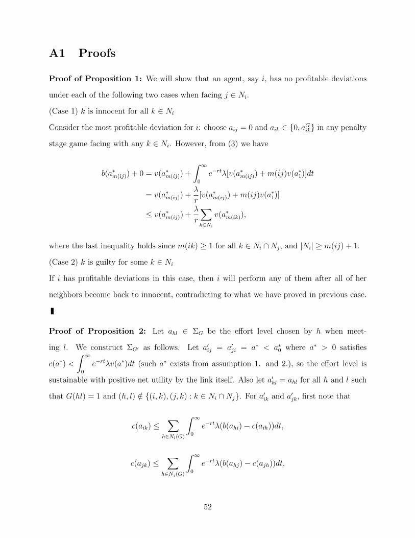
A1 Proofs
Proof of Proposition 1: We will show that an agent, say i, has no profitable deviations
under each of the following two cases when facing j ∈ Ni.
(Case 1) k is innocent for all k ∈ Ni
Consider the most profitable deviation for i: choose aij = 0 and aik ∈ {0, aGik} in any penalty
stage game facing with any k ∈ Ni. However, from (3) we have
b(a∗m(ij)) + 0 = v(a∗m(ij)) +
∫ ∞0
e−rtλ[v(a∗m(ij)) +m(ij)v(a∗1)]dt
= v(a∗m(ij)) +λ
r[v(a∗m(ij)) +m(ij)v(a∗1)]
≤ v(a∗m(ij)) +λ
r
∑k∈Ni
v(a∗m(ik)),
where the last inequality holds since m(ik) ≥ 1 for all k ∈ Ni ∩Nj, and |Ni| ≥ m(ij) + 1.
(Case 2) k is guilty for some k ∈ Ni
If i has profitable deviations in this case, then i will perform any of them after all of her
neighbors become back to innocent, contradicting to what we have proved in previous case.
Proof of Proposition 2: Let ahl ∈ ΣG be the effort level chosen by h when meet-
ing l. We construct ΣG′ as follows. Let a′ij = a′ji = a∗ < a∗0 where a∗ > 0 satisfies
c(a∗) <
∫ ∞0
e−rtλv(a∗)dt (such a∗ exists from assumption 1. and 2.), so the effort level is
sustainable with positive net utility by the link itself. Also let a′hl = ahl for all h and l such
that G(hl) = 1 and (h, l) /∈ {(i, k), (j, k) : k ∈ Ni ∩Nj}. For a′ik and a′jk, first note that
c(aik) ≤∑
h∈Ni(G)
∫ ∞0
e−rtλ(b(ahi)− c(aih))dt,
c(ajk) ≤∑
h∈Nj(G)
∫ ∞0
e−rtλ(b(ahj)− c(ajh))dt,
52
c(akl) ≤∑
h∈Nk(G)
∫ ∞0
e−rtλ(b(ahk)− c(akh))dt for l ∈ {i, j}.
Consider ε > 0 such that Cl <
∫ ∞0
e−rtλ
(v(a∗) +
∑h∈Ni∩Nj
(c(alh)− c(alh + ε)
))dt where
Cl ∈ {c(a∗), c(alk + ε) − c(alk)} and l ∈ {i, j}. Choosing a′ik = aik + ε, a′jk = ajk + ε,
a′ki = aki, and a′kj = aki satisfies the incentive constraints among i, j, and those k’s with
clk(G′) > clk(G):
c(a′ik) < c(aik) +
∫ ∞0
e−rtλ
(v(a∗) +
∑h∈Ni∩Nj
(c(aih)− c(a′ih)
))dt
≤∫ ∞0
e−rtλ( ∑h∈Ni(G)
(b(ahi)− c(aih)
)+ v(a∗) +
∑h∈Ni∩Nj
(c(aih)− c(a′ih)
))dt
=∑
h∈Ni(G′)
∫ ∞0
e−rtλ(b(a′hi)− c(a′ih))dt,
c(a′jk) ≤∑
h∈Nj(G′)
∫ ∞0
e−rtλ(b(a′hj)− c(a′jh))dt,
c(a′ij) = c(a′ji) = c(a∗) <
∫ ∞0
e−rtλ
(v(a∗) +
∑k∈Ni∩Nj
(c(aik)− c(a′ik)
))dt
≤∫ ∞0
e−rtλ
(v(a∗) +
∑k∈Ni∩Nj
(c(aik)− c(a′ik)
)+
∑h∈Ni(G)
(b(ahi)− c(aih)))dt
=
∫ ∞0
e−rtλv(a∗)dt+∑
h∈Ni(G)
∫ ∞0
e−rtλ(b(a′hi)− c(a′ih))dt,
c(a′kl) = c(akl) ≤∑
h∈Nk(G)
∫ ∞0
e−rtλ(b(ahk)− c(akh))dt
<∑
h∈Nk(G′)
∫ ∞0
e−rtλ(b(a′hk)− c(a′kh))dt,
where l ∈ {i, j} and a′ik > aik and a′jk > ajk yields the last (strict) inequality. For all other
remaining incentive constraints, they are satisfied since their counterparts in ΣG hold by
definition. To complete the construction of ΣG′ , if someone deviated, then all her neighbors
use the social norm with sequential move described before Proposition 1 to punish the
53
deviator.
By the construction of this new equilibrium ΣG′ , we have
uk(ΣG′) =∑
h∈Nk(G′)
∫ ∞0
e−rtλ(b(a′hk)− c(a′kh)))dt
>∑
h∈Nk(G)
∫ ∞0
e−rtλ(b(ahk)− c(akh)))dt = uk(ΣG).
for all k ∈ Ni ∩Nj.
Proof of Proposition 3: For notational convenience, we define ∆ = λ′ij−λij, Nij = Ni∩Nj,
vi = b(aji) − c(aij), and vj = b(aij) − c(aji). Let k ∈ Nij and ahl ∈ Σλ be the effort level
chosen by h when meeting l. We construct Σλ′ as follows. Without loss of generality, assume
vi > 0. (If vi = 0, we can sustain an equilibrium by increasing both aij and aji to make the
assumption hold without decreasing any agent’s utility). Also let a′hl = ahl for all h and l
such that G(hl) = 1 and (h, l) /∈ {(i, k), (j, k) : k ∈ Ni ∩Nj}. For a′ik and a′jk, first note that
c(aik) ≤∑
h∈Ni(G)
∫ ∞0
e−rtλih(b(ahi)− c(aih))dt,
c(ajk) ≤∑
h∈Nj(G)
∫ ∞0
e−rtλjh(b(ahj)− c(ajh))dt,
c(akl) ≤∑
h∈Nk(G)
∫ ∞0
e−rtλkh(b(ahk)− c(akh))dt for l ∈ {i, j}.
If vj ≤ 0, then choose η ≥ 0 such that a′ij , aij + η = aji with v′i = b(aji)− c(a′ij) > 0 (Such
η exists since vi + vj > 0); if not, then let η = 0. Given η, there exists ε > 0 such that
∫ ∞0
e−rt(
∆v′i +∑h∈Nij
λih(c(aih)− c(aih + ε)
)+ λij(c(aij)− c(a′ij))
)dt ≥ c(aij + η)− c(aij),
∫ ∞0
e−rt(
∆v′i +∑h∈Nij
λih(c(aih)− c(aih + ε)
)+ λij(c(aij)− c(a′ij))
)dt ≥ c(aik + ε)− c(aik),
54
for all k ∈ Nij. Define a′ik = aik + ε, a′jk = ajk, a′ki = aki, a
′kj = akj, and a′ji = aji, then the
incentive constraints among i, j, and those k’s in Nij are satisfied:
c(a′ik) ≤ c(aik) +
∫ ∞0
e−rt(
∆v′i +∑h∈Nij
λih(c(aih)− c(a′ih)
)+ λij(c(aij)− c(a′ij))
)dt
≤∫ ∞0
e−rt(∑h∈Ni
λih(b(ahi)− c(aih)
)+ ∆v′i +
∑h∈Nij∪{j}
λih(c(aih)− c(a′ih)
))dt
=∑h∈Ni
∫ ∞0
e−rtλ′ih(b(a′hi)− c(a′ih))dt,
c(a′ij) ≤∑h∈Ni
∫ ∞0
e−rtλ′ih(b(a′hi)− c(a′ih))dt,
c(a′jk) = c(ajk) ≤∑h∈Nj
∫ ∞0
e−rtλjh(b(ahj)− c(ajh))dt ≤∑h∈Nj
∫ ∞0
e−rtλ′jh(b(a′hj)− c(a′jh))dt,
c(a′ji) = c(aji) ≤∑h∈Nj
∫ ∞0
e−rtλ′jh(b(a′hj)− c(a′jh))dt,
c(a′kl) = c(akl) ≤∑h∈Nk
∫ ∞0
e−rtλkh(b(ahk)− c(akh))dt
≤∑h∈Nk
∫ ∞0
e−rtλkh(b(a′hk)− c(a′kh))dt
=∑h∈Nk
∫ ∞0
e−rtλ′kh(b(a′hk)− c(a′kh))dt,
where l ∈ {i, j}. For all other remaining incentive constraints, they are satisfied since their
counterparts in Σλ hold by definition. From this new equilibrium Σλ′ , we have
uk(Σλ′) =∑h∈Nk
∫ ∞0
e−rtλ′kh(b(a′hk)− c(a′kh))dt
>∑h∈Nk
∫ ∞0
e−rtλkh(b(ahk)− c(akh))dt = uk(Σλ).
55
for all k ∈ Nij ∪ {j}; particularly for i, we have
ui(Σλ′) =∑h∈Ni
∫ ∞0
e−rtλ′ih(b(a′hi)− c(a′ih))dt
=
∫ ∞0
e−rt∆v′idt+∑h∈Ni
∫ ∞0
e−rtλih(b(a′hi)− c(a′ih))dt
=
∫ ∞0
e−rt∆v′idt+∑
h∈Nij∪{j}
∫ ∞0
e−rtλih(c(aih)− c(a′ih))dt+ ui(Σλ)
> ui(Σλ).
56