November 11, 2011 - PacDev 2018 at UC Davis - About the ... Is couple’s joint decision making associated with favorable household consumption patterns for children? Evidence from

1

Is couple’s joint decision making associated with favorable

household consumption patterns for children? Evidence from Cebu, Philippines

J.M. Ian Salas∗

November 11, 2011

Abstract

Using a cross-sectional dataset from a set of communities in Cebu province, Philippines, this

paper seeks to characterize the relationship between a couple’s decision-making arrangement

and their household’s consumption pattern. I construct indices of the mother’s and the father’s

prevalence in decision making based on the proportion of important decision-making situations

wherein the mother and the father each became solely decisive, while allowing for a distinct third

category of joint decision making, a proxy for cooperative spousal behavior. After controlling

for total household resources and several factors that influence each spouse’s bargaining power, the estimates I obtain from a system of demand functions for household consumption goods

suggest that, relative to sole decision making by either parent, joint decision making is related

to favorable spending patterns for children (higher budget shares on milk, schooling, medicine, and clothing and lower budget shares on beverages and alcohol). In addition, the mother and the

father do not seem to exhibit conflicting preferences across a range of household consumption

goods, so that it is likely that joint decision making allows couples to coordinate their resource

allocation decisions and mitigate the underprovision of household public goods. JEL classification: D13, D12, D70, J12, J13

Keywords: joint decision making, cooperative spousal behavior, intrahousehold resource allocation, household bargaining models

Introduction

Interest in the analysis of decision making within the household has mainly focused on tracing

out how the balance of bargaining power between spouses affects household resource allocation

decisions. Many empirical studies have established that mother-specific income changes tend to

increase spending on children’s goods and human development, while father-specific income changes

∗Ph.D. student, Department of Economics, University of California, Irvine. Email: [email protected]. Many thanks to Daisy Carreon, Amihai Glazer, Monica Mananzan, David Neumark, and Priya Ranjan for helpful comments. Financial support from the UCI Department of Economics and the UCLA Institute for Research on Labor and Employment are gratefully acknowledged.

1

mailto:[email protected]

tend to increase spending on vices, e.g. alcohol and tobacco (Haddad, Hoddinott and Alderman

[14]; Bobonis [2] for recent evidence in a randomized experiment setting). In addition, relatively

higher income or assets in the hands of mothers is associated with improved outcome measures such

as better household nutrition and health, and enhanced anthropometric development and survival for children (Thomas [20]). These findings support the belief that mothers care for their children’s

well-being more than fathers do,1 and underpin policies that encourage improvements in women’s

bargaining power relative to their partner or spouse.2

The key assumption in cooperative bargaining models that attempt to provide a theoretical basis for this literature is that mothers and fathers have distinct preferences, and that their relative

bargaining strength determines the extent by which each spouse’s preferred resource allocation gets

implemented in the final outcome. In this setup, if agreement is reached, an application of the Nash

bargaining solution concept is used to propose a possible efficient equilibrium outcome; if agreement

is not reached, bargaining breaks down and the couple settles for an inefficient noncooperative

outcome with voluntary contributions to the household public good.3

Note that in much of the empirical analysis of household decision making, the role of spousal agreement in attaining an efficient outcome has been largely unexplored, if not ignored. Most

research has been involved in reduced-form investigations of how bargaining strength, a necessarily adversarial or zero-sum construct, relates to the eventual outcome, regardless of whether the

outcome is efficient or not.4

In this paper, I attempt to fill this gap by considering decision-making arrangements that

characterize a couple’s propensity to agree and make household decisions together (joint decision

making) or apart (sole decision making by the mother or father). This decision-making arrangement

is a description of the outcome of the decision-making process and can be interpreted as a measure of the extent of cooperative behavior or engagement among spouses. The paper’s goal is to determine

if this measure of spousal cooperation can be demonstrably linked to distinct spending patterns

that characterize benign outcomes for children. Figure 1 illustrates how this paper’s approach

differs from the present literature. Using a cross-sectional dataset from a set of communities in Cebu province, Philippines, I find

that compared to households where sole decision making by either parent is prevalent, the consumption patterns in households where joint spousal decision making is practiced more intensively

1Several papers, however, have noted that these findings may apply only up to a point; they provide evidence that when women have much greater bargaining power than men, results get reversed such that spending on children and school enrollment are lower (Felkey [9], Gitter and Barham [12], and Lancaster, Maitra, and Ray [16]). This implies that household welfare is best served when bargaining power is more evenly spread between spouses, although this is not yet relevant in most developing countries where conditions are heavily stacked against women.

2These findings have been influential in the design of aid and welfare programs in poor communities, primarily through micro-credit and cash transfers given to mothers.

3I am interested in the setting wherein marriage continues even if agreement is not reached, so that threat points internal to the marriage are relevant (Lundberg and Pollak [17]). In the long run, the external threat point under divorce or separation that is available to each spouse gains more salience. In the Philippines, the setting of this study, divorce is prohibited, while legal separation is allowed only under very limited circumstances.

4The exception is the “collective” approach championed by Bourguignon, Browning and Chiappori [3], which explicitly tests for Pareto optimality but dispenses with a bargaining setup.

2

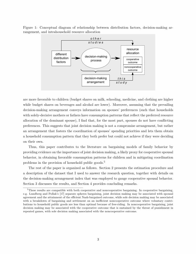
Figure 1: Conceptual diagram of relationship between distribution factors, decision-making arrangement, and intrahousehold resource allocation

o t h e r

s t u d i e s

t h i s

s t u d y

decision-making

process

different

distribution

factors

resource

allocation

cooperative

outcome

noncooperative

outcome

decision-making

arrangement

are more favorable to children (budget shares on milk, schooling, medicine, and clothing are higher

while budget shares on beverages and alcohol are lower). Moreover, assuming that the prevailing

decision-making arrangement conveys information on spouses’ preferences (such that households

with solely-decisive mothers or fathers have consumption patterns that reflect the preferred resource

allocation of the dominant spouse), I find that, for the most part, spouses do not have conflicting

preferences. This suggests that joint decision making is not a compromise arrangement, but rather

an arrangement that fosters the coordination of spouses’ spending priorities and lets them obtain

a household consumption pattern that they both prefer but could not achieve if they were deciding

on their own. Thus, this paper contributes to the literature on bargaining models of family behavior by

providing evidence on the importance of joint decision making, a likely proxy for cooperative spousal behavior, in obtaining favorable consumption patterns for children and in mitigating coordination

problems in the provision of household public goods.5

The rest of the paper is organized as follows. Section 2 presents the estimation procedure and

a description of the dataset that I used to answer the research question, together with details on

the decision-making arrangement index that was employed to gauge cooperative spousal behavior. Section 3 discusses the results, and Section 4 provides concluding remarks.

5These results are compatible with both cooperative and noncooperative bargaining. In cooperative bargaining, e.g. Lundberg and Pollak’s [17] separate spheres bargaining, joint decision making may be associated with spousal agreement and the attainment of the efficient Nash-bargained outcome, while sole decision making may be associated with a breakdown of bargaining and settlement on an inefficient noncooperative outcome where voluntary contributions to household public goods are less than optimal because of free-riding. In noncooperative bargaining, joint decision making may be associated with the cooperative outcome that is sustained by the threat of punishment in repeated games, with sole decision making associated with the noncooperative outcome.

3

2 Data and estimation

This section covers the econometric methodology used in this paper to estimate household demand

functions for consumption goods, and then provides details on the variables used from the cross-sectional dataset that was employed to look at the prevalence of joint spousal decision making and

how it correlates with household consumption patterns.

2.1 Estimation procedure

I model households’ demand for different consumption goods as a function of the couple’s decision-making arrangement, total household resources, individual and household characteristics, wages, and prices. I estimate the following system of demand functions:

ln(qji) = αj + βj1z1i + βj2z2i + ln(xi) + ciγj + Eji, (1)

where qji is the expenditure share on consumption good j for household i, z1i and z2i are the

two indices of the decision-making arrangement,6 xi is the level of aggregate household resources, the vector ci denote a set of household and individual member controls, and Eji are unobservable

determinants of household demand for each good j. Total household consumption expenditure is

used for xi, which is instrumented by measures of household income to address potential endogeneity

concerns. Because wages and prices are available only at the village level, I first estimate models

where they are part of the residual, and include them later as part of a robustness exercise. To allow for correlation of disturbances among the different goods, the seemingly unrelated

regression (SUR) model is used to estimate system of functions (1), with standard errors that are

adjusted for clustering at the village level. While the log-transformation used for the expenditure share above does not correspond to a

proper demand system as in the Almost Ideal Demand System (AIDS) by Deaton and Muellbauer

[8], I adopt it for its capability to handle outliers and heteroskedasticity and also for convenience

in the interpretation of the model coefficient estimates.7

2.2 Cebu Longitudinal Health and Nutrition Survey

The data I use is from the 1994-1995 follow-up round of the Cebu Longitudinal Health and Nutrition

Survey (CLHNS).8 The CLHNS tracks an original sample of 3,327 Filipino women who gave birth

6Since I classify each decision situation as being decided by the mother, the father, or both spouses, I adopt a three-way classification for the couple’s decision-making arrangement, which then requires two indices in order to be identified; further details are provided in the next subsection.

7This comes at a price of being unable to impose an adding up restriction, such that the implied predicted expenditure shares on the different consumption goods do not necessarily sum up to unity. Bobonis [2] used a similar functional form for the budget share, although he adopted more flexible functional forms (i.e. polynomials) for total household resources.

8It is part of an ongoing study conducted by the Carolina Population Center of the University of North Carolina at Chapel Hill, in collaboration with the Office of Population Studies of the University of San Carlos and the Nutrition Center of the Philippines. The data files and codebooks are publicly available and can be accessed from

4

between May 1, 1983 and April 30, 1984 in 33 randomly selected barangays (villages) in and around

Cebu City, the second largest city in the Philippines and the capital of the island province with the

same name. The CLHNS initially looked into infant feeding determinants and practices (1984-1986), but was

later on extended to include detailed questions on, among others things, intellectual and nutritional development of the children (1991-1992); women’s status, family planning use and labor force

participation (1994-1995); adolescent reproductive health and sexual behavior (1998-1999); and

educational attainment, work patterns, and wages of young adults (2002 and 2005). Modules on household expenditures and household decision-making were both included in the

1994-1995 round,9 when the index children (those born during the sample window) have turned

11 years old. I used these modules to construct the components of the demand system and the

decision-making arrangement, while other modules provided the data for household and individual control variables.

The sample households in the CLHNS live in a culturally homogeneous location, with 1990

census figures both placing Cebuano ethnicity and Roman Catholic religious affiliation at more

than 95 percent of the population in Cebu City and the larger Cebu province.10 Thus, it is likely

that the sample households share the same values and norms and that concerns about comparability

across communities, as expressed by Ghuman, Lee and Smith [13], will be at a minimum.

2.2.1 Decision-making arrangement indices

The household decision-making module in the CLHNS contained questions that asked the mother

how decisions were made regarding different household situations, including identifying who was

involved in decision making and whose will prevailed in each particular situation. The questionnaire

did not restrict respondents to name just one person as the ultimate decision maker, and also

allowed respondents to name household and family members other than the mother and the father

in the decisive set. In the majority of cases, the respondents indicated that the final decision was

made by one of the following: just the mother, just the father, or both spouses deciding jointly.11

These three responses enable me to ascertain the decision-making arrangement prevailing in the

household, where joint spousal decision making constitutes an arrangement that is separate and

distinct from mother or father decisiveness. I selected five situations which (i) plausibly solicit discussion and negotiation between spouses,12

and which were (ii) least likely to be subject to disinterested decision making by either spouse: buy

<www.cpc.unc.edu/projects/cebu>.9While the Philippines’ Demographic and Health Survey (DHS) also contains information on household decision

making, it is not suitable for this paper’s research question because it lacks household expenditure data.10The survey sample reflects this religious homogeneity (ethnicity was not asked in the survey). 11As will be explained in the next subsection, I will restrict my attention to households that only had these

responses.12Lack of involvement is likely to arise in situations where gender-specific roles are strong (e.g., Cabaraban and

Morales [5] find that traditional norms give Filipino women control over subsistence resource allocation decisions, while Filipino men exert control over decisions involving large/expensive items such as durables). Lundberg and Pollak [17] point out that a division of responsibilities based on gender roles likely emerges without explicit bargaining.

5

http://www.cpc.unc.edu/projects/cebu

Table 1: Indicators of marital quality as a function of decision-making arrangement Independent variables Dependent variable

Father physically Decision-making hurts mother when Father takes care arrangement index: he gets angry of the children

Joint relative to mother −.224*** −.193*** −.002 .028 (.039) (.054) (.030) (.034)

Joint relative to father −.123** −.094+ .083** .113*** (.054) (.065) (.034) (.042)

Constant .022 .038+ .127*** .143*** (.019) (.026) (.017) (.015)

Village-level fixed effects No Yes No Yes N = 1, 322 households

Note: The table presents coefficient estimates and standard errors from a linear probability model, with disturbance terms clustered at the village level. The sample is composed of nuclear households which had the mother or father (or both) prevail in deciding each of the following five situations: buying or selling land, practicing family planning, mother working outside the home, mother traveling outside the province, and spending of mother’s earnings. Significance indicated at the following confidence levels: + 85 percent; * 90 percent; ** 95 percent; *** 99 percent.

ing or selling land, practicing family planning, mother working outside the home, mother traveling

outside the province, and spending of mother’s earnings. I then constructed two indices that capture the proportion of situations wherein the mother and the father each became solely decisive,13

with joint decision making as an omitted category. I use these indices as proxies for the decision-making arrangement, which can be thought of as

a description of the outcome of the decision-making process14 in terms of the extent of cooperative

behavior or engagement among spouses. In addition, these indices may also capture certain aspects

of marital quality. Using the full sample of nuclear households with eligible responses, Table 1

shows that in households where joint decision making is practiced more intensively relative to

father sole decisiveness, the chances of wife physical abuse are slimmer, while the likelihood of father involvement in child care is higher.15

It is noteworthy that previous attempts to describe the decision-making process within the

household portray spouses as largely having adversarial relations, such that an increase in one

person’s bargaining power allows him/her to exert more influence in decision making and extract

13Note that it was possible to relax this and look into the proportion of situations wherein either the mother and/or the father was involved in decision making, regardless of who prevailed at the end. This approach couldn’t be used reliably since the questionnaire was structured in such a way that the interviewer inquired first who were consulted by the mother in decision making before asking whose will prevailed; this resulted in the mother being automatically involved in decision making in each situation.

14In this sense, I utilize information that is closer to the decision-making process than other variables that try to measure bargaining power.

15Note that the finding on reduced likelihood of wife physical abuse also applies when comparing joint decision making to mother sole decisiveness. While some might find this surprising, it becomes plausible if one entertains the possibility that some fathers become abusive not only when they feel dominant but also when they feel dominated. This finding supports the contention that a three-way classification is better because it uncovers subtleties not seen in a typical two-way analysis.

6

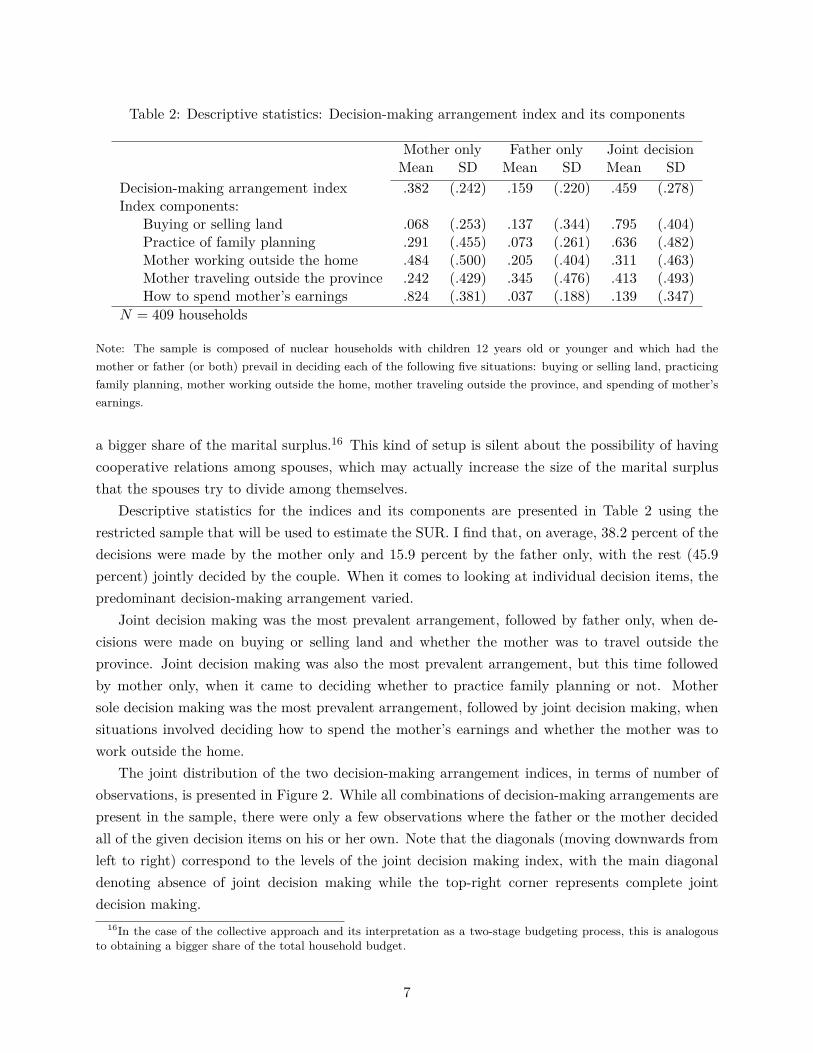
Table 2: Descriptive statistics: Decision-making arrangement index and its components

Mother only Father only Joint decision Mean SD Mean SD Mean SD

Decision-making arrangement index .382 (.242) .159 (.220) .459 (.278) Index components:

Buying or selling land .068 (.253) .137 (.344) .795 (.404) Practice of family planning .291 (.455) .073 (.261) .636 (.482) Mother working outside the home .484 (.500) .205 (.404) .311 (.463) Mother traveling outside the province .242 (.429) .345 (.476) .413 (.493) How to spend mother’s earnings .824 (.381) .037 (.188) .139 (.347)

N = 409 households

Note: The sample is composed of nuclear households with children 12 years old or younger and which had the

mother or father (or both) prevail in deciding each of the following five situations: buying or selling land, practicing

family planning, mother working outside the home, mother traveling outside the province, and spending of mother’s

earnings.

a bigger share of the marital surplus.16 This kind of setup is silent about the possibility of having

cooperative relations among spouses, which may actually increase the size of the marital surplus

that the spouses try to divide among themselves. Descriptive statistics for the indices and its components are presented in Table 2 using the

restricted sample that will be used to estimate the SUR. I find that, on average, 38.2 percent of the

decisions were made by the mother only and 15.9 percent by the father only, with the rest (45.9

percent) jointly decided by the couple. When it comes to looking at individual decision items, the

predominant decision-making arrangement varied. Joint decision making was the most prevalent arrangement, followed by father only, when de

cisions were made on buying or selling land and whether the mother was to travel outside the

province. Joint decision making was also the most prevalent arrangement, but this time followed

by mother only, when it came to deciding whether to practice family planning or not. Mother

sole decision making was the most prevalent arrangement, followed by joint decision making, when

situations involved deciding how to spend the mother’s earnings and whether the mother was to

work outside the home. The joint distribution of the two decision-making arrangement indices, in terms of number of

observations, is presented in Figure 2. While all combinations of decision-making arrangements are

present in the sample, there were only a few observations where the father or the mother decided

all of the given decision items on his or her own. Note that the diagonals (moving downwards from

left to right) correspond to the levels of the joint decision making index, with the main diagonal denoting absence of joint decision making while the top-right corner represents complete joint

decision making. 16In the case of the collective approach and its interpretation as a two-stage budgeting process, this is analogous

to obtaining a bigger share of the total household budget.

7

Figure 2: Joint distribution of decision-making arrangement indices, Number of observations

2247452

672216126

5540209

43189

319

8

0

.2

.4

.6

.8

1

Mot

her

sole

−de

cisi

vene

ss in

dex

0.2.4.6.81Father sole−decisiveness index

N = 409 households

Note that while the two indices capture the extent by which the three different decision-making

arrangements are prevalent in each household, the discussion in the next section will focus on

comparing the extremes, i.e. sole decision making by either parent versus joint decision making, for ease of interpretation.17

Because mothers were the only respondents in the survey, I rely exclusively on mother-reported

evaluations for the construction of the decision-making arrangement indices.18 Ghuman, Lee and

Smith [13] warn about the validity of similar approaches in the context of measuring women’s

autonomy, mainly because spouses’ responses were not always consistent when they were independently asked the same questions pertinent to gauging the woman’s level of autonomy. They

conclude that it is likely that the questions do not have the same cognitive or semantic meaning

to men and women, which brings up the question of what, if anything, it is measuring.19 However, unlike other research that ascribes values of women’s autonomy and empowerment to responses

to these decision-making questions, I utilize mother’s responses here as simply a gauge, however

imprecise, of whether cooperative behavior is present in the household or not, and it is sufficient

for my purposes that one spouse thinks this is so.20 At any rate, if measurement error is present in

mother’s reporting, then it is expected that attenuation bias will make it harder to get statistically

significant estimates. 17Keep in mind that the regression estimates come from considering all of the different combinations present in the

sample.18The only item in the survey that asks about differential couple preferences is each spouse’s preference for having

more children, of which there was 82 percent agreement.19This does not mean, however, that mother-reported evalutions are useless; in fact, the authors mention that in

some cases, such as in relating women’s autonomy to child mortality, mother’s self-reports “appear to have some criterion-based validity.”

20Thus, reports of joint decision making need not be consistent for both spouses.

8

2.2.2 Sample restrictions

While the CLHNS started out with 3,327 mother and child pairs in the original sample, only 2,483

households were re-interviewed in the 1994-1995 round,21 mainly because of attrition due to outmigration.22 From this number, I imposed particular sample restrictions that allow me to address

my research question with the least amount of ambiguity. As a practical matter, I used the sample of households which had the parents of the index child

(those born during the initial sample window) both alive and living together. I then restricted the

sample to households which had nuclear family living arrangements, so that the estimated demand

functions for consumption goods can be attributed to consumption only by the couple and their

children. To ensure that no outside person is influential in the decision-making process, I restricted

the sample further to households which had either the mother or the father (or both) prevail in

deciding each of the five situations mentioned above.23 This allows me to interpret the negative

of the coefficient estimates as the full impact of shifting away from either mother or father sole

decisiveness towards joint decision making. Lastly, I only consider households with children who are 12 years old (when children are typically

at the last year of elementary school) or younger. This restriction affords me several advantages: children are less likely to directly influence decision making the younger they are; some household

expenditure categories can be successfully assigned to the parents; and it further homogenizes my

sample in that all the households I consider are similarly situated in terms of rearing young children. After imposing all these sample restrictions, I ended up with a sample of 409 households.

2.2.3 Household resources and demand system components

Various items from the household income and expenditures modules were consolidated and converted to common (monthly) units to come up with the values for total household resources and

consumption expenditure that will be used in estimating the system of demand functions. Table

3 presents the average household income, in-kind transfers, and expenditures and the expenditure

shares of the different household consumption goods. Total household income was computed as the sum of the following income categories: wage

income, self-employment income, net income from agricultural activities24 (composed of farming, fishing, livestock raising, and home gardening), and income from other sources (property rental, pension and dividends, and cash remittances from relatives). Because it is possible that in-kind

transfers of food and clothing received by the household may also affect its level of consumption

expenditures, especially for poorer households, I include it, together with total household income, 21The survey tried to follow the mother and the index child in their new households if they were separated for any

reason. 22Feranil, Gultiano and Adair [10] mention that attrition has resulted in a bias “towards rural and poor households

with fewer modern amenities or assets and less educated parents.” 23Indeed, for some households and in some situations, parents-in-law or other relatives acted as decision makers. 24This includes the value of own consumption.

9

as instruments in the first stage regression of total consumption expenditure.25

Average monthly total household income for the sample was rather limited at 5,787 pesos ($230

using the exchange rate prevailing at that time), while average monthly total household expenditure

was 5,184 pesos ($205), with 3,952 pesos ($155) going to consumption. The average value of monthly

in-kind transfers received was rather low at 161 pesos ($7). The 16 consumption expenditure categories are also listed in Table 3, arranged according to

groupings by food (cereal and grains, meat and seafood, milk and milk products, vegetable and

fruits, ready-cooked food, other food, and beverages), goods typically preferred by fathers (alcohol, tobacco, and transportation), goods typically preferred by mothers (hygiene, clothing, and

medicine), and other public goods from the parents’ point of view (child allowance, schooling, and

recreation).26 Details on the example items under each category are available in Appendix C. While all the data on the expenditure items in the CLHNS were collected only at the household

level, I can safely assign four consumption categories to particular household members: child allowance and schooling for children, and alcohol and tobacco for the parents. All the rest are treated

as collective goods. On average, food items account for about 69.5 percent of monthly total household consumption

expenditures. This is dominated by cereal and grains (23.1 percent) and meat and seafood (22.1

percent), with the rest going to ready-cooked food (6.1 percent), other food (5.5 percent), vegetable

and fruits (5.1 percent), beverages (4.6 percent), and milk and milk products (3.0 percent). The remaining 30.5 percent of total household consumption expenditures are allotted, on aver

age, in the following manner: 5.6 percent go to hygiene, 5.3 percent go to transportation, 4.1 go to

child allowance, 3.4 percent go to schooling, 3.1 percent go to tobacco, 2.7 percent go to clothing, 2.4 percent go to alcohol, 2.1 percent go to medical expenditures, and 1.7 percent go to recreation.

2.2.4 Basic set of control variables

Table 4 presents the descriptive statistics for the basic set of controls used in all subsequent regressions. These controls include age, education, and employment characteristics of the mother and

father, the age distribution and school attendance of children, and several household characteristics. Based on the average age at marriage27 of 22 years for females and 25 for males, about half of

the mothers (50.6 percent) and a little more than half of the fathers (56.2 percent) in the sample

had children at an age younger than average at the time when they were first surveyed. In terms of education, only about a quarter of fathers (27.9 percent) and mothers (25.4 percent) in the sample

25All the results that follow are robust to just using total household income as the lone instrument for total consumption expenditure (first-stage F -statistics are highly significant as well).

26I adopt the same order and grouping scheme in the tables that follow. 27Usually, controls for age-related preferences utilize indicator variables for each age group for each spouse. However,

because there was little variation in parent ages (since the sample was based on a cohort of individuals born to families during 1982-1983, there was a concentration of parent ages between 29 and 35 years for mothers and between 30 and 41 years for fathers in the follow-up survey taken in 1994-1995), I decided to use just one indicator variable to control for age-related preferences, with the threshold being the published singulate mean age at marriage (SMAM) for males and females in the country in 1980.

10

Table 3: Descriptive statistics: Household resources and its allocation

Household income Wage income Self-employment income Net income from agricultural activities Income from other sources

Household in-kind transfers received Household expenditure

Consumption expenditure

Food Cereal and grains Meat and seafood Milk and milk products Vegetable and fruits Ready-cooked food Other food Beverages

Goods typically preferred by fathers Alcohol Tobacco Transport

Goods typically preferred by mothers Hygiene Clothing Medicine

Other public goods from parents’ point of view Child allowance Schooling Recreation

Mean SD Total monthly resources (’000 Pesos)

5.787 (4.407) 3.254 (3.534) 1.936 (3.238) .189 (.855) .408 (.882) .161 (.590) 5.184 (3.280) 3.952 (1.888)

Consumption expenditure shares

.231

.221

.030

.051

.061

.055

.046

.024

.031

.053

.056

.027

.021

.041

.034

.017

(.112) (.097) (.042) (.032) (.080) (.024) (.033)

(.036) (.040) (.055)

(.026) (.028) (.040)

(.031) (.035) (.043)

N = 409 households

Note: The sample is composed of nuclear households with children 12 years old or younger and which had the



earnings.

11

Table 4: Descriptive statistics: Control variables Mother’s characteristics Father’s characteristics Mean SD Mean SD

Had children younger than average .506 (.501) .562 (.497) High school graduate or more .254 (.436) .279 (.449) Wage laborer .394 (.489) .714 (.452) Self-employed .374 (.484) .301 (.459) Farm worker .044 (.205) .081 (.273)

No. of boys No. of girls Mean SD Mean SD

Not attending school Age less than 1 year .061 (.240) .064 (.244) Age 1-2 years .183 (.400) .176 (.406) Age 3-4 years .208 (.418) .186 (.396) Age 5-6 years .220 (.449) .200 (.407) Age 7-8 years .071 (.266) .076 (.274) Age 9-10 years .066 (.258) .044 (.269) Age 11-12 years .112 (.324) .078 (.205)

Attending school Age 5-6 years .029 (.169) .042 (.200) Age 7-8 years .225 (.435) .208 (.424) Age 9-10 years .247 (.470) .225 (.435) Age 11-12 years .379 (.543) .359 (.543)

Household characteristics Mean SD

Living in an urban settlement area .709 (.455) Drinking water from piped supply .320 (.467) House connected to electrical system .804 (.397) House has sealed toilet facility .623 (.485) House made of light materials .457 (.499) Living in own house .819 (.385) Living in own lot .161 (.368) Own motor vehicle/s .103 (.304) Own livestock .533 (.500) Own a household business .411 (.493)

Other household variables Mean SD

Marriage length 12.814 (3.543) Mother has remarried .105 (.307) Mother’s children not from the same father .027 (.162) Mother currently breastfeeding .178 (.383) Mother is ill or has been ill in past 3 years .318 (.466) No. of children* with chronic illness/disability .100 (.324) No. of children* hospitalized in past 3 years .088 (.309) N = 409 households

*Information available only for index child and next younger sibling. Note: The sample is composed of nuclear households with children 12 years old or younger and which had the



earnings. 12

3

had completed high school. While 71.4 percent of fathers worked as wage laborers and 30.1 percent were self-employed,

mothers were almost as likely to be self-employed (37.4 percent) as to work for wage labor (39.4

percent). Less than 10 percent of the fathers (8.1 percent) and mothers (4.4 percent) in the sample

were involved in farm work. The average number of children was 3.5, seemingly evenly-distributed by age and gender, al

though there is an expected concentration near 11-12 years because of the sampling basis used in

the survey. Note that there were quite a few children of schooling age who were not attending

school. Seventy-one percent of the sample households were living in an urban settlement area, with 32

percent getting their drinking water from piped supply. Eighty percent of the sample households

had electricity in their homes, 62.3 percent were using sealed toilets, and 45.7 percent were living

in houses constructed from light materials. About 82 percent of the sample households owned the house that they were living in, while 16.1

percent owned the lot where their house was located. About ten percent of the sample households

owned at least one motor vehicle, 53.3 percent owned livestock, and 41.1 percent owned a household

business. Other variables included in the basic set of controls had to do with the couple’s relationship and

indicators that may be relevant to some of the consumption categories. Average marriage length

was 12.8 years, 10.5 percent of mothers have remarried, and 2.7 percent of the sample households

had children who had the same mother but had different fathers.28 Almost 18 percent of mothers

were currently breastfeeding (relevant for spending on milk and milk products), 31.8 percent of mothers were ill or recently ill, an average of 0.1 children were chronically ill or disabled, and an

average of 0.09 children were recently hospitalized (all relevant to medical spending).

Results and discussion

In this section, I present the results from estimating the system of demand functions in (1) using

the CLHNS dataset. I begin by determining the relationship between household consumption

patterns and the decision-making arrangement using a basic set of controls. I then check if the

statistically significant estimates hold up to the inclusion of household-specific distribution factors

and village-level wages and prices in the set of controls. Afterwards, I try to gauge if spouses exhibit

conflicting preferences on different consumption goods, assuming that decisiveness by either parent

in the decision-making arrangement has information content on the decisive parent’s preferences. 28I included this last variable because Browning and Bonke [4] found that having children from before the current

marriage significantly reduces the mother’s share in total resources.

13

3.1 Decision-making arrangement and household consumption patterns

3.1.1 Baseline specification

Table 5 presents estimates from the SUR on the system of demand functions for consumption goods, with controls for log total consumption expenditure and the basic set of controls listed in Table 4. Since joint decision making is omitted in the decision-making arrangement variables, the negative

of the coefficient estimates for mother and father sole decisiveness can be interpreted, conditional on (log) total household consumption expenditure (instrumented by income and in-kind transfers), as approximately29 the percentage change in the expenditure shares given a full shift30 towards

joint spousal decision making from a case when only the mother’s or the father’s decision prevails. I find that a shift in decision-making arrangement from mother sole decisiveness towards joint

decision making is associated with the following significant31 expenditure share increases: 91.5

percent on milk and milk products, 38 percent on clothing, and 57 percent on medicine. Relative

to father sole decisiveness, joint decision making is associated with a significant 33.3 percent increase

in the expenditure share for schooling, accompanied by significant reductions in the expenditure

shares on meat and seafood (42.6 percent), vegetable and fruits (44.9 percent), beverages (72.3

percent), and alcohol (96.1 percent). Note that while meat and seafood and vegetable and fruits are usually considered nutritious

foods and thus one would expect that a reduction in the budget share for those items is not favorable

to children, the significant reduction accompanies the shift to joint decision making from father

sole decisiveness but not from mother decisiveness, which suggests that the budget share for such

food items is higher than average when fathers are more decisive.32

Consumption of milk and milk products is considered favorable to children, and the significantly

positive coefficient on milk and milk products that accompanies a shift from mother sole decisiveness

to joint decision making suggests that the budget share on milk is lower than average when mothers

are more decisive.33

Because spending on beverages is arguably unimportant34, while drinking is a vice that should

be controlled given limited resources, the decrease in the budget share for beverages and alcohol that accompany a shift from father sole decisiveness to joint decision making is favorable to children

inasmuch as it allows higher budget shares on more important consumption categories. 29All percentage values in the discussion use approximate percentage change; the exact percentage change can be

computed by raising e to the coefficient estimate and then subtracting 1. 30This is done for ease of exposition; it does not prevent one from making statements that consider marginal

decreases in mother or father sole decisiveness in favor of joint decision making provided one rescales the coefficient estimates accordingly (this works as well for looking at particular combinations of decision-making arrangement indices).

31I use a significance level of 10% in this discussion. The tables give more information by including markers for significance at the 15%, 10%, 5%, and 1% levels.

32It is possible that the father consumes most of the meat and seafood and not the mother or the children, but the data does not allow us to distinguish this.

33Note that I include controls for the number of infants and toddlers in the household (by gender) and whether the mother is currently breastfeeding.

34

14

Table 5: Demand for consumption goods as a function of decision-making arrangement, Baseline estimates

Dependent variable Independent variables Decision-making Log total

arrangement index consumption Controls Log consumption Joint relative to: expenditure Basic Additional expenditure share in: Mother Father (instrumented) set DF WP

Cereal and grains .089 .177 −1.013*** Yes No No (.120) (.147) (.233)

Meat and seafood −.248 −.426** .064 Yes No No (.173) (.192) (.258)

Milk and milk products .915*** .304 .878* Yes No No (.310) (.400) (.511)

Vegetable and fruits −.465 −.449* .584+ Yes No No (.360) (.250) (.383)

Ready-cooked food −.281 −.179 −.616 Yes No No (.316) (.404) (.519)

Other food .049 −.084 −.266* Yes No No (.099) (.111) (.136)

Beverages −.014 −.723*** 1.437*** Yes No No (.179) (.201) (.338)

Alcohol −.151 −.961*** −.133 Yes No No (.404) (.349) (.681)

Tobacco −.076 −.682 .075 Yes No No (.361) (.475) (.688)

Transport .006 .465 .337 Yes No No (.296) (.368) (.441)

Hygiene .003 .109 −.246* Yes No No (.111) (.100) (.147)

Clothing .380* .313 1.948*** Yes No No (.226) (.343) (.459)

Medicine .570** .296 .448 Yes No No (.270) (.252) (.465)

Child allowance −.112 −.033 .077 Yes No No (.220) (.154) (.307)

Schooling .268 .333* .380 Yes No No (.196) (.175) (.292)

Recreation .189 .246 2.112*** Yes No No (.311) (.305) (.522)

First-stage regression F -statistic F (2, 93) = 20.3 [p-value < .001] Joint significance of decision-making arrangement χ2 (32) = 143.6 [p-value < .001] N = 409 households

Note: The table presents IV coefficient estimates and standard errors from a SUR, with disturbance terms clustered at the village level and allowed to be correlated across equations. The excluded IVs for (log) total household consumption expenditure are (log) total household income and in-kind transfers received. The set of basic controls used is listed in Table 4; additional controls for distribution factors (DF) and village-level wages and prices (WP) are described in the Appendix. Significance indicated at the following confidence levels: + 85 percent; * 90 percent; ** 95 percent; *** 99 percent.

15

To the extent that the increase in the budget share for clothing and medicine that accompanies

the shift from mother sole decisiveness to joint decision making accrues to children, then these

changes are also favorable to children. Clearly, the positive coefficients for schooling (significant for the shift to joint decision making

from father sole decisiveness but not from mother sole decisiveness) denote a favorable scenario for

children when joint decision making is more prevalent. On the other hand, the coefficients on child

allowance are negative. While one would think that a positive estimate is favorable to children, in the Philippines, giving children money for allowance is usually meant to cover purchase of food

from the school canteen in lieu of providing home-prepared lunch or snack. To the extent that

children will likely spend their allowance on food that is less nutritious than home-prepared food, a negative estimate would thus be more favorable to children. At any rate, because the coefficients

are insignificant, it seems that the budget share for child allowance does not differ systematically

across households with different decision-making arrangements. In terms of income elasticities of demand, I find that cereal and grains, other food, and hygiene

are considered inferior goods, while milk and milk products, beverages, clothing, and recreation are

reasonably viewed as normal goods. Moreover, because the computed income elasticities are greater

than unity for beverages, clothing, and recreation, these three are treated as luxury goods. The

plausibility of these estimates gives us more confidence in the appropriateness of the specification

that was adopted. All these results are consistent with the view that, holding other things the same, couples who

practice joint decision making have household consumption patterns that are favorable to children, i.e. they spend a bigger chunk of their household budget on milk, clothing, medicine, and schooling

and a smaller chunk on beverages and alcohol, compared to couples with other decision-making

arrangements. This also supports the view that underprovision of household public goods may be

less likely under joint decision making than under sole decision making by either parent. To round out this discussion, I test for joint statistical significance of the decision-making

arrangement indices in all of the estimated demand functions and find that the null hypothesis of joint insignificance is strongly rejected by the data.

3.1.2 Accounting for bargaining power of each spouse

While the decision-making arrangement index is used to gauge the extent of cooperative spousal behavior, it’s possible that it also captures the structure of power relations between the mother and

father. Because the relative bargaining strength of each spouse is expected to have an influence

on the consumption patterns prevailing in the household, it is important to check whether the

decision-making arrangement continues to exert the same influence on consumption patterns even

when some of the usual variables considered to affect the bargaining power of each spouse are

included as control variables. I include distribution factors35 for the spouses’ relative age, educational attainment, and wage

35This term is associated with the “collective” model, but I use it generally to denote variables that may affect the

16

Table 6: Demand for consumption goods as a function of decision-making arrangement, Estimates with distribution factors



Cereal and grains .078 .209 −1.010*** Yes Yes No (.127) (.148) (.251)

Meat and seafood −.305* −.336** .070 Yes Yes No (.180) (.167) (.204)

Milk and milk products .957*** .431 1.071** Yes Yes No (.328) (.386) (.509)

Vegetables and fruits −.449 −.409+ .582 Yes Yes No (.355) (.258) (.405)

Ready-cooked food −.172 −.213 −.863+ Yes Yes No (.309) (.366) (.556)

Other food .029 −.068 −.267** Yes Yes No (.102) (.110) (.133)

Beverages −.011 −.677*** 1.547*** Yes Yes No (.178) (.202) (.361)

Alcohol −.161 −1.062*** −.171 Yes Yes No (.378) (.382) (.702)

Tobacco −.014 −.708+ .073 Yes Yes No (.360) (.431) (.713)

Transport .012 .533 .462 Yes Yes No (.308) (.387) (.478)

Hygiene .000 .114 −.265+ Yes Yes No (.109) (.103) (.162)

Clothing .429* .225 1.867*** Yes Yes No (.228) (.347) (.500)

Medicine .568** .328 .454 Yes Yes No (.270) (.250) (.512)

Child allowance −.115 −.059 .066 Yes Yes No (.221) (.153) (.374)

Schooling .241 .307+ .335 Yes Yes No (.185) (.192) (.278)

Recreation .228 .142 2.317*** Yes Yes No (.323) (.309) (.545)



17

and self-employment income36 in the set of controls used for the estimation of the system of demand

functions. Table 6 shows that the coefficient estimates are generally stable and that the significance

of the decision-making arrangement index coefficients for certain consumption goods that were

mentioned earlier mostly hold up to the inclusion of distribution factors. The only exceptions

are the coefficients for schooling and vegetable and fruits when father sole decisiveness and joint

decision making are compared, with the level of confidence in their statistical significance slightly

dropping from 90% to 85%. In addition, the negative coefficient for meat and seafood that accompanies a shift from mother

sole decisiveness to joint decision making now becomes statistically significant, so that the budget

share for meat and seafood is higher than average when mothers are more decisive. Likewise, the negative coefficient for tobacco that accompanies a shift from father sole decisiveness to joint

decision making now becomes marginally significant (at 85% confidence level), so that couples’ joint

decision making is associated with lower household budget shares not only for alcohol but also for

tobacco. The estimated income elasticities of demand are generally similar to those in the baseline spec

ification, and the data also reject the null hypothesis of joint insignificance of the decision-making

arrangement indices across all estimated demand functions. In sum, the results from the baseline

specification are robust to the addition of variables that are related to the bargaining power of each

spouse.

3.1.3 Robustness to inclusion of wages and prices

Because decisions on what share of the budget will be allotted for particular consumption goods

may be affected by the variation in wages and prices that different households face, I also checked

how the results will be affected by the addition of village-level wages and prices. Note, however, that although the CLHNS has this information from a community questionnaire, the quality of the

collected data leaves much to be desired due to the prevalence of missing entries and the use of different units across villages. Details on how this matter was handled are provided in Appendix

B. Keeping in mind this data quality issue, Table 7 shows that, compared to the previous specifica

tion, the coefficients for meat and seafood, clothing, and medicine have lost statistical significance

when the decision-making arrangement shifts from mother sole decisiveness to joint decision making. Note, however, that the mentioned coefficient estimates did not change by much (they are

only a bit lower) and continue to have the same signs. On the other hand, the coefficient for milk

and milk products continues to be highly significant. Turning to the shift from father sole decisiveness to joint decision making, the coefficients for

meat and seafood, vegetable and fruits, tobacco, and schooling have lost statistical significance,

bargaining power of either spouse.36These variables are typically used in the literature to proxy for bargaining strength. See Appendix A for a

description of the variables used and their estimated relationship to consumption goods.

18

Table 7: Demand for consumption goods as a function of decision-making arrangement, Estimates with distribution factors, wages, and prices



Cereal and grains .169 .275+ −1.059*** Yes Yes Yes (.118) (.171) (.284)

Meat and seafood −.234 −.193 .184 Yes Yes Yes (.192) (.187) (.191)

Milk and milk products .900** .521 1.029* Yes Yes Yes (.373) (.424) (.532)

Vegetables and fruits −.148 −.163 .495 Yes Yes Yes (.300) (.222) (.384)

Ready-cooked food .042 −.064 −.847* Yes Yes Yes (.290) (.378) (.498)

Other food −.017 −.059 −.366*** Yes Yes Yes (.102) (.111) (.127)

Beverages .119 −.670*** 1.371*** Yes Yes Yes (.173) (.194) (.294)

Alcohol .175 −.657+ −.361 Yes Yes Yes (.332) (.431) (.620)

Tobacco .189 −.588 −.257 Yes Yes Yes (.366) (.421) (.723)

Transport −.219 .361 .808+ Yes Yes Yes (.284) (.376) (.531)

Hygiene −.091 −.003 −.401*** Yes Yes Yes (.112) (.111) (.151)

Clothing .316 .274 2.020*** Yes Yes Yes (.266) (.345) (.574)

Medicine .382 .271 .297 Yes Yes Yes (.316) (.303) (.523)

Child allowance −.160 −.135 .191 Yes Yes Yes (.208) (.178) (.377)

Schooling .147 .055 .459* Yes Yes Yes (.214) (.198) (.274)

Recreation .126 .151 2.547*** Yes Yes Yes (.352) (.331) (.540)



19

which seems to be due to a decline in the estimated coefficients (although the signs are still intact)

more than an increase in the standard errors. Meanwhile, the coefficient for beverages continues

to be highly significant, while the coefficient for alcohol is now only marginally significant. The

positive coefficient for cereal and grains has turned up marginally significant this time, suggesting

that the budget share for it is lower under father decisiveness than it is under joint decision making. In terms of income elasticities of demand, the same relationships hold as in the baseline speci

fication, with the addition of statistically significant estimates for ready-cooked food37 (an inferior

good) and education (a normal good). All in all, the remaining significant effects were concentrated on higher spending share for milk

and milk products and lower spending share for beverages under joint decision making relative to

the other two decision-making arrangements.38 Thus, the inclusion of village-level wages and prices

in the list of controls made the findings somewhat weaker, although it is comforting to note that

the relevant coefficient estimates were quite stable, with intact signs despite dampened values.

3.2 Conflicting preferences between spouses along gender lines

Given that I have provided evidence that couple’s joint decision making is favorable to children, I now turn to an investigation of how it is related to mother and father decisiveness after endowing

these two decision-making arrangements with information content on mother or father preferences.39

In effect, I am using the decision-making arrangement indices not only to proxy for the extent of spousal cooperation but also to infer the preferred consumption pattern by the mother and the

father. If one would be willing to make the assumption that dominance in the decision-making arrange

ment by either spouse is related to his/her capability to steer spending towards his/her preferred

goods,40 one can test if spouses have conflicting preferences over the different consumption goods

directly using the variation in consumption patterns between households with mother- and father-dominated decision-making arrangements. If one finds that spouses do have opposing preferences, this would suggest that joint decision making is an arrangement that represents a compromise

between resource allocation decisions preferred by mothers and fathers (which I assume can be

observed when either one becomes more decisive). This has the further implication that if one

spouse’s preferences can be considered more favorable to children than that of the other spouse’s, 37In this survey, most ready-cooked food came from street food stalls, not restaurants. 38Similar results were obtained regarding the significant coefficients that remain when village-level fixed effects were

used instead of the village-level wage and price data (Table A.4). However, fixed effects estimation is less reliable in this data because of small group sizes, which is a problem because identification in fixed effects estimation relies on within-village variation. Out of the 94 villages in the restricted sample, 45 villages had only one observation each, so that the effective sample size is reduced to 364 households. Furthermore, out of the 49 villages included in the fixed effects estimation, 15 villages had two observations each, while 9 villages had three observations each. See Table A.3 for the full tally of group sizes.

39It is natural to differentiate spouses along gender lines in keeping with the literature on mothers caring for their children more than fathers do.

40Frankenberg and Thomas [11] hint on the possibility of using information on patterns of decision making as “outcomes (and thus indicators) of relative power within households.”

20

4

then policies that encourage an increase in the bargaining power of the first spouse are warranted. On the other hand, if one finds that spouses do not have opposing preferences, then this suggests

that joint decision making is an arrangement that fosters the coordination of spouses’ resource

allocation decisions, which in turn lets them obtain a household consumption pattern that they

both prefer but couldn’t achieve if they were deciding on their own. In this case, the importance

of policies that encourage joint spousal decision making is emphasized.41

The results from estimating the three sets of the SUR for system of demand functions are

presented in Table 8, but this time the indices for mother sole decisiveness and joint decision making

are used as the decision-making arrangement variables (instead of the indices for mother and father

sole decisiveness) so that the omitted category is father sole decisiveness. The coefficient on mother

sole decisiveness can now be interpreted as the percentage change in the corresponding budget

share that accompanies a shift from father sole decisiveness to mother sole decisiveness. Given

the assumption above, a significant coefficient, whether positive or negative, means that spouses’ preferences are conflicting, while an insignificant coefficient means that spouses’ preferences are not

opposed to each other.42

Across all three specifications, I find that only beverages and alcohol have consistently significant

coefficients, while all the rest are not significantly different from zero. This suggests that spouses

have conflicting preferences over beverages and alcohol, and that mothers (fathers) would want to

reduce (increase) the budget shares for these two consumption goods if given the chance to do so. For the 14 other consumption goods, however, spouses’ preferences are not conflicting.

Thus, for the most part, spouses’ preferences are not contradictory or pulling at opposite ends, which in turn makes it unlikely that joint decision making represents a middleground outcome

between mother and father decisiveness. Instead, this result supports the view that joint decision

making is a decision-making arrangement that is entirely different in character from mother or father

sole decisiveness. Because I already provided evidence in the previous subsection that household

consumption patterns are favorable to children in households where joint spousal decision making

is practiced more intensively, I am led to the conclusion that joint decision making is associated

with the coordination of spouses’ spending priorities and the achievement of cooperative outcomes.

Concluding remarks

I have provided evidence that joint decision making is positively related to favorable household

consumption patterns for children, and that this effect likely operates through the coordination

of spouses’ resource allocation decisions. This evidence is compatible with theoretical models on 41This does not imply that policies which encourage an increase in the bargaining power of the spouse whose

preferences favor children more would then be unimportant. These policies continue to be helpful if spouses have aligned preferences but one spouse has more intense preferences than the other, and also if the increase in bargaining power induces greater spousal cooperation in itself.

42Having aligned preferences, where the coefficients for mother and father sole decisiveness have the same sign (and thus are both non-zero), is a stronger condition than not having conflicting preferences. Testing for aligned preferences would require joint tests of one-sided alternatives; since the relevant null hypothesis cannot be specified as a linear combination of the coefficients, standard approaches cannot be used.

21

Table 8: Demand for consumption goods as a function of decision-making arrangement, Test for conflicting preferences, Comparative estimates

Dependent variable Independent variable Decision-making arrangement index:

Mother relative to father Log consumption Basic set Basic set of controls plus: expenditure share in: of controls DF DF and WP

Cereal and grains .088 .131 .106 (.140) (.142) (.125)

Meat and seafood −.179 −.031 .041 (.141) (.149) (.142)

Milk and milk products −.611 −.526 −.379 (.477) (.455) (.478)

Vegetable and fruits .016 .040 −.015 (.256) (.260) (.261)

Ready-cooked food .102 −.041 −.106 (.409) (.390) (.359)

Other food −.133 −.097 −.042 (.103) (.109) (.108)

Beverages −.709*** −.665*** −.790*** (.223) (.222) (.226)

Alcohol −.810* −.901** −.832* (.428) (.434) (.470)

Tobacco −.606 −.694 −.778+ (.552) (.524) (.503)

Transport .460 .522 .580+ (.385) (.390) (.372)

Hygiene .106 .114 .088 (.107) (.121) (.117)

Clothing −.068 −.204 −.043 (.342) (.336) (.346)

Medicine −.275 −.240 −.110 (.290) (.308) (.318)

Child allowance .079 .056 .025 (.245) (.261) (.228)

Schooling .066 .066 −.092 (.180) (.173) (.173)

Recreation .057 −.087 .026 (.393) (.384) (.377)

N = 409 households Note: The table presents IV coefficient estimates and standard errors from a SUR, with disturbance terms clustered at the village level and allowed to be correlated across equations. The excluded IVs for (log) total household consumption expenditure are (log) total household income and in-kind transfers received. The set of basic controls used is listed in Table 4; additional controls for distribution factors (DF) and village-level wages and prices (WP) are described in the Appendix. Significance indicated at the following confidence levels: + 85 percent; * 90 percent; ** 95 percent; *** 99 percent.

22

cooperative and noncooperative bargaining within households, in particular the theoretical result

that aggregate spending on household public goods is higher when spousal cooperation is obtained. What is it about the nature of joint decision making that ties in with having favorable household

consumption patterns for children? One possibility is that joint decision making connotes a more

deliberative decision-making process wherein both spouses are actively involved and engaged in

trying to determine the best solution to the problem at hand. This would tend to enhance the

quality of decisions arrived at under joint decision making compared to sole decision making by

either parent, similar to some findings in the literature on group decision making wherein groups

are able to obtain higher payoffs compared to individuals (see, for example, Blinder and Mason

[1], Cason and Mui [6], and Kocher and Sutter [15]). Joint decision making may also incorporate

spousal behavior that is identified with relationship maintenance, such as the use of turn-taking

as a means of preserving the marriage when spouses disagree (as argued in Munro, McNally and

Popov [18]). Because cohesive marriages can be expected to have attributes that value cooperation

and caring for children (as was suggested earlier in Table 1), couples who practice joint decision

making may have greater concern for their children to begin with. This study highlights the importance of cooperative spousal behavior in bringing about house

hold consumption patterns that are favorable to children, and suggests another avenue by which

policies that encourage better matching in the marriage (and remarriage) market, to the extent

that it is associated with greater spousal cooperation, can help promote the well-being of children. In this regard, some of the policies that are relevant to high fertility countries include those that

encourage the postponement of marriage and child birth. Suggestions for future work include the use of better measures of spousal cooperation, employing

matching techniques to better control for observable heterogeneity, and the utilization of data on

health, nutrition, and later schooling outcomes for children to verify and more reliably assess the

beneficial impact of spousal cooperation.

References

[1] Blinder, Alan and John Morgan. 2000. “Are two heads better than one? An experimental analysis of group vs. individual decisionmaking.” Working paper 7909, National Bureau of Economic Research.

[2] Bobonis, Gustavo. 2009. “Is the allocation of resources within the household efficient?

New evidence from a randomized experiment.” Journal of Political Economy 117 (3): 453-503.

[3] Bourguignon, François, Martin Browning, and Pierre-André Chiappori. 2009. “Efficient intrahousehold allocations and distribution factors: Implications and identification.” Review of Economic Studies 76 (2): 503-528.

23

[4] Browning, Martin and Jens Bonke. 2009. “Allocation within the household: Direct

survey evidence.” Discussion paper, Department of Economics, University of Oxford.

[5] Cabaraban, Magdalena and Beethoven Morales. 1998. Social and economic consequences of family planning use in Southern Philippines. Manuscript.

[6] Cason, Timothy and Vai-Lam Mui. 1997. “A laboratory study in group polarisation

in the team dictator game.” Economic Journal 107: 1465-1483.

[7] Crespo, Laura. 2009. “Estimation and testing of household labour supply models: Evidence from Spain.” Investigaciones Economicas 33 (2): 303-335.

[8] Deaton, Angus and John Muellbauer. 1980. “An almost ideal demand system.” American Economic Review 70 (3): 312-326.

[9] Felkey, Amanda. 2005. “Husbands, wives and the peculiar economics of household

public goods.” Job market paper, Department of Economics, Cornell University.

[10] Feranil, Alan, Socorro Gultiano and Linda Adair. 2008. “The Cebu Longitudinal Health and Nutrition Survey: Two decades later.” Asia-Pacific Population Journal 23 (3): 39-54.

[11] Frankenberg, Elizabeth and Duncan Thomas. 2001. “Measuring power.” Discussion

paper no. 113, Food Consumption and Nutrition Division, International Food Policy

Research Institute.

[12] Gitter, Seth and Bradford Barham. 2008. “Women’s power, conditional cash transfers, and schooling in Nicaragua.“ World Bank Economic Review 22 (2): 271-290.

[13] Ghuman, Sharon, Helen Lee, and Herbert Smith. 2006. “Measurement of women’s

autonomy according to women and hteir husbands: Resutls from five Asian countries.”

Social Science Research 35 (1): 1-28.

[14] Haddad, Lawrence, John Hoddinott, and Harold Alderman, eds. 1997. Intrahousehold

resource allocation in developing countries. Baltimore, Maryland: The Johns Hopkins

University Press.

[15] Kocher, Martin and Matthias Sutter. 2005. “The decision maker matters: Individual versus group behavior in experimental beauty-contest games.” Economic Journal 115: 200-223.

[16] Lancaster, Geoffrey, Pushkar Maitra and Ranjan Ray. 2006. “Endogenous intra-household balance of power and its impact on expenditure patterns: Evidence from

India.” Economica 73: 435-460.

24

[17] Lundberg, Shelly and Robert Pollak. 1993. “Separate spheres bargaining and the marriage market.” Journal of Political Economy 101 (6): 988-1010.

[18] Munro, Alistair, Tara McNally and Danail Popov. 2008. “Taking it in turn: An experimental test of theories of the household” Working paper no. 8976, Munich Personal RepEc Archive.

[19] Schultz, T. Paul. 1990. “Testing the neoclassical model of family labor supply and

fertility.” Journal of Human Resources 25 (4): 599-634.

[20] Thomas, Duncan. 1990. “Intra-household resource allocation: An inferential approach.” Journal of Human Resources 25 (4): 635-664.

25

A Distribution factors

Distribution factors are variables that influence each spouses’ bargaining power, and may be related

to personal characteristics (such as spouses’ income, age, physical attractiveness, education, class or

status, and asset ownership), the state of the marriage market (such as sex ratios and local customs), and specific government policies (such as those regarding taxation, welfare, civil union, divorce, and property entitlements). I use distribution factors that are typically used in the literature and

available in the CLHNS: relative age, education, and earnings of spouses. For age, I use the age difference in decades. While anecdotal evidence suggests that certain

thresholds may be more relevant, e.g. an age difference of five years is material but an age difference

of one year is not, the particular threshold is unknown and thus a linear approximation may be

used for simplicity. For education, I use the difference in educational attainment, where schooling is collapsed by

levels and completion is differentiated from non-completion. The underlying index is as follows:43

0. no education

1. attended elementary school 2. elementary school graduate

3. attended high school 4. high school graduate

5. attended college

6. college graduate

7. took post-graduate studies

This is a more intuitive scale given that using just the difference in the number of years of schooling

does not distinguish if the two spouses were at practically the same schooling level or not, and it

probably does not matter if one spouse has more years of schooling than the other if it does not

translate to completion or movement into another level. For earnings, I use the difference in the spouses’ share of wage and self-employment income,

which means that zero corresponds to equal income shares, while unity corresponds to being the

sole breadwinner. Because the distribution factor effects need not be similar in magnitude and direction for each

spouse, I deviate from the previous literature and allow for asymmetric effects on bargaining power

by splitting each distribution factor into two depending on whether the mother or the father is

in a more advantageous position. Thus, six variables for the three distribution factors were used

in the set of controls, together with age and the educational attainment of one spouse.44 Table

A.1 presents descriptive statistics for the distribution factors and related variables, while Table A.2

43This is similar to what Crespo [7] used. 44Estimates for the mother (father) were obtained by including the age and educational attainment of the father

(mother).

26

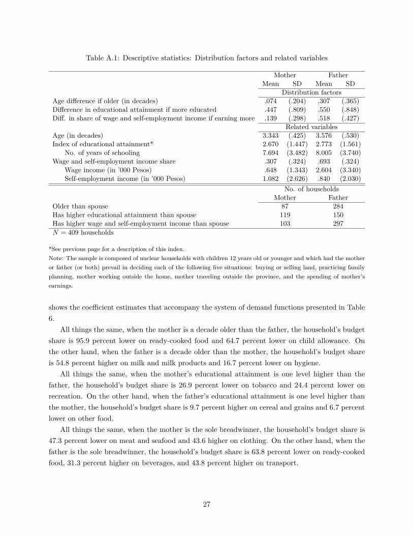
Table A.1: Descriptive statistics: Distribution factors and related variables

Mother Father Mean SD Mean SD

Distribution factors Age difference if older (in decades) .074 (.204) .307 (.365) Difference in educational attainment if more educated .447 (.809) .550 (.848) Diff. in share of wage and self-employment income if earning more .139 (.298) .518 (.427)

Related variables Age (in decades) 3.343 (.425) 3.576 (.530) Index of educational attainment* 2.670 (1.447) 2.773 (1.561)

No. of years of schooling 7.694 (3.482) 8.005 (3.740) Wage and self-employment income share .307 (.324) .693 (.324)

Wage income (in ’000 Pesos) .648 (1.343) 2.604 (3.340) Self-employment income (in ’000 Pesos) 1.082 (2.626) .840 (2.030)

No. of households Mother Father

Older than spouse 87 284 Has higher educational attainment than spouse 119 150 Has higher wage and self-employment income than spouse 103 297 N = 409 households

*See previous page for a description of this index. Note: The sample is composed of nuclear households with children 12 years old or younger and which had the mother

or father (or both) prevail in deciding each of the following five situations: buying or selling land, practicing family

planning, mother working outside the home, mother traveling outside the province, and the spending of mother’s

earnings.

shows the coefficient estimates that accompany the system of demand functions presented in Table

6. All things the same, when the mother is a decade older than the father, the household’s budget

share is 95.9 percent lower on ready-cooked food and 64.7 percent lower on child allowance. On

the other hand, when the father is a decade older than the mother, the household’s budget share

is 54.8 percent higher on milk and milk products and 16.7 percent lower on hygiene. All things the same, when the mother’s educational attainment is one level higher than the

father, the household’s budget share is 26.9 percent lower on tobacco and 24.4 percent lower on

recreation. On the other hand, when the father’s educational attainment is one level higher than

the mother, the household’s budget share is 9.7 percent higher on cereal and grains and 6.7 percent

lower on other food. All things the same, when the mother is the sole breadwinner, the household’s budget share is

47.3 percent lower on meat and seafood and 43.6 higher on clothing. On the other hand, when the

father is the sole breadwinner, the household’s budget share is 63.8 percent lower on ready-cooked

food, 31.3 percent higher on beverages, and 43.8 percent higher on transport.

27

Table A.2: Demand for consumption goods as a function of decision-making arrangement and distribution factors (Basic set of controls included) Dependent variable Independent variables

Age difference Difference in Diff. in share of wage if older educ’l attainment and self-employment

Log consumption (in decades) if more educated income if earning more expenditure share in: Mother Father Mother Father Mother Father

Cereal and grains .004 −.102 .070+ .097* −.150 −.003 (.166) (.119) (.049) (.056) (.173) (.091)

Meat and seafood −.078 .134 .006 −.045 −.473* .108 (.285) (.205) (.065) (.068) (.256) (.102)

Milk and milk products .085 .548*** −.214 −.045 .097 .262 (.516) (.206) (.149) (.168) (.278) (.265)

Vegetables and fruits −.471 .161 −.060 −.043 .120 .134 (.360) (.151) (.102) (.092) (.176) (.140)

Ready-cooked food −.959* −.154 .221 .150 −.043 −.638** (.546) (.319) (.160) (.146) (.314) (.298)

Other food −.091 .048 −.037 −.067** −.108 .059 (.108) (.070) (.039) (.026) (.119) (.073)

Beverages −.277 .102 −.070 −.058 .220 .313* (.378) (.156) (.079) (.080) (.161) (.175)

Alcohol .217 .075 −.060 −.218 −.026 −.201 (.525) (.297) (.156) (.160) (.368) (.298)

Tobacco −.558 −.010 −.269* −.118 .350 −.021 (.573) (.423) (.152) (.149) (.386) (.318)

Transport .140 .209 −.085 −.002 .372+ .438** (.450) (.212) (.126) (.109) (.258) (.222)

Hygiene .041 −.167** .033 .052 −.052 −.020 (.132) (.077) (.038) (.044) (.088) (.061)

Clothing −.080 .007 .150+ .108 .436* −.132 (.415) (.221) (.094) (.094) (.227) (.171)

Medicine .081 .026 −.024 .118 −.159 −.028 (.392) (.188) (.127) (.110) (.272) (.178)

Child allowance −.647** −.128 −.161+ −.030 −.179 −.180 (.327) (.165) (.101) (.091) (.213) (.181)

Schooling −.123 .111 −.048 −.106+ −.002 .028 (.274) (.182) (.081) (.067) (.108) (.128)

Recreation .558 −.025 −.244* −.009 .626+ .141 (.457) (.276) (.128) (.102) (.425) (.303)

N = 409 households Note: The table presents IV coefficient estimates and standard errors from a SUR, with disturbance terms clustered at the village level and allowed to be correlated across equations. The excluded IVs for (log) total household consumption expenditure are (log) total household income and in-kind transfers received. The set of basic controls used is listed in Table 4. Significance indicated at the following confidence levels: + 85 percent; * 90 percent; ** 95 percent; *** 99 percent.

28

B Village-level wages and prices

In the CLHNS community questionnaire, data on prevailing wage rates for seven different occupations were obtained from two knowledgeable persons (community leader/councilor, school principal, teacher, etc.) in each village, and the wage rates were allowed to have different units (per piece, daily, daily with free meal, weekly, or monthly45). For price data, six knowledgeable persons were

asked to identify the two most frequented markets or store for four different food categories, and

then prices on 19 goods were obtained from these two stores, with different units (including local sizes that are not easily convertible) depending on what the store actually had for sale. In both

cases, missing entries were prevalent. To limit the problem of arbitrary sample selection,46 I used

all of the different wage rates and prices, listed below, using the most common units mentioned for

each, and using the average value if two sources were available. I also included dummy variables

denoting missing entries (either due to the use of a different unit or actual missingness) for each

wage or price.47

Occupations with wage rate information

• Unskilled wage labor in poblacion or city, government or private

• Unskilled farm labor

• Yaya (domestic helper whose primary responsibility is taking care of children)

• Other domestic helper

• Construction worker

• Cargador (stevedore)

• Cosmetologist (barber or hairstylist)

Goods with price information

• Rice (wagwag, first class)

• Corn grits (#14)

• Pork (pure meat, no bones)

• Beef

• Chicken

• Eggs, medium

45It was unclear how weekly and monthly rates could be converted into daily rates since using the usual numbers resulted in wages that don’t line up well with the reported daily rates for other villages.

46One possibility was to use variables with the least number of missing entries, and then use casewise deletion to drop observations. This was unsatisfactory because one would have to make choices about which variables to keep (sometimes, the more important items had more missing entries), and casewise deletion would lead to a further reduction in the sample size.

47The average wage or price for the whole sample was substituted into the corresponding missing entries for each variable.

29

• Bananas (lakatan, second class, small)

• Bananas (latundan, second class, small)

• Tomato (native, small)

• Cabbage

• Evaporated milk (cheapest brand, small)

• Condensed milk (cheapest brand, large)

• Powdered milk (cheapest brand, small)

• Infant formula (cheapest brand, small)

• Edible oil

• Salt (solar-evaporated, unrefined)

• Gasoline

• Kerosene

• Cement

C Variable list

Components of consumption expenditure categories

• Cereal and grains: rice, corn, flour; cassava, sweet potato, potato, yam; bread, crackers, noodles, pasta

• Meat and seafood: beef, pork, chicken, goat, intestines, liver or gizzard, frozen or canned

meat; fresh fish, dried fish, smoked fish, canned fish, salted fish, shrimps and other shellfish

• Milk and milk products: fresh milk, evaporated milk, condensed milk, powdered milk, cheese, butter

• Vegetable and fruits: swamp cabbage and other leafy vegetables, green beans, onions, tomatoes, carrots, cucumber; mango, banana, papaya, guava, pineapple, apple, pomelo; peanuts, mung beans, soy beans, green peas

• Ready-cooked food: gruel, meatballs, salad, mung beans, noodles

• Other food: chicken egg, duck egg, quail egg; oil, margarine; salt, pepper, ketchup, fish sauce, vinegar, sugar

• Beverages: tea, coffee, cocoa or native chocolate, juices, softdrinks

• Alcohol: beer, palm wine, rum, gin

• Tobacco: cigarettes, abano

• Transport: public transport, gasoline, vehicle maintenance

30

• Hygiene: laundry detergent, bath soap, toothpaste, toilet paper, cosmetics

• Clothing: clothes, shoes, socks, hats, accessories

• Medicine (medical expenditures): hospital, health center, doctor, traditional midwife, traditional healer

• Child allowance

• Schooling (educational expenditures): enrollment, matriculation/tuition fee, Parents and

Teachers Association, Boy/Girl Scouts, vocational course, school materials, books, uniforms

• Recreation: newspapers, magazines; movies

D Results with village-level fixed effects

Table A.3: Group statistics for village-level fixed effects estimation Cumu-

Village lative sample No. of no. of

size villages groups

29 1 1

N = 409 households

28 1 2 22 1 3 19 1 4 18 1 5 16 1 6 15 1 7 14 3 10 12 2 12 11 1 13 9 3 16 8 2 18 7 3 21 6 1 22 5 1 23 4 2 25 3 9 34 2 15 49 1 45 94

31

Table A.4: Demand for consumption goods as a function of decision-making arrangement, Estimates with distribution factors and village-level fixed effects


arrangement index consumption Controls Log consumption Joint relative to: expenditure Basic Additional expenditure share in: Mother Father (instrumented) set DF FE

Cereal and grains .203+ .262 −1.086*** Yes Yes Yes (.137) (.187) (.281)

Meat and seafood −.324 −.249 .274 Yes Yes Yes (.253) (.222) (.218)

Milk and milk products .783* .469 1.514** Yes Yes Yes (.403) (.444) (.598)

Vegetables and fruits −.206 −.110 .710* Yes Yes Yes (.332) (.233) (.419)

Ready-cooked food .121 −.007 −.865+ Yes Yes Yes (.343) (.401) (.560)

Other food −.120 −.085 −.290** Yes Yes Yes (.108) (.122) (.143)

Beverages .030 −.539** 1.537*** Yes Yes Yes (.191) (.211) (.308)

Alcohol .315 −.478 −1.180* Yes Yes Yes (.397) (.454) (.640)

Tobacco .222 −.510 .119 Yes Yes Yes (.380) (.439) (.821)

Transport −.314 .324 .601 Yes Yes Yes (.292) (.392) (.524)

Hygiene −.107 .011 −.468*** Yes Yes Yes (.123) (.120) (.175)

Clothing .155 .051 1.653** Yes Yes Yes (.282) (.359) (.654)

Medicine .308 .290 .220 Yes Yes Yes (.350) (.325) (.595)

Child allowance −.054 −.003 .236 Yes Yes Yes (.212) (.174) (.415)

Schooling .048 −.034 .610* Yes Yes Yes (.238) (.207) (.320)

Recreation −.122 −.109 2.320*** Yes Yes Yes (.383) (.381) (.639)


Note: The table presents IV coefficient estimates and standard errors from a SUR, with disturbance terms clustered at the village level and allowed to be correlated across equations. The excluded IVs for (log) total household consumption expenditure are (log) total household income and in-kind transfers received. The set of basic controls used is listed in Table 4; additional controls for distribution factors (DF) are described in Appendix A, while FEs are village-level fixed effects. Significance indicated at the following confidence levels: + 85 percent; * 90 percent; ** 95 percent; *** 99 percent.

32

Documents

November 11, 2011 - PacDev 2018 at UC Davis - About the ... Is couple’s joint decision making associated with favorable household consumption patterns for children? Evidence from