Embed Size (px)
Citation preview
SOFT BODY IMPACT OF CANTILEVER BEAMS.(U)MAR S0 J D SHARP
N CLASSIFIED AFML-TR-79169 NL
mmh"hllhmlhlhluBBBBhBBhmBhBBlEEEIIIIIIIIIIEIIIIIIIIIII-

t 1 . 1111122
OO 136 IIIIIT
111111.25 1111.4 111111.6
MfEROCOPY RESOLUTI(%, USI CIIARINAINA I' M \I W I IA~NPAR\I'l '

AFML-TR-79-4169
SOFT BODY IMPACT OF CANTILEVER BEAMS
Jeffry D. SharpI Metals Behavior Branch
Metals and Ceramics Division
March 1980
TECHNICAL REPORT AFML-TR-79-4169
Interim Report for Period October 1977)- uly 1979
Approved for public release distribution unlimited.
*DTIC,.-- :LECTEDAIR FORCE MATERIALS LABORATORY A CTAIR FORCE WRIGHT AERONAUTICAL LABORATORIES JUN 2 5 1980AIR FORCE SYSTEMS COMMANDWRIGHT-PATTERSON AIR FORCE BASE, OHIO 45433 B
80 6 23 106..., ..,..,,.. . ..

a
NOTICE
When Gdvernment drawings, specifications, or other data are used for any pur-pose other than in connection with a definitely related Government procurementoperation, the United States Government thereby incurs no responsibility nor anyobligation whatsoever; and the fact that the government may have formulated,furnished, or in any way supplied the said drawings, specifications, or otherdata, is not to be regarded by implication or otherwise as in any manner licen-sing the holder or any other person or corporation, or conveying any rights orpermission to manufacture, use, or sell any patented invention that may in anyway be related thereto.
This report has been reviewed by the Information Office (O) and is releasableto the National Technical Information Service (NTIS). At NTIS, it will be avail-able to the general public, including foreign nations.
This technical report has been reviewed and is approved for publication.
THEODORE NICHOLAS NATHAN G. TUPPE*" ChiefProject Engineer Metals Behavior BranchMetals Behavior Branch Metals and Ceramics DivisionMetals and Ceramics Division
"If your address has changed, if you wish to be removed from our mailing list,or if the addressee is no longer employed by your organization please notifyAFWAL/MLLN ,N-PAFB, OH 45433 to help us maintain a current mailing list".
Copies of this report should not be returned unless return is required by se-curity considerations, contractual obligations, or notice on a specific document.
AIR FORCE/56780/18 June 1980 -400

SECURITY CLASSIFICATION Of THIS PAGE (Ma.n. Dat. Enterod), EDISRCIN
jOFT BODY IMPACT OF CANTILEVER B EAI4' Oct 277-Julg 3979
JfrD.SapIn-House d.--IL -r
. DISTRIUTIORNATIEN NAME AND1 AeDRES .POIIAf RJC.TS
AFpprved fonpulica rLbasetribuio unlimited.
I1. SUPPRLLENTAR OESNMNDRS
Aoft odye Naeilaormalor ModesajaAn rtilerone am DyamicrtresonFs
20. ABTRCT Cotneoreee d Ifnc eay in ti ng yfbl c e) 1. EU
Aprods f paricurla distrisuthen responsedo. tucueipatdb
Soft Body, suhasabrd.l Asoadesulefrshv enmd ntelsseveraler yea touDrtn hynamic bepn ehairo ld-iesrcue ne
Impact
Vibration
20-BTAT(otneo ees ieI eesr an & i et ify b blok nutbow

SSC[CUPAITY CLASSIFICATION OF THIS PAGl[("fan Data ENoemd)l
investigated as thoroughly. This study experimentally and analytically
investigates the stress/time response of a cantilever beam subjected toimpact loading from a soft object. Results from several differentanalytical models employing the Euler-Bernoulli Beam Theory are compared toexperimental data, and the validity of each model is assessed. The effectsof structural damping, beam dimensions and the Timoshenko Theory parametersare discussed and conclusions as to their importance are drawn. It was deter-mined that a cantilever beam impacted by a soft body can be accuratelymodeled as a forced vibration problem using the Euler-Bernoulli Theory andlinear modal analysis with damping. In addition, it was shown that largestructures can be linearly scaled down for impact testing without affectingthe results.
SECURITf CL&SSIICATIOU OF r, PAGC(fWtsn Date Entiefd)

AFML-TR-79-4169
FOREWORD
This work reported herein performed at the Metals Behavior Branch,
Metals and Ceramics Division, Air Force Materials Laboratory. The work
was performed under in-house Project No. 241803, "Dynamic Behavior of
Engine Materials." The work was conducted by Mr. Jeffry D. Sharp,
collocated from ASD/ENFSM, Wright-Patterson AFB, Ohio.
The author would like to offer thanks to his thesis advisor,
Dr. George Sutherland, Ohio State University, for his suggestions and
guidance throughout this work, to Dr. Theodore Nicholas, AFML/LLN, for
making available the experimental facilities and providing technical advice,
and to Ms. Barbara Lear, ASD/ENF for her secretarial assistance.
The research was conducted during the period October_]9 7 to
July 1979. This report was submitted for publication in September 1979.
I, .-Ici;TL
iJ '4_-c e
; a
iii
1i. )X :td
AFML-TR-79-4169
TABLE OF CONTENTS
SECTION PAGE
I INTRODUCTION 1
II EXPERIMENTAL PROCEDURE AND RESULTS 2
III THEORETICAL SOLUTION 20
IV NUMERICAL ANALYSIS AND RESULTS 31
V COMPARISON OF EXPERIMENTAL AND THEORETICAL RESULTS 37
VI DISCUSSION AND CONCLUSIONS 46
APPENDIX A ESTIMATION OF PROJECTILE VELOCITY 49
APPENDIX B STRAIN IN LINEARLY SCALED BEANS 51
APPENDIX C EVALUATION OF TIMOSHENKO BEAM THEORYEFFECTS 53
APPENDIX D NUMERICAL STABILITY 55
APPENDIX E LISTING OF COMPUTER PROGRAM 57
REFERENCES 67
t9
bV
h
- *" i i i- '' -"
..

AFML-TR-79-4169
LIST OF ILLUSTRATIONS
FIGURE PAGE
1 Schematic of Cantilever Beam Specimens 3
2 Strain Gage Placement on Beams 4
3 Beam Specimen Mounting Configuration 6
4 Experimental Strain at Root Location 8
5 Experimental Strain at Impact Location 10
6 Experimental Strain in 14.0 Inch Beam (5.0 Ms.) 12
7 Experimental Strain in 14.0 Inch Beam (0.5 ms.) 13
8 Experimental Strain in 14.0 Inch Beam (500 ms.) 14
9 Fourier Transforms of Root Strain Data 15
10 Fourier Transforms of Impact Site Strain Data 17
11 Schematic of Initial Velocity Models 22
12 Schematic of Forced Vibration Models 26
13 Example of Computer Input/Output 32
14 Example of Computer Generated Strain vs. Time Plot 33
15 Strain at Root of 5.6 Inch Beam From ForcedVibration Models 39
16 Strain in 14.0 Inch Beam From Step FunctionModel (5.0 ms.) 40
17 Strain in 14.0 Inch Beam From Half-Sine WaveModel (5.0 ms.) 42
18 Strain in 14.0 Inch Beam From Step FunctionModel (0.5 ms.) 44
C-1 Shear Effects in Cantilever Beam Vibration 54
vi

AFML-TR-79-4169
LIST OF TABLES
TABLE PAGE
I Experimental Results 19
2 Theoretical Results Without Damping 35
3 Theoretical Results With Damping 36
4 Comparison of Experimental and Theoretical Results 38
5 Comparison of Experimental and Theoretical ResultsWith Damping 38
i
?; v i i

AFML-TR-79-4169
LIST OF SYMBOLS
Dp Diameter of Projectile; in.
Pp Density of Projectile; lbm/In.3
V Velocity of Projectile; fps
M Mass of Projectile; lbmp
PB Density of Beam; lbm/in.3
AB Cross-Sectional Area of Beam; in.2
MB Mass of Beam
t Length of Beam; in.
E Modulus of Elasticity of Beam; lbf/In.2
I Moment of Inertia of Beam Cross Section; in.4
L Spanwise Location of Impact; in.
T 0 Duration of Impact; sec.
*(x) Mode Shape Function for Cantilever Beam; In.
Modal Damping Factor
e Strain; in./in.
viii

AFML-TR-79-4169
SUMMARY
With thrust-to-weight ratios in aircraft gas turbine engines
increasing, all components are required to operate at higher steady-
stress levels. This situation, coupled with cyclic life limits based
on crack propagation, demands a better understanding of the operating
environment and various loading conditions to which a component may be
subjected throughout its useful life. Vibratory stresses induced in
rotating airfoils by toreign object impacts are a real part of jet
engine operating environments and require careful consideration when
designing high performance blades. However, before one can analyze
a component for such conditions, the loading mechanism must be under-
stood. This has been investigated for members of similar stiffnesses
impacting each other (References 1 through 4), but little work has been
done to define and analyze the effect of a soft body impacting a member
with the approximate geometry and stiffness of a fan blade. The first
step toward accomplishing this understanding is to fabricate several
cantilever beam test specimens, impact them with soft projectiles, and
record the strain response at various locations as a function of time.
From this data base, a simple beam theory model can be evaluated for
several different cases, each treating the impact as a slightly dif-
ferent phenomenon, but based on the common assumption that all the
projectile momentum is transferred to the beam. The results indicate
that a soft-body impact on a cantilever beam can be modeled as forced
vibration for the duration of the impact, then free vibration for all
time thereafter. The forcing function created by the projectile is
best modeled as a step-function distributed over an area. Damping in
the system has a significant effect on strain in the beam, but is dif-
ficult to accurately predict, and thus should not be considered in
maximum strain calculations. However, an accurate strain/time history
can be predicted if modal damping values for the first four resonant
modes are known. Impact testing of very large structures can be performed
on scaled down models with no change in results.
ix

AFNL-TR-79-4169
SECTION I
INTRODUCTION
The problem of predicting the response of a blade-like structure to
an impact by a soft body is very complex and involves many structural
interactions. To begin analyzing all the load transfer mechanisms
present in such a problem is a monumental task. One must initially take
a more basic approach. The objective of this study is to determine how
a simple cantilever beam responds to an impact on its centerline by a
soft object. If the overall bending strain at various spanwise locations
in a beam can be recorded throughout an impact, the gross loading
mechanism can be studied and an analytical model can be developed to
predict the response.
To accomplish this objective, four geometrically similar beams were
fabricated and instrumented with strain gages at various spanwise loca-
tions, mounted in a cantilever configuration, and impacted with geomet-
rically similar soft projectiles. Data from the strain gages was
digitally recorded during impact, stored, then analyzed to determine
maximum strain at each gage location and the modal content of each
response. Any damping effects present were noted. This provided the
dynamic response data necessary to evaluate several proposed analytical
models.
Next, analytical models based on the Euler-Bernoulli Beam Theory and
employing linear modal analysis were formulated. Two basic approaches
were used to simulate the impact loading. The first was to assume a
purely impulsive loading in which the projectile imparted an instan-
taneous initial velocity to the beam. The second treated the impact as
a forced vibration problem, which modeled the impact as a.) a step
function and b.) a half sine wave in time. Each model was defined andformulated on a computer and the resulting time responses were compared
with the test data to determine its accuracy. The following text
describes in detail the experimental work performed, the data analysis
techniques used, the different model derivations and formulations, and
finally, the results obtained from each model and a comparison with
experimental results.
I

AFML-TR-79-4169
SECTION II
EXPERIMENTAL PROCEDURE AND RESULTS
Four cantilever beam specimens were fabricated from 7075 T-6
aluminum, approximately 91 R or 190 B hardness, the smallest beam being
5.6 inches long, 1.2 inches wide, and 0.15 inches thick. The remaining
beams were scaled from these dimensions by factors of 1.5, 2.0, and 2.5.
To ensure cantilever boundary conditions and minimize damping effects
from mounting fixtures, the root section of each specimen was left
significantly thicker than the rest of the beam, as shown in Figure 1.
For simplicity, the impact site of each beam was chosen to be at
75% span. This provided a reasonable portion on either side of thedesired impact location to ensure contact by the whole projectile.
Strain gages were mounted on each beam at the root and 75% span on the
side opposite that to be impacted. On three of the four beams, gages
were also placed at 25% and 50% span to record additional data (Figure 2).
These four locations were chosen to help identify the location of
maximum strain and to provide a sufficient amount of strain/time history
information to facilitate verification of analytical models.
The projectiles used to impact each beam were spherical bodies of
micro-balloon gelatin, a porous gelatin used to simulate bird impacts
(Reference 7). Projectile sizes and velocities were selected to meet
several criteria. The base line projectile diameter was chosen to be
0.5 inches so it would be small compared to the smallest beam length
and width. The geometric ratios used to size the beams were also used
to determine the remaining projectile diameters. This calculation
yielded projectile diameters of 0.5, 0.75, 1.0, and 1.25 inches.However, a 0.75 inch diameter mold was not available, so the projectile
sizes actually used for the impact experiments were 0.5, 0.70, 1.0, and
1.25 inches in diameter. A calculation was made for approximating
projectile velocities based on a one degree-of-freedom lumped mass
beam model (Reference 6). To assure elastic response, velocity calcula-
tions were based on 0.25% strain at the beam root, which predicted aprojectile velocity of about 570 fps. These calculations are detailed
2

I
AFML-TR-79-4169
7075 T-6
THICKENED ROOTSECTION
MOUNT ING-BOLT0 _- HOLES
Figure 1. Schematic of Cantilever Beam Specimens
3
- 4

AFML-TR-79-41 69
A - ROOT LOCATION:ALL BEAMS
B - 25% SPAN; 5.6,11.2, & 14.0
C - 50% SPAN; 5.6,11 .2, & 14.0
D - 75% SPAN: ALLBEAMS
A
00
Figure 2. Strain Gage Placement on Beams
4

AFML-TR-79-4169
in Appendix A. To account for the gross model used, the velocity
prediction was decreased to 400 fps. An attempt was made to maintain
this projectile velocity for each beam specimen so the concept of
scaling impact specimens could be investigated.
Two different devices were used to record transient strain data.
A Hewlett-Packard 5451B Fast Fourier Analyzer (FFT) capable of
digitizing and storing four channels of data at 20 KHZ was employed to
provide a record of transient response data which could be analyzed at
a later time. A Zonics AE 102-2 transient recorder capable of digitizing
eight channels of data from 2 KHZ to 200 KHZ was utilized to investigate
short time and long time responses. Strain data recorded by the FFT unit
was stored on a magnetic disk, while the transient recorder data was
stored temporarily in the recorder and then input to an oscilloscope and
photographed.
For testing, each beam was mounted in a steel fixture as shown in
Figure 3. The entire assembly was then placed inside a steel enclosure
on the impact range, positioned with a laser aiming device and then
secured to the enclosure.
Projectiles were first weighed and the weight recorded, and then
launched from a smooth-bore tube, propelled by compressed air, compressed
helium, or burning gunpowder. Each projectile was carried down the
tube in a sabot, a plastic bore fitting carrier, which protected it
from the launch tube walls. Several inches in front of the target a
constriction in the barrel stopped the sabot, allowing the projectile
to continue. Before striking the beam, the projectile tripped a pair of
laser light sources connected to a time interval counter to measure its
velocity.
Several shots were made at each beam to "zero in" on the amount of
pressure/powder necessary to attain the desired velocity. Impacts on
the first beam indicated that a velocity between 300 and 350 fps was
adequate to produce the desired strain at the specimen root. Thus,
those values became bounds on the desired velocity for all remaining tests.
5

AFML-TR-79-4169
I--
4-
A A 0
LA LAI I I I
I t II I II,
U
6-E
I H IH I
LAL

AFML-TR-79-4169
Figures 4A through 4D are strain/time responses from each beam root
location. Variations in peak strain values due to differing projectile
velocities and densities can be seen. The data indicates, however, that
linear scaling of all beam and projectile dimensions will produce equal
strains. Appendix B is a dimensional analysis that supports this
observation. Responses from the impact site (75% span) on each beam
are shown in Figures 5A through 5C. The same observations made of the
root strain data can also be made of these traces. In addition, very
little damping effect can be observed in either set of data, except at
high frequency. Figures 6A through 6D are the strain responses from each
gage location on the 14.0 inch beam. These traces indicate that the
maximum strain experienced during impact occurs at the beam root.
Figures 7A through 7D show the response of the 14.0 inch beam over 0.5
milliseconds as being slow and containing no high frequency components.
Figures 8A through 8D are the responses of the same locations over 500
milliseconds, demonstrating damping in the system affecting only long-
term response. All the strain traces indicate the presence of several
frequency components. However, it should be noted that the sampling rate
used to record this data was too slow to pick up frequencies above the
first or second mode. Figures 9A through 9D are Digital Fourier Trans-
forms of root strain responses from each beam, showing the presence of
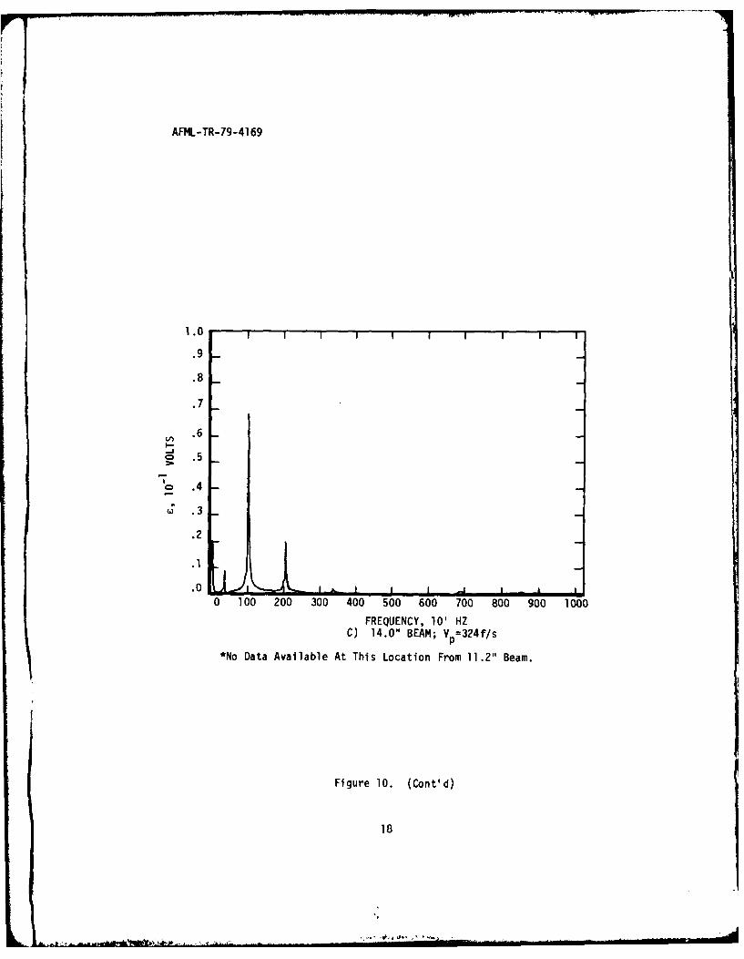
the first four beam bending modes. Similar plots for the 75% span
location, Figures lOA through 10C show the same result with a small
contribution from the fifth mode. Table 1 summarizes the maximum strain
values from all experimental records.
An overview of the test results leads to several conclusions. The
maximum stress over the entire impact event occurs at the beam root.
For the same projectile velocity and density, linearly scaled beams and
projectiles will produce the same impact strain values. The strain
response at any location in the beam has significant contribution from
only the first five resonant bending modes. Damping in the system has
little effect on the peak strain value but does become apparent in long
time response. These results provided the basis for evaluating several
analytical models.
7

AFM4L-TR-79-41 69
1.0 I
.8
.6
.4
.2
.0
-.
C:-.4
-.6
-.8
-1.0 I
0 500 1000 1500 2000 2500 3000 3500 4000 4500 5000
Time, 10O5sec.A) 5.6" Beam; V =341f/s
1 .0
.8
.6
.4
.2
I.2
-. 4
-.6V V
-. 8
0 500 1000 1500 2000 2500 3000 3500 4000 4500 5000Time, 10O5sec.
B) 8.4"1 Beam; V =336 f/s
Figure 4. Experimental Strain at Root Location
8A

AFM4L-TR-79-41 69
2.0
1.6
1.2
.8
.4
--.8
-1.2
-1 .6
-2.0L0 500 1000 1500 2000 2500 3000 3500 4000 4500 5000
Time, 0O-5 secC) 11.2" Beam; V =330f/s
1 .01
.8
.6
.4
.2
.4
-.6
-.8
0 500 1000 1500 2000 2500 3000 3500 4000 4500 5000
Tme, -O5 sec0) 14.0" Beam; V =324f/s
Figure 4. (Contd)
9

AFML-TR-79-41 69
5.0
4.0
3.0
2.0
1.0
00
-1.0
-2.0
- 3.0
-4.0
0 500 1000 1500 2000 2500 3000 3500 4000 4500 5000
Time, l05 secA) 5.6"1 Beam; V =341f/s
5.0
4.0
3.0
2.0
1.0
-J.0
.- -1.0
-2.0
-3.0
-4.0
-5.0 a0 500 1000 1500 2000 2500 3000 3500 4000 4500 5000
Time, 10-5secB) 8.4"1 Beam; V =336f/s
Figure 5. Experimental Strain at Impact Location
10

AFML-TR-79-41 69
5.0
4.0
3.0
2.0
1.0
o) .0
'CD -1.0
J -2.0
-3.0
-4.0
-5.0 I0 500 1000 1500 2000 2500 3000 3500 4000 4500 5000
Time, lO-5secC) 14.0" Beam; V =324f/s
Figure 5. (Cantd)
*No Data Available At This Location From 11.2" Beam.
L i1

AFML-TR-79-41 69
on 0
.- ' CDJ 'o
(N -F0
Q- E
C3 @CL
LA U
00
cJ CDuo
LnL
LA-0
otN 0 0I 3
u.
-- %0C
00 EU 0; C
S110 LAO 12 - 1.

AFML-TR-79-4169v) .UM
0 0i
C; CDI inU
4. . , ,.oZ 0
-. ,,N S=
" +- H -- H - "U
-- N ale
o 0 -
- -- - - - - n co
- a,
CD Co C5 ID CD. DC ; C
So 0',0 * D
II
I I I I I I _-
SI1IOA '3 1 SI'IOA '3 c
, )
cla,ILO
CD 0 DC )C
- -- - - - - - - - - --0A- -'3 3aO '

AFML-TR-79-4169
o o
0 L0
CDC%o a. c,',-
" 'J" l ilE
..... ... .... .... .... O). 0o 0"
- 0 r"
•~C CDlIA
-- _- o - . o E"- ! - - - 19 r.to Co CsJ C o C> £0 CD'U C.J C3J Co t
I I I I I I
SIIOA '3 SI1OA '3
CD%CD L 0
Ln,
CL'U
0D C
o0
.. ... .. . . .. t
o Ln
CD~ CD~
L
19 $4 It ~ s~s a I+4-$H+I1+!H4H!4t %9
to CD CD C5 C D 14 o C> CD C D Cu CD C
o IO '3 0 0 014 0 0 0 0 0

AFM4L-TR-79-41 b9
2.0
1.8
1.6
1.4
g~1.2-D
S 1.0
' .6
.4
.2
.0AL - -I0 100 200 300 400 500 600 700 800 900 1000
FREQUENCY, 10 HZA) 5.6" BEAM; V =341 f/s
5.0
4.5
4.0[
3.5
3.0 -
~2.5
2.0
~1.5
1.0
.5
.0 , -- I
0 500 1000 1500 2000 2500 3000 3500 4000 4500 5000FREQUENCY, HZ
B) 8.4" BEAM; V =336f/s
Figure 9. Fourier Transforms of Root Strain Data
15

AFML-TR-79-4169
5.0
4.5
4.0
-. 3.5
3.0
2.5
2.0
1.5
1.0
.5
.0 -.0 100 200 300 400 500 600 700 800 900 1000
FREQUENCY, 10 HZC) 5.6" BEAM: Vp=341f/s
2.0 I
1.8
1.6
1.4
1.2I,-
o 1.0
'- .8
".6
.4
.2
0 00 200 300 400 500 600 700 800 900 1000
FREQUENCY, HZD) 8.4" BEAM: Vp=336f/s
Figure 9. (Cont'd)
16

AFM4L-TR-79-4 169
5.0
4.54.0
U3.5
'2.5
.2.0
1.5
1.0
.5
.0 L4LIIIII0 100 200 300 400 500 600 700 800 900 1000
FREQUENCY, 101 HZA) 5.6" BEAM; V =341 f/s
1.0
.9
.8
.7
.5
-.4
.3
.2
.1
.00 500 1000 1500 2000 2500 3000 3500 4000 4500 5000
FREQUENCY, HZB) 8.4" BEAM; V =336f/s
Figure 10. Fourier Transforms of Impact Site Strain Data
17
AFML-TR-79-41 69
1.0 r
.9
.8
.7
V) .6-
o .5
oc .4
() .3
.2
.1
.0 j0 100 200 300 400 500 600 700 800 900 1000
FREQUENCY, 10' HZC) 14.0" BEAM; V =324f/s
*No Data Available At This Location From 11.2" Beam.
Figure 10. (Cont'd)
18

AFML-TR-79-4169
TABLE 1
EXPERIMENTAL RESULTS*
Beam Length,inD_ in Vp, f/scroot, %E25 50max ES
5.6 0.5 370 0.278 - - 0.155 1.5
5.6 0.5 341 0.269 _ _0.113 0.3**
8.4 0.7 344 0.225 0.134 2.1
8.4 0.7 336 0.231 - 0.103 2.1
11.2 1.0 366 0.282 - - 0.139 2.9
14.0 1.25 365 0.247 0.162 j 0.116 0.147 3.55
14.0*** 1.25 343 0.209 0.154 0.077 g 0.116 5.0
14.0 1.25 324 0.250 - 0.091 0.114 2.3
14.0 1.25i 317 0.254 0.175 0.086 0.105 3.0
* Strains are absolute value.
** Recorder triggered late.
* Large data point separation; poor strain resolution.
19

AFML-TR-79-4169
SECTION III
THEORETICAL SOLUTION
Two basic approaches were taken to modeling the soft-body impact
problem. The first entailed treating the projectile as imparting an
initial velocity to the beam at the point of impact. This approach was
suggested in Reference 9 and applied to a hard-body impact problem in
Reference 8. The second approach was to treat the beam response to
impact as a forced vibration, as in Reference 4. The forcing function
was modeled as both a square wave and a half-sine wave. In both
formulations, the common assumption made was that all the projectile
momentum is transferred to the beam, i.e., linear momentum is conserved
and the projectile assumes a velocity of zero after impact. This
assumption, which is supported in Reference 7 and by experimental
observation, implies that the coefficient of restitution is close to
zero, but unknown. Both formulations are based on linear modal theory
and employ the Euler-Bernoulli beam relationships. Timoshenko beam
effects (i.e., shear and rotary inertia) were investigated and found to
be negligible (Appendix C).
The solution for free vibration of a beam developed in Reference 5
was used to determine the resonant frequencies and mode shapes of a
cantilever. The general beam mode shape (as a function of space
coordinate only) is given by:
y(x) = A sinh(Px) + B cosh(ax) + C sin(ax) + D cos(fx) (1)
where 8 is dependent upon the applied boundary conditions. For a
cantilever:
y-O
at x - 0dy/dx = 0
M - 0 or d2y/dx2 = 0at x t
V - 0 or d3 y/dx3 - 0
20

AFML-TR-79-4169
Substitution of these boundary conditions into Equation 1 yields:
cosh(OZ)cos(B) + 1 - 0 (2)
which is the solution for ab for the various resonant modes. The mode
shape expression can also be rewritten, as a result of applying the
boundary conditions, as:
y(x) = A {cosh(Bx) - cos(Bx) - K [sinh(ax) - sin(x)]} (3)
where k = sinh(OZ) - sin(sk)/cosh(at) + cos(8L). For simplicity,
Equation 3 will be written as:
y(x) = A O(x)
defining
O(x) = cosh(8x) - cos(Sx) - K [sinh(ax) - sin(Bx)] (3a)
Employing linear modal theory, the total response of the beam, including
time variation, can be formulated as:
N = I ANON(X)N(t)
with ON(X) corresponding to a solution of Equation 3a for a particular
value of 8, determined from Equation 2. TN(t) is a time varying function
of the resonant frequency for each mode, wN, calculated from
/2N El/pA (5)
Assuming a sinusoidal time response,
TN(t) = C1 sin(OBt) + C2 cos("Nt) (6)
CI and C2 are determined by evaluating the initial conditions of the
problem. At this point, each approach to analyzing the soft body impact
must be treated separately.
1. INITIAL VELOCITY SOLUTION
The first approach taken was to assume the projectile imparts an
initial velocity to the beam, as shown pictorially in Figure llA. The
velocity can be expressed as:
V - V6(x - L) (7)
21

AFML-TR-79-41 69
Compatibility: M p Vp = 0 pBAB;(x, O)dx
y(L, 0) -6( L)
Y(O, t) =0
y.(O, t) =0
A) Initial Velocity at a Point
I(L, 0) V{U(x -L + D/2) -
U(x - L -D/2)}
M - Compatibility: MVA
y(O, t) =0Cy'(O, t) 0
B) Initial Velocity Over an Area
Figure 11. Schematic of Initial Velocity Models
22

AFML-TR-79-4169
At time t = 0, the initial conditions are:
y(x, 0) - 0
'(x, 0) - VS(x - L)
Application of the I.C.s yields C2 = 0 and
V (x - L) - N 1 A,%ON(X) (8)
Multiplying both sides by a particular mode shape, OM(x), applying
orthogonality conditions and integrating over the length of the beam
results in:
I - It 20OV6(x - L)OM(x)dx - AH 0A4(x)dx (9)
The left hand side of Equation 9 reduces to VOM(L), while the integral
on the right hand side, when evaluated, equals k (Reference 10).
Therefore,
V = AwtOIL
which leads to the solution for AN9
AN = Al(l/WN)[ON(L)/Ol(L)I (10)
A1 must now be solved for to determine the complete solution. The rela-
tionship remaining is conservation of momentum. Applying this principle
as previously described, the projectile momentum is equated to the net
momentum of the beam. Thus,
M O t)dxp p OPRB BCI,
M V Itp pO (BAB N 1 ANN co(Nt) 0 x)dx
Evaluating the integral and substituting Equation 10 for AN, we have
H p p 2pBAB N 1 (AltoION(L)/ 100N(L)]KNcOs(wNt)
23
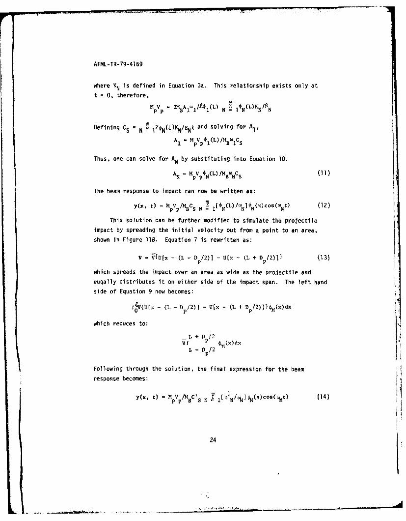
AFML-TR-79-4169
where KN is defined in Equation 3a. This relationship exists only at
t = 0, therefore,
p p Bi1l 1 N I'Nlpp 2 MBAL) I/ () ' 1N L ) N B
Defining Cs = N 1 20N(L)N/aNk and solving for A ,
A I, M pV P l1(L) /MBICS
Thus, one can solve for AN by substituting into Equation 10.
AN = MPVP N(L)/B NCs (11)
The beam response to impact can now be written as:
y(x, t) = MpVp/M 3 Cs N r l[N(L)/WN]IN(X)COS(WN) (12)
This solution can be further modified to simulate the projectile
impact by spreading the initial velocity out from a point to an area,
shown in Figure lB. Equation 7 is rewritten as:
V -V {U[x - (L - Dp/2)1 - U(x - (L + Dp/2)1} (13)
which spreads the impact over an area as wide as the projectile and
euqally distributes it on either side of the impact span. The left hand
side of Equation 9 now becomes:
CV{UT[x - (L - D /2)] - U[x - (L + Dp/2)))H(x)dx
which reduces to:
1 + D /2VI P (x)dx
L - Dp/2P
Following through the solution, the final expression for the beam
response becomes:
p p M BS N 1 lN/ ] O(x)cOs(Nt) (14)
24
AFML-TR-79-4169
where
L + D p/2l - D2 $x)dx (15)
and
C's - N 121NO'N/Nt (16)
Both solutions, for impact at a point and over an area, were programmed
on the computer to be evaluated against test data.
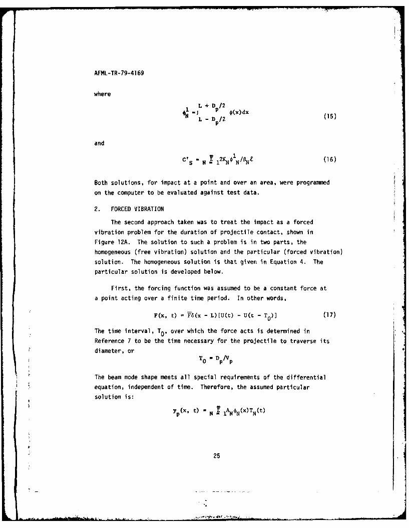
2. FORCED VIBRATION
The second approach taken was to treat the impact as a forced
vibration problem for the duration of projectile contact, shown in
Figure 12A. The solution to such a problem is in two parts, the
homogeneous (free vibration) solution and the particular (forced vibration)
solution. The homogeneous solution is that given in Equation 4. The
particular solution is developed below.
First, the forcing function was assumed to be a constant force at
a point acting over a finite time period. In other words,
F(x, t) = F(x - L)[Ut) - U(t - T0 )] (17)
The time interval, To, over which the force acts is determined in
Reference 7 to be the time necessary for the projectile to traverse its
diameter, orT= D/Vp
The beam mode shape meets all special requirements of the differential
equation, independent of time. Therefore, the assumed particular
solution is:
y1(x, t) N = O(x)TN(t)
25

AFML-TR-79-4169
NMV
Compatibility: MPVP = PBAOf(XTo)dx
F T 6(X-L)[U(t)-U(t-T0))or
F T 63 (x-L) sin (rt/T 0)(U(t)-U(t-T 0)J
y(O,t) o7777 1;z Y. (0,t) =0
A) Forced Vibration At A Point
14VP' p--- Compatibility: M Vp = f.OBAei(x,T )dx
F - {U(x-LeD/2)-U(x-L-D/2)[U(t)-j(t-T0)JOrF- F{U(x-L*D/2)-U(x-L-D/2)}sin(irt/T0)[U(t)-U(t-T0)I
\MM y (0,t) - 0y' (O~t) - 0
B) Forced Vibration Over An Area
Figure 12. schematic of Forced Vibration Models
26

AFML-TR-79-4169
Substituting this into the beam equation, we have
N 1 NON(X)TN(t) - PBAB-IN NNCx)TN(t)
F6 (x - L)[U(t) - U(t - T0)]/EIt
Applying orthogonality, as before, this expression reduces to,
B3MLTM(t) - (PBABt/EI)T%(t) = (FM(L)/EI)[U(t) -
(18)U(t - To )]
For all time except between t = 0 and t = T., the right hand side of
Equation 18 is zero, thus TM(t) is zero for the same time. For
0 < t < T0 , the right hand side of Equation 18 is a constant, therefore,
TM(t) is a constant and the equation reduces to
OMtCM - FOM(L)/Et.
which further reduces to an expression for CM,
CM - FOM(L)/PBAB M (19)
This is the particular solution to the differential equation which, when
combined with the homogeneous solution, leads to the total solution to
the forced vibration problem,
Y t). - N 7 1 ANsin(yc) + BcOCs(N) + CNJON(x) (20)
Evaluating the initial conditions, y(x, 0) w (x, 0) = 0, leads to
YT(X, t) - E 1 lCN[1 - cos(wNt)]4N(x) (21)
This solution is valid for 0 < t < T0, at which time the force is removed
and the problem becomes free vibration with deflection and velocity initial
conditions from the forced response. Evaluating and applying these initial
conditions results in two equations and two unknowns which provides ex-
pressions for AN and B.. The solution for t > TD is then,
27

AFML-TR-79-4169
Yl(X. t) N sin(uN o)sin(Nt) -[1 - cos(wNTo)l
cos(w t) $NY(x) (22)
The only unknown at this point is F, which can be determined from the
conservation of linear momentum assumption. Projectile and beam
momentum are formulated in the same manner as in the initial velocity
analysis, with the additional requirement that the transfer is complete
at time TO. From this, T is determined to be
T= M V Z/CF
where
where F =N l2(L)KNlwN 1tOsi(ANTO)
Hence, CN is
p p N(L)/ B NCS
The forced vibration solution becomes
yT(x, 0) - (M V , F 0(10ON(L)/wN2 MI - cos(W N 0)0N(x)(24)
for 0 < t < T0
and the free vibration solution becomes
1 Xt /M B ~ F 0(4(L)/ 2 ){sin(w T )sin~w 0) -YFxt ( /MBC) N
(25)
[1 - cos(LNTO)]COS(WNt)}ON(X) for t > To
This solution can also be modified, as was the initial velocity
solution, to spread the force over an area as wide as the projectile,
as shown in Figure 12B. The analysis procedure is the same as before
and results in the same solutions as Equations 24 and 25 with two
28

AFML-TR-79-4169
substitutions. 4N(L) is replaced by 1(L) = L + Dp/2 N and CsFiN L - D/2 ON s
replaced by C F N (204(L)KN/N NZ)sinwNT .
A second set of solutions can be obtained by assuming the forcing
function to be a half-sine wave, as opposed to a square wave, acting
over the impact duration. This assumption makes the force take the form,
also shown schematically in Figure 12A,
F(x, t) = F6(x - L)sin(ft/To)0Ut) - U(t - T0)]
and Equation 18 becomes
0ATM(t) - (PBAB /EI)TM(t) [F@(L)/EIt]sin(t/To) (26)
Letting TM(t) = RMsin(irt/To), differentiating, and substituting into
Equation 26 results in the equation
E1 M+ (IT 2 / )M= O(1)I
which, when reduced and solved for RM, yields
RH = F0M(L) /MBCM+ 7T2 IT Oy (27)
This expression is substituted in Equation 20 and solved with initial
conditions for AN and BN to give the total forced response as
yF(x, t) = lRH[sin(irt/To) - (7r/To sN)Sin(Nt)]iN(x) (28)
As before, Equation 28 is used to develop initial conditions at t =T o
for the free vibration solution for t > T0. This solution is
yl(X t) - N = 1 /TOwN) [l + coswN (Y)-
(29)sin(wNTO) cos(UNt) ]N(x)
29
R .1.
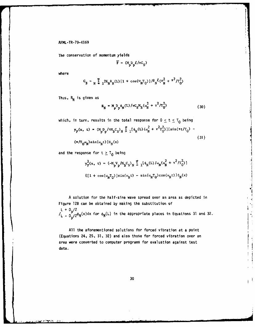
AFML-TR-79-4169
The conservation of momentum yields
= (M DpZ/ Cs)
where
CS=N E % L[ + cos~wNToY1/s t(W N + It /T 0)
Thus, RN is given as
= .P pN (u.s B( +N 02T (30)
which, in turn, results in the total response for 0 < t < T0 being
YF(x, t) = (MpD/MB N 2 + 2T2 )isin(t/TP p N+1 (31)(7r/TowN) sin(yN)] N)
and the response for t > T0 being
YF(x, 0. - (M' P /KBCS)N 1 lN(L)IN(wN + 0~
(1 + cos(wNTO)]sin(Nt) - sin(wNTO)cos(wNt) }4N(x)
A solution for the half-sine wave spread over an area as depicted in
Figure 12B can be obtained by making the substitution ofL +0D/2L- DI2¢N() d for N(L) in the appropriate places in Equations 31 and 32.
All the aforementioned solutions for forced vibration at a point
(Equations 24, 25, 31, 32) and also those for forced vibration over an
area were converted to computer programs for evaluation against test
data.
30

AFML-TR-79-4169
SECTION IV
NUMERICAL ANALYSIS AND RESULTS
Each theoretical solution derived was programed for analysis on
the digital computer. The program was written for use at an interactive
graphics terminal so that several parameters in any particular problem
could be easily varied and results compared. The required input included
beam parameters (dimensions, material properties), projectile parameters
(diameter, density, velocity), the number of modes to be used in the
summation, and the time period over which to make strain calculations.
Damping effects could be included, at the user's option. When included,
damping was modeled by decaying exponential functions applied to each
mode. The values of included in the program were based on actual
damping measurements taken from each test specimen.
Initially, numerical difficulty was encountered evaluating sinh and
cosh functions for large values of . The problem arose in calculating
K in Equation 3a and stemed from taking small differences of large
numbers. As R increased, so did the values of sinh and cosh until the
accuracy of the computer was exceeded. The problem was solved by
expressing hyperbolic functions in the mode shape equation as exponentials.
A complete derivation of the expressions used to calculate O(x) is included
in Appendix D. Once the exponential equations were included, all numerical
problems were corrected and accurate solutions were obtained from the
program, which are listed in Appendix E.
Results calculated and included in the output were the maximum
absolute value of strain calculated over the specified time period, the
time at which it occurred, the resonant frequency of each mode used in
the summation, and, if desired, a plot of strain versus time. Figure 13
is an example of the program input and output and Figure 14 exemplifies
the type of strain/time plot generated. The program was used to calculate
theoretical impact responses for comparison with each other and with
experimental results.
31

AFML-TR-79-41 69
Win t)'ommmmmv4 Q LL 0 0 c.C> o
c. 7'++ + ~+th CD0 0 kW l. LU L
9 * U) Q). -3 -4 -4-4 .- 4-% LI L-J r v tr tr vr
0 n (n) 0 MMCic
I-L => -J~~ *S %* I
L I .. C%, C . f. .) co O dS + I- I
I-CL
oz rU-C 0CZ 'CU) U U) 41
JO CL C~W C>L& th C- 0 1
0 - - I. - I-.J Ch f-7 7:o N.
U s4C W w+I
I I-~c O- LC. e > -3J) i W-OC" -4(1Wr
U= -0 C41 I- C) :- W.LL r- M 0z . a O.C)( -4 ") - 4; . * **
0 -%4~ r- wo cu Inc3I-L W-i C ,4) 4-:e4
610D~o "-oOtjici row. ejLUL C ~ (X%- &Z>- C-) (a
:> W w 1- 4 .I
o J I o " S -
0 1C k C C L-% 4 -- t i .
W -> -40d .L.Af- W IL)1 ;-) )C
1 -0 - - j--< o ~ 0)t cU)Io~ ~ nn u o (uQ& I-
E ~ ~ C OQ0.Ii~J M .
=w w Q- -- tj0 a

AFML-TR-79-4169
__ 0
nIn
'-
s,,.
C V--
U,
0 -i
CD~
33
.... - - i mr.. . . .. . .. . .
i ! . :'= ... ,, - " ":._,,.
.,, .. ... ..... - . . ,
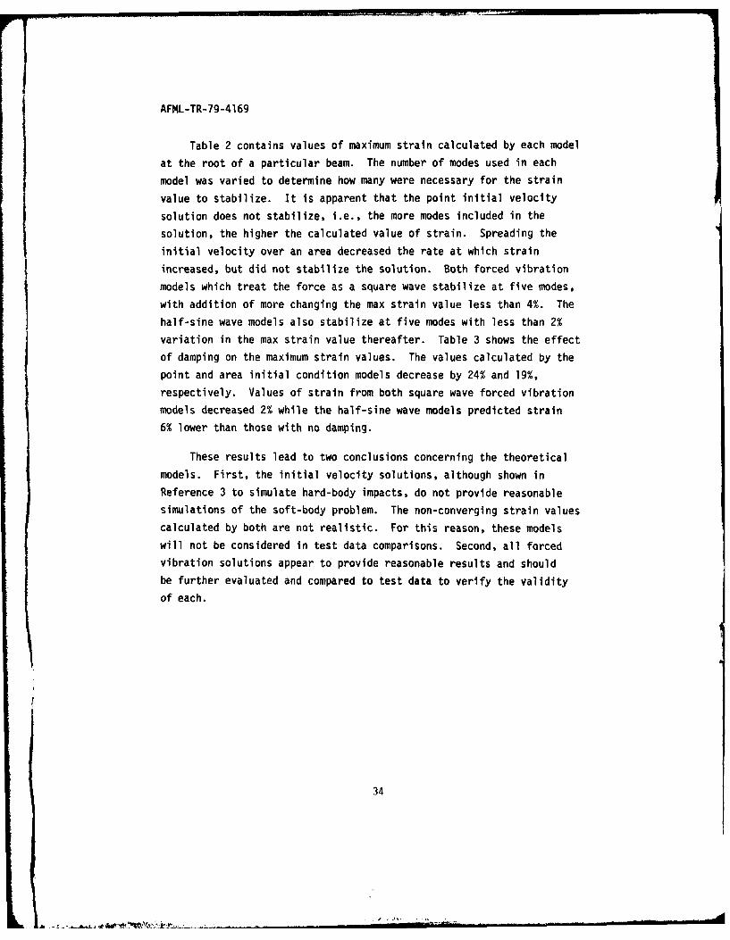
IAFML-TR-79-4169
Table 2 contains values of maximum strain calculated by each model
at the root of a particular beam. The number of modes used in each
model was varied to determine how many were necessary for the strain
value to stabilize. It is apparent that the point initial velocity
solution does not stabilize, i.e., the more modes included in the
solution, the higher the calculated value of strain. Spreading the
initial velocity over an area decreased the rate at which strain
increased, but did not stabilize the solution. Both forced vibration
models which treat the force as a square wave stabilize at five modes,
with addition of more changing the max strain value less than 4%. The
half-sine wave models also stabilize at five modes with less than 2%
variation in the max strain value thereafter. Table 3 shows the effect
of damping on the maximum strain values. The values calculated by the
point and area initial condition models decrease by 24% and 19%,
respectively. Values of strain from both square wave forced vibration
models decreased 2% while the half-sine wave models predicted strain
6% lower than those with no damping.
These results lead to two conclusions concerning the theoretical
models. First, the initial velocity solutions, although shown in
Reference 3 to simulate hard-body impacts, do not provide reasonable
simulations of the soft-body problem. The non-converging strain values
calculated by both are not realistic. For this reason, these models
will not be considered in test data comparisons. Second, all forced
vibration solutions appear to provide reasonable results and should
be further evaluated and compared to test data to verify the validity
of each.
34

AFML-TR-79-4169
TABLE 2
THEORETICAL RESULTS WITHOUT DAMPING*
5.6 INCH BEAM; Pp = 0.032 ibm/in; Dp 0.5; Vp = 340 f/s
Number f Croot,%of K------r- -
Modes I PIC AIC F FA FV' FA'
II ,1 0186 0.1 0.187 0.187 0.187 0.187
2 0.149 0.091 0.150 0.150 0.201 0.201
30.328 0.182 0.267 -0.264 0.266 0.264
4 0.400 0.214 0.329 0.323 0.287 0.2S4
0.458 0.241 0.327 0.321 0.292 0.289
* I10 0.578 0.285 0.339 0.330 0.288 0.284
'20 0.990 0.348 0.340 0.332 0.287 0.284
PIC = Initial Velocity at a Point
AIC = Initial Velocity Over an AreaFV - Forced Vibration at a Point; Step-Function ModelFA - Forced Vibration Over an Area; Step-Function ModelFV' - Forced Vibration at a Point; Half-Sine Wave Model
FA' - Forced Vibration Over an Area; Half-Sine Wave Model
* Strains are absolute value
35
. l .i , : ~~~~i- . .. . . . . . . .. " '''""-.. .. . . ". .". . . ... . .

AFML-TR-79-41 69
TABLE 3
THEORETICAL RESULTS WITH DAM4PING*
5.6 INCH BEAM; pp = 0.032 ibm/in ;p = 0.5; VP 340 f/s
ofube £root'% -
of: ---- AIC F - - - - -Moe PF AC IV FA FV' FA
[ 10 0.4381 0.230 031 0.323 0.270 0.267
*Strains are absolute value
36
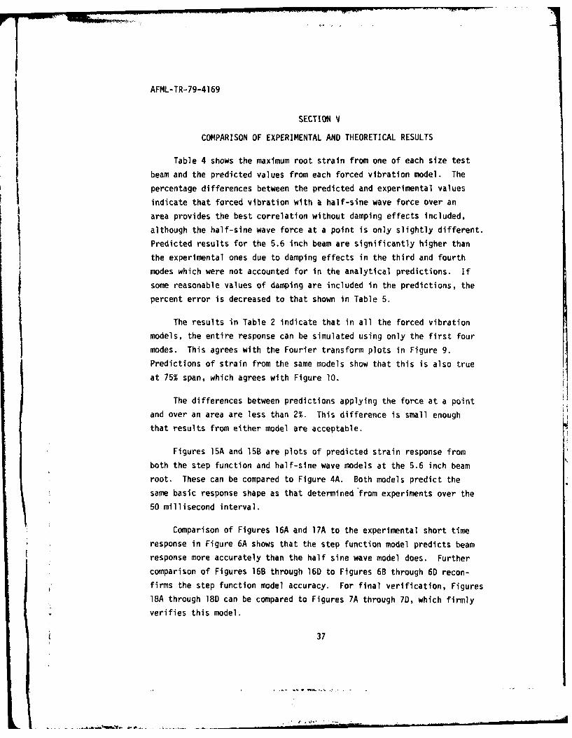
AFML-TR-79-4169
SECTION V
COMPARISON OF EXPERIMENTAL AND THEORETICAL RESULTS
Table 4 shows the maximum root strain from one of each size test
beam and the predicted values from each forced vibration model. The
percentage differences between the predicted and experimental valuesindicate that forced vibration with a half-sine wave force over an
area provides the best correlation without damping effects included,
although the half-sine wave force at a point is only slightly different.
Predicted results for the 5.6 inch beam are significantly higher than
the experimental ones due to damping effects in the third and fourth
modes which were not accounted for in the analytical predictions. If
some reasonable values of damping are included in the predictions, the
percent error is decreased to that shown in Table 5.
The results in Table 2 indicate that in all the forced vibration
models, the entire response can be simulated using only the first fourmodes. This agrees with the Fourier transform plots in Figure 9.Predictions of strain from the same models show that this is also true
at 75% span, which agrees with Figure 10.
The differences between predictions applying the force at a point
and over an area are less than 2%. This difference is small enough
that results from either model are acceptable.
Figures 15A and 15B are plots of predicted strain response from
both the step function and half-sine wave models at the 5.6 inch beam
root. These can be compared to Figure 4A. Both models predict the
same basic response shape as that determined from experiments over the
50 millisecond interval.
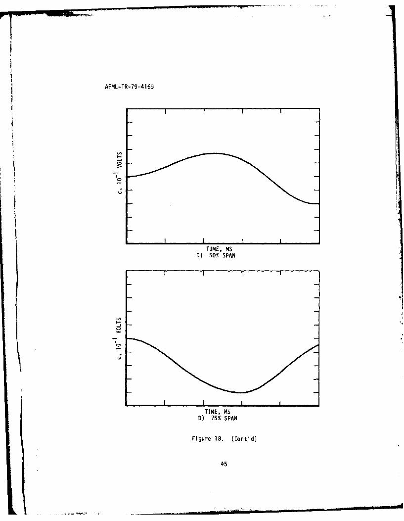
Comparison of Figures 16A and 17A to the experimental short time
response in Figure 6A shows that the step function model predicts beam
response more accurately than the half sine wave model does. Further
comparison of Figures 16B through 16D to Figures 6B through 6D recon-
firms the step function model accuracy. For final verification, Figures
18A through 18D can be compared to Figures 7A through 70, which firmly
verifies this model.
37
AFML-TR-79-4169
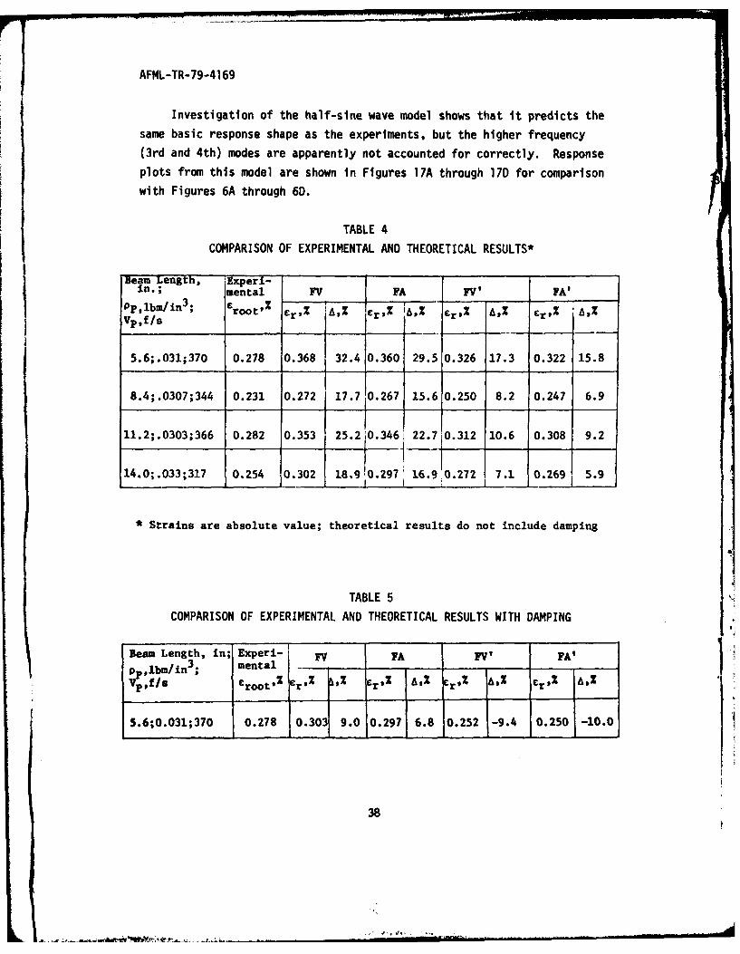
Investigation of the half-sine wave model shows that it predicts the
same basic response shape as the experiments, but the higher frequency
(3rd and 4th) modes are apparently not accounted for correctly. Response
plots from this model are shown in Figures 17A through 17D for comparison
with Figures 6A through 6D.
TABLE 4
COMPARISON OF EXPERIMENTAL AND THEORETICAL RESULTS*
Beam Length, ;Experi- Iin.; mwental FV, FA F FA'0P, zbm/in3 ; root'% crozj, ErI&A cr,Z AArZi,,Vp,f/sI
5.6;.031;370 0.278 0.368 32.4 0.360 29.5 0.326 17.3 0.322 15.8
8.4;.0307;344 0.231 0.272 17.7,0.267 15.610.250 8.2 0.247 6.9
11.2;.0303;366 0.282 0.353 25.2 0.346! 22.7 0.312 10.6 0.308 9.2
14.0;.033;317 0.254 0.302 18.910.297 16.9.0.272 7.1 0.269 5.9_I _
* Strains are absolute value; theoretical. results do not include damping
TABLE 5
COMPARISON OF EXPERIMENTAL AND THEORETICAL RESULTS WITH DAMPING
Beam Length, in; Experi-' FV IA FV' PA'~~1 i 3; mental F A
Vp,fls CrootZ F, cr1Z as% r,% A, r,1% ,
5.6;0.031;370 0.278 0.303i 9.0 0.297 6.8 0.252 -9.4 0.250 -10.0
38

AFML-TR-79-41 69
0 020 3040 50
01
TIME, MS
Vba)io Ste-uclosoe
39 I3A

AFML-TR-79-41 69
TIE MS
04

AFML-TR-79-41 69
TIME, MSC) 50% Span
411

AFML-TR-79-41 69
CD,
TIME, MSA) Root Locatin
Fiue1. Sri i 40Ic emFrmHl-ieWv
Moe-(. m.
04

AFML-TR-79-4 169
CDI
C,)
TIME, MSC) 50% Span
TIE MS
0)75 Sa
Fiue1. Cnd
04

AFML-TR-79-41 69
TIME, MS
A) Root Location
.)-j
TIME, MSB) 25% Span
Figure 18. Strain in 14.0 Inch Beam From Step FunctionModel (0.5 ins.)
44
AFML-TR-79-4169
CDI
TIEM
C)50 SA
TIME, MSC) 5% SPAN
Fiur 18 Iot
-45

AFML-TR-79-4169
SECTION VI
DISCUSSION AND CONCLUSION
The experimental data provided an excellent base from which to
evaluate theoretical models. Both the FFT system and the high speed
transient recorder proved to be very valuable tools for studying the
impact problem. Fourier transforms of test data made it immediately
apparent that the initial velocity solutions were not adequate models.Also, the very short-time response plots from the transient recorder
dispelled any questions of high frequency bending waves causing
responses the FFT system could not record.
Both the strain values and graphic displays of beam response data
allowed complete verification of the step function forced vibration
model. Correlation between actual data plots and the predicted
response was surprising and proved to be the discerning factor
between the step function and half-sine wave formulations. The only
question that might arise would be why the half-sine wave model more
closely predicts maximum strain. The answer to this may be in the damp-
ing present in the beam/fixture system. Accurate modal damping values
could not be obtained while the beams were mounted on the impact range;
thus, any values employed in the models were approximate. Conceivably,
if the actual values for each mode could be modeled into the computer
simulation, values of strain predicted would be much closer to experi-
mental values. Additional damping could also enter the system through
the projectile/beam interface. Plastic flow and many other undefined
phenomena taking place in the projectile during impact could causesmall reductions in beam response.
The beams tested were specifically chosen to approximate the
stiffness of typical jet engine fan blades. Timoshenko effects were
negligible in this base because high order modes did not lend any
significant contributions to beam response. For beams of different
geometric properties where A/t (modal wave length/beam thickness) reaches
ten in the first several modes, the impact problem requires Timoshenko
beam theory to account for shear and rotary inertia. However, as long
46
AFML-TR-79-4169
as X/t is greater than ten, an Euler-Bernoulli beam theory formulation,
which models soft-body impact as a forced vibration, treats the impact
as a step function force in time and assumes a complete momentum transfer
from projectile to beam will provide a good solution for elastic beam
response. The accuracy of results from such a model is good for short-
time response and can be improved for long-time response by addition of
damping effects. Future work in this area can build upon this basis and
the fact that linearly scaled beams and projectiles will produce equal
strains. This means that the response of very large beam-like structures
to soft-body impacts can be determined from analysis or testing of
scaled-down models and the results will not require scaling.
47

AFML-TR-79-4169
APPENDIX A - ESTIMATION OF PROJECTILE VELOCITY
According to Reference 6, the stress at the beam root is
aoot KAXh/2I0
where
X E Impact Location
h B Beam Thickness
10 = Minimum Area Moment of Inertia
The values of X, h, and 10 are determined directly from the particular
beam geometry. K is the equivalent beam stiffness determined from
Figure 5, Reference 6 as a function of impact site. A is the effective
first mode amplitude at the impact site. For a strain of 0.25%, root
is 25,000 psi which gives A as
A = (50,O00)10 /XMh
For the 8.4 inch beam,
A = (50,000) (0.0017086)/(6.3) (202) (.225) = 0.299 in.
Assuming simusoidal motion,V = Aw
where w is the effective first mode frequency, determined from
W - KH
M is obtained from Figure 6, Reference 6. Thus, we have
w - 202 x 386/.227 - 586 HZ
Thus, the velocity isV - Aw - 175 in/s
Assuming complete momentum transfer from the projectile to the beam,
the projectile velocity can be approximated by
VPWVBM/M
Vp - p
V 4
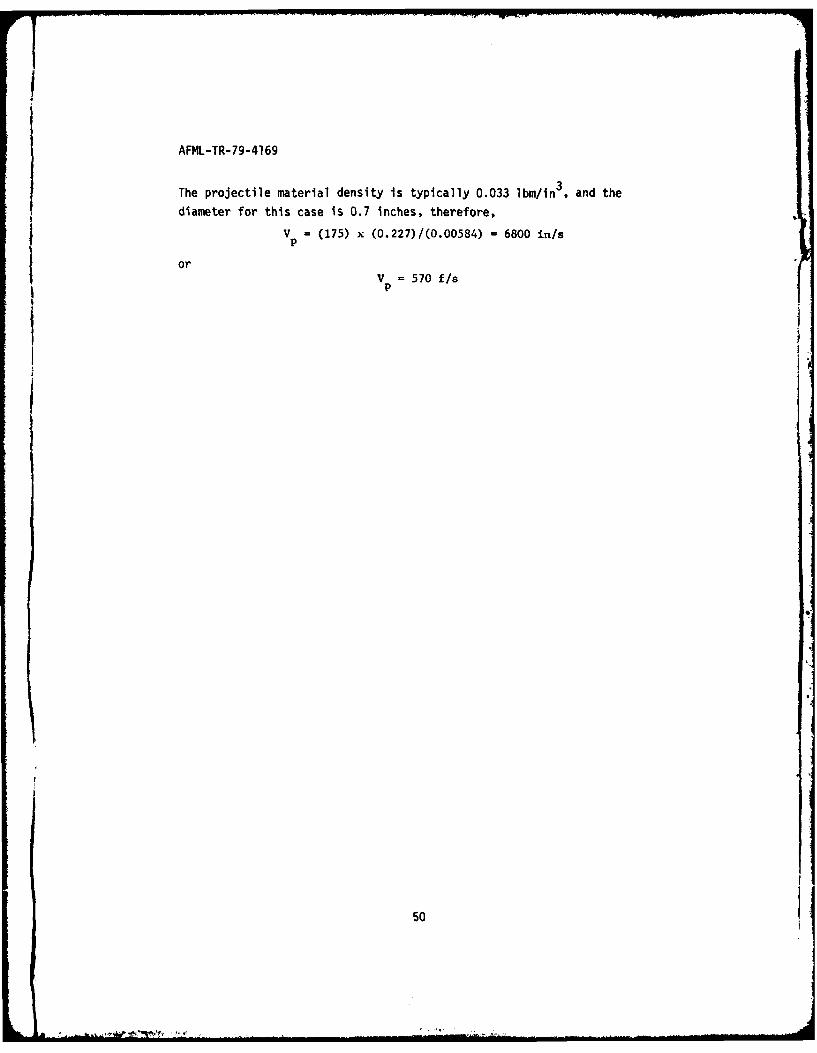
AFML-TR-79-41 69
The projectile material density Is typically 0.033 ibm/in, and thediameter for this case is 0.7 inches, therefore,
V = (175) x (0.227)/C0.00584) =6800 in/s
or V = 570 f/s
50

AFML-TR-79-4169
APPENDIX B - STRAIN IN LINEARLY SCALED BEAMS
The elementary formula for bending strain in a beam is:
E = Mc/IE M Bending Moment
c = Distance from NeutralBending Axis
I E Moment of Inertia ofBeam Cross-Section
Er Young's Modulus
For two linearly scaled beams,
, =wt3/12 12 = (K)w(K3)t 3/12 =K411
andc2 f Kc1
Therefore,C 1 =f Ml1ClI/Il
and 2 M2KcI/K 4I1 E = (1/K3)M2c/1 1E
The bending moment, M, is created by a force that is proportional to the
momentum of the projectile.
1 0Fdt m V F mmV/T m Projectile Mass0 p p p P P
V = Projectile VelocityP
T 0 Duration of Impact
51
AFML-TR-79-4169
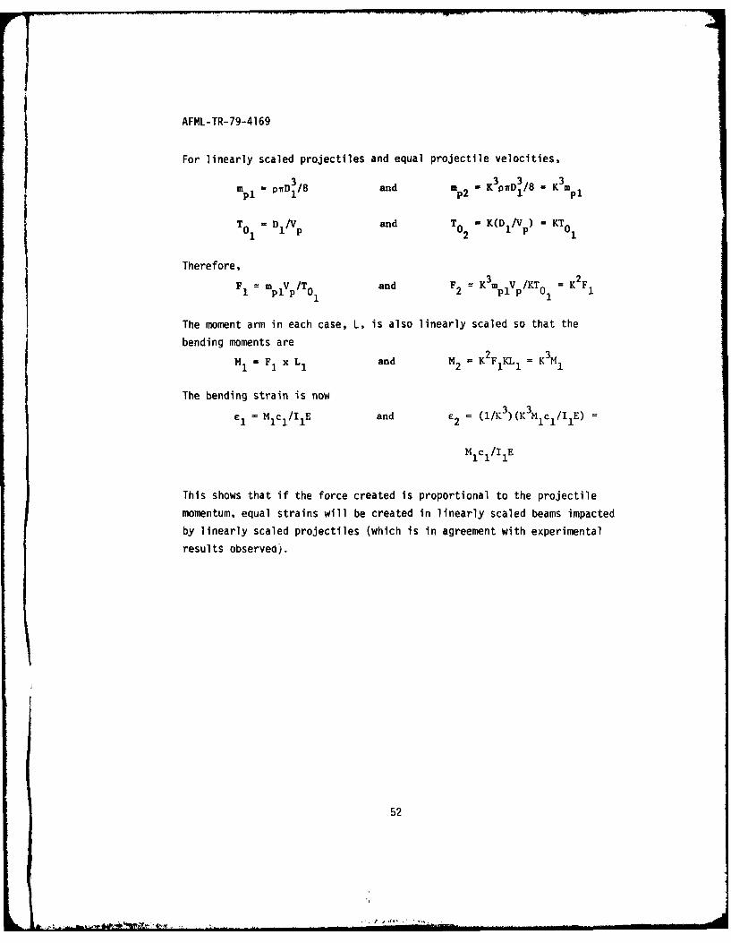
For linearly scaled projectiles and equal projectile velocities,
p =i DA/8 and ap2 K3 prD3/8 - K3m
TO D /V and T0 = K(DI/Vp ) = KT0
0 1 P0 2 1 01
Therefore,
F1 P pVp/T01 and F2 = K3mplVp/KT0 1 = K 2 F1
The moment arm in each case, L, is also linearly scaled so that the
bending moments are
M 1 F1 x L1 and M2 = K2FIKL 1 = K3 l
The bending strain is now
1 = MICI/IIE and £2 = (1/K3)(K3M1C1 /11E) =
MIC1 /I 1E
This shows that if the force created is proportional to the projectile
momentum, equal strains will be created in linearly scaled beams impacted
by linearly scaled projectiles (which is in agreement with experimental
results observea).
52

AFML-TR-79-4169
APPENDIX C - EVALUATION OF TIMOSHENKO BEAM THEORY EFFECTS
When modes of vibration are considered in an analysis, the Euler-
Bernoulli Beam Theory provides adequate eigenvalue predictions up to
a certain point. When the effective wavelength of a particular mode
is of the order of ten times the thickness of the beam being considered,
shear effects start to become significant and the Timoshenko Theory is
necessary to make adequate elgenvalue calculations. Figure C-1 is a plot
of effective wavelength to thickness ratio versus mode number for a
cantilever beam. This indicates that for the beams used in the impact
experiments, shear effects will be negligible until the twentieth mode
of the smallest beam. The lowest curve on Figure 16 represents a beam
of thickness equal to one-fourth its length. Analysis of this class of
geometries should employ the Timoshenko Theory to predict impact response
accurately. Since only the first four or five modes were apparent in
test data and the same number were necessary in theoretical predictions,
the Euler-Bernoulli Theory is adequate to model the soft-body impact
probiem as considered in this analysis.
53

AFML-TR-79-4169
10 1000.-T
765
I'
/ 0 14g.0 IN. TEST BEAM
05.6 IN. TEST BEAM
1 100. 5.6 IN. BEAM; t/2. 0.25
6 O5
2
110.0
765I.
3
2
1 1.0
1 0.11 5 10 15 20
NIE NUNS)ER
Figure C-1. Shear Effects in Cantilever Beam Vibration
54

F m~v ..... "1 -4,-..... .
AFML-TR-79-4169
APPENDIX D - NUMERICAL STABILITY
#N(x) - cosh( NX) - cos(N x) - f[sinh(Ot) - sin(O 1t)]/II[cosh(Bot) + cos(BNL)1](sinh(.,,x) - sin(8x) ]
To evaluate this expression on a computer, the hyperbolic functions
must be expressed as exponentials. This leads to
#,(x) - (1/2)e X(l - N) + (l1/2)e-NX(1 + KN) - cos( 8~x) +
KYslN(8x)
where
[e1 - e-Nt/2 - sin(0Nt)/[eVlt + e-13it/2) + cos(Nt)]
For %Z = 17.2787595323 (mode 6), KN = 1.000000063. For a 16 bit word,
the computer carries seven significant figures, and thus, would make
1 - K6 Identically zero. eN for mode 6 is on the order of 3 x 10⁷ so
that (1 - K6)e86Z would have a significant contribution to sine and
cosine functions. Double precision will not change with phenomena for
higher modes, so a convergent solution must be sought. First, in the
expression for KN , let cos(ONI) = - ]/cosh(ON' ) and use the identities
relating cosh and sinh to obtain
%- 1 - (2e"BNtsin(BSt)/1 - e- 2 1N ] [ 1 + e- 2BN)( - e20N) ]
Substituting the series expansion
1/1- U - + U +0 2 + + .
and letting
t' 2(e- 2 t + e- 0 t + e +60Nt .
55
z.
AFML-TR-79-4169
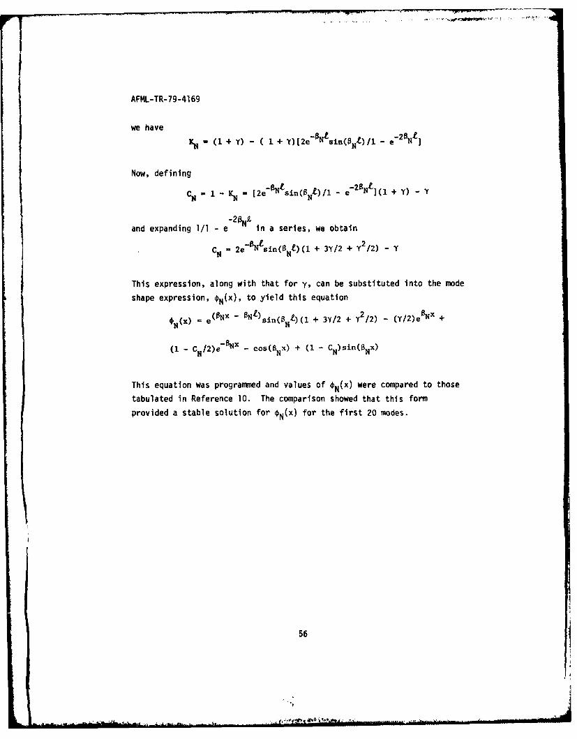
we have we (1 + Y) - (I1 + Y)[2e- Ntsin(N-)/1 e-28Nt ]
Now, defining
CN1 -1 = [2e-BNtsin(PNZ)/1 - e-28N]( 1 + Y) - Y
and expanding 1/1 - e in a series, we obtain
2CS . 2eONsin(N t)(1 + 3Y/2 + Y /2) - Y
This expression, along with that for y, can be substituted into the mode
shape expression, ON(x), to yield this equation
iN(x) - e(ONx - Nt)sin(SN t)(1 + 3Y/2 + Y2/2) - (Y/2)eBNx +
(1 - CNI2)e-ON x - cos(%ex) + (1 - CN)sin
This equation was programmed and values of ON(x) were compared to those
tabulated in Reference 10. The comparison showed that this form
provided a stable solution for *N(x) for the first 20 modes.
56

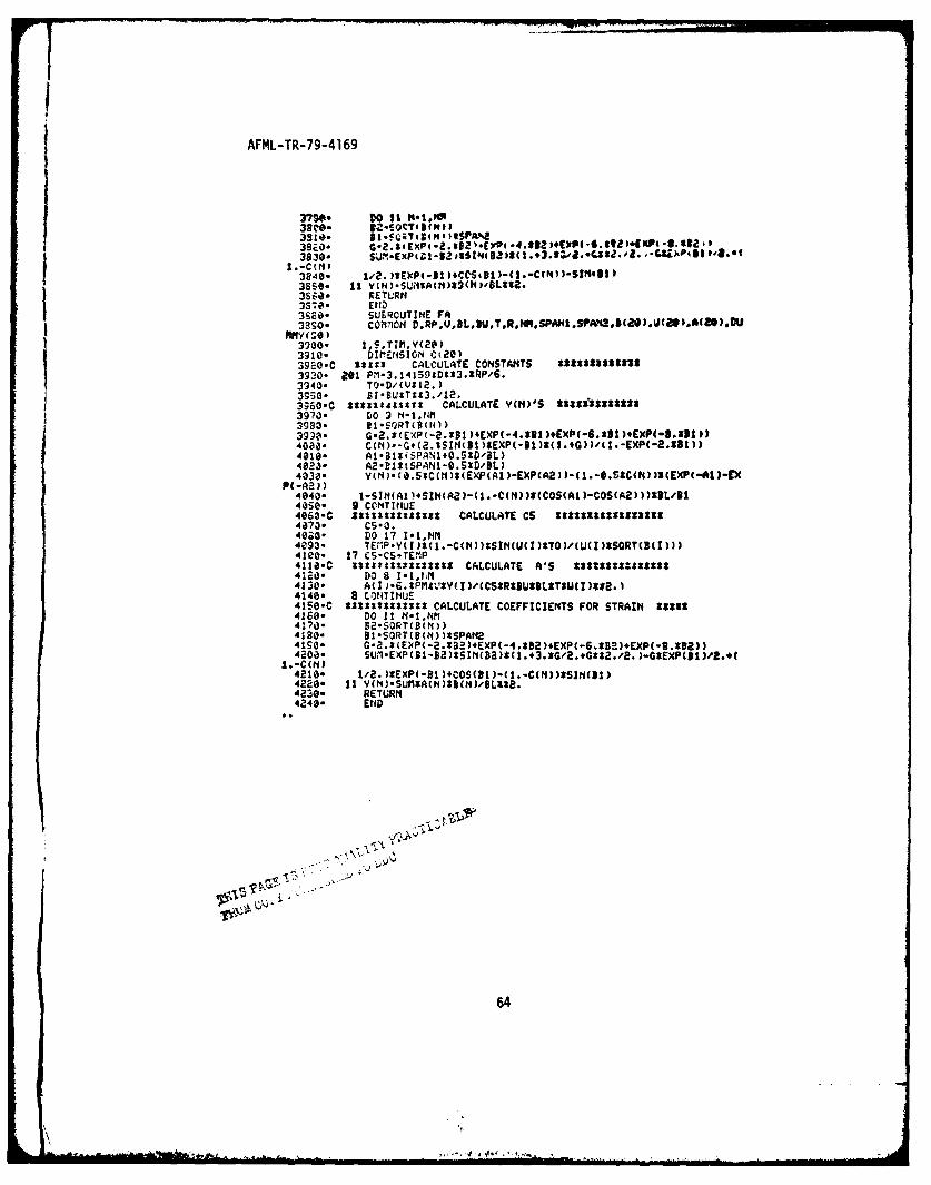
AFML-TR-79-4169J APPENDIX E -LISTING OF COMPUTER PROGRAM
100- OUERLAYEZMPACT S*O1110- PRO~cPA.'1 tPd'uOUJ?120. CC'tlON D~~,Ls.~...PlS~.(g.~8IA*
130-c 1,S.TIMnYv;O,.PS1 W-0,7T.fln SIC.O OEDu .t40-C IS$ THIS PROGRNM CA~LCULATES THE SWRAIN It$ A CAWIRLELIE HEAP
at4 )10.99SS4074912.210- f(1417C~9S2220' ()1.7SS52z2
240. PB)-23.5614493112.250 (.o7235S2263.a-8S1Z12273. S1j .36 z122
B(14)42.41551112.
.1. (15)*4 SS30934702.
340- B1S4.9'?371431s2.:?So-g.5.1~44~:2
3e' B23 ) 61. 261056749:22.37-3 J.320. PRINT 152.30IS2 FORtiAT(XflODEL OPTIONS ARE-*,/.1oIXPON7 I.C.-NITIAL VE
LOCITY400- 1AT A POINT 'I. AREA I.C.-INITIAL VELOCITY OVER AN AR
EA410- 1,/10X. rCP.CED VIBRATION AT A POINT 4,/1GX,'FORCED IBRAT
IO1N OVE420. IR W~4 AREA ',/IOEND')43-0. 178 PPI14T 153440.10 FCRNATX,*OPTION-1)450. FEAD 2S4,AD463- 2S4 FORMAT(A2)473. IV'.A!.EO.HE)GO TO 1764E8%-154 FQOI1ATCA1)4 '3. PRIIITZ, *CO YOU UANT DAflPIN?-9
S0- REA~D 154,ADSI0. 1F(AA.EO.zHv)GO To Z01520- 203 PRIN!:. HOU MANY MODES DO YOU UAM? TO USE 9 -
540- IFC~b'M.EO.1HY)G0 TO 202550. 199 PRINTW.ENTER THE DIMENtSIONS, DENSITY& AND MODULUS Of YOUR
BEAM.,560- ZS PR1NTt,'LU..RO.AND E570. REA2.0L,PUTR,E580. IF(AL.EG.IHY)CO TO C02S90- 205 FRII4T:.'ETER IM'PACT POINT AND POINT FO*CSTRAIN CALCS IN
OF L-See. to
tills ?IAGE IS BE-3T ~AA'~ __TO 10
57

AFML-TR-79-4169
64- If - L.E2. Ik,' )^QC 2041650.20 P:4Tx.c11TER DtAK'PEM. DENSI~. 0^9 4LOCZTV OF t(P*CJEC
TILE0 1.
60 IFoAhK.E0.1HVlGO TO tlm1690-206 FRINT2.1UHAT TIME PERIOD DO YOU WANT TO CALCULATE St"aI" OUD
700. 1. SO, S, OR 0.5 MS.)710: PE-411.IMa0TE~L:
T CIMTIM1.000'-~ IF(AB.EQ.HIG TCAL 1C
750-C 2221tIt*~S CALCULATE T RAlhIE zSa~ss:*~~760 20 C '(V6112.)SR(.*)B~t.
77- DO 61 -1.10HM
9.2e. Z*0.-()C730' C0 3 .TWU I950. 20 IFJA.E.2OR.J.g.33zePIC~870. IF(AB.EG.2HAIZ.0. AI83 IF(A9.EO.ZF'fCLc TO 7933' IF(AB.E0.2HFA)COL TOA7
U(J -TID,(II
90- 13 EPSI.EScs
2. IT-I.1110' 12 12 1-1,10UE
11ao- Tf9-TI+.TIM.110 PRNT30ST
920
93- 3JIu90. .. AJ9tAfDL.Eg.Z9.*95- I(.G2O..03Z0r9
960- FQ.^.4)Z-.0 58

AFML-TR-79-4 169
1160- 390 rORfAT(2X(,*THE fx MaiJn 19 I.ESf.6. OCCVtmG Of 11 6I
1190- PRINT$, ImotE FRfGU(4v. Nz. cocrric:tt#? V:A.
i120. IVEL, FI'
I024,k) Al .NtN
12%- PR:NT 1OI1t4,UVAI.D.V
I Eso' 10 CO;NT114LE12~0- 30 FRIiTl,'PLOT?£37- FEAD 154.AIJK£230- IF'AlJ\.E.HYlGC0 TO 31
12%. GO TO 29
131,0- 29 PRIN71*LIOJLD YOU LIKE THE SAME PROBLEM, DIFFERENT 0PTIOn'p
1320, REemD 154,AA£338. IF(A.EQ.1HY)GO TO 17813413 PRIriTS,. -JCULD YOU LIKE TO CHAMIE THE NUMBER OF MODES?
CT ?0 :RIT9'UiL YU LIET CHANGE THE TIME PERIOV'
10- IFAKKE.l4Y1GO TO 20514,30- 2 PRIrif. AJULC YOU LIKE THE SAMlE PRBEM ITH DIFFERENT IPROJ
141.0. 17P1- OCTOS1430. RE.;D 1S4.ALL142-3 IF(AL'8E.HY)GO TO 20514S0- 23 PRINTs. UOULD YOU LIKE AH SAMFERETAM WITH TH DI MEN PROJE
CTILE-'14 ' (O. 1"-.
14k. READ 154.'AL14-0- IF(AK.E-O.1NY)GO TO 1094S~O. 24 FRINT5,*UOULD YOU LIKE A DIFFERENT BEAM AITH THFESAET PROJE
CT1LE
1563- READ 154,AL15!k- IF(A.E0.IHY)CO TO 199
56- GO TO t7S1570-176 CONTINUE
ls~- ENDIS90- SUBROUTINE PLOT(X)
16-- COMMfON D,RP,U.BL,BU.T.Nt.SPAN1SPANBCL4 ( ),A(26).DU
1610. 1 S.TIMY(20).EPSc1,es).TTIM1620- DIMENSION X(1000).ITCS,1630. CALL INITTCI20)1640- IF(A8S(S.LT.0.00142IS)YMn.
59

AFML-TR-79-41 69
17- CALL Cd3O.~4-~~~1623- CALL ~JD~3,2.S,63
CA20 iifE-.0U0~1.(176. CALL tRAUA(0 .)
173 CALL rRAUAJT0.X-v)1748 10 pTITl+'5. M
17CL4. CALL MCOUEA(1tR,-VM)1S4F,. CALL DRUA(Tr,-'Y+ms.4
07- CALL t .RA TI MVM)18EO. 11CALL DPRAUAWI.YM-YU.1970' CmLL TSEND1830- R-TM/S
190 DO 1 1.1.4
1250. CALL fl)'EA ( S. Y )i1860E 11 CALL DPALJA( TIS,RY*)
17- CALL CHRSZ'4
1830. CAP O&AS(,2GIso O12TIEO~ G TO 100
23900 RF(1.EO.2)t.41
210. 12 CALL Q.UACBI-.2ST4 P195e COL T EI0D
122 CAL IF(I.EO.4)LL2H20"o0. CALL( QES(J9L.44020:4). IFCI.EOj.!)LBL.2HO.216"'0. IO TME-0G 11010323Eilb-00 IVCIE0.2)LBL-2.12390. I(I.E0.3)LL-2H2
2.7- IF(1.EO.4)LBL-2H.3
21:3- 00 IFC.EO.2L9L2I
21so* IF(I.E0.6)LBL-2H50
21e 100 11% 2EQ.C22AL-rHI
60
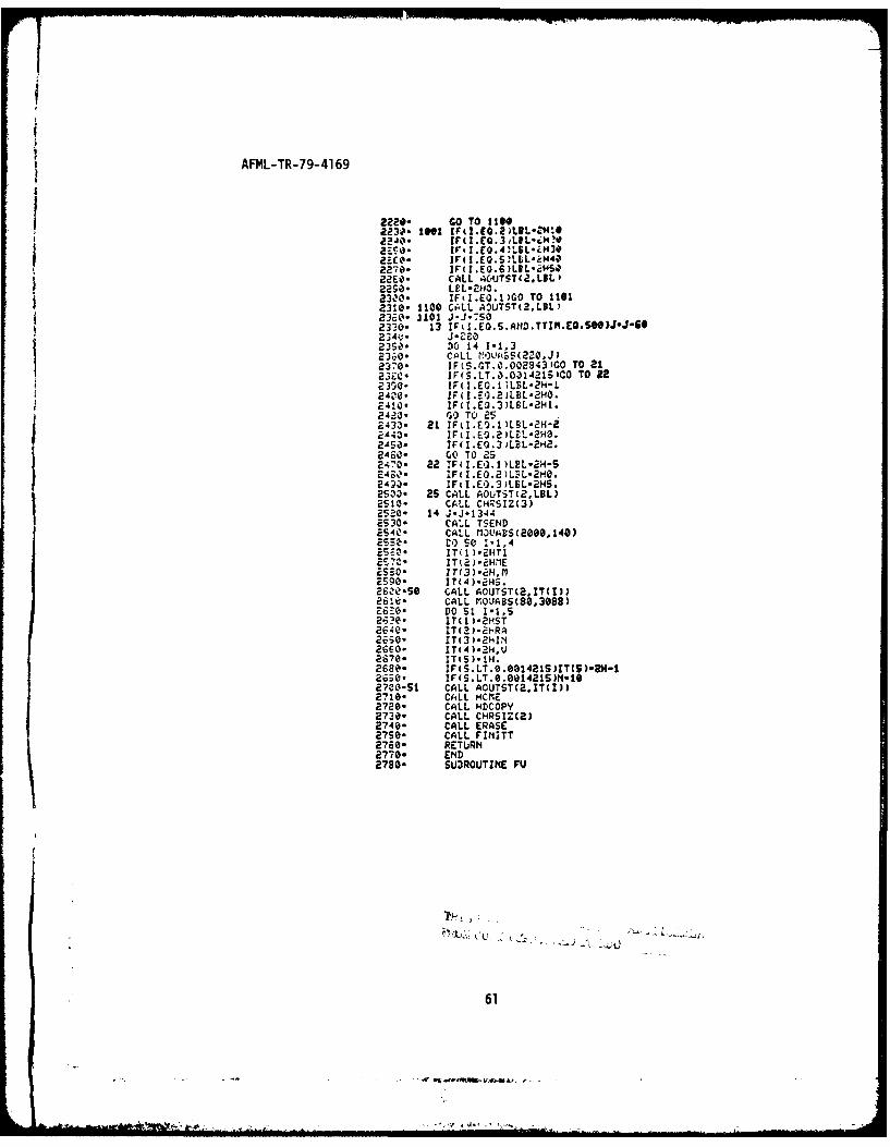
AFML-TR-79-4169
2220- go TO I M
2230- C L C'01(.LL22580-
2310*110 CA~LL ACOUTST(2,LBLI
2320- 1101 J.J.50o2330- 13 IFtl.EO.S.ANiD.TTZN.EO.S*)JJ-6234?~- Za2350-.4 DO 14 1-1,3
2N. CALL N-WtAS(220,J)23 ;1 0. JF(S.6T.O.002343 'CO TO 2123 -0. IF(S.LT.O.0314215'CO TO 22
r'iEO1)BL2-40- IF(I.EOQ.2jL8L.2H0.
F4:0- IF(I.EQ.3)LBL-2Hl.CO;3 TO 25
c433- 21 IF(I.EQl.11LRL-2H-ZI244-;3 IFiI.E0.2ILEL-2HO.2ASO. IF(I.EG.3iLBL-2H2.2460- GO TO aS) 247'0- 22 I(
249.)- lFtI.EG.3)1LEL245.2533- 2S CALL AOUTSTt2,LBL)2510. CALL CH;ZSIZ(3)2520- 14 J.J.13442530- CALL TSEND2540- CALL MOVARS(2000,140)
FSFZ So 1.1,42520. ITtl).2HTI
e550- ZT(3).EHIM2S90. IT(4).2HS.UZ40-SO CALL AOUTSTC2,ITC!))
2e. CALL rOVJABS(80,3088)ZG620. DO 51 1-1,S2-;;0- IT(1I.2HST
2e. IT()2R2650- IT(3).2H1I.*2660- IT(4).2HV2670- ITtS)-'H.2680- IF(S.LT.9.001421Sfl715).2M-l2630- IF(S.LT.G.001421S)N-10273.0-S1 CALL AOUTST(2.IT(!3)2718. CALL HCMEZ2720- CALL H.DCOPY273a. CALL CHRSIZ(2)2740- CALL ERASEZ750- CALL FINITT2760- RETURN2770- END27801- SU3ROUTINE FU
61

AFIL-TR-79-4169
2?90. COMMUOh
asuo. 1.S.Ti!Y(021. DlrErNSfoN Ciao
ZS20-C W352 CALCULATE CONSTANTS2330- 201 FM.3.14159$DSt3.SQPe6.2940. TO-D/cUS12. )
2SCO-C S*33*3tis: CA~LCULATE V(N)5 333338313 S33S8230- D 9 H-.NazI.l 91Q5RT ( S(N2,)- G.2.S(EXP(-.K31lEXP(-4.S)EXP(6.331)CXC-(8.'SI
29e (N)-E\P(fRG-D1)SSIN(3I)3(1..3.)G/2.4C23Z./2a.-G*EXP(ARG)'ZL
E340. 9 CONTINJE2950-C zstt s34 CALCULATE CS 3332*Z
,04,)- CNTM~UEug**11a81828 CALCULATE COEFFICIENTS FOR STRAIN 23233333
DO it tt'1.NtIt2.soprTC(N))
30-3 I. SRTtS (N I ISPAN213- G.2.ILEiP(-2.232)4EXcPC-4.:32),EXP(-6.3521,CXP(-g.2B21)
3Ik- 112 ~ u*xc3-1)CSz(I )(1.,32a.CN)*Ss2,8I-*x(u1/2
3120- 11 Y(N)-SUM*A(NI*8(N)/'9L**2.31--0- RETURN3140. END315e- SLJEAROUT114E PIC3 160- COMMO1N D.IRP.U. LOU.TR.Nfl.SPANi .SPAN2.3C20 ).UCH ).A(2@).DU
ImtW( :111)'* 1,STIMY(20)56- DIMIENSION C(20)
31;0.C 2:11: CALCULATE CONSTANTS32&0* 211 FM-3.14I593DX*3.8$RP/.#.
3230-C *St::uizt CALCULATE Y(H)'S sussms~nsumsts susssz:33
Z240- Do 9N-ti3250. 81-SORT(B(NI)
3270- C(N)--G(2.SSIH(tDIIEXPC-1112t1.+G)),CI.-EXP(-2.:I1))38- ARG-RI: SPAN I
62

AFML-TR-79-41 69
3m9. V(N)GEVP(AftC-11I4t* is 4 1.03. evi.'*28sa. .w~-G*IMas.
3300 I CN).)zEXP(-AXR1CS(G)4I. c (of 1SIMNG I331-3- 9 CONTINUE33O- 22:3133** :1332 COLCUL&TE CS 32:223383228
3350 E1.V13.C1CN/ORI()3360. 4 CS*CS+TE'IP3370-C 3$ZLt*2 CALCULATE A'S 3I333333332282SWROV33S0* to a 1.1.Nt133SQ- Atl).C2*Y(I)/(C5ZUCI)1
3 s0 cc-urnhoE3410-C 2S329ltt4tsZ*$t CALCULATE COEFFICIENTS FOR STAIN $22*2228
3420- DO It M.1,H4M3430. B2-S~iRT'B(N))3440- BI.SORTCB(IM) SPAN234SO. SUM.tEXP(-2.9D)SIN(-43(.*3.2GEXP *2.2*E XP(3II4.Cl
3473. 1/2. )*EXP(-3IH4COS(311-(1.-C(N))2SINr31J3480- 11 Vf5UMA()S(I1)/Lss2.3493. kETj~qN3500. E14D
3510. SL'SROUTIHE AIC3S23- COMMiON DP,.LB.,~4,PN.PN.(*.(2AI)D
3543. DIM1ENSION C(20)3sso*C *sit CALCULATE CONSTANTS3Z60- 201 FM-3.1415330*23.01RP/6.S
35ga.C 333lxt*13 CALCULATE YMN)S fl2*X*2****23 82 MRz:**S8st36ae. DO 9 N.1,JlM
3610. ?I*2SPA I-052/3L K3620- VC-20EP.SCN) EXP(1)-EXPCAB))dl.-0.gBcCN)*(EXP(-AI)-
;6;e. 9 AeluE IP.40SD/L37s3. CZS(S N-0.D/L
3670 IEM-SIN A)+NA.2(.-C())SORTC(A -OSA))SL3G90- 9 CS.C5+TE~23G;OoC 33311:2 CALCULATE ACS 2333*3233223750. 0S09 .1.3760. ACI)*CY(I)'CCU(I ))/SR(()
3770. 8 CONTINUE3780-C 323stxX***t*X*2 CALCULATE COEFFICIENTS FOR $TRAIN 2*22222
63
AFML-TR-79-41 69
3790* 00 It 14-1.10
3830- S2'm-Expfft)Ias3840- 1/2.3EXPI..I.Yi..3l*2pi6Il1EI 4 3I
36S0' 1,5.T-Si3%()29( ?LSP
3920-C *fM~ CALCULATE CONSTANTS 0123S233223920- 201 PM-3.141590Dt3.2IRP/6.3940' TO.D/US12.)
393- S BST3./12.3960-C SM~ts t CALCULATE Y(N)'S **uX*::::1:a3970- DO' 2 H-1ri.m3983*
4016. A.ItPNt.*/L4023- A2*011CSP.ANl-0.5*D/DL)
43- Yu(0(.5$C(N)S(EXP(A1)-EXPCA2))-C1.-S.S*C(N)32(EXP(-AI)-C(PC-A2))
4040- I-S1N(A1)4SIh(A2)-C1.-C(N))Z(COS(A1)-COS(AZ)))33L41I4050. 9 CONTIfluE4063-C SatIMISSSSu* CALCULATE CS 212MMS1892M:u4073. C50O.4033- DO 17 1.1,MM1
4leO. 17 C5.CSTEM1P4110-C S±Ifl*Z CALCULATE A'S :*t*n*:uzttt4120- DO 8 1-1,1.M4130- Al -. ZPM4VZY(I)/(CS*R?3U*3L1TaU(I )E*2.I4140. 8 CONTIHUS4150-C i2Xzl*t4*** CALCULATE COEFFICIENTS FOR STRAIN SIM:4160. DOI tl NfNt4170- B2-50PT(SM)4180. 91ISQRT(B(N))%SPAM241S0- G-2.SCE)P(-2.X32)4EXPC-4.:32 ,EXPC-6.232)+EXPC-9.z32))420,3. SUM*EXP(Bl-B2)*SIN(82)*d1.,3.zG/8.,Gz12.,8. )-GIEXPCDI).*.(
4216. 1/2. )tEXP(-31)+COS(11,)-c1.-C(N)):51nC31)4220- 11 VCN).SUM*A(N)*l(N)/9L%2-4830- RETURN4243- END
64

AFML-TR-79-41 69
Ja"*. S&~UPrlff 119ur11110. Cormp b.PuLA.U.?e.IP. iwi ug8.~a5ms
Itstoe 2321 CALCULATE CCNSMITS2C0. 1 ,M31CD33SP0
as@- To.D0'CV312.
13S0.C 8*XXS:z:zlz CALCULATE VINI'S 23333*2t s ab
2 9 a0). V 1 S Q T S (
25. 9CONTYINUE2;0CSSUUZ*1239 CALCULATE CS 11991:1S2ii
2s: DO 11 N1-1,14M
S2.SQ lst2 ))
300-' -...4~w
3130

AFML-TR-79-41 69
39t0. $11"autv. F&
3240. 62INrSIOM. CizolMe56C tate CALtCU~LATE CMISIMS SSSSS2211ISIS39O0. 801 pN-..415.i~tS3.SAP4.3973. TO.0'(v*12.J
2203-C I3ZISSSZZISI CALCULATE v(mi-s ggglstsl*sss402.13 DO 9 N-I tNM4010. at.SORT(CmI))
4040. At.312(SPANi14O.6SDi'3L40S0. A2.3ICSPA1-0.SsD~nLl
40E.. 9 CONTINUE409a.C $zsgszlast CALCULATE CS i:2S3VSZ4100. CS.6.4110- t0 17 I-1IIi
23-O -I)I IM3
414S. 1812.))415. 1? CS.CS.TEIP4160-C zIZIIIZSIS;ZS22 CALCULATE A'$ BsSS:*23282z~s4173- to 8 1.1,Nm4180. AQ I -PIDV(t IV0~23.141S9CSIRI32SSM I )*Sa.+3.I4IS~gu.?
0222.))419-3- 8 CONTINUE420Z3.C I*:azSz:sZg CALCULATE COEFFICIENTS FOR STRAIN *SO**4216. DO 11 N-t.hm42e6. 82 .SOATd8N)4230- 8:.-SORTc((MgSPANB4R46- G-2.ICEXPC-2.1B2)4EXP-4.22.EXP(-6.33a,.EXPw-3.332))4250. U1EP3-2II(2:1,.G.Gg..)CEP3
1.-C(N)
4270. 11 V(N)-SU.$A(M)X9(Mtl/LSI.4220- RETURN4296- END
66

AFML-TR-79-4169
REFERENCES
1. "Deflections and Stresses in Simply Supported Beams Under ImpactLoading," M. Paloas, J. Inst. Eng. Civ. Eng. Div., Vol 57, July 1974.
2. "Experiment on the Impact Loading of a Cantilever (DeflectionMeasurement)," H. B. Sutton, Int. J. Mech. Eng. Educ., Vol 2, No. 3,July 1974.
3. "Experimental Techniques for Analysis of Transverse Impact onBeams," Thomas H. Berns, Naval Postgraduate School, June 1969.
4. "Mechanical Design Analysis," M. F. Spotts, Prentice-Hall, 1964.
5. "Theory of Vibration with Applications," Wm. T. Thompson, Prentice-Hall, 1972.
6. "Behavior of Cantilever Beam Under Impact by a Soft Projectile,"S. W. Tsai, C. T. Sun, A. K. Hopkins, H. T. Hahn, and T. W. Lee,AFML-TR-74-94, November 1974.
7. "Impact Behavior of Low Strength Projectiles," James S. Wilbeck,AFML-TR-77-134, July 1978.
8. "Test Methodology Correlation for Foreign Object Damage," T. Wongand Robert W. Cornell, AFML-TR-78-16, March 1978.
9. "Impact: The Theory and Physical Behavior of Colliding Solids,"W. Goldsmith, Edward Arnold Publishers, 1960.
10. "The Mechanics of Vibration," R. E. D. Bishop and D. C. Johnson,Cambridge U. Press, 1960.
1.
67
*U.s.lovernnwft Printing Office, 190 - 657.084/731
m.