Soil Attribute Prediction Using Terrain Analysis

Soil Attribute Prediction Using Terrain AnalysisI. D. Moore,* P. E. Gessler, G. A. Nielsen, and G. A. Peterson

ABSTRACTThis study is based on the hypothesis that catenary soil development

occurs in many landscapes in response to the way water moves throughand over the landscape. Furthermore, terrain attributes can charac-terize these flow paths and, therefore, soil attributes. Significant cor-relations between quantified terrain attributes and measured soilattributes were found on a 5.4-ha toposequence in Colorado. Slopeand wetness index were the terrain attributes most highly correlatedwith surface soil attributes measured at 231 locations on a 15.24-mgrid. Individually, they accounted for about one-half of the variabilityin A horizon thickness, organic matter content, pH, extractable P,and silt and sand contents. This represents an incorporation of finerscale process-based information relating to soil formation patterns inthe landscape. The computed and measured ranges of terrain and soilattributes, respectively, can be used to enhance an existing soil map,even when the exact form of the relationship is unknown. As a firstapproximation, a linear relationship was assumed and the interpolatedpredictions of A horizon thickness and pH compared reasonably wellwith the observed. Such techniques may also be applied as a first stepin unmapped areas to guide soil sampling and model development.

SOIL SURVEY has played a key role in the develop-ment of pedology (Simonson, 1991) and soil maps

have become valuable tools for natural resource man-agement. But, standard soil surveys were not designedto provide the high-resolution (about 1:6000 scale)models and maps of the soil continuum required indetailed environmental modeling applications and site-specific crop management (Petersen, 1991). Conven-tional soil maps neither delineate all of a field's in-herent variability nor represent specific soil attributevariation. Ranges given for some attributes, particu-larly those describing hydraulic properties, often varyby an order of magnitude. Furthermore, the nearestsampled pedon used to derive mapping unit attributescould be kilometers from the point of interest. Cre-ating detailed soil maps of about 1:6000 scale is ex-pensive by conventional methods. Accurate andinexpensive quantitative alternatives are needed.

Until recently, most soil scientists have emphasizedthe vertical relationships of soil horizons and soil-forming processes rather than the horizontal relation-ships that characterize traditional soil survey (Buol etah, 1989). Soil spatial patterns have been capturedand displayed as choropleth maps with discrete linesrepresenting the boundaries between map units, whichimplies homogeneity within map units (Burrough, 1986;Gessler, 1990). Two problems follow from this ap-proach: (i) the lines drawn on the soil survey mapsmay not accurately depict the boundaries between map

I.D. Moore, Centre for Resource and Environmental Studies,Australian National Univ., GPO Box 4, Canberra, ACT, Australia2601; P.E. Gessler, CSIRO, Division of Soils, GPO Box 639,Canberra, ACT, Australia 2601; G.A. Nielsen, Dep. of Plant andSoil Science, Montana State Univ., Bozeman, MT 59717; andG.A. Peterson, Dep. of Agronomy, Colorado State Univ., FortCollins, CO 80523. Received 22 May 1992. *Corresponding au-thor.

Published in Soil Sci. Soc. Am. J. 57:443-452 (1993).

units (see Long et al., 1991); and (ii) the inferredhomogeneities do not exist for many physical andchemical attributes that affect environmental modelingand soil-specific management.

There have been many attempts to characterize thespatial variability of measured soil attributes (Beckettand Webster, 1971; Webster, 1985; Yates and War-rick, 1987; League and Gander, 1990). These at-tempts have concentrated on the characterization ofpatterns, rather than on the linking of pattern to process.Quantitative interpolation techniques (e.g., kriging)often ignore pedogenesis while methods based onlandscape position have lacked a consistent quantita-tive framework. Soil properties, soil erosion class,and, to a lesser extent, productivity have been relatedto landscape position (e.g., Walker et al., 1968; Fur-ley, 1976; Daniels et al., 1985; Stone et al., 1985;Kreznor et al., 1989; Carter and Ciolkosz, 1991). Forexample, organic matter content and A horizon thick-ness, B horizon thickness and degree of development,soil mottling, pH, depth to carbonates, and water stor-age have all been correlated to landscape position(Kreznor et al., 1989). Most of these studies use qual-itative mapping units that delineate head slopes, linearslopes, and footslopes, rather than quantifiable topo-graphic attributes to map soils.

The high cost of collecting soil attribute data atmany locations across landscapes has created a needfor methods of inferring air and water properties ofsoils using pedotransfer functions (Bouma, 1989) oreconomical surrogates derived from soil morphologi-cal properties (Rawls et al., 1982; McKeague et al.,1984; McKenzie and MacLeod, 1989; Williams et al.,1990; McKenzie et al., 1991). The most common sur-rogates used are soil texture, organic matter, soilstructure, and bulk density. Methods that organize theland surface according to a formal geomorphologicalmodel of landform and interlandform relations (Speight,1974; Ruhe, 1975; Weibel and DeLotto, 1988; Dikau,1989; Lammers and Band, 1990; Gessler, 1990;Mackay et al., 1991) show potential for improvingsoil attribute prediction (Moore et al., 1993; Mc-Kenzie and Austin, 1993). Geomorphological positioninfluences horizonation and soil attributes. The rela-tionships between topographic attributes, such as el-evation, slope, aspect, specific catchment area, andplan and profile curvature, and hydrological and ero-sional processes occurring in landscapes have beenoutlined by Speight (1974) and Moore et al. (1991).Lammers and Band (1990) developed techniques forproducing a set of landform files, which they calleda feature model, describing the morphometry, catch-ment position, and surface attributes of hillslopes andstream channels of a catchment. Dikau (1989) dem-onstrated how digital terrain analysis could be appliedto quantitative relief from analysis to define basic re-lief units for geomorphological and pedological map-Abbreviations: DEM, digital elevation model; GIS, geographicinformation system; GPS, global positioning system; USLE, uni-versal soil loss equation.

443

444 SOIL SCI. SOC. AM. J., VOL. 57, MARCH-APRIL 1993

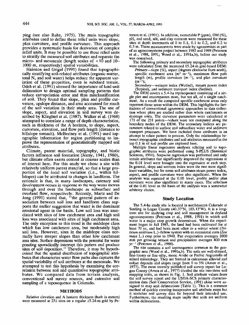
ping (see also Ruhe, 1975). The main topographicattributes used to define these relief units were slope,plan curvature, and profile curvature. This approachprovides a systematic basis for derivation of complexrelief units. It may be possible to use these relief unitsto stratify the measured soil attributes and separate themicro- and mesoscale (length scales of < 10 and 10-1000 m, respectively) spatial variabilities.

Hairston and Grigal (1991) found that topographi-cally stratifying soil-related attributes (organic matter,total N, and soil water) helps reduce the apparent var-iation of these properties, even in subdued terrain.Odeh et al. (1991) stressed the importance of land unitdelineation to design optimal sampling patterns thatreduce extrapolation error and thus misclassificationof soil. They found that slope, plan and profile cur-vature, upslope distance, and area accounted for muchof the soil variation in their study area. The use ofslope, aspect, and elevation in soil survey was de-scribed by Klingbiel et al. (1987). Walker et al. (1968)attempted to correlate a range of depth characteristics,such as thickness of the A horizon, to slope, aspect,curvature, elevation, and flow path length (distance tohillslope summit). McBratney et al. (1991) used top-ographic information for region partitioning to im-prove the representation of geostatistically mapped soilattributes.

Climate, parent material, topography, and bioticfactors influence soil formation (Jenny, 1941, 1980),but climate often exerts control at coarser scales thanof interest here. For this study we chose a site withrelatively uniform parent material, so that a large pro-portion of the local soil variation (i.e., within hil-Islopes) can be attributed to changes in landform. Therationale is that, in many landscapes, catenary soildevelopment occurs in response to the way water movesthrough and over the landscape as subsurface andoverland flow, respectively. Recently, Martz and DeJong (1991) stated that, "the general pattern of as-sociation between soil loss and landform class sup-ports the earlier suggestion that water is the dominanterosional agent in the basin. Low soil loss was asso-ciated with sites of low catchment area and high soilloss was associated with sites of high catchment area.The only exception to this trend is the midslope classwhich has low catchment area, but moderately highsoil loss. However, sites in the midslope class nor-mally have steeper slopes than other low catchmentarea sites. Surface depressions with the potential for waterponding sporadically interrupt this pattern and producesites of soil deposition." Therefore, it may be hypoth-esized that the spatial distribution of topographic attri-butes that characterize water flow paths also captures thespatial variability of soil attributes at the mesoscale. Weattempted to test this hypothesis by examining the cor-relation between soil and quantitative topographic attri-butes. We compared data from terrain analysis,conventional soil survey sources, and extensive soilsampling of a toposequence in Colorado.

METHODSRelative elevation and A horizon thickness (both in meters)

were measured at 231 sites on a regular 15.24-m grid by Pe-

terson et al. (1991). In addition, extractable P (ppm), OM (%),pH, and sand, silt, and clay contents were measured for thesesites at depth increments of 0 to 0.1, 0.1 to 0.2, and 0.2 to0.3 m. These measurements were made by agronomists as partof an agroecosystems project between 1985 and 1989 (Petersonet al., 1988, 1991; Wood et al.,. 1991a,b), before our studywas conceived.

The following primary and secondary topographic attributeswere calculated from the measured 15.24-m grid-based DEM:

Primary—slope (%), aspect (degrees clockwise from north),specific catchment area (m2 m-1), maximum flow pathlength (m), profile curvature (m-1), and plan curvature(m-1);Secondary—wetness index (Wetind), stream power index(Strpind), and sediment transport index (Sedind).

The DEM covers a 5.4-ha toposequence consisting of a sin-gle plot and encompasses most, but not all, of a single catch-ment. As a result the computed specific catchment areas onlyrepresent those areas within the DEM. This highlights the lim-itations of conventional agronomic approaches to data collec-tion where plots are studied rather than whole catchments ordrainage units. The curvature parameters were calculated at171 of the 231 points—values were not computed along theboundary nodes of the DEM. The secondary indices are pa-rameters related to surface and subsurface water and sedimenttransport processes. We have included these attributes in anattempt to relate pattern to process. Only the relationships be-tween topographic attributes and soil attributes measured in thetop 0.1 m of soil profile are explored here.

Multiple linear regression analyses relating soil to topo-graphic attributes were performed using S-PLUS (StatisticalSciences, 1991). Stepwise regression was performed and onlyterrain attributes that significantly improved the regressions atthe 0.01 level were brought into the regression at each step.In general, slope and wetness index were the two most signif-icant variables, but for some soil attributes steam power index,aspect, and profile curvature were also significant. When theanalysis was repeated at the 0.05 level, profile and/or plancurvature were also significant in many cases. The selectionof the 0.01 level as the basis of the analysis was a somewhatarbitrary choice.

Study LocationThe 5.4-ha study site is located in northeastern Colorado at

Sterling in Logan County (40.37°N, 103.13°W). It is a long-term site for studying crop and soil management in drylandagroecosystems (Peterson et al., 1988, 1991) in which soilwater is a major crop growth determinant. When the experi-ment began in fall 1985, the land had been cultivated for atleast 70 yr, and had been most often in a winter wheat (Tri-ticum aestivum L.)-fallow system with an occasional corn (Zeamays L.) crop prior to 1940. Pan evaporation averages 1000mm per growing season and precipitation averages 400 mmyr-1 (Peterson et al., 1988).

The site contains a soil toposequence common to the geo-graphic area (Wood et al., 1991a,bj. The soils are well-drained,fine-loamy or fine-silty, mesic Aridic or Pachic Argiustolls ofmixed mineralogy. They are formed in calcareous alluvial andeolian deposits and slopes range from 0 to 5% (Amen et al.,1977). The most recently published soil survey report for Lo-gan County (Amen et al., 1977) divided the site into three soilmapping units, as shown in Fig. 1. Soil attribute values fromthe soil survey report and the USDA-SCS primary character-ization data (Soil Conservation Service, 1991) alone were as-signed to map unit delineations (Table 1). This is a commonmethod of quickly creating inexpensive soil attribute maps butit stretches soil survey data far beyond their intended use.Furthermore, the resulting maps imply that soils are uniformwithin delineations.

MOORE ET AL.: SOIL ATTRIBUTE PREDICTION USING TERRAIN ANALYSIS 445

90

Fig. 1. Boundaries of the soil mapping units for the Sterling,CO, site. Mapping units shown are: 126, Weld; 92, Rango;and 90, Plantner. Fig. 2. Structure of a grid-based digital elevation model showing

a moving three by three submatrix centered on node 5.

Laboratory AnalysisSoil particle-size fractions were measured using the hydrom-

eter method after dispersal with sodium hexametaphosphate(Day, 1965). Soil extractable P and organic matter were de-termined using the standard NaHCO3 procedure and modifiedWalkley-Black method, respectively (Olsen and Sommers,1982; Schnitzer, 1982). The pH was measured in water usinga 1:1 soil/water ratio (McLean, 1982).

Calculating Topographic AttributesTopographic attributes can be divided into primary and sec-

ondary (or compound) attributes. Primary attributes are di-rectly calculated from a DEM and include variables such aselevation, slope, plan and profile curvature, flow path lengths,and specific catchment area. Compound attributes involvecombinations of the primary attributes and can be used to char-acterize the spatial variability of specific processes occurringin the landscape (Moore et al., 1991, 1993). These compoundattributes may be derived empirically, or by simplifying equa-tions describing the underlying physics of the processes. Top-ographic indices provide a knowledge-based approach to soil-specific management and analysis and can be imbedded withinthe data analysis subsystems of a GIS. Because many GISsare based on a pixel or raster structure (i.e., grid cell), grid-based methods of terrain analysis can provide the primary geo-graphic data for GIS applications.

A computationally efficient method of estimating primaryterrain attributes from a grid-based DEM applies a second-order, central finite-difference scheme centered on the interiornode of a moving three by three square grid network (Fig. 2).

The grid spacing of this network is A. We can simplify themathematics by using the following notation. Forward andbackwards difference schemes were used to handle nodes onthe edges of the DEM.

te f = & / = *J?'* ax' Jy ay' ;~ a*2'

lyyd2z

dxdy [1]

where z is the elevation, x and y are the orthogonal directionsin the horizontal plane, and

P = = P + [2]If Z is the node elevation shown in Fig. 2, then the centralfinite-difference forms of the partial derivatives for the centralnode 5 can be written as:

Z6 -Z42A '-Zj +

£ A

Z3 + Z7

4A2

Z2 - Z82A

-Z97

ZA + Zf. — 2Zc Z&- 2Z5

A2 [3]

Table 1. Soil attribute data estimated for map units in a cropped field near Sterling, CO.Sourcet

MMMSMMMMSSS

M,SSMM

AttributesMap unit numberLocationMapped as:Sampled as:DrainageRunoffSlope, mm-1 x 100A horizon depth, mOrganic C x 1.72, 0-0.1 m, g kg-1

Extr. P, 0-0.1 m, mg kg- 4Sand, 0-0.1 m, %pH (1:1), 0-0.3mBk horizon depth, mWater supply, rankYield, t/ha-^

126SummitWeldWeldwd

slow1-3

0.180.165

2745

6.6-7.80.51

intermediate1.7-4.0

90Side

PlantnerSatanta

wdmedium

3-50.180.155

1754

6.6-8.00.38lowest1.7-2.6

92Toe

RangoAlbinas

wdslow0-3

0.66110.220

4242

6.6-7.80.65highest2.0-3.7

126,90,92Whole field

Weld, Plantner, RangoWeld, Satanta, Albinas

wdslow-medium

0-50.18-0.66

0.155-0.22017-4242-546.6-8.0

0.38-0.65_

1.7^».0t M = map unit component data from soil survey report, Logan County, Colorado (Amen et al., 1977); S = soil samples from similar soils, Primary

Characterization Data (Soil Conservation Service, 1991)t NaHCOj-extractable P.§ Range in wheat yield potential is related to low or high management levels as defined by the USDA-SCS.H Includes buried A horizon materials with mollic colors.


The maximum slope, /3 (in degrees), aspect, iff (measuredin degrees clockwise from north), and curvature (m-1) of themidpoint in the moving grid can then be calculated using thefollowing relationships:

/3 = arctanO1/2),

iA = 180 — arctan + 901^1, andk|«>

curvature = , sin2</>cosv

[4]

where v is the angle between the normal to the surface and thesection plane and cf> is the angle between the tangent of thegiven normal section and the x axes (Kepr, 1969; Moore, 1990;Mitasova and Jaroslave, 1993). The two directions of mean-ingful curvature for hydrological and geomorphological appli-cations are in the direction of maximum slope (profile curvature)and transverse to this slope (plan curvature). Profile curvatureis a measure of the rate of change of the potential gradient andis therefore important for water flow and sediment transportprocesses; plan curvature is a measure of the convergence ordivergence and hence the concentration of water in a land-scape. For profile curvature, <p,

cosv = 1, cos<£ =

so that <p =

(pq)l

f f2 + 2f f f +JxxJ* J y

pq [5]

Similarly, for plan curvature, <u,

cosv = I - cos<£ = -^, and sin<£ = -^=P P

so that M = /«/? - + fyft [6]

The plan area in the horizontal plane characterized by eachnode or grid point is Ah = A2. Jenson and Domingue (1988)described a computationally efficient algorithm for estimatingflow directions and hence catchment areas and drainage pathlengths for each node in a regular grid DEM based on theconcept of a depressionless DEM. They assumed that waterflows from a given node (say node 5 in Fig. 2) to one of eightpossible neighboring nodes (nodes 1-4, 6-9 in Fig. 2), basedon the direction of steepest descent. Upslope flow paths com-puted using this algorithm tend to zigzag and therefore aresomewhat unrealistic. Moore et al. (1993) described a modi-fication of this algorithm that allows flow from one node (saynode 5) to be distributed to multiple nearest neighbor elementsin upland areas above defined channels on a slope-weightedbasis. This new algorithm allows flow divergence to be rep-resented in a grid-based method of analysis. The algorithm canbe combined with the above finite-difference approach to es-timate a wide variety of hydrologically significant topographicattributes.

Three hydrologically based compound indices that have po-tential use in predicting the spatial distribution of soil prop-erties and in soil-specific crop management are the wetnessindex, w, the stream power index, fi, and a sediment transportcapacity index, t (Moore et al., 1991). The wetness index hasbeen used to characterize the spatial distribution of zones ofsurface saturation and soil water content in landscapes (Moore

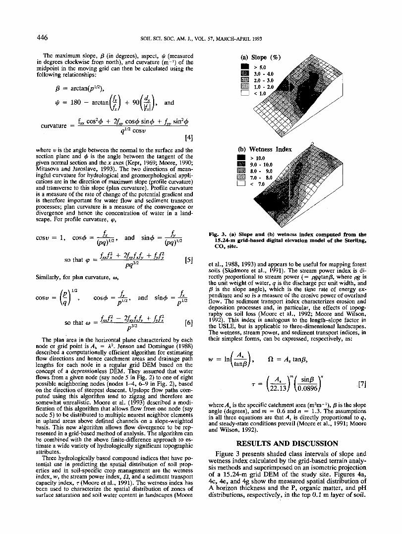
(a) Slope (%)

Fig. 3. (a) Slope and (b) wetness index computed from the15.24-m grid-based digital elevation model of the Sterling,CO, site.

et al., 1988,1993) and appears to be useful for mapping forestsoils (Skidmore et al., 1991). The stream power index is di-rectly proportional to stream power (= pgqlan/3, where pg isthe unit weight of water, q is the discharge per unit width, andP is the slope angle), which is the time rate of energy ex-penditure and so is a measure of the erosive power of overlandflow. The sediment transport index characterizes erosion anddeposition processes and, in particular, the effects of topog-raphy on soil loss (Moore et aL, 1992; Moore and Wilson,1992). This index is analogous to the length-slope factor inthe USLE, but is applicable to three-dimensional landscapes.The wetness, stream power, and sediment transport indices, intheir simplest forms, can be expressed, respectively, as:

w =tan/3

ft = As tan/3,

T = -V22.13/ VO.0896/ ms is the specific catchment area (nrta-1), j8 is the slope

angle (degrees), and m = 0.6 and n = 1.3. The assumptionsin all three equations are that As is directly proportional to q,and steady-state conditions prevail (Moore et al., 1991; Mooreand Wilson, 1992).

RESULTS AND DISCUSSIONFigure 3 presents shaded class intervals of slope and

wetness index calculated by the grid-based terrain analy-sis methods and superimposed on an isometric projectionof a 15.24-m grid DEM of the study site. Figures 4a,4c, 4e, and 4g show the measured spatial distribution ofA horizon thickness and the P, organic matter, and pHdistributions, respectively, in the top 0.1 m layer of soil.


(a) A Horizon (m)• > 0.40• 0.30 - 0.40Hi 0.20 - 0.30Hi 0.10 - 0.20EH < o.io

(b) Predicted A Horizon (m)• > 0.40• 0.30 - 0.40HI 0.20 - 0.30

0.10 - 0.20EH < o.io

(c) Phosphorus (mg kg"1)• > 21.0• 15.0 - 21.0IH 9.0 - 15.0

EH < 6.0

(d) Predicted Phosphorus (mg kg l)• > 21.0• 15.0 - 21.0• 9.0 - 15.0• 6.0 - 9.0EH < 6.0

(e) Organic Matter• > 2.00• 1.60 - 2.00

1.40 - 1.60ill 1.20 - 1.40EH < 1.20

(f) Predicted Organic Matter (%)• > 2.00• 1.60 - 2.00• 1.40 - 1.60

1*20 -EH < 1.20

(g) pH• > 8.00• 7.80 - 8.00IB! 7.40 - 7.80iJi 7.00 - 7.40.EH < 7.00

(h) Predicted pH• > 8.00• 7.80 - 8.00• 7.40 - 7.80

7.00 -EH < 7.00

7.40.

Fig. 4. Measured and predicted soil attributes at the Sterling, CO, site.

A horizons thicker than 0.25 m are mostly confinedto summit and toeslope positions where slopes are < 2%(Fig. 3a and 4a) and at or immediately downslope ofareas with the greatest concavity (profile curvature). Whereslopes steeper than 2% have thick A horizons, they areassociated with areas that have a wetness index >8.0(Fig. 3b). Here additional subsoil water has apparently

allowed greater root activity than in adjacent areas thatare just as steep but not so wet. To some extent the Ahorizon is a "fossil record" of root activity that reflectsthe redistribution of water by the terrain. Wetter areascould also have more vegetation cover and consequentlyless erosion. Thick A horizons in toeslope positions mayresult from the deposition of sediments carried in over-


A-hor 0.57 0.5 -0.36 0.6 -0.48 -0.64 0.16 0.55 -0.091 -0.39

0.6 -0.44 0.6 -0.45 -0.61 0.1 0.53 -0.14 -0.42

OM -0.11 0.6 -0.43 -0.45 -0.13 0.57 -0.0037 -0.23

PH -0.38 0.49 0.55 -0.51 -0.25 0.27 0.45

Silt •0.77 -0.63 0.13 0.61 -0.046 -0.33

I ••* It I 1.1*1 I . _: :!:::::::•• i• M-HCI i

•i;..I I I I I

Sand 0.64 -0.27 -0.45 0.19 0.42

Slope -0.33 -0.43 0.41 0.75

HI!-! fe I^ir Aspect 0.067 -0.23 -0.3

I • • ! •hi Wetind 0.45 0.06

iliifc Strpind 0.87

• • ' 'illilli! liiillii i-a '? Sedtind

Fig

5 10 20 5 15 25

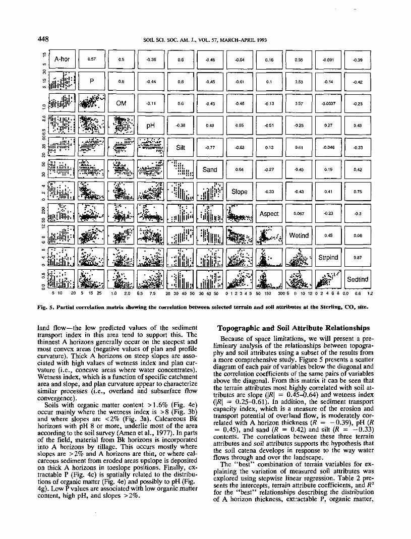
5. Partial correlation

1.0 2.0 6.5 7.5 20 30 40 50 30 40 50 0 1 2 3 4 5 50 150 300 6 8 10 12 0 2 4 6 8 0.0 0.6 1.2

matrix showing the correlation between selected terrain and soil attributes at the Sterling, CO, site.

land flow—the low predicted values of the sedimenttransport index in this area tend to support this. Thethinnest A horizons generally occur on the steepest andmost convex areas (negative values of plan and profilecurvature). Thick A horizons on steep slopes are asso-ciated with high values of wetness index and plan cur-vature (i.e., concave areas where water concentrates).Wetness index, which is a function of specific catchmentarea and slope, and plan curvature appear to characterizesimilar processes (i.e., overland and subsurface flowconvergence).

Soils with organic matter content >1.6% (Fig. 4e)occur mainly where the wetness index is >8 (Fig. 3b)and where slopes are <2% (Fig. 3a). Calcareous Bkhorizons with pH 8 or more, underlie most of the areaaccording to the soil survey (Amen et al., 1977). In partsof the field, material from Bk horizons is incorporatedinto A horizons by tillage. This occurs mostly whereslopes are > 2% and A horizons are thin, or where cal-careous sediment from eroded areas upslope is depositedon thick A horizons in toeslope positions. Finally, ex-tractable P (Fig. 4c) is spatially related to the distribu-tions of organic matter (Fig. 4e) and possibly to pH (Fig.4g). Low P values are associated with low organic mattercontent, high pH, and slopes >2%.

Topographic and Soil Attribute RelationshipsBecause of space limitations, we will present a pre-

liminary analysis of the relationships between topogra-phy and soil attributes using a subset of the results froma more comprehensive study. Figure 5 presents a scatterdiagram of each pair of variables below the diagonal andthe correlation coefficients of the same pairs of variablesabove the diagonal. From this matrix it can be seen thatthe terrain attributes most highly correlated with soil at-tributes are slope (\R\ = 0.45-0.64) and wetness index(\R\ = 0.25-0.61). In addition, the sediment transportcapacity index, which is a measure of the erosion andtransport potential of overland flow, is moderately cor-related with A horizon thickness (R = - 0.39), pH (R= 0.45), and sand (R = 0.42) and silt (R = -0.33)contents. The correlations between these three terrainattributes and soil attributes supports the hypothesis thatthe soil catena develops in response to the way waterflows through and over the landscape.

The "best" combination of terrain variables for ex-plaining the variation of measured soil attributes wasexplored using stepwise linear regression. Table 2 pre-sents the intercepts, terrain attribute coefficients, and R2

for the "best" relationships describing the distributionof A horizon thickness, extractable P, organic matter,


pH, and sand and silt contents in the top 0.1 m of thesoil profile. The numbers in parentheses indicate the or-der in which the variables were brought into the regres-sions. Only variables that improved the regressions atthe 0.01 level were included. In many cases, profile and/or plan curvature were significant variables at the 0.05level. These regression equations were then used to pre-dict the spatial distribution of A horizon thickness, ex-tractable P, organic matter, and pH. The predicted andmeasured values are compared in Fig. 4.

The regression equations presented in Table 2 ex-plain from 41 to 64% of the variability of measuredsoil attributes. We consider this to be quite good. Withhigher resolution and larger scale digital elevationmodels (5-m grid as opposed to the 15.24 m used here)that can characterize microscale (length scales of < 10m) variations in the terrain, it may be possible to ex-plain a higher proportion of the variance. Emergingtechnologies such as the GPS and other space- andaircraft-based methods may soon make this possible.However, because of the highly variable nature of soilattributes it is unrealistic to expect that the methodsproposed here could explain more than about 70% ofthe variance. Even pedotransfer functions that relatesoil textural properties to other soil attributes (e.g.,hydraulic conductivity) do not explain more of the var-iability than this. Traditionally, soil scientists have notincorporated information about local processes (suchas hydrology and soil erosion and deposition) in at-tempting to develop pedotransfer functions, and havenot been able to predict the spatial variability of soilattributes within soil map units. The optimum scalesfor studying and characterizing landscape processes af-fecting the development of the soil catena are unknownand represent a major research need (Moore et al.,1991).

The Sterling study site is a relatively small area andhas limited ranges of the computed terrain attributes,particularly aspect (mostly northerly). To extend themethods described above to larger and more heteroge-neous landscapes would require the introduction of ad-ditional descriptors including geology, stratigraphy,climate (precipitation and temperature), vegetation, andthe radiation regime. Human activities have altered mostsoil landscapes, and the record of that activity is in thecurrent stratigraphic record in the form of recently de-posited sediments. In future, soil sampling and analysiscould be better accomplished using a horizonation ap-proach. The radiation regime is characterized in part byslope-aspect interactions and is important in modifying

the soil water and evaporation distributions in land-scapes, and hence soil attributes and agronomic poten-tial. The spatial distribution of radiation can becharacterized using a relatively simple radiation index(see Moore et al., 1991, 1993) and becomes importantat higher latitudes. Hutchinson (1991) described efficientmethods of spatially interpolating monthly climatic dataon the basis of latitude, longitude, and elevation. Thesemethods could be used to provide the necessary data fora more extensive analysis aimed at predicting soil phys-ical and chemical properties. We believe that in moreheterogeneous landscapes the plan and profile curvaturesmay be more significant than reported here.

Surface soil properties are most modified by land man-agement. Therefore, features of lower horizons in theprofile may show greater response to topographic attri-butes (e.g., degree of leaching, distribution of Na, etc.).Also, the topography of the contact between the consol-idated and unconsolidated materials or the presence ofsedimentary features in the regolith may be significantin some landscapes.

Enhancing Soil Attribute Mapsfrom Soil Surveys

The estimated range in slope for the Sterling field,based on soil slope classes reported in the county soilsurvey (0-5%), is essentially identical to the range (0.1-5.2%) of the slope estimates from the DEM of the field.The soil survey here has provided an accurate range ofslope estimates for the field but the survey can be en-hanced with DEM data that can represent the distributionof terrain and soil attributes within soil survey map de-lineations.

In the following discussion we attempt to illustratehow enhanced soil attribute maps could be derived fromconventional soil survey sources using terrain attributesto spatially distribute soil attributes within a field or mapunit. If we assume that the range of soil attribute valuesfor a field is largely a function of terrain, the assignmentof values to grid cells according to slope position, wet-ness index, or other terrain attributes could be more re-alistic than assigning mean values based on the soil surveyalone. In other words, we can use the appropriate terrainattributes to scale the reported range of soil attribute val-ues to obtain spatially distributed estimates of soil attri-butes or soil attribute maps.

To demonstrate, in a simple way, how our proposedapproach can be expanded and applied, we assume that,

Table 2. Regression equations relating measured soil properties in the top 0.1 m to significant terrain attributes (P < 0.01).

Terrain attribute

Intercept of regressionAttributes

SlopeWetness indexStream power indexAspectfProfile curvature

P?

A horizondepth

m0.096

-0.053(l)t0.031(2)

-—-

0.503

Organicmatter

%0.285

-0.190(1)

-0.070(2)-0.002(3)

-0.482

ExtractableP

mgkg-'-3.039

-1.466(1)2.311(2)

-0.769(3)——

0.483

PH

7.508

0.190(1)--

-0.003(2)—

0.409

Sand———————— °/i

46.417

2.941(1)-1.320(2)

—-

27.592(3)0.517

Silt

23.466

-2.009(1)2.076(2)-—

-27.241(3)0.636

t Numbers in parentheses indicate the order in which the variables were brought in to the regressions.t Aspect measured in degrees clockwise from west.


as a first approximation, soil attributes are linearly re-lated to terrain attributes. With this assumption, eitherof the following relationships can be used to predict thespatial distribution of soil properties:

(a) A Horizon Predicted from Soil Survey (m)

/P /i,min

or

ip /i.min

\r,,max - 7,,min)

T — TAk •ifr,~~ ~

n /TV //,max fi,min) 2^ \ \ -*•*=i \ L

- T*£[8b]

where yp is the predicted soil attribute at the point ofinterest, A, max and A/)min are the maximum and minimumvalues of the soil attribute in the field or mapping unit i(from soil survey), fik is a weighting coefficient for ter-rain attribute k (S/j, = 1), Tk is the value of the fcthterrain attribute at the point of interest, Tk>max and Tk minare the maximum and minimum values of the terrainattribute in the field or mapping unit i, and n is thenumber of terrain attributes used in the analysis. Equa-tion [8a] is used for positively correlated variables andEq. [8b] for negatively correlated variables. The valuesof the weighting coefficients could be assigned in a num-ber of ways, but might, for instance, be set proportionalto the fraction of the total variance explained by eachvariable.

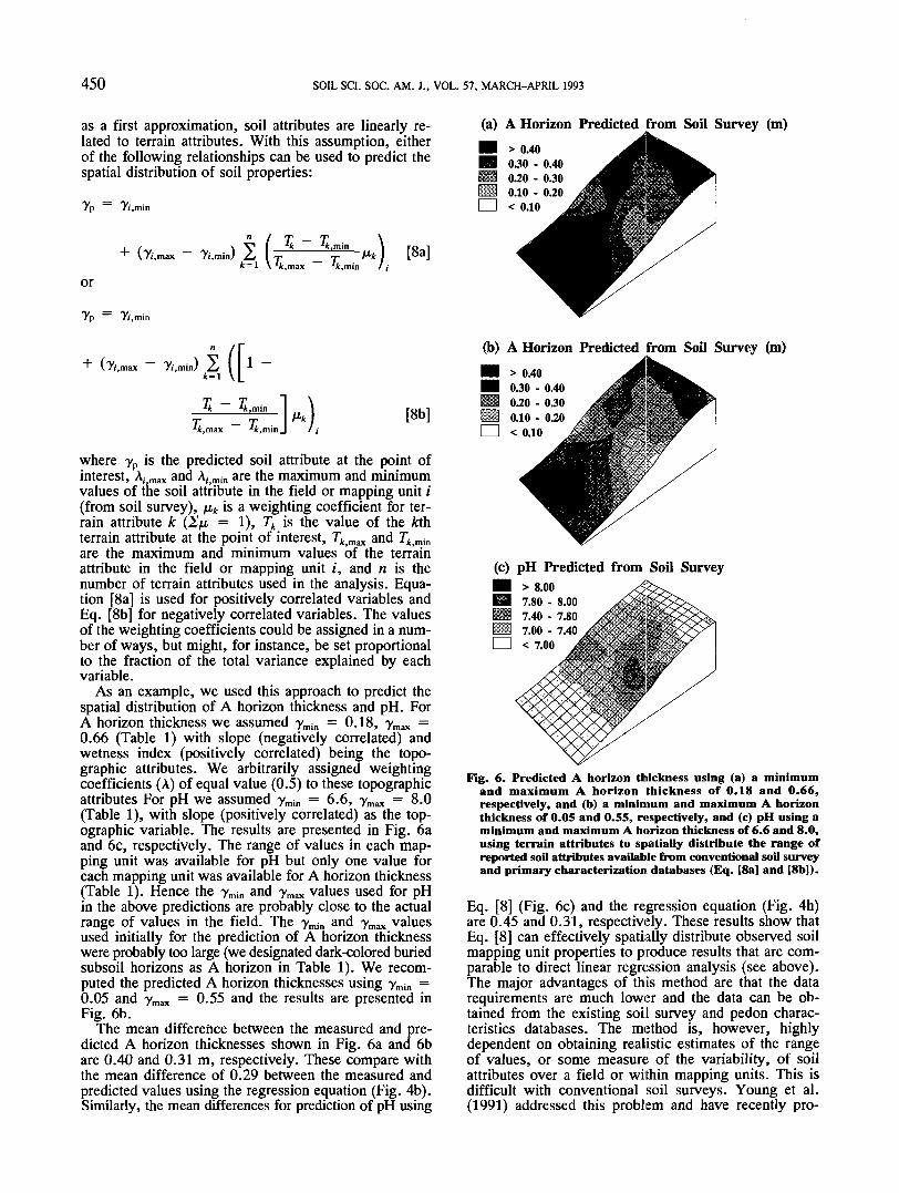
As an example, we used this approach to predict thespatial distribution of A horizon thickness and pH. ForA horizon thickness we assumed ymin = 0.18, ymax =0.66 (Table 1) with slope (negatively correlated) andwetness index (positively correlated) being the topo-graphic attributes. We arbitrarily assigned weightingcoefficients (A) of equal value (0.5) to these topographicattributes For pH we assumed ymin = 6.6, ymax = 8.0(Table 1), with slope (positively correlated) as the top-ographic variable. The results are presented in Fig. 6aand 6c, respectively. The range of values in each map-ping unit was available for pH but only one value foreach mapping unit was available for A horizon thickness(Table 1). Hence the ymin and ymax values used for pHin the above predictions are probably close to the actualrange of values in the field. The -ymin and ymax valuesused initially for the prediction of A horizon thicknesswere probably too large (we designated dark-colored buriedsubsoil horizons as A horizon in Table 1). We recom-puted the predicted A horizon thicknesses using ymin =0.05 and -ymax = 0.55 and the results are presented inFig. 6b.

The mean difference between the measured and pre-dicted A horizon thicknesses shown in Fig. 6a and 6bare 0.40 and 0.31 m, respectively. These compare withthe mean difference of 0.29 between the measured andpredicted values using the regression equation (Fig. 4b).Similarly, the mean differences for prediction of pH using

• > 0.40B 0.30 - 0.40• 0.20 - 0.30

0.10 - 0.20EH < 0.10

(b) A Horizon Predicted from Soil Survey (m)• > 0.40• 0.30 - 0.40• 0.20 - 0.30111 0.10 - 0.20cm < 0.10

(c) pH Predicted from Soil Survey• > 8.00B 7.80 - 8.00• 7.40 - 7.80

7 00 - 'LI] < 7.00

7.40

Fig. 6. Predicted A horizon thickness using (a) a minimumand maximum A horizon thickness of 0.18 and 0.66,respectively, and (b) a minimum and maximum A horizonthickness of 0.05 and 0.55, respectively, and (c) pH using aminimum and maximum A horizon thickness of 6.6 and 8.0,using terrain attributes to spatially distribute the range ofreported soil attributes available from conventional soil surveyand primary characterization databases (Eq. [8a] and [8b]).

Eq. [8] (Fig. 6c) and the regression equation (Fig. 4h)are 0.45 and 0.31, respectively. These results show thatEq. [8] can effectively spatially distribute observed soilmapping unit properties to produce results that are com-parable to direct linear regression analysis (see above).The major advantages of this method are that the datarequirements are much lower and the data can be ob-tained from the existing soil survey and pedon charac-teristics databases. The method is, however, highlydependent on obtaining realistic estimates of the rangeof values, or some measure of the variability, of soilattributes over a field or within mapping units. This isdifficult with conventional soil surveys. Young et al.(1991) addressed this problem and have recently pro-


posed specific field sampling methods for developingconfidence intervals for soil attributes within mappingunits.

Another potential method for spatially distributing soilattributes is to use terrain attributes to segment the land-scape into essentially stationary process zones where at-tribute prediction may be done in a more statisticallyrobust fashion. Dikau (1989) demonstrated one possiblesegmentation based on plan and profile curvature.

SUMMARY AND CONCLUSIONSTerrain modifies the distribution of hydrologic and

erosional processes (i.e., soil water content, runoff andsedimentation) and soil temperature in fields. Terrainthereby affects the distributions of mineral weathering,leaching, erosion, sedimentation, decomposition, hori-zonation, and, ultimately, soil attributes. Soil survey mapsand databases are readily available sources of estimatedsoil attribute data. However, the map resolution is gen-erally inadequate for soil-specific management and de-tailed environmental modeling. Data from these sourcescan be enhanced using terrain attributes (computed fromhigh-resolution OEMs) to spatially distribute estimatedsoil attribute data. These methods offer a promising, cost-effective means of creating the high-resolution mapsneeded for soil-specific crop management. They also al-low existing basic data sets (e.g., soil survey primarycharacterization data) to continue to be used as new tech-niques and technologies develop. Using GIS to organizeand build on these data sets will improve our knowledgeof environmental processes and promote economical andsustainable land management.

Results indicate that significant correlations betweenquantified terrain attributes and measured soil attributesexist. Slope and wetness index were the terrain attributesmost highly correlated with soil attributes measured at231 locations in a 5.4-ha toposequence in Colorado. In-dividually, they accounted for about one-half of the var-iability of several soil attributes including A horizonthickness, organic matter content, pH, extractable P, andsilt and sand contents. This represents an incorporationof finer scale process-based information relating to soilformation patterns in the landscape. A method is pre-sented to illustrate how relationships between terrain andsoil attributes may be used to enhance an existing soilmap, even when the exact form of the relationship isunknown. Other methods such as cokriging (which re-quires an estimate of the variogram) or partial splinesmay prove a viable alternative, although they generallyrequire a large number of data points. However, if dif-ferent soil attributes have different variograms, the idealsampling sites for the different attributes might not co-incide with one another. Terrain-based techniques mayalso be applied as a first step to guide sampling andmodel development in unmapped areas.

In applying Eq. [8] some a priori knowledge of ca-tenary sequences is needed (e.g., organic matter contentincreases downslope, base status is lower in wet areas,etc.). The underlying pedological or catenary models areusually developed during a soil survey but they are oftenreported only as verbal models, if at all. If the procedureis to be implemented, then survey practice must changeso that these verbal models are presented explicitly andconsistently. If this could be achieved, then more of the

surveyor's knowledge could be transferred than has hith-erto been possible. We have attempted to outline oneform that this quantitative framework might take.

Soil scientists and agronomists need to begin lookingat whole catchments or drainage units, rather than indi-vidual plots. The results presented here show that, inparticular, the hydrology of the catchment area outsideof the plot has a significant impact on the soil attributesand, therefore, crop production potential of the plot.

ACKNOWLEDGMENTSThis study was funded in part by Grant no. NRMS-M218

from the Murray-Darling Basin Commission; Grant no. 90/6334 from the Australian Department of Industry, Technologyand Commerce, Bilateral Science and Technology Program,the Water Research Foundation of Australia; and USDA-CSRSGrant no. 290684 from the PLACES Industrial Affiliates Pro-gram and the USDA-ARS Great Plains Systems Unit. Theauthors thank Dr. Dwayne G. Westfall of the Department ofAgronomy, Colorado State University, for the elevation andsoil attribute data from the Sterling, CO, site. Many sugges-tions and comments from Dr. Neil McKenzie and Dr. KevinMcSweeney have been incorporated into this paper and theauthors acknowledge their contribution.


ERRATA

Soil Attribute Prediction Using Terrain AnalysisI.D. MOORE, P.E. GESSLER, G.A. NIELSEN, AND G.A. PETERSONSoil Sci. Soc. Am. J. 57:443-452 (March-April 1993)

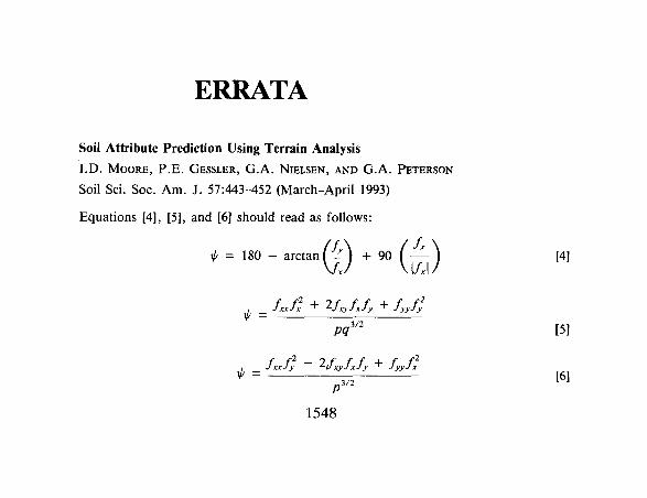
Equations [4], [5], and [6] should read as follows:

-,»-.«. (£)+., (A) ,4]

, _ JxxJx ~"~ ^JxyJxJy ' JyyJy

, _ JxxJy ~ ^JxyJxJy ' JyyJx•

1548

15]

Documents

Soil Attribute Prediction Using Terrain Analysis