University of Texas at El PasoDigitalCommons@UTEP

Open Access Theses & Dissertations

2014-01-01

Solar PV Power Generation Forecasting UsingHybrid Intelligent Algorithms and UncertaintyQuantification Based on Bootstrap ConfidenceIntervalsDonna AlhakeemUniversity of Texas at El Paso, dialhakeem@miners.utep.edu

Follow this and additional works at: https://digitalcommons.utep.edu/open_etdPart of the Economics Commons, Engineering Commons, and the Oil, Gas, and Energy

Commons

This is brought to you for free and open access by DigitalCommons@UTEP. It has been accepted for inclusion in Open Access Theses & Dissertationsby an authorized administrator of DigitalCommons@UTEP. For more information, please contact lweber@utep.edu.

Recommended CitationAlhakeem, Donna, "Solar PV Power Generation Forecasting Using Hybrid Intelligent Algorithms and Uncertainty QuantificationBased on Bootstrap Confidence Intervals" (2014). Open Access Theses & Dissertations. 1191.https://digitalcommons.utep.edu/open_etd/1191

SOLAR PV POWER GENERATION FORECASTING USING HYBRID

INTELLIGENT ALGORITHMS AND UNCERTAINTY

QUANTIFICATION BASED ON BOOTSTRAP

CONFIDENCE INTERVALS

DONNA IBRAHIM ALHAKEEM

Department of Electrical and Computer Engineering

APPROVED:

Paras Mandal, Ph.D., Chair

Tzu-Liang (Bill) Tseng, Ph.D. Co-Chair

Virgilio Gonzalez, Ph.D.

Charles Ambler, Ph.D.

Dean of the Graduate School

Copyright ©

by

Donna Ibrahim AlHakeem

2014

SOLAR PV POWER GENERATION FORECASTING USING HYBRID

INTELLIGENT ALGORITHMS AND UNCERTAINTY

QUANTIFICATION BASED ON BOOTSTRAP

CONFIDENCE INTERVALS

by

DONNA IBRAHIM ALHAKEEM, Bachelor of Science in Electrical Engineering

THESIS

Presented to the Faculty of the Graduate School of

The University of Texas at El Paso

in Partial Fulfillment

of the Requirements

for the Degree of

MASTER OF SCIENCE

Department of Electrical and Computer Engineering

THE UNIVERSITY OF TEXAS AT EL PASO

December 2014

iv

Acknowledgements

I would like to express my utmost gratitude to Dr. Paras Mandal as my thesis professor

for his guidance, mentoring and contribution through the process of my thesis and research

career. Without his input, I could not have finished this work. I would like to thank Dr. Bill

Tseng, Co-Chair, for this thesis as well as his guidance and support throughout my research

career. I would also like to thank Dr. Virgilio Gonzalez as a thesis committee member. I would

like to show appreciation to the Electrical and Computer Engineering department chair, Dr.

Miguel Velez-Reyes, for providing financial support to present my work at the North American

Power Symposium 2013 conference that was in Manhattan, KS. I would like to recognize Dr.

Ashraf Ul Haque for his guidance in this work. I would like to express my gratitude to the U.S.

Department of Education – DHSIP Program (Award #P031S120131) for partially funding this

study.

v

Abstract

This thesis focuses on short-term photovoltaic forecasting (STPVF) for the power

generation of a solar PV system using probabilistic forecasts and deterministic forecasts.

Uncertainty estimation, in the form of a probabilistic forecast, is emphasized in this thesis to

quantify the uncertainties of the deterministic forecasts. Two hybrid intelligent models are

proposed in two separate chapters to perform the STPVF. In Chapter 4, the framework of the

deterministic proposed hybrid intelligent model is presented, which is a combination of wavelet

transform (WT) that is a data filtering technique and a soft computing model (SCM) that is

generalized regression neural network (GRNN). Additionally, this chapter proposes a model that

is combined as WT+GRNN and is utilized to conduct the forecast of two random days in each

season for 1-hour-ahead to find the power generation. The forecasts are analyzed utilizing

accuracy measures equations to determine the model performance and compared with another

SCM. In Chapter 5, the framework of the proposed model is presented, which is a combination

of WT, a SCM based on radial basis function neural network (RBFNN), and a population-based

stochastic particle swarm optimization (PSO). Chapter 5 proposes a model combined as a

deterministic approach that is represented as WT+RBFNN+PSO, and then a probabilistic

forecast is conducted utilizing bootstrap confidence intervals to quantify uncertainty from the

output of WT+RBFNN+PSO. In Chapter 5, the forecasts are conducted by furthering the tests

done in Chapter 4. Chapter 5 forecasts the power generation of two random days in each season

for 1-hour-ahead, 3-hour-ahead, and 6-hour-ahead. Additionally, different types of days were

also forecasted in each season such as a sunny day (SD), cloudy day (CD), and a rainy day (RD).

These forecasts were further analyzed using accuracy measures equations, variance and

uncertainty estimation. The literature that is provided supports that the proposed hybrid

intelligent model, WT+RBFNN+PSO, and the uncertainty estimation method bootstrap

confidence intervals are a new application for STPVF power generation, thus establishing this

thesis as innovative work.

vi

Table of Contents

Acknowledgements ....................................................................................................................... iiv

Abstract ............................................................................................................................................v

Table of Contents ........................................................................................................................... vi

List of Tables ................................................................................................................................. ix

List of Figures ..................................................................................................................................x

Chapter 1: Introduction ....................................................................................................................1

1.1 Background and Research Motivation ...........................................................................1

1.2 Statement Problem and Rationale for the Study ............................................................4

1.3 Objectives of the Thesis .................................................................................................6

1.4 Scope and Limitation .....................................................................................................6

1.5 Organization of the Thesis .............................................................................................8

Chapter 2: Literature Review .........................................................................................................10

2.1 Introduction ..................................................................................................................10

2.2 Solar and Wind as Variable Renewable Energy Resources .........................................10

2.2.1 Deterministic Solar Power Forecasting ....................................................................10

2.2.2 Deterministic Wind Power Forecasting ....................................................................12

2.2.3 Uncertainty Quantification in the Form of Probabilitic Forecasts ............................12

2.4 Factors Impacting Solar PV Power Forecasting ..........................................................13

2.5 Importance of Solar PV Power Forecasting.................................................................15

2.6 Summary ......................................................................................................................16

Chapter 3: Forecasting Models ......................................................................................................17

3.1 Introduction ..................................................................................................................17

3.2 Data Filtering Technique .............................................................................................17

3.3 Soft Computing Models ...............................................................................................18

3.4 Optimizations Techniques in Forecasting ....................................................................20

vii

3.4.1 Genetic Algorithm ....................................................................................................20

3.4.2 Particle Swarm Optimization ....................................................................................21

3.5 Probabilistic Models ....................................................................................................23

3.6 Summary ......................................................................................................................24

Chapter 4: Applying Wavelets to Predict Solar PV Power Output Using Generalized Regression

Neural Network.....................................................................................................................26

4.1 Introduction ..................................................................................................................26

4.2 Input Data.....................................................................................................................26

4.3 Proposed Hybrid Intelligent Forecasting Framework ..................................................27

4.4 Results and Discussion ................................................................................................28

4.4.1 Forecasting Accuracy Measures ...............................................................................28

4.4.2 One-Hour-Ahead Forecasting Results ......................................................................29

4.5 Summary ......................................................................................................................31

Chapter 5: Uncertainties Quantification of Solar PV Power Forecasts Using Bootstrap

Confidence Intervals .............................................................................................................32

5.1 Introduction ..................................................................................................................32

5.2 Input Data.....................................................................................................................32

5.3 Proposed Hybrid Intelligent Forecasting Framework ..................................................33

5.4 Simulation Results and Discussion ..............................................................................35

5.4.1 Forecasting Accuracy Measures ...............................................................................35

5.4.2 Solar PV Power Forecasting Results for Various Forecasting Horizons ................36

5.4.2.1 One-Hour-Ahead Solar PV Power Forecasting Results .....................................36

5.4.2.2 Three-Hour-Ahead Solar PV Power Forecasting Results ...................................39

5.4.2.3 Six-Hour-Ahead Solar PV Power Forecasting Results .......................................40

5.4.3 Forecasting Results for Sunny Days, Cloudy Days, and Rainy Days .....................41

5.4.3.1 One-Hour-Ahead Forecasting Results for Sunny Days, Cloudy Days, and Rainy

Days ............................................................................................................................42

viii

5.4.3.2 Three-Hour-Ahead Forecasting Results for Sunny Days, Cloudy Days, and

Rainy Days ...................................................................................................................43

5.4.3.3 Six-Hour-Ahead Forecasting Results for Sunny Days, Cloudy Days, and Rainy

Days .............................................................................................................................45

5.4.3.4 One-Hour-Ahead Forecasting Variance Results for Sunny Days, Cloudy Days,

and Rainy Days ...........................................................................................................46

5.4.3.5 Three-Hour-Ahead Forecasting Variance Results for Sunny Days, Cloudy Days,

and Rainy Days ............................................................................................................47

5.4.3.6 Six-Hour-Ahead Forecasting Variance Results for Sunny Days, Cloudy Days,

and Rainy Days ............................................................................................................48

5.4.4 Uncertainty Quantification of Solar PV Power Forecasting Using Bootstrap

Confidence Intervals .................................................................................................48

5.5 Summary ......................................................................................................................53

Chapter 6: Conclusions and Recommendations for Future Work .................................................54

6.1 General .........................................................................................................................54

6.2 Summary and Conclusions ..........................................................................................54

6.3 Contributions................................................................................................................55

6.4 Recommendation for Future Work ..............................................................................56

References ......................................................................................................................................57

Appendix I .....................................................................................................................................63

Appendix II ....................................................................................................................................67

Appdendix III .................................................................................................................................71

Appdendix IV.................................................................................................................................73

Vita ..............................................................................................................................................74

ix

List of Tables

Table 4.1: Comparison of forecasting performance of the proposed hybrid WT+GRNN

intelligent model with other models ............................................................................................. 30

Table 5.1: Randomly chosen forecasting days. ............................................................................ 36

Table 5.2: One-hour-ahead forecasting performance of WT+ RBFNN+PSO model with other

models ........................................................................................................................................... 37

Table 5.3: Three-hour-ahead forecasting performance of the proposed model with other models

....................................................................................................................................................... 40

Table 5.4: Six-hour-ahead forecasting performance of the proposed model with other models .. 41

Table 5.5: Selected SDs, CDs, and RDs in different seasons ....................................................... 42

Table 5.6: One-hour-ahead forecasting performance of hybrid models in winter and fall ........... 42

Table 5.7: One-hour-ahead forecasting performance of hybrid models in summer and spring ... 43

Table 5.8: Three-hour-ahead forecasting performance of hybrid models in winter and fall ........ 44

Table 5.9: Three-hour-ahead forecasting performance of hybrid models in summer and spring. 44

Table 5.10: Six-hour-ahead forecasting performance of hybrid models in winter and fall .......... 45

Table 5.11: Six-hour-ahead forecasting performance of hybrid models in summer and spring... 45

Table 5.12: Variance for one-hour-ahead forecasting .................................................................. 46

Table 5.13: Variance for three-hour-ahead forecasting ................................................................ 47

Table 5.14: Variance for six-hour-ahead forecasting ................................................................... 48

Table AI.1: Input parameters for any models that used BPNN, GRNN, and RBFNN ................. 63

Table AI.2: Input time parameters for Tables 5.2-5.4 .................................................................. 64

Table AI.3: Input time parameters for Tables 5.6-5.14 ................................................................ 65

Table AI.4: GA input parameters for solar PV forecasts .............................................................. 66

Table AI.5: PSO input parameters for solar PV forecasts ............................................................ 66

Table AIV.1: PC technical specifications and details ................................................................... 73

x

List of Figures

Figure 1.1: Capacity of solar PV by classification ......................................................................... 1

Figure 1.2: Example of a point forecast .......................................................................................... 3

Figure 1.3: Example of probabilisitic forecasting........................................................................... 3

Figure 1.4: Hourly non-stationary power output of a 15 kW PV system in Ashland, Oregon ....... 5

Figure 2.1: Effects of energy prices caused by solar PV in Texas ............................................... 15

Figure 3.1: Wavelet decomposition and reconstruction process .................................................. 18

Figure 3.2: A general architecture of a neural network ................................................................ 19

Figure 3.3: GA process model ...................................................................................................... 21

Figure 3.4: PSO algorithm process model .................................................................................... 22

Figure 4.1: Proposed deterministic hybrid WT+GRNN intelligent model for STPVF ................ 27

Figure 4.2: MAPE histogram comparing performances of the SCMs and hybrid models ........... 30

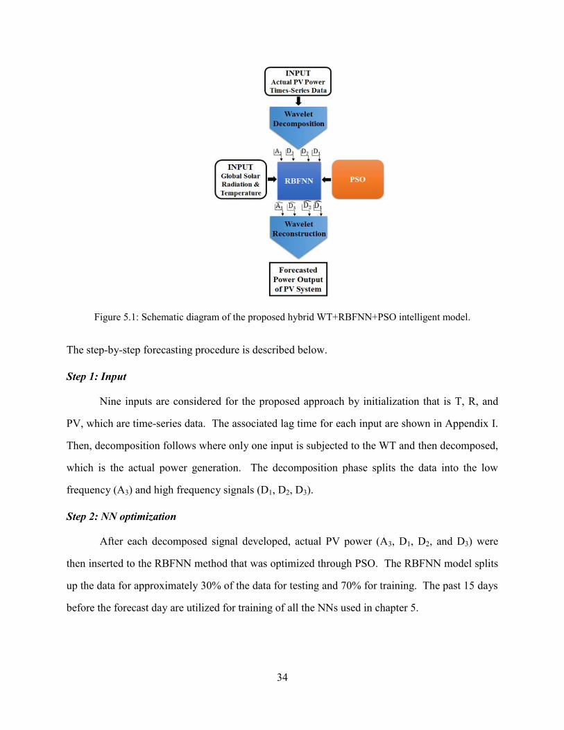
Figure 5.1: Schematic diagram of the proposed hybrid WT+RBFNN+PSO intelligent model ... 34

Figure 5.2: Comparison of the actual power generation and forecasted solar PV power using

WT+RBFNN+PSO ....................................................................................................................... 38

Figure 5.3: Comparison of the forecasting performance of the proposed WT+RBFNN+PSO

model with WT+GRNN+PSO ...................................................................................................... 39

Figure 5.4: Model WT+GRNN+GA in winter with a 95% confidence ........................................ 49

Figure 5.5: Model WT+GRNN+PSO in winter with a 95% confidence ...................................... 49

Figure 5.6: Model WT+RBFNN+GA in winter with a 95% confidence ...................................... 50

Figure 5.7: Model WT+RBFNN+PSO in winter with a 95% confidence .................................... 50

Figure 5.8: Model WT+GRNN+PSO in winter with a 95% confidence ...................................... 51

Figure 5.9: Model WT+RBFNN+PSO in winter with a 95% confidence .................................... 51

Figure 5.10: Bootstrap method for uncertainty estimation at 10%-90% confidence .................... 52

1

Chapter 1: Introduction

1.1 BACKGROUND AND RESEARCH MOTIVATION

There have been various technological changes that have occurred over recent years and

the behavior of the power grid is also evolving. Moreover, there have been increases of variable

energy resources (VERs), mainly solar and wind based technology, integrated to the power grid.

In addition, the integration of solar photovoltaic (PV) panels has been an alternative as an ideal

solution to distributed power generation. Residential and commercial solar PV installations yield

as a class majority of grid integrated PV capacity as shown in Figure 1.1. For the U.S., the total

solar PV capacity has nearly doubled in past recent years from approximately 1,900 MW in 2010

to 3,500 MW in 2011 [1]. People are observing the benefits of utilizing solar PV power since it

is a way to produce clean energy, reduce carbon footprint, and lower their electricity bill.

However, there are drawbacks to integrating solar PV technology that is due to day light

limitations and uncertainties such as weather variations, especially days that are cloudy or rainy

type days. These limitations such as the clouds prevent or cause these variations to the solar PV

systems, which are completely dependent on the sunlight.

Figure 1.1: Capacity of solar PV by classification.

MW

2

The electric utilities must now consider the changes that are occurring since their main

objective is to provide an efficient and reliable power to the end-user. In order to conduct

operations in a secure, efficient and economical way, there has to be an effective plan and set of

procedures to support it. This includes scheduling and forecasting while ensuring reliability.

The major power systems forecasting problems are associated with load demand forecasting,

solar PV power generation forecasting, wind power forecasting, wind speed forecasting, and

electricity price forecasting, which power utilities can forecast on short-term, medium-term, and

a long-term scale. Power utilities typically forecast on a long-term scale and now, recent

observations made by the power system utilities are noting that there is a need to develop a more

accurate and efficient short-term PV forecasting (STPVF) tool to predict the power generation of

a solar PV system in order to operate the power system more efficiently while maintaining the

security and reliability of the system [2]. In a short-term forecast, the hours to forecast can range

from hour-ahead to 1-week-ahead.

There are two forms of forecasting, which is point forecasting and probabilistic

forecasting. An example graph of what a point forecast would look like is presented in Figure

1.2 in which the blue line indicates the true value and the red dotted line indicates the forecasted

values. In a point forecast, the predicted value is produced as a particular value as an output,

which is also referred to as a deterministic forecast. In a deterministic forecast, the future values

of solar PV power generation is predicted providing a foundation for a probabilistic forecast,

respectively. In Figure 1.3, an example of a probabilistic forecast is graphed in which the solid

black line indicates the true value, the black dots indicate the forecasted values, and the green

upper and lower lines represent a range that is the probabilistic forecast. Various statistical time-

series models such as generalized auto-regressive heteroskedastic (GARCH) and auto-regressive

integrated moving average (ARIMA) models have been applied to a deterministic forecast.

Additionally, the time-series models are good when the frequency of data is low. However, they

can be very problematic when the frequency of data is very high and non-linear [3]. This thesis

presents the application of soft computing models (SCMs), which are artificial intelligence type

3

techniques, i.e., artificial neural networks (NNs). NNs are useful learning models that have the

advantage of dealing with non-linearity and complex problems [4]. A deterministic forecast can

be enhanced by quantifying uncertainty, i.e., a technique to quantify uncertainty associated with

solar PV forecasts can assist the deterministic forecast to distinguish uncertainty [5]. Uncertainty

quantification is best represented in the form of probabilistic forecasts [6]. Additionally, a range

of estimates from the probabilistic forecast will further enhance the deterministic forecast

through analysis and provide a more efficient conclusive decision on the deterministic forecast

models, such as SCMs. The reliability of the methodology will also improve by optimizing

certain parameters in SCMs, thus giving it more credibility.

Figure 1.2: Example of a point forecast.

Figure 1.3: Example of probabilistic forecasting.

4

1.2 STATEMENT PROBLEM AND RATIONALE FOR THE STUDY

Solar PV distributed generation and utility scale generation is increasing that has caused a

shift in the electric utilities traditional planning process of power generation while not being

equipped with an efficient method to forecast the solar PV power generation, thus producing an

uneconomical balance of the power systems operations. Effectively planning power generation

is an important function of a power utility company, particularly forecasting. As the power grid

evolves and grows, planning and procedures must adjust accordingly for these changes.

Consequently, more consideration must be focused on solar PV power generation as another

factor that must be accounted for by forecasting the solar power output of a PV system. To

pursue this economical operation, a more accurate forecasting technique must be applied to

predict the power generation of a solar PV system. There are many reasons that an accurate solar

PV power forecasting method is significant, which must become part of the planning process. A

recent policy, i.e. Regional Greenhouse Gas Initiative (RGGI), imposed on electric power plants

utilizing fossil fuels and having a capacity of more than 25 MW set a limitation of CO2

emissions [7]. Now, power utilities must respond to these enforcements to integrate renewables

into their grid through means of adding to their current installed capacity or providing incentives

for distributed generation. Within the next couple of years, the U.S. Energy Information

Administration (EIA) projects that PV and wind technologies will double in generation capacity

[8]. This increased penetration provides the necessity of an improved solar PV forecasting

method as this is not a highly saturated area of study [9]. In addition to confirm whether a

forecast is a legitimate one, accuracy measurements of the forecast and the uncertainty of the

forecast must be determined, which the electric power system operators observes as an important

[9].

There are various challenges that can affect solar PV power output forecasts such as, the

state of the environment, time of the day, and temperature. Weather is known to be intermittent

and a suddenly large unexpected variation can negate a forecast. For example, power generation

over the course of one month, March 2011, is presented in Figure 1.4 using the data acquired

5

from a 15 kW PV system located in Ashland, Oregon [10]. As it can be seen in Figure 1.4, the

generated solar PV power output is variable, non-stationary, and chaotic in nature. Since the

solar PV system is primarily dependent on the solar energy emitted from the sun, any obstruction

will impede solar power generation. The solar irradiation that is blocked by cloud cover

Figure 1.4: Hourly non-stationary power output of a 15 kW PV system in Ashland, Oregon.

affecting power production and is a factor that most solar PV forecasters observe as a challenge

in forecasting [11]. Solar PV forecasting can be difficult, which is due to these above-mentioned

challenges compromising power system reliability and the forecast will be not as predicted. That

is the reason why an improved or accurate method to forecast can prevent reliability issues of the

power system and avoid economic related losses [11]. In addition to these challenges, there is

not an abundance of research conducted regarding methods in STPVF. Motivated by the

aforementioned challenges, this thesis contributes to the development of deterministic hybrid

intelligent models to improve the short-term forecasting accuracy of solar PV power generation

and confidence interval estimation based on bootstrap method. The enhancement in forecasting

accuracy would be highly beneficial to the power system operators such as efficient planning and

operations.

6

1.3 OBJECTIVES OF THE THESIS

This thesis aims to develop intelligent forecasting and optimization methods for power

and renewable energy systems forecasting problems in order to improve the reliability and

performance of the electric power grid in the path towards a sustainable future. The specific

objectives of this thesis are:

Objective 1: To develop more efficient, accurate, and practical deterministic STPVF

model using hybrid intelligent algorithms.

- The objective-1 will involve the development of hybrid intelligent solar PV

power forecasting model that uses the combination of a data filtering technique based

on wavelet transform (WT), a soft computing model (SCM) based on generalized

regression neural network (GRNN), which is optimized by a stochastic population based

optimization algorithm.

Objective 2: To develop a new approach in order to quantify uncertainty estimation of

the solar PV power output in the form of probabilistic forecasts.

- The objective-2 will apply bootstrap confidence intervals to quantify uncertainty

estimation from the deterministic forecast involving the development of hybrid

intelligent solar PV power forecasting model that uses the combination of a data

filtering technique based on WT, a SCM based on radial basis function neural

network (RBFNN), which is optimized by a stochastic population based particle

swarm optimization (PSO) algorithm.

1.4 SCOPE AND LIMITATION

The study focuses on a hybrid intelligent technique using NN in order to forecast short-

term power output of a PV system. To demonstrate the superiority of the proposed method,

publicly available data acquired from the University of Oregon, Solar Radiation Monitoring

Laboratory website are used for training and testing the NN. Several methods are tested and

compared in this thesis to find a robust intelligent model.

7

The major scope of this thesis are the advantages of solar PV forecasting. Solar

forecasting will be beneficial to the power utilities in numerous ways considering the increasing

integration of renewables, particularly solar PV, into the power grid. By allowing the power

system utilities to be able to predict the solar power generation that is expected, the power

utilities can plan their traditional power production accordingly to account for when there is

enough or insufficient power being produced from the solar PV systems. The environment will

also benefit from solar PV forecasting by utilizing the solar irradiation to produce clean power

rather than alternative traditional power generating resources that can produce harmful emission

and a larger carbon footprint. Power system security will also be enhanced by improving

economical operation and power system reliability.

There are several limitations as this thesis focuses on certain factors, yet not on others.

These limitations are listed below.

This thesis focuses only on solar power as a VER forecasting. Other renewable

energy source, particularly wind as another VER, has not been considered.

Only data such as historical solar PV power, global radiation, and temperature

from Ashland, Oregon are used in this thesis [10]. However STPVF depends only

other data as well such as humidity, precipitation, and cloud type data are not

used.

Time-series and statistical methods such as ARMA and regression are not used

for forecasting as it is assumed that they were unable to handle complex and non-

linearity well. Also, a detailed survey of literature review suggests that these

linear models are good only for linear and non-chaotic data.

The use of s cloud tracking method was not incorporated in the forecast.

8

1.5 ORGANIZATION OF THESIS

This thesis is organized in the following ways:

Chapter-2 presents a literature review, providing an acknowledgement of methods and

their performance that have already been utilized in forecasting power. STPVF as well as

wind power forecasting are the details provided in the literature review since similar

methods have been utilized in both. In the literature review, chapter 2 begins with an

introduction. Deterministic based forecasting methods and their performances are

discussed which is divided into sub-sections that presents solar and wind. Uncertainty

estimation in the form of probabilistic forecasting is discussed, which is divided into sub-

sections that presents solar and wind. Factors that impact solar PV forecasting and

impacts on the electricity markets caused by solar PV power is discussed.

Chapter-3 presents several forecasting models that are used in this study and begins with

a brief introduction. An explanation of the data filtering tool WT is utilized in this study

and several SCMs are discussed on how they are applied to this study. Optimization

models are presented, i.e., the genetic algorithm (GA) and particle swarm optimization

(PSO) are both discussed. Finally, a background on how two probabilistic models are

utilized is provided.

Chapter 4 comprises of an introduction and the proposed hybrid intelligent forecasting

framework is explained. A discussion of the results that are divided into sub-sections that

presents input data and the accuracy measurements utilized are presented, which was

used for the forecast. Finally, the deterministic intelligent models forecasted results are

discussed and presented in tabular form.

Chapter-5 focus is to present a more detailed deterministic approach that uses more

SCMs and hybrid intelligent models and uncertainty estimation method. Chapter 5

begins with a brief introduction, then the proposed forecasting framework procedure is

explained. The accuracy measurements of the forecast is presented and the forecasted

simulated results is discussed and compared.

9

Finally, Chapter 6 summarizes the major findings and contributions of this thesis, and

also suggests directions for possible future research.

10

Chapter 2: Literature Review

2.1 INTRODUCTION

This chapter focuses on several techniques available in literature in the context of power

generation forecasting of VERs, mainly solar and wind. The majority of techniques applied in

the literature review are deterministic and a brief review of probabilistic based techniques. The

following is a review of many forecasting techniques that have been utilized in short-term

forecasting applications.

2.2 SOLAR AND WIND AS VARIABLE RENEWABLE ENERGY RESOURCES

Solar irradiance and wind speed are intermittent in nature. Wind speed adjusts

accordingly to the weather occurrences. Solar irradiance is emitted with respect to cloud

coverage and time of day. These everyday occurrences happen in a reasonable repeated pattern.

Using this knowledge, a deterministic approach can be applied to conduct a forecast. A

deterministic forecast is the result from its previous state, meaning it utilizes historical data [12].

In most literature, a deterministic type forecast is conducted, that is opposite to a stochastic

approach. This approach provides a strong foundation to work from giving one who forecasts a

better chance at predicting. The following subsections provide an overview of literature that

utilizes deterministic type forecasting.

2.2.1 Deterministic Solar Power Forecasting

Several forecasting techniques based on SCMs, physical, and statistical models have been

widely used to perform short-term forecasting of the power generation of solar PV technologies.

However, there is not as many studies applied toward STPVF compared to other forecasting

applications, in particular electric load demand, electricity prices, wind power, and wind speed.

For example, Huang et al. [13] provided a comparative study used a physical model that

considered the position of the sun relative to a PV cell and a statistical model that used an

artificial neural network to forecast the power generation of PV stations. In addition, this study

considered solar irradiance and temperature as inputs to their models then obtained a normalized

11

root mean square error (NRMSE) of 10.5% from the statistical model and 12.45% from the

physical [13]. Bossavy et al. [14] presented a state-of the-art model used for STPVF where

statistical model was applied as a basis for comparison incorporating input weather data from the

European Centre for Medium-Range Weather Forecasts (ECMWF). A learning vector

quantization, self-organizing map, and a fuzzy inference model was combined creating a

hybridized method to predict one-day ahead power output of a PV system and utilized data from

the Taiwan Central Weather Bureau [15]. Tyishmire et al. [16] reported a technique based on a

Kalman predictor to forecast, in real-time, the power generation from two solar PV systems and

reported practical results. Most literature reported utilizing artificial NNs, which come in

various types of architectures. Gupta et al. [17] compared dynamic NNs on a simulated

microgrid such as nonlinear auto regressive NN, time delay NN, and distributed time delay NN

which outperformed the other models utilized in this study. Singh et al. [18] compared the

forecasted power output using an adaptive neuro-fuzzy inference (ANFIS) model and

generalized regression NN obtained a RMSE of 0.0965 and 0.0903. Another comparative study

attained a RMSE of 13% with radial basis function NN (RBFNN) and 19% with ANFIS [19].

Particle swarm optimization (PSO), genetic algorithm (GA) and error backpropagation NN was

combined to produce a day-ahead forecast and achieved a normalized mean absolute error

(NMAE) of about 7% [20]. A self-organizing map and wavelet NN utilized historical data of

power from a PV system to forecast four days, which obtained an average NRMSE of 9.75%

[21]. A time-series artificial neural network (ANN) model was implemented to predict the next

24 hours using the actual solar output and irradiance as inputs to produce an absolute percentage

error less than 5% [22]. Another ANN model utilized was based on solar irradiance,

autoregressive integrated moving average was also used to forecast 24-hour-ahead to find the

solar power output and obtained a mean absolute percentage error (MAPE) as low as 5.54% [23].

Other ANN methods have been applied to forecast the power output of solar PVs using weather

information as inputs and various time horizons [24-27]. Inman et al. provided a detailed review

of numerous other methods applied to solar forecasting, which includes physical, statistical, and

12

numerical weather type models [28]. There is not much work that addresses the issue of

uncertainties associated with forecasting the solar PV power generation. Clifford et al. [29]

proposed Latin Hypercube sampling to estimate the uncertainties of concentrated solar power

plants. Chakraborty et al. [30] provided a statistical approach was used to assess the risk of

uncertainty from solar generators.

2.2.2 Deterministic Wind Power Forecasting

Wind power forecasting is a heavily saturated field of study and many methods have been

are available in literature to develop a better technique or at the minimum, to predict the

outcome. Many of the wind power forecasting techniques applied in literature have been NNs.

Forecasting wind speed is greatly associated with wind power production, i.e., the more wind

available, the more wind power is generated. An adaptive wavelet NN and feed-forward NN

were used to forecast the wind speed observing 30-hour-ahead, which was tested against a

persistence model [31]. Iranmanesh et al. [32] performed wind power forecasts using a local

quadratic wavelet NN for day-ahead forecasting and received a mean absolute error (MAPE) of

about 14% using data from the Australian Energy Market Operator (AEMO). Weidong et al.

[33] tested three NNs and proposed the genetic NN over backpropagation NN (BPNN) and

momentum BPNN produced the lowest mean relative error of almost 19%. In reference [34],

Grubbs test was applied to preprocess data, and a radial basis function NN (RBFNN) was then

proposed to forecast for 24-hour-ahead and obtained a MAPE as low as about 7%. Jie et al. [35]

implemented a hybrid model by applying grey rational analysis, RBFNN, and Weibull

distribution for 15-minute-ahead wind power forecasts based on data from a wind farm in China.

2.2.3 Uncertainty Quantification in the Form of Probabilistic Forecasting

In addition to deterministic forecasting, other methods have been applied to determine

uncertainty that is associated with forecasting. A probabilistic forecast quantifies the varying

degrees of uncertainty [36]. In addition, utilizing a probabilistic approach is much like a

statistical way to estimate that an event may happen again or a way to measure a forecast, which

13

can help justify the legitimacy of a forecast. The following presents an overview of probabilistic

forecasting and estimation methods.

In literature, there is not much forecasting applied in the form of a probabilistic forecast,

particularly to STPVF. Using the European Centre for Medium-Range Weather (ECMWF),

Lorenz et al. [37] forecasted day-ahead solar irradiance to predict the solar PV output of a PV

system and applied a standard deviation of the forecast errors to create prediction intervals.

In contrast to uncertainty in solar power forecasting, there is more literature in

uncertainty in wind power forecasting, which is presented in this section. Lower upper bound

estimation method was also proposed to construct PIs using NNs and moving block bootstrap

method to predict wind power forecast uncertainties [38]. Quan et al. [39] proposed a LUBE

method optimized by particle swarm to construct NN based on PIs, although to forecast load and

wind power. Jiang et al. [40] sampled with Monte Carlo and used Benders’ algorithm to find the

lower and upper bound from the worst cases to forecast wind power uncertainty. Bessa et al. [41]

implemented a new model, kernel density estimation, to forecast wind power uncertainty of two

wind farms in the U.S., and validated their results with quantile regression. They also concluded

that the performance of quantile regression was better defined whereas the density estimator

offered enhanced calibration. Another similar approach for uncertainty used was quantile-copula

with a Kernel density estimator [42]. Confidence intervals were estimated to determine the error

and an artificial neural network to determine the uncertainty of the wind power forecast [43].

Pinson and Kariniotakis [44] utilized fuzzy sets to determine risk and estimated confidence

intervals for wind. A probabilistic forecast was conducted used an extreme learning machine

and determined the uncertainty from the results through various bootstrap methods, which was

tested using data from an Australian wind farm [45].

2.4 FACTORS IMPACTING SOLAR PV POWER FORECASTING

There are many factors that impact the STPVF, which can discredit the forecast. Solar

PV power generation is dependent on its environment and varies with cloud cover [46]. Solar

14

irradiation is what the solar PV system depends on to generate power. The cloud’s that cover a

solar PV system affects power production, thus preventing the solar irradiation from reaching the

solar PV system and is a factor that most solar PV forecasters observe as a challenge in

forecasting. Several factors that can affect the outcome of solar power forecast such as

uncertainties from the weather that can be intermittent in nature and days that are not always

exactly the same. For example, if it is rainy during the day, the solar PV system cannot produce

its maximum potential. The power output will be significantly lower compared to a sunny day

since the PV system is dependent on solar radiation. Figure 1.4, in chapter 1, presented actual

solar power from a PV system and presents time-series data over the course of one month, which

happens to be one of the months that experiences the most weather volatility. There is a power

curve for each day, however, there is numerous variations of the power output where some days

the PV system produces more power than other days during the day time. Moreover, there is no

power production at night, which is expected. Most importantly, the chosen PV system in this

thesis has a total power generation capacity of 15 kW and that maximum potential is not always

met. In general, the factors affecting the solar PV power generation can be summarized as:

solar irradiation

cloud cover

temperature

rain fall

humidity

other weather variations

angle of the PV panel

cleanliness of the PV panels

time of the day

15

2.5 IMPORTANCE OF SOLAR PV POWER FORECASTING

There was a study from recent years showing that energy wholesale prices have

decreased causing a displacement in traditional power generation sources [47]. That would

require less fossil fuel use and more of the renewable energy instead. An example of this change

is shown in Figure 2.1 which presents the relationship between supply and demand, where the

demand has shifted to the left in the energy prices in Texas [47].

Figure 2.1: Effects of energy prices caused by solar PV in Texas.

The integration of VERs has posed a challenge on the electricity markets due to

uncertainty issues and power production variations [48]. For example, power generation from

the solar PV systems does not always produce the same amount of power due to weather

variations. The electricity market has been impacted by federal and state programs and policies

that were developed such as clean and renewable energy standards [48]. Now, the electricity

market must adjust for these implementations in accordance with the government.

The aforementioned statements substantiated the importance of STPVF as the VERs

technology continues to grow. Many models are available as well as having been applied to

forecasting VERs power generation. However, there is still a need to develop a more accurate

16

deterministic forecasting model to perform STPVF and a model to conduct uncertainty

quantification. Just as technology is continuously innovated, STPVF models will need to endure

the same process incorporating the factors impacting the solar PV power output. In general, the

importance of STPVF for the power utilities can be summarized as:

Economical traditional power production

Economical expenditures

Clean energy production

Decrease carbon footprint

Comply with government regulations

Reliability

Secure and efficient operation

2.6 SUMMARY

Chapter 2 provided a detailed literature review about the different techniques used for

solar and wind as variable renewable energy resources by applying deterministic forecasting and

uncertainty estimation in the form of a probabilistic forecast. The power generation forecasting

and associated issues was discussed and compared. The factors impacting solar power

generation was presented and the importance of VERs was also discussed.

17

Chapter 3: Forecasting Models

3.1 INTRODUCTION

This chapter presents a background including the operational purpose of the tools WT,

NNs, GA and PSO. In addition, uncertainty estimation is explained using (i) the central limit

theorem and (ii) bootstrap confidence intervals.

3.2 DATA FILTERING TECHNIQUE

Solar PV data for a single day usually takes shape like the Gaussian bell curve, however

not always as a perfect curve. Due to weather variations, cloud cover, and the sun’s position in

the sky, the curve can become disfigured from the Gaussian curve. These variations can make

the forecasting process more difficult, which results with a higher forecasting error. For

example, Figure 1.4 demonstrated the non-linearity and fluctuating time-series data from the 15

kW solar PV system in Ashland, Oregon [10]. Additionally, the solar PV power output (see

Figure 1.4) used hourly interval data over the course of one month in March 2011 demonstrating

these fluctuations.

WT is a preprocessing technique that can be applied to mitigate the non-stationary data,

thus improving the forecasting performance when combined with SCMs and provide a better

prediction. When data can become suddenly inconsistent, a forecast can become discredited due

to inaccuracies. WT is a tool to process data signals that can work with either the time or

frequency and can be used for time-series data analysis [49]. WT can be continuous or discrete,

the discrete wavelet transform decomposes data and then reconstructs it using low and high pass

filters [50].

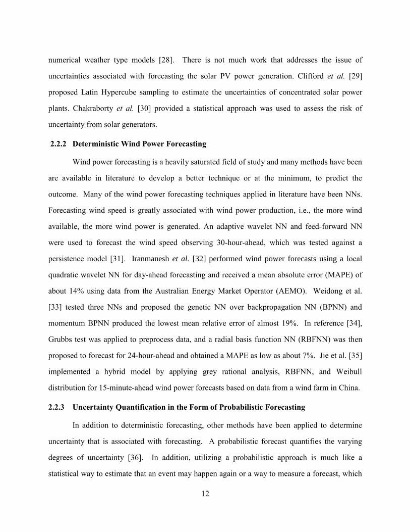
Figure 3.1 displays the functionality of how the PV power data is processed with WT

where the left side comprises of the decomposition phase and the right side consists of the

reconstruction phase. In Figure 3.1, the letter S represents the input signal of the true power that

was generated from the PV system, i.e. the historical actual power data. The true power put into

the signal is directly related to time. Moreover, the WT tool processes the actual power with

18

respect to a certain time of the day. The amount of time that is processed into the WT tool is

determined by the chosen forecast horizon, which varies by the day and season selected to

forecast. That signal is decomposed into low and high filtered frequencies, which is denoted as

L and H. Four decomposed signals are produced into three high frequencies (D1, D2, and D3)

that are detailed signals and a low frequency (A3) that is an approximation signal. In addition,

the signal reconstructs and are then represented with accent hats. For this thesis, a built-in house

code in MATLAB has been utilized for one-dimensional Daubechies wavelets. The number of

dimensions is the number of vanishing moments assisting in leveling out the data, thus

mitigating the fluctuations.

Figure 3.1: Wavelet decomposition and reconstruction process.

3.3 SOFT COMPUTING MODELS

NNs have been commonly utilized in forecasting applications and are based on the

anatomy of a brain. Artificial NNs are machine learning tools and are perceived as artificial

intelligence [51]. They are SCMs that have the basic structural design that is made up of neurons

within the input layer, hidden layer, and output layer where the hidden layer consists of transfer

functions where most technical commutations take place. The NNs are beneficial methods that

19

are used to learn and distinguish patterns by simulating similar behavior according to what was

learned [52]. In a NN, input data is separated for training and testing, detail of which is

discussed in Chapters 4 and 5. A lag time was applied, i.e., the past observation periods, which

varied according to the month and season as well as the forecasting horizons and forecast

intervals, see Appendix I. The input data is determined by the user, which is what the user

identifies as significantly correlated data to the application. In this thesis, solar irradiance (R),

temperature (T), and the true power output (PV) of the solar PV system are used as inputs. There

are various types of NNs, which are different, yet somewhat similar architecture. For example,

Figure 3.2 presents an example of the basic NN architecture.

Figure 3.2: A general architecture of a neural network.

This thesis utilized three types of SCMs that are BPNN, GRNN, and RBFNN.

Additionally, the architecture of BPNN, GRNN, and RBFNN is also presented in Figure 3.2.

The BPNN model is a frequently used NN, which utilizes the steepest descent method to find the

best solution [53]. BPNN applied in this work is a feed-forward network that that utilized the

transfer function tansig in the first part of hidden layer and purelin in the second half of the

hidden layer (summation layer). The architecture of RBFNN comprises of two layers, the first

and second in the hidden layer consists of a radial basis transfer function and a linear transfer

function, respectively [54] and similarly does the GRNN model [55]. However, they compute

20

slightly differently where GRNN performs with a normalized dot product in the summation layer

and RBFNN perform summations with a net product operator [54, 55]. The GRNN model can

handle non-linear applications [19]. Similarly, RBFNN is much faster than other NNs and has

the ability to approximate well [56]. Subsequently, BPNN, GRNN, and RBFNN are all able to

handle non-linear applications and complex problems. In Appendix I, Table AI.1 presents the

detailed specifications regarding amount of neurons and other NN parameters applied in this

study. In addition to Appendix I, Table AI.2 and Table AI.3 present the lag times applied in this

thesis and forecasting horizons. The NNs applied in this thesis did not use the application that

MATLAB provides, which is the user friendly input output interface. However, the NNs were

fully written in the built-in-house MATLAB code and are extensive. In Appendix II, an example

of the partial code of BPNN model is also provided.

3.4 OPTIMIZATION TECHNIQUES IN FORECASTING

There are many optimization techniques that have been applied in forecasting

applications. For example, a deterministic forecast was conducted using WT and a fuzzy

ARTMAP, which was optimized by a firefly method [12]. Another method applied in

forecasting was a support vector regression model that was improved with chaotic ant swarm

optimization [57]. There are various optimization techniques applied to forecasting such as

simulated annealing or firefly algorithm. In this study, GA and PSO are applied to optimize the

weights, bias, and spread of SCMs, i.e. BPNN, RBFNN, and GRNN, in order to enhance the

performances of these SCMs for better forecasting accuracy.

3.4.1 Genetic Algorithm

GA is an optimization technique that is used to find the most optimal solution in a

solution space. GA is based on the natural selection and evolution that has features such as

considering a population that has chromosomes that evolve from mutation or crossover [58]. In

this thesis, BPNN method is optimized by GA through the weights and biases, whereas the

spread of the weighted inputs are optimized in the GRNN and RBFNN method to minimize

21

error. Also, it is utilized as a supplementary method to find an ideal solution. The procedure of

the GA algorithm is illustrated in Figure 3.3.

In this study, the GA algorithm was coded in MATLAB. The algorithm begins with an

initial population and randomness during initialization of the mutation and crossover. Due to

random initialization, results varied with each simulation. In order to make the simulations

repeatable, the random variables were seeded to regenerate the same results. This way of

controlling the random variables could be easily removed since it was encoded for testing

purposes. The input parameters coded into the GA algorithm is presented in Appendix I, Table

AI.4.

Figure 3.3: GA process model.

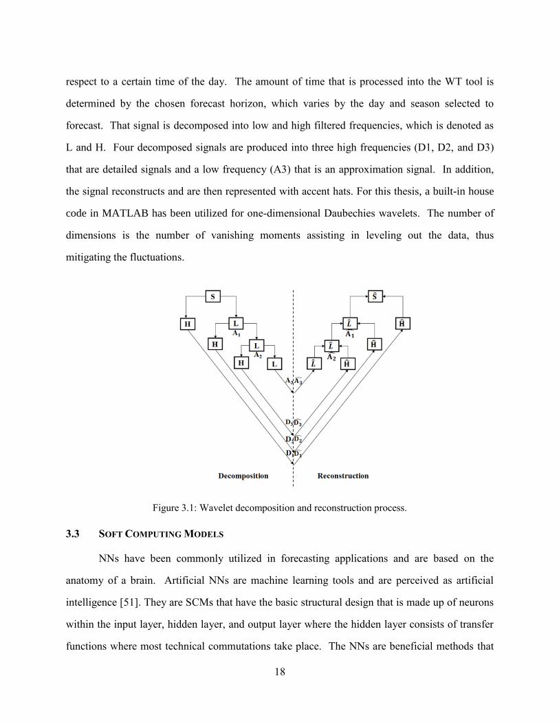
3.4.2 Particle Swarm Optimization

PSO is another optimization technique that searches the solution space to find the most

optimal solution, principally the ideal position at a particular velocity [59]. This method is most

commonly known to mimic the flight pattern to a flock of birds. As the birds fly through air

currents, they tend to move with one another at certain speeds finding the most ideal route in the

22

sky. In this thesis, BPNN method is optimized by PSO through the weights and biases, whereas

the spread of the weighted inputs are optimized in the GRNN and RBFNN method to decrease

error. The structure of PSO algorithm is shown in Figure 3.4.

In this study, the PSO algorithm was also applied as a function in MATLAB. The

algorithm begins with an initial amount of particles and initialization began with a random

position and velocities. Due to random initialization, results varied with each simulation. In

order to make the simulations repeatable, the random variables were seeded to regenerate the

same results. This way of controlling the random variables could be easily removed since it was

encoded for testing purposes. The PSO algorithm was coded in MATLAB and the input

parameters used for the PSO algorithm is presented in Appendix I, Table AI.5.

Figure 3.4: PSO algorithm process model.

23

3.5 PROBABILISTIC MODELS

Though there are various ways to estimate uncertainty. In this study, the output from the

deterministic solar PV power forecasts is used to estimate uncertainty using two methods: (i)

central limit theorem, and (ii) bootstrap method, which produces the confidence intervals. The

output of the deterministic forecast is considered a sample and is applied to the fundamental

approach known as the central limit theorem to form confidence intervals. These uncertainty

methods begin by defining a sample size. In this thesis, the sample size is defined by the number

of hours in the forecast horizon chosen. This is conducted through a parametric approach where

the variance is known based on a formula adopted from reference [60] and is presented below.

Z = –

(1)

P [ Mn(Y) – c ≤ μ ≤ Mn(Y) + c ] = 1- α (2)

Mn(Y) –

√ ≤ μ ≤ Mn(Y) +

√ (3)

Equation (1) is the margin of error, represented as Z, in which the equation within (1- α)

is the confidence coefficient and α is the confidence level. Equation (2) is the probability P of an

inequality where the whole term Mn(Y) denotes the sample mean, μ is the number in interest or

basis, n is the number of samples, and c is the standard error. Similarly in equation (3), σ is the

standard deviation from which was derived from the variance. From these equations, an upper

and lower bound can be determined to create confidence intervals.

Another technique to conduct uncertainty estimation that can be quantified from the

deterministic forecast by resampling through a method called bootstrap [61]. Uncertainty

quantification can be best represented in the form of probabilistic forecasts [12]. The importance

of applying a probabilistic forecast is to quantify the reliability of a specific method and interpret

the variations of an output [62]. Additionally, the bootstrap method is a useful inferential

process tool and assists in conclusive decision making [63]. The bootstrap method is based on

the central limit theorem, and the sample size is determined by the number of hours in the chosen

24

forecast horizon, yet applying the results from the hybrid intelligent models. The bootstrap

method applies the application of equations (1)-(3), but the standard error changes through

sampling. The confidence percentage can be determined by using equation (4) as presented

below.

Confidence level = (1 – α) * 100% (4)

An example of how the method works is to consider a large population from a jar that

contains various types of coins. Then take one coin out, that is chosen randomly, and record the

coin value, then put it back in the jar. Repeat this process where the coin is taken out and the

coin values are recorded, and then it is put back in the jar for a total of five times creating a

sample. Subsequently, resample as many times as desired creating subsets of five.

Bootstrapping can be computationally intensive, and therefore, was implemented in MATLAB.

The input data applied to a function in MATLAB to determine the confidence intervals are

forecasted results and α. MATLAB has provided a function for calculating bootstrap confidence

intervals, so no actual coded formulas are applied when finding the confidence intervals.

Obtaining a confidence interval will determine an upper and lower bound from the reference

deterministic forecast. This will provide a range of uncertainty that is associated with the

forecasts. Therefore, the uncertainty can be statistically measured and visualization can be

provided to determine that uncertainty.

3.6 SUMMARY

Chapter 3 provided information in the forecasting models applied in this thesis. The WT

technique functionality was explained and how it was applied to the data as a preprocessing tool.

The SCMs utilized to conduct the forecast were discussed providing the NN architecture. More

detail on how SCMs were enhanced through optimization algorithms was provided. The uses of

abbreviations are utilized throughout this thesis and a list of all these abbreviations can be found

in Appendix III. Finally, uncertainty quantification was described utilizing two uncertainty

methods, (i) central limit theorem and (ii) bootstrap confidence intervals. All models applied in

25

this thesis were fully coded in MATLAB except for bootstrap confidence intervals that used the

built-in-house function. In addition, the PC technical specifications and details that were used to

conduct the simulations are presented in Appendix IV.

26

Chapter 4: Applying Wavelets to Predict the Solar PV Power Output Using

Generalized Regression Neural Network

4.1 INTRODUCTION

In previous chapters, the motivation of this study, a detailed literature review of solar PV

power forecasting, a description of different forecasting models and uncertainty quantification

methods were all presented. This chapter focuses on short-term forecasting of the power

generation of a PV system. This chapter presents one scenario with prediction results for 1-hour-

ahead solar PV power forecasting, which the forecasting interval is also known as the forecasting

frequency. The forecasting is performed using individual SCMs (GRNN and RBFNN) and

hybrid intelligent models (WT+GRNN and WT+RBFNN). This scenario compares deterministic

intelligent models and proposes a hybrid intelligent model, WT+GRNN. The exceptional

qualities of the intelligent models, RBFNN and GRNN are the selected NNs in this study. In

addition, adding WT to GRNN builds a stronger combination. The inclusion of WT is necessary

and is best exemplified by reference [64]. The forecasting results obtained from the different

models are compared to assess the prediction capability of the proposed hybrid WT+GRNN

intelligent model.

4.2 INPUT DATA

For fair comparison, all the models were tested using the same data set acquired from a

15kW PV system located in Ashland, Oregon [10]. The data sets include hourly PV power

output in kW, global solar irradiance in Wh/m2 and temperature in degree Celsius. It is well

known that the most important parameter for solar PV power prediction is R [65]. In this study,

the correlation coefficient between the PV power output and R is found to be 0.97. Another

weather parameter such as wind speed was not as influential in the performance of the

forecasting algorithm and is not considered in this paper. The forecasting model output is for a

PV power forecast interval of 1-hour-ahead. For chapter 4, the forecast horizon is 12 hours,

which is the prediction period. Forecasting was carried out considering multiple seasons of the

year 2011.

27

4.3 PROPOSED HYBRID INTELLIGENT FORECASTING FRAMEWORK

The procedure to forecast the power generation of a PV system is based on input and

output process. A schematic diagram of the proposed hybrid WT+GRNN intelligent forecasting

model is shown in Figure 4.1. This process is similar to WT+RBFNN where the only difference

is replacing GRNN with RBFNN. The deterministic PV power forecasting procedure is

explained in the following steps:

Figure 4.1: Proposed deterministic hybrid WT+GRNN intelligent model for STPVF.

Step 1: Input and Decomposition

Nine input parameters of the proposed hybrid model are considered as solar radiation (Rt,

Rt-12, and Rt-20), temperature (Tt, Tt-12, and Tt- 20), and actual PV power output (PVt, PVt-12, and

PVt-20) where t is current hour. These inputs are decomposed into four components by WT. The

28

decomposed signals are: one low frequency (A3) and three high frequency (D1, D2, D3)

components.

Step 2: Process Inputs

Individual decomposed PV power signals (A3, D1, D2, D3) from step-1 along with solar

irradiance (R) and temperature (T) are then fed into the GRNN model. The GRNN model splits

up the data for approximately 30% of the data for testing and 70% for training. The past 15 days

before the forecast day are utilized for training of all the NNs used in chapter 4.

Step 3: Output

The output components of the GRNN model, i.e., forecasted decomposed low frequency

component ( ) and the forecasted high frequency signals ( , , and ) will undergo WT

reconstruction process and produce the desired hourly solar PV power forecasts.

4.4 RESULTS AND DISCUSSION

As mentioned earlier, this study presents STPVF using intelligent models. The

forecasting performances of the intelligent models are compared using RBFNN, GRNN,

WT+RBFNN and WT+GRNN. In this scenario, WT+GRNN is the best performing hybrid

intelligent model that is determined by the best accuracy and the lowest errors.

4.4.1 Forecasting Accuracy Measures

The forecasting accuracy of the forecasting models are assessed by using three accuracy

measures, MAPE, mean absolute error (MAE), and RMSE.

MAPE =

∑

|

|

* 100% (5)

MAE =

∑ |

|

* 100% (6)

RMSE = √

∑ (

)

* 100% (7)

29

Where N is the total number of data points, is the forecasted power data,

is the actual

power data, and is the average of the actual power. The significance of taking the average

of the actual power is that the actual value is small and subsequently will cause a large MAPE

even if the differences between the forecasted and actual values are small.

4.4.2 One-Hour-Ahead Forecasting Results

Forecasting the power output for a PV system using SCMs is carried out in all four

seasons. From each season, two different days (Day1 and Day2) were chosen randomly.

Utilizing the MAPE definition as described in (5), Table 4.1 presents the results obtained from

the hybrid WT+GRNN model, and the results are compared with other SCMs such as RBFNN,

GRNN, and WT+RBFNN. As it can be observed from Table 4.1 for winter Day1, the MAPE

obtained from the RBFNN model is 16.73%, whereas with the GRNN, it is 13.73%. These errors

are among the highest. A possibility to the higher forecasting error could be the cause of

different reasons such as cold day on Day1 or it could have been cloudy, or maybe a combination

of them. However, when WT is combined with these models, an improvement of about 26% and

56% in MAPEs was observed from the WT+RBFNN and WT+GRNN (proposed), respectively.

It can also be observed in winter (Day2) that the improvement in forecasting error by the

proposed WT+GRNN as well as WT+RBFNN models is comparatively better than that of Day1.

Almost a similar trend can be seen in Table 4.1 where RBFNN possesses the highest MAPE and

GRNN model performing better than WT+RBFNN in most simulated cases; particularly in fall

(Day2), the MAPE obtained from GRNN (3.67%) is about 68% lower than that of WT+RBFNN

(11.39%). These observations depict that the forecasting performances of the considered SCMs

with or without WT are seasonal sensitive and their forecasting performances are inconsistent.

However, in all the simulated cases, the MAPEs obtained from the proposed hybrid WT+GRNN

model are lower than or around 5% in all the seasons except in spring (Day2). For all seasons,

the MAPEs obtained from the RBFNN model are in the range of 2.93% to 16.73%, whereas it is

1.68% to 13.73% for GRNN, 1.78% to 12.28% for WT+RBFNN, and 1.59% to 10.56% for the

30

Table 4.1: Comparison of forecasting performance of the proposed hybrid WT+GRNN intelligent model

with other models.

Model Error Winter Spring Summer Fall

Day1 Day2 Day1 Day2 Day1 Day2 Day1 Day2

RBFNN

MAPE 16.73 10.00 3.46 14.10 2.93 5.22 7.54 14.44

MAE 0.81 0.41 0.29 1.12 0.21 0.43 0.40 0.94

RMSE 1.05 0.54 0.41 1.25 0.27 0.53 0.50 1.31

GRNN

MAPE 13.73 6.29 1.68 12.75 2.27 3.62 5.83 3.67

MAE 0.66 0.26 0.14 1.01 0.16 0.30 0.31 0.23

RMSE 1.06 0.37 0.19 1.26 0.20 0.36 0.41 0.29

WT+RBFNN

MAPE 12.28 8.93 1.78 12.84 2.82 4.15 7.38 11.39

MAE 0.59 0.36 0.15 1.02 0.20 0.34 0.39 0.74

RMSE 0.72 0.43 0.17 1.18 0.26 0.40 0.47 1.08

WT+GRNN

(proposed)

MAPE 6.02 5.21 1.59 10.56 1.94 3.11 5.65 2.90

MAE 0.29 0.21 0.13 0.84 0.14 0.25 0.30 0.18

RMSE 0.40 0.40 0.32 0.18 1.06 0.32 0.40 0.24 Note: MAPE in %, MAE and RMSE in kW

proposed WT+GRNN model. This demonstrates the effectiveness of using WT. The forecasting

performances of these models are further compared by calculating MAE and RMSE as shown in

Table 4.1 where we can observe the lower values of these accuracy measures by the proposed

WT+GRNN model.

Figure 4.2: MAPE histogram comparing performances of the SCMs and hybrid models.

31

Additionally, Figure 4.2 presents Day1 for all seasons, which can be observed that

WT+GRNN is represented by the purple cone holding the lowest errors. Note that in all the

simulated cases, the test results demonstrate the superior predicting performance of WT+GRNN

model over the tested alternatives.

4.5 SUMMARY

Chapter 4 presented several deterministic approaches to forecast solar PV power

generation. The focus of chapter 4 provided a proposal by combining WT with a SCM based on

GRNN. It began with a brief background and presented the input data applied in chapter 4, which

was PV, R, and T. Then, the forecasting framework of WT+GRNN was presented and the

results were discussed. By applying the accuracy measures as described earlier, the deterministic

forecasted results1 demonstrated that the hybrid intelligent WT+GRNN model was the superior

model.

1 Findings of this chapter are communicated in IEEE co-sponsored conference as indicated below:

P. Mandal, A. U. Haque, S. T. S. Madhira and D. I. Al-Hakeem, “Applying wavelets to predict solar PV

output power using generalized neural network,” in Proc. North American Power Symposium (NAPS),

2013.

32

Chapter 5: Uncertainties Quantification of Solar PV Power Forecasts Using

Bootstrap Confidence Intervals

5.1 INTRODUCTION

In the previous chapter 4, a deterministic approach was applied to STPVF without using

any uncertainty estimation or optimization methods and forecasting results were presented for 1-

hour-ahead solar PV power forecasting. Chapter 5 provides another case of a more detailed

deterministic approach that utilizes more SCMs and hybrid intelligent models. Chapter 5 also

presents the application of optimization algorithms, mainly PSO and GA, in order to enhance the

forecasting performance of the SCMs. The deterministic forecasting obtained in this chapter

will then be followed by the uncertainty estimation of the deterministic forecasts using central

limit theorem and bootstrap methods. The following presents the procedure of the proposed

forecasting method then discusses results from the forecast and uncertainty estimation of the

solar PV generation from the PV system.

There are two major scenarios performed for deterministic forecasting in chapter 5.

Scenario-1: Solar PV power forecasting results for two random days in each season for

various forecasting horizons.

Scenario-2: Solar PV power forecasting results for a sunny day (SD), cloudy day (CD),

and a rainy day (RD) for various forecasting horizons.

STPVF was carried out using several SCMs, and then compared with the proposed hybrid

WT+RBFNN+PSO intelligent model. All of the SCMs models and the proposed model utilized

the MATLAB software to perform complex computations involving artificial NNs, optimization,

and uncertainty estimation in order to conduct the forecasts. An example of the BPNN code

utilized in this study can be seen in Appendix II.

5.2 INPUT DATA

For an unbiased comparison was created using the same set of test data that was collected

from a 15 kW PV system in Ashland, Oregon [10]. The hourly data applied in this work,

beginning with the most important data, was the actual PV power output (kW), global solar

33

irradiance (Wh/m2) and temperature (°C). To provide more scenarios, the forecasting hours used

to conduct tests had varied forecasting intervals for 1-hour-ahead, 3-hour-ahead, and 6-hour-head

forecasting. The forecasting horizons utilized in chapter 5 also varied from 7 to 12 hours, which

is also known as the forecasting period. The variations in the forecasting horizons are due to

daylight availability where there is more light in the summer and least amount of light in the

winter. In the summer time, the forecasting horizon was 12 hours since the daylight lasted

longer during this time. In the fall, the forecasting horizon varied between 8 and 11 hours since

there was a transition from longer daylight to less daylight. In the winter, the forecasting horizon

varied between 8 and 9 hours, which had the least amount of daylight. In the spring, the

forecasting horizon varied between 11 and 12 hours since there was a transition from less

daylight to more daylight. For the forecast horizon time that correlates with Tables 5.1-5.4, see

Appendix I, Table AI.1. The preceding times of observations, known as the lag time, is another

parameter that was adjusted according to time of power production that began from the

previously observed period. This too was affected by seasonality and daylight limitations. This

study utilized three lag times to account for the daylight differences. For the Tables 5.2-5.4

corresponding lag times, see Appendix I, Table AI.2.

5.3. PROPOSED HYBRID INTELLIGENT FORECASTING FRAMEWORK

The proposed hybrid intelligent model is a combination of WT that is a data filtering

technique and a SCM based on RBFNN. The short-term solar PV power generation forecasting

process using the proposed hybrid WT+RBFNN+PSO is depicted in Figure 5.1.

34

Figure 5.1: Schematic diagram of the proposed hybrid WT+RBFNN+PSO intelligent model.

The step-by-step forecasting procedure is described below.

Step 1: Input

Nine inputs are considered for the proposed approach by initialization that is T, R, and

PV, which are time-series data. The associated lag time for each input are shown in Appendix I.

Then, decomposition follows where only one input is subjected to the WT and then decomposed,

which is the actual power generation. The decomposition phase splits the data into the low

frequency (A3) and high frequency signals (D1, D2, D3).

Step 2: NN optimization

After each decomposed signal developed, actual PV power (A3, D1, D2, and D3) were

then inserted to the RBFNN method that was optimized through PSO. The RBFNN model splits

up the data for approximately 30% of the data for testing and 70% for training. The past 15 days

before the forecast day are utilized for training of all the NNs used in chapter 5.

35

Step 3: WT Reconstruction

When the training was completed, each of the PV power signals ( , , and ) were

reconstructed individually utilizing WT while forecasting to produce a prediction of the PV

power with respect to time by the hour.

Step 4: Confidence Intervals

Once the deterministic forecast is established, the forecasted output is used as a basis for

the uncertainty estimation. That output information from the forecast is then applied to bootstrap

method where it is resampled to develop confidence intervals at various confidence percentages,

which ranged from 10%-95% for testing purposes.

5.4 SIMULATION RESULTS AND DISCUSSION

The following presents the results of the solar PV power generation forecast from the PV

system and discusses the results from the forecast. First, the forecasting accuracy measures that

are utilized in chapter 5 are presented. Then, the forecasted results are provided for 1-hour-

ahead, 3-hour-ahead, and 6-hour-ahead. Moreover, different day types are forecasted that are

further analyzed using SDs, CDs, and RDs. Finally, uncertainty estimation is quantified using

the results from the deterministic forecast. To generate different scenarios, all techniques were

tested in each season, i.e. spring, summer, fall, and winter.

5.4.1 Forecasting Accuracy Measures

To determine the amount of accuracy that each model projected, different types of ways

to determine error were used and are shown in equations (5), (8), and (9). Equations (8)-(10) are

normalized root mean square error (NRMSE), normalized mean absolute error (NMAE), and

variance (σ2). Within these following equations are N, which is the number of data points,

is the actual solar PV power, and is the forecasted PV power. The capacity of the solar PV

system used is 15 kW that is denoted and the average of the actual power is signified as

.

36

NMSE = √

∑ (

)

x 100% (8)

NMAE =

∑

x 100% (9)

σ2 =

∑ (

|

|

∑

|

|

)

(10)

5.4.2 Solar PV Power Forecasting Results for Various Forecasting Horizons

The following presents an evaluation of the results generated from several deterministic

SCMs, hybrid models, and the proposed model for comparison. In order to test the methods,

different scenarios were applied such as using two random days within each season which are

represented in Tables 5.1-5.4 as D1 for day 1 and D2 for day 2. Table 5.1 presents the dates that

were randomly selected for forecasting and are the same dates used for Tables 5.1-5.3, which

presents the solar PV power forecasting performance of several models using equations (5), (8),

and (9) to provide different accuracy measurements. Since there are plenty of results, D1 of

spring will be used for comparison as an example of the forecasting performance for the sections

under sub-section (5.4.2).

Table 5.1: Randomly chosen forecasting days.

Winter Fall Summer Spring

Day 1 (D1) 12/23/2011 09/22/2011 07/10/2011 05/21/2011

Day 2 (D2) 02/03/2011 11/02/2011 06/14/2011 05/03/2011

5.4.2.1 One-Hour-Ahead Solar PV Power Forecasting Results

Table 5.2 compares 12 models forecasted at 1-hour-ahead. In Table 5.2, BPNN is

presented with three accuracy measures, and then hybridized with WT that is also presented with

3 accuracy measures. Then, WT+BPNN was further combined with GA and separately with

PSO in order to optimize the weights and bias parameters of BPNN to enhance its performance.

This hybridization method is also carried out with GRNN and RBFNN. In D1 of spring, the

37

Table 5.2: One-hour-ahead forecasting performance of WT+ RBFNN+PSO model with other models.

Forecasting

Model

Accuracy

Measures

Winter Fall Summer Spring

D1 D2 D1 D2 D1 D2 D1 D2

BPNN

NMAE 10.66 7.04 4.14 3.25 11.14 6.17 6.12 5.65

NRMSE 13.50 10.11 5.32 4.16 13.44 8.66 7.57 7.98

MAPE 30.82 16.33 9.01 6.20 19.53 10.24 10.34 8.67

WT+BPNN

NMAE 7.94 5.14 7.72 8.85 7.97 5.96 7.48 5.84

NRMSE 10.19 5.94 10.24 10.24 9.74 7.32 11.21 6.41

MAPE 22.95 11.93 16.82 16.88 13.96 9.89 13.11 8.96

WT+

BPNN+GA

NMAE 3.20 23.12 5.44 7.57 8.52 22.74 18.67 11.48

NRMSE 4.70 26.65 7.38 8.84 14.20 25.76 21.94 12.81

MAPE 9.26 53.67 11.85 14.44 14.93 37.76 31.56 17.62

WT+

BPNN+PSO

NMAE 9.70 3.73 4.75 3.29 9.35 5.21 11.18 9.79

NRMSE 10.77 4.91 5.55 4.84 16.10 6.69 13.18 11.21

MAPE 28.06 8.66 10.35 6.27 16.38 8.65 18.90 15.02

GRNN

NMAE 7.44 3.52 2.31 2.45 2.21 3.61 9.07 8.84

NRMSE 9.53 4.45 3.95 3.15 3.54 5.88 15.10 11.90

MAPE 21.51 7.30 5.04 4.67 3.87 5.99 15.33 13.56

WT+GRNN

NMAE 5.05 2.18 2.12 2.40 2.06 3.21 5.99 7.15

NRMSE 5.84 2.81 3.73 3.19 3.37 4.82 8.09 9.20

MAPE 14.62 5.07 4.63 4.57 3.61 5.34 10.12 10.96

WT+

GRNN+GA

NMAE 4.86 2.13 4.77 2.59 2.04 3.43 6.48 6.60

NRMSE 5.82 3.03 6.41 3.52 3.24 5.39 8.65 8.35

MAPE 14.05 4.96 12.42 4.93 3.59 5.70 10.96 10.13

WT+

GRNN+PSO

NMAE 4.98 2.07 2.08 2.28 1.96 2.91 5.43 6.64

NRMSE 5.61 2.80 3.59 2.71 3.19 4.11 7.43 8.64

MAPE 14.41 4.82 4.53 4.35 3.44 4.84 9.18 10.18

RBFNN

NMAE 10.74 4.67 2.48 3.94 4.04 5.23 9.63 8.06

NRMSE 15.46 8.03 3.21 4.42 4.59 7.70 12.00 10.77

MAPE 31.06 10.84 5.39 7.52 7.08 8.68 16.28 12.37

WT+RBFNN

NMAE 4.21 2.19 2.09 4.33 3.20 5.45 10.83 6.57

NRMSE 5.65 3.16 2.63 6.06 4.07 7.28 12.64 8.07

MAPE 12.18 5.09 4.58 8.27 5.60 9.06 18.31 10.09

WT+

RBFNN+GA

NMAE 3.88 2.20 2.72 2.22 2.06 2.32 3.60 4.64

NRMSE 4.87 2.96 3.11 3.34 2.67 3.50 5.15 7.62

MAPE 11.23 5.12 5.92 4.23 3.62 3.86 6.08 7.12

WT+

RBFNN+PSO

(proposed)

NMAE 3.32 1.92 2.06 1.42 2.46 2.12 3.58 6.55

NRMSE 3.91 2.55 2.57 1.85 2.72 2.48 4.84 10.98

MAPE 9.60 4.45 4.51 2.70 4.30 3.51 6.06 10.05

38

BPNN model acquired a NMAE of 6.12%, WT+BPNN performed with an error of 7.48%,

WT+BPNN+GA at 18.67%, and WT+BPNN+GA acquired 11.18%. BPNN performed the best,

yet performed the least best by hybridizing the method. Also during D1 of spring, GRNN

obtained a NMAE of 9.07%, WT+GRNN performed with an error of 5.99%, WT+GRNN+GA at

6.48%, and WT+GRNN+PSO acquired 5.43%. In this case, WT+GRNN+PSO acquired the least

amount of error. In addition, RBFNN obtained a NMAE of 9.63%, WT+RBFNN acquired

10.83%, WT+RBFNN+GA at 3.60%, and WT+RBFNN+PSO achieved 3.58%. So far,

WT+RBFNN+PSO performed the best out of all the methods in spring D1. Although this is a

comparison of one of the days in spring, WT+RBFNN+PSO obtained the lowest error in most

tested cases. In Table 5.2, the top 3 best performing models were WT+GRNN+PSO,

WT+RBFNN+GA, and WT+RBFNN+PSO. The NMAE range for WT+GRNN+PSO is

approximately 2% to 6.6%, WT+RBFNN+GA ranged from about 2% to 4.6%, whereas the

proposed method, WT+RBFNN+PSO, ranged at approximately 1.4% to 6.5%. The results

indicate that each day and different season produce different errors and the forecast can be daily

sensitive within each season.

Figure 5.2: Comparison of the actual power generation and forecasted solar PV power using

WT+RBFNN+PSO.

39

Figure 5.3: Comparison of the forecasting performance of the proposed WT+RBFNN+PSO model with

WT+GRNN+PSO.

Figures 5.2 and 5.3 was generated to provide a visual of the forecasts compared to how

close they were to the actual solar PV power used from the historical data for 1-hour-ahead. In

Figure 5.2, the red line indicates the historical actual PV power from the solar PV system and the

blue line indicates the forecasted values of WT+RBFNN+PSO on December 23, 2011. The

forecasted date associated with Figure 5.2 can be found in Table 5.1 (December 23, 2011). In

Figure 5.3, the red line indicates the historical actual PV power from the solar PV system, the

blue line indicates the forecasted values of WT+GRNN+PSO and additionally, a green line

which indicates the forecasted values of WT+RBFNN+PSO. The forecasted date associated with

Figure 5.3 can be found in Table 5.1 (May 21, 2011).

5.4.2.2 Three-Hour-Ahead Solar PV Power Forecasting Results

Since there are plenty of results, D1 of spring will be used for comparison as an example

of the forecasting performance for this sub-section (5.4.3). Table 5.3 compares six models

forecasted for 3-hour-ahead forecasts. These models are amongst the best performing models

from Table 5.2 and as for a fair further comparison, spring D1 will be analyzed. In

spring D1, WT+GRNN attained a NMAE of 16.4%, WT+GRNN+GA acquired 16.91%, and

40

Table 5.3: Three-hour-ahead forecasting performance of the proposed model with other models.

Forecasting

Model

Accuracy

Measures

Winter Fall Summer Spring

D1 D2 D1 D2 D1 D2 D1 D2

WT+GRNN

NMAE 9.74 7.17 2.57 7.08 1.89 3.88 16.40 7.63

NRMSE 23.37 9.56 4.00 9.10 2.97 6.29 21.20 12.65

MAPE 28.18 16.65 5.61 13.50 3.31 6.44 27.72 11.70

WT+

GRNN+GA

NMAE 8.51 11.15 6.75 7.04 1.65 4.05 16.91 8.50

NRMSE 11.26 17.43 10.84 8.98 2.68 6.49 21.89 14.57

MAPE 24.62 25.89 17.57 13.43 2.88 6.72 28.59 13.03

WT+

GRNN+PSO

NMAE 9.50 7.78 2.44 4.92 1.84 3.16 15.77 7.26

NRMSE 12.24 9.88 3.83 5.85 2.74 4.98 20.76 10.39

MAPE 27.47 18.07 5.33 9.38 3.24 5.25 26.66 11.14

WT+RBFNN

NMAE 9.86 3.75 3.52 9.99 3.61 6.51 15.49 11.27

NRMSE 13.04 5.25 4.15 14.05 4.48 9.31 29.33 13.99

MAPE 28.50 8.71 7.67 19.05 6.33 10.81 26.18 17.29

WT+

RBFNN+GA

NMAE 5.29 4.19 3.79 3.37 2.15 4.84 10.29 11.86

NRMSE 6.56 5.90 5.29 4.53 3.08 6.25 12.95 16.35

MAPE 15.30 9.72 8.25 6.42 3.76 8.03 17.40 18.19

WT+

RBFNN+PSO

(Proposed)

NMAE 6.21 4.13 3.21 4.24 3.10 4.72 9.27 13.68

NRMSE 8.00 4.95 4.38 5.29 3.81 6.14 11.24 17.84

MAPE 17.97 9.60 6.99 8.09 5.43 7.84 15.67 20.98

WT+GRNN+PSO obtained 15.77%. WT+GRNN+PSO achieved the best performance with

lowest NMAE’s compared to the other GRNN models. Additionally, WT+RBFNN attained a

NMAE of 15.49%, WT+RBFNN+GA acquired 10.29%, and WT+RBFNN+PSO obtained

9.27%. So far, WT+RBFNN+PSO achieved the best performance with the lowest NMAE’s in

spring D1. However, WT+RBFNN+PSO and WT+RBFNN+GA performed very similar in this

the case based on their average and did not outperform one another.

5.4.2.3 Six-Hour-Ahead Solar PV Power Forecasting Results

Since there are plenty of results, D1 of spring will be used for comparison as an example

of the forecasting performance for this sub-section (5.4.4). Table 5.4 compares the same six

models as well, similar to Table 5.3, only forecasting for 6-hour-ahead. In D1 of spring,

WT+GRNN attained a NMAE of 24.12%, WT+GRNN+GA acquired 24.67%, and

41

Table 5.4: Six-hour-ahead forecasting performance of the proposed model with other models.

Forecasting

Model

Accuracy

Measures

Winter Fall Summer Spring

D1 D2 D1 D2 D1 D2 D1 D2

WT+GRNN

NMAE 9.48 9.43 3.83 13.06 1.71 4.10 24.12 14.84

NRMSE 10.14 12.83 4.87 16.27 2.98 6.39 31.53 19.29

MAPE 27.42 21.89 8.34 24.90 2.99 6.82 40.77 22.77

WT+

GRNN+GA

NMAE 11.64 9.40 8.27 13.58 2.15 4.17 24.67 15.02

NRMSE 13.11 15.90 16.26 16.87 3.15 6.51 32.04 19.37

MAPE 33.67 21.81 21.52 25.88 3.76 6.92 41.70 23.04

WT+

GRNN+PSO

NMAE 9.60 10.32 3.53 6.84 2.08 3.16 24.90 14.90

NRMSE 10.30 13.05 4.61 8.09 3.14 5.02 31.54 18.27

MAPE 27.77 23.96 7.70 13.05 3.65 5.25 42.11 22.86

WT+RBFNN

NMAE 12.55 7.48 4.64 9.45 3.78 8.38 20.19 22.40

NRMSE 13.76 9.68 6.98 11.00 4.89 11.37 25.45 26.80

MAPE 36.29 17.38 10.10 18.02 6.28 13.92 34.14 34.36

WT+

RBFNN+GA

NMAE 8.50 10.49 3.54 6.08 2.12 8.64 19.06 14.90

NRMSE 9.68 12.56 5.18 7.04 2.82 10.31 21.98 17.72

MAPE 24.57 24.37 7.72 11.59 3.72 14.36 32.22 22.86

WT+

RBFNN+PSO

(Proposed)

NMAE 9.32 10.62 3.17 5.71 3.48 8.24 20.17 13.74

NRMSE 11.17 12.46 5.29 6.72 4.24 10.18 23.11 16.03

MAPE 26.98 24.65 6.91 10.89 6.10 13.69 34.09 21.07

WT+GRNN+PSO obtained 24.9%. WT+GRNN+PSO achieved the best performance with

lowest NMAE’s compared to the other GRNN models. Additionally, WT+RBFNN attained a

NMAE of 20.19%, WT+RBFNN+GA acquired 19.06%, and WT+RBFNN+PSO obtained

20.17%. In this case, WT+RBFNN+GA achieved the best performance with the lowest NMAE’s

in spring D1. Though, WT+RBFNN+GA and WT+RBFNN+PSO performed very similar in this

case and did not defeat each other.

5.4.3 Forecasting Results for Sunny Days, Cloudy Days, and Rainy Days

The following presents a different assessment of the results generated from four hybrid

models (WT+GRNN+GA, WT+GRNN+PSO, WT+RBFNN+GA, and WT+RBFNN+PSO)

including the proposed model for comparison, which are the models used in Table 5.2-5.4. In

order to further test the methods, different scenarios were applied by using 3 types of days within

each season that are represented in Table 5.5 and different lead ahead times which are indicated

42

in each Table’s caption. For the forecasting horizon times and lag times see Appendix I, Table

AI.3. Tables 5.6, 5.8, and 5.10 have the winter and fall seasons, whereas Tables 5.7, 5.9, and

5.11 have the summer and spring seasons. Table 5.5 presents the three days selected for

forecasting and are the same dates used for Table 5.6-5.11. In Table 5.6-5.11, these three days

are denoted SD, CD, and RD.

Table 5.5: Selected SDs, CDs, and RDs in different seasons.

Winter Fall Summer Spring

Sunny Day (SD) 02/12/2011 10/28/2011 07/28/2011 05/13/2011

Cloudy Day (CD) 02/11/2011 11/04/2011 07/12/2011 05/09/2011

Rainy Day (RD) 02/08/2011 10/07/2011 07/17/2011 05/31/2011

5.4.3.1 One -Hour-Ahead Forecasting Results for Sunny Days, Cloudy Days, and Rainy Days

Continuing forward with further analysis using spring, Table 5.7 presents the

performance for 1-hour-ahead forecasts. On SD WT+GRNN+GA obtained a NMAE of 9.13%,

CD’s NMAE was 10.55%, and 16.67% on RD. In contrast, WT+GRNN+PSO attained a lower

NMAE of 8.15%, CD’s NMAE was 9.86 however, it was 17.35% on RD making it higher than

Table 5.6: One-hour-ahead forecasting performance of hybrid models in winter and fall.

Forecasting

Model

Accuracy

Measures

Winter Fall

SD CD RD SD CD RD

WT+

GRNN+GA

NMAE 6.17 8.56 9.59 7.44 10.25 9.51

NRMSE 7.53 14.10 13.34 10.38 12.44 13.57

MAPE 12.14 25.84 57.03 21.80 42.30 37.23

WT+

GRNN+PSO

NMAE 5.98 8.55 7.75 6.09 8.68 9.05

NRMSE 7.37 14.19 10.81 9.38 11.76 12.67

MAPE 11.78 25.82 46.11 21.81 43.64 41.68

WT+

RBFNN+GA

NMAE 5.47 4.12 3.44 5.16 4.89 3.31

NRMSE 6.47 5.45 4.65 7.49 6.37 4.21

MAPE 10.76 12.43 20.46 18.47 24.59 15.26

WT+

RBFNN+PSO

(proposed)

NMAE 5.03 3.53 3.44 6.34 2.81 2.61

NRMSE 6.82 4.18 4.47 8.58 4.57 3.37

MAPE 9.89 10.67 20.46 22.69 14.13 12.01

43

that with GA. WT+RBFNN+GA on SD acquired a NMAE of 5.52%, CD attained 6.47%, and

8.06% on RD. WT+RBFNN+PSO succeeded the others by a NMAE of 4.42%, also 5.37% on

CD, yet not RD that was 9.95%. For 1-hour-ahead forecasts, the proposed model achieved the

lowest values compared to the other models in Table 5.7. As mentioned earlier, Table 5.6 has

the colder seasons and spring is being discussed as an example.

Table 5.7: One-hour-ahead forecasting performance of hybrid models in summer and spring.

Forecasting

Model

Accuracy

Measures

Summer Spring

SD CD RD SD CD RD

WT+

GRNN+GA

NMAE 0.67 19.15 13.18 9.13 10.55 16.67

NRMSE 0.78 26.34 16.61 13.44 13.75 20.40

MAPE 1.23 68.85 45.49 17.08 29.27 67.31

WT+

GRNN+PSO

NMAE 0.97 20.55 13.98 8.15 9.86 17.35

NRMSE 1.15 26.70 18.79 11.96 12.53 21.36

MAPE 1.79 73.86 48.22 15.25 27.35 70.05

WT+

RBFNN+GA

NMAE 1.23 6.44 6.28 5.52 6.47 8.06

NRMSE 1.82 7.76 7.73 5.98 8.58 10.65

MAPE 2.24 23.15 21.67 10.32 17.96 32.57

WT+

RBFNN+PSO

(proposed)

NMAE 1.13 5.65 8.31 4.42 5.37 9.95

NRMSE 1.67 7.22 10.87 5.18 7.23 12.77

MAPE 2.07 20.31 28.68 8.28 14.90 40.19

5.4.3.2 Three-Hour-Ahead Forecasting Results for Sunny Days, Cloudy Days, and Rainy Days

In Table 5.8 and 5.9, four models are compared for 3-hour-ahead. On SD of spring,

WT+GRNN+GA obtained a NMAE of 13.97%, CD’s NMAE was 15.25%, and 15.76% on RD.

In contrast, WT+GRNN+PSO attained a lower NMAE of 13.78%, CD’s NMAE was 13.51%

however, it was 17.17% on RD making it higher than that with GA. WT+RBFNN+GA on SD

acquired a NMAE of 7.54%, CD attained 10.12%, and 14.14% on RD. WT+RBFNN+PSO

succeeded the others by a NMAE of 4.96%, yet not 10.21% on CD, or RD that was 14.78%. For

3-hour-ahead, the proposed model did not achieve the lowest values compared to the other

models in Table 5.9.

44

Table 5.8: Three-hour-ahead forecasting performance of hybrid models in winter and fall.

Forecasting

Model

Accuracy

Measures

Winter Fall

SD CD RD SD CD RD

WT+

GRNN+GA

NMAE 11.13 6.52 9.91 12.10 18.17 12.76

NRMSE 14.05 7.78 11.60 15.30 20.95 17.63

MAPE 21.91 19.67 58.95 35.47 74.99 49.97

WT+

GRNN+PSO

NMAE 11.03 7.74 10.83 10.14 14.64 13.07

NRMSE 14.07 6.57 11.86 13.81 18.78 18.25

MAPE 21.72 19.82 64.43 36.32 73.59 60.25

WT+

RBFNN+GA

NMAE 8.16 7.49 7.93 9.58 6.89 5.93

NRMSE 10.88 8.94 9.81 12.95 8.41 7.80

MAPE 16.06 22.61 47.18 34.32 34.64 27.33

WT+

RBFNN+PSO

(proposed)

NMAE 11.55 8.26 10.63 9.99 8.21 7.65

NRMSE 13.28 9.52 11.96 12.87 10.07 9.43

MAPE 22.74 24.92 63.26 35.80 41.27 35.26

Table 5.9: Three-hour-ahead forecasting performance of hybrid models in summer and spring.

Forecasting

Model

Accuracy

Measures

Summer Spring

SD CD RD SD CD RD

WT+

GRNN+GA

NMAE 0.66 19.50 22.37 13.97 15.25 15.76

NRMSE 0.76 27.25 31.26 22.92 18.65 24.37

MAPE 1.22 70.09 77.18 26.11 42.31 63.63

WT+

GRNN+PSO

NMAE 1.02 19.14 22.37 13.78 13.51 17.17

NRMSE 1.22 27.56 31.26 21.27 16.79 25.27

MAPE 1.86 68.81 77.20 25.77 37.48 69.33

WT+

RBFNN+GA

NMAE 1.63 15.10 14.08 7.54 10.12 14.14

NRMSE 1.95 21.71 20.11 8.87 14.20 20.69

MAPE 2.99 54.28 48.58 14.11 28.09 57.11

WT+

RBFNN+PSO

(proposed)

NMAE 1.65 18.46 11.36 4.96 10.21 14.78

NRMSE 1.93 24.42 17.11 5.85 14.83 21.45

MAPE 3.02 66.36 39.22 9.29 28.34 59.70

45

5.4.3.3 Six-Hour-Ahead Forecasting Results for Sunny Days, Cloudy Days, and Rainy Days

Table 5.10: Six-hour-ahead forecasting performance of hybrid models in winter and fall.

Forecasting

Model

Accuracy

Measures

Winter Fall

SD CD RD SD CD RD

WT+GRNN+

GA

NMAE 20.11 15.75 13.68 11.21 11.19 10.39

NRMSE 22.11 19.57 18.77 13.76 15.21 15.10

MAPE 39.58 47.54 81.37 32.82 46.18 40.73

WT+GRNN+

PSO

NMAE 20.05 15.81 14.28 9.09 9.48 8.82

NRMSE 22.08 19.60 18.28 12.24 13.93 13.44

MAPE 39.47 47.71 84.94 32.57 47.69 40.64

WT+RBFNN+

GA

NMAE 14.12 8.73 21.71 11.11 9.85 7.39

NRMSE 15.97 12.89 26.15 14.12 12.54 8.59

MAPE 27.79 26.35 129.10 39.81 49.53 34.09

WT+RBFNN+

PSO

(proposed)

NMAE 16.41 11.37 20.51 10.95 8.23 7.91

NRMSE 18.96 15.05 25.91 13.88 9.42 9.50

MAPE 32.31 34.30 122.01 39.19 41.37 36.48

Table 5.11: Six-hour-ahead forecasting performance of hybrid models in summer and spring.

Forecasting

Model

Accuracy

Measures

Summer Spring

SD CD RD SD CD RD

WT+GRNN+

GA

NMAE 0.67 27.47 29.75 17.11 14.53 20.13

NRMSE 0.78 35.69 36.34 22.02 17.45 27.39

MAPE 1.23 98.75 102.63 32.01 40.30 81.29

WT+GRNN+

PSO

NMAE 1.00 28.19 29.84 17.22 14.03 19.04

NRMSE 1.21 36.37 36.44 22.04 16.73 26.15

MAPE 1.84 101.32 102.93 32.21 38.94 76.92

WT+RBFN+

GA

NMAE 2.03 27.69 24.85 9.26 9.74 23.87

NRMSE 2.50 35.07 31.94 11.05 14.04 28.54

MAPE 3.71 99.53 85.72 17.32 27.03 96.38

WT+RBFN+

PSO

(proposed)

NMAE 2.59 26.48 24.35 6.57 8.95 26.61

NRMSE 2.95 34.36 30.47 8.49 12.92 31.41

MAPE 4.75 95.18 84.00 12.29 24.85 107.47

Table 5.10 and 5.11 compares four models in the warmer seasons for 6-hour-ahead. On

SD of spring, WT+GRNN+GA obtained a NMAE of 17.11%, CD’s NMAE was 14.53%, and

20.13% on RD. In contrast, WT+GRNN+PSO attained a higher NMAE of 17.22%, however

CD’s and RD’s NMAE was lower than that with GA which was 14.03% and 19.04%.

46

WT+RBFNN+GA on SD acquired a NMAE of 9.36%, CD attained 9.74%, and 23.87% on RD.

WT+RBFNN+PSO succeeded the others by a NMAE of 6.57%, yet not 8.96% on CD, but not

RD which was 26.61%. For 6-hour-ahead, the proposed model achieved a better accuracy

compared to the other models in Table 5.11.

5.4.3.4 One-Hour-Ahead Forecasting Variance Results for Sunny Days, Cloudy Days, and

Rainy Days

Tables 5.12-5.14 have the best four performing models and utilized equation (10) to

determine the variances of SD, CD, and RD, which are the same days used in Table 5.6-5.11 and

can be found in Table 5.5. The variances are calculated to show another type of statistical

measure that will prove the effectiveness of the model and its performance. However, the main

objective of calculating the variance is to indicate the robustness of the forecasting models. In

principle, the lower the variance value is, the better the predictive performance of the model.

Table 5.12: Variance for one-hour-ahead forecasting.

Season Forecasting

Model

Day Type

WT+GRNN+

GA

WT+GRNN+

PSO

WT+RBFNN

+GA

WT+RBFNN

+PSO

(proposed)

Winter

SD 0.00720 0.00710 0.00460 0.00825

CD 0.11430 0.11660 0.01150 0.00458

RD 0.30440 0.20100 0.03460 0.02892

Fall

SD 0.04490 0.06530 0.03779 0.04292

CD 0.08490 0.1580 0.04192 0.03286

RD 0.14370 0.16720 0.01445 0.00972

Summer

SD 0.00005 0.00012 0.00060 0.00051

CD 0.42230 0.37510 0.02418 0.02624

RD 0.12170 0.18760 0.02420 0.05845

Spring

SD 0.03400 0.02680 0.00183 0.00253

CD 0.05970 0.04600 0.02442 0.01798

RD 0.22590 0.25330 0.07890 0.10433

Table 5.12 displays the performance for 1-hour-ahead of a SD, CD and RD in each

season. The performances of WT+GRNN+GA and WT+GRNN+PSO were very similar,

47

however, the WT+GRNN+GA model outperformed the WT+GRNN+PSO marginally. The

WT+RBFNN+PSO outperformed WT+RBFNN+GA slightly as well when analyzing the overall

calculations. The performance ranking from best to worst begins the proposed model

WT+RBFNN+PSO, WT+RBFNN+GA, WT+GRNN+GA, and WT+GRNN+PSO.

5.4.3.5 Three-Hour-Ahead Forecasting Variance Results for Sunny Days, Cloudy Days, and

Rainy Days

Table 5.13: Variance for three-hour-ahead forecasting.

Season Forecasting

Model

Day Type

WT+GRNN+

GA

WT+GRNN+

PSO

WT+RBFNN

+GA

WT+RBFNN

+PSO

(proposed)

Winter

SD 0.02849 0.029458 0.0200 0.016631

CD 0.01642 0.015346 0.021644 0.020422

RD 0.12848 0.082499 0.11793 0.10581

Fall

SD 0.07510 0.11251 0.097277 0.084344

CD 0.18533 0.34993 0.05867 0.08633

RD 0.22747 0.34412 0.05444 0.06473

Summer

SD 0.00005 0.00015 0.00038 0.00034

CD 0.46814 0.50751 0.31448 0.33020

RD 0.56787 0.56753 0.24577 0.19484

Spring

SD 0.11559 0.09176 0.00765 0.00334

CD 0.08856 0.07655 0.07628 0.08898

RD 0.56401 0.56063 0.37240 0.39448

Similar to Table 5.12, Table 5.13 presents the performance of four models for 3-hour-

ahead. The performance of WT+GRNN+GA and WT+GRNN+PSO are found to be very

similar, however, WT+GRNN+PSO had superior performance over WT+GRNN+GA such as

0.523 on a RD of spring compared to 0.562. The performances of WT+RBFNN+GA and

WT+RBFNN+PSO were just about the same. The performance ranking from best to worst

begins WT+RBFNN+GA, WT+RBFNN+PSO, WT+GRNN+PSO, and WT+GRNN+GA.

48

5.4.3.6 Six-Hour-Ahead Forecasting Variance Results for Sunny Days, Cloudy Days, and

Rainy Days

Table 5.14 presents the performance of four models for 6-hour-ahead. The performance

of WT+GRNN+PSO and WT+GRNN+GA were very similar, however WT+GRNN+PSO

outperformed WT+GRNN+PSO slightly more than half the calculated values. The performance

of WT+RBFNN+GA and WT+RBFNN+PSO was very much similar. The performance of

WT+RBFNN+PSO and WT+RBFNN+GA outperformed WT+GRNN+PSO, which

outperformed and WT+GRNN+GA.

Table 5.14: Variance for six-hour-ahead forecasting.

Season Forecasting

Model

Day Type

WT+GRNN+

GA

WT+GRNN+

PSO

WT+RBFNN

+GA

WT+RBFNN

+PSO

(proposed)

Winter

SD 0.03278 0.03309 0.02151 0.03500

CD 0.12275 0.12261 0.08187 0.08852

RD 0.58411 0.48639 0.75085 0.88696

Fall

SD 0.05495 0.08619 0.09729 0.09368

CD 0.18094 0.26269 0.15190 0.05335

RD 0.18400 0.21822 0.04072 0.05867

Summer

SD 0.00005 0.00016 0.00072 0.00066

CD 0.67080 0.68161 0.59897 0.61923

RD 0.51865 0.52090 0.48004 0.39989

Spring

SD 0.06709 0.06608 0.01268 0.01009

CD 0.07196 0.06374 0.07875 0.06689

RD 0.56255 0.52389 0.40003 0.45410

5.4.4 Uncertainty Quantification of Solar PV Power Forecasting Using Bootstrap

Confidence Intervals

Once the deterministic forecast is completed, the deterministic forecasted data is used as

a reference to determine uncertainty of the forecasts, i.e., a probabilistic forecasts. Uncertainty

has been quantified in other literature, however just one document in literature was found to

forecast the solar irradiance to find the power output of solar PV systems [38]. Two approaches

49

are applied to conduct the probabilistic forecast, (i) the central limit theorem and (ii) bootstrap to

create confidence intervals.

The central limit theorem was applied to create confidence intervals using equations (1)-

(3) to determine the upper and lower bounds. Referencing back to equation (1) and (2) where μ

is the value in interest, μ is applied here as the deterministic forecast values.

In Figures 5.4-5.7, each present four methods that show the confidence intervals for 1-

hour-ahead by applying the central limit theorem presenting the band visualization. The yellow

shaded region signifies the range of error and is indicated by CI in Figures 5.4-5.7, the red line

indicates the actual historical solar PV power that was generated, and the dots are the actual

deterministic forecasted values.

Figure 5.4: Model WT+GRNN+GA in winter with a 95% confidence.

Figure 5.5: Model WT+GRNN+PSO in winter with a 95% confidence.

50

Figure 5.6: Model WT+RBFNN+GA in winter with a 95% confidence.

Figure 5.7: Model WT+RBFNN+PSO in winter for with a 95% confidence.

Applying bootstrap confidence intervals in this study is a parametric approach that can

determine a range for the validity of the results using percentiles. The bootstrap method is a

resampling technique with replacement to determine a statistic such as variance or standard error

[66]. In MATLAB, the bootstrap confidence interval function was utilized to conduct the

resampling and provide a range of error [67]. An amount of 1000 iterations of resampling was

used to find the confidence interval, which is a sufficient amount that is typically used when

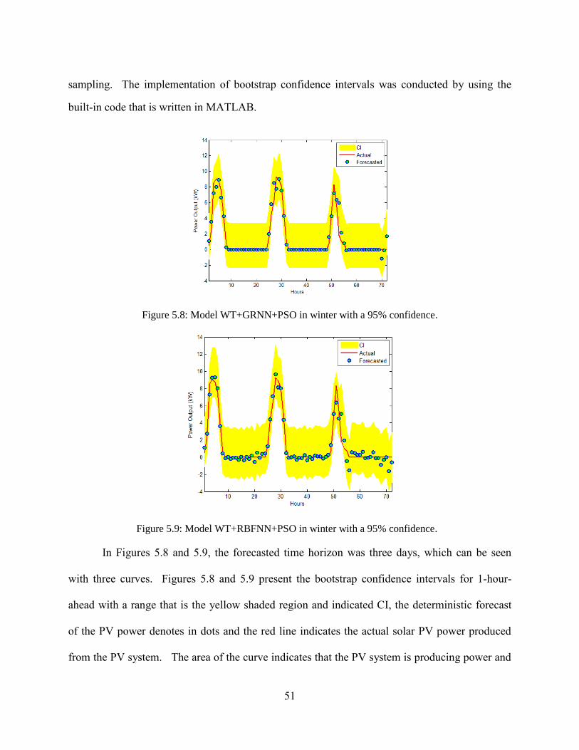
51

sampling. The implementation of bootstrap confidence intervals was conducted by using the

built-in code that is written in MATLAB.

Figure 5.8: Model WT+GRNN+PSO in winter with a 95% confidence.

Figure 5.9: Model WT+RBFNN+PSO in winter with a 95% confidence.

In Figures 5.8 and 5.9, the forecasted time horizon was three days, which can be seen

with three curves. Figures 5.8 and 5.9 present the bootstrap confidence intervals for 1-hour-

ahead with a range that is the yellow shaded region and indicated CI, the deterministic forecast

of the PV power denotes in dots and the red line indicates the actual solar PV power produced

from the PV system. The area of the curve indicates that the PV system is producing power and

52

peaks during midday. Most obvious, the system does not produce any power during the night

time since there is no light; therefore the power remains at zero. The range seems to be much

wider during the night time, this only seems that way due to steep slope of the curves. The

WT+RBFNN+PSO reported lower variation values of uncertainty, thus proving a more robust

model.

Figure 5.10: Bootstrap method for uncertainty estimation at 10%-90% confidence.

WT+RBFNN+PSO was further tested and is shown in Figure 5.10 that presents different

confidence interval percentiles in winter for 1-hour-ahead are shown for comparison ranging

from 10%-90% in darker grey shade to lighter grey shade. The red line also indicates the actual

power produced by the PV power system and the blue lines with dots are the forecasted PV

power output. There is not much variation in the percentages, only that the higher the

confidence percentile, the wider the shaded band. That is, as the confidence level increases, the

wider the interval. The greater the confidence interval, the more uncertainty is covered and

measured. This provides a probability of the deterministic forecast giving a variance. The

advantage of using the bootstrap confidence intervals over the central limit based confidence

53

intervals is that bootstrap provides more uncertainty. The central limit theorem based technique

has a much narrower range of error. Whereas, the range of error is wider using bootstrap

confidence intervals so there is not as much risk giving a broader estimation.

5.5 SUMMARY

In chapter 5, hybrid intelligent models for deterministic and bootstrap method for

uncertainty quantification of solar PV power forecasting was presented. This chapter introduced

the application of GA and PSO to the hybrid intelligent models. The models were extensively

compared by forecasting different day types such as SD, CD, and RD. Then, the variance was

calculated to verify the robustness of the models. Uncertainty estimation was quantified using

bootstrap method and further analysis of the test results2 indicated that WT+RBFNN+PSO is the

superior model.

2 : Findings of this chapter are communicated in conference as indicated below:

D. I. AlHakeem, P. Mandal, A. U. Haque, A. Yona, T. Senjyu, and T. L. B. Tseng, “A new strategy to

quantify uncertainties of wavelet-GRNN-PSO based solar PV power forecasts using bootstrap confidence

intervals,” in Proc. IEEE Power and Energy Society General Meeting, 2015.

54

Chapter 6: Conclusions and Recommendations for Future Work

6.1 GENERAL

The final and concluding chapter of this thesis is divided into three major sections that

are the (i) summary and conclusions, (ii) contributions, and (iii) recommendations for future

work. The summary and conclusions section supports the findings of the study to justify the

objectives of this thesis. The contribution section outlines on the major contributions of this

thesis and the final section provides recommendations for further research based on the

difficulties and experience gained from this thesis.

6.2 SUMMARY AND CONCLUSIONS

This thesis performed STPVF of a solar PV system that is located in Ashland, Oregon by

utilizing various SCMS and hybrid intelligent algorithms. Publicly available data was used to

conduct the forecast at various forecasting horizons and lag times. A summary of this thesis is

outlined below.

Chapter 2 presented a literature review of various techniques applied to solar and wind as

VER by utilizing deterministic forecasting and uncertainty estimation in the form of a

probabilistic forecast. Issues that occur with the PV power generation forecast were

compared and discussed. The factors impacting solar power generation and the

significance of the VERs were presented.

Chapter 3 presented a background of the forecasting methods applied in this thesis was

provided. The preprocessing data filtering technique using WT was explicated.

Learning SCMs utilized to conduct the STPVF were discussed providing the NN

architecture, which were improved through optimization algorithms. Uncertainty

quantification was described utilizing two uncertainty methods, (i) central limit theorem

and (ii) bootstrap confidence intervals.

Chapter 4 applied several deterministic approaches to forecast solar PV power

generation. A method was proposed in this chapter by combining WT with a SCM based

55

on GRNN. Input data was applied that was represented as PV, R, and T. The schematic

forecasting framework of WT+GRNN was presented and the results were discussed.

Accuracy measurement indicated the deterministic forecasted results of WT+GRNN was

the superior model.

Chapter 5 presented STPVF using hybrid intelligent models for deterministic forecasting

and bootstrap method for uncertainty quantification. The integration of GA and PSO to

the hybrid intelligent models was introduced. The models were extensively compared by

forecasting different day types such as SD, CD, and RD. Then, the variance was

calculated to verify the robustness of the models. Uncertainty estimation was quantified

using bootstrap method and further analysis of the test results indicated that

WT+RBFNN+PSO is the superior model.

6.3 CONTRIBUTIONS

This thesis contributed to alleviate an important problem of renewable energy

forecasting, particularly solar PV power generation forecasting. Several developed

methodologies have following characteristics and the development of these methods were major

contributions to this thesis:

The application of the data filtering technique, WT, improved the spike and chaotic

changes in solar PV power time-series data.

SCMs work well with the non-linear solar PV power fluctuation in a significant way.

Optimization algorithm enhances the performance of the SCMs utilized in this study.

A new uncertainty quantification method based on bootstrap confidence intervals was

introduced, which is the first time that this method is used in the solar PV power

forecasting field.

This thesis contributed to develop a hybrid intelligent WT+RBFNN+PSO model and

combine the bootstrap confidence intervals making this thesis novel.

56

6.4 RECOMMENDATIONS FOR FUTURE WORK

There are several factors that were not accounted for in this thesis, which could be

considered for future work. In the forecast, inputs that were considered were solar irradiance,

temperature, and historical PV power generation. For the future, other influencing parameters

could be considered recommendations for future work can be summarized as:

humidity

rainfall

the angle of the PV panels

cloud tracking methods through GPS

other optimization algorithms to optimize the SCMs

integrating solar PV forecasting into electricity market operations to perform

various studies such as security constrained unit commitment, demand response

analysis, and impact on electricity prices

57

References

[1] U.S. Energy Information Administration, Utility-scale installations lead solar photovoltaic growth, [Online].

Available: http://www.eia.gov/todayinenergy/detail.cfm?id=8570.

[2] T. Hong, J. Wilson and J. Xie, “Long term probabilistic load forecasting and normalization with hourly

information,” IEEE Trans. on Smart Grid, vol. 5, no. 1, pp. 456-462, January 2014.

[3] P. Mandal, T. Senjyu, N. Urasaki, A. Yona, T. Funabashi and A. K. Srivastava, “Price forecasting for day-ahead

electricity market using recursive neural network,” in Proc. IEEE Power Engineering Society General Meeting,

2007.

[4] P. Mandal, A. U. Haque, S. T. S. Madhira and D. I. Al-Hakeem, “Applying wavelets to predict solar PV output

power using generalized neural network,” North American Power Symposium (NAPS), 2013.

[5] H. Quan, D. Srinivasan and A. Khosravi, “Short-term load and wind power forecasting using neural network-

based prediction intervals,” IEEE Trans. on Neural Networks and Learning Systems, vol. 25, no. 2, pp. 303-315,

2014.

[6] A. Khosravi, S. Nahavandi and D. Creighton, “Prediction intervals for short-term wind farm power generation

forecasts, IEEE Trans. on Sustainable Energy, vol. 4, no. 3, pp. 602-610, 2013.

[7] (2014 April) Annual Energy Outlook 2014 with projections to 2040 [Online]. Available:

http://www.eia.gov/forecasts/aeo/pdf/0383(2014).pdf.

[8] D. Renne, R. George, S. Wilcox, T. Stoffel, D. Meyers and D. Heimiller, National Renewable Energy

Laboratory, Solar resource assessment, [Online]. Available: http://www1.eere.energy.gov/solar/pdfs/42301.pdf.

[9] (2013 October) NREL, Accuracy of Solar Power Forecasting, [Online]. Available:

http://www.nrel.gov/docs/fy14osti/60142.pdf.

[10] (2012, Oct.) University of Oregon, Solar Radiation Monitoring Laboratory website: [Online]. Available:

http://solardat.uoregon.edu/index.html.

[11] (2014 September) Solar and Wind Forecasting, [Online]. Available:

http://www.nrel.gov/electricity/transmission/resource_forecasting.html.

58

[12] A. U. Haque, M. H. Nehrir and P. Mandal, “A hybrid model for deterministic and quantile regression approach

for probabilistic wind power forecasting,” IEEE Trans. on Power Systems, vol. 29, no. 4, pp. 1663-1672. 2014.

[13] Y. Huang, J. Lu, C. Liu, X. Xu, W. Wang and X. Zhou, “Comparative study of power forecasting methods for

PV stations,” in Proc. International Conference on Power System Technology (POWERCON), 2010.

[14] A. Bossavy, A. Michiorri, R. Girard and G. Kariniotakis, “The impact of available data history on the

performance of photovoltaic generation forecasting models,” in Proc.22nd

International Conference on

Electricity Distribution, 2013.

[15] H.-T. Yang, C.-M. Huang, Y.-C. Huang and Y.-S. Pai, “A weather based hybrid method for 1-day ahead hourly

forecasting of PV power output,” IEEE Trans. on Sustainable Energy, 2014.

[16] B. Tuyishmire, R. McCann and J. Bute, “Evaluation of a Kalman predictor approach in forecasting PV solar

power generation,” in Proc. 4th

IEEE International Symposium on Power Electronics for Distributed

Generation Systems, 2013.

[17] S. Gupta, D. Srinivasan and T. Reindl, “Forecasting solar and wind data using dynamic neural network

architectures for a micro-grid ensemble,” in Proc. IEEE Symposium on Computational Intelligence Applications

in Smart Grid, 2013.

[18] V. P. Singh, V. Vijay, M. S. Bhatt and D. K. Chaturvedi, “Generalized neural network methodology for short

term solar power forecasting,” in Proc. International Conference on Environmental and Electrical Engineering,

2013.

[19] O. Yazdanbaksh, A. Krahn and S. Dick, “Predicting solar power output using complex fuzzy logic,” in Proc.

Joint IFSA World Congress and NAFIPS Annual Meeting, 2013.

[20] D. M. Quan, E. Ogliari, F. Grimaccia, S. Leva and M. Mussetta, “Hybrid model for hourly forecast of

photovoltaic and wind power,” in Proc. IEEE International Conference on Fuzzy Systems,” 2013.

[21] Y. Yang and L. Dong, “Short-term PV generation system direct power prediction model on wavelet neural

network and weather type clustering,” in Proc. 5th

International Conference on Intelligent Human-Machine

Systems and Cybernetics, 2013.

[22] M. Cococcioni, E. D’Andrea and B. Lazzerini, “24-hours-ahead forecasting of energy production in solar PV

systems,” in Proc. 11th

International Conference of Intelligent Systems Design and Applications, 2011.

59

[23] C. S. Ioakimidis, S. Lopez, K. N. Genikomsakis, P. Rycerski and D. Simic, “Solar production forecasting based

on irradiance forecasting using artificial neural networks,” in Proc. 39th

Annual Conference of the IEEE

Industrial Electronics Society, 2013.

[24] J. Kou, J. Liu, Q. Li, W. Fang, Z. Chen, L. Liu and T. Guan, “Photovoltaic power forecasting based on artificial

neural network and meteorological data,” IEEE Region 10 Conference, 2013.

[25] A. Yona, T. Senjyu, T. Funabashi and C.-H. Kim, “Determination method of insolation prediction with fuzzy

and applying neural network for long-term ahead PV power output correction,” IEEE Trans. on Sustainable

Energy, vol. 4, no. 2, pp. 527-533, 2013.

[26] E. G. Kardakos, M. C. Alexiadis, S. I. Vagropoulos, C. K. Simoglou, P. N. Biskas and A. G. Bakirtzis,

“Application of time series and artificial neural network models in short-term forecasting of PV power

generation,” 48th

International Universities’ Power Engineering Conference (UPEC), 2013.

[27] N. Al-Messabi, L. Yun, I. El-Amin and C. Goh, “Forecasting of photovoltaic power yield using dynamic neural

networks,” in Proc. The 2012 International Joint Conference on Neural Networks, 2012.

[28] R. H. Inman, H. T. C. Pedro and C. F. M. Coimbra, “Solar forecasting methods for renewable energy

integration,” Progress in Energy and Combustion Science, vol. 39, no. 6, pp. 535-576, 2013.

[29] K. H. Clifford, S. S. Khalsa, and G. J. Kolb, “Methods for probabilistic modeling of concentrating solar power

plants,” Solar Energy, vol. 85, no. 4, pp. 669-675, April 2011.

[30] S. V. Chakraborty, S. K. Shukla and J. Thorp, “Optimizing grid contribution and economic returns from solar

generators by managing the output uncertainty risk,” in Proc. IEEE Trondheim PowerTech, 2011.

[31] K. Bhaskar and S. N. Singh, “AWNN-assisted wind power forecasting using feed-forward neural network,”

IEEE Trans. on Sustainable Energy, vol. 3, no. 2, pp. 306-315, 2012.

[32] H. Iranmanesh, M. Abdollahzade, A. Miranian and A. Farmahinim “Wind power forecasting by a new local

quadratic wavelet neural network,” in Proc. the International Joint Conference on Neural Networks, 2012.

[33] X. Weidong, L. Yibing and L. Xingpei, “Short-term forecasting of wind turbine power generation based on

genetic neural network,” in Proc. 8th

World Congress on Intelligent Control and Automation, 2010.

60

[34] W. Xiaomei, W. Fushuan, H. Binzhuo, P. Xiangang and H. Jiansheng, “Radial basis function neural network

based on short-term wind power forecasting with grubbs test,” in Proc. 4th

International Conference on

Technologies, 2011.

[35] S. Jie, D. Zhaohao, L. Wei-Jen, Y. Yongping, L. Yongqian and Z. Mingming, “Hybrid forecasting model for

very-short term wind power forecasting based on grey relational analysis and wind speed distribution features,”

IEEE Trans. on Smart Grid, vol. 5, no. 1, pp. 521-526, 2014.

[36] Z. Wei, S. M. Liu, D. Wei, Z. J. Wang, M. L. Yang and Y. Li, “Probabilisitc wind power forecast using sparse

Bayesian learning of unified kernel function,” in Proc. IEEE Conference and Expo Transportation

Electrification Asia-Pacific, 2014.

[37] E. Lorenz, J. Hurka, D. Heinemann and H. G. Beyer, “Irradiance forecasting for the power prediction of grid-

connected photovoltaic systems,” IEEE Journal of Selected Topics in Applied Earth Observations and Remote

Sensing, vol. 2, no. 1, pp. 2-10, 2009.

[38] A. Khosravi, S. Nahavandi, and D. Creighton, “Prediction Intervals for Short-Term Wind Farm Power

Generation Forecasts,” IEEE Trans. on Sustainable Energy, vol. 4, no. 3, pp. 602-610, July 2013.

[39] H. Quan, D. Srinivasan, A. Khosravi, “Short-Term Load and Wind Power Forecasting Using Neural Network-

Based Prediction Intervals, IEEE Trans. on Neural Networks and Learning Systems, vol. PP, no. 99, 2013.

[40] R. Jiang, J. Wang, and Y. Guan, “Robust Unit Commitment With Wind Power and Pumped Storage Hydro,”

IEEE Trans. on Power Systems, vol. 27, no. 2, pp. 800-810, May 2012.

[41] R. J. Bessa, V. Miranda, A. Botterud, J. Wang, and E. M. Constantinescu, “Time Adaptive Conditional Kernel

Density Estimation of Wind Power Forecasting,” IEEE Trans. on Sustainable Energy, vol. 3, no. 4, pp. 660-

669, Oct. 2012.

[42] R. J. Bessa, J. Mendes, V. Miranda, A. Botterud, J. Wang, and Z. Zhou, “Quantile-copula density forecast for

wind power uncertainty modeling,” in. Proc. IEEE Tronheim PowerTech, 2011.

[43] K. Methaprayoon, C. Yingvivatanapong, W. J. Lee, and J. R. Liao, “An Integration of ANN Wind Power

Estimation Into Unit Commitment Considering the Forecast Uncertainty,” IEEE Trans. on Industry Application,

vol. 43, no. 6, pp. 1441-1448, 2007.

61

[44] P. Pinson and G. Kariniotakis, “On-line assessment of prediction risk for wind power production forecasts,”

Wind Energy, vol. 7, no. 2, pp. 119-132, 2004.

[45] W. Can, X. Zhao, P. Pinson, D. Z. Yang and W. K. Po, “Probabilistic forecasting of wind power generation

using extreme learning machine,” IEEE Trans. on Power Systems, vol. 29, no. 3, pp. 1033-1044, 2014.

[46] S. Cros, O. Liandrat, N. Sebastien and N. Schmutz, “Extracting cloud motion vectors from satellite images for

solar power forecasting,” in Proc. IEEE International Geoscience and Remote Sensing Symposium, 2014.

[47] Solar Energy Industries Association, Potential Impact of Solar PV on Electricity Markets in Texas, [Online].

Available: http://www.seia.org/research-resources/potential-impact-solar-pv-electricity-markets-texas.

[48] Electricity Market and Policy Group, Renewable Energy, [Online]. Available: http://emp.lbl.gov/research-

areas/renewable-energy.

[49] A. Mohapatra, M. K. Mallick, B. K. Panigrahi, Z. Cui and S. Hong, “A hybrid approach for short term

electricity price and load forecasting,” in Proc. Conference on International Energy, Automation, and Signal,

2011.

[50] O. A. S. Youssef, “Online Applications of Wavelet Transforms to Power System Relaying,” IEEE Trans.

Power Del., vol. 18, no. 4, pp. 1158- 1165, 2003.

[51] M. Negnevitsky, “Artificial Intelligence,”A Guide to Intelligent Systems, 2nd

ed. England, 2005, pp.1-187

[52] A. Haque, P. Mandal, J. Meng, M. Kaye and L. Chang, “A new strategy for wind speed forecasting using hybrid

intelligent models,” in Electrical and Computer Engineering (CCECE), 2012 25th Canadian Conference on,

Apr.-May 2012.

[53] J. Y. Wu, “Advanced simulated annealing-based BPNN for forecasting chaotic time series,” in Proc.

International Conference on Electronics and Information Engineering, vol. 1, pp. V1-38 – V1-43, 2010.

[54] Mathworks, Radial Basis Neural Networks [Online]. Available:

http://www.mathworks.com/help/nnet/ug/radial-basis-neural-networks.html.

[55] Mathworks, Generalized Regression Neural Networks [Online]. Available:

http://www.mathworks.com/help/nnet/ug/generalized-regression-neural-networks.html.

[56] K. Meng, Z. Y. Dong and K. P. Wong, “Self-adaptive radial basis function neural network for short-term

electricity price forecasting,” IET Generation, Transmission, & Distribution, vol. 3, no. 4, pp. 325-335, 2009.

62

[57] W. C. Hong, C. Y. Lai, W. M. Hung and Y. Dong, “Electric load forecasting by SVR with chaotic ant swarm

optimization,” in Proc. IEEE Conference on Cybernetics and Intelligent Systems, 2010.

[58] Y. Tai-shan, “An improved genetic algorithm and its blending application with neural network,” in Proc. 2nd

International Workshop on Intelligent Systems and Applications, 2010.

[59] X. Wu, “A density adjustment based particle swarm optimization learning algorithm for neural network design,

in Proc. Int. Conf. on Electrical and Control Engineering, 2011.

[60] R. D. Yates and D. J. Goodman, “Confidence Intervals,” in Probability and Stochastic Processes, 2nd

ed.,

Hoboken, John Wiley & Sons, 2005, ch. 7, sec. 7.4, pp. 286-291.

[61] A. Khosravi, S. Nahavandi, D. Creighton and R. Naghavizadeh, “Uncertainty Quantification for wind farm

power generation,” in Proc. International Joint Conference on Neural Networks, 2012.

[62] E. Zio, “A study of the bootstrap method for estimating the accuracy of artificial neural networks in predicting

nuclear transient processes,” IEEE Trans. on Nuclear Science, vol. 53, no. 3, pp. 1460-1478, 2006.

[63] A. Khosravi, S. Nahavandi, D. Srinivasan and R. Khosravi, “Constructing optimal prediction intervals by using

neural networks and bootstrap method,” IEEE Trans. on Neural Networks and Learning Systems, 2014.

[64] L. Gao, R. Shouxin and H. Zahng, “Simultaneous spectrophotometric determination of O-nitro-aniline, M-nitro-

aniline and P-nitro-aniline using a wavelet-based generalized regression neural network,” in Proc. International

Workshop on Modeling, Simulation, and Optimization, pp. 84-87, Dec. 2008.

[65] A. Mellit, M. Benghanem and S. Kalogirou, “An adaptive waveletnetwork model for forecasting daily total

solar-radiation,” Applied Energy, vol. 83, no. 7, pp. 705 – 722, 2006.

[66] A. Khosravi, S. Nahavandi, D. Creighton and D. Srinivasan, “Optimizing the quality of bootstrap-based

prediction intervals,” in Proc. of International Joint Conference on Neural Networks, 2011.

[67] Mathworks, bootci [Online]. Available: http://www.mathworks.com/help/stats/bootci.html.

63

Appendix I

Neural Network Inputs

All models to conduct the solar PV forecast utilized NNs. The NNs applied in this thesis

are BPNN, GRNN, or RBFNN or hybridized the model by combining the NN with WT or

combining the NN with WT and an optimization algorithm, i.e. PSO or GA. Table AI.1 presents

the input parameters that were specifically set in the NNs, which was coded in MATLAB and

remained the same throughout all the models.

Table AI.1: Input parameters for any models that used BPNN, GRNN, and RBFNN.

Parameters BPNN GRNN RBFNN

Activation functions in

hidden layer

tansig radbas radbas

Activation function in

output layer

purelin purelin purelin

Training function trainlm Not Applicable Not Applicable

Momentum 0.4 Not Applicable Not Applicable

Learning Coefficient 1 Not Applicable Not Applicable

Hidden Layer Neurons 6 50 50

Input Neurons 5 9 9

Output Neurons 1 1 1

Epochs 750 50 50

64

In order to conduct the solar PV forecast, various lag times were observed as well as the

forecasting horizon. These values were adjusted accordingly to the season and random days

chosen. Table AI.2 presents these adjusted times that was applied to the forecasted days chosen

that are found in Table 5.1 and associated Tables 5.2-5.4. For example, PVt, is the PV power,

and t is the current time. PVt-16 is the 16 hour lag time and PVt-20 is the 20 hour lag time. Similarly

with R, that signifies the solar radiation and T represents temperature.

Table AI.2: Input time parameters for Tables 5.2-5.4.

Season Day Forecasting

Horizon

Time Lags

Winter D1 8 PVt-1, PVt-16, PVt-20, Rt-1, Rt-16, Rt-20, Tt-1, Tt-16, Tt-20

D2 9 PVt, PVt-15, PVt-20, Rt, Rt-15, Rt-20, Tt, Tt-15, Tt-20

Fall D1 11 PVt, PVt-14, PVt-18, Rt, Rt-14, Rt-18, Tt, Tt-14, Tt-18

D2 8 PVt, PVt-16, PVt-18, Rt, Rt-16, Rt-18, Tt, Tt-16, Tt-18

Summer D1 12 PVt, PVt-12, PVt-24, Rt, Rt-12, Rt-24, Tt, Tt-12, Tt-24

D2 12 PVt, PVt-12, PVt-24, Rt, Rt-12, Rt-24, Tt, Tt-12, Tt-24

Spring D1 12 PVt, PVt-12, PVt-24, Rt, Rt-12, Rt-24, Tt, Tt-12, Tt-24

D2 11 PVt, PVt-12, PVt-20, Rt, Rt-12, Rt-20, Tt, Tt-12, Tt-20

65

Similar to Table AI.2, the solar PV forecast is conducted using various lag times were

observed as well as the forecasting horizon. These values were adjusted accordingly to the

season and type of days chosen. Table AI.3 presents these adjusted times that was applied to the

forecasted days chosen that are found in Table 5.5 and associated Tables 5.6-5.14.

Table AI.3: Input time parameters for Tables 5.6-5.14.

Season Day Forecasting

Horizon

Time Lags

Winter SD 8 PVt, PVt-16, PVt-20, Rt, Rt-16, Rt-20, Tt, Tt-16, Tt-20

CD 8 PVt, PVt-16, PVt-20, Rt, Rt-16, Rt-20, Tt, Tt-16, Tt-20

RD 8 PVt, PVt-16, PVt-20, Rt, Rt-16, Rt-20, Tt, Tt-16, Tt-20

Fall SD 11 PVt, PVt-14, PVt-18, Rt, Rt-14, Rt-18, Tt, Tt-14, Tt-18

CD 11 PVt, PVt-14, PVt-18, Rt, Rt-14, Rt-18, Tt, Tt-14, Tt-18

RD 11 PVt, PVt-14, PVt-18, Rt, Rt-14, Rt-18, Tt, Tt-14, Tt-18

Summer SD 12 PVt, PVt-12, PVt-24, Rt, Rt-12, Rt-24, Tt, Tt-12, Tt-24

CD 12 PVt, PVt-12, PVt-24, Rt, Rt-12, Rt-24, Tt, Tt-12, Tt-24

RD 12 PVt, PVt-12, PVt-24, Rt, Rt-12, Rt-24, Tt, Tt-12, Tt-24

Spring SD 12 PVt, PVt-12, PVt-22, Rt, Rt-12, Rt-22, Tt, Tt-12, Tt-22

CD 12 PVt, PVt-12, PVt-24, Rt, Rt-12, Rt-24, Tt, Tt-12, Tt-24

RD 12 PVt, PVt-12, PVt-24, Rt, Rt-12, Rt-24, Tt, Tt-12, Tt-24

66

The optimization algorithm, GA, was initialized with several input parameters and was

coded in MATLAB. Although, this algorithm used a random number generator function in the

code it had to begin with several inputs to begin.

Table AI.4: GA input parameters for solar PV forecasts.

Parameter Value

Initial Population Size 150

Mutation 30

Best Population 10

Maximum Number of Iterations 50

The optimization algorithm, PSO, was initialized with several input parameters and was

coded in MATLAB. Although, this algorithm used a random number generator function in the

code it had to begin with several inputs to begin.

Table AI.5: PSO input parameters for solar PV forecasts.

Parameter Value

Initial Swarm Size 5

Initial Weight 0.6

Coefficients 1.4

Maximum Number of Iterations 1000

67

Appendix II

Sample MATLAB Code for Back-propagation Neural Network

Different codes were written in MATLAB for each forecasting model such as BPNN,

RFBNN, GRNN including those for WT and optimiztion algorithms (PSO and GA) applied to

forecast the solar PV power generation. The extent of all codes are rather long for each model,

so the following code in Appendix II only provides a partial amount of the BPNN model to

demonstrate an example.

xls_in = 'Ashland_2011.xlsx';

sheetname = 'Sheet1';

range1 = sprintf('D3:D%d',no_rows+1);

range2 = sprintf('E3:E%d',no_rows+1);

range3 = sprintf('F3:F%d',no_rows+1);

Read_data(:,1) = xlsread(xls_in,sheetname,range1);

Read_data(:,2) = xlsread(xls_in,sheetname,range2);

Read_data(:,3) = xlsread(xls_in,sheetname,range3);

PVout = Read_data(data_starting_hour:data_ending_hour,2);

global_radiation = Read_data(data_starting_hour:data_ending_hour,2);

avg_temp = Read_data(data_starting_hour:data_ending_hour,2);

N = length(PVout);

p_input=[];

q_input=[];

for i=ippl:-1:1

test_input_PVout=PVout(N-th-fh+i-ippl:N-fh+i-ippl-1);

p_input=test_input_PVout;

q_input=[q_input p_input];

68

end

test_input_PVout_all=q_input;

test_input_PVout=[test_input_PVout_all test_input_PVout_all(:,Pt2)

test_input_PVout_all(:,Pt3)];

p_input=[];

q_input=[];

for i=ipgl:-1:1

test_input_global_radiation=global_radiation(N-th-fh+i-ipgl:N-fh+i-ipgl-1);

p_input=test_input_global_radiation;

q_input=[q_input p_input];

end

test_input_global_radiation_all=q_input;

test_input_global_radiation=[test_input_global_radiation_all test_input_global_radiation_all(:,Rt2)

test_input_global_radiation_all(:,Rt3)];

p_input=[];

q_input=[];

for i=iptl:-1:1

test_input_avg_temp=avg_temp(N-th-fh+i-iptl:N-fh+i-iptl-1);

p_input=test_input_avg_temp;

q_input=[q_input p_input];

end

test_input_avg_temp_all=q_input;

test_input_avg_temp=[test_input_avg_temp_all test_input_avg_temp_all(:,Tt2)

test_input_avg_temp_all(:,Tt3)];

test_input=[test_input_PVout test_input_global_radiation test_input_avg_temp];

test_target=PVout(N-th:N-1);

tsi=[test_input_PVout test_input_global_radiation test_input_avg_temp];

69

tsd=test_target;

training_input_PVout=PVout(N-th-fh-nn-fh:N-th-fh-1-fh);

p_input=[];

q_input=[];

for i=ippl:-1:1

training_input_PVout=PVout(N-th-fh-nn-fh+i-ippl:N-th-fh-fh+i-ippl-1);

p_input=training_input_PVout;

q_input=[q_input p_input];

end

training_input_PVout_all=q_input;

training_input_PVout=[training_input_PVout_all training_input_PVout_all(:,Pt2)

training_input_PVout_all(:,Pt3)];

p_input=[];

q_input=[];

for i=ipgl:-1:1

training_input_global_radiation=global_radiation(N-th-fh-nn-fh+i-ipgl:N-th-fh-fh+i-ipgl-1);

p_input=training_input_global_radiation;

q_input=[q_input p_input];

end

training_input_global_radiation_all=q_input;

training_input_global_radiation=[training_input_global_radiation_all

training_input_global_radiation_all(:,Rt2) training_input_global_radiation_all(:,Rt3)];

p_input=[];

q_input=[];

for i=iptl:-1:1

training_input_avg_temp=avg_temp(N-th-fh-nn-fh+i-iptl:N-th-fh-fh+i-iptl-1);

p_input=training_input_avg_temp;

70

q_input=[q_input p_input];

end

training_input_avg_temp_all=q_input;

training_input_avg_temp=[training_input_avg_temp_all

training_input_avg_temp_all(:,Tt2) training_input_avg_temp_all(:,Tt3)];

training_input=[training_input_PVout training_input_global_radiation

training_input_avg_temp];

training_target=PVout(N-th-fh-nn:N-th-fh-1);

ti=training_input;

td=training_target;

P=ti';

T=td';

F1='tansig';

F2='purelin';

net=newff(minmax(P),[S1,S2],{F1,F2}, 'trainlm');

net = init(net);

[net,tr]=train(net,P,T);

Y = sim(net,P);

P2=tsi';

T2=tsd';

Y_test = sim(net,P2);

71

Appendix III

List of Abbreviations

AEMO – Australian Energy Market Operator

ANFIS – Adaptive Neuro-Fuzzy Inference System

ANN – Artificial Neural Network

ARIMA – Auto-Regressive Integrated Moving Average

BPNN – Backpropagation Neural Network

CD – Cloudy Day

ECMWF – European Centre for Medium-Range Weather

EIA – Energy Information Administration

GA – Genetic Algorithm

GARCH – Generalized Auto-Regressive Heteroskedastic

GRNN – Generalized Regression Neural Network

H – High Pass Filter

L – Low Pass Filter

MAE – Mean Absolute Error

MAPE – Mean Absolute Mean Percentage Error

NN – Neural Network

NMAE – Normalized Mean Absolute Error

NRMSE – Normalized Root Mean Square Error

PSO – Particle Swarm Optimization

PV – Photovoltaic

R – Global Solar Radiation

RBFNN – Radial Basis Function Neural Network

RD – Rainy Day

72

RGGI – Regional Green-house Gas Initiative

RMSE – Root Mean Square Error

SCM – Soft Computing Model

SD – Sunny Day

STPVF – Short-term PV Forecasting

T – Temperature

t – Time

VER – Variable Energy Resource

WT – Wavelet Transform

73

Appendix IV

PC Technical Specifications

The codes were rather extensive and simulating the codes varied in timing. The codes

were simulated on a PC and Appendix IV presents the technical specifications of the PC utilized.

The simulation time average for BPNN, WT+BPNN, WT+BPNN+GA, and WT+BPNN+PSO

was less than five minutes. The simulation time for GRNN, WT+GRNN, WT+GRNN+GA, and

WT+GRNN+PSO averaged about less than three minutes or less. The simulation time for

RBFNN, WT+RBFNN, WT+RBFNN+GA, and WT+RBFNN+PSO averaged approximately 54

seconds to one minute. Simulations were performed on MATLAB 2010a.

Table AIV.1: PC technical specifications and details.

Specifications Details

PC Brand Lenovo

Processor Intel I7-4500U 1.8-2.4 GHz

RAM 4 GB

Screen Resolution 1600 x 900

Operating System Windows 8 (64-bit)

Disk Space 425 GB

74

Vita

Donna I. AlHakeem was born in Dhahran, Saudi Arabia and moved to the U.S. when she

was 3 years old. She is the first female in her family and a second generation electrical engineer,

correspondingly to her father, to have received a Bachelor of Science in Electrical Engineering,

which she received in 2011 from the University of Texas at El Paso (UTEP).

In early 2013, she pursued her Master of Science in Electrical Engineering (M.S.E.E). In

June of 2013, she started pursuing her research career as a Research Assistant for Dr. Paras

Mandal who advised her throughout her research career and mentored her in the field of power

and energy systems engineering. Before starting this research, she did not have prior knowledge

of the power systems field, particularly in planning and operations. During this period, she

gained extensive research skills and knowledge about power and energy systems. Her skills have

been expanded into publishing research articles in the IEEE conferences where she holds a

student membership since 2013.

1. P. Mandal, A. U. Haque, S. T. S. Madhira, D. I. AlHakeem, “Applying Wavelets to

Predict Solar PV Output Power Using Generalized Regression Neural Network,” in

Proceedings of the North American Power Symposium (NAPS), 2013.

2. D. I. AlHakeem, P. Mandal, A. U. Haque, T. L. B. Tseng, “Smart Electricity Market

Planning and Operation in a Demand Responsive Environment,” in Proceedings of the

4th

Southwest Energy Science and Engineering Symposium, 2014.

3. D. I. AlHakeem, P. Mandal, A. U. Haque, A. Yona, T. Senjyu, T. L. B. Tseng, “A New

Strategy to Quantify Uncertainties of Wavelet-GRNN-PSO Based Solar PV Power

Forecasts Using Bootstrap Confidence Intervals,” in Proceedings of the IEEE Power

and Energy Society General Meeting, 2015. (under review)

The research she conducted as a Research Assistant inspired her toward the completion of

her M.S.E.E. thesis. She continued as a Research Assistant for one full year completing her time

in June 2014.

75

In March 2014, she started her internship position at the local power utilities, El Paso

Electric (EPE), in the Corporate Planning and Development Division. In June 2014, she was

then offered a permanent position at EPE as Economist in the same division where she currently

works. She would like to express her utmost gratitude for the education, knowledge, and

research opportunity she gained while attending UTEP. Additionally, she would like to convey

appreciation to her advisor, Dr. Paras Mandal, for mentoring her in the power and energy

research path. This proceeded to the direct implementation and accomplishment of her research

and M.S.E.E. thesis entitled “Solar PV Power Generation Forecasting Using Hybrid Intelligent

Algorithms and Uncertainty Quantification Based on Bootstrap Confidence Intervals” and

employment at EPE.

Permanent address: 5352 Country Oaks

El Paso, Texas, 79932

This thesis/dissertation was typed by Donna I. AlHakeem.