Solid Mechanics Lecture Notes - Harvard John A. Paulson ...people.seas.harvard.edu/~colinrmeyer/Solid Mechanics Notes.pdf · Solid Mechanics Lecture Notes Colin Meyer Contents 1 Lecture

Solid MechanicsLecture Notes

Colin Meyer

Contents

1 Lecture on 4 September 2013 2


3 Lecture on 9 September 2013 33.1 Generalized Force Balance . . . . . . . . . . . . . . . . . . . . . . . . . . . . . . . . . . . 4



6 Lecture on 16 September 2013 56.1 Steel Plates and Rubber Example . . . . . . . . . . . . . . . . . . . . . . . . . . . . . . . 6


8 Lecture on 20 September 2013 78.1 Stress Concentration Factor . . . . . . . . . . . . . . . . . . . . . . . . . . . . . . . . . . 78.2 Helmholtz Free Energy . . . . . . . . . . . . . . . . . . . . . . . . . . . . . . . . . . . . . 8

9 Lecture on 25 September 2013 109.1 2D Elasticity . . . . . . . . . . . . . . . . . . . . . . . . . . . . . . . . . . . . . . . . . . 10

10 Lecture on 7 October 2013 1010.1 Plane Stress . . . . . . . . . . . . . . . . . . . . . . . . . . . . . . . . . . . . . . . . . . . 1010.2 Airy Stress Function . . . . . . . . . . . . . . . . . . . . . . . . . . . . . . . . . . . . . . 11

11 Lecture on 9 October 2013 1211.1 Plane Strain . . . . . . . . . . . . . . . . . . . . . . . . . . . . . . . . . . . . . . . . . . . 12

12 Lecture on 11 October 2013 1312.1 Sinusoidal Loading on a Half Space . . . . . . . . . . . . . . . . . . . . . . . . . . . . . . 1312.2 Saint-Venant’s Principle . . . . . . . . . . . . . . . . . . . . . . . . . . . . . . . . . . . . 1512.3 Circular Cavity Plane Stress . . . . . . . . . . . . . . . . . . . . . . . . . . . . . . . . . . 15

13 Lecture on 16 October 2013 1613.1 Cut and Weld Operation . . . . . . . . . . . . . . . . . . . . . . . . . . . . . . . . . . . . 1613.2 Remote Shear Loading . . . . . . . . . . . . . . . . . . . . . . . . . . . . . . . . . . . . . 17

14 Lecture on 18 October 2013 1814.1 Line Force . . . . . . . . . . . . . . . . . . . . . . . . . . . . . . . . . . . . . . . . . . . . 18

15 Lecture on 21 October 2013 1815.1 Dynamics: Vibration and Waves . . . . . . . . . . . . . . . . . . . . . . . . . . . . . . . . 18

16 Lecture on 23 October 2013 20

17 Lecture on 25 October 2013 2017.1 Reflection and Transmission . . . . . . . . . . . . . . . . . . . . . . . . . . . . . . . . . . 21

1

18 Lecture on 28 October 2013 2218.1 Plane Waves . . . . . . . . . . . . . . . . . . . . . . . . . . . . . . . . . . . . . . . . . . . 22

19 Lecture on 30 October 2013 2419.1 Slowness Surface . . . . . . . . . . . . . . . . . . . . . . . . . . . . . . . . . . . . . . . . 24

20 Lecture on 1 November 2013 24

21 Lecture on 4 November 2013 2421.1 Viscoelasticity . . . . . . . . . . . . . . . . . . . . . . . . . . . . . . . . . . . . . . . . . . 24

22 Lecture on 6 November 2013 2522.1 Active Load . . . . . . . . . . . . . . . . . . . . . . . . . . . . . . . . . . . . . . . . . . . 26

23 Lecture on 8 November 2013 2623.1 Relaxation Test . . . . . . . . . . . . . . . . . . . . . . . . . . . . . . . . . . . . . . . . . 2623.2 Cyclic Test . . . . . . . . . . . . . . . . . . . . . . . . . . . . . . . . . . . . . . . . . . . 27

24 Lecture on 11 November 2013 2824.1 Finite Deformation . . . . . . . . . . . . . . . . . . . . . . . . . . . . . . . . . . . . . . . 28

24.1.1 Homogeneous Deformation . . . . . . . . . . . . . . . . . . . . . . . . . . . . . . . 28



27 Lecture on 22 November 2013 3127.1 Stress in Homogeneous Deformation . . . . . . . . . . . . . . . . . . . . . . . . . . . . . . 3127.2 Material Model and Thermodynamics . . . . . . . . . . . . . . . . . . . . . . . . . . . . . 32

28 Lecture on 25 November 2013 3328.1 Inhomogeneous Deformation . . . . . . . . . . . . . . . . . . . . . . . . . . . . . . . . . . 3328.2 Rubber Elasticity . . . . . . . . . . . . . . . . . . . . . . . . . . . . . . . . . . . . . . . . 34


30 Lecture on 4 December 2013 3530.1 Necking . . . . . . . . . . . . . . . . . . . . . . . . . . . . . . . . . . . . . . . . . . . . . 35

1 Lecture on 4 September 2013

Introduction to solid mechanics.


In this course on solid mechanics we will only consider the linear part of the stress/strain relationship. Stressand strain are defined as

Stress = σ =Force

Areaand Strain = ε =

Elongation

Length.

Linear elasticity is a material model or a constitutive law. Now we consider the experiment of uniaxialforce. In the linear regime, we find that

σ = Eε,

where E is Young’s modulus, which is a material property. This only really makes if the material ishomogeneous, which means that material properties do not vary with spatial position. To specify whethera material is homogeneous requires at least two lengthscales: a macroscopic lengthscale L and a microscopiclengthscale a. Material homogeneity means that L� a. These material properties can also be defined forcomposites, but then the properties refer to the materials together and not separately.

2

For a cube in an arbitrary state of stress, that is known, we are curious what are the strains. Fromgeneralized Hooke’s law we have that

εxx =σxxE− νσyy

E− νσzz

E,

εyy =σyyE− νσxx

E− νσzz

E,

εzz =σzzE− νσxx

E− νσyy

E.

Here we have used the same homogeneous, isotropic, and linear assumptions.For the same cube we can now think about the shear stress τ and shear strain γ. If a shear stress is

applied to the cube, the angle that the cube makes with the vertical is called the shear strain γ, and is underthe small angle approximation. It is important to remember that solid body rotation is not strain.

Balancing forces on a rectangle of sides a, b, and c gives

τ1(ac) = τ3(ac) −→ τ1 = τ3 and τ2(ab) = τ3(ab) −→ τ2 = τ4.

Balancing moments gives that

τ1(abc) = τ2(abc) −→ τ1 = τ2 = τ3 = τ4 = τ.

All of the forces that we encounter in solid mechanics are surface, body, and inertial forces. If we considera small enough body we can ignore gravity. Experiments show that

τ = µγ,

where µ is the shear modulus.


Starting with a square, of side length a, under arbitrary stress we have, in the x-direction

εx =σxE− νσy

E− νσz

Eand γxy =

σxyµ.

Now we want to show that

µ =E

2(1 + ν),

under the assumptions that the body is homogeneous, isotropic, and linear.If we rotate the square by 45◦, we are in the same state of stress, except that we can now relabel the

forces. Cutting a small right triangle from the bottom corning of the square we have the force balance

√2aσ =

τa√2

+τa√

2−→ σ = τ.

By geometry, we can examine the square before and after deformation. The initial side lengths are a, andthe hypotenuse is

√2. The top left corner moves in by γa, using the small angle approximation. Thus, the new

hypotenuse can be found to be√a2 + a2(1− γ)2. Using the fact that γ is very small, we find that the strain is

ε =

√a2 + a2(1− γ)2 −

√2a√

2a≈√

1− γ − 1 ≈ −γ2.

From force balance we haveε = − σ

E− ν σ

E.

Inserting the fact that σ = τ and ε = −γ/2, we have that

γ

2=

1 + ν

Eτ ←→ τ = µγ,

3

where

µ =E

2(1 + ν).

Generalized Hooke’s Law can be written using engineering strain γ, which is related to scientific strain ε as

γxy = 2εxy.

This can be succinctly written in tensor notation as

εij =(1 + ν)

Eσij −

ν

Eσkkδij.

This can be inverted to give the stress in terms of the strain. Taking the trace of the last equation we have

εii =(1 + ν)

Eσii − 3

ν

Eσkk =

(1− 2ν)

Eσii −→ σii =

E

(1− 2ν)εii.

For i 6= j, we have that

σij =E

1 + νεij.

Thus, the stress equation must be of the form

σij =E

1 + νεij + λεkkδij.

It is important to note that the stress tensor is symmetric, i.e., σij = σji. Taking the trace and insertingthe trace from before we have

σii =E

(1− 2ν)εii =

E

1 + νεii + 3λεkk.

This can be rearranged to give

λ =Eν

(1− 2ν)(1 + ν).

Inserting the definition of the shear modulus, we find the stress/strain relationship

σij = 2µεij + λεkkδij,

where µ and λ are called Lame’s constants.Temperature effects can be incorporated into the analysis by writing the strain as

εij =1

2µσij −

ν

Eσkkδij + α∆T,

where α is the coefficient of expansion.

3.1 Generalized Force Balance

Here we develop an approach to deal with problems of arbitrary forces on arbitrary bodies. By examining thestate of stress for a material particle, we can determine the forces. To do this we only need 6 quantities (less than9 due to symmetry); these are the six sides of a cube. We can see this by a simple counting argument: 6 planeson a cube and 3 directions gives 18 forces. But, normal stresses form 3 pairs and shear stress form 3 quadruples.

For an arbitrary body under force, we can cut a plane through the body and examine the forces on thatplane. The force per area on that plane is called the traction, ti, and is given by

ti = σijnj,

where nj is the vector normal to the plane.

4


This lecture started with a description of the conventions for stress notation and directions. In σij, the i givesthe direction of force and j is the direction of the normal to the plane. Thus, for a cube with one corner at theorigin, the shear σyz, points vertically (positively) on the positive yz face and negatively on the opposite side.

Now about tensors. It is important to remember that

δkk = 3.

A quadratic form isq = xTBy (scalar).

Any B of this form is a tensor. Therefore, if we can show that

ti = σijnj,

is true, then σij is a tensor. Balancing forces in the x-direction gives

Atx = Axσxx +Ayσxy +Azσxz.

Dividing by A, givestx = nxσxx + nyσxy + nzσxz,

which is the expression we were looking for, and thus, σij is a tensor.


Now we consider the stress concentration in an inhomogeneous field. To do this we must exam a materialparticle that is homogeneous. An example of this sort of problem is a sheet with a hole in it that is under anapplied stress. The hole has radius a. Now to have a homogeneous particle we have that the lengthscale of theparticle p is much greater than the atomic spacing b, but much smaller than the hole size a, i.e., a� p� b.

The way to develop the PDE is to examine the interactions between material particles. A few importantfields are the displacement ui, which is inhomogeneous, the stress field σij, and an appropriate body force bi.There is also the density ρ. Drawing a material particle of size dx, dy, and dz we can compute the changein stress and find that

ρ∂2ui∂t2

=∂σij∂xj

+ bj.

Compatibility between material particles requires that

εxx =∂ux∂x

, εyy =∂uy∂y

, εzz =∂uz∂z

.

Including the diagonal components, this can be generalized to

εij =1

2

(∂ui∂xj

+∂uj∂xi

).


In a model for the deformation of a solid, there are three components: a material model, a force balance,and the geometry of deformation. Each of these represents an equation. In this class, the equations are

σij = 2µεij + λεkkδij (material model). (1)

ρ∂2ui∂t2

=∂σij∂xj

+ bj. (force balance). (2)

εij =1

2

(∂ui∂xj

+∂uj∂xi

)(geometry of deformation). (3)

Counting equations we can see that there are enough equations for all of the unknowns. The unknownsare: 3 for the displacement field, ui, 6 for the stress field σij and also 6 for the strain field εij. This gives15 unknowns. The material model is 6 equations, the force balance is 3 equations, and the geometry ofdeformation is 6 more equations, which is 15, the required number.

Many solid mechanics problems are boundary value problems, which means that to fully solve the problem weneed boundary conditions. For the static case, i.e. no initial conditions, the two main boundary conditions are:

5

(a) Prescribed displacement at the boundary. This is where ui is given at part of the surface of the body.

(b) Prescribed traction ti, which is the force per area, on part of the surface of the body. For a material particle,one can only apply three directions of stress, i.e., the traction. The entire stress tensor cannot be prescribed!

Now to solve these problems one can either, use a computer (i.e., Finite Element Analysis), use a handbookof common solutions, or try to find an analytic or approximate solution. Now we will do an example.

6.1 Steel Plates and Rubber Example

Consider a thin piece of rubber squished between two steel plates. There is an applied normal stress in thevertical direction and no shear. Thus, σzz = σA and σxx = σyy. In this analysis we will ignore edge effects andassume that the steel is perfectly bonded to the rubber, so no sliding, the steel is rigid so all the strain is carriedin the rubber, and the stress and strain fields are homogeneous. Since the strain in the x-direction is zero we have

εxx =1

E(σxx − νσyy − νσzz) −→ σxx = σyy =

(ν

1− ν

)σzz.

There is no shear stress so σxy = σxz = σyz = 0. Now we want to determine the strain in the verticaldirection, thus we write

εzz =1

E[σzz − ν (σxx + σyy)] =

1

E

[σzz −

(2ν2

1− ν

)σzz

]=

1

E

[σzz −

(2ν2

1− ν

)σzz

]=

1

E

(1− ν − 2ν2

1− ν

)σzz.

Rubber is nearly incompressible, meaning that ν ≈ 1/2 or physically that shape changes do not lead tosignificant volume changes. If we insert ν = 1/2, we find that

σxx = σyy = σzz and εzz = 0.

This is hydrostatic compression.


This lecture introduced the ideas of stress concentration around imperfections and characterizing them witha Stress Concentration Factor. Many more of the details of this analysis were presented in the next lecture.

At the start of the lecture there was an important discussion of the size restriction on the imperfections.Mirroring the earlier discussion of homogeneous, we must consider two lengthscales: L is the large, “sample”size and b is the atomic size. Our analysis requires that a, the size of the imperfection, satisfies b� a� L.

We can also see that the stress concentration factor is size independent. To see why this is, note thatthe equations have no specific lengthscale and that the stress field is linear in the applied load as

σyy = σAf(xa,y

a

).

An example of this, is the stress right at the edge of an elliptic curve in a thin sheet, stressed vertically, is given as

σyy = σA

(1 + 2

a

b

).

Now an easier BVP is to solve for the stress concentration is in an axisymmetric geometry, where there isa circular hole of radius a. Here the stress, strain, and displacement all only depend on the radial coordinate,r. This dramatically simplifies the equations. To derive the expression of force balance, we consider a freebody diagram where we balance forces in the r direction. Choosing two points, one at r and one at r + dr,we can write the balance as

−σθ(r)2πrdr− σr(r)πr2 + σr(r+ dr)π[r+ dr]2 = 0.

Keeping only first order terms, we have that

−σθ(r)2πrdr− σr(r)πr2 + σr(r+ dr)πr2 + σr(r+ dr)2πrdr = 0.

Dividing through we have that

2−σθ(r) + σr(r+ dr)

r+σr(r+ dr)− σr(r)

dr= 0.

6

Sending dr→ 0, we find thatdσrdr

+ 2σr − σθ

r= 0.

We can also derive the strain/displacement relation. The radial strain is given as

εr =du

dr.

The radial strain can be derived as

εθ =2π(r+ u)− 2πr

2πr=u

r.


8.1 Stress Concentration Factor

Here we consider the problem of an axisymmetric geometry with a hole of size a cut out of it. Our threeingredients are

(1) Material Model: εr =1

E(σr − 2νσθ) and εθ =

1

E(σθ − νσθ − νσr)

(2) Deformation Geometry: εr =du

drand εθ =

u

r

(3) Force Balance:dσrdr

+ 2σr − σθ

r= 0.

We can eliminate u by solving for the strains as

u = rεθ −→ εr =d

dr(rεθ)

. This is often referred to as the compatibility relation. Then inserting the material model into the compatibilityrelation gives

σr − 2νσθ = σθ − νσθ − νσr + r

(dσθdr− νdσθ

dr− νdσr

dr

).

We can simplify this equation to

(1 + ν)σr = (1 + ν)σθ + r(1− ν)dσθdr− νrdσr

dr.

Solving the force balance for σθ as

σθ = σr +r

2

dσrdr

and inserting it into the expanding compatibility relation gives

(1 + ν)σr = (1 + ν)σr + (1 + ν)r

2

dσrdr

+ r(1− ν)dσrdr

+r

2(1− ν)

dσrdr

+r2

2(1− ν)

d2σrdr2− νrdσr

dr.

After a few simplifications we have

0 = rdσrdr

+ r(1− ν)dσrdr

+r2

2(1− ν)

d2σrdr2− νrdσr

dr.

This simplifies further to

0 = 2r(1− ν)dσrdr

+r2

2(1− ν)

d2σrdr2

.

Finally, we arrive at

d2σrdr2

+4

r

dσrdr

= 0.

Notice that both Poisson’s ratio and Young’s modulus canceled out. Since this is a second order ODE weneed 2 boundary conditions. These are

7

1. Stress at edge (far-field) r→∞ is σr = σA, which is the applied stress.

2. At the surface of the cavity, the traction (vector acting on a surface) vanishes. Thus, at r = a, σr = 0.

We can write these boundary conditions as

σr =

{σA, r→∞0, r = a

.

The ODE is an equi-dimensional equation, which means that there are the same number of r’s in each term.This is strong indication that the equation admits a power-law type solution of the form

σr ∼ rα.

Inserting this into the ODE, we have

(α− 1)αrα−2 + 4αrα−2 = 0 −→ α(α+ 3) = 0.

Thus, the radial stress is given as

σr = A+B

r3.

Inserting the boundary conditions we find that

σr(r→∞) = A = σA and σr(r = a) = 0 −→ B = −a3A.

Thus,

σr = σA

(1− a3

r3

).

Now to find the stress concentration factor we need to compute the axial stress, σθ at r = a. We can findthe axial stress from the force balance relation; thus,

σθ = σr +r

2

dσrdr

= σA

[1 +

1

2

(ar

)3].

The stress concentration factor is the maximum nondimensional stress. That is, if we nondimensionalizethe radial and axial stress components, as

σr = σAΣr and σθ = σAΣθ for the radial coordinate r = aR.

This gives the equations,

Σr = 1− 1

R3and Σθ = 1 +

1

2R3,

on the intervalR = [1,∞]. The maximum stress comes from the axial stress atR = 1, so therefore, we have that

Stress Concentration Factor, SCF = Σmax =σmaxσA

= Σθ(R = 1) =3

2.

8.2 Helmholtz Free Energy

Consider a bar that is deformed from the length L0 and area A0 to a new length L and area A. The differencein length is given as δL = L− L0. For a fixed temperature and a bar deformed slowly, we can write thework W done by the force P in increasing the length by δL as

W = PδL.

Thus, the energy stored in the bar is elastic. To do this correctly, we need to write the Helmholtz Free EnergyδF as

δF = PδL,8

which we can interpret by saying that an elastic body in thermodynamic equilibrium (with environmentat a constant temperature T), the work done by the force equals the change in Helmholtz free energy.

Considering the stress/strain we can write,

Stress: σ =P

A0

and Strain: ε =L−L0

L0

.

Hence, using the definitions, we have

PδL = σA0δεL0 = σδεV0,

where V0 = A0L0. Thus, we can writeδW = σδε,

with δW as the Helmholtz free energy per volume. Rearranging, and at a constant temperature, we findthe the important relation

σ =∂W

∂ε.

Now considering Shear, we see that the work for a cube of side length H and angle of deformation γ isPHδγ. Following the same, arguments gives

τ =∂W

∂γ.

Combining these two definitions and generalizing to a multiaxial stress state, we have

δW = σijδεij and thus σij =∂W

∂εij, (4)

remembering that γij = 2εij for i 6= j. For anisotropic materials, constructing stress/strain relations in amultiaxial stress state, requires the specification of each component of stress as a function of six componentsof strain. The outcome may or may not satisfy thermodynamics. For Helmholtz Free Energy, only needto specify one function of all six strains and it automatically satisfies thermodynamics.

We will assume an anisotropic body but with a linear stress/strain relation – therefore, W is a quadraticform of the six strains. Writing the strain components as a single vector as

ε = [ε11, ε22, ε33, ε23, ε13, ε12],

and the stress equivalently. Here we for the last three components we have used the “missing number entryscheme,” where since in the fourth element it is the first shear, the number 1 is left out. Following a similarconvention, this strain can also be written as

ε = [ε1, ε2, ε3, ε4, ε5, ε6].

Using the previous convention, and assuming Einstein summation convention, the most general quadraticform of W is

W =1

2Cijklεijεkl.

This is identical two writing it as

W =1

2cpqεpεq.

Since cpq = cqp, we know that there can only be 21 distinct elastic constants; here p and q go from 1 to 6.The stress/strain relation can then be computed from equation (4) as

σij =1

2Cijklεkl or σp =

1

2cpqεq.

For a cubic lattice, there is cubic symmetry and thus will only have 3 independent constants.9


Picking up from last time, the function W is the Helmholtz Free Energy per unit volume, it is a scalar, anda quadratic form of εij. For an isotropic material, there are only two material constants.

The mathematical idea in determining the general form of W is to consider the tensor invariants of εij.The three invariants of second rank tensor Tij are

(1) Tii (2) TijTij and (3) TjkTikTij.

We know that W is a quadratic form and it is an invariant because it does not change with coordinaterotation. The most general case is then

W = αεijεij + β (εkk)2 .

For isotropic materials, we can identify α and β as α = µ, the shear modulus, and β = [E − 2µ]/[2(1− 2ν)].

9.1 2D Elasticity

Pulling a thin sheet, there will be no bending, therefore we can assume that the body will be in plane stress.This means that

σzz = 0 and σxz = σyz = 0.

From this we can ascertain that,

εxz = εyz = 0 though εzz 6= 0.

All the other stresses and strains are function of x and y only.

10 Lecture on 7 October 2013

10.1 Plane Stress

Here we consider a plane stress problem where all of the forces are in the plane. Furthermore, we have thatσzz = σyz = σxz = 0. Writing out the (1) material model, (2) deformation geometry, and (3) force balance,we find that

εzz =∂w

∂z= f(x, y) −→ w = zεzz + g(x, y).

Furthermore,

εxz =1

2

(∂u

∂z+∂w

∂z

)= 0 −→ ∂w

∂x= 0 −→ ∂εzz

∂x= −g

z.

Integrating gives

εzz = −1

z

∫gdx+ h(y, z).

In doing this analysis, we assumed that εzz was not a function of z. The only way to prevent this is to set

h(y, z) =1

z

∫gdx. −→ εzz = 0.

This means that there is no z dependence in any equation and the equations reduce to 2D equations ofmotion. Writing them out we have

εxx =1

E(σxx − νσyy) , εyy =

1

E(σyy − νσxx) , εxy =

(1 + ν

E

)σxy,

εxx =∂u

∂x, εyy =

∂v

∂y, εxy =

1

2

(∂u

∂y+∂v

∂x

),

∂σxx∂x

+∂σxy∂y

= 0,∂σxy∂x

+∂σyy∂y

= 0.

These are 8 equations for 8 unknowns.

10

10.2 Airy Stress Function

A theorem in calculus states that if

f =∂p

∂yand g =

∂p

∂x,

then∂f

∂y=∂g

∂x.

This can be easily proved by showing that

∂f

∂y=

∂2p

∂x∂y=∂g

∂x,

and since mixed partials are equal, it must be true. Interestingly, and unsurprisingly, the inverse is alsoalways true. That is, if

∂f

∂x=∂g

∂y,

we can always find a p such that

f =∂p

∂yand g =

∂p

∂x.

Applying this to the force balance equation,

∂σxx∂x

= −∂σxy∂y

,

we can find a function A such that

σxx =∂A

∂yand σxy = −∂A

∂x.

from the other equation, we have that

∂σyy∂y

= −∂σxy∂x−→ σxy = −∂B

∂yand σyy =

∂B

∂x.

Since we know that the stress tensor is symmetric, we have the equation

σxy = σyx −→∂A

∂x=∂B

∂y.

Hence, we can apply the theorem again to find the function φ, such that

A =∂ϕ

∂yand B =

∂ϕ

∂x.

This gives the three relationships

σxx =∂2ϕ

∂y2, σxy = − ∂2ϕ

∂x∂y, and σxx =

∂2ϕ

∂x2.

The function ϕ is the Airy Stress Function.Now we need to find a single PDE for ϕ. We cannot use force balance as that has already been used.

Writing the stress/strain relations in terms of ϕ, we have

εxx =1

E

[∂2ϕ

∂y2− ν∂

2ϕ

∂x2

], εxy = −

(1 + ν

E

)∂2ϕ

∂x∂y, and εyy =

1

E

[∂2ϕ

∂x2− ν∂

2ϕ

∂y2

].

11

Deformation geometry gives

εxx =∂u

∂x, εyy =

∂v

∂y, and εxy =

1

2

(∂u

∂y+∂v

∂x

).

Taking mixed derivatives of the shear strain and displacement relation we have

∂2εxy∂x∂y

=1

2

(∂2

∂y2∂u

∂x+

∂2

∂x2∂v

∂y

),

thus, we can eliminate u and v to give

∂2εxy∂x∂y

=1

2

(∂2εxx∂y2

+∂2εyy∂x2

).

Inserting the stress/strain relations into the deformation geometry equation just derived, we have

−(

1 + ν

E

)∂4ϕ

∂x2∂y2=

1

2E

(∂4ϕ

∂y4− ν ∂4ϕ

∂x2∂y2+∂4ϕ

∂x4− ν ∂4ϕ

∂x2∂y2

).

Rearranging gives∂4ϕ

∂y4− 2ν

∂4ϕ

∂x2∂y2+∂4ϕ

∂x4+ 2 (1 + ν)

∂4ϕ

∂x2∂y2= 0.

Thus, we find a single PDE for ϕ, as

∂4ϕ

∂y4+ 2

∂4ϕ

∂x2∂y2+∂4ϕ

∂x4= 0.

This equation is the Biharmonic equation, and just as the name implies, can be written as

∇4ϕ = 0 ←→(∂2

∂x2+

∂2

∂y2

)(∂2ϕ

∂x2+∂2ϕ

∂y2

)= 0.


For plane stress problems we have an excellent PDE for a single function ϕ, from which the stresses andstrains can be computed. The difficulty now is to determine the boundary conditions. The most commonboundary conditions are

1. Traction Free: Stress vanishes, σrr = σrθ = 0. An example of traction free boundary conditions arefree boundaries or at a hole.

2. Prescribed Traction: On a curve or at certain place in space, t = σ ·n. This leads to two equations for ϕ.

3. Prescribed Displacement: u is a fixed value at a single or several locations in space. The stress mustbe solved for first and then integrated to give the displacement.

11.1 Plane Strain

If the geometry and load are such that they are invariant in the z-direction, meaning zero displacement inz direction or w = 0, then the plane strain approximation can be used. This means that the displacementin the x and y directions (u and v respectively) are not functions of z and only functions of x and y.

Writing out the three ingredients we have

εxx =1

E(σxx − νσyy − νσzz) , εyy =

1

E(σyy − νσxx − νσzz) ,

εzz =1

E[σzz − ν (σxx + σyy)] , εxy =

(1 + ν

E

)σxy,

εxx =∂u

∂x, εyy =

∂v

∂y, εxy =

1

2

(∂u

∂y+∂v

∂x

), εzz = 0,

∂σxx∂x

+∂σxy∂y

= 0,∂σxy∂x

+∂σyy∂y

= 0.12

Since there is no displacement in the vertical direction, there is no strain. This allows us to write the verticalstress as

σzz = ν (σxx + σyy) .

Inserting this into the stress/strain relationships we have

εxx =1

E

[(1− ν2

)σxx − ν(1 + ν)σyy

], εyy =

1

E

[(1− ν2

)σyy − ν(1 + ν)σxx

], and εxy =

(1 + ν

E

)σxy.

Pulling out common factors from each term, we can write these equations as

εxx =1− ν2

E

[σxx −

(ν

1− ν

)σyy

], εyy =

1− ν2

E

[σyy −

(ν

1− ν

)σxx

], and εxy =

(1 + ν

E

)σxy.

Defining E and ν as

E =E

1− ν2and ν =

ν

1− ν,

we can convert the equations to the form

εxx =1

E[σxx − νσyy] , εyy =

1

E[σyy − νσxx] , and εxy =

(1 + ν

E

)σxy,

which is exactly the same form as for plane stress. Thus, the Airy Stress Function approach will also workfor plane strain.


12.1 Sinusoidal Loading on a Half Space

Here we consider the problem of sinusoidal loading along the x = 0 line in the halfspace x ∈ [0,∞). Theload is given as

σxx(x = 0, y) = σ0 cos

(2πy

λ

)and σxy(x = 0, y) = 0,

which serves as the boundary conditions at x = 0. We expect that the stress should decay away for x� λ. Ad-ditionally, the applied force averages to zero over a period. This is the first indication of Saint-Venant’s Principle.

The governing partial differential equation is the biharmonic equation for the Airy Function ϕ, which isgiven as

∂4ϕ

∂x4+

∂4ϕ

∂x2∂y2+∂4ϕ

∂y4= 0.

Because this is a linear equation, we will look for solutions of the form

ϕ = f(x)g(y).

Based on the boundary conditions, it is reasonable to expect that

g(y) = cos

(2πy

λ

)−→ ϕ = f(x) cos

(2πy

λ

).

Inserting this into the biharmonic equation yields

f ′′′′ cos

(2πy

λ

)− 2f ′′

(2π

λ

)2

cos

(2πy

λ

)+ f

(2π

λ

)4

cos

(2πy

λ

)= 0.

We can label 2π/λ as k, cancel the cosines, and write the ODE

f ′′′′ − 2k2f ′′ + k4f = 0.

13

The boundary conditions on f are

σxx(x = 0, y) =∂2ϕ

∂y2

∣∣∣∣x=0

= σ0 cos

(2πy

λ

)−→ −k2f(x = 0) = σ0,

σxy(x = 0, y) =∂2ϕ

∂x∂y

∣∣∣∣x=0

= 0 −→ kf ′(x = 0) = 0.

Thus,

f(x = 0) = −σ0k2

and f ′(x = 0) = 0.

Letting f = Aeαx, we can insert this into the ODE to find that

α4 − 2k2α2 + k4 = 0.

This readily factors to(α2 − k2)2 = 0,

meaning that the roots are α = ±k, but are degenerate. This means that the general solution is

f(x) = Aekx +Be−kx +Cxekx +Dxe−kx.

A slight mathematical diversion can be used to show where the last two terms come from. If we considereαx and eβx as two distinct solutions, then their difference is also a solution. We are then interested in thecase where α→ β. Thus, we can write a solution as

limα→β

eαx − eβx

α− β= lim

α→β

ddα

(eαx − eβx

)ddα

(α− β)= lim

α→βxeαx,

where we have invoked L’Hopital’s rule for indeterminate limits.Back to the general solution for f , we can immediately rule out the solutions that blow up as x→∞,

and therefore we are left withf(x) = Be−kx +Dxe−kx.

Inserting the boundary conditions we have that

f(x = 0) = B = −σ0k2

and f ′(x = 0) =σ0k

+D = 0→ D = −σ0k,

thus,

f(x) = −σ0k2

(1 + kx)e−kx.

The Airy Stress Function is then

ϕ = −σ0k2

(1 + kx)e−kx cos (ky) .

From ϕ we can calculate the stresses as

σxx =∂2ϕ

∂y2= σ0(1 + kx)e−kx cos (ky) .

σyy =∂2ϕ

∂x2= σ0(1− kx)e−kx cos (ky) .

σxy = − ∂2ϕ

∂x∂y= σ0kxe

−kx sin (ky) .

Some things to note about this solution are that, as expected the decay length scales with the wavelength,L ∼ λ. From the full solution we find that L = λ/2π, which is considerably shorter than just the wavelength.Secondly, it is important to note that the stress field is linear in the applied load, σ0, which is a consequenceof linear elasticity.

14

12.2 Saint-Venant’s Principle

If the resultant force and moment of applied load vanish, the field always decays beyond the length overwhich the load is applied. We have already seen several examples of this:

1. For a spherical cavity inside of a large linear elastic medium, we found that the stress decays as

σ ∼ a3

r3,

Hence the stress decays as a power law for r� a. This highlights the fact that the decay need notbe exponential.

2. Some experiments in cells showed that Saint-Venant’s Principle may be wrong in biology. Furtherresearch found that the long stiff Actin fibers can transmit force over longer distances. Professor Suoliken these Actin Fibers to piano wires in tofu.

3. For the problem of rubber (thickness d) between two steel plates, the edge effects can be ignored atgreater than d into the sample.

12.3 Circular Cavity Plane Stress

Here we consider the boundary value problem of a 2D circular hole of radius a in a thin sheet that is loadedin the far field by a stress σA. Due to the symmetry we will use polar coordinates. The radial, axial, andshear stress are related to the Cartesian stresses as

σr =σx + σy

2+

(σx − σy

2

)cos(2θ) + σxy sin(2θ)

σθ =σx + σy

2−(σx − σy

2

)cos(2θ)− σxy sin(2θ)

σrθ = −(σx − σy

2

)sin(2θ) + σxy cos(2θ)

The can be determined by considering the force balances on a triangle at an angle θ from the usual stresscube. In terms of the Airy function ϕ, we have that

σr =1

r2∂2ϕ

∂θ2+

1

r

∂ϕ

∂r, σθ =

∂2ϕ

∂r2, and σrθ = − ∂

∂r

(1

r

∂ϕ

∂θ

).

The biharmonic equation in polar coordinates is given as

∇4ϕ =

(1

r

∂

∂r

(r∂

∂r

)+

1

r2∂2

∂θ2

)(1

r

∂

∂r

(r∂ϕ

∂r

)+

1

r2∂2ϕ

∂θ2

)= 0.

If we assume that ϕ is a function of r only, this simplifies to(1

r

∂

∂r+

∂2

∂r2

)(1

r

∂ϕ

∂r+∂2ϕ

∂r2

)= 0.

This equation is an equidimensional equation and thus the solution is a power law of the form ϕ rm. Insertingthis into the equation we find that(

1

r

∂rm−2

∂r+∂2rm−2

∂r2

)(m+m(m− 1)) = m2(m− 2)2 = 0.

Thus, we again have degenerate roots. The general solution for degenerate roots from a power law is

ϕ = A+B ln(r) + [C +D ln(r)]r2.

15

A similar mathematical diversion shows that this is the correct solution. Considering two solutions of theform rα and rβ, where we expect α→ β. Now, we consider the limit

limα→β

rα − rβ

α− β= lim

α→β

eα ln(r) − eβ ln(r)

α− β= lim

α→β

d

dα

(eα ln(r)

)= lim

α→βln(r)rα.

From the general solution, we can immediately disregard A because only derivatives of ϕ are important. Thestress field is then

σr =1

r

∂ϕ

∂r=B

r2+ 2C + [1 + 2 ln(r)]D,

σθ =∂2ϕ

∂r2= −B

r2+ 2C + [3 + 2 log(r)]D,

σrθ = 0.

The boundary conditions are

σr = 0 on r = a and σr = σA as r→∞.

Therefore, we can see that D = 0, or the stress would be infinite as r→∞. Thus, we have that

C =σA2

and B = −2Ca2 = −σAa2.

This gives the stress field

σr = σA

[1−

(ar

)2],

σθ = σA

[1 +

(ar

)2],

σrθ = 0.

The stress concentration factor can then be easily computed as

SCF =σmaxσA

=2σAσA

= 2.


13.1 Cut and Weld Operation

In the analysis from the previous lecture we disregarded the D term because it blew up as r→∞. Herewe will determine what D 6= 0, means physically. Ignoring all other effects, we can take

ϕ = Dr2 ln(r).

From this, we can calculate the stresses to be

σr =1

r

∂ϕ

∂r= [1 + 2 ln(r)]D,

σθ =∂2ϕ

∂r2= [3 + 2 log(r)]D,

σrθ = 0.

The stresses are axisymmetric with no dependence on the angle θ. This doesn’t provide any clues. The strainfield can be calculated for plane strain as

εr =1

E(σr − νσθ) =

D

E[(1− 3ν) + 2(1− ν) ln(r)] ,

εθ =1

E(σθ − νσr) =

D

E[(3− ν) + 2(1− ν) ln(r)] .

16

This again doesn’t give us any insight. The crucial idea is that the strain and displacement field may notbe axisymmetric. This is weird because the stress fields is axisymmetric; however, if we consider a cut andweld operation, or a disclination, where a small sliver of a circle is removed and then the rest of the materialis stretched and then the sliver is welded together again. This operation leaves a residual strain in the body.From the strain/displacement relation we have that

εr =∂ur∂r

, εθ =urr

+1

r

∂uθ∂θ

, and εrθ =1

r

∂ur∂θ

+∂uθ∂r− ur

r.

Integrating we find that

ur =D

E[2(1− ν)r ln(r)− (1− ν)r] +H sin(θ) +K cos(θ),

uθ =4Drθ

E+ Fr+H cos(θ)−K sin(θ).

The sin(θ) and cos(θ) terms represent rigid body translations and therefore can be ignored, i.e. H = K = 0.The Fr term is a rigid body rotation and can be ignored by setting F = 0. Thus, we have the displacement field

ur =D(1− ν)r

E[2 ln(r)− 1]),

uθ =4Drθ

E.

Now we need boundary conditions in order to solve for D. These are related to the cut and weld processand given as

uθ = 0 for θ = 0 and uθ = αr for θ = 2π,

where α is the angle of the sliver originally cut. Thus,

α =8πD

E−→ D =

αE

8π.

This gives the displacement field

ur =α(1− ν)r

8π[2 ln(r)− 1]),

uθ =αrθ

2π.

In this way, we see that D 6= 0, means that the displacement field is not axisymmetric. If we find that itis indeed axisymmetric, then D = 0.

13.2 Remote Shear Loading

At the end of class, we quickly consider the boundary value problem of remote shear loading on a circularhole of radius a. That is,

r→∞, σxy = S and σx = σy = 0.

Converting these to polar coordinates gives

r→∞, σr = S sin(2θ), σθ = −S sin(2θ), and σrθ = S cos(2θ).

Given, the boundary conditions above, it is reasonable to expect that the Airy Stress Function will be of the form

ϕ = f(r) sin(2θ).

We can insert this into∇4ϕ = 0,

and we find that (∂2

∂r2+

1

r

∂

∂r− 4

r2

)(∂2f

∂r2+

1

r

∂f

∂r− 4f

r2

)= 0.

17

As this is again equidimensional, we can suppose f = rm and we find that m = 2,−2,0,4. Thus there areno degenerate roots. Calculating the stress and applying a traction free boundary at r = a, we find thestress field to be

σr = S

[1− 4

(ar

)2+ 3

(ar

)4]sin(2θ),

σθ = −S[1 + 3

(ar

)4]sin(2θ),

σrθ = S

[1 + 2

(ar

)2− 3

(ar

)4]cos(2θ),


14.1 Line Force

Consider a semi-infinite body subject to a point force P per unit length (2D, constant along the thirddimension). This BVP has no prescribed lengthscale, and thus, the only way to construct a stress is to write

σij =P

rfij(θ).

From the biharmonic equation for the Airy function ϕ and the relationship between ϕ and σ, we have that

f ′′′′ + 2f ′′ + f = 0,

where primes are taken with respect to θ. This readily integrates to give

ϕ = Prf(θ) = Pr [A cos(θ) +B sin(θ) +Cθ cos(θ) +Dθ sin(θ)] .

Because of the symmetry of the problem, we only want symmetric functions. The only symmetric functionsfrom the above expression are cos(θ) and θ sin(θ). But cos(θ) is only a translation and therefore does notcontribute to stress. Thus, we are left with

ϕ = PrCθ sin(θ).

To find the force balance, we can cut a little circle around P. Thus,

ΣFx =

∫ π2

−π2

σrr cos(θ) dθ+ P = 0→ C = −1

π.

This means that

σrr = −2P

πrcos(θ), and σθ = σrθ = 0.

The rest of this lecture was devoted to studying the problem of:S. Ho, C. Hillman, F.F. Lange and Z. Suo, Surface cracking in layers under biaxial, residual compressive

stress, J. Am. Ceram. Soc. 78, 2353-2359 (1995).


15.1 Dynamics: Vibration and Waves

Consider the 1D problem of a block of mass M attached to a spring with constant k. There is no friction.The force balance in this case is

Mx+ kx = 0.

Integrating this equation gives

x(t) = A cos(ωt) +B sin(ωt) where ω =

√k

M.

18

The initial conditions are

x(t = 0) = prescribed and x(t = 0) = prescribed.

For a single rod in one dimension, we can use a continuum model where

σ = Eε, ε =∂u

∂xand ρ

∂2u

∂t2=∂σ

∂x.

Putting all of these pieces together we have that

∂2u

∂t2=E

ρ

∂2u

∂x2.

The initial conditions are

u(x,0) = prescribed and∂u

∂t

∣∣∣∣t=0

= prescribed.

This equation is a wave equation with wave speed c given as

c =

√E

ρ−→ ∂2u

∂t2= c2

∂2u

∂x2.

We can examine the solutions to the wave equation by considering u = f(x) sin(ωt). Inserting this into thewave equation we have that

f ′′ +ρ

Eω2f = 0.

Defining α as

α = ω

√ρ

E,

we have thatf(x) = A cos(αx) +B sin(αx).

We now need to prescribe boundary conditions. Since they are good for all time and always must be satisfied,they are the conditions imposed on f(x). If we consider a fixed displacement at x = 0, and a traction freecondition at x = L, we have that

f(x = 0) = 0 −→ B = 0 and f ′(x = L) = 0.

The second condition implies that

Aω

√ρ

Ecos

(Lω

√ρ

E

)= 0→ Lω

√ρ

E=π

2(2n+ 1) for n = 0,1,2 . . .

Thus, the natural frequencies are given by

ω = (2n+ 1)π

2L

√E

ρ.

This is similar to ω =√k/M. The fundamental mode is given by n = 0, and thus,

ω0 =π

2L

√E

ρ.

19


The beginning of this class was a discussion of a beautiful experiment to show that light doesn’t need a mediumto propagate through, however, sound does: A ticking watch is placed in a vacuum sealed glass jar. The observercan see the hands tick as time passes but since there is no air to move through, the sound cannot be heard.

For nondispersive sound waves, the shape of the wave does not change with time. As an example, if youhit a steel rod with a hammer, a sound wave travels down the rod without changing form.

The wave equation written as∂2u

∂t2= c2

∂2u

∂x2,

admits solutions of the formu = F(x− ct) +G(x+ ct).

We can easily see this by using the variables

ζ = x− ct and η = x+ ct,

then taking the derivatives we have

∂2u

∂t2=

∂2F

∂ζ2

(∂ζ

∂t

)2

+∂2G

∂η2

(∂η

∂t

)2

= c2∂2F

∂ζ2+ c2

∂2G

∂η2.

c2∂2u

∂x2= c2

[∂2F

∂ζ2

(∂ζ

∂x

)2

+∂2G

∂η2

(∂η

∂x

)2]

= c2∂2F

∂ζ2+ c2

∂2G

∂η2.

The velocity of a material particle, different than the wave velocity, is given by

v =∂u

∂t.

The stress, for this 1D system is written as

σ = E∂u

∂x.

Inserting our expressions for u(x, t), we can write the general solution as

u = F(x− ct) +G(x+ ct) = F(ζ) +G(η),

v = −c∂F∂ζ

+ c∂G

∂η,

σ = E∂F

∂ζ+E

∂G

∂η.

Note that at all times the stress is related to the velocity as

σ = −Rv,

where R =√ρE is the acoustic impedence.


The functions F(ζ) and G(η) are determined by initial conditions. Generic initial conditions are

u(x, t = 0) = u(x),

v(x, t = 0) = v(x).

These can be written in terms of the functions F(x) and G(x), since t = 0, as

F(x) +G(x) = u(x),

−cF ′ + cG′ = v(x)20

where the primes indicate differentiation with respect to the traveling wave variable, ζ and η respectively.Multiplying the first expression by c, differentiating, and then solving for G′, and then following a similarprocedure to get F ′, yields the result

F ′ =1

2u′ +

1

2cv,

G′ =1

2u′ − 1

2cv

Inserting these into the initial stress gives

σ(x, t = 0) = EF ′ +EG′ = Eu′,

which shouldn’t be a surprise as that is the definition we used earlier! At a later time, this initial way splitsinto two waves that travel in opposite directions. Thus, the stress is given as

σ(x, t) =E

2

[∂u

∂x

∣∣∣∣x−ct

+∂u

∂x

∣∣∣∣x+ct

].

17.1 Reflection and Transmission

Consider an incident stress wave traveling down a rod that sits along the x-axis in the region x < 0. Atx = 0, there is a free end, so that σ(0, t) = 0. No matter what the wave form is (for nondispersive waves),we can consider linear superposition – by adding in an imaginary bar in the region x > 0, we consider anidentical wave to the incident wave, but manipulate its properties so that the stress-free condition is satisfiedat x = 0. In this case, the sign of the wave must be switched. The wave speed stays the same but the signreverses so as the wave reaches the end the reflected wave with opposite sense cancels out the stress at theend. This has the unintuitive consequence of turning a compressive wave reflect into a tensile wave.

Now we can consider the same set-up except change the boundary condition at x = 0. Imagine insteadif we put a wall at x = 0, which would lead to a fixed end, so that u(0, t) = v(0, t) = 0. In this case, thewave keeps the same sign, but travels in the opposite direction.

These two situations can be seen as the limiting cases to a more general scenario: We have an incidentstress wave traveling in an elastic media with Young’s modulus E1 and density ρ1, which gives wave speedc1 and impedance R1 =

√ρ1E1. At x = 0, the wave encounters another medium with Young’s modulus E2

and density ρ2, which gives wave speed c2and impedance R2 =√ρ2E2. This interface leads to part reflection

and part transmission. We can write the stress and particle velocity as

σ = RF ′(xc− t)−RG′

(−xc− t),

v = −F(xc− t)

+G(−xc− t),

where the functions F and G are arbitrary so we can incorporate factors of c and −1.The three waves we need to keep track of are the incident wave, the reflected wave, and the transmitted

wave. We can hypothesize that the shape of the wave doesn’t change but the amplitudes of the reflectedand transmitted waves have smaller but potentially different amplitudes. Also, we only need to considerone side of the wave because the other one travels away from the interface. Thus, we can write

Incident Wave

σI = RF ′(xc− t),

vI = −F(xc− t),

Reflected Wave

σR = −αRF ′(−xc− t),

vR = −αF(−xc− t),

Transmitted Wave

σT = βRF ′(xc− t),

vT = −βF(xc− t),

21

where α and β are the unknown amplitudes. The signs of the reflect wave are switched as it travels in theopposite direction. The boundary conditions across the interface are

Traction Continuous :: σI + σR = σT on x = 0.

Velocity Continuous :: vI + vR = vT on x = 0.

The terms on the left hand side of the above boundary conditions are in the first medium while the transmittedwave is in the second medium. Inserting the wave forms into the boundary conditions, gives

R1F′ (−t) + αR1F

′ (−t) = βR2F′ (−t) ,

−F ′ (−t)− αF ′ (−t) = −βF ′ (−t) .

Canceling out common factors leaves us with

R1(1− α) = βR2,

1 + α = β.

Solving this equation for α and β gives

α =R1 −R2

R1 +R2

and β =2R1

R1 +R2

.

Now let us examine three limits.

1. R1 = R2: In this limit, we find that α = 0 and β = 1, meaning that the wave is entirely transmitted.This makes sense because R1 = R2 means that there is no material change.

2. R1 � R2: Impedance matched. Here α → 1 and β → 2. Here there will be a reflection but thereflected wave has the opposite sign as the incident wave.

3. R2� R1: This is the limit where the impedance of the second material is negligible and we have only thereflected wave, i.e. α→−1 and β → 0, but the sign of the wave is identical to that of the incident wave.


18.1 Plane Waves

Here we will study a plane wave, the width of the wave is much greater than the amplitude, propagatingparallel to the direction of displacement – a so-called Longitudinal Wave. We consider a homogeneous andisotropic material.

The wave moves in the x-direction and that is the only strain. Due to the Poisson effect there will howeverbe normal stress in all three directions. Thus, the equations are

εx =∂u

∂xand εy = εz = 0,

εx =1

E[σx − ν(σy + σz)] ,

εy = 0 =1

E[σy − ν(σx + σz)] ,

εz = 0 =1

E[σz − ν(σx + σy)] ,

ρ∂2u

∂t2=

∂σx∂x

.

From the fact that the y and z strains are zero we have that

σz = ν(σx + σy) and σy =

(ν

1− ν

)σx.

22

Inserting this into the expression for εx yields

εx =1

E

[(1− ν2

)σx − ν(1 + ν)σy

]=

1

E

[(1− ν2

)− ν(1 + ν)

(ν

1− ν

)]σx =

1

E

[(1 + ν)(1− 2ν)

1− ν

]σx.

Inserting this into the force balance, and writing the strain in terms of the displacement gives

ρ∂2u

∂t2=∂σx∂x

=E(1− ν)

(1 + ν)(1− 2ν)

∂2u

∂t2.

Thus, the wave speed for a longitudinal wave is

cl =

√E(1− ν)

ρ(1 + ν)(1− 2ν).

Another type of wave is a transverse wave, where the direction of displacement is perpendicular to thedirection of propagation. If we consider a simple two dimensional wave, the only nonzero strain is

γxy =∂uy∂x

,

and thus, the only stress is

τxy = µγxy = µ∂uy∂x

.

Inserting this into the force balance gives

∂τxy∂x

= ρ∂2uy∂t2−→ ∂2uy

∂t2=µ

ρ

∂2uy∂x2

.

Thus, the wave equation for a simple transverse wave is

ρ∂2uy∂t2

= µ∂2uy∂x2

.

This gives a wave speed of

ct =

√µ

ρ.

Since

µ =E

2(1 + ν),

we can see that

ct =

√E

2ρ(1 + ν).

This is less than the longitudinal wave speed by a factor of

ct = cl

√(1− ν)

(2− 4ν),

which for small ν, is about

ct 'cl√2

+νcl

2√

2.

A general wave form is written as

Longitudinal :: u = sf

(s · xcl− t),

Longitudinal :: u = ag

(s · xct− t)

+ bh

(s · xct− t),

23

where s is the direction of propagation, a is the direction of displacement and b is another direction ofdisplacement.

For an anisotropic solid we need to change our material model, so that

σij = Cijklεkl,

which is reflected in the new wave equation

Cijkl∂2uk∂xl∂xj

= ρ∂2ui∂t2

,

noting that because of the symmetry in σij, we have that Cijkl = Cjikl. Looking for plane waves, we can write

ui = aif(skxk

c− t),

where c and ai (unit vector) need to be determined and f is the wave form. We also note that sk is a unitvector. Inserting this into the wave equation we have that

Cijklakslsjc2

d2f

dζ2= ρai

d2f

dζ2.

Rearranging and canceling like terms yields

[Cijklslsj]ak = ρc2ai,

which is an eigenvalue problem for ρc2. The term in brackets is called the acoustic tensor and is symmetricand positive definite – this means that there will be three positive real eigenvalues ρc2 with orthogonaleigenvectors ak.


19.1 Slowness Surface

In general the vector sk and its relation to the wave speed c are combined into a quantity called the slowness.In other words sk/c is called the slowness vector. For a fully anisotropic material we learned that the threeeigenvectors of the acoustic tensor are orthogonal and the three eigenvectors are distinct, real, and positive.Now if we plot all of the points, 1/c1, 1/c2, and 1/c3 along each direction sk, and connect all of the firsteigenvalues and the second as well as the third, then each inverse eigenvalue defines a surface. This is calledthe slowness surface. For an isotropic material the slowness surfaces are just two spheres as there are onlytwo slowness vectors (transverse and longitudinal).

20 Lecture on 1 November 2013

Introduction to viscoelasticity.


21.1 Viscoelasticity

Here we consider the creep test: at time t = 0, we hang a weight at the end of a material and record the elonga-tion as a function of time. We consider the output to be a function of elastic components σ = Eε and Newtonianviscous components σ = H∂ε/∂t, where H is the viscosity. Viscoelasticity is the sum of the two effects.

An idealization that we work with in this class is linear viscoelasticity. That is, for time dependent strainε(t), we have that

ε(t) = D(t)σ.

The D(t) is called the creep compliance. This is the case where σ is constant – that prescribed by the weighthanging. What we see in the output is that there is a characteristic timescale for relaxation; i.e. after a timeτ the strain flattens and additional time yields almost no strain. The value of the final strain reached is therelaxed strain, given by εR or for the creep compliance, DR. An interesting phenomenon is that at time t = 0,almost instantaneously, there is a large jump in strain. This is called the unrelaxed strain and given by εU orDU for the creep compliance. The usual fitting formula for linear viscoelastic creep compliance of this form is

D(t) = DR + (DU −DR)e−tτ .

24

It is our goal in this section to relate this model to physics.Two important models are the Maxwell model and the Kelvin model. Unfortunately they do not exactly

work for this case (they apply in different situations). The model that we will use is called the StandardModel or the Zener Model. It consists of a spring and dashpot connected in parallel (constants E1 and H1

respectively) placed in series with another spring (constant E0). Thus, the total strain is given as

ε = ε0 + ε1.

In the unrelaxed state, as t→ 0 the dashpot cannot move, and thus ε1 = 0. Hence, σ = E0ε0, so we can write

εU =σ

E0

and DU =1

E0

,

as σ is a constant. In the fully relaxed state, the dashpot can carry no stress, as ∂ε/∂t = 0, therefore onlythe spring carries load. Hence, we can write

ε = ε0 + ε1 =σ

E0

+σ

E1

= εR,

and thus,

DR =1

E0

+1

E1

.

The relaxation timescale, is the transition from the dashpot in a locked state and to the stress free state.Thus, it is the trade-off between the importance of the spring E1 and the viscosity H1, i.e.

τ =H1

E1

.


In the last lecture we were able to deduce the creep compliance parameters from physical reasoning, butnow we can do it from first principles. From before we have that

ε = ε0 + ε1, ε0 =σ

E0

and σ = E1ε1 +H1∂ε1∂t.

We can readily integrate the last expression to find that

ε1 =σ

E1

(1− e−

E1tH1

).

We can then insert this and the expression for ε0 in the ε expression to find that

ε(t) =σ

E0

+σ

E1

(1− e−

E1tH1

).

Our creep compliance D(t) is then given by

D(t) =1

E0

+1

E1

(1− e−

E1tH1

).

From this we can recognize, that the DU and DR derived last time are indeed correct and that the timescaleis as speculated.

An interesting extension to this analysis is to consider a material with multiple stages of relaxation. Thiscan be accommodated by adding another parallel spring and dashpot (new constants E2 and H2) in serieswith the other parallel spring and dashpot and spring. This gives another timescale τ2 = H2/E2.

25

22.1 Active Load

The final thing is to consider how the strain changes over time with a load that changes over time. The ideathat we use is called the Boltzmann Superposition Principle: this states that we can consider short incrementsof time and think of the stress as constant over that period of time. Writing the creep compliance as

D(ξ) = D(ξ)H(ξ),

where H(ξ) is the Heaviside step function. Using this method, we can write the strain as

ε(t) = σ0D(t− s0) + (σ1 − σ0)D(t− s1) + (σ2 − σ1)D(t− s2) . . .This can accommodate increasing and decreasing stress values. If we send the step size to zero this sumbecomes an integral as

ε(t) =∞∑l=0

(σl+1 − σl)D(t− sl)→ ε(t) =

∫ t

−∞D(t− s)dσ

dsds.

We can therefore find the strain response for a known σ(t), by doing a creep test to determine D(t), andthen doing the integral.


23.1 Relaxation Test

The next topic in viscoelasticity is an experimental test called the relaxation test. Essentially, at time t = 0a step strain is enforced. In other words, at time t = 0, we have that the length instantaneously increasefrom L0 to L. Thus,

ε0 =L−L0

L0

.

We can see that initially this requires significant force and after a time β, another relaxation time, the stressdecreases to a constant value. Surprisingly, the relaxation time β is not the same as τ from the creep test.Luckily, we can continue to model this situation with the Zener model. The only difference is that timethe strain is fixed (imagine between two walls) and the stress varies with time. Thus, the equations are

σ = E1ε1 +H1dε1dt, σ = E0ε0 and ε = ε0 + ε1.

By writing,

ε1 = ε− ε0 = ε− σ

E0

.

Inserting this into the expression for σ and ε1, we find the ODE:

H1

E0

dσ

dt+

(1 +

E1

E0

)σ = E1ε.

Dividing through by the constants in front of the σ, we find the timescale β to be

β =H1

E0 +E1

.

Now, solving this ODE we find that

σ(t) = E0ε+

[E0E1

E0 +E1

−E0

]ε(

1− e−tβ

).

We can immediately recognize

σU = εE0 and σR =E0E1

E0 +E1

ε from σU = E0ε and ε =σRE0

+σRE1

.

We want linear viscoelasticity asσ(t) = E(t)ε,

and thus,

E(t) = E0 +

[E0E1

E0 +E1

−E0

](1− e−

tβ

).

As before EU = E0 because the dashpot is locked and ER is given when the dashpot can carry no stress.26

23.2 Cyclic Test

If we prescribe the strain as a function of time to be

ε(t) = ε0 sin(ωt),

where ω is the angular frequency – ω = 2πf – where f is the inverse of the period. If we assume linearviscoelasticity, the important observation is that the stress has the same form but with a phase shift, i.e.

σ(t) = σ0 sin(ωt+ δ).

There is a slight problem with this solution because σ(t = 0) 6= 0 but ε(t = 0) = 0. This leads naturallyto thinking about the solution as a combination of both elastic modes and viscous modes. If we prescribeε(t) = ε0 sin(ωt) and a linear elastic material model, we find that

σ = Eε(t) = Eε0 sin(ωt),

which doesn’t have a phase shift. But then if we, using the same ε(t), write the stress as

σ = Hdε

dt= Hω cos(ωt) = Hω sin

(ωt+

π

2

).

Thus, for linear viscoelasticity we have that

0 ≤ δ ≤ π

2.

From trigonometry we can decompose the phase shifted stress into

σ(t) = σ0 sin(ωt+ δ) = σ0 [sin(ωt) cos(δ) + cos(ωt) sin(δ)] .

Hence, we can write the first part as the elastic component and the second as the linear viscous component:

σ(t) = [σ0 cos(δ)] sin(ωt) + [σ0 sin(δ)] cos(ωt).

Then, we can write

E′ =σ0ε0

cos(δ) and E′′ =σ0ε0

sin(δ),

where E′ is the storage modulus and E′′ is the loss modulus. The phase shift δ can be given by

δ = arctan

(E′′

E′

)To proceed we will use complex variables. Writing the stress and strain as

ε(t) = ε∗eiωt and σ(t) = σ∗eiωt,

where the starred variables are complex and satisfy

σ∗ = E∗ε∗,

withE∗ = E′ + iE′′.

Writing the stress asσ(t) = σ∗eiωt = E∗ε∗eiωt,

we can decompose E∗ into a generic complex number by writing

E∗ = Eeiδ,

27

and thus,σ(t) = Eε∗eiωt+iδ.

Using the Zener (standard) model, we have the equations

σ = E1ε1 +H1dε1dt, σ = E0ε0 and ε = ε0 + ε1.

Inserting our complex forms gives

σ∗ = E1ε∗1 + iH1ωε

∗1, σ∗ = E0ε

∗0 and ε∗ = ε∗0 + ε∗1.

Solving for the stress gives

σ∗ =

{E0 (E1 + iH1ω)

E0 +E1 + iH1ω

}ε∗.

We can recognize the factor in the curly braces to be E∗. To tease out the real and complex componentsof E∗ in terms of E0, E1, and H1, we must multiply the top and bottom by the complex conjugate of thebottom. This yields

E′ = EU +ER −EU1 + (ωβ)2

and E′′ =(ER −EU)ωβ

1 + (ωβ)2,

where

EU = E0, ER =E0E1

E0 +E1

, and β =H1

E0 +E1

.


24.1 Finite Deformation

24.1.1 Homogeneous Deformation

The engineering strain between the current state (lower case letters) and the reference state (capitol letters).

ε =l−LL

.

The natural strain is

e = ln

(l

L

).

Notation for this quantity may change; later we will use ε. Another important definition is the stretch

λ =l

L.

Notice that the three definitions are related as

e = ln(λ) = ln(ε+ 1) and λ = ee = ε+ 1.

Thus, homogeneous deformation meansy = λY,

is independent of the material particles chosen. In three dimensions there are three components to the stretch,i.e.

λ1 =l1L1

, λ2 =l2L2

, and λ3 =l3L3

.

Now a measure of the homogeneous deformation should independent of the size and shape of both bodies. Ifwe consider Y to be a set of material particles in the reference state and y to be the same material particlesin the current state, we can write

y = FY . (5)

In other words, if the deformation is homogeneous F is independent of Y . If we start with a cube of unitvectors, then after stretching, rotating, and translating each material segment, we find that the new sidevectors make up a parallelopiped and are given as

(e1, e2, e3)→ (Fe1, Fe2, Fe3).

28


Here we continue on finite deformation. For clarity sake, we define y and Y as

Y :: A set of material particles that form straight line segment when the body is the reference state.

y :: The same set of material particles that still form a straight line segment in the current state.

We say that deformation is homogeneous if F is a linear operator, as this preserves the straight segments.The definition of a linear operator is

1. F(Y1 + Y2

)= FY1 + FY2.

2. F (αY ) = αFY1.

Connecting these ideas to actual deformation we can see that the first rule states that the vector that formsthe sum of the two vectors in the reference state is mapped to the sum of the two vectors in the currentstate. The second principle gives the idea that if in the reference state, I have two vectors, one of whichis just a longer version of the other, both pointing the same direction, then in the current state, the deformedvectors can also be scaled in the same way.

Now we know that rigid body motion does not affect the state of matter, so what size and shapeparallelopiped does our deformation give us? To answer this, we need to know the length of each side andthe angle between them (six quantities).

Thus, we can write what is called the Green Deformation Tensor and is given by

C = FTF.

This matrix is symmetric and positive definite. We can easily see that it is symmetric because CT = C.To see that it is positive definite, we must show that

xTCx > 0 −→(Fx)T (

Fx)> 0→ yTy > 0,

where y = Fx 6= 0.Here we consider a vector of length L and unit direction M in the current state and the corresponding

length l and direction m in the reference state. Writing

Y = LM and y = lm,

we have from equation (5) thatlm = LFM.

Taking the inner product of both sides with lm, we have

l2 = L2MTFTFM,

thus,

λ2 = MTCM. (6)

If the original volume of the body in the reference state is V , then the volume in the current state v, isgiven by the curl of the two side lengths dotted with the third. In other words

v = V(Fe1 ∧ Fe2

)· Fe3 = V (εijkFj1Fk2)Fi3 = V εijkFi3Fj1Fk2 = V det(F).

In the last step we used a theorem that relates the determinant of a matrix to the scalar tripe product. Thus,

v = V det(F) .

Similarly, if we consider an area A with normal vector N in the reference state and an area a with normalvector n in the current state, we can write the volume of the enclosed region as

V = AN ·L,29

where L is some height. The corresponding volume in the current state is

v = V det(F) = AN ·Ldet(F).

Since the deformation is homogeneous, we also know that

v = an · l and l = FL.

Combing these two expressions we have

an · FL = AN ·Ldet(F).

Dotting both sides by L, we have

an · F = Adet(F)N and ||n|| = 1.

For a known A, F , and N, these two conditions are sufficient to find a and n.


Considering the same problem we have be examining – a unit square that deforms to a parallelopiped – weknow that rigid body motion or rotation do not cause stress. Thus, we only care about the size and shape ofthe parallelopiped, because these do affect or are affect stress. This is what led us to the Green DeformationTensor, which is

C = FTF.

We can also calculate strain via the Lagrange Strain, which is written as

E =1

2

(C − I

).

In the reference state, the principle directions of deformation in the reference state are those that in thecurrent state give a square. To do this we want to solve an eigenvalue problem. We cannot use F because itcontains extra information about rotation. We can, however, diagonalize C, which is symmetric and positivedefinite, and therefore contains 3 positive and real eigenvalues. The eigenvectors are also orthogonal andmake up the principle directions in the reference state. The eigenvalues are given as

CM = αM.

From equation (6), we can writeλ2 = MTCM = MTαM,

and thus,λi =

√αi.

Thus, we are able to determine the length of the principle stretches.Now ifM1 andM2 are orthogonal eigenvectors in the reference state, we want to show that the corresponding

vectors m1 and m2 in the current state are also orthogonal. Writing

λ1m1 = FM1 and λ2m2 = FM2,

we can dot them together to find that

λ1λ2m1Tm2 = FTM1

TFM2 = M1TCM2 = αM1

TM2 = 0,

thus, we can see that m1 and m2 are indeed orthogonal.What about the rotation contained in F? We can consider a writing F as a product of two matrices, one

that has only shape change and one that accounts for the rotation. This is called the polar decompositionand is given by

F = RU.

30

Now we can examine what we know already about the matrices U and R. Because R represents only rotationand no shape change, the determinant must be unity. A property of matrices with unity determinant arethat they satisfy

RT = R−1 −→ RTR = RRT = I.

This is called an orthogonal matrix. We can also see that U is symmetric and positive definite. Because

F is nonsingular, FTF is a positive definite and symmetric matrix. Hence, we can find a positive definiteand symmetric operator such that

FTF = U2.

Furthermore, we can also see that FU−1 is an orthogonal operator, so that(FU−1

)T (FU−1

)=(U−1FT

) (FU−1

)= UU2U−1 = I.

Thus, we have shown that the matrices U and R satisfy the requirements stipulated. Since,

C = MTAM and C = U2,

where A is the matrix with eigenvalues on the diagonal and M is the matrix of eigenvectors. we have that

U = MTAM,

where

A =√A.

Now we can find R as

R = FUT .


27.1 Stress in Homogeneous Deformation

Two common definitions of stress in mechanics are

Nominal Stress :: s =P

Aand True Stress :: σ =

P

a,

where P is the force, A is the area in the reference state, and a is the area in the current state. In finitedeformation, we can generalize the nominal stress to

P = sAN,

where s is a linear map. The nominal traction T is given as

T = sN =P

A.

We can see that the forces balance but because the forces are not aligned the torques do not. For two forcesP separated by a distance r, we have that the moment is given by

M = r ∧ P.

On the six faces of the parallelopiped in the current state we have the three pairs of forces si1, si2,and si3. Thedistances between the points are Fi1, Fi2,and Fi3, respectively, and thus the sum of the moments is given as

εijk (Fj1sk1 + Fj2sk2 + Fj3sk3) = 0.

For each each there are only two terms, because εiik = εiki = εkii = 0, and thus, we can easily see that

Fiksjk = Fjksik.

In other words, the matrix formed form F and s is a symmetric matrix.31

27.2 Material Model and Thermodynamics

We will determine a material model by relating s and F . This is material specific. Here we choose to dothis for elasticity, which we define to mean: If you load it and then unload it, it will come back along thesame path. To determine the material model, we will follow a thermodynamical approach. As we did earlierin the course we consider the work done by an applied force, that is

Work = Pδl = force× elongation,

so that the load P in a single dimension is related to the nominal stress s as

P = sA and l = λL,

to give the desired result:W = ALsδλ.

We can easily generalize this to three dimensions as

W = sikδFik,

for a unit volume in the reference state. Now then, we want to consider the Helmholtz Free Energy for afixed temperature environment. Thermodynamics says that the Helmholtz free energy of the entire systemalways reduces. In other words, for a single dimension we have

FH ≤ Pδ,

where FH is the Helmholtz free energy for the one dimensional system. Generalizing this to three dimensionsgives us the identical result from before, except now it is an inequality. I.e.

δWH ≤ sikδFik.

Essentially this means that time only goes forward! Entropy. For elasticity we can replace this inequalitywith an equality to give

δWH = sikδFik.

Now according to calculus, we have that

δWH =∂WH

∂FikδFik,

so that (∂WH

∂Fik− sik

)δFik = 0.

This must be true for all δFik and the only way to ensure this is to stipulate that

sik =∂WH

∂Fik.

Furthermore, with this as our material model we only need to supply a single function WH of Fik. In truth,however, since rigid body rotation does not change the free energy WH is really a function of C, so thatWH is only a function of six components and not nine. By the chain rule we can write

sik =∂WH

∂Fik=∂WH

∂Cmn

∂Cmn∂Fik

=∂WH

∂Cmn

∂Flm∂Fik

∂Fln∂Fik

= 2∂WH

∂CmkFim.

Since Cmk is symmetric, then so is∂WH

∂Cmk,

and our relation for sik and Fik, clearly satisfies the angular momentum balance

sikFjk = sjkFjk.32


28.1 Inhomogeneous Deformation

To determine the motion of particles under inhomogeneous deformation, we must consider two particles labels:X are particles in the reference state and x are particles in the current state. Thus, we are forced to write

x = x (X, t) ,

which means that: for a given particle X at a given time t, it will be at the location x in the current state.The displacement of a material particle X is then given as

u (X, t) = x (X, t)−X.

The velocity and acceleration can be computed to be

v =∂x(X, t)

∂tand a =

∂2x(X, t)

∂t2.

Now we can consider

Fik =∂xi∂Xk

.

This makes sense asdxi = FikdXk,

which is the definition of Fik, for the vectors between the two points xi and xi + dxi in the current stateand Xk and Xk + dXk in the reference state.

If we consider the nominal density, ρR which is defined as

ρR =Mass of Particle

Volume of Particle in Reference State,

we can see that ρR is a function only of X and not x or t. This is useful because this simplifies massconservation to

dρRdt

= 0.

The conservation of linear momentum, essentially Newton’s second law, is written as

ρR∂2xi∂t2

= Bi +∂sik∂Xk

,

and the conservation of angular momentum is

sikFjk = sjkFik,

which is the same as before.Now to solve an initial or boundary value problem, we need a material model. For homogeneous deformation,

we have F , and can calculate C. Taking the derivative of the Helmholtz free energy gives

sik = 2∂W

∂CjkFij,

which is a source of nonlinearity. For homogeneous deformation at small material particles we can accountfor inhomogeneous deformations at the larger scales.

33

28.2 Rubber Elasticity

For a cube with initial side lengths L1, L2, and L3 that deform to be l1, l2, and l3 in the current state, wehave the stretches

λ1 =l1L1

, λ1 =l2L2

, and λ1 =l3L3

.

The nominal stress is then given by

s1 =P1

L2L3

, s2 =P2

L1L3

, and s3 =P3

L1L2

.

The true stress is then

σ1 =P1

l2l3=

s1λ2λ3

, σ2 =P2

l1l3=

s2λ1λ3

, and σ3 =P3

l1l2=

s3λ1λ2

.

The work per unit volume is

W

L1L2L3

=P1δl1 + P2δl2 + P3δl3

L1L2L3

= s1δλ1 + s2δλ2 + s3δλ3.

For elasticity this expression is correct (it is an equality rather than less than or equal to) and W is theHelmholtz free energy per unit volume. From calculus and our previous work we have that

si =∂W

∂λi.

Incompressibility says that the volumetric change is much smaller than the shape change – i.e. the threestretches cannot vary independently – they must conform to

λ1λ2λ3 = 1.

This is a constraint. Thus,

δλ3 = − δλ1λ21λ2

− δλ2λ1λ22

,

so that

δW =

(s1 −

s3λ21λ2

)δλ1 +

(s2 −

s3λ1λ22

)δλ2.

This ensures that W(λ1, λ2) only, as λ3, cannot vary independently. This changes the material model to

s1 −s3λ21λ2

=∂W

∂λ1and s2 −

s3λ21λ2

=∂W

∂λ2with λ1λ2λ3 = 1.

Using the relation between nominal stress and true stress we find that the model in terms of true stress is

σ1 − σ3 = λ1∂W

∂λ1,

σ2 − σ3 = λ2∂W

∂λ1,

λ1λ2λ3 = 1,

which is a fantastic result.


The important topic discussed in this lecture was the Gent model, which is a model for W as a functionof the three stretches. It is given as

W = −µJlim2

ln

{1− λ21 + λ22 + λ23 − 3

Jlim

},

where Jlim is a material property relating to the limiting stretch and µ is the small stress shear modulus.Taylor expanding the Gent model for small stretches, noting that ln(1− x) ' −x for small x, we find that

W =µ

2

(λ21 + λ22 + λ23 − 3

),

which is called the Neo-Hookian model.34

30 Lecture on 4 December 2013

30.1 Necking

It is observed that when a metal rod is loading, after a considerable amount of strain – well into the plasticregime – the bar begins to neck. Thus, homogeneous deformation turns to inhomogeneous deformation.Doing an analogous experiment with a rubber band shows that it does not neck! Why is there the difference?

At first thought, one might think that it was because the rubber band is essentially incompressible. Butin the plastic regime, metal is also essentially incompressible. We can really nail this down by considering thedifference in material models – as the force balance and geometry are the same between the two situations,it is the only thing that can be different. Using true stress σ = P/a and natural strain ε = ln(λ), we canwrite down the two models. For metal we find that in the plastic regime, a power law of the form

σ = KεN ,

works very well. We can approximate a rubber band as Neo-Hookian. This means that the Helmholtz freeenergy per unit volume W is given as

W =µ

2

(λ21 + λ22 + λ23 − 3

),

so that

σ1 − σ2 = λ1∂W

∂λ1− λ2

∂W

∂λ2−→ σ1 − σ2 = µ(λ21 − λ22).

From incompressibility we have that

λ1λ22 = 1 −→ λ2 =

1√λ1.

Thus, labeling λ1 as λ, σ1 as σ, and setting σ2 = 0 gives

σ = µ

(λ2 − 1

λ

).

Now since the natural strain is written as

ε = ln(λ) −→ λ = eε,

we can write our stress/strain relation as

σ = µ(e2ε − e−ε

).

A plot comparing the metal and rubber band material models is presented in figure 1.For a constant force P , we can see that the true stress is given by

σ =P

a,

where a is the area in the current state (minimum area). From incompressibility we have that

AL = al,

where A and L are the original area and length respectively. The other two variables a and l are the areaand length in the current state. Rearranging this incompressibility relation we have that

a = Al

L= Aλ = Ae−ε.

Using the power law relation for metal, we have that

Power Law Metal :: P = σa = KεNa = AKεNe−ε.35

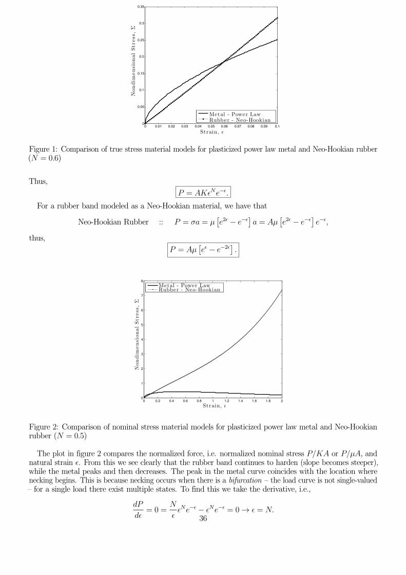
0 0.01 0.02 0.03 0.04 0.05 0.06 0.07 0.08 0.09 0.10

0.05

0.1

0.15

0.2

0.25

0.3

0.35

Strain, !Nondim

ensionalStress,!

Metal - Power LawRubber - Neo-Hookian

Figure 1: Comparison of true stress material models for plasticized power law metal and Neo-Hookian rubber(N = 0.6)

Thus,

P = AKεNe−ε.

For a rubber band modeled as a Neo-Hookian material, we have that

Neo-Hookian Rubber :: P = σa = µ[e2ε − e−ε

]a = Aµ

[e2ε − e−ε

]e−ε,

thus,

P = Aµ[eε − e−2ε

].

0 0.2 0.4 0.6 0.8 1 1.2 1.4 1.6 1.8 20

1

2

3

4

5

6

7

8

Strain, ǫ

Nondim

ensionalStress,Σ

Metal - Power LawRubber - Neo-Hookian

Figure 2: Comparison of nominal stress material models for plasticized power law metal and Neo-Hookianrubber (N = 0.5)

The plot in figure 2 compares the normalized force, i.e. normalized nominal stress P/KA or P/µA, andnatural strain ε. From this we see clearly that the rubber band continues to harden (slope becomes steeper),while the metal peaks and then decreases. The peak in the metal curve coincides with the location wherenecking begins. This is because necking occurs when there is a bifurcation – the load curve is not single-valued– for a single load there exist multiple states. To find this we take the derivative, i.e.,

dP

dε= 0 =

N

εεNe−ε − εNe−ε = 0→ ε = N.

36

Now we consider the problem for the stretch of a spherical party balloon. Considering equal biaxial stressand an incompressible rubber material that we will model as Neo-Hookian, we have that

HR2 = hr2,

where H is the thickness of the rubber in the reference state (h is the same but in the current state); Ris the radius in the current state, while r is in the reference. The Neo-Hookian model gives the true stressand stretch relationship of

σ = µ(λ21 − λ23

).

Due to the biaxial stress we have that

σ1 = σ2 = σ and σ3 = 0.

From incompressibility and the definition of the stretch we have

λ1 = λ2 = λ =r

Rand λ3 =

1

λ2.

This gives a true stress and stretch relation of

σ = µ(λ2 − λ−4

).

The internal pressure, p supplied to the balloon is what stretches it out and and from force balance in thecurrent state we have that

2πrhσ = πr2p.

From the incompressibility relation we have that

h = Hλ−2,

and using the material model, we arrive at

p =2h

rµλ−4

(λ6 − 1

)=

2H

Rµλ−7

(λ6 − 1

).

The critical radius is found as

dp

dλ=

2H

Rµ[−7λ−8

(λ6 − 1

)+ 6λ−2

]= 0 −→ λ6 − 1 =

6

7λ6 −→ λ = 7

16 .

Thus, the peak is reached at

r = 716R.

Another example of large deformation is cavitation. For plasticly deforming solids, like power law metal,a small cavity of radius A grow under internal pressure to a. For a Neo-Hookian model there is a maximum,where the size of the cavity levels off. The critical load is 5µ/2. The rest of the lecture we described theresults from Ashby (1989) where he describes hydrostatically tensioning lead inside a glass tube. He estimatesa cavity growth of three orders of magnitude.

37

Documents

Solid Mechanics Lecture Notes - Harvard John A. Paulson ...people.seas.harvard.edu/~colinrmeyer/Solid Mechanics Notes.pdf · Solid Mechanics Lecture Notes Colin Meyer Contents 1 Lecture