Embed Size (px)
Citation preview

University of Calgary
PRISM: University of Calgary's Digital Repository
Graduate Studies Legacy Theses
1999
Solution-gas drive in heavy oil: Gas mobility and
kinetics of bubble growth
Kumar, Rajneesh
Kumar, R. (1999). Solution-gas drive in heavy oil: Gas mobility and kinetics of bubble growth
(Unpublished master's thesis). University of Calgary, Calgary, AB. doi:10.11575/PRISM/17900
http://hdl.handle.net/1880/25130
master thesis
University of Calgary graduate students retain copyright ownership and moral rights for their
thesis. You may use this material in any way that is permitted by the Copyright Act or through
licensing that has been assigned to the document. For uses that are not allowable under
copyright legislation or licensing, you are required to seek permission.
Downloaded from PRISM: https://prism.ucalgary.ca

So1ution-GM Drive in Heavy Oil - Gas Mobility and Kinetics of Bubble
Orowth
by
Rajneesh Kumar
A THESIS
SUBMITTED TO THE FACULTY OF GRADUATE STUDIES IN PARTIAL
FULFILLMENT OF THE REQUIREMENTS FOR THE DEGREE OF
MASTER OF SCIENCE IN CHEMICAL ENGIHEERING
Department of Chemical and Petroleum Enginee*g
Calgary, Alberta
December, 1999

National Library 191 ,,nab Bibliothi?que nationale du Canada
Acquisitions and Acquisitions et Bibliographic Services services bibliographiques
395 Wellington Street 395, rue Wellington OttawaON KtAON4 Ottawa ON K I A O N 4 Canada Canada
The author has granted a non- exclusive licence allowing the National Library of Canada to reproduce, loan, distribute or sell copies of this thesis in microform, paper or electronic formats.
L'auteur a accorde une licence non exclusive permettaut a la Bbliotheque nationale du Canada de reproduire, prster, distriibuer ou vendre des copies de cette these sous la forme de rnicrofiche/film, de reproduction sur papier ou sur format electronique.
The author retains ownership of the L'auteur conserve la propriete du copyright in this thesis. Neither the droit d'auteur qui protege cette these. thesis nor substantial extracts fiom it Ni la these ni des extraits substantiels may be printed or otherwise de celle-ci ne doivent Stre imprimes reproduced without the author's ou autrement reproduits sans son permission. autorisation.

Abstract
Some of the heavy oil reservoirs in Canada and Venezuela under
solution-gas drive show anomalous behaviour, when compared to conventional
light oil reservoirs. Once below the bubble point pressure, producing GOR does
not increase sharply and rate of pressure drop is low. Some wells show higher
oil production rates than those predicted using conventional flow equations in
radial coordinate. The overall recovery under solution-gas drive is higher than
that expected from a simitar conventional oil reservoir.
Research was initiated to study solution-gas drive in heavy oil reservoirs.
and investigate the reasons for the favourable behaviour. In the first part of the
research program, gas phase growth was studied by modelling bubble growth in
bulk and comparing growth in light and heavy oil. The effect of step and
gradual change in pressure was studied. Further, a model was developed to
study gas phase growth, in a closed system, for constant volumetric rate
depletion. Sensitivity of various parameters on behaviour of the system was
studied. One of the hdings of the study was that, the pressure in the system
can fall even after generation of bubbles in the system. Thus, the bubble
nucleation need not coincide with the minimum point on the P-V cume (known
as "Critical Supersaturation"). A new term "Apparent Critical Supersaturation"
was coined to represent minimum point on the P-V curve.
In the second part of the project, flow experiments were performed to
measure the mobility of gas in heavy oil. Depletion was performed at various
rates to study the effect of depletion rate on critical gas saturation and
supersaturation. The experimental data was matched on Eclipse-100 black oil
simulator to determine the gas relative permeability at various depletion rates.
Results indicate that the gas relative permeability under solution-gas
drive in heavy oil is very low. This is attributed as one of the factors leading to
favourable behaviour of heavy oil resemoirs.

Acknowledgement
This work was a result of continued support, guidance, encouragement,
understanding and patience of many individuals and organisations. Although
the efforts have been priceless, I would like to gratefully thank all of them for
their contributions,
First of all, I would like to thank my s u p e ~ s o r , Dr. Mehran Pooladi-
Darvish, for providing me an opportunity to pursue a Masters degree. His
knowledge of the project and enthusiasm was infectious. He was always polite,
encouraging and accessible any time of the day for fkuitful discussions. He
provided me opportunity to perform independence research; nonetheless being
always there when I needed him. I also thank him for all the non-project
related discussions we had, I was fortunate to have such an understanding
supervisor and I can say that in this process I found a nice friend.
The experiments were carried out at the Imperial Oil Research Centre in
Calgary. I consider myself fortunate enough to be associated with such an
organisation and would cherish the memories I had here. I would like to thank
Dr. Tadahiro Okazawa for providing guidance, support and valuable
suggestions for this work.
I wish to acknowledge Ms. Kathleen Corry for her incessant efforts in
making the experiments a success. I thank her for all the invaluable help and
advice she offered in setting up the experiment. She was extremely
instrumental in steering the project thorough, in some of the most difEcuIt
phases. I would also like to thank Mr. Brad Harkar for his technical expertise,
and always coming out with some brilIiant ideas in case of dire need. I also
wish to acknowledge Mr. Mike Ruckdaeschel and Mr. Doug Rancier for their
help in setting up the experiments.
I would like to thank Dr. Roland Leaute and Dr. Rick Kry for some
insigh- comments. Further, I would like to acknowledge the staff at Imperial
Oil for their support during my stay and running the experiments.

I would also like to thank my committee members Dr. B. B. Maini and
Dr. R. C. K. Wong for taking out time to read my thesis. They are undoubtedly
among one of the most prollic and knowledgeable persons in this area. I
consider myself fortunate enough to have them on my defence committee. I
would like to thank Dr. B. B. Maini for his valuable advice during the
experiments.
1 would like to thank my wife, for understanding my desire to pursue
higher studies. She has been extremely supportive and patient and has
contributed in ways I would always appreciate. I would like to thank my
parents, for their love, upbringing and sacrifice, and making me the person I
am today.
In the end, I would Iike to thank the Natural Science Engineering and
Research Council (NSERC), Alberta Department of Energy (ADOE) and Imperial
Oil for providing h d i n g for the project. I would also like to thank the
Department of Chemical and Petroleum Engineering and all the fellow graduate
students for their help during m y studies at the university.

To,
my patents
From the unreal lead me to the real I From darkness lead m e to light !
From death lead m e to immortaIity I
Title page ............................................................................................... Approval page ....................................................................................... Abstract ..............~................................................................................... Acknowledgement ................................................................................... Dedication .............................................................................................. Table of contents .................................................................................... List of tables ........................................................................................... List of figures ........................................................................................
Nomenclature .........................................................................................
V1
vii
xi
xii
xiv
CHAPTER ONE: INTRODUCTION
1.1 Background .......................................................................... 1
1 . 2 Layout .................................................................................... 2
CHAPTER TWO: LITERATURE REVIEW
2.1 What is solution-gas drive? ....................................................... 3
2.1.1 Supersaturation ................... ... ...................................... 4
2.1.2 Nucleation ...................~................................................... 5
2.1.3 Bubble growth ................................................................... 8
.......................*....*... .. . 2.1.4 Coalescence ..... ., 11
....................................................... 2.1.5 Critical gas saturation 12
2.1.6 Gasflow ........................................................................... 14
2.2 Anomdous behaviour of heavy oil reservoirs ............................... 16
......................................................................... 2.3 Models proposed 18
2.3.1 Presence of microbubbles ................... ... ........................ 18
.....................*...*....... .......**.*....*..* 2.3.2 Lowering of viscosity .. 19
2.3.3 Foamy oilflow ................................................................... 20
2.3.4 Pseudo-bubble point model ................................................. 23
2.3.5 High n i t i d gas saturation .............................................. 23
vii

2.3.6 Geo-mechanicul effects .......................... .. ....................... 2 5
2.3.7 Increased oil mobility .......................................................... 26
2.3.8 Lower gas mobility ............................................................. 27
2 . 4 Relative permeability .................... .... ...................................... 28
2.4.1 Introduction ........................................................................ 28
2.4.2 Measurement of relative permeability ................................... 29
2.4.3 Relative pemeabilit y under solutiongas drive ................... ... 32
2.4.4 Discussion ........................................................................... 34
2.4.5 Selection of experimental method .......................................... 36
CHAPTER THREE: OBJECTIVE
3.1 Scope of the study .......................... ... ......................................... 38 3.1.1 Kineticsofbubblepwth ........ ... ....................................... 38 3.1.2 Gas mobility measurement .................................................... 39
CHAPTER FOUR: KINE3ICS OF BUBBLE GROWTH
.................................................................................... 4.1 Introduction 41
4.2 Statement of the problem ................................................................ 42
4.2.1 Hydmd ynamic growth model .................... ... .. ... ............ 43
4.2.2 Diwonal growth model ..................... ... ........................... 44
4.2.3 General growth model ............................................................ 45
4.2.4 Dimensionless fornutation ...................~.~~.~~.~~.....~....~............. 46
4.2.5 Gmdual decline in pressure model ......................................... 48
4.2.6 Finite domain model ............................................................. 49
...................................... 4.2.7 Modelling solution-gczs drive process 50
4.2.8 Physicatparametersused insimulation ................................. 51 4.3 Results ........................................................................................... 52
................................................... 4.3.1 Gradual decline in pressure 52
............................................ 4.3. 1.1 Infinite domain results 52
4.3.1.2 Effectofno-flowboundary ...................................... 61
4.3.2 Grrs phase build-up during solution-gas drive ..................... .... 63

4.3.2.1 Results .................................................................. 64
4.3.2.2 Se-tivity studies ................... .. ...... ..... ............. 70 4.3.2.2.1. Efect of depletion rate ................................ 70
4.3.2.2.2. Effect ofviscosity ............................ ... .... 75 4.3.2.2.3. Erect of d i m o n coeflcient ........................ 75
4.4 Discussion ....................................................................................... 76 4.5 One possible scenario for bubble generation .................................... 77
.............................................. 4.6 Conclusions ,.. . 78
CHAPTER FIVE: GAS MOBILITY MEASUREMENT
...............,............... ..*........,........................................ 5.1 Introduction .. 80
5.2 Experimentai setup .......................................................................... 81
5.3 Fluid data ........................................................................................ 84
5.4 Experimental procedure ................................................................... 85
5.5 Running experiments ....................................................................... 102
5.5.1 Depletion runs ................... .. ..................................................... 102
5.5.2 Reduction measurement ............................................................. 103
5.6 Results ............................................................................................. 103
5.6.1 Pressure ................................................................................. 104
5.6.2 Differentialpressure ................................................................... 106
5.6.3 Average gas saturation and production .................. ... ........... 113 .................................. ...................... 5 -7 Analysis and Discussion .... 116
5.7.1 Simulation ofthe experiments .............................................. 116
5.7.2 Analysis ofthe results ............................................................ 118
5.7.3 Discussion ............................................................................. 127
5.8 Conclusions ..................................................................................... 127
CHAPTER SIX: SUMMARY AND RECOMMENDATIONS
6.1 Summary ......................................................................................... 129
6.2 Recommendations ........................................................................... 130

..... REFERENCES ................... ... ...................... .... 132
. APPENDIX I: Solution for bubble growth ............................................... 145
. APPENDIX 11: Algorithm for solution ...................................................... 162

LIST OF TABLES
Table Dercription page
Dimensionless parameters ................... .. .................................. Parameters used in simulation of bubble growth ...................... .... Parameter used in simulating experimental data of
Pooladi-Darvish and Firoozabadi (1999) ....................................... ... ..........*.......-....*.......*....*. ....................... Roperty of fluid .. ..
Property of sand-pack .................................................................. Experimental data for measurement of dead oil viscosity .............. Summary of results ..................................................................... Data used in simulation of experiments .......................................

LIST OF FIGURES
Schematic representation of the problem ........................LC......... 43
Representation of bubble growing in h i t e domain .................... .. 49
Diffusion limited vs . general gowtir
gradual decline in pressure ................... .. .. .. ........................ 53
Comparison of bubble growth for gradual dedine
in pressure (100 psi./ hr.) for various cases .................. .... ......... 55
Comparison of bubble growth: step change vs . ...................... ....................... gradual change in pressure .... 56
.................... .....*.*... Effect of depletion rate on bubble growth ... 58
Constant 'a' for growth model ...................................................... 59
Effect of initial bubble radius on bubble growth ........................... 60
.......................... NO-flow boundary vs . infinite boundary solution 62
Comparison of model with experimental resuits ....................... .... 65
................................ Effect of depletion rate on system pressure 68
Effect of depletion rate on bubble radius ................ ...... .......... 69 .......................................... Effect of viscosity on system pressure 71
.............................................. EEect of viscosity on bubble radius 72
Effect of diffusion coefficient on system pressure .......................... 73
............................................ Effect on diffusion on bubble radius 74
...................................................................... Experimental setup 82 .................................................................................. Core-holder 83
....................................... Visual cell (Gas-Oil separator) ... .. . .. .... .... 83
.................................................................. Sand extraction setup 88
...................................... Viton sleeve with multiple pressure taps 88
Determination of absolute permeability ........................................ 93 Determination of effective permeability ......................................... 93
............................................................. Haake PK- 100 viscometer 95
xii

Viscosity vs . temperature for dead oil ........................................... 96
P-V graph for determination of dead oil compressibility ................ 98
Determination of compressibility of live oil ................................. 98
CompressibiIi~~ determination of sand-pack .........................-....ti. 99
Setup for measurement of gas-oil ratio .................... ... ...... .. ... 99
Setup for solution gas-oil ratio (R.0) measurement .................... .. 101
Measured solution gas-oil ratio .................... .. ........................ 101
Average pressure vs . depletion: experimental and
simulated data . .............................................. ............................. 105
Differential pressure for Run 1 .................................................... 107
Differential pressures for Run 3, 4 and 6 ................................... .. 108
Experimental production-end and no-flow boundary
pressures (Run 4) .........~.............................................................. 110
System and differential pressure: 3cc/hr (Run 4) ..................... .... 111
Gas saturation-experimental vs . simulated data .......................... 114
Produced gas-Experimental vs . simulated results ........................ 115
Pressure results for R u n 4 (Simulated results) ............................. 119
Gas relative permeability ............................................................. 121
Critical gas saturation vs . depletion rate ...................................... 122
End point value vs . depletion rate ................................................ 123 Apparent critical supersaturation vs . depletion rate ..................... 124
Gas relative permeability for O.OBcc/hr ........................................ 126
A l Schematic representation of the bubble growth system ................ 145
A2 Schematic of the numerical solution scheme ................................ 161
xiii

NOMENCLATURE
area, m2
bubbles
rate of pressure drop, Pa/ s
mass concentration, kg/m3
diameter, m
diffusion coefficient, m2/ s
friction factor
dimensionless pressure parameter
jacob number
Henry's constant, Pa./Kg/mJ
permeability, m2
length, rn
molecular weight, Kg/KMol
fluid pressure, Pa.
pressure drop, Pa.
flow rate, m3/s
radial coordinate
bubble radius, m
temperature. OK
reynoIds number
solution gas-oil ratio, m3/ ma
supersaturation, Pa.
saturation
schmidt number
time coordinate
velocity, m/s
voiume, m3
kee energy
empirical constant

2 = gas compressibility factor
B - formation volume factor, nn3 / m3
Subscripts
viscosity, P a s
dimensionless time
dimensionless radius
dimensionless pressure
dimensionless radial coordinate
dimensionless surface tension parameter
bokzmann's constant
density, kg/&
kinematic viscosity, m/ s2
surface tension, N/m
gas constant, Pa. m3/KMol. OK.
compressibility, Pa-1
error in guess value of concentration in simulation
error in guess value of radius in simulation
initial value
at the first grid point i.e. at the interface
capillary
dead oil
effective
estimated value
final value
formation
gas
position in space grid
initial (at bubble point)
previous value

Superscript
liqyid
number
oil
value at residual oil saturation
pore value
at bubble interface
relative value
standard conditions
total
at the interface
value at far away point
0 - - end point value * - - dimensioniess value
n - - time step number -
rbr - corey's exponent

Chapter 1
INTRODUCTION
1.1. Background
As the conventional light oil resources diminish, need to develop the
heavier oil resources draws more attention, The total estimated resource of
heavy oil and bitumen in the world is about 5 trillion barrels, of which Canada
holds about 2.7 trillion barrels Putler, (1991)l. The heavy oil, having a higher
viscosity, does not flow out of the reservoir as readily as conventional light oil.
This had initially been sighted as an unfavourable attribute, predicted to result
in lower primary recovey based on application of conventional flow equations
in radial geometry,
In some parts of Western Canada and Venezuela, anomalously high
recovery of heavy oil under solution-gas drive was reported, thus contradicting
the prediction using the conventional methods. This was accompanied by lower
gas-oil ratio and pressure maintenance in the reservoirs. The heavy oil
production in some areas in Canada has been accompanied by high sand cuts.
A new term "Cold Production" was coined to represent such process. In mid
80's Smith (1988) pioneered the research on heavy oil recovery under solution-
gas drive and brought this favourable behaviour of heavy oil reservoirs to the
attention of the oiI industry. His paper triggered off research in this fidd.
Following his paper, various research projects were initiated; aiming to have a
better understanding of the process and generating a model that could explain
this behaviour of heavy oil systems. The model thus generated was intended to
be used to predict performance of the reservoir and also to efficiently manage
and produce the reservoir.
The high viscosity of heavy oil results in unfavourable mobility ratio
during water flood, leading to low sweep efficiency and poor oil recovery. Thus

2 more expemsive thermal methods have to be applied for higher recovery of heavy
crude oils. The favourable behaviour of heavy oil resemoirs under solution-gas
drive is an encouraging feature for the oil patch in Canada, where heavy oil
makes up a larger portion of total oil produced year after year [AEUB (1997)l.
With better understanding and proper modelling of solution-gas drive in heavy
oiI, higher initial oil recovery can be achieved at much lower cost. Further, the
reservoir can be optimally produced in such a way that subsequent application
of thermal processes are more effective. Efficient primary production has more
significance to some of the thin reservoirs in Canada where a lot of heat is lost,
to the under and over lying formations, should thermal processes such as cyclic
steam stimulation (CSS) and steam drive be used.
This research is in continuation of the efforts being made to have a better
grasp of the cardinal principles underlying the solution-gas drive process in
heavy oil. Theoretical and experimental techniques are employed. Modelling
efforts concentrate on more fundamental aspects of the process. Experiments
have been designed such that conclusions can be drawn regarding the process
under field conditions. Comparisons have been made with the rapidly
expanding body of the literature on the subject.
1.2. Layout
The thesis starts with literature review (chapter 2) with specific
application to solution-gas drive process in heavy oil. This is done keeping in
view the anomalies observed in heavy oil reservoirs and various works done on
that. Following literature review the objectives of the thesis are stated in
chapter 3. Chapter 4 presents the bubble growth model developed for ~01ution-
gas drive process. In chapter 5, experimental work on gas mobility
measurement is presented and results discussed. Chapter 6 concludes the
study with summary and recommendation for hture work.

Chapter 2
LITERATWRE REVIEW
2.1. WEat h Solution-gas drive?
When the pressure of an originally undersaturated reservoir is lowered
below the bubble point, the gas phase is generated. The gas phase, being
compressible, helps maintaining the pressure in the reservoir and hence
provides the driving force for primary production. The gas does not flow as an
independent phase until it reaches certain saturation known as the Critical Gas
Saturation After this, the gas flows as an independent phase. Since, the gas
mobility is significantly greater than that of oil, the gas production rate is much
higher than that of oil. Conventionally, this results in a high producing GOR
(Gas-Oil Ratio). The high gas production rate results in rapid dedine in
reservoir pressure. This mode of primary recovery is known as the Solution-gas
drive. The process of solution-gas drive involves supersaturation, which results
in nudeation of the gas bubbles, followed by bubble growth and coalescence
and hnally flow of gas as an independent phase.
Sections (2.1.1-2.1.6) present the literature review on the various steps
involved in solution-gas drive process, with specific application to solution-gas
drive in heavy oil. Next, the anomalous behaviow of heavy oil reservoirs is
stated (2.2). This is followed by a brief review of the various models proposed to
explain this behaviour (2.3). One of the aims of the study is to measure gas
relative permeability under solution-gas drive in heavy oil. A brief review on
relative permeability is presented in section 2.4. This indudes introduction,
various methods for measurement of relative permeability, relative permeability
measurement under solution-gas drive process, discussion and selection of

experimental method for measuring the relative permeability under solution-gas
drive.
2.1. I. Supersaturation
When the pressure is lowered below bubble point in an undersaturated
reservoir, gas bubbles are expected to be generated as per the equilibrium PVT
properties. A certain supersaturation is required for nucleation of bubbles. So,
the pressure in the system f d s below bubble point without generation of gas
phase. The system in this state, is said to be supersaturated.
Supersaturation can be defined as the difference between actual oil
pressure and the saturation pressure corresponding to the amount of gas
dissolved in the oil [Kamath and Boyer (1995)l. The system may remain
supersaturated even after nucleation has taken place, for various reasons.
Kennedy and Olson (1952) observed supersaturation as high as 770 psi
(5307 KPa), during fast depletion rates on methane in kerosene solution, before
nucleation was detected. At supersaturation of 30 psi (207 KPa) no bubble was
found to nucleate, even when the liquid was kept for 138 hours. They found
that supersaturation affected the nucleation rate, and evaluated a function for
nucleation rate as a h c t i o n of supersaturation.
Various fmors have been reported to affect supersaturation. Resence of
asphdtenes has been reported to increase supersaturation [Bora and Maini
(1997)l. Bora and Maini (1997, carrying out pressure depletion test in glass
micromodel found out that higher oiI viscosity gives higher supersaturation.
Higher depletion rates resulting in higher supersaturation has been
reported by several researchers [Stewart et aL (1954), Dumore (19701, M O ~ U
(1989), Wall and Khurana (1972), Hunt and Berry (195611. Hunt and Berry
(1956) reported a supersaturation of 10 psi (69 KPa) after carrying out depletion
experiments for 40 days, even though the depletion rate was extremely low (1
psi/day (6.9 KPafday)) and gas bubbles were generated on the 20* day. Recent
experimentai results [Pooladi-Danrish and Fioozabadi (1999), Guo-Quig and

Firoozabadi (1999)], at comparatively higher depletion rate, indicate no
supersaturation, after certain time (20-30 days) following nucleation of bubbles.
The degree of supersaturation was related to pore structure by
Firoozabadi et a1 (1992). They conducted constant volumetric rate depletion
experiments on two Merent types of rock samples and concluded that smaller
grain size may lead to lower supersaturation.
Supersaturation is a driving force for nucleation and bubble growth and
is afEected by various parameters. The intricate influence of these variables and
supersaturation on solution-gas drive is an area of further research.
2.1.2. Nucleation
Cavitation and boiling are the two ways in which bubble formation can
occur in liquid phase. The formation of gas bubble due to lowering of pressure,
at constant temperature, below bubble point is known as cavitation. O n the
other hand, boiling involves raising the temperature above boiling point, at
constant pressure. Cavitation is the nucleation mechanism taking place in
resenroir under solution-gas drive and shall be discussed here.
In a recent study, Jones et at. (1999) presented a novel classification for
nucleation:
1. classical homogeneous nucleation
2. classical heterogeneous nudeation
3. pseudo classical nucleation
4. non-classical nudeation
In classical homogeneous nucleation the bubbles are generated in the
bulk. Nucleation starts by formation of embryo, which grow to nuclei and then
to bubbles. Very high supersaturation is required m this class of nucleation
[Hemmingsen (1975)l. For homogeneous nucleation, the expression for rate of
nucleation, was given by Brennen (1995) as:

where Z is the total number of gas molecules present in the system, W is
the driving free energy needed to aeate a duster, y/ is BoltPnann's constant, T
is the temperature in Kelvin, o is the interfacial tension and s is the
supersaturation. The critical radius formed is given by:
The above equation implies that, higher supersaturation leads to
formation of smaller bubbles.
The classical heterogeneous nucleation is catalysed by presence of
impurities or rough surface. The surface energy is lowered, that in tun lowers
the supersaturation required for nucleation. In heterogeneous nucleation the
bubbles nucleate on foreign particles, thus the work done to aeate a bubble is
several orders of magnitude less than that required for homogeneous
nudeation. Heterogeneous nucleation has been suggested as one of the more
probable mechanisms taking place in porous medium [Firoozabadi et al.
(1992)J. The nucleation rate expression for heterogeneous nucleation is given
by Moulu ( 1989) as
The values for constants Z and A were experimentally determined, for
crude oil system in porous media p o u l u (1989)j. The equation is written as
The last two classiiications involve presence of pre-existing bubbles. In
pseudo classical nudeation the pre-existing bubble radii are smaller than the
critical radius and have to overcome capillary barrier to grow, whereas, in non-
classical nucleation, the bubbles radius is larger than the critical radius and all
of them grow since there is no activation energy reqyired.
The other dassiflcation of nudeation, is reIated to the duration of
nucleation. NucIeation can be divided into two categories, which are
a) instantaneous nucleation

b) progressive nucleation
Instantaneous nucleation theory states that all the bubbles are
nucleated at a single value of supersaturation. No further nucleation of
bubbles takes place as the depletion proceeds. Whereas, in progressive
nucleation, the bubbles nucleate at all values of supersaturation, as depletion
progresses. The debate, that the nudeation in porous medium during
cavitation is instantaneous or progressive, has been going on for a long time
now. Kashchiw and Firoozabadi (1993) proposed instantaneous nucleation to
be taking place in the reservoir. Geilikman et al. (1995) said that majority of
the bubbles nucleate at maximum supersaturation. He defined this process as
"expiosive foaming or bubbling". Bora and Maini (1997) observed nucleation of
bubbles even after other bubbles had nucleated. They thus conduded that
nucleation in porous media is not instantaneous but progressive.
Bora and Maini (1997) observed two types of nucleation processes. In
the first type, the nudeation site became inactive after generating bubble. This
could be due to trapped gas, which is a non-classical type of nucleation. In the
second type, the site produced a string of bubbles. This could be due to
capillary pressure criteria being met at the crevice. The impurities were
observed to assist nucleation. They also observed that nucleation mostly
occurred at pore w d s . However, asphaltenes were not found to assist
nucleation. Danesh d aL (1987) stated that the presence of connate water can
delay the formation of vapour phase. Bora and Maini (1997) also reported
similar results. However, Kenncdy and Olson (1952) observed no effect of water
on fkequency of bubble formation. Kamath and Boyer (1995) mentioned that
nudeation might be facilitated due to presence of connate water.
Hunt and Berry (1956) realised the discrepancy observed in pressure
data, for nucleation of first bubble, when similar experiments are carried out,
for reproducibility of results. They presented a probability function to exp1ai.n
this discrepancy. They also presented results for number of bubbles formed at
various pressure decline rate and stated that the number of bubbles nudeated
innease with increase in pressure dedine rate. The oil recovery has been

reported [Stewart et aL (1954)l to depend on the number of bubbles fonned
during the solution-gas drive process. Several other researchers [Danesh et ale
(1987, M o u l u (1989), Bora and Maini (19971, Wall and Khurana (1972)j have
also reported that faster depletion rate leads to nucleation of more bubbles.
Kennedy and Olson (1952) quantiiied this and presented values for bubble
density at different depletion rates. They said that one bubble is formed in
every million pore even at very high depletion rates. They also concluded that
the nucleation rate was a function of supersaturation only, and evaluated a
bc t ion for nucleation rate as a function of supersaturation. Comparing
nudeation on calcite and silica, they concluded that both are equally effective
in promoting formation of bubbles.
Wong et al. (1999) concluded that the number of bubbles formed is not
af5ected by fluid viscosity. Considering that, diffusion coefficient is a function of
oil viscosity, the lower diffusion coefficient may lead to generation of more
number of bubbles. Pooladi-Darvish and Firoozabadi (1999) and later on Guo-
Quig and Firoozabadi (1999) reported more number of bubbles, when
conducting experiments with heavier oil as compared to that observed when
using lighter oil. Similar results have been reported elsewhere [Bora and Maini
(1997), Main i (1999)l.
There seems to be several different dassifications for bubble nucleation.
The nucleation appears to be a strong function of the mode and conditions
under which experiment is carried out. Minute variation in experimental
process and condition can lead to different results. Experiments should be
carried out carefully and under exactly similar conditions to achieve
satisfactory duplicate results.
2.1.3. Bubble growth
Once the bubbles nucleate, they start growing. The rate of growth of
bubble determines the gas phase growth in porous media, and hence is of
partidar interest for soIution-gas drive process.

It has been reported [Scriven ( 19591, Szekely and Martins (197 I), Szekely
and Fang (1973). Rosner and Epstein (1972), Patel (1980)I that a number of
parameters viz. viscosity, surface tension, diffusivity and initial bubble radius
play a significant role in determining the rate of growth of a bubble. The forces
that govern the growth of a bubble can be broadly classified into two categories.
One being the hydrodynamic (inertial, pressure and viscous) forces and the
other being the diffusional force. The inertial, pressure and the diffusional
forces are the forces assisting growth, whereas the viscous forces resist growth.
This problem has been extensively studied in the chemical engineering
literature, especially when the process is dominated by one of the forces, only.
Scriven (1959) simplified the bubble growth problem by neglecting the
hydrodynamic forces and presented an analytical solution for the diffusional
growth problem for a particular range of mass transfer driving force. Later on,
the effect of other parameters was included by others [Szekely and Martins
(197 13, Szekely and Fang (1973), Rosner and Epstein (1972), PateI (1980), Li
and Yortsos (1995)l. Rosner and Epstein (1972), Pate1 (1980) and Szekely and
Martins (1971) concluded that at early times of bubble growth in a bulk liquid,
the inertial forces limit bubble growth, but at later times it is limited by
difFusional forces. Szekely and Martins (1971) and Patel (1980) showed &at
increase in viscous forces lead to lower rate of bubble growth at early time.
The above bubble growth studies in bulk considered the case when the
pressure was dropped in a step. The bubble growth for gradual decline in
pressure is of particular interest, since it more closely simulates reservoir
conditions.
Kashchiev and Firoozabadi (1993) reviewed many of the limiting models
when either hydrodynamic forces or mass transfer forces dominate bubbIe
growth. It was shown that in some cases, bubble growth can be modelled by
R(t) = atb, where R and t are bubble radius and time, and a and b are constants.
Danesh et aL (1987) carried out depletion experiments in glass
micromodel and observed that the growth of bubbIes m porous media was
controlled by capi l la~~ force. They observed no effect of gravity and direction of

flow on the pattern of growth. However, later on, contradicting their earlier
statement, they said that gas may not always occupy the largest pores and
leave oil behind in tighter pores. They observed gas entering and displacing oil
in tight pores instead of entering the larger pores.
The approach, to model gas phase growth in porous media should
incorporate capillary pressure terms. Moulu (1989) and Hunt and Berry (1956)
neglected the hydrodynamic and capillary forces in treatment of the bubble
growth problem in porous media. Moulu (1989) developed a comprehensive
theoretical model for heterogeneous bubble nucleation, followed by growth and
then attainment of critical gas saturation. He was successful in matching the
experimental results quiet well, even while neglecting capillary forces. However,
looking at the diffusion growth equation, it seems he neglected the moving
boundary term, caused by the expansion of bubble. His model has been used
by other researchers [Sheng et a[. (1999)], while modelling solution-gas drive
process in porous media.
Hunt and Berry (1956) presented an analytical solution for the
diffusional growth equation for a set of initial and boundary condition. However
it is not dear in their analysis how the pressure at the far boundary is
changing.
Li and Yortsos (1995) presented a detailed theoretical network model for
multiple bubble growth in porous media including the terms for capillary forces.
They presented several scenarios for bubble growth and criticat gas saturation.
Modelling solution-gas drive process, Firoozabadi and Kashchiev (1996),
assumed instantaneous nucleation to take place at maximum supersaturation.
They used the a t b model for growth and were able to match experimental data of
gas phase growth during the solution-gas drive process. They considered
nudeation to occur at the lowest point on the P-V curve.
Bubble growth is one of the key parameter in modelling solution-gas
drive. The forces governing the growth need to be delineated and properly
accounted for while modelling the growth. Further, the applicability and
validity of the emp i r i d growth models need to be ascertained before usage-

2.1.4 Coalescence
Coalescence occurs when the two bubbles come close to each other. This
is followed by thinning of liquid lamella separating the bubbles which involves
flow &om between the bubble surfaces towards its periphery. Coalescence, has
been reported to be afTected by a number of factors, including bubble size,
Liquid property, porous media etc.
Gedhnan et aL (1995), in their analysis showed that small bubbles tum
out to be strongly compressed by capillary forces and do not coalesce. This,
they said, is because there is no gain in surface energy due to coalescence.
Whereas the larger bubbles, coalesce rapidly, as coalescence leads to reduction
in surface energy. As stated eariier, higher supersaturation, which is due to
faster depletion rate, leads to smaller bubbles. Hence, higher depletion rate
leads to formation of smaller and more stable bubbles,
Coalescence was reported to happen more readily in light oil than in
heavy oil, in experimental results of Pooladi-Darvish and Firoozabadi (1999).
This might be an indication of effect of viscous forces on coalescence.
Dusseauit (1993) stated that the bubbles formed in heavy oil do not readily
coalesce due to high viscosity of oil and capillary forces. Studies have shown
that presence of asphaltenes hinders coalescence and stabilizes the gas bubbles
[Bora and Maini (1997)]. From their pressure depletion tests in glass
micromodel, Bora and Maini (1997) also concluded that coalescence is more
likely to occur at low liquid velocity (lower depletion rate).
Islam and Chakma (1990) stated that there is distinct impact of presence
of asphaltenes on gas bearing capacity of oil. They showed that the entrained
gas content of oil increases with increase in asphaltene content. This can be
due to formation of more stable bubbles that lead to dispersed gas flow.
Pooladi-Darvish and Fimozabadi (1999) and Guo-Quig and Firoozabadi (1999)
reported that the bubbles do not remain isolated in heavy oil in porous media,
but coaIesce to form a bigger gas phase before flowing.

Ward et al. (1982) and Ward and Levart (1984) showed that small
bubbles can be stable due to presence of impurities. Ward et a2. (1982) also
showed that increase in number of bubbles in closed volume reduces the size of
the bubble required for equilibrium. Thus it can be inferred that presence of
asphaltene in a resenroir can lead to smder and more stable bubbles.
The presence of porous media on stability of bubbles has been discussed
in detail by Kovscek and Radke (1994). They stated that in the bulk, the larger
bubbles grow at the expense of smaller bubbles. This is because the bubble
size and radius of curvature are directly proportional to each other. However,
in porous media, lamella curvature depends on pore dimension and location
within pore space. They concluded that, in porous media, coalescence happens
only when the lamella reaches the same pore throat.
Coalescence is a complex process and one that is not well understood
and modelled. I t is of importance because it determines the number of lamella
and gas saturation morphology in porous media. This in effect is a measure of
the resistance to gas fI ow and hence a factor affecting gas relative pemeabiliw.
2.1.5 Critical gas saturation
The gas phase under solution-gas drive is not mobile at low saturations.
As the depletion progresses, the gas phase grows due to W s i o n , pressure
reduction and coalescence. A certain saturation of gas is required before a
mobile gas phase can be realised. This gas saturation is known as critical gas
saturation. The importance of critical gas saturation stems from the fact that it
signals the onset of fkee gas flow, thus depleting the reservoir of the driving
force for primary production.
WalI and Khurana (1972) dehned critical gas saturation as minimum gas
saturation which must exist before any flow of gas may occur.
Firoozabadi et aL (1992) gave a similar definition for critical gas
saturation. A very low critical gas saturation vdue has been reported in their
work (0.5 - 1.5%). They related critic& gas saturation to supersaturation and

pore structure. They concluded that critical gas saturation decreases with
decrease in supersaturation.
Very high values of critical gas saturation have also been reported in
literature, especially for solution-gas drive in heavy oil [Loughead and
Saltuklaroglu (1992), Sarma and Maini (1992), Islam and Chakma (1990)j.
Kamath and Boyer (1995) defined critical gas saturation as minimum
saturation for continuous gas flow through porous medium. They discussed
critical gas saturation in external and internal gas drive and showed that the
values are very different in the two cases. They reported critical gas saturations
of 1 and 10% under extemal and solution-gas drive processes, respectively.
Li and Yortsos (1995) defined critical gas saturation as formation of a
sample-spanning duster. Pooladi-Darvish and Firoozabadi (1999) defined
critical gas saturation as the minimum gas saturation at which the gas flow can
be sustained. Here, in this study, we define critical gas saturation as the gas
saturation at which a sustained, though intermittent, gas flow can occur.
Numerous researchers [Hunt and Berry (1956), Firoozabadi et al. (1992),
Kamath and Boyer (1995)l have studied the effect of depletion rate on critical
gas saturation. A unanimous conclusion has been that critical gas saturation
increases with increase in depletion rate.
Li and Yortsos (1995) developed a model for multiple bubble growth in
porous media and concluded that for instantaneous nucleation w i t h constant
nucleation fkaction the critical gas saturation is independent of depletion rate.
However, the critical gas saturation was reported to increase with nudeation
fraction for case of instantaneous nucleation. Whereas, for progressive
nucleation (sequential activation), the critical gas saturation increases with
depletion rate.
Critical gas saturation is one of the factors affecting recovery under
solution-gas drive, provided other parameters remain the same. A high critical
gas saturation delays gas production and hence increases recovery. The
dependence of critical gas saturation on so many factors warrants that properly

designed experiments, simulating field conditions, be carried out to have a
reasonably accurate value.
2.1.6 Gas flow
Once critical gas saturation is reached, gas starts flowing as an
independent phase, thus depleting the reservoir of the driving force for primary
production. The gas flow can mainly be in two forms
1. dispersed gas flow
2. continuous gas flow through gas channels
The former represents low gas phase mobility whereas the gas mobility in
the later case is comparatively higher (this shall be justified later). The later
case is undesired during solution-gas drive process, since it leads to rapid loss
of gas firom the reservoir. Several microscopic and macroscopic studies have
been conducted to understand and model this part of the process, since it is
affected by so many parameters.
Bora and Maini (1997) observed that in slow depletion tests the bubbles
do not vacate the original pore and migrate towards the outlet. Thus the slow
depletion tests displayed dassical solution-gas drive behaviour. Contrary to
this, in faster depletion tests, the bubbles were obsewed to nucleate, grow and
then move towards the outlet end. In this process the bubbles would split. The
split bubbles would then grow and split again as they moved towards the outlet.
This was referred to as dispersed gas flow. They concluded that high viscosity
coupled with high velocity leads to dispersed gas flow. In earlier work, Sarma
and Maini (1992) said that the heavy oilfgas mixture flows in form of oil
continuous foam. Snap-off phenomenon was observed in solution-gas drive
experiments conducted by Danesh et al. (1987) in glass micromodel. They
reported that snap-off is promoted by higher velocity and structure of the
porous media (high pore body to pore throat ratio).
Wall and Khurana (1972) stated that during slower pressure decline, gas
flows intermittently. There is a period of gas saturation build-up during which

no gas flow occurs. This is followed by period of gas flow. SimiIar behaviour
was observed in slow depletion experiments of Pooladi-Darvish and Firoozabadi
(1999).
Wall and Khurana (1972) conducted pressure depletion experiments and
reported that increase in flow rate fiom one value to another leads to
intermittent gas flow at higher equilibrium saturation. They concluded that the
final gas saturation increases with pressure dedine rate.
Wong et al. (1999) carried out pressure depletion tests on bitumen. They
said that the gas flows through free gas channels after reaching critical gas
saturation. A constant increasing GOR (Gas-Oil Ratio) should be observed if
gas flows through channels. However, the produced GOR results indicate
fluctuating values of produced GOR. This may be due to intermittent flow of
gas, which happens when dispersed gas flow occurs in the porous media.
Dumore (1970), from solution-gas drive experiment in transparent
porous media, concluded that dispersed gas flow results in higher gas
saturation; an observation that holds true for the results of Pooladi-Darvish and
Firoozabadi (1999). He also stated that dispersed gas flow in a porous media is
a function of the pore structure of the porous media. He found a value, for
transition &om dispersed to non-dispersed flow, f?om his external gas drive
experiments. The study concluded that high capillary pressure leads to non-
dispersed flow whereas low capillary pressure leads to dispersed flow.
The modelling of gas flow is quite complex at microscopic level. At
macroscopic levels Darcy's equation is used to represent the flow. The
parameter most often changed to represent flow a t a particular gas saturation is
gas relative permeability and viscosity.
Modelling of each of the individual processes in solution-gas drive
presents a unique challenge, as it depends on so many parameters and is
affected by so many process variables. A proper comprehensive modelling
should take into account non-equilibrium phenomenon (supersaturation),
nucleation (type of nucIeation, rate etc.), growth of gas phase (induding
hydrodynamic, difiusive and capillary forces), coalescence, gas flow (dynamic
effect of change in gas saturation distribution on gas flow), effect of porous
media among other parameters.
2.2 Anomdous behaviorv of heavy oil reaerpoirs
The heavy oil reservoirs in Westem Canada and Venezuela under
solution-gas drive show anomalous behaviour when compared to conventional
light oil reservoirs. Once below the bubble point pressure, producing GOR does
not increase sharply and rate of pressure drop is low. Some wells show higher
oil production rates than those predicted using conventional flow equations in
radial co-ordinate. The overall recovery under solution-gas drive is higher than
that expected fkom a conventional oil reservoir. Visual field observations reveal
presence of "chocolate like mousse" in storage tanks. These reservoirs are often
termed as "Foamy Oil" reservoirs. Here, in this study, the usage of this tenned
is deliberately avoided. If we look at the anomalies observed, all of them
indicate that somehow the gas is remaining inside the reservoir and is not able
to flow out*
In a study on Celtic heavy oil field in Lloydminster, Loughead and
Saltuklaroglu (1992) reported production rates in excess to that which can be
predicted using Darcy's law in radial flow. Rimary recovery, as high as 14%
was reported. This is in contrast to conventional light oil reservoir where
solution-gas drive leads to much lower oil recovery. Mirabal et a[. (1997)
reported high production rates &om heavy oil reseivoirs in Hamaca region in
Venezuela. The initial high productivity index of this reservoir yielded
unexpected cold production flow rates of 500 =/day (vertical well) and 2500
=/day (horizontal well). The average pressure in the reservoir dropped by
100 psi (689 m a ) only, after 12 years of production. Until 1996 158 MMSTB of
oil has been produced. History matching revealed that, high gas retention
exhibited cannot be justXed by conventional techniques.
Compaction/subsidence effect, which was thought of as the mechanism
responsible mechanism for favourable behaviour, was studied. The study

indicated that compaction/subsidence effect could only result in recovery of 3%
OOIP under a threshold pressure of 580 psi (3997 Wa). Modelling the resewoir
and simulation revealed that 13 % OOIP can be recovered under primary
production.
High initial sand cuts have been observed in oil field producing under
solution-gas drive in western canada, which later on tapers off to 1-3% sand cut
[hughead and Saltuklaroglu (1992), Metwally and Solanki (1995)l. It has been
reported that blocking sand production in Lloydminster and Rknrose fields
results in drastic reduction (upto 10 times) in heavy oil production [Dusseault
(1993)j.
Abnormal behaviour has also been observed in Lindbergh and Frog Lake
heavy oil fields [Metwally and Solanki (1995). Huang et aL (1997)j. Metwally
and Solanki (1995) reported that high production rates are sustained for Iong
period of time in absence of any external mechanism such as aquifer,
compaction etc. They stated that the primary production in a reservoir should
increase until the pressure effect reaches the far boundary after which the
pressure and hence the production rate should drop depending on the in-situ
mobiliw. They inferred that some kind of pressure maintenance mechanism
was present. Metwally and Solanki (1995) conducted several field tests in Frog
lake and camed out simulation to history match the field production and
pressure data. They found that this behaviour of heavy oil reservoirs can not
be solely attributed to permeability enhancement due to sand production or
dispersed gas phase flow. They simulated the pressure maintenance at the far
boundary by assigning an infinite aquifer. This alone was also not sufficient to
history match the field results.
The behaviour of heavy oil reservoirs under solution-gas drive has
intrigued the oil industry for over a decade now [Smith (1988), Loughhead and
Saltuklaroglu (1992)l. Extensive research, from microscopic to macroscopic
level, has been carried out to explain this anomalous behaviour. The flow
mechanism under solution-gas drive in heavy oil is quite complex and involves
a myriad of factors, many of which contribute towards the favourab1e

behaviour. Understanding the mechanism and modelling the solution-gas drive
process in heavy oil reservoir would help better planning of recovery of heavy
oil.
The favourable behaviour of heavy oil resexvoirs has generated a lot of
interest in researchers to explore what abnonnal mechanism is taking place in
a heavy oil system or reservoir that is not taking place in conventional light oil
reservoir. Several theories have been proposed and models put forward to
explain this unusual behaviour.
2.3.1. Prerence of microbubbles
Smith (1988), in one of the first works on solution-gas drive in heavy oil,
postulated that gas flows in form of tiny bubbles with the oil. He hypothised
that the size of the bubbles is so small that they flow through the pore throats
wi th the oil. He termed them as "microbubbZes". He further stated that these
gas bubbles do not coalesce to form a continuous gas phase. This study
provided impetus for fixther research in this field. In a recent study, Islam and
Paddock (1999) presented a new time dependent equation of state for PVT
properties of oil with microbubbles and asphaltenes. The parameters in the
equations were identified to be a function of viscosity, density etc.
Treinen et QL (1997) in their solution-gas drive experiments observed
reduction in GOR of the produced oil before start of kee gas flow. They thus
concluded that, below critical gas saturation, small gas bubbles or fine foam
does not flow wi th the oil phase. They argued that the produced GOR shodd
remain constant if gas flows in form of s d bubbles entrained in oiL
Bora and Maiai (1997) could not verify the presence of large number of
micro bubbles during the depletion experiments in their glass miaomodel.
Later on, more precise exphent s pora (1998)], confirmed the presence of

microbubbles was demonstrated by showing that, the compressibility of the oil
below bubble point is much greater than the compressibility of single-phase live
oil above bubble point.
The theory of presence microbubbles or tiny bubbles is of immense
interest ia the present context. Many theories that have been proposed to
explain the anomalous behaviour of heavy oil reservoirs, revolve around this
main theory.
2.3.2. Lowering of viscomity
By simple application of Darcy's law, the enhanced oil production rate
can be modelled by lowering the oil phase viscosity. This principle was
investigated in several studies, which measured the oil phase viscosity after
generation of gas bubbles.
Smith (1988) was probably the first to propose a correlation for the gas-
oil mixture viscosity for two-phase flow, for this application. He used modified
build-up analysis data from field to infer apparent in-situ viscosities for oil. He
said that the mixture viscosity was much below the viscosity of oil and above
that of gas. This reduced viscosity was proposed to partially account for
enhanced production in heavy oil reservoirs.
Poon and Kisman (1992) demonstrated the non-newtonian behaviour of
heavy oil and concluded that the dilatant behaviour of heavy oil results in lower
effective viscosity at low shear stress. This could explain enhanced oil flow in
region far fram well, but lack of explanation of GOR data poses a few questions.
Islam and Chakma (1990) proposed a mathematical model to describe
the peculiar pressure dependent multiphase flow properties. They conduded
that the gas-oil mixture viscosity is lowered during solution-gas drive. They
carried out several flow experiments on capillary tube and core. The
microbubbles were generated eIsemhere and then injected into the core. This
externd approach as opposed to internal drive experiments may pose some

doubt on direct interpretation of the results. Average velocity of microbubbles
was estimated to be 1.2 times higher than the liquid velocity.
Clarigde and Rats (1995) supported the theory of Simth (1988) and said
that the gas bubbles are stabilised due to accumulation of asphaltenes at the
bubble interface. This further leads to lowering of in-situ oil viscosity. They
showed that the viscosity of live oil, on asphaltenes removal, could be lowered
by as much as 10 times. They, performed numerical simulation to explain the
higher production rates and lower GOR observed in field. However, laboratory
experiments not showing any difference in behaviour of solution-gas drive
process with or without asphaltenes [Sheng et at. (1999), Maini (1999)], poses a
serious qyestion on this hypothesis. More so, when Claridge and Rats (1995)
did not support their theory with experimental results.
Sheng et al. (1997) did not report any significant effect of asphaltene on
"foamy oir stability. Later on, Maini (1999) also reported no effect on recovery
factor due to presence of asphaltene for high rate solution-gas drive
experiments.
Shen and Batycky (1999) also proposed a comelation for effective
viscosity with lubrication effects. However, they used this correlation to prove
that the favourable behaviour of heavy oil reservoirs is due to increased oil
mobility due to nucleation of gas bubbles at pore w a s .
Diflerent studies have shown results in favour and against this theory.
The effect of presence of asphaltenes is presently debated and needs further
investigation. This theory should be caremy examined while studying and
modelling solution-gas drive process in heavy oil.
The "Foamy OtT' £low mechanism waini et aL (1993), Bora and Maini
(1997, Maini (1999)l is an extension of the dispersed gas now model proposed
by Smith (1988). Bora and Maini (1997) studied the effect of rate of depletion
on the bubble nucleation and subsequent flow in a micromodel. They

concluded that higher rate of pressure drop results in nucleation of more
number of bubble and more dispersed gas flow. They termed this as 'Ifoamy oil"
flow. They concluded that the enhanced oil recovery under solution-gas drive in
heavy oil can be explained by this flow behaviour of heavy oil. Earlier, Mirabal
et al. (1996) reported that the enhanced oil recovery was due to in-situ
formation of non-aqueous foam. In a recent work, Maini (1999) described
yoamy oil" flow as two-phase gas-oil flow at high capillary number. He further
explained that high viscous force is required to mobilize the gas ganglia in this
process. He also indicated that a critical rate of pressure drop, that increased
sharply with decreasing viscosity, is required to maintain ' ~amyf Iowt ' .
Guo-Quig and Firoozabadi (1999) from their experiments on a visual
core-holder conduded that characterizing the solution-gas drive in heavy oil as
"$oczmy" is inappropriate. They conducted slow constant volumetric rate
depletion experiments and did not report any "fbamy oil" flow.
Wong et al. (1999) from pressure depletion tests on core observed high
recovery of bitumen even under slow depletion tests. They performed pressure
depletion tests in steps and measured production of bitumen and gas.
Observing the GOR results they conduded that the "foamy oil" flow occurred
below bubble point and above critical, gas saturation. They argued that since
GOR did not decrease below bubble point, the gas flowed with the oil. They also
observed very brief transient period of foamy behaviour below bubble point,
when the pressure was dropped in a step, after which the pressure at the
upstream and downstream became equal. They related this to time-dependent
voIumetric expansion behaviour of foamy bitumen-gas mixture. Based on high
bitumen recovery under slow depletion test they inferred that factors other than
'pamy oil" flow may be responsible for high oil recovery. Wong et aL (1999),
&om their pressure depletion tests, did not report any enhancrment of bitumen
recovery due to temperature.
Zhang (1999) studied the effect of temperature on "Jbamy" solution-gas
drive process. The results can also be viewed as the effect of viscosity on
solution-gas drive process. Most of the other parameters during the

experimentation were similar in all the runs. It was concluded that there is an
optimum temperature for maximum recovery condition, which essentially is a
trade off between increased mobility fkom lower viscosity at higher temperature
and increased dispersed gas flow (lower coalescence) due to higher viscosity at
lower temperatures. However, Maini (1999) stated that recovery factors in fast
depletion tests are independent of oil viscosity.
Sheng et aL (1997) studied the "joamy oil" stability in bulk by carrying
out pressure depletion in live oil liquid column and measuring the height of
liquid column with time. They found that higher viscosity leads to higher foam
stability. This may be one of reasons for more stable heavy oil column observed
by Pooladi-Darvish and Firoozabadi (1999). Later on, Sheng et al. (1999)
formulated a dynamic model for "Joamy oil" flow in porous media The model
was more successful in modelling the flow under high depletion rates, when the
"Joumy" effect is most present, as against the equilibrium model. For the slower
depletion tests (13 1 psi/day (903 KPa/day)) the dynamic model was quite close
to the equilibrium model. This slow rate is much higher than the pressure
decline rate present in the field and even at this fast rate equilibrium model
gives satisfactory results. Hence, the inevitable westion that "are high
pressure gradients available in field to induce 'Ifbamy oil" flow or is it just the
dispersed gas flow even at low pressure gradient responsible for favourable
behaviour of heavy oil reservoirs?" comes up.
Maini (1996) said that a threshold pressure drawdown is required for the
onset of youmy solutiongas drive" mechanism. He further stated that slow
depletion test are similar to conventional solution-gas drive mechanism. From
the field data it is observed that the pressure drawdown is very slow [Mirabal et
at- (1997)l. This implies that the mechanism in field cases cannot be "foamy
solution-gas drive'. Maini (1996) said that the formation of "wormhoIes" may
induce high pressure gradient and hence formation of in-situ foam This can be
explained in the near well-bore region but applicability of this at point far form
well-bore is e e l y [Smith ( 1988)j. Additionally, mechanism for heavy oil d s

exhibiting high recovery in absence of sand production, cannot be explained by
this theory alone.
2.3.4. Paendo-bubble point model
The aspect of delay in gas production in heavy oil reservoirs has been
modelled in several different ways. On of the ways is to define a pseudo-bubble
point pressure, that is much below equilibrium bubble point pressure.
Kraus et al. (1993) proposed a pseudo-bubble point model to account for
this favourable behaviour of heavy oil reservoirs. The authors stated that,
solution-gas, after getting liberated at eqdbrium bubble point, is entrained in
oil and does not form a continuous fsee phase until pseudo-bubble point
pressure is reached. They defined new functions to calculate PVT properties for
this model. Although he could justify the high production rates, low GOR and
pressure maintenance with his model, the la& of comparison with field or
experimental data may raise several doubts on practical application of this
theory.
- CMknan et al. (1995) stated that the foamy state of heavy oils occurs
not at the equilibrium bubble point pressure but at some pressure below actual
(kinetic) bubble point. They further said that this kinetic bubble point depends
on gas di&sivity and rate of pressure drop.
The pseudo-bubble point model in-effect, seems to be an alternate
expression for the tiny immobile entrained gas bubbles present in heavy oil
under solution-gas drive.
The basic mass balance calculations indicating presence of high gas
saturation lead to the theory that, high critical gas saturation is responsible for
this favourable behaviour of hea.. oil resemoirs.

Treinen et a2. (1997) performed flow experiments on unconsolidated
sand-pack having a pore volume of 200 cc. The experiments simulated field
conditions that were equivalent to flow in a reservoir 1000 ft. from a vertical
well with 125 ft of net pay, producing at 400 BPD. CT scanning of the core was
done which indicated pockets having local gas saturation as high as 70%.
HOW-, the critical gas saturation was reported at 9%. Huerta et (11. (1996),
conducting similar experiments, reported a critical gas saturation of 10%.
Additionally, they attributed this favourable behaviour to in-situ formation of
non-aqueous foam which contributes for recovery of 10% OOIP. They finally
concluded that the high recovery under solution-gas drive was due to high
critical gas saturation.
Loughead and Saltuklaroglu (1992), from their study on the unusual
behaviour of Lloydminster fidd, concluded that the trapped gas saturation has
to be as high as 35% for this behaviour to be justified. Additionally, they said
that the oil phase relative permeability decreases by less than 5% in the gas
phase saturation range of 0-35%.
Sarma and Maini (1992) and Maini et al. (1993) conducted blow down
experiments on sand-packs. Obseming the high recovery, they conduded that
a mechanism is present to increase the critical gas saturation. They reported a
critical gas saturation of 40%. They attributed formation of oil continuous
foam, for high critical gas saturation. However, it seems they referred critical
gas saturation to be formation of continuous gas phase and discounted any
intermittent gas production due to production of "oil continuous foam".
Islam and Chakma (1990) suggested a relative permeability curve for
heavy oil in which they assigned the critical gas saturation to be near 4550%.
However, in some of the recent solution-gas drive studies on heavy oil
[Pooladi-Dantish and Firoozabadi (1999), Guo-Quig and Fiioozabadi (1999)], the
critical gas saturation was found to be low (1.1 - 5.5%). Even in the simulation
studies of Claridge and Rats (1995) a critical gas saturation of 3% was
considered with their low viscosity model to show enhanced oil production.

The large amount of sand cut observed in some of the heavy oil resenroirs
in western Canada have lead to theories based on enhanced permeability due to
sand production.
The geo-mechanical effect, i.e. compaction and formation of "wormholes",
which are essentially high permeability channels, has also been proposed as a
possible mechanism leading to enhanced primary recovery.
Dusseault (19931, discussing why heavy oil production is higher if low
sand cut is allowed in the well, proposed four major factors responsible for
enhanced production. He listed the following four factors: enhanced drainage
radius, grain movement, gas bubble expansion and continuous pore
debottleneckhg. He stated that the bubbles formed do not coalesce due to high
viscosity of oil and capillairy forces. The bubbles, instead of bloddng the pores,
move with the oil due to movement of sand grains and provide internal driving
force through expansion. huther, the movement of grains provides
debottlenecking mechanism in the pore throats, which is caused by blockage
due to fines or gas.
GeiUman et aL (1995) delineated the radial reservoir into near well-bore
'j?oamy" and distant "non-foamy" zones. At the boundary of these zones they
applied continuity of radial stress and fluid pressure relationship. Using the
general solutions for stresses they found expression for radial stress at the
boundary between foamy and non-foamy zone. Hence, they found condition for
tensile failure to occur at the boundary and expression for propagation of
'Torn y " fkont.
Smith (1988) argued that presence of l'wormholesl' can only affect the
production in the near well-bore region. The far away point, which contributes
to bulk of production, is not affected by the "wormholes". He also stated that
the fines migration in resemoir leads to plugging, not cleaning. However,
Loughead and Sdtuklaroglu (1992) used this mechanism to model the flow in
the altered matrix-

Treinen et aL (1997) presented arguments similar to Smith (1988) and
said that stress reduction and fluid shear that leads to formation of wormholes
and sand dilation is highest near the well-bore but diminishes rapidly at greater
distance fkom well. Although wormholes and dilated sand can explain the high
production rates near the well-bore, recovery of oil is dominated by mechanism
controlling oil flow away fkom well-bore.
The current study investigates the anomalous behaviow of heavy oil
reservoirs in absence of geo-mechanical effects.
2.3.7. Increased oil mobility
In absence of reduction of effective oil viscosity, the high oil production
rates fkom heavy oil reservoirs can be explained by increase in oil phase
mobiliv.
Shen and Batycky (1999) suggested increase in oil mobiliq due to
lubrication caused by nudeation of bubbles at pore walls. They used the
experimental results of S m a and Maini (1992) and Maini et aL (1993) to prove
their hypothesis. Sarma and Maini (1992) and Maini et at. (1993) had
concluded that oil phase mobility decreases due to formation of gas bubbles.
Shen and Batyclq (1999) said that although the overall oil mobility might have
decreased but the local oil mobility increased with nucleation of bubbles. They
assumed a pseudo single-phase flow and presented a correlation for effective oil
viscosity that included a slip parameter. The slip parameter was stated to be a
function of pressure drop and depletion rate; increasing with increase in
depletion rate. In order to match the pressure gradients at the near-outlet
region they had to increase the oil mobility by 1040%. This is Iow compared to
the increase in production observed in field under solution-gas drive
[Loughhead and SaltukIaroglu (1992)l.
EarIier, Loughead and Sdtukiaroglu (1992), in a similar context, stated
that the presence of microbubles does not impede oil fhw and postdated that it
may enhance oil mobility.

Huerta et a1 (1996) &om their experiments on long slim tube found that
the oil phase mobility does not increase as the pressure is lowered during the
solution-gas drive process.
Pooladi-Darvish and Firoozabadi (1999), in their experimental work
observed increased pressure drop at constant oil production rate as gas
saturation increased fkom zero, and concluded that there is no increase in oil
phase rnobiliw due to nucleation of bubbles. Rather, the oil phase mobsty
decreases due to formation of gas phase.
2.3.8. Lower gas mobility
As stated earlier that all the anomalies in heavy oil reservoir indicate that
the gas is retained in the reservoir and is not able to flow out. One of the
reasons could be that the gas mobiliv is Low in heavy oil resulting in gas
retention in the reservoir.
Pooladi-Darvish and Firoozabadi ( 1999) attributed the favourable
behaviour of heavy oil reservoir under solution-gas drive to low gas phase
mobility in heavy oil. The low gas mobiliw implies lower gas velocity which
results in gas retention and hence pressure maintenance in the reservoir.
Finally, all these factors lead to higher oil recovery. They suggested that this
low gas phase mobility might be due to dispersed gas flow and increased
number of bubbles. This theory was supported by Gou-Quig and Firoozabadi
(1999), who performed similar experiment. Guo-Quig and Firoozabadi (1999)
reported recoveries in excess of 13% under soIution-gas drive experiments.
This recovery is in line with the field results.
Claridge and Rats (1995) also indicated in their study that the gas
mobility is lowered due to presence of stabilised bubbles. This could be due to
dispersed gas flow. Dispersed gas flow was later on proposed by Pooladi-
Danriah and Fioozabadi (1999) and Gou-Quig and Firoozabadi (1999)
Dumore (1970) fkom solution-gas drive experiment in transparmt porous
media conduded that dispersed gas flow results in higher gas saturation, an

observation that can be applied to results of Pooladi-Darvish and Firoozabadi
(1999).
One major objective of the present study is to investigate the above
theory, by measuring gas relative permeability under highly controlled
conditions with low experimental errors. The following section presents a
review on relative permeability. An additional aim is to study the effect of
depletion rate on the solution-gas drive process.
2.4. Relative permeability
2.4.1 Introduction
Flow of a single-phase fluid through a horizontall-D porous medium can
be described by Darcy's law, which is stated as
here, q is the flow rate, p is the viscosity, A is the flow area, dP/dL is the
pressure gradient and k is the absolute permeability of the porous media.
The recovery of oil from a reservoir is seldom a single-phase flow. There
is always a second phase present in the system except when undersaturated oil
is flowing in presence of connate water, in which case water can be considered
as a part of the rock matrix. In all the other cases, whether it is solution-gas
drive, water drive, cyclic steam stimulation, polymer injection etc., there is
always multiphase flow present. In solution-gas drive, once pressure is below
bubble point and for gas saturation above the critical value, the flow is
governed by Darcy's equation for two-phase flow incorporating the relative
permeability term. So it becomes imperative to determine the effective
permeability of one phase in presence of the other phase to predict the recovery.
The two-phase flow in the porous media is given by the equation

Here km is the effective permeability of phase 1. If we divide the effective
permeability by absolute permeability then we get a term, which is called
relative permeability
Where k,r is the relative permeability of phase 1. Relative permeability is
a measure of relative ease of flow of one fluid in presence of another fluid.
2.4.2. Measurement of relative pemeability
It has been extensively studied [Honarpour et (11. (1994)j and well known
that relative permeability depends on a number of factors. One of the most
important factors is phase saturation.
The measurement of relative permeabiliw mainly involves measurement
of gas-oil flow rates along wi th the saturation. Measurement of two-phase
relative permeability has been carried out since long. Flow experiments are
performed on the core to determine relative permeabiliw. The flow experiments
usually involve flow of two-phases simultaneously, until steady state is reached
(Steady State Method) [Osaba et al. (1951), Richardson et al. (1952)l. In other
methods [Civan and Donaldson (1987), Sarma and Bentsen (1989, go), Johnson
et aL (1959), Chardaire (1989), Helset et al. (1998), Watson et a1 (1988)],
unsteady state data obtained fiom displacement of one phase by another is
used to calculate relative permeability. All the above techniques require
external injection of fluids. In practice, the relative permeability obtained by
performing these experiments is used to predict performance and recovery
under solution-gas drive. Stewart et at. (1953, 54) showed that rdative
permeability under external and solution-gas drive are quite different. Very
limited literature is available on the measurement of relative permeability under
solution-gas drive, espeady for heavy oil.
Efforts have also been made to c o d a t e relative permeabiliw to
properties of either the porous medium or the fluid [Taxler and Baum (1936).

Leverett (1939, 41), Carman (1937), Rose (1949)j. All these models were
developed based on data from external drive experiments and may not be valid
for predicting relative permeability under solution-gas drive.
Several other efforts have been made to model relative permeability. Fatt
and Dykstra (195 1) presented a formulation for calculating relative permeability
by assuming that porous media can be represented by a bundle of capillary
tubes. They introduced a tortuosity factor in their formulation. Rapoport and
Leas (1951) also presented an analytical expression for calculation of relative
permeability as a function of saturation.
The above analysis considered the Buckley-Leverett solution and hence
saturation profile was obtained from theory (Bentsen (1978) proved that
Buckley-Levuett solution is indeed the steady state solution to the two-phase
flow, when capillary pressure is small). The assumptions and boundary
conditions inherent in Buddey-Leverett (B-L) solution are not at all valid for
solution-gas drive process. Hence, relative permeability calculated from
unsteady state experiments assuming Buddey-Leverett solution can be refused
in-toto for solution-gas drive process.
From the above argument, we can condude that expressions to correlate
relative permeability to some property of porous medium may not be valid as
relative permeability depends on a myriad of other factors other than the rock.
Other important parameter to be measured while measuring relative
permeability is the phase saturation. Several methods have been used to
measure saturation in the core. Earlier methods involved core weighing [Osaba
et al. (19511, Leas et aL (1950), Richardson et al. (1952)j and materia1 balance
Fatt and Dykstra (195 I), Rapoport and Leas (I95 1)j for estimation of average
gas saturation. Electrical resistance [Bail and Marsden (1957)], X-ray [Oak et
aL (1990), Oak and Ehrlich (1998), Laird and Putnam (1951, 59), Morgan et al.
(1950), Boyer et a[. (1947), Geffen and Gladfelter (1952)], Microwave [Sarma and
Bentsen (1989, go), Parsons (1975)], Ultrasound [Hoyos et al. (1990). Kalaydjian
(1992)l and gamma ray [Chard& (1989)l are non-intrusive techniques and
have been used to determine the in-situ saturation,

Muskat (1949) in his work stated that solution-gas drive process was
equivalent to external gas drive process. Thus, he measured the relative
permeability by performing external gas drive experiments and concluded that
these were applicable for solution-gas drive process as well.
Handy (1958) &om his studies on solution-gas drive concluded that at
lower rates, the recoveries are independent of rate and could be predicted by
Muskat's theory; applying relative permeability data from external gas drive
experiments.
Stewart et a2 (1953, 54) measured the relative permeability under
external and solution-gas drive and showed that they were quite Merent.
Similar results were reported by Handy (1958). The process of external and
solution-gas drive is principally not the same. This is because, in external drive
experiments, gas, being the non-wetting phase, traverses through the largest
pores and is only present in the largest pores. In contrast, in solution-gas
drive, as we lower the pressure, the gas bubble may nucleate in the smaller
pores and grow. Although it may travel through the largest pores once mobile
gas saturation is reached but it is present in the pores of all sizes. Hence, the
saturation distribution in the two cases may be different [Handy (1958)j.
Higher numbers of lamellae denote more dispersed gas phase flow. During
solution-gas drive process, we may end up with a more dispersed gas flow than
that due to external gas drive. Kemedy and Olson (1952) stated that the gas
distribution in porous media is one of the factors that may account for different
gas relative permeability for same gas saturation. Studies [Falls et al. (1988)l
indicate that merent bubble density results in meren t resistance to flow. As
the number of bubbles formed are a function of rate of pressure drop [Stewart
et aL (1954), Bora and Maini (1997)], infaence can be drawn that the relative
permeability might depend on rate of depletion in solution-gas drive process.
Stewart et aL (19541, from his work on solution-gas drive concluded that
oil recoveries can not be predicted for all rates using the same set of relative
permeabiIity values. This is in line with our inference earlier that relative
permeability depends on depletion rate. The study [Stmart (1954)l implies that

for the same value of saturation, the relative permeability value may be different
for different rates of pressure dmp. In the process of external drive there is no
such term as rate of pressure drop hence this effect is absent. There is only
pressure drop across the core, which is related to velocity (or injection rate).
Moreover, in early works [Osaba et aL (1951), Richardson et al (1952)1, the
relative permeability in external drive process was shown to be independent of
rate.
The above review suggests that the relative permeability due to solution-
gas drive is different from that due to external gas drive. The important factors
affecting the relative permeability in solution-gas drive are the pressure drop
rate, viscosity etc. Capillary end effect [Richardson et al. (1952)l and saturation
gradients are important factors to be addressed during experiments and
subsequent modelling.
Maini (1995) in his paper argued about the futility of measuring the
relative permeability for heavy oil reservoirs. Several factors ranging form effect
of viscosity, viscous fingering, condition and size of the core sample,
experimental techniques and possible errors were discussed. He concluded
that accuracy of the measurement is determined by the "lowest common
denominator of the skill of the levels of the users and providers of the data*.
However, the importance of measurement of relative permeability cannot be
discounted and it is the closest we can get to the real behaviour of multiphase
flow in porous media.
Having established that gas phase distribution and hence relative
permeability during solution-gas drive is principally different than in external
gas drive, the next objective was to study the relative permeability under
solution-gas drive and factors affecting it.
2.4.3 Relative pemneability under solution-gas Mve
As discussed above, the processes of external and solution-gas drive are
principally not the same. The solution-gas drive process cannot be represented

by external drive. The number of bubbles and hence the number of lamella
may be different in the two cases [Pooladi-Darvish and Firoozabadi (1999)],
resulting in ditferent resistances in flow [Holm (196811 and hence different
relative permeability.
The dependence of relative permeability under solution-gas drive on
depletion rate has been discussed earlier. Stewart et ul. (1954) showed that the
gas-oil relative permeability ratio decreased with innease in depletion rate.
Guo-Quig and Firoozabadi (1999) reported no change in relative permeability
when depletion rate was changed. The change in rate in their experiments was
very smaU (2 times) and it is possible for the relative permeability not to change
for such small changes in depletion rate. However, it is expected that the
relative permeability would change if the depletion rate is changed several folds.
Wall and Khuana (1972) showed the effect of viscosity on relative
permeabiliiy to gas in their study. They showed that the gas relative
permeability decreases with increase in viscosity. The effect of oil viscosity on
relative permeability to gas has been debated for long time now. Stewart et aL.
(1954) enlisted viscosity as one of the factors affecting relative penneabiliq.
From the gas relative penneability results of Guo-Quig and Firoozabadi (1999)
we can observe that the gas phase relative permeability for the lighter oil (8500
cp) is about one order of magnitude higher than that in heavier oil (32,000 cp),
other conditions remaining similar. The recovery was also reported to be higher
for heavier oil,
The effect of viscosity ratio on relative permeability was studied by Odeh
(1959). He concluded that the relative permeability to the non-wetting phase
increases with increase in viscosity ratio whereas the relative permeability of
the wetting phase is unaffected. He aIso concluded that, above an absolute
permeability of 1 Darcy, the effect of viscosity ratio on relative permeability
vanishes. Handy (1958) stated that reduction m relative permeability ratio was
a function of oil viscosity.
A time-based behaviour of heavp oil under soiution-gas drive, put
forward by Sheng et a2. (1997, introduces an additiond factor on which relative

permeability depends; i.e. time. Infact, it is the gas phase morphology that
changes with time which brings in this effect. The gas phase is initially
dispersed during solution-gas drive process. Due to coalescence of gas phase
the morphology changes in the porous medium and hence the resistance to
flow. This leads to a Merent value of relative permeability. However, the study
of Sheng et al. (1997) mostly considered cases when the pressure was dropped
in a step or dropped at a very fast rate (6-12 psi/min (41-82 KPa/min)or 8640-
17280 psi/day). These depletion rates are unpractical and unlikely to exist in
field. It would be interesting to study the time-dependent behaviour of heavy oil
under very slow pressure decline rates (5- 10 psi/day (34-68 KPa/day)).
In this project an attempt is being made to measure relative permeability
under solution-gas drive and study the effect of depletion rate on relative
permeability. Experimental setup has been designed to measure the same.
Maini (1996, 99) stated that dispersed gas flow is possible under high
pressure gradients. I t has been observed in experiments of Pooladi-Darvish and
Firoozabadi (1999) that wen under slow depletion rates more number of
bubbles are formed in heavy oil compared to that in light oil. This might be
explained by Lower ditrusion coefficient in heavy oil (We shail discuss this in
chapter 4). The diffusion coeffiaent is an inverse function of viscosity of oil.
So, more viscous oil could generate more number of bubbles and more
dispersed gas flow [Pooladi-Darvish and Firoozabadi (1999)l. Dispersed gas flow
has also been shown to result in higher gas saturation pumore (1970)], which
leads to higher recovery. Similar results were obtained by Handy (1958). Thus,
a heavier oil may result in more dispersed gas flow and higher gas saturation
even in absence of high pressure gradient.
The data Eom the &Id for heavy oil has reported recoveries as hi& as 5-
14% under solution-gas drive. Howeser, the high recoveries obtained under
laboratory experiments for fast depletion rates waini (1999)l of 23025% seem

unrealistically high for fidd conditions. Even in the behaviour of pressure and
cumulative gas produced [Maini (1999)], it is observed that 90% of the pressure
is depleted and equivalent amount of gas produced in first 1000 minutes, after
which there is very Little driving force left for primary production. Whereas, in
slow depletion rate results, pressure is maintained and cumulative gas
produced is low for a long time. Although ultimate recovery is low in slow
depletion but is in line with field results. Guo-Quig and Firoozabadi (1999)
reported recovery in the range of 13% even for slow depletion tests (= 5 psi/day
(34 KPa/dayJafter generation of gas phase). This is in line wi th the figure
observed in field. They observed intermittent gas production and concluded
that the flow was in the form of dispersed gas flow. By running experiments on
transparent core, they could observe coatescence of bubbles which is
characteristic of conventional solution-gas drive. Thus they attributed
favourable behaviour of heavy oil reservoirs to low gas phase mobility. Similar
results were previously reported [Pooladi-Darvish and Firoozabadi (1999)l.
Stewart et aL (1954) accepted that the lab recovery results were rather
optimistic due to high pressure decline rates used. They further said that the
recovery in field is expected to be lower under solution-gas drive as the number
of bubbles expected to nudeate are less a t slower depletion rates. He quantiiied
the number of bubbles expected to nucleate per unit volume of reservoir as a
function of pressure dedine rate. These results may be a function of viscosity
of oil (which affects the diffusion coefficient) and the applicability of their
correlation for oils of a11 viscosity is questionable.
Wong et al. (1999) stated that, for step dedine in pressure, a high
supersaturation is generated which leads to formation of more gas bubbles and
high recovery. However, such high supersaturation cannot be generated in field
except near well-bore. So, experiments in the lab should be designed to
simuIate field conditions.
Islam and Chakma (1990) stated that since laboratory results are camed
out at much faster depletion rates compared to fidd, hence they result in much
higher recoveries. Maini (1999) argued that although pressure gradient appIied

in the lab is much higher than that existing in field, the existence of '?fiauny oil"
flow in field is reflected by low GOR, which is not possible under conventional
solution-gas drive. He said that high pressure gradients are induced in the
reservoir due to sand production and propagation of sharp front away fkom the
well. Considering the field case of Hamaca where geo-mechanical effects are
absent and pressure has dropped only 100 psi (689 KPa) m 12 years of
production, it might be argued that ufiamy flow" is unlikely to be the factor
contributing to enhanced recovery.
The above argument poses a serious question on the conclusions from
high pressure depletion rate tests. Can the mechanism defined &om high
depletion rate and the results generated apply to the field situation?.
Although most of the theories seem to be different; on a closer analysis it
seems they relate to the same principle. Essentially all of them try to somehow
address two major issues:
1. Gas retention in porous media (low gas mobility, "fmmy oil" flow, pseudo-
bubble point, high critical gas saturation), and
2. High oil flow rate (lowering of viscosity, increase in oil mobilie, non-
newtonian effects, geo-mechafticd effects)
After an extensive review it seems that flow behaviour in a heavy oil
reservoir is quite complex and cannot be explained with a single theory. A
combination of some or all of the theories would be required to totally address
all the aspects of this favourable behaviour of heavy oil resemoir.
2.4.5. Selection of experimental method
Having established that gas phase distribution and hence relative
permeabiliw during solution-gas drive is principally different than in external
gas drive, it was desired to design experiment to measure relative permeability
which is representative of solution-gas drive process.
The relative permeability under solution-gas drive as discussed, depends
on a number of factors. For measurement of relative permeability
representative of the field condition, it is necessary that properly designed and
scaled experiments are carried out paini (1995)l.
There are few published data [Pooladi-Ddsh and Firoozabadi (1999),
Guo-Quig and Firoozabadi (1999)] of gas relative permeabiliw in the presence of
heavy oil, especially using the depletion techniques. The above studies have
used the core depletion set-up to represent the solution-gas drive process. In
this study, a similar setup was designed to conduct the desired experiments.
Certain improvements and modifications were made for better control and
monitoring of the experiments. The detail of the setup shall be given in
chapter-5.
Chapter 3
3.1. Scope of the 8tudy
Following a thorough study of the solution-gas drive process and
favourable behaviour of heavy oil reservoirs under solution-gas drive, it was
deaded to investigate why heavy oil reservoirs exhibit behaviour unlike
conventional light oil reservoirs.
As mentioned previously, the process of solution-gas drive involves
supersaturation resulting in bubble nudeation that is foUowed by gas phase
growth, coalescence and finally £low. This study looks at two steps in the
process of solution-gas drive viz. gas phase growth and flow. Thus the research
was divided into two parts. In the first part a theoretical study was undertaken
to model the gas phase growth during the solution-gas drive process. In the
second part, depletion experiments were carried out to study the effect of
depletion rate on gas mobility under solution-gas drive process.
3.1.1. Kimtia of bubble growth
In some of the previous studies [Pooladi-Darvish and Firoozabadi
(1999)1, the P-V graph during the constant volumetric rate depletion process
was observed to exhibit different behaviour? under similar experimental
conditions, for light and heavy oil. The supersaturation in lighter oil was found
to be lower than that in heavy oil. The supersaturation, in the experimental
run, as mentioned earIier, occurs much before critical gas saturation is
reached. At this time the bubbles may have nucleated and are growing. Since

this is the early time during the solution-gas drive process, the gas bubbles
may be isolated and not coalescing.
In this part of the thesis, a theoretical model was developed for gas
phase growth. Both, hydrodynamic and diffusive forces were accounted for in
the model. A t first, a single bubble growth is studied in infinite domain for
gradual decline in pressure. One of the main objectives of the study was to
compare the bubble growth from step decline in pressure to that fkom gradual
decline in pressure. In the next step a no-flow boundary condition is
introduced which more closely resembles r e d reservoir condition. Finally, the
model is modified for growth of several bubbles in a closed region coupled with
constant volumetric rate depletion. This represents the desired gas phase
growth model during solution-gas drive process. The results fkom this model
were used to explain the unlike behaviour of heavy oil system from
conventional light oil system. The sensitivity of gas phase growth to various
parameters was studied. Finally, we wanted to find the range of applicability
and validity of the W s i o n a l growth model (atb) which has been used quite
extensively [Kashchiev and Firoozabadi ( 1993, 96), Sheng (1995)] to predict the
gas saturation build up in a reservoir.
3.1.2. GM mobility measurement
To investigate the favourable behaviour of heavy oil reservoirs, depletion
experiments w a e performed on a sand-pack. Observations were made, with
particular relevance to the various models that exist, to explain the anomaly
obsaved in heavy oil reservoirs. One of the specific objectives was to
investigate one of the theories [Pooladi-Darvish and Firoozabadi (1999), GUO-
Quig and Firoozabadi (1999)1, which attriiutes this behaviour to low gas
relative permeability in heavy oil under solution-gas drive.
The depletion experiments were performed at various rates to study the
effect of depletion rate on the solution-gas drive process and observe the
various parameters that an affected by depletion rate. Several improvements

were made to overcome the shortcomings of the previous works. Pressure was
measured at different points along the length of the sand-pack to model the
flow accurately. The core-holder was rotated to negate the gravity affects
during experimental run. Overburden and A x i l pressure was appIied during
the experiments. A connate water saturation was established in the sand-pack
for experiments. Further, more accurate pressure transducers were used for
data acquisition.
The experimental data were simulated on Eclipse-100 black oil simulator
to determine gas relative permeability. Ekther the experimental results were
analysed, in light of experimental observations, to examine some of the existing
theories.

Chaptet 4
KINETIC8 OF BUBBLE GROWTH
4,l Introduction
The process of solution-gas drive involves nucleation of bubbles in oil as
the pressure falls below the bubblepoint pressure, foIIowing which the bubbles
grow. During growth, the bubbles come in contact with each other and with
the breaking of the lamefla coalesce to form interconnected gas bubbles, often
with multiple branches.
AS mentioned earlier, the process of solution-gas drive in heavy oil
reservoirs shows a number of anomalies when compared to that in a light oil
reservoir. A number of theories [Smith (1986), Claridge and Rats (1995), Shen
and Batydcy (1999), Islam and Chakrna (1990), Geilikman et al. (1995), Bora
and Maini (1997), Pooladi-Darvish and Firoozabadi (1 999)] have been proposed
to explain this behaviour of the heavy oil reservoir. However, only a few look at
the basic physics of the problem to find out reasons for these anomalies. In
this chapter an attempt has been made to study the aspect of bubble growth
with specific application to the solution-gas drive process by looking at the
physics of bubble growth and study the effect of viscosity, diffusion coefficient
and other parametas on growth. As a firat step, growth of a single bubble in
bulk is considered and the effect of porous medium is not induded. The
bubble growth in light oil is compared with that in heavy oil and the reason for
the differences sought.
The previous bubble growth studies in bulk [ S a i v m (1959), Patel (1980).
S d d y and Martins (1971), S M y and Fang (1973)l considered the case

when the pressure was dropped in a step. In this chapter, the bubble growth
for gradual decline in pressure is studied, which more closely simulates
reservoir conditions. The results from gradual dedine in pressure are
compared with step decline in pressure case.
Kashchiw and Firoozabadi (1993) reviewed many of the limiting models
when either hydrodynamic forces or mass transfer forces dominate bubble
growth. It was shown that in some cases, bubble growth can be modelled by
R(t) = atb, where R and t are bubble radius and time, and a and b are constants.
In this study, we incorporate both hydrodynamic and diffusion terms, and
examine the range of applicability and validity of this model that has been used
quite extensively Firoozabadi and Kashchiw (1996), Sheng et al. (1999), Hunt
and Berry (1956)] to predict the gas saturation build up in porous media.
Further, the applicability of this power-law model is verified at H e r e n t rates of
pressure decline and effect of initial bubble radius on growth is also
investigated.
In the next step, growth in infinite domain is compared with that in a
closed domain (no-flow boundary), which more closely simulates multiple
bubble growth in porous media. Results dearly show significant Merence
between bubble growth in infinite and finite domains.
Finally, our numer id bubble growth model is used to simulate the gas
phase growth during solution-gas drive experiments, neglecting effect of porous
media. Growth of several bubbles in a limited domain, with no-flow boundary,
at constant volumetric depletion rate is studied. Simulation was done to match
the experimental data of Pooladi-Danish and Firoozabadi (1999). The effect of
rate of depletion, viscosity and diffusion coefficient is studied.
4.2. Statement of the problem
Consider oil that is saturated with gas and is in equilibrium wi th a gas
bubble. At this time, pressure in the liqyid is reduced, either in a step or
gradually, leading to growth of the bubbIe. The equations governing the bubble

growth were written following Szekely and Martins (1971) and are given below.
These equations can be broadly classified into two categories viz.
Hydrodynamic and Diffusional growth equation as mentioned earlier. The
derivation of these equations is given in Appendix - I. The schematic
representation of the problem is shown in Figure 4.1.
Figure 4.1 : Schematic representation of the problem
4.2. 1. Hydrodynamic gmwth model
Equation 4.1, which essentially is a combination of equation of
continuity, motion and continuity of normal stress at bubble surface, with
initial conditions 4.2 and 4.3 constitutes the hydrodynamic growth model.
Equation 4.1 states that rate of growth is controUed by the pressure
difference between the bubble and liqyid, viscous momentum transfer, inertia
of the liquid and rate of work done against surface tension forces. The Iiquid is

assumed to be incompressible. P,, is the pressure at the far boundary. For
step drop in pressure, P,, has a constant value throughout the solution.
Whereas, in gradual pressure decline case, it is replaced by a pressure-
function. decreasing linearly with time. Any other desired correlation may also
be substituted for P,, .
43.2. Dif!Rasioaal growth model
Equation 4.4, which is essentially the mass conservation equation in
spherical co-ordinates, with initial condition 4.5 and boundary condition 4.6
and 4.7, makes up the diffusional growth model.
C=C,, t = O , r > R (4-5)
C = C 0 , r+m (4.6)
P G = f ( C ) , r = R (4.7)
The boundary condition 4.6 is valid for an W t e domain. The finite
domain boundary condition shall be presented later. Equation 4.7 is the
equilibrium assumption at the interface. Henry's law defined as
PC = KC, (4.8)
i s used as an eqailibrium cornlation. Here, C, is the concentration at
the interface and Kis the Henry's constant.
For diffusion limited growth, it is assumed that there is no pressure drop
in the liquid phase i-e. pressure inside bubble = pressure at far boundary +
capillary pressure (P, = P,,, + PC), at the same fluid level and the solute
concentration is in thermodynamic equilibrium with the gas contained in the
bubble (Szekely and Fang (1973)). So,

The system pressure is approximately 600 psi and the capillary pressure
is 6 psi. Neglecting capillary pressure will introduce and error of 1%. It is to be
funher noted that as the bubble grows the capillary pressure will go on
decreasing and hence the error will also diminish (when the bubble grows 100
times, the error shall be approximately 0.01%). To simplify the above
formulation the capillary pressure term can be neglected within acceptable
error limits. The above equation simplifies to
4.2.3. General growth model
When both forces are important, i.e. for 'general casew, the two equations
(Equation 4.1 and 4.4) are solved simultaneously along with the connecting
boundary condition 4.10 and eqylibrium condition (Equation 4.7). The
connecting boundary condition relates mass flux to the increase in bubble size.
It states that difksional flux is equal to rate of increase of mass of bubble.
For solution of the general growth model, Equations 4.2, 4.3 and 4.5 are
considered as the initial conditions. The bubble growth due to hydrodynamic
and diffbsional forces can be studied separately, by solving the corresponding
equations independently with the appropriate boundary conditions. The
general case is solved subsequently. Change in gas density in the bubble
(Equation 4.10) is included in the growth model, which was neglected in some
of the previous studies [Szekely and Martins (19?1), Szekdy and Fang (1973)l.
When the pressure at the far boundary changes and bubble grows, the
pressure inside the bubble changes and hence the gas density changes.
Bubble growth in infinite domain and m a closed system is modelled
using a constant concentration and a zero concentration gradient at the far
boundary, respectively. As, the bubbIe grows, the gas-oil interface moves

outwards. Hence, the location of the interface boundary condition, with
respect to the radial co-ordinates changes with bubble growth. So, bubble
growth is a moving boundary problem. A special co-ordinate is defined that
transforms the position of the gas-oil interface to the reference position. The
set of equations is solved in a co-ordinate system that moves with the liquid-
bubble interface. Special care was given to properly account for the no-£low
boundary condition for the finite domain problem, which moves inward in this
new co-ordinate system. Details on this treatment shall be given later when
defining finite domain model.
For the solution of the bubble growth problem, all the equations were
first put in dimensionless form and then solved. Since the previous studies
[Szekely and Martins (1971)j considered bubble growth when the pressure was
dropped in a step, the dimensionless parameters defined in their study cannot
be used. This is because, for our treatment, i.e. gradually changing pressure at
the far away boundary, the dimensionless parameters as defined in previous
studies would change with time. So, a new set of dimensionless parameters
were defined that are given in Table 4.1.
Care was taken to define dimensionless parameters that do not change
with time. AU the equations, from 4.1 to 4.10, were put in dimensionless form.
The detailed treatment and derivation is given in Appendix - I. The final form of
the equations is as follows:
(i) Hydrodynamic Gmwth Model
Initial Condition
5=1, r=O

(ii) fi'sion Growth Model
Initial and Boundary Condition
C ' ( O , ~ ) = 1
c' (s, a) = 1
(iii) Bounda y condition - General growth model
Conservation of mass at the bubble interface (Equation 4.10) becomes
(iu) Equilibrium Assumption at the gas-liquid interface - Henry's law
For generaI growth model
n =c: (4.18)
For hydrodynamic limited growth asymptote since, C, = C,
n = ~ (4.19)
For diffusion limited growth asymptote since, P,, = P,
p4.m c,=- KC0

Table 4.1: Dimenatonlea8 muameters
4.2.5. Gradual decline h p n u r w model
Dimensionless Parameter
r
5
Ja
L
For gradual decline in pressure, P,., is substituted into equation 4.11 as
Definition
Dt - %' R - R O
2 0
R O 4
PG - Po
P V -=- PL D D
C - co
r --5 R*
R: 4 PL D~
Po.0
co
the following function of time:
P,.- = Po - ct
where, c is the rate of pressure decline.
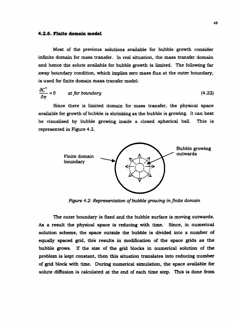
4.2.6. Finite domain model
Most of the previous solutions available for bubble growth consider
infinite domain for mass transfer. In real situation, the mass transfer domain
and hence the solute available for bubble growth is limited. The following far
away boundary condition, which implies zero mass flux at the outer boundary,
is used for finite domain mass transfer model:
ac' -=o at far boundary as
Since there is limited domain for mass transfer, the physical space
available for growth of bubble is shrinking as the bubble is growing. It can best
be visualised by bubble growing inside a closed spherical ball. This is
represented in Figure 4.2.
Bubble growing
Finite domain outwards
boundary
Figure 4.2: Representation of bubble infinite domain
The outer boundary is k e d and the bubble surface is moving outwards.
As a result the physical space is reducing wi th time. Since, in numerical
solution scheme, the space outside the bubble is divided into a number of
equally spaced grid, this resuits in modification of the space grids as the bubble grows. If the size of the grid blocks in numerical solution of the
problem is kept constant, then this situation translates into reducing number
of grid block with time. During numerical simulation, the space avaiIable for
solute diffusion is calculated at the end of each time step. This is done fkom

the knowledge of solution for bubble radius. The resultant space available is
used to calculate the number of grid block, based on the spacing assumed
during initialisation of the solution. These number of grid blocks are then used
while considering solute transfer in the next time step.
A solute balance was done at the end of each time step to calculate the
error in solute balance. Since this technique involves deleting grid blocks, we
end up with some enor in solute balance. It was expected that the maximum
error in solute balance, when the bubble grows 3000 times, shall be 2-3%. In the run the error observed was as predicted. This value is within the
acceptable error Limit.
4.2.7. Modelling solution-gaa M . procer
While simulating the solution-gas drive process (constant volumetric
rate depletion), a certain number of bubbles are considered to be growing in a
specified domain. The growth of the bubble is coupled with the liquid
withdrawn to determine final pressure in the system.
Consider constant volumetric rate production from a porous media
saturated with live oil. During single phase, the average pressure is dropping
at a constant rate determined by singie-phase compressibility. At some point
below the bubblepoint pressure, bubbles nudeate and start growing. Before
critical gas saturation, the system pressure is not only a function of rate of
production but also rate of bubble growth and bubble pressure. In a constant-
volume system, rate of volume expansion of bubbles partly compensates for the
produced liquid and the bubble pressure acts similar to internal pressure
boundary condition, pushing against the liquid.
The folIowing additional equations were used in conjunction with
Equations 4.1 1 - 4.20 and 4.22 to find the solution for the constant volumetric
rate depletion process.

Where, is compressibility of the oil phase, V' volume of oil, Vp pore
volume and B, number of bubbles. Equation 4.23 is the system
compressibility expression. Equation 4.24 states that volume of oil at any t h e
is equal to pore volume minus the volume of gas.
The assumption in equation 4.11 was that the liquid is incompressible,
whereas, in equation 4.23 we consider it slightly compressible. It would be
seen later in the results section that hydrodynamic forces play an ins imcan t
role in bubble growth and hence can be neglected; the hydrodynamic growth
equation can be omitted. Hence the incompressible assumption involved in
derivation of equation 4.1 1 will not change the growth results.
Equation 4.23 is used to calculate the average pressure of the system
after each time step, for constant volumetric rate depletion process. The
calculated average pressure is designated as 9,. This is a good assumption
since in the spherical coordinates, the bulk of the fluid is near the far
boundary.
4.2.8. Physical parameters used in simulation
In this study, oil viscosity values ranging fkom 30 cp to 40,000 cp were
considered. Diffusivity values were taken from AOSTRA handbook and are
given when the results are presented. The di&lsivity for oil of other viscosities
was calculated using the following correlation (AOSTRA (1989))
where X is an empirical constant, V is the molar volume and M is the
molecular weight. Once diffusivity value for oil of a certain viscosity is known,
X is calculated and then equation 4.25 can be used to calculate diffusioiw
values for any other oil viscosity. The initial bubble radius in all cases was I

micron (except while simulating the experiment where it was taken as 0.5
micron). Sensitivity studies were performed on initial bubble radius. Table 4.2
lists the properties that were used in the simulation.
Table 4.2: Parraareterr used in rinrulation of bubble arowth
AU the above equations, for various cases, were solved numerically.
Since the growth equations are non-linear, they were first linearised using
Newton's method poffman (1992)l. Once linearised, the growth equations with
boundary conditions were put into finite difference form. A set of linear
algebraic equations were formed, which were then put in the form of a matrix
and solved using LU decomposition.
The details of calculations, formulation and treatment of the equations
and matrix is given in Appendix - I.
Parameter
Initial Radius
Specific gravity of Oil
Surface tension
Initial solution GOR
H e w s constant
Temperature
Initial no.of space grids
4.3.1. -dual decline in pteuora
Value
1 micron
0.995
0.02 N/m
6.5 v/v
549.5 KPa.mJ/Kg
298 OK
100
4.3.1.1- Infinite domain results
In the simulation run, we started with oil 6 psi (41.36 Kpa) below the
bubblepoint pressure of 600 psi (4136 Kpa) and a gas bubble in e@brium
with the oil. Accounting for capillarg pressure, gas pressure is 600 psi (4136

Kpa) , and the liquid at the bubble interface is at eqyikibrium wi th the gas.
Hence, no concentration gradient exists in the liquid and the bubble and liquid
are in mechanical and chemical equilibrium. Here we have neglected change in
partial molar volume, hence chemical potential of the gas in solution with
pressure. The surface tension of the oil was takm as 0.02 N/m. In the
simulation runs, the gradual decline case was modelled by decreasing the
pressure boundary condition at the far bound- with time (Equation 4.2 1).
The preliminary results indicated that except for unrealistically small
bubble diameters, the surface tension forces did not have any significant effect
on bubble growth in the heavy and light oil. Szekely and Martins (1971)
reported similar results. Surface tension force, although accounted for in the
initial equilibrium of the bubble and liquid, is hence neglected in the growth
process.
Figure 4.3 compares the general growth case, including both
hydrodynamic and diffusive forces, to diffusion-limited asymptote, for pressure
dedine at rate of 100 psi@ (689.3 Kpalhr). The two results match each other
exactly. This is in line w i t h some previous conclusions [Szekely and Martins
(1971). Szekely and Fang (1973)j that, except for very early times, the
hydrodynamic forces do not play a significant role in bubble growth, and the
model considering diffusive forces done can be sufficient to predict the gas
phase growth. Throughout this study and for generality of concIusions,
calculations are performed using the general growth model.
The results shown in Figure 4.4 are for thc growth of bubble for three
oils of viscosities 30 cp, 2000 cp and 40,000 cp, when the pressure drop rate is
100 psi/hr (689.3 Kpa/hr). It may be noted that for light oil (30 cp) we observe
the bubble grows by about an order of magnitude in the first minute whereas
for a heavy oil of 2000 cp and 40,000 cp we may not see a considerable change
in the size of the bubble in the first 2 and 100 minutes, respectively- In
simulation runs of figure 4.4 a s i o n coefficient was changed alongwith
viscosity based on equation 4.25. It is still desired to investigate if the different
results in Figure 4.4 for different oils is due to oil viscosity or diffusion


coefficient. The results for the effect of diffusion coefficient shall be presented
later.
It can also be seen in the Figure 4.4 that once the bubble growth starts,
it almost follows a straight line on a log-log plot for all the cases. We can
deduce that the bubble growth may be modelled by the relationship R(t) = atb
for R > 4 . The constant a determines the initial delay observed in Figure 4.4.
This delay plays an important role in the pressure behaviour of the two-phase
system, as we shall see later. The above power-law model was previously
suggested for the cases when the process was limited by one of the forces only
[Kashchiev and Firoozabadi (1993)j. Here, its applicability is demonstrated for
the general case where both hydrodynamic and diffusion terms are considered
and pressure is gradually decreasing in an infinite domain, although it has
already been shown that the process is governed by diffusive forces. The
results depicted in Figure 4.4 suggest that the constant a is a function of oil
type, for the same rate of pressure drop.
The simulations were done for the case when the pressure depletion rate
was taken to be 100 psi/hr (689.3 KPa/hr). This, when compared to the field
pressure depletion rate, is quite high. Cases with lower rate of pressure drop
are discussed later (see Figures 4.6 and 4.1 1).
In Figure 4.5, bubble growth is compared for the two cases of step
change and gradual decline in pressure. The step decline in pressure is
simulated by dropping the pressure at the far away boundary suddenly by 540
psi (3722 ma) , from 600 psi (4136 Wa) initial pressure. The initial bubble
growth in case of step decline in pressure is much greater than in the case
when the pressure is lowered gradually. This is because, in step decrease in
pressure, the concentration and the pressure driving forces are much greater
than that in case of gradual dedine of pressure, where the concentration and
pressure driving forces increase slowly wi th time.
Resuits of Figure 4.5 indicate that for the same oil, constant b is rather
insensitive to method of pressure drop, for exampLe the exponent b is estimated
to be 1.04 and 1.32 for the step dedine and the gradual decline cases,

100 1000 loo00 100000 Time, sec
Figure 4.6: Effect of depletion rate on bubble growth

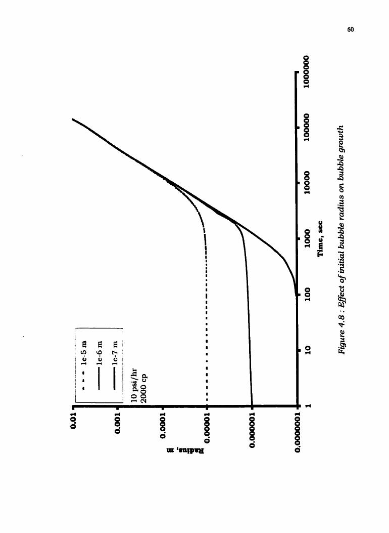

respectively. The value of a which is a measure of the "delay", varies with
change in depletion rate; increasing with increase in depletion rate, i.e.,
reduced delay.
The effect of pressure decline rate on the growth is shown in Figure 4.6.
It is observed that for aU the cases the slope is same. Hence it can be
concluded that the constant b is independent of rate of pressure decline for the
same oil. Further, it is apparent fkom the graph that constant a is a function of
pressure decline rate. The constant a follows a logarithmic trend with pressure
depletion rate as shown in Figure 4.7. A similar behaviour for a and b had
been suggested in other studies Firoozabadi and Kashchiev (1996)j on bubble
growth.
The effect of initial bubble radius on bubble growth is shown in Figure
4.8. It is evident that at late time a l l the radii converge to a single value
asymptotically. This is in conformance with the experimental study of Yousfi et
aL(1997), where the bubble radius, with respect to time, was reported to be
independent of initial bubble radius. Hence, the parameter a and b are
insensitive to initial bubble size for the range of time studied.
The significance of results of Figures 4.4 - 4.8 is to show that if bubble
growth experiments are used to develop empirical correlation of the type of atb,
experiments should be properly scaled because these constants are functions
of oil properties, rate of pressure drop etc. Laboratory experiments with rates
of pressure drop much higher than those observed in the field [Sheng et aL
(1999)j and under different conditions can not be used for field predictions.
Further, this single atb model for all times is valid only for infinite domain - not finite domain as we shall see below,
4.3.1.2. Effect of no-flow boundary
In the simulation run, this was done by assigning a dosed domain for
mass transfer and a zero concentration gradient at the far boundary. This was
shown in the mathematical formulation earlier (Equation 4.22) and is given in


detail in Appendix -I. What this translates to in the transformed co-ordinate,
which moves with the bubble-intedace, is that, although the bubble boundary
remains stationary the outer boundary moves inwards with time. In Figure 4.9
comparison is done for cases of bubble growth in i nh i t e and finite domain. It
is clearly evident fkom the figure that, at late times, the model for bubble
growth in infinite domain is different from that of no-flow boundary. The
discrepancy starts when the concentration disturbance reaches the outer
boundary in no-flow boundary case. Looking at the trend, it might be infixred
that the no-flow boundary growth does not foUow the a t b model. More results
on bubble growth behaviour in a dosed system are presented in the following.
4.3.2. Gam phase build-up druing solution-gas drive
In this section, we report the results obtained fkom the application of the
growth model thus developed, to the above physical problem. During early
stages of gas evolution, and much before critical gas saturation is reached,
bubbles are neither in contact nor flowing - conditions pertinent to our
mathematical model. W e have used the above model to study the pressure
behaviour observed in constant rate of depletion experiments pooladi-Darvish
and Firoozabadi (1999)1, in particular, the seqyence of increasing
supersaturation below bubblepoint pressure, bounce in system pressure and
the final reduced supersaturation. Similar behaviour has been reported in
some of the other studies Firoozabadi and Kashchiev (1996), Guo-Quig and
Firoozabadi (1999)l. One assumption in extending our growth model to the
above problem is that the effect of porous media on growth is neglected and the
bubbles are assumed spherical. Also we have assumed that a l l bubbles
nucleate at the same time below bubble point pressure, and no further bubbles
nucleate afterwards. More on this assumption is given in Section 4.4. The
simulation starts at the pressure where the bubbles are assumed to be
nucleated. The P-V behaviour before nucleation is calculated separately using
the single phase system compnssibility.

The results discussed below, show that the system supersaturation
increases even after bubbles have nucleated. This provides more d r i . g force
for fur ther nucleation, VioIating the above assumption. Here, we ignore the
short time when supersaturation is increasing and assume that instantaneous
nucleation is a valid assumption [Kashchiev and Firoozabadi (1993)l.
4.3.2.1. Results
In Figure 4.10, we show predictions of our numerical model for the
experimental conditions of Pooladi-Darvish and Firoozabadi (1999). The
bubblepoint of the oil in the above study was determined as 363 psig (2502
KPa) (by extrapolating equilibrium line backwards). In the model developed it
has been assumed that the bubbles generated at 351 psig (2419 KPaJ (a
supersaturation of 12 psi (82.7 Wa), which corresponds to an initial bubble
size of 0.5 micron). 250 bubbles were assumed, corresponding to roughly 1
bubble per cmJ of pore volume. This approximate value of number of bubbles
is in line, with that predicted by Kennedy and Olson (1952). The growth of the
bubble and the system pressure were studied with respect to volume of fluid
withdrawn. Table 4.3 lists the parameter and properties that were used in
simulation.
Table 4.3: Parameter wed in rimulatiap errperimental data of Pooladi-
Darvlrh and Fimozabadi (19991
Parameter
Viscosity
Depletion rate
Number of bubbles
Initial bubble size
Pore volume
Dmsiv i ty coefficient
Initial GOR
Vdue
34,000 cp
lcc/ day
250
0.5 micron
245 cc
5 x 10-Io m2/s
6.5 v/v


The data are those given by Pooladi-Darvish and Firoozabadi (1999)
except the initial bubble size and diffusivity coefficient, which were not
reported in the original reference. All other parameters were the same as those
listed in Table 4.2.
Figure 4.10 shows that although the bubbles had nucleated at 35 1 psig
(2419 KPa), the pressure continued to fall at the same rate. This means that
the system compressibility, defined earlier as:
is equal to single-phase compressibility even after bubble generation. In
some of the previous works [Pooladi-Darvish and Firoozabadi (1999),
Firoozabadi and Kashchiev (1996)l it was implied that the bubbles do not
nucleate until we reach the lowest point in the depletion P-V curve. The
authors argued that earlier nucleation of bubbles would have been reflected by
the change in system compressibility and hence change in the slope of P-V
graph. Here the results from our model show that even after generating
bubbles, the pressure in the system can drop and can follow the single-phase
compressibility curve. This might be explained by the delay present in the
early times of bubble growth, evidenced in Figures 4.4 and 4.6. During the
early time, rate of bubble growth is negligible so the rate of pressure drop is the
same as that for the case of single-phase fluid. This early time behaviour, in
part, can be attributed to smaller surface area available for mass transfer at
early times when the bubble is smaller. This is abetted by the fact that the
diffusivity coefficient is low for heavy oils. Later, when the P-V curve
approaches the lower most part, the pressure drop line becomes more gradual
as the growth of gas phase increases.
The time delay in bubble growth, which is the time after which the at*
model is valid, is not apparent in the gas phase growth model put forward by
Firoozabadi and Kashchiew (1996). They appIy this model as soon as the
bubbles nucleate. Thus the pressure in their system rises as soon as bubbIes
nudeate.

Our model does not dip as much as the experimental results and does
not match the data when the system pressure starts recovering. This might be
due to the assumptions in the model: neglecting effect of porous media on
growth and instantaneous nucleation. Sensitivity studies were performed to
accurately fit the experimental data with the cumnt model. The variable
parameters were number of bubbles, a s i o n coefficient and nucleation point.
It was observed that lowering the nucleation point or diffusion coefficient or
number of bubbles would dip the curve fiuther down, but then the rebounding
would take a long time. No significant improvement in the quality of the model
was observed.
During the later stage of the process the model matches well with the
experimental result. This is because an eqyilibrium state wi th respect to mass
transfer has been attained and there is negligible mass transfer driving force in
liquid phase. The negligible mass transfe~ driving force was evident in the
concentration results, where the solute concentration at gas-oil interface was
equal to that at the far boundary. It is the continual pressure drop at the far
boundary that makes more gas available for bubble growth. huther, the two-
phase compressibiIity, assuming e m b r i u m condition, as given by the
following equation [Ramey ( 1964)]
where, is the total, or two phase (gas and oil) formation volume factor:
fl, = A + (Rmr - )P, (4.28)
is found to be 8.31 x 10⁻⁴ psi-' (1.2 x 10⁴ KPa-I). This equals the
experimentally observed two-phase compressibility of the system, which is 7.54
x 104 psi-1 (1.1 x 10⁻⁴ Pa-1). This eqyality of the two values may indicate state
of equilibrium.
Here, our intention was not to match the experimental data, which is
governed by nucleation and growth physics in porous media. The arbitrary
numbers chosen for matching purposes, i.e. nucleation supersaturation of 12
psi (82.7 m a ) and bubble density of 1 per d, might be modified once a better


understanding of nucleation physics and the effect of porous media on
nucleation and growth is known. The intention was to show that system
compressibility might remain unchanged for some time wen whiIe bubbles are
growing.
4.3.2 -2. Sensitivity studies
4.3.2.2.1 Effect of depletion rate
The effect of rate of depletion is shown in Figures 4.11-4.12. It is evident
that as the depletion rate increases, the pressure dips further down. This, in
earlier studies [Kennedy and Olson (1952)], was assumed to be an indication of
the increase in critical supersaturation before bubbles nucleated. Here we
again show that, even though the bubbles nudeate much earlier at 351 psig
(2419 ma), the pressure keeps on dropping. The results clearly indicate that
with increase in depletion rate, a lower pressure is obtained before pressure
starts retrieving. A pressure difference that can be termed as "Apparent
Critical Supersaturation".
Many of the previous studies had observed higher apparent critical
supersaturation at higher rates of pressure drop. Our results suggest that,
could be partly explained by the growth physics in contrast wi th nucleation
physics.
Finite us. Infinite:
Figun 4.12 shows the bubble radius as a function of produced volume
(which is a multiple of time). It is obsemed in this graph as well as in Figures
4.14 and 4.16 that bubble growth behaviour is different than that observed in
an infinite medium. Hence, the results of bubble growth studies in W t e
domain [Scriven (1959), Szekely and Martins (1971), Szekely and Fang (1973),
Rosner and Epstein (1972), Patel (1980)], which w u e used in growth studies in
porous media mchiev and Firooabadi (1993). Firoozabadi and Kashchiev


(1996)l might be valid only before the effect of concentration at the far
boundary in felt.
Once again considering the model growth of atb, Figure 4.12, 4.14 and
4.16 suggests that after an early time of large b, where the concentration at the
far boundary has not been affected, the exponent decreases and all the graphs
converge to a single lower value of b, which is approximately equal to 0.5.
4.3.2.2.2. Effect of viscosity
The effect of oil viscosity is shown in Figures 4.13-4.14. For a large
range of viscosity of oil, with similar diffusion coefficient, it is observed that all
the results are same i.e there is no effect of viscosity. For further veritication of
the viscosity results shown in Figure 4.13, a model was run with only
a s i o n a l term and the results were compared. As can be seen in Figure 4.13,
the diffusion model lies on top of all other cases. This dearly demonstrates
that diffusional forces dominate the process of bubble growth in the real field
time scales.
4.3.2.2.3. Effect of diffusion coefficient
The effect of diffusion coefficient on depletion process is shown in
Figures 4.15 and 4.16. The higher diffusion coefficient leads to faster retrieval
of pressure and lesser "Apparent Critical Supersaturation". .s can be
explained by the fact that initially the bubble grows faster in case of oil with
higher diffusion coefficient (shown in Figure 4.16). At later time the bubble
radius for a l l the cases starts reaching an asymptotic value but the amount of
gas in bubble is different. This leads to diffixent bubble pressure, which is
being exerted on the liquid. Although bubble radii approaches the same value
after some time, pressure is lower in lower diffusivity oils. So for the same rate
of depletion in light and heavy oil, the higher =Apparent Critical

Supersaturation" in heavy oil can be attributed, in part, to the lower diffusivity
coefficient of heavy oil.
In a recent study [Tremblay et al. (1998)] no bubble was observed to form
for about 3 hours after the pressure in a 30,000 cp live oil system was
decreased from 780 psi (5170 KPa) to 500 psi (3446 m a ) in one step ( P, = 750
psi (5170 KPa)). One of the possible explanations for this anomaly could be
that the supersaturation effects were large and no bubble could nudeate. A
second explanation can be provided using the model of this study. The model
was used for the above oil and it was found that the bubble, if nucleated, would
grow to a size of about only 10 pm, starting from initial bubble size calculated
for supersaturation of 250 psi (1723 KPa) [Brennen (1995)], in about 3 hours.
Our model applies to growth in bulk, and it is expected that the porous media
would further restrict the growth of bubbles. Our results suggest that the time
kames might have been insufficient for noticeable growth of the bubbles and
gas bubbles were possibly very small.
One assumption in our study is that nucleation is instantaneous. A
number of researchers [Firoozabadi and Kashchiev (1996), Yousfi et al. (19971,
Crum (1982), Wilt (19891, Coles (1974), Stewart et at. (1954)j have studied this
phenomenon. Yousfi et aL(1997) studied the nucleation in micro-model and
concluded that the nudeation is not progressive after a brief initial time since
the number of bubbles reach a plateau after some initial time and the rate of
bubble generation becomes zero. huther, in line wi th their observance of
increasing number of bubbles at initial time, they conduded that the theory of
instantaneous nucleation does not hold at early times. The same is also
evident from the study of Stewart et aL (1954). Conversely, with the theory of
pre-existing bubbles [Wilt (1989). CoIes (197411, due to presence of stabilized
bubbles, the process of nucleation can be assumed to be instantaneous. Wilt
(1989) in his study showed that the progressive process could result in very

small size of the bubbles and hence nucleation can be considered
instantaneous. Yousfi et al. (1997) from their study concluded that if we
disregard the initial time when the bubbles are being generated, which is
negligible compared to field times, the assumption of instantaneous nucleation
is valid. In our modelling we have adopted the instantaneous nucleation
assumption.
4.5. One pouible acenario of bubble genedon
When the pressure is lowered below the bubblepoint pressure and there
is no formation of free gas phase, the oil becomes supersaturated. When
supersaturation becomes large enough bubbles nucleate and those larger than
a critical radius start to grow. The growth of the bubble can be dominated by
hydrodynamic forces, mass transfer forces or both, at least at early time. Since
the di&tsion coefficient is typically low in heavy oil, the rate of increase of
supersaturation due to pressure decrease could initially be more than the
decrease in supersaturation due to diffusion of gas into the bubble. This is due
to the fact that the concentration disturbance has not reached the fa
boundary. As a result the supersaturation at a point far away from the bubble
goes on increasing. This is especially true, before system pressure starts the
upward trend. Due to further increase in supersaturation, the threshold value
requind for the nucleation to occur may be met at the far away point. Thus a
new bubble nucleates which starts lowering down the local supersaturation.
The time required for this process may be small compared to the field time and
hence instantaneous nucleation may be a good assumption [Yousfi et al.
(1997)l for aU practical purposes, whereas in reality and microscopic sense the
nucleation process may be progressive. Since the diffusion coefficient in light
oil is greater than in heavy oil, it is expected that decrease of supersaturation
s h d be more in light oiI than in heavy oil. This leads to conclude that the
number of nucleated bubbles s h d be more in heavy oil than in light oil. This
is in h e with the experimental results of Pooladi-Darvish and Firoozabadi

(1999), where a larger number of bubbles were observed in their heavy oil
experiments than that in light oil experiments.
The increase in the number of bubbles during solution gas drive has
been shown to increase the recovery factor [Stewart et al. (1954)l. This could
also be one of the factors responsible for the favourable behaviour of heavy oil
reservoirs.
Whether supersaturation and the kinetics of nudeation and growth are
important under field condition is still unresolved. Batycky et aL (1997) in
their work gave clear evidence of sigdicant supersaturation in the reservoir.
Solution gas drive in porous media involves nucleation, bubble growth
and flow. Further studies would clarify the interaction of these phenomena
and the effea of presence of porous medium on the process.
A numerical model was developed for growth of a single bubble in heavy
oil and light oil for gradual decline in pressure. The results for the cases
studied indicated that:
1. Viscous forces, and in general hydrodynamic forces, have little or no
effect on bubble growth in heavy oils at late times. Modelling bubble growth in
heavy oil using ditfusion equation only, can be a valid approximation after an
early time of the order of seconds to minutes. Rate of growth of a bubble in
heavy oil is much less than that in light oil.
2. For bubble growth in infinite domain, the application of the growth
model of R(t) = atb for could be extended to the cases where both
diffusional and hydrodynamic forces are acting. However, if experiments are
conducted to determine constants a and b, these need to be properly designed
to represent the actual case of interest. It was shown that the constants
depend on numerous parameters such as diffusion coefficient and rate of
pressure drop. More over, modelling of bubble growth in dosed domain
showed that this simple power law model might not adequately describe bubble
growth behaviour.
3. By applying growth model to one set of solution gas drive experiment
it was shown that even though the bubbles nucleated earlier, the system
pressure decreased before retrieving after reaching the "apparent critical
supersaturation" pressure. Hence, the assumption that bubbles nudeate at
the apparent critical supersaturation might not be correct. The apparent
critical supersaturation depends on bubble nucleation as well as bubble
growth kinetics.
4. I t was found that higher depletion rate and lower diffusion coefficient
result in a larger difference between nucleation pressure and the apparent
critical supersaturation pressure. This could explain higher supersaturation
obtained in heavy oil experiments (lower difiusivity) and those with higher rate
of pressure drop.

Chapter 5
GAS MOBILITY MEASUREMENT
The process of solution gas drive involves nucleation of the gas bubbles
followed by bubble growth and coalescence and finally flow of gas.
As mentioned previously, the heavy oil resexvoirs in Alberta and Western
Saskatchewan under solution gas drive show anomalous behaviour when
compared to conventional light oil reservoirs. At least one of the theories
[Pooladi-Ddsh and Firoozabadi (1999), Guo-Quig and Firoozabadi (1999)l
attributes this favourable behaviour to low gas phase mobility in heavy oil. The
low gas mobility implies lower gas velocity that results in gas retention and
pressure maintenance in the reservoir. Fiially, all these factors lead to higher
oil recovery.
In this part of the thesis, experiments were done on unconsolidated sand-
pack at various depletion rates and the effect of rate of depletion on critical gas
saturation and supersaturation was studied. Further, the experimental results
were used to determine mobility of gas phase at various depletion rates.
Production and pressure data obtained &om depletion was matched on a
commercial reservoir simulator by adjusting critical gas saturation and gas
relative permeability values.
The chapter starts by describing the experimental setup and procedure.
Next, the experimental results are presented. Simulation of the experiment
and analysis of the results follow the results. Towards the end of the chapter, a
brief discussion is presented which is followed by condusion.

5.2. Experimental setup
The experimental setup consists of an Isco syringe pump, a multiple
pressure port core holder with viton sleeve that encases the sand pack, gas-
liquid separator (Visual cell), overburden and axial pressure system, piston
cylinder for transfer of Live oil, a recombiner for preparation of live oil, constant
temperature air baths and a vacuum pump. The instruments used for data
acquisition are pressure transducers and thermocouples. A LabTech (1994)
notebook is used to record data from various instruments during the
experimental run. The schematic of the experimental setup is shown in Figure
5.1,
The core holder is made of titanium and encases the Viton sleeve that
contains 60 cm long sand-pack. There are 3 pressure taps in the core-holder,
connected to pressure transducers to measure the differential pressure in the
various sections of the sand-pack. The reading accuracy of the differential
pressure transducers is i 0.025 psi (0.17 ma). The picture of the core-holder
is given in Figure 5.2.
To avoid any effect of gravity, that may lead to segregation of gas and oil
in the core during experiments, the core-holder is rotated 180 degrees every 15
minutes.
The outlet end of the core-holder is attached to a visual ceU. The visual
cell, which is 10 cc in volume, has a long window on both sides so that the gas-
oil intedace is clearly visible for production measurement. The small size of
the separator is selected to minimize the dead volume. This ensures that
almost all of the gas collected in the visual cell is corning from the sand-pack
and negligible amaunt of the gas is being generated in the oil in the visual cell.
The picture of the visual cell is shown in Figure 5.3. The outlet, kom the
bottom of the visual cell, is connected to the Isco pump.
Other equipment required are a recombiner for the preparation of the
live oil and a transfm cylinder for the transfer of h e oil &om recombiner to the
rsco pump*

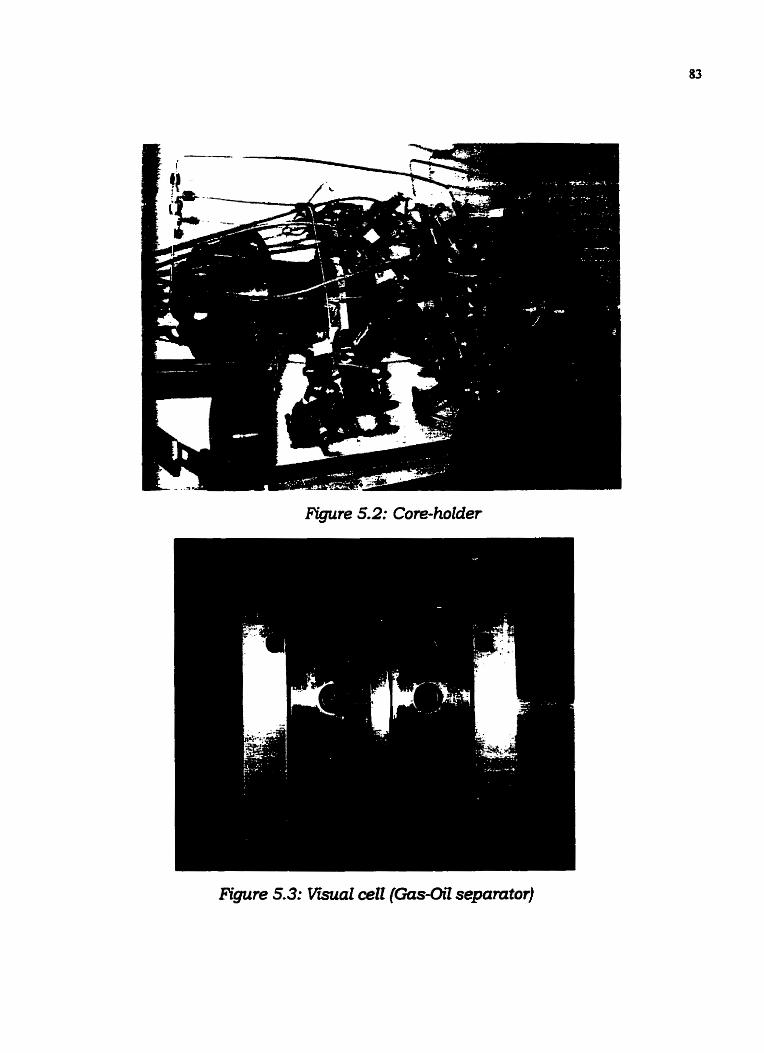
Figure 5.2: Core-holder
Figure 5.3: V i a l cell (Gas-017 sepamtor)

The overburden and axial pressure system comprises of a hand-pump, a
buffer piston vessel and a backpressure regulator. Water is used as the
overburdm/axial pressure medium. The hand-pump is used to build up the
pressure during start-up. A buffa piston vessel with nitrogen on one side,
connected through a backpressure regulator to the nitrogen supply cylinder, is
used to dampen pressure fluctuations that may be introduced due to
temperature fluctuations.
The core-holder and visual cell is placed in a constant temperature bath.
A temperature controller acting on a hot air blower is used to control the
temperature in the bath. The temperature in the bath is conttolled within an
accuracy of k 0.1 Deg C.
5.3. Florid data
A poly-alphaolefinic type (PAO-100) of synthetic hydrocarbon oil (From
Nye Inc.), with spedfic gravity of 0.85 and dead oil viscosity of 2552 cp at 25
Deg C, is used. The dead oil viscosity is measured with a Haake-PK100 cone
and plate viscometer. The GOR of the live oil was measured to be 15.57 vol/vol
at 25 Deg C. Methane is used as the gas phase in all the experiments.
Properties of the live oil are shown in Table-5.1
For measurement of live oil viscosity, a flow loop is made at the inlet of
the sand-pack. The pressure drop across the Ioop is used to determine the
viscosity. Thus, it is possible to measure viscosity of the fluid inline.
Table - 5.1: Pmpertv of fluid
- P ~ W Oil
Dead Oil Viscosity @ 250C
Live Oil Viscosity @ 25oC
Specific Gravity
GOR @ 25oC
Bubble Point
Value
PAO- 100
2552 cp
1100 cp
0.85
15.57 v/v
575 psia (3963 KPa)

5.4. Experimental procedure
5.4.1. Hydro-testing of the vessels
AU the vessels to be used in the experiment were hydro-tested to a
pressure equal to 1.5 times the maximum operating pressure in the system.
This was done to ascertain the mechanical health of the vessel and avoid any
leakage or failure of the vessels during experimental run.
5.4.2. Calibration of transducers
The absolute pressure transducers and digital pressure gauges were
calibrated using dead weight tester. The Sensotech differential pressure
transducer was calibrated using the calibration method specified in instruction
manual. The range of measurement of differential pressure transducer is 10-
15 psid and reading accuracy is k 0.025 psi (0.17 Wa). The differential
pressure transducer is designed to operate wi th liquid on both the sides, so it
was made sure that both the chambers were free of air (completely liquid filled).
This was done by filling it with Bayol (A light oil) prior to connecting it to the
system.
5.4.3. Over pressure controls
The running of experiments required safety to be one of the major
concerns. The system was eqpipped with proportional pressure relief valves,
set at relieving pressure depending on the maximum operating pressure and
design pressure of the equipment and piping/fitting. The Isco pump control
software also has an inherent feature through which the safety pressure setting
can be set. The outlet piping of the pump is equipped wi th pressure relief
device to ensure additional safety. W the pressure safety valves were set at the
proper relieving pressure by flowing light oil (BayoI) through them using the

86
Quizix pump, at constant flow rate. The discharge pressure was adjusted by
tightening or loosening the spring of the pressure relief valve. This pressure
then becomes the relieving pressure.
5.4.4. Data acquisition and control
A Labtech notebook (1994) was used for data acquisition from the
various pressure transducers and thermocouples. A program was written to
acquire the required data and display it on the screen in digital as well as
graphical form. Further, this data was also recorded in a file that could be read
on a worksheet.
5.4.5. Temperature control
The oil used in the experiment, being highly incompressible, exhibits a
si@cant change in pressure due to small change in temperature. So it was
imperative to maintain a constant temperature during the experiments.
The big cabinet housing the core-holder is equipped wi th a temperature
controller acting on a heater. The temperature in the smaller Blue-M oven was
controIled by a temperature controller acting on In-car heater that was placed
in the oven. Both the ovens were equipped with circulating fans to have a
uniform temperature across the oven. The temperature of the fluid in Isco
pump barrel was controlled by a similar controller acting on a heating tape that
was wound around the pump barrel. Further, the pump barrel was insulated
to avoid any heat loss. The flow Lines were insulated to prevent any heat loss.
The temperature controllers were equipped with over temperature control that
trips the system if the temperature exceeds the safety set point.
5-4.6. Calibration of visual cell
The gas and oil produced from the core is separated in the visual cell.
The amount of gas or oil produced is measured by measuring the gas-oil

87
interface. So it is necessary that the visual cells be calibrated. The height of
the interface was measured with a cathetometer, which was mounted outside
the oven. A high intensity light was thrown &om the rear window of the visual
cell which facilitated the measurement of gas-oil interface in visual cell. The
visual cell was calibrated with the Quizix pump. The calibration was done by
recording the reading on the Cathetometer scale against the volume of the fluid
injected in the visual cell, which was measured by Quizix pump. A plot was
generated with the above data of volume vs. height on the cathetometer.
5 -4.7. Sand preparation and packirig
Rior to packing in the core, the desired sand was sieved with a sieve
shaker through 200 mesh screen. The undersize was then sieved through 325
mesh screen, The oversize from this screen was taken as the product sand to
be used in packing of the core. The grain size distribution of the sand thus
obtained was between 50 and 75 pm. The desired sand was then extracted for
five days using a 1:l mixture of Methylene Chloride and Methanol. This was
done to remove any impurities and have a total water wet sand. This was
camed out in a round bottom flask, where the liquid mixture was at the bottom
and the sand was held in the neck of the flask in cylindrical cellulose
containers. The flask was then heated by providing controlled heat through a
rheostat. The vapours &om the bottom of the flask extracted the sand and
then were condensed at the top in a total condenser. The condensed liquid
would then flow back into the bottom of the flask. The setup is shown in
Figure 5.4. Once the extraction was over the sand was taken out and dried to
remove traces of solvents.
The sand is then packed in Viton sleeve, which is inserted into the core-
holder prior to packing. The main body of the coreholder consists of five basic
parts: the pressure cell body, the stationary end, the piston end and two
collars. The sleeve materid used for the coreholder was viton.

Figure 5.4: Sand extmction setup
Figure 5.5: Vion sleeve with multiple pressure taps

Table - 5.2: Propem of md-Pack
To pack the coreholder with sand, first the collar was installed on one
end of the sleeve. Subsequently, the pressure cell was mounted on to the
rotating stand. The sleeve and stationary end was then inserted into the
pressure cell, aIigning pressure port on sleeve with those on core-holder. A
picture of sleeve is shown in Figure 5.5. The stationary end was locked in
place. The dry sand was then vibrated into place leaving room at the top for
the piston end. A thin layer of coarser sand grains was used at either end
while packing the sand. This is done so that a screen larger than the grain size
of the sand-pack can be used and yet migration of sand into the outlet stream
can be avoided. The larger screen size prwents build-up of gas at the outlet
due to trapping of gas bubbles [Pooladi-Darvish and Firoozabadi (1999)], which
could happen if screen size s d e r than the sand grain size is used. The
property of the sand-pack is given in Table-5.2.
The sand used in filling was weighed to measure the length of the sand
pack. Any sand particles that may have accumuIated on the upper portion of
the sleeve material were removed to ensure proper seal. The second collar was
inserted into the end of the sleeve. CarefUy the piston end was inserted into
the collar and sleeve and locked in place.
R0p-W
Length of the Sand-Pack
Pore Volume
Porosity
Absolute Permeability
Effective Permeability
Connate Water Saturation
Sand Grain Size
Overburden/Axial Pressure
Compressibility
Value
60 cm
487 cc
38.6 %
1.24 Darcy
1.18 Darcy
2.1 %
50 - 75 Micron
1 120 psig (7720 m a )
2.2 x 10⁻⁵ psi-1
(3.2 x 10⁻⁶ KPa-1)

5.4.8. Rotating Core-holder
I t was decided to rotate the core-holder to minimise the gravity effects.
For this purpose, the core-holder was mounted on swivel joints on both ends.
A DC motor with gear box having a gear ratio of 15 125: 1 was attached to rotate
the core-holder approximately 180 degrees once every 15 minutes.
5.4.9. De-aerating water
It is important to ensure that the water, to be used in leak test and in
flooding the core, contains no air (fkee of compressible fluid). This was done to
avoid any confusion arising during leak test, because of pressure drop due to
dissolution of air in water- The de-aeration was done with bench vacuum in
the lab and agitating liquid in the flask by magnetic stlrer.
5.4.10. Applying Overburden and Axial Pressure
Once the sand-pack was prepared, overburden and axial pressure was
applied simultaneously with a hand-pump, by teting off the line from the pump
outlet to overburden and axial pressure connection on the core-holder. The
overburden and axial pressure was built-up to 1 120 psig (7720 m a ) in steps of
50 psig (345 KPa). Water was used as the fluid for applying overburden and
axial pressure. Once the pressun was built, a piston vessel containing water
on one side and nitrogen on other side was used as a buffer vessel. The
nitrogen in the bufEer vessel was attached to the nitrogen tank through a back
pressure reguIator. Buffer vessel was used to dampen pressure fluctuations, if
any, that occur from temperature fluctuations. The pressure set point, of the
back pressun regulator, was set epuaI to the overburden/axiaI pressure. The
back pressure regulator helped in maintaining a constant overburdm/axial
pressure on the sand-pack,

5.4.11. Leak test
Once all the piping and core-holder was set in-place, the next step was
to leak test the system. For the piping, this was done by isolating a section of
piping, pressuring it up with water and observing the pressure in the section,
under isothermal condition. A leak fkee system would indicate no pressure
drop with time. The leak test in the sand-pack was done with nitrogen gas.
This was done to avoid wetting of the sand-pack prior to measurement of pore
volume.
5.4.12. Vacuuming of pumps/system/sand pack
Once the whole system including the core-holder was leak tested, the
water fkom piping was drained. ,9 vacuum pump was then used to draw
vacuum of 10 mTorr. The catch-pot before the vacuum pump inlet was kept in
dry ice to achieve such high vacuum. The vacuum pump was run for 24 hours
to achieve such high vacuum. The vacuum was pulled to remove any air that
might get trapped during flooding of the system, while measuring the dead
volume. The trapping of air has two-fold affect. One, it increases the
compressibility of the fluid and secondly, it gives erroneous estimation of dead
volumes.
5.4.13. Volume measurement by water
Once the system was vacuumed, the water was introduced into the
system by pumping with Isco pump. To measure the volume in each section of
the piping the water was introduced into the system section by section;
isolating a paftidar section fkom rest of the vacuumed system by dosing the
valve. Once a part idat section was filled with water, the pressure was raised
to 100 psig (689 ma). The dii3erence in volumetric reading indicated the
vohme in that section.

5.4.14. Porosity and absolute permeability measurement (saturation of core)
Next, the vacuumed sand pack was flooded with water to measure the
pore volume and hence the porosity of the sand-pack. The porosiw was found
to be 38.6%.
Once the sand-pack was flooded with water, the valves connecting to the
pressure transducers were opened. Water was flowed through the sand-pack
at a known rate and the pressure drop across the core was measured for
determining absolute permeability of the sand-pack. This was done at several
flow rates to have an average value. The Darcy's equation in the following form
was used to determine permeability
Here, q is the flow rate, AP is the pressure drop across the sand-pack, L
is the Iength, A is the cross sectional area and p is the viscosity. A plot was
generated, shown in Figure 5.6, and the slope was found to determine
permeability. The value of the absolute penneability was found to be 1.24
Darcy.
5.4.15. Connate water saturation and effective permeability measurement
(flooding with dead oil)
Once the sand-pack was flooded with water and absolute permeability
was determined, the dead oil was flooded into the sand-pack displacing the
water. The dead oil was injected until no additional water was produced fkom
the outlet end. The oil and water thus produced weze measured to determine
the connate water saturation in the sand-pack. The connate water saturation
was found to be 2.1%.
Once the inlet piping to the core-holder and the sand-pa& was flooded
with dead oil, the dead oil was flowed through the sand-pack at a h o w n hw
rate and the differentid pressure across the core measured to determine the

Figure 5.7: Detemihution of Effective kknrre-

effective permeabilie of the sand-pack. A similar plot as discussed for absolute
permeability was generated. The plot is shown in Figure 5.7. The effective
permeability of the sand-pack was found to be 1.18 darcy.
Once the core was flooded with dead oil, the rest of the system
comprising of visual cell and piping was flooded with dead oil displacing water.
5.4.16. Measurement of dead oil viscosity
The viscosity of the dead oil was measured at various temperatures
using a Haake PK-100 cone and plate viscometer. The picture of the
equipment is shown in Figure 5.8. The viscometer was hrst calibrated with a
fluid of known standard viscosity at a given temperature. The temperature was
maintained by a heatingJcooling bath. Next, the dead oil sample was put
under the disc and the torque measured at a specified RPM. This data was
used to calculate the viscosity. This was done at various temperatures.
Further, a log-log viscosity vs. temperature graph was plotted to predict
viscosity of the dead oil with temperature. The experimental data is given in
Table 5.3 and the result graph is shown in Figure 5.9.
5.4.17. Viscosity loop calibration
It was desired to measure in-line viscosity of live oil during the
experimental run. The viscosity was measured in-line by measuring the
pressure drop in a certain section of a coiled tube and then calculating the
viscosity using the Hagen-PouisUe Equation w a b e , Smith and H d o t
(1990)j for flow through pipes which is expressed as
16 where f is the fkiction factor. For laminar flow f = - where Re is the Re
ReynoIds numba which is expressed as

Figure 5.8: Haake PK-100 viscometer
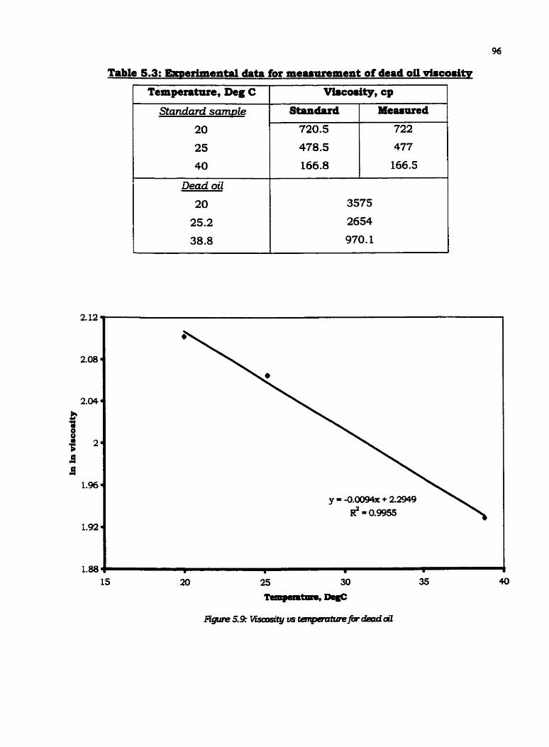
Table 5.3: merimental data for measmment of dead oil viscoritv
Temperatuse, Deg C
Standard sarn~le
20
25
40
Dead oil
20
25.2
38.8 7
Vbcooity, cp
Standard
720.5
478.5
166.8
Measured
722
477
166.5
3575
2654
970.1

substituting this in Equation 5.2 and simpli&ing we get
Here, the initial part on the RHS in the parenthesis is a constant and
depends on the geometry of the flow loop (geometric factor). This constant was
determined by calibrating the flow loop with fluid of known viscosity viz. water
and dead oil.
The dead oil and water of known viscosity were flown through the loop
and the pressure drop across the loop was measured. Knowing the viscosity,
this data was then used to determine the geometric constant of the loop.
5.4.18. Measurement of compressibility of dead oil
The compressibility of the dead oil was determined by compressing it in
the cylinder of the Isco Runp and recording pressure versus the volume data
(P-V data). The data was then plotted on a graph and the slope of the line was
used to calculate the compressibility using the following formula:
The P-V graph for determination of dead oil compressibility is shown in
Figure 5.10. The dead oil compressibility was found to be 7 x 10⁻⁶ psi-' (1.0 L x
L O 6 ma-1).
5 -4.19. Live oil preparation
The live oil was prepared in a rocker celI. The cell was first half filled
with dead oil. Then methane gas was introduced into the rocker cell at the
desired bubble point pressure of the oil. The cell was then rocked to dissoive
the gas into the oil. Once the pressure dropped below the desired bubble point

Reuure, prig
Figure 5.10: P-V gmph for detem'mtion of dead oil compressibility
P?8utue, prig
Figure 5.1 I: Detenni~tion of compressibility of liuer oil

Figune 5.12: lktenm'nation of compressibility of sand-puck
Flexi'ble / tubing n
Live oil sample A
bubbles -).. w
Water lwei
-re 5.13: Setup for measurement of gas-oil ratio
more methane gas was introduced and the pressure was again brought up to
the desired bubble point pressure. This was done until the pressure stabilised,
i.e. no more gas was getting dissolved into the oil. Once this happened the cell
was rocked for another 48 hours to ensure complete dissolution.
5.4.20. Determination of live oil and sand-pack compressibili~
Once the live oil was prepared it was transferred into the transfer vessel
by applying pressure in the rocker cell with nitrogen. Next, the live oil was
transferred into Isco pump. The compressibility of the live oil was measured
using the same procedure as that used for dead oil. The P-V graph for Live oil
compressibility detennination is shown in Figure 5.11. The live oil
compressibility was found to be 5 x 10⁴ psi-1 (7.2 x 10⁻⁷ K P a - I ) .
The compressibility of the sand-pack using dead oil was measured in a
similar way. The inlet of the core was connected to the pump and the outlet
was dosed. The fluid was then injected into the core and pressure versus the
volume injected was recorded and then plotted to determine the slope. This
was further used to determine the core compressibility using the above
equation. The P-V plot is shown in Figure 5.12. The sand-pack compressibility
was found to be 22 x 10-6 psi-1 (3.2 x 10⁻⁶ KPa-1).
5.4 -2 1, Gas-Oil Ratio (GOR) detennination
The gas-oil ratio of the live oil was determined by taking a sample of live
oil into a flask whose outlet was connected to an inverted glass graduated
cyiinder med with water. This was done to coUect the gas produced in the
inverted cylinder by bubbling it over water. The weight of the flask was
measured to determine the oil volume. The measured quantities were then
brought to standard condition to calculate the Gas-Oil Ratio (GOR). A
schematic of the setup is shown in Figure 5.13.
A setup is prepared to obtain the & curve for the oil and is shown in
Figure 5.14. The cylinder was first filled with methane gas to a pressure equd

f \
Gas Cylinder
I
f \
* Gas
Figure 5.1 4: Setup for solution gas-oil ratio (Ro) measurement
[email protected]:Measuredsohrtiongassitmtio~~ ford
- '
I
I
I
., f I*
Experimental data # I * - * Standings correlation 4'
I # ..;
'4 e e
# #
t . * I
' 4 ' * P I
# I
*.. * 0 * **
* * * * m*
* C O
I I m I =

to bubble point of live oil. A known volume of live oil [about half the volume of
the cylinder) was then injected into the cylinder with Isco pump. The resultant
pressure was brought to the bubble point of live oil by bleeding off some
methane gas. The system was then stabilised for 24 hours. The pressure in
the cylinder was then lowered, by bleeding off methane into the gas cyhder.
The pressure in both the cylinders was allowed to stabilise.
The resultant pressure in the cylinders is an indication of the gas left in
respective cylinders. This value is then used to calculate the solution gas-oil
ratio at various pressures. The R, curve obtained is shown in Figure 5.15. R,
curve matches well with the Standing's correlation (Craft and Hawkins (1992)),
depicted in Figure 5.15, hence Standing's correIation was used in all the
calculations
5.4.22. Live oil flooding
Once the system was flooded with dead oil and the Isco pump was
charged with live oil, the next step was to inject live oil into the system. The
dead oil, displaced due to flooding of system by live oil, was produced through
a back-pressure regulator. The pressure of the back-pressure regulator was
set above bubble point pressure of live oil. This was done to ensure that
pressure is above the bubble point and second phase is not generated in the
system. Sampies were drawn fkom the produced oil periodically and GOR was
measured. I t was assumed that all of dead oil was displaced when the GOR of
the produced oil became equal to the GOR of the live oil being injected. This
required flooding of about 1.5 - 2 pore volumes of live oil.
5.5.1. Depletion runs
Once the sand-pack is filled with live oil and pressurised, it is ready for
depletion to be performed. The Isco pump is operated at constant flow refill

mode. The oil is withdrawn into the pump through the visual cell. The inlet to
the visual cell is from the top and the outlet is from the bottom. The depletion
was done at rates of 0.08,0.37,3 and 12 cc/hr.
Before start of a new run, the core was thoroughly flushed wi th about 2
pore volumes of live oil at pressure higher than the bubble point. This was
done to guarantee complete dissolution of the gas into the oil. Once this was
done, the system was left for 24 hours and pressure was recorded to ensure
that there was no fiee gas dissolving into the oil. Presence of kee gas is
reflected by fall in pressure in the sand-pack. The compressibility of the sand-
pack was also measured before start of the run to ensure single phase in the
sand-pack.
5.5 .2, Production measurement
The critical gas saturation is marked by sustained gas production in the
visual cell. After reaching critical gas saturation, produced fkee gas starts
accumulating at the top of the visual cell. The small size of the visual cell
minimizes the dead volume and ensures that the gas being accumulated is
coming from the sand-pack rather than being generated from the oil in the
visual cell. The amount of fkee gas produced is measured with a Cathetometer,
that is mounted outside the oven, by measuring the gas-oil interface. For
slower runs, the run is stopped when the visual cell is full with gas, whereas,
for the faster runs, run is stopped after depleting the sand-pack up to a certain
volume (nearly equivalent to that in dower runs).
All other parameters viz. temperatures, pressures, differential pressures
etc. were recorded on the Labtech notebook.
Table 5.4 shows the s u m m a r y of results for the various runs. Run 5 is
performed to check the reproducibility of the runs. ReproduciiiIity run was
found to duplicate the data of original run quite weU The system pressure

result of Run 5 is presented in inset in Figure 5.16, which exhibits a f&ly good
reproducibility. Other results of Run 5 henceforth shall not be presented in the
chapter.
Table 5,4: Summazy of results
Figure 5.16 shows the P-V data for the various depletion runs. A
constant volumetric rate depletion is carried out. The average pressure in the
sand-pack is plotted against the volume of fluid withdrawn. The volumetric
average pressure is calculated using the Simpson's 1/3* rule, using the
pressure at some points along the length of the sand-pack. The initial pressure
for all the runs was approximately 606 psig (4177 ma). It can be seen in the
figure that during the initial part of depletion process, the pressure in the
system fds sharpIy. The slope is representative of the single-phase
compressibility of the sand-pack, which was determined before start of the ntn.
Even after reaching the bubble-point, the pressure keeps on falling at the same
rate (exhibiting single-phase compressibility)). Here, the system is in non-
equilibrium condition. The curve reaches a minimum pressure, known as the
"Critical Supersaturation", before system pressure starts to rebound.
In Chapter 4, it was shown that this minimum point on the P-V curve
does not need to correspond to the nudeation point or "Critical
End
Point
value
0.0015
0.0009
0.0005
0.0005
0.00005
Test
Run 1
R u n 3
Run 4
Run 5
Run 6
Depletion
Rate,
cc/hs
0.08
0.37
3 .O
3.0
12.0
Final Gas
Saturation, %
(After 29 cc depl.)
3.85
4.3
4.8
4.7
5.6
Bubble Point
Pressure,
psia (KPa)
575 (3963)
575 (3963)
575 (3963)
575 (3963)
575 (3963)
Critical Gas
Saturation, %
3 .O
3 .4
4.2
4.15
7.0

0.08 cc/hr (Run- 1)
x 0.37 cc/hr (Run-3)
3 cc/hr (Run-4)
A 12 cc/hr (Run-6)
s i m u l a t e d data
5 10 15 20 25 30 35 40
Volume, cc
Figure 5.16: Average Pressure us. Depletion - Experimental and Simulated Data

Supersaturation'', as assumed earlier. Rather, the system pressure can keep
on falling with the compressibility of the single even after bubbles nucleate. A
term "Apparent Critical Supersaturation" was assigned to the lowest point on
the P-V graph. The study concluded that the minimum point on the P-V graph
may be partly attributed to growth kinetics as opposed to nucleation kinetics
proposed in earlier studies. Henceforth, in rest of this chapter we would refer
to the lowest point on P-V graph as "Apparent Critical Supersaturation".
Coming back to Figure 5.16, once the pressure starts to rebound, it
reaches a certain maximum value before it starts to fall again, this time wi th a
much smaller slope. AU the curves approach a single value asymptotically at
late times. This is the equiLtirium value. The slower runs (Run 1 and 3) reach
this value quickly. However, the faster runs (Runs 4 6 6) approach the
equilibrium value gradually at late times. Some non-eqfibrium effect is
apparent in the faster runs wen after the end of run. This was evident in run
5, where the pressure went up by 15 psi (103.4 ma), after the run was
stopped.
It can also be observed that as the depletion rate is increased, the non-
equilibrium portion of the curve dips f h e r down. This indicates increase in
"Apparent Critical Supersaturation" with depletion rate. Explanation of this
behaviour was given in the previous chapter.
The differential pressures across the sand-pack for various runs are
pIotted in Figures 5.17 and 5.18. For the slower depletion rates (0.08 and 0.37
cc/hr), the d3fixentia.l pressure fist rises sharply during the transient phase,
them becomes constant for some time, as would be expected during the single-
phase flow. Following this, the differentid pressure across the sand-pack
starts rising, indicating generation of gas phase and lowering of oil relative
permeability. This can be seen in Figures 5.17 (AV= 2-14 cc) and 5.18 (AV= 2-
12 cc), for Runs 1 and 3, respectively. This indicates that the oil phase


0.1 . L I - - - -
0 5 10 15 20 25 30 35 40 45 Volume, cc
a
X
X 0.37 cc/hr, expt (Run-3)
0 . 3 7 c / hr, simulated
3 cc/hr., expt (Run-4)
3 cc/hr, simulated , ,
b X X X% A 12 cc/hr, expt (Run-6)
Ilr: - 12 cc/hr,simulated
- I 1 I I I I m
Figure 5.18: Differential Pressures for Run 3, 4 and 6

mobility is not increased due to generation of gas bubbles. This observation
negates one of the theory [Shen and Batycky (1999)], attributing the favourable
behaviour of heavy oil resemoirs to increase in oil mobiliw due to nucleation of
gas bubbles at pore walls. A similar behaviour was previously reported in the
work of Pooladi-Damish and Firoozabadi (1999).
The fluctuations in differential pressure, once the gas is generated in the
sand-pack and starts to move, could be due to other factors besides gas
movement in the sand-pack. The random measurement of gas and oil pressure
may be a factor for fluctuation in differential pressure. The onset of gas
production, in all Figures, is indicated by the letter 'a'. Once critical gas
saturation is reached, which is indicated by sustained gas production in the
visual cell, the differential pressure becomes more chaotic and fluctuates with
greater fkequency and higher amplitude. This indicates that gas is flowing out
intermittently rather than flowing out continuously. This has been visually
observed in some other works [Pooladi-Darvish and Firoozabadi (1999), Guo-
Quig and Firoozabadi (1999)1, where similar experiments were performed in a
transparent system. After start of gas production, the differential pressure in
the system starts to go down monotonously for the remaining part of the
experimental run.
The behaviour of differential pressure for 3 cc/hr run (Run 4), shown in
Figure 5.18, is slightly m e r e n t in the beginning. Initially, the differential
pressure rises and then becomes constant during the single-phase flow.
Following this, the differential pressure falls sharply (AV= 2.4 cc). This can be
explained by the fact that since the ciif5erenth.L pressure is higher, (approx. 20
psi (138 ma)) the gas is first generated at the outlet end, whereas there is still
single-phase at the no-flow boundary. The nucleation of gas phase decreases
the rate of pressure drop at the outlet end, thereby decreasing the differentid
pressure across the sand-pack. This is shown in Figure 5.19, where the
pressure at the production end and no-flow boundary is plotted for Run 4.
After 2.4 cc production, the tangents to the pressure data (No. 112) tend to
converge, indicating decrease in differential pressure which complies with the


diffkrential pressure data (Figure 5.20). This is the transition time when the
slope of the P-V graph is changing and the pressure in the system is
rebounding. This effect is not evident in the slower runs since the pressure
drop is much lower (0.5- 2 psi (3.4- 13.8 Pa)). Hence, the gas might generate
anywhere in the sand-pack. Moreover, the similar depleted volume in slower
runs corresponds to a much longer time than in faster runs, thereby allowing
more time in the slower runs for the pressure to reach the no-flow boundary.
Once the gas is generated at the no-flow boundary, the differential pressure in
the system starts to rise again (indicated by difference in slope of line 3/4 and
5/6 in Figure 5.19); a behaviour similar to the one observed in slower nuls
discussed earlier. Once the critical gas saturation is reached the differential
pressure starts decreasing due to flow of a less viscous ffuid in the porous
medium.
The behaviour of 12 cc/hr (Run 6), shown in Figure 5.18, run is similar
to that of 3 cc/hr at early times, but at late times it has a different behaviour.
Once the differential pressure starts to rise (AV= 4.5 cc) it does not decrease,
rather it increases for the duration of the experimental run. One of the
possible explanations could be that the gas phase saturation near the no-flow
boundary has not reached critical gas saturation and the gas phase is still
building up there. Hence, the pressure at the far boundary decreases at a
slower rate than pressure at the production end. Further, very little gas is
being produced and liquid now rate is the same whereas the gas saturation in
the sand-pack is increasing, resulting in higher pressure drop.
One of the observations, that is not quite conspicuous in the slower m s
(Test 1 and 3), but is evident in faster depletion runs, (Test 4 and 6) is that, the
depleted volume, at which the differential pressure starts falling down
(corresponding to nucleation of bubbles as discussed earlier), does not
correspond to "Apparent Critical Supersaturation". The depleted volume at
which the diffixential pressure starts falling is 2.4 cc for Runs 4 8 6. Whereas,
the depleted volume, for "Apparent Critical Supersaturation", is 3.1 & 3 -6 cc for
Run 4 8 6 respectively. For Run 4 this discrepancy can be seen in Figure 5.20,

where the early time data for system and differential pressure is plotted
together. This observation hrther conhrms the theory presented in chapter 4
that the bubbles do not nucleate at "Apparent Critical Supersaturation" but
rather somewhere below bubble-point and before "Apparent Critical
Supersaturation".
5.6.3. Average gas .ohmation and production
For Run 1 (0.08 cc/hr) the &st gas bubble was observed after 14 cc of
depletion. This corresponds to roughly 3 % average gas saturation. The run
was stopped after 15 days when the visual cell was full w i t h gas. For Run 3
(0.37 cc/hr) the steady gas production started after 17.3 cc of depletion,
corresponding to 3.4 % average gas saturation. In these slower runs, there was
a dearly distinguishable gassil interface in the visual cell. For R u n 4 (3
cc/hr), the gas production started after 18.8 cc of depletion which corresponds
to 3.85 % average gas saturation. The gas production during this run was in
form of slightly foamy and frothy fluid. A not-so-distinct gas-oil interface was
observed. Tiny gas bubbles on the surface marked the interface. For the
fastest depIetion rate (Run 6; 12 cc/hr), swarms of very tiny bubbles were
observed initially (AV=14 cc). After this, there was no gas production for some
time. Then after some time, another swarm of bubbles was observed at AV=15
cc. The sustained production of gas started at AV=18 cc. This was ascertained
to be the critical gas saturation, corresponding to 3.7 % average gas saturation.
In this run, a very unclear gas-oil interface was observed in the visual cell. The
gas space was completely filled with gas bubbles with liquid lamella separating
them. The gas bubbles did not coalesce rapidly. It was difEcuIt to ascertain
the amount of gas produced which lead to some error while calculating the
amount of produced gas. Observance of a more dispersed gas phase in oil at
higher depletion rate has also been reported in some previous studies pora
and Maini (1997)l. The duration of run 4 and 6 were 12 and 3 hours,
respectively.


0
Figure 5.22: Produced Gas - Experimental vs. Simulated Results
-
C
I
I
,
I
I
I
I
I
10 15 20 25 30 35 40 Volume, cc
0.08 cc/hr (Run 1)
0.37b cc/hr (Run 3)
A 3 cc/hr (Run 4)
12 cc/hr (Run 6)
0 . 0 8 simulation
0 . 3 7 simulation
3 . 0 simulation - 12 simulation

Figure 5.21 and 5.22 show the average gas saturation and free gas
production during the runs. The gas saturation was determined by £inding the
difference between free gas produced and total volumetric depletion. The
changes in slope of line, in Figure 5.21, indicate establishment of critical gas
saturation. Although the average gas saturation, at the onset of fkee gas flow,
for all the runs is around 3-4%, the critical gas saturation for the faster
depletion cases are much higher. This is due to high pressure gradient that
exists across the core, which results in saturation gradient.
In the above figure, it can be clearly noted that the average gas
saturation keeps on increasing with depletion rate. As the depletion rate was
increased, lesser amount of free gas was produced as shown in Figure 5.2 1. As
stated earlier, increase in depletion rate is accompanied by production of fluid
with entrained dispersed gas. Figures 5.21 and 5.22 when read in conjunction
indicate that faster depletion rate results in lesser fkee gas production and
higher retention of gas-phase in the sand-pack.
The above results indicate that for gas-phase, the resistance to flow
increases with depletion rate, which is reflected in lesser gas production.
Further, the faster runs, as discussed earlier, were accompanied by frothy and
foamy fluid production. Conside~g all the results together, inference can be
drawn that, faster depletion rate results in higher average gas saturation in
sand-pack, lower free gas production and higher resistance to flow of gas (lower
gas relative permeability). This may be due to more dispersed gas phase flow.
5.7 Analyst and Diremuion
5.7.1 Simulation of the errperimertr
The above experiments were simuiated on an Eclipse-100 Black oil
simulator [Schlumberger GeoQuest]. The objective was to match the
experimental data to determine the gas relative permeability. The known
variabIes are the fluid properties, sand-pack properties, average gas saturation,
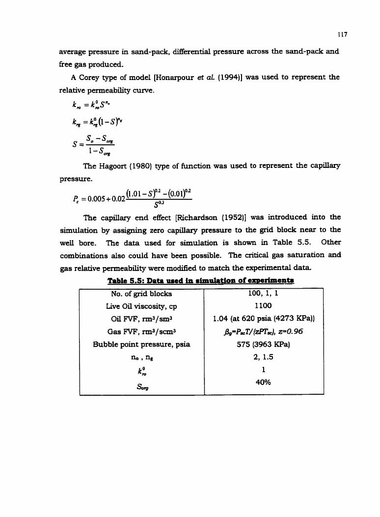
average pressure in sand-pack, differential pressure across the sand-pack and
fiee gas produced.
A Corey type of model [Honarpour et aL (1994)l was used to represent the
relative permeability curve.
The Hagoort (1980) type of function was used to represent the capillary
pressure.
The capillary end effect (Richardson (1952)l was introduced into the
simulation by assigning zero capillary pressure to the grid block near to the
w d bore. The data used for simulation is shown in Table 5.5. Other
combinations also could have been possible. The critical gas saturation and
gas relative permeability were modified to match the experimental data
Table 5.5: Data used in simulation of experiments
No. of grid blocks
Live Oil viscosity, cp
Oil FVF, rm3/smJ
Gas FVF, rm3/scmJ
Bubble point pressure, psia
n, , ng
kll,
s,
LOO, 1, 1
1100
1.04 (at 620 psia (4273 KPa))
J g = P r T / ( f l ~ ) , PO. 96
575 (3963 m a )
2, 1.5
1
40%

5.7.2 Analysis of the results
The match for the simulated run with the experimental data is shown in
Figures 5.16 - 5.18 and 5.2 1 - 5.22. Figure 5.16 shows the simulated data of
average pressure in the core. The initial and the later part of the data match
quite well. The non-equilibrium data cannot be matched as the simulator nlns
on equilibrium assumption.
Figure 5.17 and 5.18 matches the differential pressure data. The dip in
the differential pressure in all the cases is an indication of gas being formed at
outlet end, whereas there is stiU single-phase at the no flow boundary. This
results in sudden decrease of differentid pressure. This effect had been
discussed earlier in the chapter. This behaviour in the simulation run at early
time is shown in Figure 5.23, where the production-end pressure and no-flow
boundary pressure is plotted for Run 4. The change in slope of the lines occurs
at the different depletion volumes, which correspond to bubble point pressure.
This results in drop in the differential pressure in the sand-pack. This
phenomenon happens in the simulator at the bubble-point, since equilibrium
assumption is considered in a simulator. This does not match with the
experimental results where the bubbles nucleate after achieving a certain
supersaturation. For example, in Figure 5.18 for Run 4, this happens at AV=
0.7 cc for simulation run and at bV= 2.4 cc for experimental run. Beyond this
point, the experimental data matches quite well with the simulated results. A
discrepancy is obsenred in Run 3 (0.37 cc/hr) where, near AV=14 cc the
differential experimental pressure drops whereas in the simulation results it
increases slightly. This may be due to coalescence/movement of gas inside the
sand-pack. Once critical gas saturation is reached and the gas production
starts, the simulated results match the experimental data well again.
Figure 5.21 shows the match of gas saturation in the sand-pack
Actually, this was the data, which was matched on the simulator to determine
the reIative permeability values. As is evident, a very satisfactory match has
been obtained,
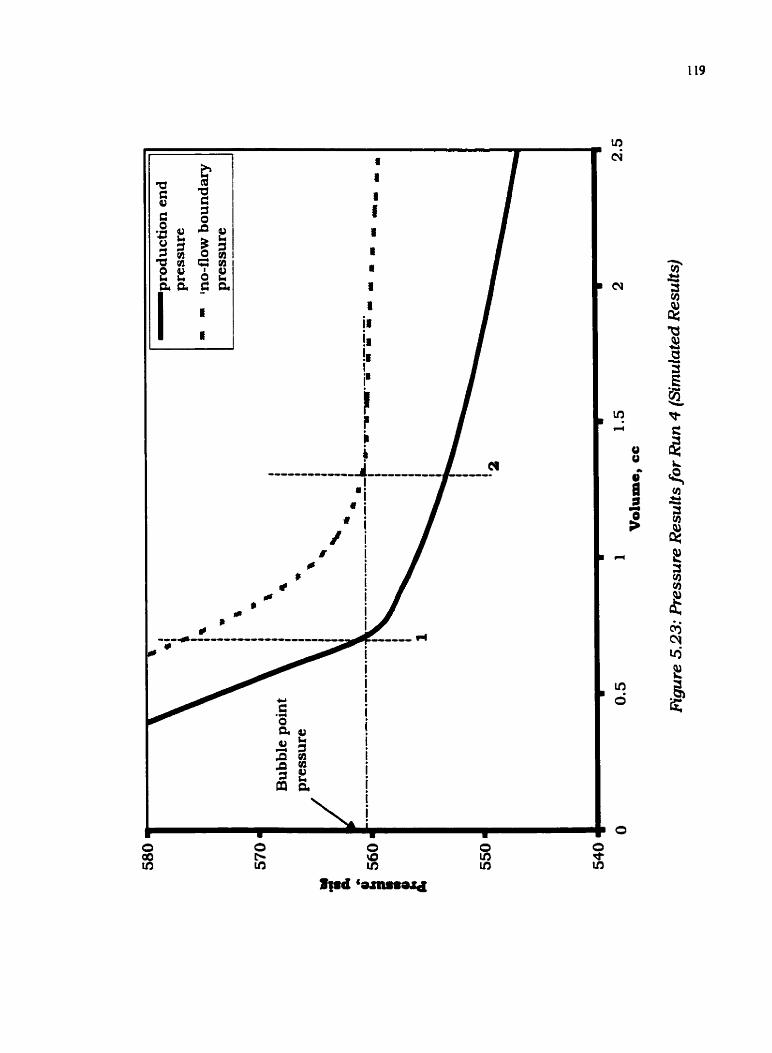

The fkee gas produced is compared in Figure 5.22. A relatively
satisfactory match is obtained for Run 1 and 3 (0.08 and 0.37 cc/h.). The
match is not quite good for Run 4 (3 cc/hr), where the values vary slightly at
higher production volumes. The simulation results do not match satisfactorily
for Run 6 (12 cc/hr). Things are happening so fast that the system is not able
to reach equilibrium (evident from Figure 5-16), so the fkee gas is expected to
be less than the equilibrium value. Since the simulator runs on equilibrium
assumption it is expected that it cannot model faster experiments which is
dominated by non-equitibrium effects.
Figure 5.24 shows the gas relative permeability obtained from
simulation. The shifting of curves downward with increasing depletion rate
indicates that the relative permeabilie of gas decreases with increase in
depletion rate. A shift in the curves to the right with increasing depletion rate
connotes increase in critical gas saturation with depletion rate.
The gas relative permeability values fkom our runs is compared with that
in light and heavy oil obtained from experiments of Pooladi-Danish and
Firoozabadi (1999). It can be seen that relative permeability for Run 1 and 6 is
about 2.5 and 4 orders of magnitude lower than that in light oil. Here we have
conhned the previous obsemation [Pooladi-Darvish and Firoozabadi (1999)],
that gas relative permeability in heavy oil is very low.
The depletion rate of the heavy oil run of Pooladi-Darvish and
Firoozabadi (1999) is similar to our Run 1, i.e. about 1 pore volume every 2.5
days. The viscosity of the oil used in their runs was 38,000 cp. whereas for our
runs it was 1100 cp. Comparing Run 1 with the heavy oil run of Pooladi-
Darvish and Firoozabadi (1999) shows the effect of viscosity on gas relative
permeability (see Figure 5.24). The gas relative permeability seems to be
lowered significantly (about 2 and 4 orders of magnitude for 1100 and 38,000
cp oil, respectively) with increase in viscosity of oil. F'urther studies need to be
done to ascertain the exact nature of effect of viscosity on gas relative
permeability.

Figure 5.24: Gas Relative Permeability
1 ,E-0 1
1,E-02 I
1.E-03 I
l.E-04 a
1iEa05 9
V W ---- e-
rrrr-
m-H"-
r e r Z #
c@ 4
" I . . I . C - - ' r~ 0 - Run1 ,,,I.-- - - - - ' ' ,. ---'Run3,, --- - - - -
. I- #,"--- - = = - 0.08 cc/hr (Run 1) - -0.37cc/hr (Run 3)
W e +- --L
Run 4
Run 6 - I - - '
rrp- w--
@--
1.E-06
-3 cc/hr (Run 4)
- 12 ccfhr (Run 6) - - Light Oil, Ref. (1999) - rn Heavy Oil, Ref* (1999)
1.E-07 -, 1 m I m ¤
0.00 0.02 0.04 0.06 0.08 0.10 0,12 QM Saturation

Single phase Preuure drop, psi/hr 0 200 400 600 800 1000
0 2 4 8 10 12 14 P Dep etion rate, cc/hr
Rgure 5.25: Critical Gas Saturation vs. Depletion Rate

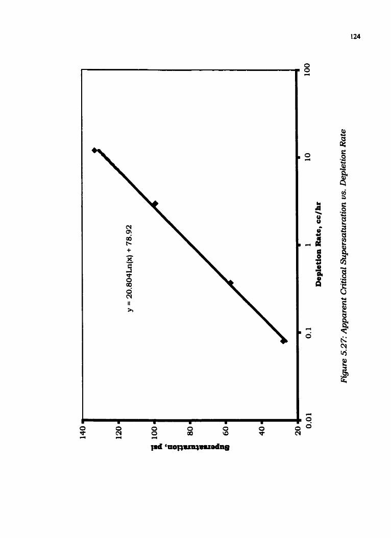

Considering the results of gas relative permeability in light of all the
experimental observations and results, conclusion can be drawn that increase
in depletion rate decreases the gas relative permeability, results in lower kee
gas production and higher gas saturation in sand-pack. The higher depletion
rate was also observed to result in fluid production with more entrained and
dispersed gas. Studies [Falls (1988)l have shown that more dispersed gas flow
reduces the gas relative permeability. Hence, this could be one of the factors
contributing to lower gas phase mobility.
In Figure 5.25 Critical Gas Saturation, as obtained from the simulation,
is plotted against depletion rate. Although the average gas saturation in the
sand-pack for all the runs, when the critical gas saturation is reached, is 3-4%,
it was found that to match the experimental results, the critical gas saturation
had to be significantly increased for the faster depletion runs. This is because
a saturation gradient exists along the sand-pack due to high pressure gradient
in faster depletion runs. Higher gas saturation at the outlet end, at hi*
depletion rates, has been observed in some of the previous works [Sarma and
Maini (1992)j. A critical gas saturation of 3% was obtained for Run 1 (0.08
cc/ht.), whereas a critical gas saturation of 7% was obtained for R u n 6 (12
cc/hr). A straight line can be fitted through the data.
Figure 5.26 shows the effect of depletion rate on K:; the end point
value of gas relative permeability. A semi-log model can be fitted into the
experimental data.
In Figure 5.27 "Apparent Critical Supersaturation" is plotted against
depletion rate. Here again a semi-1og model can be developed to predict
"Apparent Criticai Supersaturation".
Correlations developed in Figures 5.25 - 5.27 are only applicable for the
system under study and depend on the choice of our model (Corey model).
They indicate the trend observed by the parameter due to change in depletion
rate. The coefficients of the model may not be suitable to predict the parameta
in 0th- systems, since the values of the parameter might depend on a number
of factors other than depletion rate e.g. viscosity, porous media, oil type etc. A


detailed study needs to be done, considering all the factors, to develop a
comprehensive model, which can predict these parameters for any system, and
examine the applicability of semi-log and b e a r relationships, suggested here.
Recently, in a similar study [Guo-Quig and Firoozabadi (1999)] the
relative permeability was calculated based on Darcy's law. The analysis
considered negligible saturation gradient across the core. This may be true for
the case where there is negligible pressure drop across the sand-pack. This
approach is not applicable for Runs 3, 4 and 6 since there is considerable
pressure drop across the sand-pack which results in a saturation gradient.
However, this analysis can be applied for Run 1 where there is negligible
pressure drop across the sand-pack.
Figure 5.28 shows the comparison of gas and oil relative permeability
values as obtained from caidation [Guo-Quig and Firoozabadi (1999)j with the
one generated using the Corey model used in the simulation of experiments. A
fair match could be obtained.
Experiments were carried out to investigate the factors leading to favourable
behaviour in heavy oil reservoirs under solution gas drive. muther, the
effect of rate of depletion on solution gas drive process was also studkd.
The obsewations from the experiments indicated that:
Average gas saturation in the sand-pack increased with depletion rate.
hence the produced fiee gas volume decreased.
Oil phase mobility did not increase upon formation of gas bubbles.
Fluid, with more entrained dispersed gas phase, was produced as the
depletion rate was increased.
It was dearly observed in the faster depletion runs, that the gas
nucleation point did not coincide with "Critical Supersaturation".

Higher depletion rate resulted in higher "Apparent Critical
Supersaturation"
After the runs were terminated the non-e@"brium eflects were absent
in the slower depletion rate runs but in the faster depletion rate runs the
non-equilibrium effects were still present.
2. The experiment was successfully simulated on Edipse-100 Black oil
simulator. AU the data were matched satisfactorily. The results from the
simulation indicate that:
The critical gas saturation was not very high (3-7%)
Gas phase relative permeability decreases with increase in depletion rate.
The gas relative permeabilie in heavy oil under study was low (10-6 to lo4,
depending upon depletion rate) for gas saturation upto 12%.
Critical gas saturation was observed to vary linearly with depletion rate.
A semi-log empirical model was developed to predict "Apparent Critical
Supersaturation" and end point with depletion rate for the system studied.

Chapter 6
A study on the bubble growth and gas mobility measurement in heavy oil
was done. The following main findings were made from the study:
1. From the bubble growth study it was found that hydrodynamic forces do not
play a major role in bubble growth at late times and diffusion forces alone
may be adequate for modelling gas phase growth. It was found that a single
value of coefficients 'a' and 'b', in the growth model a t b , may not be valid at
all times; especially at early time. huther, the coefficients differ for infinite
and no-flow boundary growth cases. The subsequent modelling of the
constant volumetric rate depletion process in a dosed system, showed that
the nucleation of bubbles may not coincide with lowest point on the P-V
graph. In all the earlier studies, it was assumed that the bubbles nucleate
at the lowest point on the P-V graph. In the present study, it was found that
system pressure might fall even after nucleation of bubbles. A new term
"Apparent Critical Supersaturation" was defined for lowest point on the P-V
graph which was formerly termed as "Critical Supersaturation"; i-e. the
supersaturation at which the bubbles nudcate. Sensitivity studies
explained reasons for observance of different behaviour of heavy and light oil
systems.
2. The experiments, to measure the gas relative permeability in heavy oil and
study the effect of depletion rate on the solution-gas drive process were
conducted successfuly. The results indicated that the gas phase relative
permeability is much lown in heav oil, as compared to that in light oiL The

effect of some of the other theories, postulated to explain the favourable
behaviour of heavy oil reservoirs, was not found to exist in the current
experiments. The gas phase relative permeability was found to decrease
with increase in depletion rate. The critical gas saturation and
supersaturation were observed to increase with depletion rate. Low gas
phase relative permeability, was presented as one of the reasons
contributing to favourable behaviour of heavy oil reservoirs.
6.2. Recommendations
The present study does not resolve all the issues related to the
favourable behaviour of heavy oil resemoirs. It is just a small contribution to
explain the complex phenomenon. A lot of work still needs to be done, to
address al l the aspects. Some of the work recommended for future, which shall
compliment the present study, is as follows:
1. The capillary forces term (incorporating the effect of porous media) needs to
be included in the bubble growth model. Comprehensive modelling of gas
phase growth in porous media may require network modelling.
2. The effect of oil viscosity on the solution-gas drive process needs to be
explored more thoroughly. The proposed study should include observing
various parameters that are affected by the change in oil viscosity. The
results from this proposed study along with the results from the current
study will help in developing a model to predict gas phase relative
permeability as a function of viscosity and depletion rate.
3. Since the formation of 'Ifbamy oilw is debatable under slow depletion
experiments, experiments should be done with sand production, thus
simulating formation of t'wormholes". The existence of high pressure
gradient and formation of 'pamy oil" should be observed in such
experiments. Once again, scaled experiments simulating the field operating
conditions should be performed. The results &om these experiments shall
confirm presence of "jimmy oil'.

4. Last but not the least, results fkom comprehensive studies on phenomenon
such as supersaturation, nucleation, coalescence, sand-production,
rheology, thermodynamics and £low need to be assimilated, to present a
model to explain favourable behaviour of heavy oil reservoirs.

REFERENCES
AEUB: "Alberta's Energy Resources-1996 in Review", Alberta Energy and
Utilities Board, (1997) 6-7.
HEPTER, L. G., and HIS, C., AOSTRA Technical Handbook on Oil Sands,
Bitumen and Heavy Oil; AOSTRA Technical Publication Series # 6, 1989.
BAIL, P. T. and MARSDEN, S. S., Saturation Distribution in a Linear System
During Oil Displacement; Producers Monthly, pp. 22-32, June 1957.
BATYCKY, J. P., LEAUTE, R. P., and DAWE, B. A., A mechanistic model of
Cydic Steam Stimulation, paper SPE 37550; Resented at the International
Thermal Operations and Heavy Oil Symposium, Bakersfield, CA, Feb 10- 12,
1997.
BENTSEN, R. G., Conditions Under which the Capillary Term may be Neglected,
Journal of Canadian Petroleum Technology, pp. 25-30, Oct-Nov 1978, Montreal.
BORA, R., Cold Production of Heavy Oil - A n Experimental Investigation of
Foamy Oil Flow in Porous Media; Ph.D. Dissertation, University of Calgary,
1998.
BORA, R. and MAINI, B. B., Flow Visualisation Studies of Solution Gas Drive
Rocess In Heavy Oil Reservoirs Using a Glass Micromodel; SPE 37519
Resented at the SPE International Thermal Operations and Heavy Oil
Symposium, Bakersfield, CA, Feb. 10-12, 1997.
BOYER, R L., MORGAN, F., and MUSKAT, M., A New Method for Measurement
of Oil Saturations in Core; TP 2 124 in Petroleum TechnoIogy, January 1947.

BRENNEN, C. E., Cavitation curd Bubble Dzjnamics; Oxford University Press,
1995.
BUTLER, R. M., Thermal Recovery of Oil and Bitumen; RenticeHall kc., 199 1.
CARMAN. P.C., Fluid Flow Through Granular Beds. Trans. Inst. C h e m Eng.,
Val. 15, 150-166, 1937.
CHARDAIRE, C., Simultaneous Estimation of Relative Penneabilities and
Capillary Pressures; presented at the 64th Annual Technical Conference and
Exhi'bition of the SPE held in San Antonio, TX, October 8- 1 1, 1989.
CIVAN, F, and DONALDSON, E. C., Relative Permeabilie fkom Unsteady-State
Displacements: An Analytical Interpretation; SPE 16200, presented at the SPE
Production Operations Symposium held in Oklahoma city, Oklahoma, March 8-
10, 1987.
CLARIDGE, E. L. and FRATS, M., A Roposed Model and Mechanism for
Anomalous Foamy Heavy Oil Behaviour; SPE 29243 Resented at the
International Heavy Oil Symposium held in Calgary, AB, Canada, June 19-2 1,
1995.
COLES, R., "Boiling Nudeation"; Advanced Heat Itatzsfer, 10, pp. 24-26, 1974.
CRAFT, B. C., and HAWKXNS, M. F., Applied Petroleum Reservoir Engineering;
Rentice Hall hc., 19
CRUM, L., Nucleation and Stabilization of Microbubbles in Liquids; Applied
Saentiflc Research. 38, pp. 10 1-1 15, 1982.

DANESH, A,, PEDEN, J. M., KRINIS, D., and HENDERSON, D., Pore Level
Investigation of Oil Recovery by Solution Gas Drive and Gas Injection; SPE
16956, presented at the 62 Annual Technical Conference and Exhibition,
Dallas, TX, September 27-30, 1987.
DUMORE, J. M., Development of Gas-Saturation During Solution-Gas Drive in
a n Oil Layer Below a Gas Cap; Society of Petroleum Engineers Journal, pp. 2 11-
2 18, September 1970.
DUSSEAULT, M., Cold Roduction and Enhanced Oil Recovery; Journal of
Canadian Petroleum Technology, pp. 16- 18, November 1993.
ECLIPSE 100 Reference Manual; Version 96A, Schhunberger, GeoQuest.
FALLS, D. H., HIRASAKI, G. J., PATZEK, T. W., GAGLXTZ, D. A., MILLER, D. D.
and RATULOWSKI, T., Development of a Mechanistic Foam Simulator:
Population Balance and Generation by Snap-otf; SPE Reservoir Engineering, pp
884-892, 1988.
FATT, J. and DYKSTRA, H., Relative Permeability Studies; Trans AIME, Val.
192, pp. 249 - 256, 1951.
FIROOZABADI, A*, and KASHCHIEV, D., Ressure and Volume Evolution
During Gas Phase Formation in Solution Gas Drive Rocess; Sodety of
Petroleum Engineers Journal, pp. 2 19-227, September, 1996.
FIROOZABADI, A., OTTENSEN, B., and MIKKELSEN, M., Measwments of
Supersaturation and Critical Gas Saturation; SPE Formation Evclhcation, pp.
337-344, December 1992.

GEFFEN, T. M., and GLADFELTER, R. E., A Note on the X-Ray absorption
Method of Determining Fluid Saturations in Cores; Tmns AIME, Vol. 195, pp.
322-323, 1952.
GEILKMAN, M. B., DUSSEAULT, M. B., and DULWEN, F. A. L., Dynamic
Effects of Foamy Fluid Flow In Sand Production Instability; SPE 30251
Presented at the International Heavy Oil Symposium held in Calgary, AB,
Canada, June 19-21, 1995.
GUO-QUIG, TANG., and FIROOZABADI, A*, Gas and Liquid Phase Relative
Permeabilities for Cold Production from Heavy Oil; SPE 56540 Resented at the
SPE Annual Technical Conference and Exhibition, Houston, TX, 3-6 October
1999.
HAGOORT, J., Oil Recovery by Gravity Drainage; Society of Petroleum Engineers
Jownaf, pp. 139-150, June 1980.
HANDY, L. L., A Laboratory Study of Oil Recovery by Solution Gas Drive; Rams
AIME, Vol. 2 13, pp. 3 10-3 15, 1958.
HELSET, H. M., NORDTVEDT, J. E., SKJOEVELAND, S. M., and VIRNOVSKY,
G. A., Relative Permeabilities from Displacement Experiments with Full Account
for Capillary Ressure; SPE Resemir Engineering curd Evahrotion, pp. 92-98,
April 1998.
HEMMINGSEN, E. A*, Cavitation in Gas-Saturated Solutions; Journal of Applied
Physics, 46,1, January 1975.
HOFFMAN, J. D., Numerfcul Methods for Engheers and Scientists; McGraw Hill
kc., 1992.

HOLM, L. W., The Mechanism of Gas and Liquid Flow Through Porous Media in
Resence of Foam; Society of Petroleum Engineers Journal, pp. 359-369,
December 1968.
HONARPOUR, M, KOEDERITZ, L., and HARVEY, A. H., Relative Penneabr'lity of
Petroleum R e s m i r s , Society of Petroleum Engineers hc. Publication, 1994.
HOYOS, M., MOULU, J. C., DEFLANDRE, F., and LENORMAND, R., Ultrasonic
Measurements of the Bubble Nucleation Rate During Depletion Experiments in
a Rock Sample; SPE 20525, presented at the 65" Annual Technical Conference
and Exhibition of the SPE held in New Orleans, LA, September 23-26, 1990.
HUANG, W. S., MARCUM, B. E., CHASE, M. R., and YU, C. L, Cold Production
of Heavy Oil from Horizontal Wells in the Frog Lake Field; SPE 37545, Resented
at the SPE International thermal Operations and heavy Oil Symposium,
Bakersfidd, CA, 10-12 February, 1997.
KUERTA, M., TICO, A., JIMENEZ, I., MIRABAL, M. DE., and ROJAS, G.,
Understanding Foamy Oil Mechanism for Heavy Oil Reservoirs During Rimary
Roduction; SPE 36749, Resented at the 1996 SPE Annual Technical
Conference and Exhibition, Denver, CO, October 6-9, 1996.
HUNT, E. B., and BERRY, V. J., Evolution of Gas From Liquid Flowing Through
Porous Media; MChE Journal, Vol. 2, No. 4, pp. 560-567, 1956.
ISLAM, M. R and CHAKMA, A*, Mechanics of Bubble Flow in Heavy Oil
Resemoirs; SPE 20070 Resented at the 60th California Regional Meeting,
Ventura, CA, April 4-6, 1990.

ISLAM, M. R, and PADDOCK, J., A New Equation of State for Crude Oils with
Microbubbles; 9943, presented at the CSPG and Petroleum Society Joint
Convention, Calgary, AB, June 14- 18,1999.
JOHNSON, E. F., BOSSLER, D. P., and NAUMANN, V. O., Calculation of
Relative Permeability from Displacement Experiments; Tmns AZME, Vol. 216,
pp. 370-372, 1959.
JONES, S. F., EVANS, G. M., and GALVIN, K. P., Bubble Nudeation form Gas
Cavities - A Review; Advances in Colloid and Iterface Science, 80, pp. 27-50,
1999.
KALAYDJIAN, F. J. M., Dynamic Capillary Ressure Curve for Water/Oil
Displacement in Porous Media: Theory Vs. Experiment; SPE 248 13, presented
at the 67th Annual Technical Conference and Exhibition of the SPE held in
Washington, DC, October 4-7, 1992.
KAMATH, J., and BOYER, R. E., Critical Gas Saturation and Supersaturation in
Low-Permeability Rocks; SPE 26663, SPE Formation Evatuation, pp 247-253,
December 1995.
KASHCHIEV, D., and FIROOZABADI, A., Kinetics of Initial Stage of Isothermal
Gas Phase Formation; J of C h e m Phys., 98,6, pp. 4690-4699, March 5, 1993.
KENNEDY, H. T., and OLSON, C. R., Bubble Fonnation in Supersaturated
Hydrocarbon Mixtures; naris AIME, Vol. 195, pp. 271-278, 1952.
KOVSCEK, A. R., and RADKE, C., Fundamentals of Foam Transport in Porous
Media; chapter 3 of "Foams: Fundamental and AppIication in the Petroleum
Industry", Schramm, L. L., Ed.; Advances in Chemktry Series 242, American
Chemical Soaetg, Wrshington D. C., 1994.

KRAUS, W- P., McCAFFFtEY, W. J., and BOYD, G. W., Pseudo-Bubble Point
Model for Foamy Oils; presented at the Annual Technical Conference of The
Petroleum Society of CIM, Calgary, AB, May 9-12, 1993.
LABTECH, LTseJs Guide, Laboratory Technologies Corporation; 1994.
LAIRD, A. D. K. and PUTNAM, J. A., Fluid Saturation in Porous Media by X-Ray
Techniques; Trans AIME, Vol. 192, pp. 275-284, 195 1.
LAIRD, A. D. K. and PUTNAM, J. A., Three Component Saturation in Porous
Media by X-Ray Techniques; Trans AIME, Voi. 2 16, pp. 2 16-220. 1959.
LEAS, W. J., JENKS, L. H., and RUSSEL, CHARLES. D., Relative Permeability
to Gas; Tmns AIME, VoI. 189, pp. 65-72, 1950.
LEVEREXT, M.C., Flow of Oil Water Mixture Through Unconsolidated Sands;
Rans AIME, Vol. 132, 149, 1939.
L E V E m , M.C., Capillary Behaviour in Porous Solids; Trans AIME, Vol. 142,
152-169, 1941,
LI, X. and YORTSOS, Y. C., Theory of Multiple Bubble Growth in Porous Media
by Solute Diffusion; C h e m Engg. Sfi, Vol. 50, pp. 1247- 1271, 1995.
LOUGHEAD, D. J. and SALTUKLAROGLU, M., LIoydminster Heavy Oil
Roduction - Why so Unusual?; Ninth Annual Heavy Oil Sands TechnoIogy
Symposium, Calgary, March 1 1, 1992.
MAIM, B. B., Foamy Oil Flow in Rimary Roduction of Heavy Oil under
Solution Gas Drive; SPE 56541, presented at the SPE Annual Technical
Conference and Exhibition, Houston, TX, 3-6 October, 1999.

MAINI, B. B., Laboratory Evaluation of Solution Gas Drive Recovery Factors in
Foamy Heavy Oil Resewoirs; presented at the CSPG and Petroleum Society
Joint Convention, Calgary, AB, 14- 18 June, 1999.
MAINI, B. B., Foamy Oil Flow in Heavy Oil Roduction; Journal of Canadian
Petroleum Technology, pp. 21-24, June 1996.
MAINI. B. B., Is it Futile to Measure Relative Permeabiliw for Heavy Oil
Reservoirs; Resented at the 46th Annual Technical Meeting of the Petroleum
Society of CIM, Banff, AB, Canada, May 14- 17,1995.
MAINI, B. B., SARMA, H. K., and GEORGE, A. E., Significance of Foamy-oil
Behaviour in Primary Roduction of Heavy Oils; Journal of Canadian Petroleum
Technology, pp. 50-54, November 1993.
McCABE, SMITH and HARRIOT; Unit Operations in Chemical Engineering;
McGraw Hill Publication, 1990.
METWALLY, M. and SOLANKI, S. C., Heavy Oil Reservoir Mechanisms,
Lindbergh and Frog Lake Fields, Alberta Part I: Field Observations and
Reservoir Simulation; presented at the 46th Annual Techaical Meeting of the
Petroleum Society of CIM, Banff, AB, Canada, May 14-17, 1995.
MIRABAL, M. DE., RODRIGUEZ, H,, and GORDIUO, R-, Impact of Foamy Oil
Mechanism on the Hamaca Oil Reserves, Orinoco Belt - Venezuela., SPE 36 140,
Resentcd at the Fourth Latin American and Caribbean Petroleum Engineexkg
Conference, Port of Spain, Trinidad and Tobago, 23-26 April 1996.
MIRABAL, M. DE,, RODRIGUEZ, HI, and GORDLLO, R., Production
Improvement Strategy for Fomy Hamaca Crude Oil; SPE 37544, Resented at

the SPE International Thermal Operations and Heavy Oil Symposium,
Bakersfield, CA, 10- 12 February, 1997.
MORGAN, F., McD07NEU. J. M., and DOTY, E. C., Improvements in the X-Ray
Saturation Techniques of Studying Fluid Flow, Trans AXME, Vol. 189, pp. 183-
194, 1950.
MOULU, J. C., Solution-Gas Drive: Experiments and Simulation; Jacmaf of
Petroleum Science and Engineering, 2, pp. 379-386, 1989.
MUSKAT, M., Physical Rinciples of Oil Production, McGraw-Hill Book Co., N.Y.,
1949.
OAK, M. J., BAKER, L. E. and THOMAS, D. C., Three Phase Relative
Permeability of Berea Sandstone; Journal of Petroleum Technology, pp. 1054-
106 1, August 1990.
OAK, M. J. and EHRLICH, R., A New X-Ray Absorption Method for
Measurement of Three Phase Relative Permeability; SPE Resemoir Engineering,
pp. 199-206, February 1998.
ODEH, A. S., Effect of Viscosity Ratio on Relative Permeability; Trans AIME, Vol.
216, PP. 346-353, 1959.
OSOBA, J. S., RICHARDSON, J. G,, KERVER, J. K, HAFFORD, J. A., and
BLAIR, P. M., Lab Measurement of Relative Permeability; k n s AIME, Vol. 192,
pp. 47-56, 1951-
PARSONS, R W., Miaowave Attenuation - A New Tool for Monitoring
Saturations in Laboratory Flooding Experiments; Society of Petroleum Engineers
J ~ u n ~ r t , pp. 302-3 10, August 1975.

PATEL, R. D., Bubble Growth in Viscous Newtonian Liquid; C h e m Engg- Sd,
Vol. 35, pp. 2352-2356, 1980.
POOLADI-DARVISH, M. and FIROOZABADI, A., Solution Gas Drive in Heavy Oil
Reservoirs; Journal of Canadian Petroleum Technology, pp. 54-6 1 ,April 1999.
POON, D., and KISMAN, K., Non-Newtonian Effects on the Primary Production
of Heavy Oil Reservoirs; Jaumal of Canadian Petroleum Technology, pp. 55-59,
September 1992.
RAMEY, H. J., Rapid Methods for Estimating Reservoir Compressibilities;
Journal of Petroleum Technology, pp. 447454, April 1964.
RAPOPORT, L. A., and LEAS, W. J., Relative Permeabiliv to Liquid in Liquid
Gas Systems; Trans AIME, Vol. 192, pp. 83 - 98, 1951.
RICHARDSON, J. G., KERVER, J. IC, HAFFORD, J. A., and OSABA, J. S.,
Laboratory Determination of Relative Permeability; Trans AIME, Vol. 195, pp.
187-196, 1952.
ROSE, W., Theoretical Generalizations Leading to the Evaluation of Relative
Permeability; Trans. AIME, pp. 1 1 1- 126, 1949.
ROSNER, D. E. and EPSTEIN, M., Effect of Interface Kinetics, Capillarity and
Solute Diffusion on Bubble Growth Rates in Highly Supersaturated Liquids;
Chem. Engg. Sd, Vol. 27, pp. 69-88, 1972.
SARMA, H. K., and BENTSEN, R. G., A New Method for Estimating Relative
Permeabilities from Unstabilised Displacement Data; Journal of Canadian
Petroleum Technology, Vol. 28, No. 4, pp. 118-128, JuIy-Aug 1989.

SARMA, H. K., and BENTSEN, R. G., Further Experimental Validation of the
External-Drive Technique; Jacmal of Canadian Petroleum Technology, Vol. 29,
NO. 4, pp. 75-83, July-Aug 1990,
SARMA, H., and MAINI, B., Role of Solution Gas in Rimary Roduction of Heavy
Oils; SPE 23631, presented at the Second Latin American Petroleum
Engineering Conference, Caracas, Venezuela, March 8- 1 1. 1992.
SCRIVEN, L. E., On the Dynamics of Phase Growth; Chem Engg. Sci.. Vol. 10,
pp. 1-13, 1959.
SHEN, C. and BATYCKY, J., Some Observations of Mobility Enhancement of
Heavy Oils Flowing Through Sand Pack Under Solution Gas Drive; Journal of
Canadian Petroleum Technology, pp. 46-53, April 1999.
SHENG, J. J., MAINI, B. B., HAYES, R. E., and TORTIKE, W. S., Experimental
Study of Foamy Oil Stability; Jacmal of Canadian Petroleum Technology, pp- 3 1-
37, April 1997.
SHENG, J. J., HAYES, R E., MAIM, B. B., and TORTIKE, W. S., Modelling
Foamy Oil Flow in porous Media; Tmnsport in P o m s Media, 35, pp. 227-258,
1999.
SHENG, J. J., HAYES, R. E., MAIM, B. B., and TO-, W. S , A Non
E@'brium Model to Catdate Foamy Oil Properties; Jaumal of Canadian
Petroleum Technology, pp. 3845 , April 1999.
SMITH, G. E., Fluid Flow and Sand Roduction in Heavy Oil Resewoh Under
Solution Gas Drive; SPE 15094, SPE hduction Engineering, pp 169-179, May
1988.

STEWART, C. R., CRAIG, F. F. Jr., and MORSE, R. A., Determination of
Limestone Performance Characteristic by Model Flow Tests; Trans AlME, Vol.
198, pp. 93-102, 1953.
STEWART, C. R., HUNT, E. B., SCHNEIDER, F. N., GEFFEN, T. M., and BERRY,
V. J., The Role of Bubble Formation in Oil Recovery by Solution Gas Drives in
Limestones; nuns AIME, Vol. 20 1, pp. 294, 1954.
SZEKELY, J. and MARTINS, G. P., Non EquiIibrium Effects in the Growth of
Spherical Gas Bubbles due to Solute Diffusion; Chem Engg. S k , Val. 26, pp.
147-159, 1971.
SZEKELX, J. and FANG, S. D., Non Equilibrium Effects in the Growth of
Spherical Gas Bubbles due to Solute Diffusion - 11; Chem. Engg. Sci., Vol. 28,
pp. 2 127-2 140, 1973.
TAXLER, R.N., and BAUM; L.A.H., Permeability of Compacted Powder - Determination of Average Pore size. Physics, 7, pp. 9 - 14, 1936.
TREMBLAY, B., SEDGWM, G.and W, D., CT Imaging of Sand Production in a
Horizontal Sand Pack Using Live Oil; Resented at the 49th Annual Technical
Meeting of The Petroleum Society in Calgary, AB, Canada, June 8- 10, 1998.
TREINEN, R. J., RING, W. W., SPENCE, A. P., MIRABAL, M. DE. and HUERTA,
M., Harnaca: Solution Gas Drive Recovery in Heavy Oil Reservoir, Experimental
Results; SPE 3903 1, Resented at the Fifth Latin American and Caribbean
Petroleum Engineering Confennce and Exhibition, Rio de Janeiro, Brazil,
August 30-September 3, 1997.

WALL, C. G., and KHURANA, A. K., The Effects of Rate of Pressure Decline and
Liquid Viscosity on Low-Pressure Gas Saturations in Porous Media; Journal of
the Itzstitute of Petroleum, pp. 335-345, November L972.
WARD, C. A., TMUISIS, P., and VENTER, R. D., Stability of Bubbles in Closed
Volume of Liquid-gas Solution; Journal of AppIied Physics, 53(9), pp. 6076-
6084, September 1982.
WARD, C. A., and LEVART, E., Conditions for Stability of Bubble Nuclei in Solid
Surface Contacting a liquid-gas Solution; Journal of Applied Physics, 56(2), pp.
49 1-500, July 1984.
WATSON, A. T., MCHMOND, P. C., KERIG, P. D., and TAO, T. M., A Regression-
Based Method for Estimating Relative Permeabilities From Displacement
Ekperiments; SPE Resemir Engineering, pp. 9 53-958, August 1988.
WILT, P. M., Nudeation Rates and Bubble StabiIity in Water-Carbon Dioxide
Solutions; Journal of Colloid and Interface Science, 1 12, 2, August 1986.
WONG, R. C. K., GUO, F., WEAVER, J. S., and BARR, W. E., Heavy Oil Flow
Under Solution-gas Drive: Pressure Depletion Tests; Journal of Canadian
Petroleum Technology, pp. 3 1-37, April 1999.
YOUSFI, A. El., ZARCONE, C., BORES, S., and LENORMAND, R., Physical
Mechanisms for Bubble Growth during Solution Gas Drive; SPE 38921.
presented at the Annual Technical Conference and Exhi'bition, San Antonio, m, October 5-8, 1997.
ZHANG, Y., Temperature Effects on Foamy Solution-Gas Drive; M. Sc. Thesis,
University of Calgary, 1999.

SOLUTION FOR BUBBLE GROWTH
AI. 1. Fornulation of the Problem
Consider a stationary spherical gas bubble in a quiescent supersaturated
liquid. It grows due to the transfer of a dilute component kom the supersaturated liquid to the gas (vapour) inside the bubble. The density and
viscosity of the liquid is assumed to be constant and the system isothermal. It
is assumed that thermodynamic equilibrium exists at the gas-liquid interface.
Figure AI: Schematic representation of the bubble growth system (Modified fiom
Szekw and Fang (1 973))
By using these assumptions, the equations of continuity and motion may
be combined in spherical co-ordinate system to obtain the following equation
for bubble growth [Brennen (1995)j (see Figure Al).
where, R is the bubble radius.

PL,Ris related to P,,, through the continuity of the normal stress on the
surface of the bubble. This relationship is expressed as (Brennen (1995)j
2 0 4pdR ----- PL.R=PG*R dl (1-2)
In Equation (I-2), the difference in pressure in the bubble and at its
surface is the driving force for growth and has to overcome the viscous
momentum transfer and the work done by surface tension forces. The above
two equations can be combined to give:
"R 3 ;,[ 2cr (dRldt) R--T+- - =- PG,R --- dt- 2 dt 4p R
For transfer of the solute from the liquid phase to the gas phase by
diffusion a mass conservation equation can be written in spherical co-ordinates
[Brennen (1995)j as:
where the above equation utilises the fact that:
- dR -- dR utId- dt and u r r 2 = R ' - dt
Next the initial and the boundary conditions are written. For initial
conditions spedfying an initial bubble size (Ro), zero initial growth rate, and
uniform solute distribution in the liquid we can write:
R = R,,, t = O
We assume bubble to be already nucleated and in thermodynamic and
physical equilibrium wi th the surrounding li@d, so an initial zero growth rate
is valid. Regarding the boundary conditions for the infinite case, we consider
concentration of solute far from the bubble remains constant:
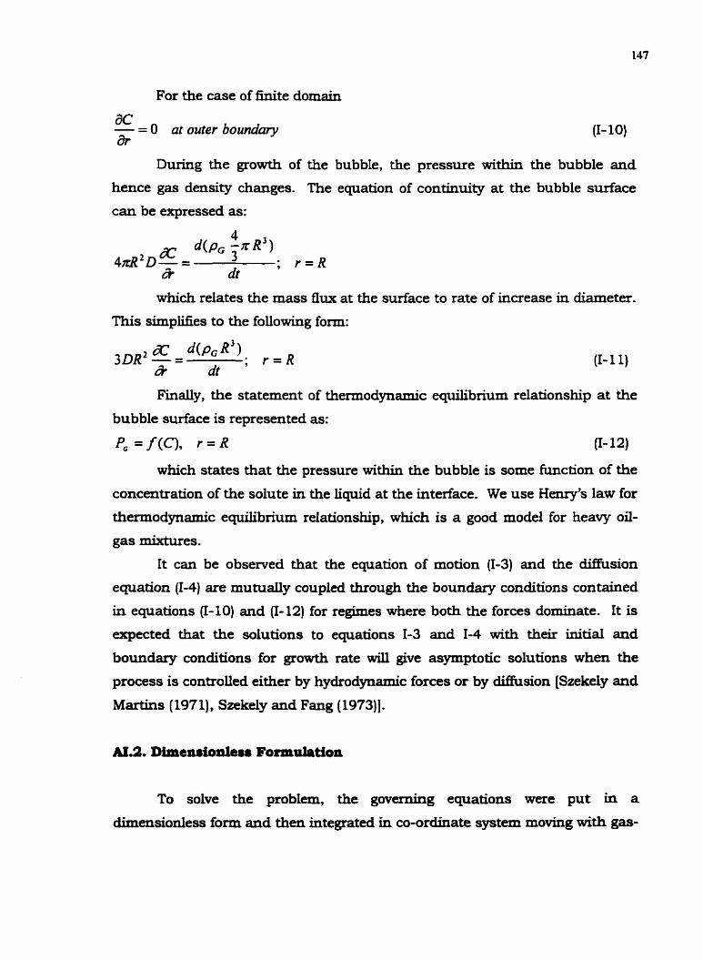
For the case of finite domain
ac - = 0 at outer boundary (1- 10) ar
During the growth of the bubble, the pressure within the bubble and
hence gas density changes. The eqyation of continuity at the bubble surface
can be expressed as:
which reIates the mass flux at the surface to rate of increase in diameter.
This simplifies to the following form:
(I- 1 1)
Finally, the statement of thermodynamic eqydibrium relationship at the
bubble surface is represented as:
(I- 12)
which states that the pressure within the bubble is some fiulction of the
concentration of the solute in the liquid at the interface. We use Henry's law for
thermodynamic equilibrium relationship, which is a good model for heavy oil-
gas mixtures.
It can be observed that the equation of motion (1-3) and the diffbsion
equation (1-4) are mutually coupled through the boundary conditions contained
in equations (I-10) and (1-12) for regimes where both the forces dominate. I t is
expected that the solutions to equations 1-3 and I 4 with their initid and
boundary conditions for growth rate will give asymptotic solutions when the
process is controlled either by hydrodynamic forces or by diffusion [Szekeiy and
Martins (197 I), Szekely and Fang (1973)l.
AI.2. Dimensionless Formulati on
To solve the problem, the governing eqyations were put in a
dimensionless form and then integrated in co-ordinate system moving with gas-

oil interface through the use of finite difference method. The dimensionless
parameters used are defined in Table 4- 1.
Application of dimensionless number into the model ecpations is given
below. Defining the derivatives of dimensionless parameters for incorporation
into equations results in:
(1- 13)
(1- 14)
(I- 15)
(I- 16)
11-17)
AI.2.l. Hy&odynamic Growth Model
In the process of conversion to dimensionless form, the hydrodynamic
equation (1-3) can be written as:
Substituting the dimensionless parameters from Table 4.1, derivatives
values from equations I- 13 to 1-17 and simplifying we get above the equation in
the foUowing form:
this huther can be simplified to

G 3 ( d 5 ) 2 + ~ % = G [ n - - ] - - [ p L s a ] g ~ + ~ dr (I- 18)
c d? 5 P o
Since, equation 1-18 is a non-linear equation it needs to be Zinearised
before being solved by finite difference method. Newton's linearisation method
is used for this purpose.
AI.2.2. Difhsion Growth Model
Since bubble growth is a moving boundary problem, a new set of co-
ordinates are defined that move with the bubble boundary. The new co-
ordinate is defined in Table - 4.1 and is represented by q . Below we define dimensionless terms, that are affected by moving
boundary, for diffusion equation:
Substituting value of derivatives from equation 1-13 to 1-17, the above
equation simplifies to,
(I- 19)
By substituting equation 1-19 and other dimensionless parameters into
equation 1-4, we get the following form of diffusion equation,
which simplifies to,

AI.2.3. Equilibrium at the intertpce
Henry's law is used to express equilibrium condition at the interface.
This is represented as:
fG = Kc, (1-2 1)
Where, Po is the pressure inside the bubble, C, is the interface solute
concentration and K is the H e w s constant. Writing the above correlation for
initial condition:
Po = KC, (1-22)
Dividing equation 1-2 1 by 1-22 we have the following expression
This is substituted in equation 1-18 to eliminate n from the equation.
c:, is the concentration at the interface and is also expressed as C; .
A1.2.4. Initial and Bouadaxy Conditions
(i) For hydrodynamic growth model
The initial conditions, 1-6 and 1-7, can be written in dimensionless form
as,
5=1 at r = O (T-24)
dz
The hydrodynamic model is solved with the above initial condition to
arrive at the bubble growth solution limited by hydrodynamic forces only.
(iiJ For d i m o n growth model
The initial and boundary conditions (1-8 and 1-9) in dimensionless form
can be written as,
~ ' ( 0 , ~ ) ' I (I-26)

For diffusional growth model it is assumed that there is no pressure
driving force (or PL , equals pressure in the bubble, P, ). So,
The above boundary conditions are solved with the initial condition 1-24
and 1-25 to arrive at the solution. The above formulation is valid for infinite
domain. For finite domain the boundary condition 1-27 changes. The
formulation for finite domain is given later.
(iii) For general growth model
The mass flux at the boundary is represented by equation I- 11. The gas
density is not assumed to be constant and changes with the change in
pressure. Equation I- 1 1 can be expanded a s follows:
MP, The ideal gas law is assumed. Thus, p, = - YT
Where, M is the molecular mass, y is the gas constant and T is the
temperature. Converting the above equation into dimensionless form by
applying dimensionless parameters, the equation can be written as:
Simplifying the above equation and substituting
in the equation, we end up with the following form of above equation,

In the general growth model, the hydrodynamic (I- 18) and diffixsion (1-20)
equation are solved along with initial condition 1-24 to 1-26, boundary condition
1-27 or 1-30 (as the case may be), 1-29 and equilibrium assumption (1-23).
(iv) Forfinite domain
The infinite source of solute condition (boundary condition 1-27) is no
more valid. Instead, the boundary condition equation 1-10 is applied at the far
boundary, that can be written in dimensionless form as:
This reflects that there is zero influx of solute at the fat boundary. The
far boundary is fixed and stationary, whereas the bubble interface is moving
outwards. This results in shrinkage of space between bubble interface and
fixed outer boundary. This can be viewed as inward movement of the far
boundary, as the bubble grows. This during simulation, translates into renewal
of number of grid blocks at each time step.
N.2.5. Conrtaat mate of prcs.9rr drop
A function is defined for pressure variation in the field with respect to
time, which is expressed as:
P,,, = 4 -ct (I-3 1)
Where, c is the rate of pressure drop. The above equation impIies that
pressure is dropping at a constant rate in the system. This is substituted in
equation 1-18 for P,, to get the sotution.

AI.2.6. Solmtion gas U v e model
Since a direct relation of pressure with time is not available for constant
volumetric rate depletion, the folIowing additional equation is solved along with
the above equations for solution:
Where, K, is the compressibili~ of oil. This is the compressibility
equation, that relates volume depleted to the pressure in the system. This in
difference form results in
Where, the subscript f denotes the resultant value and I, the value at
previous time step. 5 is given by
Wheze, B, and V, are number of bubbles and pore volume respectively.
The equation implies that final volume oil volume is equal to pore volume minus
the voiume of gas phase. Substituting equation 1-33 into 1-32 results in
The value of Pf is equivalent to PL,in equation 1-18. Equation 1-34
defines pressure in terms of radius of bubble and fluid withdrawn (known
value). Substituting this expression in equation I- 18 eliminates PL., and gives
equation 1-18 in terms of g.

L
Equation 1-35 is solved with equations 1-20, boundary conditions 1-23, I-
29, 1-30 or 1-27, and initial conditions 1-24, 1-25, 1-26 to obtain the solution for
constant volumetric rate depletion problem.
For constant pressure drop probelm, equation 1-31 is substituted for P',,
and the problem is solved similariy.
AIe3. Nunrerical Solution
For solution of the bubble growth problem, all the equations were put in
finite difterence form and solved numerically. Since the hydrodynamic and the
diffusional growth model equations are non-linear, they were linearised before
obtaining finite difference form.
Newton's method [Hohan , (1992)j was used for hearisation. This
involves guessing the value of the solution and substituting into the equation.
The solution is assumed to be represented as,
4" = 5; + 6" (1-36)
where subscript e denotes the estimated (guessed) value of the solution,
and i, the position in space. Superscript n is the time step number, in the
solution process. 8 and a are the errors in the guess value of the solution. The
errors are assumed to be very small. While linearising any second order term of
error is negIected in the equation, and hence we obtain a linearised eqyation for
solution. So now, since the solution is guessed, the linear equation is solved for
the errors instead of &owns. The solution for unknowns is arrived at, by
substituting errors into equation 1-36 and 1-37.

The following equations for derivatives can be obtained from above
equations
d 2 ~ " d'g: d26" -=- +- dr' dr2 dr2
cc i3C:;,n aa: -=-+- a? a7 all
AI.3.1. Finite Mfterence form of Dimensionless Equations
All the dimensionless equations are put in h i t e difference form, to
obtain a set of linear algebraic equations that are then put into a matrix and
solved simultaneously at a particular time step. An LU decomposition method
is used to solve the equation. An implicit method is used while writing the
equation in finite difference form, thus eliminating stability problem in the
solution.
Backward Time Centred Space (BTCS) method is used while discretising
the equations. The finite difEerence form of the derivatives of 6, a, 5: and c:: is
Since the solution at prewious time is known, the errors for previous time
steps are assumed to be zro. So the above equations can be written as

d28" 6" -- -- d?' ~r~
Similarly,
for derivative of the space co-ordinate
aa: - - a:,, +a:, and all 2Arl
Similarly, the guessed (known) quantities are put into finite difference
form as follows:
' f2gn ,g;-2g-'+g:-' L= ds' A ? ~
AK.3.1.1. Hydrodynamic growth equation
For Solution Gas Drive Model
Equations 1-36 to 1-39 are substituted into 1-35. The higher order terms
of S are neglected to make the final equation hear wi th respect to the errors.

Finally, the finite difference approximation equations 1-43 and 1-44 are
substituted into the equation to get the following form:
(1-53)
The tenns in parenthesis on the LHS and all the terms on RHS are
known values. The derivative values are calculated from equations 1-48 and I-
49 at each time step. The known values in the above eqyation 1-53? can be
represented by constants resulting in linear form of equation 1-5 1, written as:
arsn -Gar = 6," (1-54)
As mentioned previously, for constant pressure decline model, equation
E3 1 is substituted into equation I- 18 and a similar procedure as stated above is
followed to get the bite difference form. The values of the constants change
but the form of the linear equation is the same as 1-54.
AI.3.1.2. DiaRuive growth equation
Equations 1-36 to 1-38? and 1-40 to 1-42 are substituted into equation I-
20 and the higher order terms of Gand a are neglected to obtain the b e a r form
of diffusion equation. Ekther the finite difference approximation from equation
1-43? I45 to 1-48, 1-50 to 1-52 are applied to get the following simplified form of
diffusion equation.
where,

* - (1 - ) -- a a;,, 2- dgn ac;; - Qtzi - ac:;
AT a? d7 aq 4 . i - a rl
Further, the terms in the parenthesis in equation 1-55 can be denoted by
constants to give the following final form of linear diffusion equation.
ak,,a:-, + ar!,,a: + ar6,,a:, - ak,6" = a;,,, (1-56)
This is valid ftom i=2 to p-1, considering p is the outermost boundary. A
schematic of the co-ordinates and equations valid is presented in Figure A2.
AI.3.1.3. Bouadaxy Condition at the fntediace
(i) At t h interface
Equations 1-23, 1-36, 1-37? 1-38, 1-40 and 1-41 are substituted into
equation 1-29 and the higher order terms of Gand a are neglected to obtain the
linear form of the boundary condition at the interface. Further the finite
difference approximation fkom equation 1-43, 1-45 and 1-46 are applied to get
the following simplified form.

The terms in the parenthesis are known and the derivatives can be
calculated using equations 1-48 to 1-52. Denoting the terms in the parenthesis
with constants we end up with the following form of eqyation 1-57:
44 - a;a; - a ; 6 = a," (1-58)
(ii) At far away boundary
Discretizing no-flow boundary condition (Equation 1-30) at the far
boundary results in: n - ~ * . n
-a;-, +a, - e . p - ~ -c::; = 4 7 (1-59)
Writing all the linearised finite difference form of equations together
(i) Nydrodynarnic Equation
a;&" -Gar = 6; (1-60)
(ii) D i i w u e equation
ar,,,af_, + ~:~,,a: + ~:,~tz;, - = a:J for i=2 to p-l (1-6 1)
Writing diffusion equation for all the co-ordinate points
fir i=2 aL,,a; + ars2ag + a;,%' - a;;,6" = a;, (I-6 1- 1)
fir i=3 + aG3a; + 0;6~a: - a&an = (I-6 1-21

(iii) Boundary condition
gar - a!ar - a:Sn = a: for i= 1 (1-62)
n n -a;-, +ap = a,, for i=p (1-63)
writing linear equations 1-60 to 1-63 in a matrix results in the following
matrix:
- - a : - G 0 0 0 0 ................... ....................... 0 0
-a; -4 a; 0 0 0 ....................... ... ........ 0 0
a:'.,L 0 0 .......................................... 0 0
.................................. - a& 0 a a a 0 0 0 0
- a 2 0 0 a 0 ...................... ... .... 0 0
The above matrix is s h e d by LU decomposition at each time step. The
direct result form the matrix provides the error values, which are then used to
find the solution for radius, pressure and concentrations at various points. A
tolermce limit is specified for error values to ascertain that an accurate solution
has been reached. The program is iterated in the same time step, renewing
guess value everytime, until the tolerence limit is satisfied.
The algorithm for the solution of the problem is given in Appendix -II.


APPENDIX - I1 ALGORITHM FOR SOLUTION
JDefme space and time steps ./Define the Properties, Conditions and Initial Values JDefine the various groups
Start time iteration h
of radius and concentration
Calculate volume of 02 withdrawn and oil remaining Calculate the terms of matrix Define the Matrix dements
Call the subroutine for solution of the matrix by LU decomposition I
- - -
*Find the solution set for pressure and concentration *Find the gas phase voIume *caIcuIate the material balance error .Renew the number of space grid blocks
Obtain Solution set for errors.
L