A solution method forin omplete asset markets with heterogeneous agents�Kenneth L. JuddHoover InstitutionStanford Universityjudd�hoover.stanford.edu Felix KublerDept. of E onomi sStanford Universityfkubler�leland.stanford.edu Karl S hmeddersK.G.S.M.-MEDSNorthwestern Universityk-s hmedders�nwu.eduFirst Version: April 27, 1997This Version: September 26, 2002Abstra tThis paper examines a dynami , sto hasti endowment e onomy with two agents and two�nan ial se urities. Markets are in omplete and agents an have heterogeneous tastes. Wedevelop a new omputational method to solve the dynami general equilibrium model. Weallow for various forms of portfolio onstraints, transa tion osts, and portfolio penalties.

�The authors thank onferen e parti ipants at the Veni e Workshop on Ma roe onomi s and the Amsterdam onferen e of the Royal Netherlands A ademy of Arts and S ien es, and seminar parti ipants at CORE and CarnegieMellon University for helpful remarks. The authors gratefully a knowledge omments by three anonymous refereesand an asso iate editor. 1

1 Introdu tionGeneral equilibrium analysis provides an ideal framework to study pri es in �nan ial markets. Earlyexamples of equilibrium asset pri ing models in lude the Lu as asset pri ing model (Lu as (1978)),a model of an in�nite horizon e onomy with a single agent and Markovian exogenous sho ks.While the model is theoreti ally interesting be ause there exists a stationary equilibrium whi h an be easily omputed (see Judd (1992)) it fares poorly in explaining observed se urity pri es (seefor example Mehra and Pres ott (1985), S hwert (1989)). With the development of the generalequilibrium theory with in omplete asset markets in the 1980's it is now well understood how toextend the Lu as-model to in orporate heterogeneous agents (see DuÆe et al. (1994), Magill andQuinzii (1996)) and one an investigate to what extent the joint hypothesis of agents' heterogeneityand in omplete markets helps to explain observed pri es (see for example Mankiw (1986), Telmer(1993), Constantinides and DuÆe (1996), Heaton and Lu as (1996), Krusell and Smith (1997) orden Haan (1997)).The primary diÆ ulty in examining these models is that generally there do not exist stationaryequilibria where the endogenous variables are fun tions of the exogenous sho k alone. The wealthdistribution a�e ts equilibrium pri es and portfolio holdings, and in some ases one would alsoexpe t lagged pri es and onsumption to be part of the minimal suÆ ient state spa e (see DuÆe etal. (1994)). There are no losed-form solutions for equilibrium pri es, portfolios and onsumptionplans and instead one has to rely on omputational methods to analyze equilibria. In omputingequilibrium pri es and asset holdings in in�nite horizon models with in omplete markets we fa ea variety of diÆ ulties - in parti ular one fa es a urse of dimensionality as the dimension of theendogenous state spa e in reases as the number of agents or assets in reases.There are several papers whi h develop omputational strategies for in�nite horizon in ompletemarkets models. Den Haan (1997) assumes that there is a single asset and there are in�nitelymany ex ante identi al agents and parameterizes the ross se tional distribution of asset holdings,whi h he assumes to provide a suÆ ient endogenous state, with a exible fun tional form. Kruselland Smith (1997) follow a similar strategy only that they have two (short-lived) assets and use the ross-se tional distribution of wealth as a state variable. This approa h has the disadvantage thatone annot in orporate heterogeneous tastes (only random variation in tastes as in Krusell andSmith) and that it seems almost hopeless to extend it to a model with several (long-lived) assets.Lu as (1994) and Heaton and Lu as (1996) onsider a model with two agents and two se uritiesand assume that exogenous sho ks together with agents' urrent period portfolio holdings form asuÆ ient statisti for the future evolution of the e onomy. They dis retize the state spa e (theallo ation of assets) and develop a Gauss-Ja obi s heme whi h, in ea h state, �nds a pattern oftrades whi h nearly lears the market. Be ause of the dis rete state spa e (they allow for only30 di�erent values for an agents' holdings in ea h se urity) this approa h possibly yields largeapproximation errors. They report average (not maximum) errors in market learan e of up to0.84 per ent. Sin e Heaton and Lu as have a dis rete endogenous state spa e they annot easilyimprove their approximation. In parti ular, they allow trade to o ur only on e a year - morepre isely, they assume a period dis ount fa tor of 0.95. Zhang (1997 a,b) examines a model with asingle asset - he also dis retizes the state spa e, but he uses a linear interpolation rule to approximatethe equilibrium fun tions between grid points. 2

In this paper we develop an algorithm for a model with two agents and two se urities usingstandard methods from numeri al nonlinear fun tional analysis. Following the applied literature,we assume that portfolio holdings alone onstitute a suÆ ient state spa e. The innovation of ouralgorithm is to approximate the equilibrium fun tions with two-dimensional splines, to form theEuler equations for bond and sto k holding, and to use ollo ation to solve the resulting nonlinearsystems of equations for the B-spline oeÆ ients. Our maximum Euler equation errors lie in therange of one dollar per $100,000 to $1,000,000 of onsumption. These errors indi ate that for the lass of e onomies we onsider lagged pri es and onsumption do not need to be in luded in thestate spa e. We show that smooth approximations of the equilibrium fun tions are needed in orderto dis over important qualitative features of equilibrium. We show that for the lass of models we onsider there is a one-to-one equilibrium relationship between wealth and the portfolio holdingsof the �rst agent. We are also able to ompute equilibria for models with heterogeneous tastes.Furthermore, be ause of our smooth approximation of trading strategies our method an potentiallybe used to allow more frequent trading, an important improvement (with a dis rete state spa e, themodel annot be alibrated to high-frequen y data be ause per period trading be omes to small tobe aptured in a oarse grid).The paper is organized as follows. In Se tion 2 we present the model under onsideration.Se tion 3 develops the algorithm and gives a detailed dis ussion of both e onomi ally and ompu-tationally motivated aspe ts of the implementation. Se tion 4 presents numeri al examples.2 The E onomi ModelWe examine a Lu as asset pri ing model with heterogeneous agents. This model is a spe ial ase ofthe in�nite horizon in omplete markets e onomy dis ussed in Hernandez and Santos(1996) in thatit assumes that endowments and dividends are Markovian. DuÆe et al. (1994) provide a generaltheoreti al treatment of the model we use.We �x a probability spa e (;F ; Q); there is a time-homogeneous Markov pro ess of exogenousin ome states (yt)t2IN whi h are assumed to lie in a dis rete set Y = f1; 2; : : : ; Sg. The transitionmatrix is denoted by P and we de�ne Ft to be the �ltration generated by fy0; :::; ytg: There aretwo agents and there is a single perishable good at ea h state. Agent h's individual endowmentin period t given in ome state y is assumed to be a fun tion eh : Y ! IR++ depending on theexogenous in ome state alone. In order to transfer wealth a ross time and states agents trade inse urities. There is a (short-lived) riskless bond in ea h period paying one unit of the good inea h state of the next period and there is a long-lived asset in unit net supply paying a dividendd : Y ! IR+ ea h period. We denote agent h's portfolio in period t by �ht = (�hbt ; �hst ) 2 IR2 andhis initial endowment of the sto k prior to time 0 by �hs�1. Let et = e1(yt) + e2(yt) + d(yt) denotethe aggregate endowment in period t:Ea h agent h has von-Neumann-Morgenstern preferen es whi h are de�ned by a stri tly mono-tone C2 on ave utility fun tion uh : IR++ ! IR that possesses the Inada property, that is,limx!0 u0(x) = 1, and a dis ount fa tor �h 2 (0; 1). For any Ft-adapted onsumption sequen e3

= ( 0; 1; 2; : : :) the asso iated utility for agent h is therefore:Uh( ) = E ( 1Xt=0 �thuh( t)) :2.1 Transa tion CostsIt seems realisti to assume that there is a real ost in a quiring �nan ial assets. The followingspe i� ation of transa tion osts is from Heaton and Lu as (1996, Se tion IV D).At ea h date t an agent h pays transa tion osts of !(�ht�1; �ht ). We assume that ! has thefun tional form !(�t�1; �t) = � b(qbt�bt )2 + � s(qst (�st � �st�1))2;where � b; � s are onstants.The assumption of stri tly onvex osts is unrealisti but it is needed to ensure that agents fa ea di�erentiable and onvex programming problem.2.2 Portfolio Restri tionsIn order to de�ne equilibrium one has to rule out the possibility of an in�nite a umulation ofdebt and introdu e onstraints on agents' net wealth holdings. Furthermore, with long-lived sto ksand in omplete markets one fa es the usual existen e problem whi h arises in GEI models withreal assets and is aused by a dis ontinuity in the demand fun tion. Magill and Quinzii (1996) andHernandez and Santos (1996) des ribe possible debt onstraints and give proofs of generi existen e.For our purposes, however, it is mu h more useful to dire tly restri t the portfolio positions agentsare allowed to hold. In this paper we examine three di�erent restri tions on portfolio holdings. InSe tion 2.6 we will examine how short-sale onstraints relate to debt onstraints and in Se tion 4we show how di�erent short-sale onstraints a�e t the equilibrium out omes.2.2.1 Short-Sale ConstraintsThe easiest way to obtain a bounded set of portfolios is to impose a short-sale onstraint, see Heatonand Lu as (1996, 1997). Short sales an be onstrained through a priori spe i�ed �xed exogenouslower bounds on the portfolio variables, that is,�hb � �Bhb and �hs � �Bhs;where Bhb; Bhs � 0: Note that we de�ne the bounds on short sales as agent dependent sin e it is ertainly realisti to assume that an agent's in ome in uen es how mu h he an borrow.2.2.2 Penalties on PortfoliosA se ond { and perhaps more realisti { approa h is to assume that agents are allowed to holdportfolios of any size but get penalized for large portfolio holdings; the intuition behind su h a modelassumption is that there are osts asso iated with large short positions and in a simpli� ation wemodel them as penalties to agents' utilities; when these penalties get suÆ iently large, agents4

will avoid extreme positions. The advantage of utility penalties on large short positions is thatthis restri tion does not onstitute an a priori exogenous onstraint on short sales. Instead, thepenalties lead to endogenous avoidan e of short sales depending on how mu h agents desire largeshort positions.We use a penalty fun tion of the form�h(�) = �bmin(0; �hb � Lhb)4 + �smin(0; �hs � Lhs)4where �a � 0; a 2 fb; sg and Lha � 0. Note, there is no punishment for large long positions. If�a is suÆ iently large the penalty fun tion almost a ts like a hard short-sale onstraint on the orresponding asset a 2 fb; sg. For a more general des ription of the model it suÆ es that � is a onvex fun tion satisfying �(�) ! 1 as j�j ! 1. The portfolio penalties lead our agents to haveutility fun tions over onsumption and portfolio holdings of the formVh( ; �) = Uh( )�E( 1Xt=0 �t�h(�t)) :2.3 Competitive EquilibriumWe de�ne an e onomyE = (e;d;P; �1; �2; u1; u2; � b; � s) 2 IR2S+2S+SS+2++ �U � U �R2+;where e = 0BB� e1(1) e2(1)... ...e1(S) e2(S) 1CCA ; d = 0BB� 1 ds(1)... ...1 ds(S) 1CCAare the matri es of individual endowments and se urity dividends, respe tively, and U is the setof utility fun tions satisfying the assumptions on monotoni ity and on avity. If we onsider onlye onomies with portfolio penalties we write EP ; for e onomies with short-sale onstraints we denotethe feasible portfolio set of agent h by Kh and a generi e onomy of this type by EK :The notion of a ompetitive equilibrium for e onomies EP with portfolio penalties now de�nedas follows:De�nition 1 A ompetitive equilibrium for an e onomy EP is a olle tion of Ft-measurable port-folio holdings f(�1t ; �2t )g and asset pri es fqtg satisfying the following onditions:(1) �1bt + �2bt = 0 and �1st + �2st = 1 for all t.(2) For ea h agent h: ( ; �h) 2 argmaxVh( ; �) s.t. t = eht +�bt�1+�st�1(qst+dt)��tqt�!(�t�1; �t)For the de�nition of equilibrium for an e onomy EK with short-sale onstraints ondition (2)must be restated as(2') For ea h agenth : ( ; �h) 2 argmaxUh( ) s.t. t = eht + �bt�1 + �st�1(qst + dt)� �tqt � !(�t�1; �t)�t 2 Kh5

Note that by Walras' law ondition (1) ensures that good markets lear, that is, aggregate onsumption equals aggregate endowments minus the resour es 'burned' for transa tions.For the marginal transa tion osts and holding penalties we de�ne the notation!s1 = �!(�t�1;�t)��st�1 = �2� s(qst )2(�st � �st�1)!s2 = �!(�t�1;�t)��st = 2� s(qst )2(�st � �st�1)!b = �!(�t�1;�t)��bt = 2� b(qbt )2(�bt )�hb = ��h(�t)��bt�hs = ��h(�t)��stAgent h's �rst-order onditions for optimization are:(qbt + !b)u0h( t)� �hb = �hEt(u0h( t+1))) (1)(qst + !s2)u0h( t)� �hs = �hEt �(qst+1 + dt+1 � !s1)u0h( t+1) (2)Under our assumptions on preferen es the Euler equations of both agents together with the market- learing onditions are ne essary and suÆ ient for equilibrium.2.4 Stationary EquilibriaIn order to ompute an equilibrium for an in�nite horizon model it is ne essary to fo us on equilibriawhi h are dynami ally simple; it must be possible to des ribe the state of the system by a smallnumber of parameters whi h provide a suÆ ient statisti for the evolution of the system. Contraryto the omplete-markets model the state spa e for our models will also in lude endogenous variablessin e they obviously in uen e the evolution of se urity pri es in equilibrium. In parti ular oneexpe ts the distribution of agents' portfolio holdings to in uen e equilibrium pri es. We denotethe set of agent 1's possible equilibrium portfolio holdings by � � IR2. Note that in the ase ofshort-sale onstraints � is ompa t.DuÆe et al. (1994) de�ne an endogenous state spa e ZTHME whi h in ludes urrent and lastperiod portfolio holdings, the asset pri es of the urrent period, and the agents' onsumptions inthe urrent period. They need this large state spa e in order to be able to onvexify the equilibrium orresponden e with sunspots. However, for omputational purposes the approa h annot be used.2.5 Re ursive EquilibriaThe usual assumption in the applied literature (see for example Telmer (1993) or Heaton and Lu as(1996)) is that the exogenous state and the agents' portfolio holdings alone onstitute a suÆ ientstate spa e for the evolution of the in�nite horizon e onomy. Moreover, the existen e of ontinuouspoli y fun tions f and pri e fun tions g is postulated, whi h map last period's portfolio holdingsand the urrent exogenous in ome state into the urrent period portfolio holdings and asset pri e,respe tively. For our model these assumption mean that � is the endogenous state spa e and thatthere exist a ontinuous fun tion f : Y � � ! � whi h determines agent 1's optimal portfolio hoi e in the urrent period given an exogenous in ome state y 2 Y and portfolio holding �� 2 �:6

Similarly, a ontinuous pri e fun tion g : Y ��! IR2++ maps the urrent period exogenous in omestate y 2 Y and agent 1's portfolio holding �� 2 � into the urrent period pri es of the se urities.We formalize the notion of a re ursive equilibrium for an e onomy EP . Let C be the set of ontinuous fun tions and let and U be the set of all ontinuous fun tions f : Y ��! � wheref = ((f b1 ; f s1 ); (f b2 ; f s2 ); : : : ; (f bS ; f sS));and let V be the set of all ontinuous fun tions g : Y ��! IR2++ whereg = ((gb1; gs1); (gb2; gs2); : : : ; (gbS ; gsS)):De�ne 1(y; ��) = e1(y) + �b� + �s�(g(y; ��) + d(y))� f(y; ��)g(y; ��)� !(��; f(y; ��)):Then we have, 2(y; ��) = e(y)� 1(y; ��)� 2!(��; f(y; ��)):Let W � U � V be the set of all f and g su h that 1(y; ��) > 0 and 2(y; ��) > 0 for all y 2 Yand all �� 2 �: For all y 2 Y and �� 2 � we de�ne a fun tional F :W ! C � C as follows:F y1b(f; g)(��) = (gb(y; ��) + !fb )u01( 1(y; ��))� �hb � �1Ey[u01( 1(~y; f(y; ��)))℄ (3)F y1s(f; g)(��) = (gs(y; ��) + !fs2)u01( 1(y; ��))� �hs ��1Ey[(gs(~y; f(y; ��)) + d(~y)� ~!fs1)u01( 1(~y; f(y; ��)))℄ (4)F y2b(f; g)(��) = (gb(y; ��) + !fb )u02( 2(y; ��))� �hb � �2Ey[u02( 2(~y; f(y; ��)))℄ (5)F y2s(f; g)(��) = (gs(y; ��) + !fs2)u02( 2(y; ��))� �hs ��2Ey[(gs(~y; f(y; ��)) + d(~y)� ~!fs1)u02( 2(~y; f(y; ��)))℄ (6)where !fb = !bj�b=fb(y;��)~!fs1 = !s1j�s�;�s=fs(y;��)!fs2 = !s2j�s=fs(y;��)�hb = �bj�b=fb(y;��)�hs = �sj�s=fs(y;��)We de�ne the notion of re ursive equilibrium for an e onomy E with portfolio penalties.De�nition 2 A re ursive equilibrium for an e onomy E is a pair of fun tions (f; g) 2W satisfyingF (f; g) � 0:The main reason for our interest in a re ursive equilibrium is that we want a endogenous statespa e of small dimension. However, Kubler and S hmedders (1999) show that re ursive equilibriado not always exist. 7

The following argument justi�es our assumption of a re ursive equilibrium. Suppose, we havea omputational pro edure that �nds ontinuous approximations (f ; g) to the poli y and pri efun tion satisfying sup �2�F (f ; g)(�) < �for some small error toleran e �; where F (f ; g) denotes the relative error in the fun tional equations,that is ea h equation in F (f ; g) divided by the urrent-period utility derivative term (for the �rstequation, for example, F y1b(f ; g)(��) = F y1b(f ; g)(��)=((gb(y; ��) + !fb )u01( 1(y; ��))):In su h a ase we have learly found an approximation to a re ursive equilibrium; we ould say,we have a ' omputational proof' of existen e of a re ursive equilibrium justifying our assumptionto onsider only su h equilibria. In all the examples we have omputed so far we always found are ursive equilibrium indi ating that the lass of e onomies for whi h a re ursive equilibrium existsappears to be rather large.As we will see below, it turns out that wealth is in a one-to-one equilibrium relationship withthe state variables, that is, the portfolio holdings of one agent. Along the equilibrium path, itnever happens that two di�erent portfolio holding, pri e pairs o ur whi h yield the same wealth.A possible interpretation is that for ea h given wealth level there is a unique ontinuation for thee onomy be ause equilibrium is globally unique. These results merit further resear h sin e usingwealth as a state variable would redu e the endogenous state spa e and allow for arbitrarily manyassets.2.6 Bounding the Endogenous State Spa eBoth to prove existen e of an ergodi equilibrium and to approximate su h an equilibrium it isimportant to ensure that the set of portfolios that an be part of an optimal solution for the agentsis bounded; DuÆe et al. (1994) dis uss the role of ompa tness for existen e; for omputationsboundedness is important be ause we ompute equilibrium pri es and portfolios as a fun tion ofsome state variables and we want to approximate this fun tion with splines with a �nite number ofnodes. Obviously, we annot expe t to approximate the equilibrium pri e and portfolio fun tionswell on the endogenous state spa e � if this set is unbounded.As mentioned above, from a theoreti al point of view, there are a variety of possibilities torule out Ponzi-S hemes - the most ommonly used being impli it or expli it debt onstraints.However, unlike in the ase of a single asset (see Judd et al. (1999)), a debt onstraint does notimply restri tions on the norm of agents' portfolios when there are two assets. An agent an goarbitrarily short in one asset if he overs that position with suÆ ient holdings of the other asset.For example, onsider the ase where agents are not allowed to hold negative wealth, that is,e + �s(q + d) + �b > 0 has to hold at all times. Then for any sto k position �s 2 IR it is possibleto �nd a suÆ iently large �b su h that the debt onstraint is satis�ed. For this reason we have tointrodu e portfolio restri tions in order to obtain a bounded region for whi h we need to evaluatethe poli y and pri e fun tions. The short-sale onstraints immediately result in a ompa t feasibleportfolio set for the agents. The portfolio penalties result in endogenous bounds on possibly optimalportfolio hoi es whi h in turn also allow us to restri t our omputations to a ompa t set. Weemphasize that both onstraints are more than just a te hni al or omputational artifa t helpingwith the analysis. Indeed, as our simulations in Se tion 4 show, the short-sale onstraints are often8

binding; similarly, the agents frequently hold portfolios for whi h they re eive a utility penalty.Hen eforth, ea h of these onstraints does in uen e the nature of the e onomi equilibrium. Mostlikely, the nature will be altered in omparison to the equilibrium of an e onomy without anyportfolio restri tion. It is important to keep these fa ts in mind when analyzing the omputationalresults. Zhang (1997 a,b) provides a thorough analysis of the e�e t of di�erent spe i� ations ofdebt and short-sale onstraints for a model with a single asset and shows that the spe i� ationsa�e t the results onsiderably.In summary, the impossibility to state reasonable exogenous bounds on the spa e of agents'portfolios represents a serious problem in the omputation of stationary equilibria. It appears tous that there is no simple approa h to ir umvent this problem.3 A Spline Collo ation AlgorithmIn order to examine the equilibrium behavior of our model we need to know the portfolio poli yfun tions f = ((f b1 ; f s1 ); (f b2 ; f s2 ); : : : ; (f bS ; f sS)) and pri e fun tions g = ((gb1; gs1); (gb2; gs2); : : : ; (gbS ; gsS)):Sin e we annot ompute losed-form expressions for these fun tions, we des ribe a new methodfor omputing very good approximations of these fun tions.3.1 Representation of the Approximating Fun tionsWe approximate f(y; �b; �s) = (f b(y; �b; �s); f s(y; �b; �s)) parametri ally by fun tionsf b(y; �b; �s) = nXi=1 nXj=1 abyijBi(�b)Bj(�s)and f s(y; �b; �s) = nXi=1 nXj=1 asyij Bi(�b)Bj(�s)and g(y; �b; �s) = (gb(y; �b; �s); gs(y; �b; �s)) bygb(y; �b; �s) = nXi=1 nXj=1 bbyijBi(�b)Bj(�s)and gs(y; �b; �s) = nXi=1 nXj=1 bsyij Bi(�b)Bj(�s)where n2 is the number of terms used. This tensor-produ t approa h to two-dimensional approxi-mation is reasonable be ause the dimension is low and the approa h onstitutes a straightforwardextension of the one-dimensional te hniques (see Judd et al. (1999)) to higher dimensions. Thefun tions Bk are B-splines of order 4. These fun tions yield a linearly independent basis for one-dimensional ubi splines. For our approximations we use ubi splines instead of orthogonal poly-nomials sin e our pri e fun tions sometimes exhibit high urvature, in parti ular as the penaltyfun tion gets large. As Judd (1992) points out, orthogonal polynomials fair poorly in approximat-ing fun tions with high urvature. On the ontrary, the ubi splines produ ed very small errors inall regions of the domain. 9

Given a grid of knots (xi) order k B-splines are re ursively de�ned by:Bki (x) = x� xixi+k � xiBk�1i + xi+k+1 � xxi+k+1 � xi+1Bk�1i+1 (x)with B0i (x) = 8><>: 0 x < xi1 xi � x � xi�10 x � xiFor an overview about B-splines see Judd (1998). De Boor (1978) gives a detailed introdu tioninto the representation of B-splines and how they an be applied to the approximation of fun tions.Moreover, he provides numerous subroutines that we use for our omputations.3.2 Collo ationGiven an in ome state y, approximating fun tions f and g and agent 1's beginning-of-period port-folio holding � we de�ne the following notation. 1 = e1(y) + �b + �s(gs(y; �) + d(y))� f(y; �)g(y; �)� !(�; f(y; �)) (7)e 1+ = e1(~y) + f b(y; �) + f s(y; �) hgs(~y; f(~y; �)) + d(~y)i�g(~y; f(y; �))f(~y; f(y; �))� !(f(y; �); f(~y; f(y; �))) 2 = e(y)� 1 � 2!(�; f(y; �))e 2+ = e(~y)� e 1+ � 2!(f(y; �); f(~y; f(y; �)))where i denotes the approximation for agent i's urrent period onsumption, and e i+ denotes theapproximation for agent i's random next period onsumption. Moreover, !fb ; ~!fs1; !fs2; �h;fb ; �h;fs arede�ned by substituting f for f into the orresponding terms. Substituting our approximations intothe fun tional equations F (f; g) = 0 results into the following system of equations.(gb(y; �) + !fb )u01( 1)� �h;fb � �1Ey(u01(e 1+)) = 0 (8)(gs(y; �) + !fs )u01( 1)� �h;fs � �1Ey �(gs(~y; f(y; �)) + d(~y)� !fs1)u01(e 1+)� = 0 (9)(gb(y; �) + !fb )u02( 2)� �h;fb � �2Ey(u02(e 2+)) = 0 (10)(gs(y; �) + !fs )u02( 2)� �h;fs � �2Ey �(gs(~y; f(y; �)) + d(~y)� !fs1)u02(e 2+)� = 0 (11)To ompute the oeÆ ients (abyij ); (asyij ); (bbyij ) and (bsyij ) we sele t a ollo ation grid of as manymesh-points (�bi ; �sj)i;j=1;:::;n; as we have unknown oeÆ ients for the approximating fun tions. Wetake these points to be equal to � and obtain 4 equations for ea h point and ea h in ome statefrom (1). Noti e that the problem has been transformed from �nding fun tions f and g solving theEuler equations over the ontinuous state spa e to �nding a zero of a system of 4 � S � n2 nonlinearequations that has the real oeÆ ients a = ((abyij ); (asyij )) and b = ((bbyij ); (bsyij )) as unknowns.Two theoreti al questions of entral importan e are whether or under what onditions thesystem possesses a solution, and if the fun tions f and g onverge to the true poli y fun tions f10

and g as the number of ollo ation points tends to in�nity. We do not examine this problem here,the interested reader should onsult Zeidler (1986) or Krasnosel'skii and Zabreiko (1984) for relatedproblems.3.3 Time IterationThe des ribed system of equations an be very large. With S = 8 exogenous in ome states and agrid of 15 by 15 ollo ation points, as in the example in Se tion 5, the system has 7200 equationsand unknowns. While there is some sparsity in this system due to the stru ture of B-splines it isdiÆ ult to exploit it. To solve the entire system with Newton-style algorithms is extremely diÆ ultdue to the enormous amount of memory needed and be ause the system is rather ill- onditioned.Iterative Gauss-Seidel methods (see Ortega and Rheinboldt (1970)) are unlikely to work sin e thesystem la ks the desirable diagonal dominan e stru ture; furthermore, Gauss-Seidel methods wouldrequire ostly re omputation of the B-spline oeÆ ients after solving ea h spe i� equation.We instead follow a simple Gauss-Ja obi approa h whi h an be motivated by the followinge onomi intuition. It seems reasonable to hope that �nite-horizon models with a very large num-ber of time periods are a good approximation to the in�nite-horizon model under onsideration,although this fa t has not been proven rigorously. A natural approa h for omputing portfolioholdings and pri es in a �nite-horizon model is ba kward indu tion. Therefore we ompute theapproximate poli y fun tions f and g through an iterative pro ess starting with some initial guessf0 and g0. In ea h iteration k = 1; 2; : : : ; the algorithm solves the Euler equations for all ollo a-tion points � = (�b; �s) 2 G and in ome states y 2 Y by omputing urrent portfolio de isions �and orresponding asset pri e q given fun tions fk�1 and gk�1 governing the poli y pro ess in thesubsequent period. The oeÆ ients a and b for the new fun tions fk and gk, respe tively, are thendetermined through interpolation. The algorithm terminates ifmax(�b;�s)2G;y2Y fjfk(y; �)� fk�1(y; �)j; jgk(y; �)� gk�1(y; �)jg < �:3.4 Solving the Euler EquationsDuring ea h iteration for given fun tions fk�1 and gk�1 it is ne essary to solve the system of 4Euler equations at all ollo ation points � = (�b; �s) 2 G for ea h in ome state y 2 Y . Newton-typealgorithms regularly fail to solve these systems be ause they are highly nonlinear and ill- onditionedfor many ollo ation points. The key insight for solving these systems is that they are similar tothe equilibrium onditions of the well-known General Equilibrium Model with In omplete AssetMarkets (GEI Model). Therefore, in order to solve the Euler equations we an apply - with somemodi� ations - the homotopy algorithm developed by S hmedders (1998) for the GEI Model. Fora general des ription of the homotopy prin iple see Gar ia and Zangwill (1981).We denote the homotopy parameter by � and the ollo ation point under onsideration by�� = (�b�; �s�): Our 4 homotopy equations are now de�ned as follows:0 = (qb + !b)u01(e1(y) + �b� + �s�(qs + d(y))� �q � !(��; �))� �hb ��1Ey[u01(e1(~y) + �b + �s �gsk�1(~y; �) + d(~y)�� gk�1(~y; �)fk�1(~y; �)� !(�; fk�1(~y; �)))℄(12)0 = (qs + !s)u01(e1(y) + �b� + �s�(qs + d(y)) � �q � !(��; �))� �hs �11

�1Ey[(gsk�1(~y; �) + d(~y)� !s1)u01(e1(~y) + �b + �s �gsk�1(~y; �) + d(~y)��gk�1(~y; �)fk�1(~y; �)� !(�; fk�1(~y; �)))℄ (13)0 = �[(qb + !b)u02(e2(y)� �b� � �s�(q + d(y)) + �q � !(��; �))� �hb ��2Ey[u02(e2(~y)� �b � �s �gsk�1(~y; �) + d(~y)�+ gk�1(~y; �)fk�1(~y; �)� !(�; fk�1(~y; �)))℄℄�(1� �)(�b� � �b) (14)0 = �[(qs + !s)u02(e2(y)� �b� � �s�(qs + d(y)) + �q � !(��; �))� �hs ��2Ey[(gsk�1(~y; �) + d(~y)� !s1)u02(e2(~y)� �b � �s �gsk�1(~y; �) + d(~y)�+gk�1(~y; �)fk�1(~y; �)� !(�; fk�1(~y; �)))℄℄� (1� �)(�s� � �s) (15)Note that the �rst two equations do not in lude the homotopy parameter. Only the Eulerequations of agent 2 are perturbed. For � = 0 these two equations have a trivial solution, namely�b = �b� and �s = �s�; that is, there is no trade on the �nan ial markets. Substituting these valuesin the Euler equations of the �rst agent lead to two remaining equations with the two unknowns qband qs: This small system an easily be solved, both in losed form and numeri ally via Newton'smethod; it has a unique solution whi h is the starting point of a homotopy path. While we annotprove onvergen e of the homtopy, in pra ti e, the path always leads to a solution of the fourequations with � = 1: This solution is the desired solution of the Euler equations at the given ollo ation point.While the homotopy approa h always �nds a solution it an be very time- onsuming. After afew iterations the di�eren e between the old and new poli y fun tions is usually fairly small. We an therefore take the old poli y fun tion as a starting point for a Newton method whi h then�nds a solution to the Euler equations rather qui kly. Whenever the Newton method fails to �nda solution, the homotopy approa h is used.

12

3.5 The AlgorithmOur algorithm an be summarized as follows:Time Iteration Spline Collo ation AlgorithmStep 0: Sele t an error toleran e � for the stopping riterion, a set G of ollo ationpoints, and a starting point f0; g0.Step 1: Given fun tions fk�1; gk�1, 8� 2 G, 8y 2 Y ompute �1(y; �) and q(y; �)�nding a zero of the residual fun tions.Step 2: Compute the new approximations fk; gk, that is, thenew oeÆ ients a and b using interpolationand �1(y; �); q(y; �).Step 3: Che k stopping riterion: Ifmax(�b;�s)2G;y2Y fjfk(y; �)� fk�1(y; �)j; jgk(y; �)� gk�1(y; �)jg < �:then go to Step 4. Otherwise in rease k by 1 and go to Step 1.Step 4: The algorithm terminates. Set f = fk; g = gk:3.6 Important Aspe ts of the AlgorithmWe on isely dis uss a number of issues whi h are important for the implementation and appli ationof our algorithm.3.6.1 Collo ation GridFor a satisfa tory approximation we hose a ollo ation grid of size 15 by 15; the results suggestthat this is mu h �ner than ne essary. The reader should note that we use the ollo ation grid for ollo ation and interpolation purposes, and that we allow agents to hold any portfolio between the ollo ation points. In ontrast, Heaton and Lu as (and several other papers) for e agents to hooseportfolios that always lie on the same grid. Their grid of 30 points per agent appears to be �nerthan ours but a tually results in a far ruder approximation. In their model, an agent must tradean amount equal to the distan e between two grid points; sin e there are only 30, this amount isabout 3% of the range in permissible holdings.3.6.2 Starting PointsThe hoi e of the starting points f0; g0 signi� antly a�e ts the running times. As is always the ase,it is advantageous to have good starting points. When solving multiple examples, we typi ally usepreviously omputed oeÆ ients from earlier problems as starting points for new problems, inparti ular when we only slightly alter the model parameters during the sensitivity analysis. Thisapproa h to initial guesses produ es substantial savings when doing many problems.13

3.6.3 Shape PreservationSo far we have not addressed the possibility of shape problems in our al ulations. Using ubi splines for the approximation of the equilibrium transition fun tions does not ensure that the shapeof the true fun tions is preserved. For example, it ould happen that the fun tional points at the ollo ation points exhibits a property su h as monotoni ity or onvexity whi h is lost throughthe spline approximation. A safer approa h for the approximations would therefore be a shape-preserving method (see Judd (1998)). However, looking at the Figure 2 in Se tion 4 we see, thatsu h shape problems apparently did not arise in our al ulations.3.6.4 Interpolation on a Bounded SetThe interpolation of the poli y fun tions f(y; �) : � ! � on the ompa t set � ould lead toproblems with the simulation of the model. A typi al interpolation pro edure does not take intoa ount any bounds on the fun tion being interpolated. For every grid point �� 2 � the �rst-order onditions ensure that f(y; ��) 2 �: However, the interpolation might result in the existen e ofpoints ~� 2 � su h that f(y; ~�) =2 �: In the model with short-sale onstraints these onstraints wouldbe violated at su h a point. In addition, su h a fun tion would lead to an error in the simulation ofthe model, when the fun tion f is e�e tively omposed with itself many thousand times. Sin e theinterpolation is only valid for the set �; an evaluation of f at a point f(y; ~�) =2 � ould generatehuge simulation errors.We have always he ked our simulations for the o urren e of fun tion values outside the set�: While su h values are theoreti ally possible, we have so far never dete ted them in any of ourexamples. In parti ular in the models with utility penalties these penalties result in a very stronginward-pointing form of the poli y fun tions on e the penalty be omes suÆ iently large.3.6.5 Implementation in FORTRANWe implemented our algorithm in FORTRAN on a PENTIUM-233 omputer. For the homotopypath-following in Step 1 of the algorithm we used the software pa kage HOMPACK, a suite ofFORTRAN 77 subroutines for solving systems of nonlinear equations using homotopy methods(Watson, Billups, and Morgan (1987)). The ne essary omputations involving the B-splines weredone with the FORTRAN subroutines provided in deBoor (1978). For the Newton-solver we usedHYBRD, a suite of FORTRAN subroutines for solving nonlinear equations using Powell's hybridmethod.3.6.6 Euler Equations with Short-Sale ConstraintsSo far we have des ribed our algorithm for e onomies with portfolio penalties. In order to apply itto the omputation of equilibria with short-sale onstraints we have to make only one signi� antadjustment. With short-sale onstraints the agents fa e utility optimization problems with inequal-ity onstraints resulting in �rst-order onditions of optimality whi h in lude Lagrange multipliersand inequalities. Denoting by �hbt and �hst the Lagrange multipliers for the short-sale onstraint onthe bond and sto k, respe tively, at time t we obtain the following �rst-order onditions for agent14

h: (qbt + !b)u0h( t) = �hEt(u0h( t+1))) + �hbt�hbt (�bt +Bhb) = 0�hbt � 0�bt +Bhb � 0(qst + !s2)u0h( t) = �hEt �(qst+1 + dt+1 � !s1)u0h( t+1)+ �hst�hst (�st +Bhs) = 0�hst � 0�st +Bhs � 0Due to the inequalities the �rst-order onditions annot be simply solved by a nonlinear-equationsalgorithm su h as Newton's method or the homotopy method we are using. However, througha simple tri k (see Gar ia and Zangwill (1981)) we an eliminate all inequalities and state theoptimality onditions as a system onsisting solely of equations.Let l be a natural number and �ha 2 IR for h = 1; 2 and a 2 fb; sg: Note the following relations:(maxf0; �hag)l = ( (�ha)l if �ha > 00 if �ha � 0(maxf0;��hag)l = ( 0 if �ha > 0j�hajl if �ha � 0Moreover,(maxf0; �hag)l � 0; (maxf0;��hag)l � 0; and (maxf0; �hag)l � (maxf0; �hag)l = 0:We de�ne �ha = (maxf0; �hag)l and �at +Bha = (maxf0;��hag)lwhi h allows us to state �rst-order onditions of optimality as a system of equations whi h isequivalent to the system above:(qbt + !b)u0h( t) = �hEt(u0h( t+1))) + (maxf0; �hbg)l�bt = �Bhb + (maxf0;��hbg)l(qst + !s2u0h( t) = �hEt �(qst+1 + dt+1 � !s1)u0h( t+1)+ (maxf0; �hsg)l�st = �Bhs + (maxf0;��hsg)lWe have transformed the system of optimality onditions into a system of 4 equations for everyagent with the variables �h and �h = (�hb; �hs): At every ollo ation point we have thus to solvea system of 8 equations in the unknowns �; q; �1 and �2: By a proper hoi e of the number l we an obtain any desired degree of di�erentiability of the fun tions in our equations. Typi ally weused l = 3 or l = 4 so that the fun tion (maxf0; �hsg)l was twi e or three times ontinuouslydi�erentiable, respe tively.Note that the reason why we an add short-sale onstraints with relatively little e�ort lies inthe fa t that we use a time-iteration algorithm. If we wanted to use a Newton-Method to solve the ollo ation equations dire tly this would double the number of unknowns.15

4 ExampleIn this se tion we onsider an example of an ex hange e onomy roughly alibrated to yearly USdata. We illustrate the various on eptual diÆ ulties in omputing equilibria. We show the behav-ior of our algorithm and report running times and maximum errors for all the omputations.There are two agents with onstant relative risk aversion preferen es of the form uh( ) = 1� h1� h ,and a dis ount fa tor of � = 0:96. There are eight exogenous in ome states, the individual laborin omes and the sto k's dividends are given bye1 =

0BBBBBBBBBBBBBB�3:153:157:357:354466

1CCCCCCCCCCCCCCA, e2 =0BBBBBBBBBBBBBB�

7:357:353:153:1566441CCCCCCCCCCCCCCA, and d =

0BBBBBBBBBBBBBB�1:41:81:41:81:41:81:41:8

1CCCCCCCCCCCCCCA.Individual endowments in the sto k are given by �1s�1 = �2s�1 = 0:5. The Markov transitionmatrix is given byP =

0BBBBBBBBBBBBBB�0:3 0:2 0:125 0:125 0:075 0:075 0:005 0:0050:2 0:3 0:125 0:125 0:075 0:075 0:005 0:0050:125 0:125 0:3 0:2 0:05 0:05 0:075 0:0750:125 0:125 0:2 0:3 0:05 0:05 0:075 0:0750:075 0:075 0:05 0:05 0:3 0:2 0:125 0:1250:075 0:075 0:05 0:05 0:2 0:3 0:125 0:1250:005 0:005 0:075 0:075 0:125 0:125 0:3 0:20:005 0:005 0:075 0:075 0:125 0:125 0:2 0:2

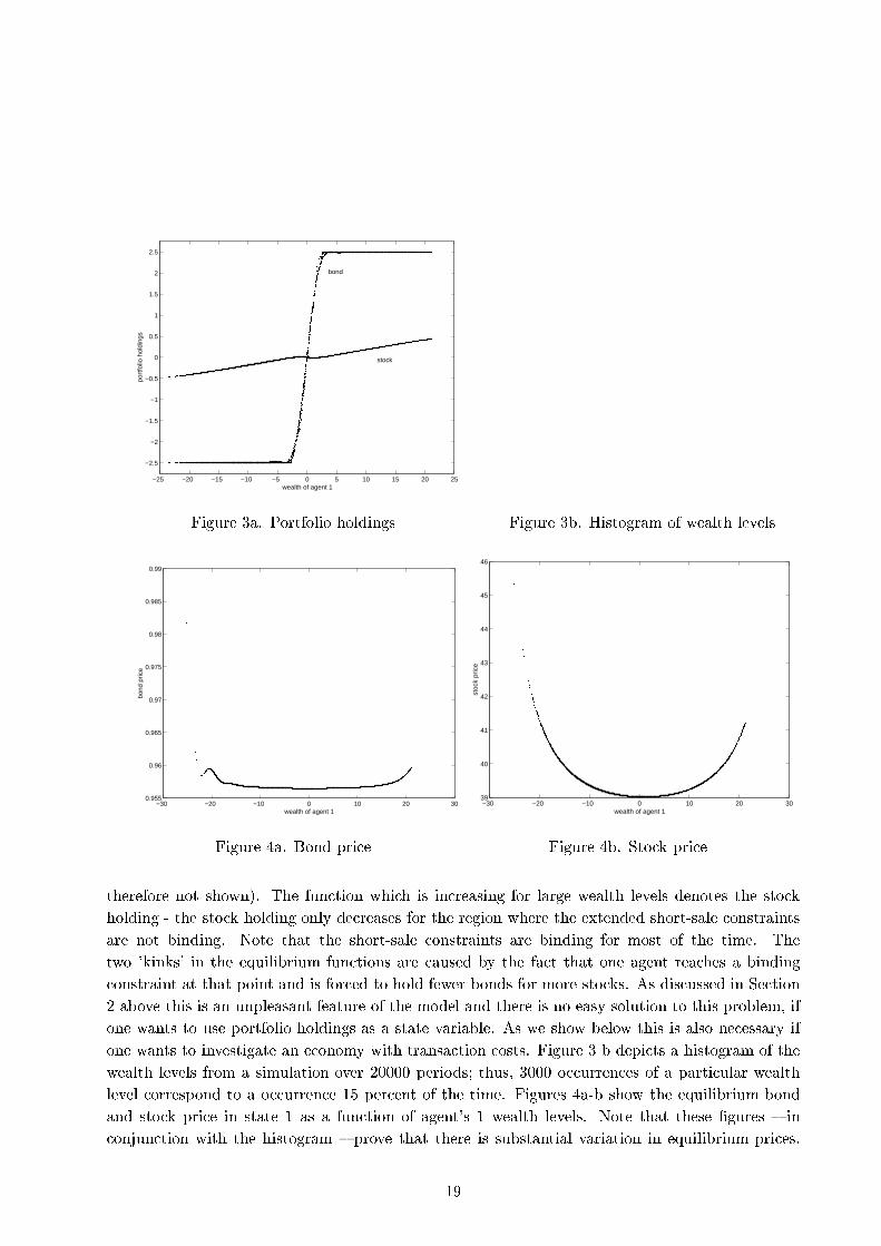
1CCCCCCCCCCCCCCA :The persisten e of the in ome distribution pro ess is omparable to the pro ess in Heaton andLu as (1996) (of ourse, Heaton and Lu as onsider a growing e onomy while we limit ourselves toan e onomy whi h is stationary in endowments).To �x ideas we start with the ase where there are no transa tion osts (i.e. � s = � b = 0) andwhere the short sale onstraints are given by �b1 = �2:5, �s1 = 0 , �b2 = 2:5 and �s2 = 0. That iswe do not allow short sales of the sto k but agents are allowed to borrow a substantial fra tion oftheir yearly in ome when poor.Identi al Preferen esWe �rst assume that both agents have identi al relative risk aversion of = 1:5. As explainedin Se tion 3 above we al ulate the equilibrium poli y fun tions as fun tions of portfolio holdings.Figure 1 shows the pri ing fun tion for the sto k pri e for state 1. In order to obtain a symmetri s ale we always refer to agent 1's net (a tual portfolio minus initial portfolio) asset holdings as16

Figure 1. Equilibrium pri ing fun tionequilibrium portfolios. The �gure tells us for every possible portfolio of agent 1 in period t� 1 thesto k pri e in period t; but it does not tell us whi h of these pri es a tually o ur on the equilibriumpath.Figure 1 is not very informative, be ause one needs to know whi h portfolio holdings o uralong a given equilibrium path. In order to investigate the equilibrium behavior of the model wesimulate the e onomy for 20000 periods (We a tually simulate for 21000 periods and only use thelast 20000 periods in order to eliminate any e�e ts whi h might be aused by initial onditions.).Figure 2 shows a s atter plot of all portfolio holdings whi h o ur along the equilibrium path.The result is very surprising: There is only a one-dimensional subset of equilibrium portfolioholdings; we refer to this set as the 'invariant' set. Note that the 8 diagonal lines in the Figure an be asso iated with the 8 di�erent states. Figure 2 suggests that for models without tradingfri tions there exists a one-to-one equilibrium relationship between the wealth of an agent and hisportfolio holdings.Note that although we hose the short-sale onstraints on the bond to be very weak theyare binding for most of the time. When they are not binding equilibrium sto k holdings arevery small and they only in rease as they hit the short-sale onstraint. In order to investigatethe relationship between wealth and portfolio holdings we plot the resulting equilibrium wealthlevels against portfolio holdings and pri es for ea h state. For the purposes of this se tion we17

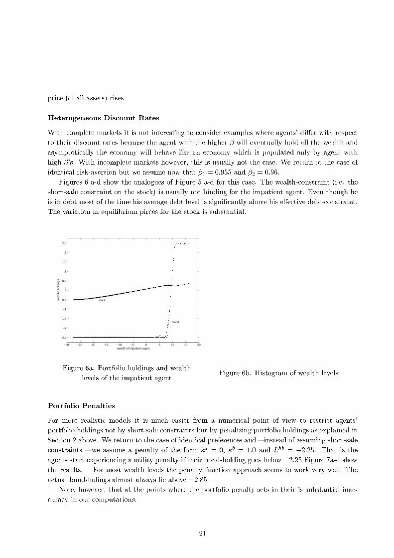
Figure 2. S atter plot of equilibrium portfoliosde�ne wealth as agent 1's wealth net of initial asset holdings i.e. wealth in period t is de�ned ase1(yt) + �1bt�1 + (�1st�1 � �1s�1)(qst + d(yt)). This has the advantage that the e onomy's total wealthalways sums up to aggregate endowments and is therefore independent of the wealth distribution(the wealth distribution for a model with H agents is thus (H � 1)-dimensional).It turns out that without fri tions the wealth level is in a one-to-one equilibrium relationshipwith the portfolio holdings (Kubler and S hmedders (2001) provide a theoreti al foundation forusing the agents' wealth distribution as the only endogenous state variable for stationary equilibriaand develop an algorithm for omputing su h equilibria.). In all subsequent �gures we will plot the omputed poli y fun tions against agent 1's wealth level sin e it provides a good way to illustrateour results. Note that we plot a tual simulated values along the equilibrium path. The only reasonthis is possible is that our results are very a urate so that even after 21000 periods the simulatedequilibrium portfolio holdings still almost lie in the one-dimensional invariant set. Using wealthas the state variable has the huge advantage that it allows us to plot the equilibrium values as afun tion of a single variable. While it an be rather hard to interpret three-dimensional surfa eplots of the equilibrium fun tions a two-dimensional graph is easy to interpret. We will thereforereport all transition fun tions as fun tions from wealth, although we have a tually omputed themas fun tions from portfolio holdings. Figure 3 a shows the equilibrium portfolio holdings in state1 asso iated with di�erent wealth levels (the �gures for the other states look very similar and are18

−25 −20 −15 −10 −5 0 5 10 15 20 25

−2.5

−2

−1.5

−1

−0.5

0

0.5

1

1.5

2

2.5

wealth of agent 1

port

folio

hol

ding

s

stock

bond

Figure 3a. Portfolio holdings Figure 3b. Histogram of wealth levels

−30 −20 −10 0 10 20 300.955

0.96

0.965

0.97

0.975

0.98

0.985

0.99

wealth of agent 1

bond

pric

e

Figure 4a. Bond pri e −30 −20 −10 0 10 20 3039

40

41

42

43

44

45

46

wealth of agent 1

stoc

k pr

ice

Figure 4b. Sto k pri etherefore not shown). The fun tion whi h is in reasing for large wealth levels denotes the sto kholding - the sto k holding only de reases for the region where the extended short-sale onstraintsare not binding. Note that the short-sale onstraints are binding for most of the time. Thetwo 'kinks' in the equilibrium fun tions are aused by the fa t that one agent rea hes a binding onstraint at that point and is for ed to hold fewer bonds for more sto ks. As dis ussed in Se tion2 above this is an unpleasant feature of the model and there is no easy solution to this problem, ifone wants to use portfolio holdings as a state variable. As we show below this is also ne essary ifone wants to investigate an e onomy with transa tion osts. Figure 3 b depi ts a histogram of thewealth levels from a simulation over 20000 periods; thus, 3000 o urren es of a parti ular wealthlevel orrespond to a o urren e 15 per ent of the time. Figures 4a-b show the equilibrium bondand sto k pri e in state 1 as a fun tion of agent's 1 wealth levels. Note that these �gures { in onjun tion with the histogram { prove that there is substantial variation in equilibrium pri es.19

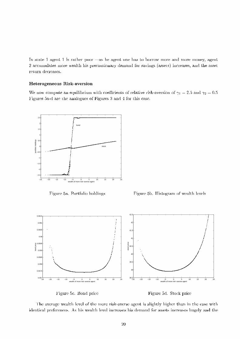
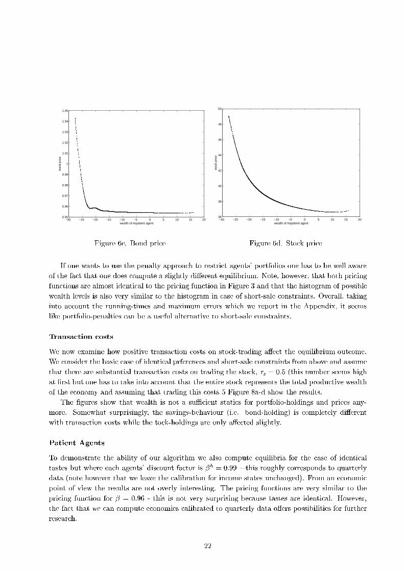
In state 1 agent 1 is rather poor { as he agent one has to borrow more and more money, agent2 a umulates more wealth his pre autionary demand for savings (assets) in reases, and the assetreturn de reases.Heterogeneous Risk-aversionWe now ompute an equilibrium with oeÆ ients of relative risk-aversion of 1 = 2:5 and 2 = 0:5Figures 5a-d are the analogues of Figures 3 and 4 for this ase.

−25 −20 −15 −10 −5 0 5 10 15 20 25

−2.5

−2

−1.5

−1

−0.5

0

0.5

1

1.5

2

2.5

port

folio

hol

ding

s

wealth of more risk−averse agent

bond

stock

Figure 5a. Portfolio holdings Figure 5b. Histogram of wealth levels

−25 −20 −15 −10 −5 0 5 10 15 20 250.957

0.9575

0.958

0.9585

0.959

0.9595

0.96

0.9605

0.961

0.9615

wealth of more risk−averse agent

bond

pric

e

Figure 5 . Bond pri e −25 −20 −15 −10 −5 0 5 10 15 20 2538.5

39

39.5

40

40.5

41

41.5

42

42.5

wealth of more risk−averse agent

stoc

k pr

ice

Figure 5d. Sto k pri eThe average wealth level of the more risk-averse agent is slightly higher than in the ase withidenti al preferen es. As his wealth level in reases his demand for assets in reases hugely and the20

pri e (of all assets) rises.Heterogeneous Dis ount RatesWith omplete markets it is not interesting to onsider examples where agents' di�er with respe tto their dis ount rates be ause the agent with the higher � will eventually hold all the wealth andasymptoti ally the e onomy will behave like an e onomy whi h is populated only by agent withhigh �'s. With in omplete markets however, this is usually not the ase. We return to the ase ofidenti al risk-aversion but we assume now that �1 = 0:955 and �2 = 0:96.Figures 6 a-d show the analogues of Figure 5 a-d for this ase. The wealth- onstraint (i.e. theshort-sale onstraint on the sto k) is usually not binding for the impatient agent. Even though heis in debt most of the time his average debt level is signi� antly above his e�e tive debt- onstraint.The variation in equilibrium pir es for the sto k is substantial.

−30 −25 −20 −15 −10 −5 0 5 10 15 20

−2.5

−2

−1.5

−1

−0.5

0

0.5

1

1.5

2

2.5

wealth of impatient agent

port

folio

hol

ding

s

stock

bond

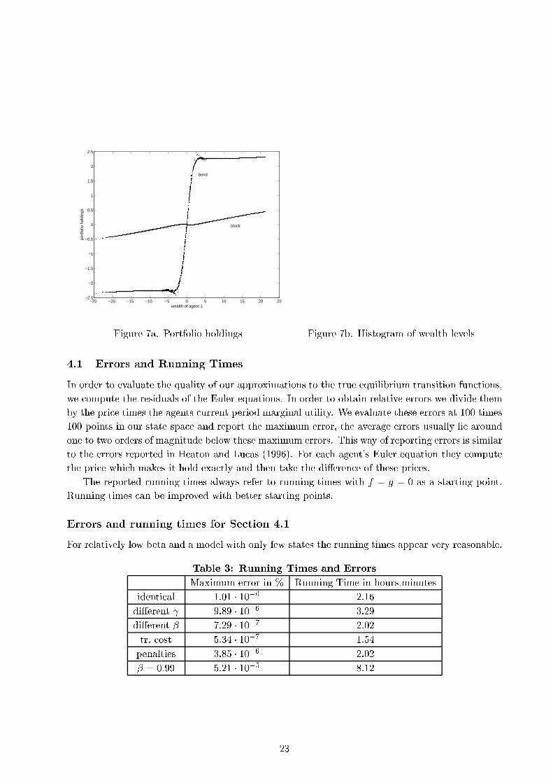
Figure 6a. Portfolio holdings and wealthlevels of the impatient agent Figure 6b. Histogram of wealth levelsPortfolio PenaltiesFor more realisti models it is mu h easier from a numeri al point of view to restri t agents'portfolio holdings not by short-sale onstraints but by penalizing portfolio holdings as explained inSe tion 2 above. We return to the ase of identi al preferen es and { instead of assuming short-sale onstraints { we assume a penalty of the form �s = 0, �b = 1:0 and Lhb = �2:25. That is theagents start experien ing a utility penalty if their bond-holding goes below �2:25 Figure 7a-d showthe results. For most wealth levels the penalty fun tion approa h seems to work very well. Thea tual bond-holings almost always lie above �2:85.Note, however, that at the points where the portfolio penalty sets in their is substantial ina - ura y in our omputations. 21

−30 −25 −20 −15 −10 −5 0 5 10 15 200.95

0.96

0.97

0.98

0.99

1

1.01

1.02

1.03

1.04

1.05

wealth of impatient agent

bond

pric

e

Figure 6 . Bond pri e −30 −25 −20 −15 −10 −5 0 5 10 15 2036

38

40

42

44

46

48

50

wealth of impatient agent

stoc

k pr

ice

Figure 6d. Sto k pri eIf one wants to use the penalty approa h to restri t agents' portfolios one has to be well awareof the fa t that one does ompute a slightly di�erent equilibrium. Note, however, that both pri ingfun tions are almost identi al to the pri ing fun tion in Figure 3 and that the histogram of possiblewealth levels is also very similar to the histogram in ase of short-sale onstraints. Overall, takinginto a ount the running-times and maximum errors whi h we report in the Appendix, it seemslike portfolio-penalties an be a useful alternative to short-sale onstraints.Transa tion ostsWe now examine how positive transa tion osts on sto k-trading a�e t the equilibrium out ome.We onsider the basi ase of identi al prferen es and short-sale onstraints from above and assumethat there are substantial transa tion osts on trading the sto k, �s = 0:5 (this number seems highat �rst but one has to take into a ount that the entire sto k represents the total produ tive wealthof the e onomy and assuming that trading this osts 5 Figure 8a-d show the results.The �gures show that wealth is not a suÆ ient stati s for portfolio-holdings and pri es any-more. Somewhat surprisingly, the savings-behaviour (i.e. bond-holding) is ompletely di�erentwith transa tion osts while the to k-holdings are only a�e ted slightly.Patient AgentsTo demonstrate the ability of our algorithm we also ompute equilibria for the ase of identi altastes but where ea h agents' dis ount fa tor is �h = 0:99 { this roughly orresponds to quarterlydata (note however that we leave the alibration for in ome states un hanged). From an e onomi point of view the results are not overly interesting. The pri ing fun tions are very similar to thepri ing fun tion for � = 0:96 - this is not very surprising be ause tastes are identi al. However,the fa t that we an ompute e onomies alibrated to quarterly data o�ers possibilities for furtherresear h. 22

−25 −20 −15 −10 −5 0 5 10 15 20 25−2.5

−2

−1.5

−1

−0.5

0

0.5

1

1.5

2

2.5

wealth of agent 1

port

folio

hol

ding

s

bond

stock

Figure 7a. Portfolio holdings Figure 7b. Histogram of wealth levels4.1 Errors and Running TimesIn order to evaluate the quality of our approximations to the true equilibrium transition fun tions,we ompute the residuals of the Euler equations. In order to obtain relative errors we divide themby the pri e times the agents urrent period marginal utility. We evaluate these errors at 100 times100 points in our state spa e and report the maximum error, the average errors usually lie aroundone to two orders of magnitude below these maximum errors. This way of reporting errors is similarto the errors reported in Heaton and Lu as (1996). For ea h agent's Euler equation they omputethe pri e whi h makes it hold exa tly and then take the di�eren e of these pri es.The reported running times always refer to running times with f = g = 0 as a starting point.Running times an be improved with better starting points.Errors and running times for Se tion 4.1For relatively low beta and a model with only few states the running times appear very reasonable.Table 3: Running Times and ErrorsMaximum error in % Running Time in hours.minutesidenti al 1:01 � 10�6 2.16di�erent 9:89 � 10�6 3.29di�erent � 7:29 � 10�7 2.02tr. ost 5:34 � 10�7 1.54penalties 3:85 � 10�6 2.02� = 0:99 5:21 � 10�5 8.1223

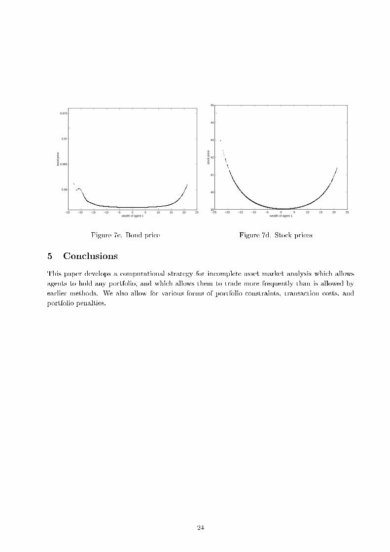
−25 −20 −15 −10 −5 0 5 10 15 20 25

0.96

0.965

0.97

0.975

wealth of agent 1

bond

pric

e

Figure 7 . Bond pri e −25 −20 −15 −10 −5 0 5 10 15 20 2539

40

41

42

43

44

45

wealth of agent 1

stoc

k pr

ice

Figure 7d. Sto k pri es5 Con lusionsThis paper develops a omputational strategy for in omplete asset market analysis whi h allowsagents to hold any portfolio, and whi h allows them to trade more frequently than is allowed byearlier methods. We also allow for various forms of portfolio onstraints, transa tion osts, andportfolio penalties.

24

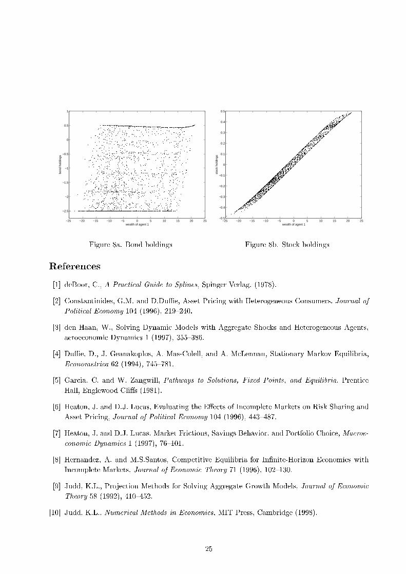
−25 −20 −15 −10 −5 0 5 10 15 20 25

−2.5

−2

−1.5

−1

−0.5

0

0.5

1

wealth of agent 1

bond

hol

ding

s

Figure 8a. Bond holdings −25 −20 −15 −10 −5 0 5 10 15 20 25−0.5

−0.4

−0.3

−0.2

−0.1

0

0.1

0.2

0.3

0.4

0.5

wealth of agent 1

stoc

k ho

ldin

gs

Figure 8b. Sto k holdingsReferen es[1℄ deBoor, C., A Pra ti al Guide to Splines, Spinger Verlag, (1978).[2℄ Constantinides, G.M. and D.DuÆe, Asset Pri ing with Heterogeneous Consumers, Journal ofPoliti al E onomy 104 (1996), 219{240.[3℄ den Haan, W., Solving Dynami Models with Aggregate Sho ks and Heterogeneous Agents,a roe onomi Dynami s 1 (1997), 355{386.[4℄ DuÆe, D., J. Geanakoplos, A. Mas-Colell, and A. M Lennan, Stationary Markov Equilibria,E onometri a 62 (1994), 745{781.[5℄ Gar ia, C. and W. Zangwill, Pathways to Solutions, Fixed Points, and Equilibria, Prenti eHall, Englewood Cli�s (1981).[6℄ Heaton, J. and D.J. Lu as, Evaluating the E�e ts of In omplete Markets on Risk Sharing andAsset Pri ing, Journal of Politi al E onomy 104 (1996), 443{487.[7℄ Heaton, J. and D.J. Lu as, Market Fri tions, Savings Behavior, and Portfolio Choi e, Ma roe- onomi Dynami s 1 (1997), 76{101.[8℄ Hernandez, A. and M.S.Santos, Competitive Equilibria for In�nite-Horizon E onomies withIn omplete Markets, Journal of E onomi Theory 71 (1996), 102{130.[9℄ Judd, K.L., Proje tion Methods for Solving Aggregate Growth Models, Journal of E onomi Theory 58 (1992), 410{452.[10℄ Judd, K.L., Numeri al Methods in E onomi s, MIT Press, Cambridge (1998).25

−25 −20 −15 −10 −5 0 5 10 15 20 250.955

0.96

0.965

0.97

0.975

0.98

0.985

0.99

0.995

wealth of agent 1

bond

pric

e

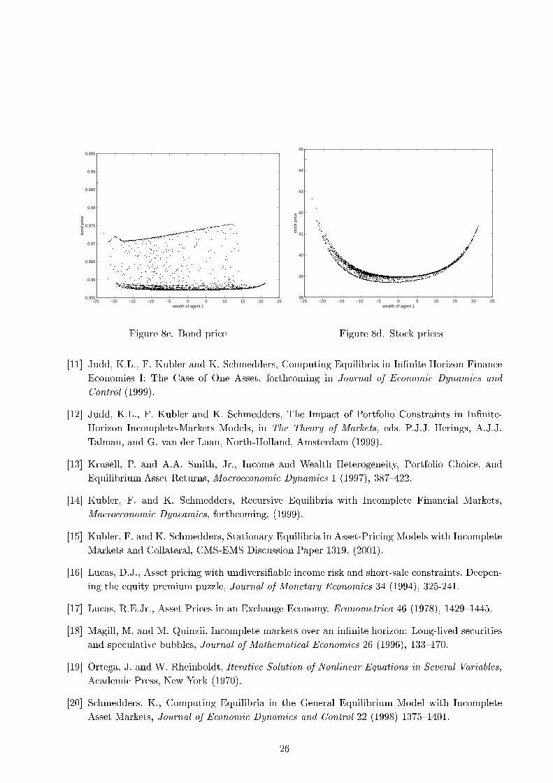
Figure 8 . Bond pri e −25 −20 −15 −10 −5 0 5 10 15 20 2538

39

40

41

42

43

44

45

wealth of agent 1

stoc

k pr

ice

Figure 8d. Sto k pri es[11℄ Judd, K.L., F. Kubler and K. S hmedders, Computing Equilibria in In�nite Horizon Finan eE onomies I: The Case of One Asset, forth oming in Journal of E onomi Dynami s andControl (1999).[12℄ Judd, K.L., F. Kubler and K. S hmedders, The Impa t of Portfolio Constraints in In�nite-Horizon In omplete-Markets Models, in The Theory of Markets, eds. P.J.J. Herings, A.J.J.Talman, and G. van der Laan, North-Holland, Amsterdam (1999).[13℄ Krusell, P. and A.A. Smith, Jr., In ome and Wealth Heterogeneity, Portfolio Choi e, andEquilibrium Asset Returns, Ma roe onomi Dynami s 1 (1997), 387{422.[14℄ Kubler, F. and K. S hmedders, Re ursive Equilibria with In omplete Finan ial Markets,Ma roe onomi Dyn ami s, forth oming, (1999).[15℄ Kubler, F. and K. S hmedders, Stationary Equilibria in Asset-Pri ing Models with In ompleteMarkets and Collateral, CMS-EMS Dis ussion Paper 1319, (2001).[16℄ Lu as, D.J., Asset pri ing with undiversi�able in ome risk and short-sale onstraints. Deepen-ing the equity premium puzzle, Journal of Monetary E onomi s 34 (1994), 325-241.[17℄ Lu as, R.E.Jr., Asset Pri es in an Ex hange E onomy, E onometri a 46 (1978), 1429{1445.[18℄ Magill, M. and M. Quinzii, In omplete markets over an in�nite horizon: Long-lived se uritiesand spe ulative bubbles, Journal of Mathemati al E onomi s 26 (1996), 133{170.[19℄ Ortega, J. and W. Rheinboldt, Iterative Solution of Nonlinear Equations in Several Variables,A ademi Press, New York (1970).[20℄ S hmedders, K., Computing Equilibria in the General Equilibrium Model with In ompleteAsset Markets, Journal of E onomi Dynami s and Control 22 (1998) 1375{1401.26

[21℄ Telmer, C.I. Asset-Pri ing Puzzles in In omplete Markets. Journal of Finan e 48 (1993), 1803{1832.[22℄ Watson, L.T., S.C. Billups, and A.P. Morgan, HOMPACK: A Suite of Codes for GloballyConvergent Homotopy Algorithm, ACM Transa tions on Mathemati al Software 13 (1987),281{310.[23℄ Zeidler, E., Nonlinear Fun tional Analysis and Its Appli ations I, Springer Verlag, New York(1986).[24℄ Zhang, H.H., Endogenous Borrowing Constraint with In omplete Markets, Journal of Finan e(1997a), 2187{2209.[25℄ Zhang, H.H., Endogenous Short-Sale Constraint, Sto k Pri es and Output Cy les, Ma roe o-nomi Dynami s 1 (1997b), 228{254.

27