Embed Size (px)
Citation preview
ILL I N 0 I SUNIVERSITY OF ILLINOIS AT URBANA-CHAMPAIGN
PRODUCTION NOTE
University of Illinois atUrbana-Champaign Library
Large-scale Digitization Project, 2007.

UNIVERSITY OF ILLINOIS BULLETINIsSSD TWICE A WEEK
Vol. XXXV November 30, 1937 No. 27
[Entered' as second-class matter December 11, 1912, at the- post office at Urlana, Illinois, underthe Act of August 24, 1912. Acceptance for mailing at the special rate of postage provided
for in section 1103. Act of October 3, 1917, authorized July 31, 1918.]
SOLUTION OF ELECTRICAL NETWORKSBY SUCCESSIVE APPROXIMATIONS
BYLARENCE L. SMITH
LAURENCE L. SMITH
BULLETIN No. 299
ENGINEERING EXPERIMENT STATIONPssmn pr Tws UNvZRaST OF ILLmNOIs. UBAiA
?AoPE: Fowrr-nvt CTk
T HE Engineering Experiment Station was established by actof the Board of Trustees of the University of Illinois on De-
cember 8, 1903. It is the purpose of the Station to conduct
investigations and make studies of importance to the engineering,
manufacturing, railway, mining, and other industrial interests of the
State.The management of the Engineering Experiment Station is vested
in an Executive Staff composed of the Director and his Assistant, theHeads of the several Departments in the College of Engineering, andthe Professor of Industrial Chemistry. This Staff is responsible forthe establishment of general policies governing the work of the Station,including the approval of material for publication. All members ofthe teaching staff of the College are encouraged to engage in scientificresearch, either directly or in co6peration with the Research Corps,composed of full-time research assistants, research graduate assistants,and special investigators.
To render the results of its scientific investigations available tothe public, the Engineering Experiment Station publishes and dis-tributes a series of bulletins. Occasionally it publishes circulars oftimely interest, presenting information of importance, compiled fromvarious sources which may not readily be accessible to the clienteleof the Station, and reprints of articles appearing in the technical presswritten by members of the staff.
The volume and number at the top of the front cover page aremerely arbitrary numbers and refer to the general publications of theUniversity. .ither above the title or below the seal is given the num-ber of the Engineering Experiment Station bulletin, circular, or reprintwhich should be used in referring to these publicatiohs.
IFor copies of publications or for other information addressTHE ENGINEERING EXPERIMENT STATION,
IfNIVASITYr oF IlNOIS,
URBANA, ILLINOIS
* I, * : ' - ' -^ '*' , " 1
; .. ;1
" :' 1
^ ' '* *. .

UNIVERSITY OF ILLINOISENGINEERING EXPERIMENT STATION
BULLETIN No. 299 NOVEMBER, 1937
SOLUTION OF ELECTRICAL NETWORKSBY SUCCESSIVE APPROXIMATIONS
BY
LAURENCE L. SMITHASSOCIATE IN ELECTRICAL ENGINEERING
ENGINEERING EXPERIMENT STATIONPUBLISHED BY THE UNIVERSITY OF ILLINOIS, URBANA

3000-12-37-13321 PRESS ,
CONTENTS
I. INTRODUCTION . . . . .
1. Introductory . . . . . . . . . . .2. Acknowledgments . . . . . .
II. DISCUSSION OF METHODS OF SOLUTION . . . . .
3. Methods Available . . . . . . . . .4. Solution by Calculating Tables . . . . .5. Solution by Simultaneous Equations . . . .6. Solution by Trial and Error . . . . .7. Solution by Simplification of Network .8. Solution by Method of Successive Approximations
III. METHOD OF BALANCING VOLTAGE DROPS . . . .
9. Description . . . . . . . . . . .10. Illustrative Problem-Single d-c. Loop .11. Illustrative Problem-Two-Loop d-c. Circuit
IV. METHOD OF BALANCING CURRENTS . . . . .
12. Description . . . . . . . . . .13. General Proof . . . . . . . . .14. Illustrative Problem-Single d-c. Loop15. Illustrative Problem-Two-Loop d-c. Circuit16. Illustrative Problem-Three-Loop d-c. Circuit17. Illustrative Problem-Modification of Method
Used in Section 16 . . . . . . .18. Illustrative Problem-Partial Excess Method
V. SOLUTION OF TYPICAL NETWORK PROBLEM
19. Statement of Problem . . . . .20. Solution by Simultaneous Equations .21. Solution by Balancing Voltage Drops22. Solution by Balancing Currents
VI. CONCLUSIONS . . . . . . . . .
23. Method of Balancing Voltage Drops24. Method of Balancing Currents
APPENDIX A . . . . . . . . . . .Suggested Forms . . . . .
APPENDIX B . . . . . . . . . . .Bibliography . . . . . . . .
. . . . 27
. . . . 27
. . . . 28
. . . . 29
. . . . 29
. . . . 33
. . . . 33
. . . . 33
. . . . 35
. . . . 35
. . . . 38
. . . . 38
PAGE
555
5566788
10101012
141414202021
2425
LIST OF FIGURES
NO. PAGE
1. Envelope Curve for Approximations-Load Current . . . . . . . 31
2. Envelope Curve for Approximations-Input Current . . . . . . . 31
3. Envelope Curve for Approximations-Network Current . . . . . . 32
SOLUTION OF ELECTRICAL NETWORKS BYSUCCESSIVE APPROXIMATIONS
I. INTRODUCTION
1. Introductory.-The calculation of voltage and current condi-tions in electrical networks becomes increasingly important as centralstation systems grow and their proper operation becomes more im-portant to insure continuity of service to each load carried. Voltageregulation, current division between paths, transmission efficiencies,and selective operation of relays must be known for the present sys-tem or for the system resulting after proposed additions to the presentsystem, either under normal operation or under short circuit condi-tions. Unfortunately, as the importance of calculating such con-ditions increases, so also does the difficulty of making such calculationsincrease.
It is the purpose of this bulletin to present an additional methodof solving these networks. Other methods are available, but it is feltthat this method has considerable merit, particularly when applied tothe solution of a-c. secondary networks or the usual transmission linesystems. Although the method, as presented in this paper, is appliedto a-c. and d-c. power networks, it should be borne in mind that themethod is applicable to any network composed of invariable pa-rameters which are constant with respect to time. The discussion ofthe advantages and limitations of this method will be confined to acomparison with other existing methods used in d-c. or a-c. powernetwork problems.
2. Acknowledgments.-The writer wishes to express his apprecia-tion for the assistance and suggestions given by PROF. HARDY CROSSand MR. L. B. ARCHER in the preparation of this manuscript.
II. DIscussioN OF METHODS OF SOLUTION
3. Methods Available.-Various methods of attack in obtainingthe solution of electrical networks have been devised and are in use.These methods may be grouped into five general classifications:
(a) Solution by calculating tables
(b) Solution by simultaneous equations(c) Solution by trial and error
(d) Solution by simplification of the network
(e) Solution by method of successive approximations
5
ILLINOIS ENGINEERING EXPERIMENT STATION
4. Solution by Calculating Tables.-Calculating tables* were orig-inally devised by H. H. Dewey and W. W. Lewis. These tables weregroups of variable calibrated resistances with plug-in leads by whichany electrical network could be duplicated by a proper set-up ofresistances on the table. A d-c. voltage was applied at the generatingsource, and the resultant currents read in each branch of the network.The value of the resistance inserted in each branch was determined bythe value of the reactance in that particular branch of the actualnetwork being studied. The resistance of the actual network wasneglected. These tables were mainly used in finding short-circuitconditions. Their use in studying normal operating conditions wasslight, since phase displacements of generated voltages and impedanceangles of the network could not be duplicated by such a d-c. table.
A-c. calculating tablest are an extension of the principles used inthe d-c. calculating tables, in that the actual system is duplicated inthe laboratory by means of the calculating table. It consists of manyvariable resistors, inductances, and capacitances, so that each unit ofthe actual network may be accurately duplicated, and these unitscombined into a network such as the one to be studied. An a-c.voltage is applied, and the currents in each branch are measured.Phase shifters may be used to simulate the phase displacements involtages of the alternators on the actual system.
Short-circuit conditions or normal operating conditions may bestudied on this type of set-up, since the actual system is very exactlyduplicated. Its accuracy is mainly limited by the evaluation of theconstants in the actual system.
The chief disadvantage of the calculating table method is its cost.Few companies, though much interested in network problems, couldjustify the purchase of such a table. As a result, few tables are nowavailable, and many problems worthy of solution are not solved bythis method.
5. Solution by Simultaneous Equations.-The solution of a net-work by simultaneous equations is so generally known that littlereference to the method need be made. The simultaneous equationsare set up to satisfy the two fundamental laws of electrical circuits,known as Kirchhoff's Laws. The first law states that the total cur-
*G. E. Rev., p. 901, 1916.G. E. Rev., Vol. 22, p. 140, 1919.G. E. Rev., p. 669, 1920.Elec. World, p. 985, 1922.Elec. World, p. 707, 1923.
tTrans. A. I. E. E., p. 10, 1923.G. E. Rev., p. 611, 1923.Trans. A. I. E. E., p. 831, 1923.Trans. A. I. E. E., p. 72, 1925.

SOLUTION OF ELECTRICAL NETWORKS
rent flowing into each junction is zero. The second law states thatthe total drop in voltage around each closed loop is zero. To deter-mine the voltage drop in a particular branch, Ohm's Law as appliedto alternating current is used. This law states that the voltage dropacross an impedance is equal to the product of the current flowthrough it and the value of the impedance. The set of simultaneousequations, so obtained, may be solved to obtain the current flowingin each branch. If the number of equations is large, this process isan extremely tedious and cumbersome one. The process may beshortened by the use of determinants, but the calculations are diffi-cult to check, and the intermediate steps in the solution do not havea physical significance that is easy to grasp.
6. Solution by Trial and Error.-The solution of networks by thetrial-and-error method, as described in the brief literature available,seems to be a rather unorganized method of procedure which dependsto a large extent upon the judicious use of quite complete engineeringexperience possessed by the person using the method.
One such method is outlined by H. H. Spencer and H. L. Hazen.*Quoting: "By this method, a voltage is assumed at the load mostremote from a generating station. Knowing the kv-a. and powerfactor drawn, the current is calculated, and the drop due to it, overthe line to the next load, added to the assumed voltage. This loadcurrent may then be found, the drop due to both currents in thenext section of line added to obtain the next junction voltage, andso on, until the generating station is reached. The discrepancy be-tween this voltage and that known to exist at the generating stationis used in making a new trial voltage assumption at the first load, andthe problem worked through again. This procedure is continueduntil a sufficiently close check is obtained for the work in hand."
It is all too evident that the method here suggested would be verydifficult to use unless the loads are on a single loop system. Branchcurrents in a network could not be guessed accurately enough, bythis method, to insure the same voltage rise from the load to thegenerating station, regardless of the path taken. Therefore the dif-ference between the calculated voltage and the known voltage at thegenerator would be, at best, a very questionable indication uponwhich to base the new assumed values. Problems to which thismethod might be applied will lend themselves readily to more rigorousanalytical methods.
*Trans. A. I. E. E., p. 72, 1925.

ILLINOIS ENGINEERING EXPERIMENT STATION
Woodruff* outlines a cut-and-try method which, upon examina-tion, reveals that much ingenuity and engineering knowledge is re-quired if this method is to be used with any degree of success. Itis mentioned by him, however, that the voltage drops caused by theassumed currents, when summed around any closed loop, may be usedas a guide in assuming more correct current values. No definitemethod of procedure is described. Quoting (p. 200) "Each networkpresents a new problem, and no definite rules can be given whichhold for all networks." Dahlt (p. 2) gives a short description similarto that just given.
7. Solution by Simplification of Network.-A solution accomplishedby simplification of the network is explained in detail in severalsources,$ only a few of which are listed. By means of transformationsthe network may be reduced to a single equivalent impedance be-tween two points. Usually it is necessary to simplify the networkby steps through a repeated application of transformations. Themost commonly used method is the delta-wye or wye-delta trans-formation.¶ Another method, less often used, is the star-mesh trans-formation.§ However, this method, in general, will not convert amesh into a star. In networks where load is tapped off at a pointother than a junction, Fortescue** shows a method which leaves thenetwork unaffected, where a portion of that load may be placed ateach of the junctions nearest it-leaving the line between thesejunctions untapped.
These methods have many useful applications, but it is necessaryto assume that all generated voltages in the system are exactly equal,and in phase, before the system may be reduced to a single equivalentimpedance. If the current in a particular branch of the network isdesired, it is necessary to reverse the process and reconstruct thenetwork before that current may be found. The method is reversible,but the work involved in this double process is sometimes almostprohibitive. It may, however, be found advisable to utilize some ofthese methods in a partial simplification of the network, before othermethods of solution are utilized.
8. Solution by Method of Successive Approximations.-Althoughthe method of successive approximations might be considered a cut-
*Woodruff, L. F., "Principles of Electric Power Transmission and Distribution," Chap. XIV,John Wiley and Sons Inc., New York, 1925.
tDahl, 0. B. C., "Electric Circuits Theory and Applications," Chap. I, Vol. I, McGraw-HillBook Co., 1928.
tElec. Jour., p. 344, 1019.¶Elec. World and Eng., Vol. XXXIV, p. 413, 1899.iJour. I. E. E. (London), Vol. 62, p. 916.
*NElec. Jour., p. 344, 1919.
SOLUTION OF ELECTRICAL NETWORKS
and-try method, it is sufficiently different to warrant a separateclassification. The methods discussed under this heading differ fromthe strict cut-and-try method in that, after the first assumption ofvalues, the method leads very definitely and surely to the correct solu-tion, without further exercise of judgment in making new assumptions.
The method of superposed solutions assumes power factors andvoltages at the various load points. Then the principle of unit cur-rent is employed. By this method the current distribution in thenetwork, for a single load, is found. Finding this distribution foreach load, the actual resultant currents in the network are found bysuperposing each of these solutions upon the other. Fortescue*describes the method in these terms (p. 350): "If a number of currentsare drawn from a network at various points, the resulting distributionof currents in the invariable portions of the network will be the sameas that obtained by considering each load separately and superposingthe separate solutions; the currents in the various portions of thenetwork being combined vectorially."
The amount of work involved in this method of solution is notsmall, since each separate solution is a network problem in itself. Itsmain advantage lies in the fact that the addition of a load to a presentsystem merely requires the separate solution for that load only, andthis solution may be superposed upon the solution of the presentsystem. However, if a new path is added to the network, all formersolutions must be recalculated. Also, if the original assumptions ofvoltages and power factors were incorrect, a new, or several newsolutions will be required. This difficulty assumes sizable propor-tions when it is realized that the individual load currents must bechosen at the proper phase relationship with respect to one particularvoltage vector, common to all. It is not sufficient to assume thesepower factors with respect to their respective load voltages which areshifted in phase with respect to each other, because of the networkimpedance drops.
The method to be described in this paper is based upon the workdone by Hardy Crosst in the solution of water flow through intercon-nected systems of pipes. Quoting (p. 8) "Two methods of analysis areproposed. In one of these, the flows in the pipes or conductors of thenetwork always satisfy the condition that the total flow into and outof each junction is zero, and these flows are successively corrected tosatisfy the condition of zero total change of head around each circuit.In the other method, the total change of head around each circuit
*Elec. Jour., p. 344, 1919.fUniv. of Ill. Eng. Exp. Sta. Bul. 286, "Analysis of Flow in Networks of Conduits or Conductors,"
1936.
ILLINOIS ENGINEERING EXPERIMENT STATION
always equals zero, and the flows in the pipes of the circuit aresuccessively adjusted so that the total flow into and out of eachjunction finally approaches or becomes zero."
The following portions of the paper will describe each of thesemethods as applied to d-c. and a-c. networks. Illustrative examplesof such solutions will be given and the advantages, disadvantages,and limitations of the method discussed.
III. METHOD OF BALANCING VOLTAGE DROPS
9. Description.-The method of solution by successive approxima-tions is based upon the premise that all currents are assumed so asto satisfy the condition that the total flow into or out of each junctionis zero, and these assumed values are successively corrected to satisfythe condition of zero total drop of voltage around each closed loop.The amount by which the total voltage drop around a closed loop isgreater than, or less than, zero determines the amount by which theassumed current values should be increased or decreased. Thismethod is applied as often as is necessary to reach the degree ofaccuracy desired.
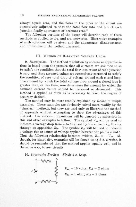
The method may be more readily explained by means of simpleexamples. These examples are obviously solved more readily by the"classical" methods, but they are used only to illustrate the methodof approach without attempting to show the advantages of thismethod. Currents and oppositions will be denoted by subscripts inthis and other examples to follow. The symbol Vab will be used toindicate a voltage drop from a to b caused by the current lab flowingthrough an opposition Zab. The symbol Eab will be used to indicatea voltage rise or source of voltage applied between the points a and b.Thus the following relationship becomes evident, Eab = - Vab. Al-though, for simplicity, examples will be shown using d-c. circuits, itshould be remembered that the method applies equally well, and inthe same way, to a-c. circuits.
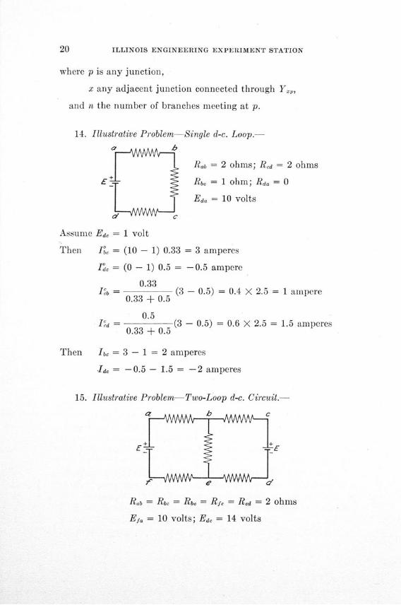
10. Illustrative Problem-Single d-c. Loop.-0a AAAAAAA
Ea. = 10 volts; Rab = 2 ohmsE
Rbc = 1 ohm; Red = 2 ohms
SOLUTION OF ELECTRICAL NETWORKS
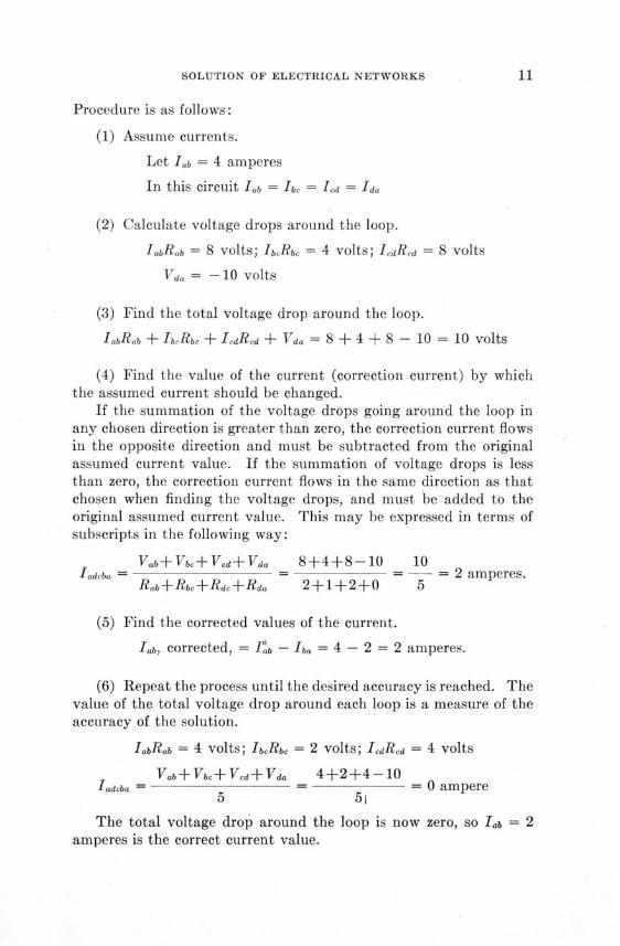
Procedure is as follows:
(1) Assume currents.
Let lab = 4 amperes
In this circuit lab = Ibc = Icd = Ida
(2) Calculate voltage drops around the loop.
IabRab = 8 volts; IbRbc = 4 volts; IcdRd = 8 volts
Vda = -10 volts
(3) Find the total voltage drop around the loop.
IabRab + IbcRbc + IcdRcd + Vda = 8 + 4 + 8 - 10 = 10 volts
(4) Find the value of the current (correction current) by whichthe assumed current should be changed.
If the summation of the voltage drops going around the loop inany chosen direction is greater than zero, the correction current flowsin the opposite direction and must be subtracted from the originalassumed current value. If the summation of voltage drops is lessthan zero, the correction current flows in the same direction as thatchosen when finding the voltage drops, and must be added to theoriginal assumed current value. This may be expressed in terms ofsubscripts in the following way:
Vab+Vbc±Vcd+Vda 8+4+8-10 10Iadcba ------ +----- 84 -- 10 2 amperes.
Rab+Rbc+Rde±Rda 2+1+2+0 5
(5) Find the corrected values of the current.
lab, corrected, = Iab - Iba = 4 - 2 = 2 amperes.
(6) Repeat the process until the desired accuracy is reached. Thevalue of the total voltage drop around each loop is a measure of theaccuracy of the solution.
IabRab = 4 VOlts; IbcRbc = 2 volts; IcdRed = 4 volts
Vab+Vbc+Vcd+Vda 4+2+4-10Iadcba = - = 0 ampere
5 51
The total voltage drop around the loop is now zero, so lab = 2amperes is the correct current value.
ILLINOIS ENGINEERING EXPERIMENT STATION
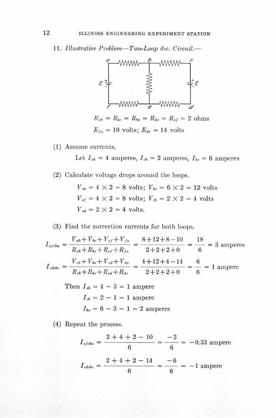
11. Illustrative Problem-Two-Loop d-c. Circuit.-
Ir E
Rab = Rbe = Rbe = Rde = Ref = 2 ohms
Efa = 10 volts; Ed, = 14 volts
(1) Assume currents.
Let lab = 4 amperes, Icb = 2 amperes, Ib, = 6 amperes
(2) Calculate voltage drops around the loops.
Vab = 4 X 2 = 8 volts; Vbe = 6 X 2 = 12 volts
Vf = 4 X 2 = 8 volts; Vb = 2 X 2 = 4 volts
V,d = 2 X 2 = 4 volts.
(3) Find the correction currents for both loops.
Vab+Vbe+Vef+Vfa 8+12+8-10 18Iafeba = - = 3 amperes
Rb++Rb++R,.+Rf. 2+2+2+0 6
Vd b+Vbe+Vea+Vdc 4+12+4-14 6Icdebc = ---- =-- = - = 1 ampere
Reb+Rb,+Red+Rde 2+2+2+0 6
Then I, = 4 - 3 = 1 ampere
Ib = 2 - 1 = 1 ampere
Ibe = 6 - 3 - 1 = 2 amperes
(4) Repeat the process.
2+4+2-10 -2Iafeba = - = -0.33 ampere
6 6
2+4+2-14 -6Icdebc ---- = - = - 1 ampere
6 6

SOLUTION OF ELECTRICAL NETWORKS
lab = 1 + 0.33 = 1.33 amperes
Icb = 1 + 1 = 2.00 amperes
Ibe = 2 + 1 + 0.33 = 3.33 amperes
2.67 + 6.66 + 2.67 - 10 2Iafeba = = - = 0.33 ampere
6 6
4 + 6.667 + 4 - 14 0.67Icdebc = - = 0.11 ampere
6 6
Iab = 1.33 - 0.33 = 1.00 ampere
Icb = 2 - 0.11 = 1.89 amperes
Ibe = 3.33 - 0.33 - 0.11 = 2.89 amperes
2 + 5.78 + 2 - 10 -0.22afeba = -- = -0.04 ampere
6 6
3.78 + 5.78 + 3.78 - 14 -1.34Icdebc = - = -0.22 ampere
6 6
Iab = 1.00 + 0.04 = 1.04 amperes
Ib = 1.89 + 0.22 = 2.11 amperes
Ib. = 2.89 + 0.04 + 0.22 = 3.15 amperes
The correct values are
Iab = 1 ampere; Ilb = 2.0 amperes; Ibe = 3.0 amperes
This problem might also be worked one loop at a time; first oneloop, and then the other.
Iab = 4 amperes; Icb = 2 amperes; Ibe = 6 amperes
8+ 12+8- 10 18lafeba = - = 3 amperes
6 6
Iab = 4 - 3 = 1 ampere; Icb = 2 amperes; Ibe = 6 - 3 = 3 amperes
4+6+4-14 0Icdebc = = - = 0 ampere
6 6
Iab = 1 ampere; Icb = 2 amperes; Ibe = 3 amperes

ILLINOIS ENGINEERING EXPERIMENT STATION
The assumed values of current in this case were such that thesecond loop was balanced by the first correction on the first loop.It must not be concluded that this second method arrives at thedesired result much more rapidly than the former method. It doescorrect itself more rapidly, but this obvious advantage may be out-weighed by the fact that, for the more involved circuits, each currentwill require several corrections during the process of considering eachloop of the network once. Either of the two methods may be used.The choice of methods will depend upon the operator's ability andindividual experience with each. The method, as illustrated, neednot be rigorously followed. The correction current may be given anyvalue desired, which in the engineering judgment of the user willcause the voltage drops in each loop to become zero after fewercorrections. The sum of the voltage drops in each closed loop maybe used merely as a guide in determining the direction of, and theamount of, correction current to use. Such engineering judgment willshorten the method both by its use during the calculations, and inthe choice of original assumed values of the currents. As the userbecomes acquainted with the method such choice will be more easilymade. However, in any case, if the method is rigorously followed,the correct solution will surely result. It should be pointed out thatthe original assumed values of the currents used in these illustrativeproblems were purposely chosen at unlikely figures so as to betterillustrate the method.
IV. METHOD OF BALANCING CURRENTS
12. Description.-This method employs the fact that the voltagedrops around each closed loop must equal zero. The potential ateach junction is assumed, and the current in each branch caused bythe resultant potential differences is found. The sum of these cur-rents at each junction is found, and, if this is not zero, the currents arecorrected successively until their sum at each junction approaches zerowithin the desired degree of accuracy. This is done in such a mannerthat the total voltage drop around each closed loop remains equal tozero. The excess or deficit current* at each junction is distributedover the branches as shown in the following. Proof of the correctnessof the method is also given.
13. General Proof.-Consider the simple single junction circuitshown where the potentials at a, b, and d are known with respectto a reference point o.
*Hereafter a deficit will be treated as a negative excess; only excesses are considered to exist.
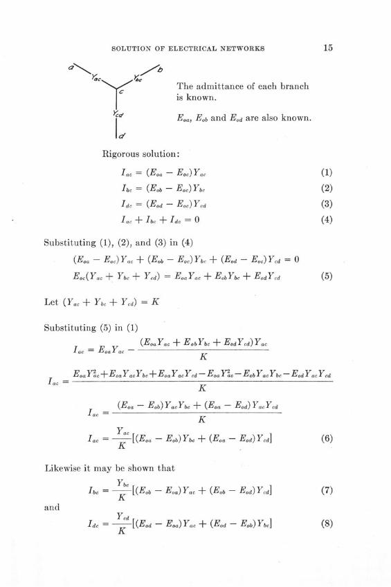
SOLUTION OF ELECTRICAL NETWORKS
The admittance of each branchis known.
Eoa, Eob and Eod are also known.
Rigorous solution:
lac = (Eoa - Eoo)Yac (1)
Ibc = (Eob - Eoc) Yb, (2)
Idc = (Eod E- Eoc) Yd (3)
la• + e + Ido = 0 (4)
Substituting (1), (2), and (3) in (4)
(Eoa - Eoc) Yao + (E 0 b - E.e) Ybc + (Eod - Eo) Yda = 0
Eo(Yac + Yb0 + Ycd) = EoaYa + Eob Yb + EoaYcd (5)
Let (Yac + Ybc + Yod) = K
Substituting (5) in (1)
(Eoa.Yac + EobYbc + EdaYcd) YacI o = EoYac -
K
Eoa Y + Eoa YacYbc + Eoa Yac Yd - Eoa Yc- Eob Yac Ybc- Eod Yac Ycd
K
(Eoa - Eob) YaoYb + (Eoa - Eod) YacYcdlac --
KYac
lac = -- [(Eoa - Eob) Yb + (Eoo - Eod) Yda] (6)K
Likewise it may be shown that
YbcIbo = --Y[(Eob - Eoa) Yac + (Eob - Eod) Ycd] (7)
Kand
VYIdc = -L[ (Eod - Eoa) Yao + (Eod - Eob) Ybj
K
ILLINOIS ENGINEERING EXPERIMENT STATION
Assuming a voltage at c equal to E°,
Iac = (Eoa - E.c) Yac (9)
Ibc = (E0 b - Eoc) Ybc (10)
I°dc = (Eod - E~oc)Ycd (11)
Let Ic be the correction current to be added to each of the currentsjust found to obtain the correct values lac, Ibc and Ied as calculatedby the previous rigorous solution.
Theniae = Tic + i c = - Ica
Use the second form for convenience; then
Ica = Iac - lac (12)
Ib = Iob - Ibe (13)
Id = Idc - Id, (14)
Substituting (9) and (6) in (12)
1Ia = (Eo, - Ec0) Yac - Y-- [(Eoa - Eob) Ybc + (Eo. - Eod) Ycd]K
YaclIa = (EoaYac + EoaYbc + EoaYcd - EoaYbc + Eob Yb - Eoa Yd +
KEodYcd - EgcK)
Yaca = --- (Eoayac + Eob Yb + EodYFd - EgcK)
K
Yac
Ia = - [(Eo. - ESo) Yac + (Eob - E'l) Ybc + (ESd - E.c) Yad]K
YacIa = K (I°ae + lio + Idc) (15)
Likewise it may be shown that
Ybcb = -- -(Ic + Ioe + I°d) (16)
Ied = -(KIo + I, + Idc) (17)A.

SOLUTION OF ELECTRICAL NETWORKS
Since K = Yac + Yb, + Ycd, it is evident that
la + Icb + I'd = IL, + IL + Idc
Therefore all the excess has been distributed so that the sum ofthe currents is zero after the corrections just derived have beenapplied.
This derivation was based on the assumption that the voltagesEoa, Eob and Evd were known. Then Eoc is corrected to its propervalue with respect to Eoa, Eob, and Eod by distributing the excessat c as in the foregoing. If E0o, Eob, and Eod are assumed values thatmust also be corrected by the method employed at junction c, anexcess will again arise at junction c and may be treated in the samefashion. This process is used at each junction, and the new excessesarising at each junction are then handled as were the original excesses.
Let X, represent the excess at junction c resulting from anarbitrary choice of voltages at junctions a, b, c, and d.
Then Xo = I-O + I + I°,
Likewise, if junctions a, b, c, and d are only a part of a network,excesses will arise at those junctions also.
Let k indicate the junction letter of adjacent junctions.
Then Xa = I° + I + ... + Ia
Xb = Ikb + Ikb + + Icb
,d = ,kd + 1okd + + led
If these excesses are treated as shown previously a new excess willarise at each junction.
Thus X' = I7e(a) + ILc(b) + Ic,(d)
Where YacIw(,a) = - X-a
Ka
RI (b) = Yb XKb
Yddc Ydd) = X

18 ILLINOIS ENGINEERING EXPERIMENT STATION
Likewise X' = IJa(k) + IEa(k) + . . . + IZa(c)
Xb = Icb(k) + I(b(k) + ... + I7b(c)
X'a = Ikd(k) + Id(k) +... + Id(c)
Then YaCI' = X-ca -K,
K,
Similar relationships exist at junctions a, b, and d.
Then X' = I" (a) + IJ(b) + lI(d)
This is treated as was X' and so on until the excesses approach zero.
Then IaC = ILC + I:,(a) - I:a(C) + IJ(a) - I'a(c) + . . .
Yac
Ka.
--- [X + X' + . . . + ] (18)K,
Other currents are found in the same way.
This method allows leeway for the application of engineering judg-ment and knowledge of electrical circuits in that it is not necessaryto distribute each time all of the excess existing at a junction. Theonly necessary and sufficient condition is that IC, Icb, and Id. be pro-portionate shares of the excess chosen to be distributed as expressed
Yac Yb, Ycdby K , K , and K
KK KSince the excess X at the junctions will most likely be a value con-
sisting of fractional numbers such as, for example, 16.48 + j23.41,and multiplying this value by Y/K would be numerically more diffi-
SOLUTION OF ELECTRICAL NETWORKS
cult than multiplying Y/K by a value such as 15 + j20, it would bedesirable to devise a system to take advantage of this fact.
Let N be a value, containing no fractions, to be distributed in-stead of the actual excess X found at the junction. Let R be theremainder of the excess X at a junction.
Then R =X-Nor X = N+R
After the first correction at each junction the total excess at a junctionwill be X'+R of which N' is to be distributed leaving a remainder R'.
Thus X' + R = N' + R' or X' = N' + R' - R
Likewise X" + R' = N" + R" or X" = N" + R" - R'
Substituting these values for X0 , X', X", and so on, in equation (18)it becomes
YacIac=, +Ya [(N, +Ra)+(N'+R',-R o)+(N"+R-R'a)+. .+Xf]
Ka
Yac-- a [(NO +R:) +(N' +R' - Ro) +(N"l +R! -R') +. . .+X,]Kc
a, c= I oc+- [N"a+N.+N'i +. . a+Ka
Yac--- [N°+N'+N':+. .. +X'] (19)Ke
Utilizing the facts shown by Equation (19) will very materiallyreduce the amount of work involved in applying this method to thesolution of a network. This fact is of material benefit in solving net-works, particularly when positive and negative excesses appear atadjacent junctions. This will be pointed out in the illustrative prob-lems that follow.
In the proof just given a junction of three branches was chosen.The same proof can be found for a junction into which any numberof branches enter. Resultant equations similar to Equations (15),(16), and (17) may be expressed in the general form
Y,1P y (I °.+ Il + .. . + 10 +... + 1 )2;0 Y
I
ILLINOIS ENGINEERING EXPERIMENT STATION
where p is any junction,
x any adjacent junction connected through Yp,
and n the number of branches meeting at p.
14. Illustrative Problem-Single d-c. Loop.-_L
E
Rab = 2 ohms; Red = 2 ohms
Rbc = 1 ohm; Rda = 0
Eda = 10 volts
Assume Edc = 1 volt
Then IL, = (10 - 1) 0.33 = 3 amperes
I'c = (0 - 1) 0.5 = -0.5 ampere
0.33'1b = - (3 - 0.5) = 0.4 X 2.5 = 1 ampere
0.33 + 0.5
0.5Icd = (3 - 0.5) = 0.6 X 2.5 = 1.5 amperes
0.33 + 0.5
Then Ib, = 3 - 1 = 2 amperes
JId = -0.5 - 1.5 = -2 amperes
15. Illustrative Problem-Two-Loop d-c. Circuit.-
£E
Rab = Rbc = Rbe = Rf = Red = 2 ohms
Efi = 10 volts; Ed. = 14 volts
E
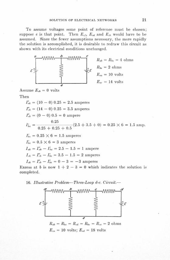
SOLUTION OF ELECTRICAL NETWORKS
To assume voltages some point of reference must be chosen;suppose e is that point. Then Eef, Ed and Eeb would have to beassumed. Since the fewer assumptions necessary, the more rapidlythe solution is accomplished, it is desirable to redraw this circuit asshown with its electrical conditions unchanged.
SAAAAAAA b AAAAAAA C
Rab = Rbc = 4 ohms
Rbe = 2 ohms
Eea = 10 volts
E,, = 14 volts
Assume Eeb = 0 volts
Then
Itb = (10 - 0) 0.25 = 2.5 amperes
Ib = (14 - 0) 0.25 = 3.5 amperes
Ib = (0 - 0) 0.5 = 0 ampere
0.25a = 0.25 + 0.25 + 0.5 (2.5 + 3.5 + 0) = 0.25 X 6 = 1.5 amp.
li = 0.25 X 6 = 1.5 amperes
Ibe = 0.5 X 6 = 3 amperes
Iab = Iab - = 2.5 - 1.5 = 1 ampere
Icb = I-b - = 3.5 - 1.5 = 2 amperes
I b = Ieb - = 0 - 3 = -3 amperes
Excess at b is now 1 + 2 - 3 = 0 which indicates the solution iscompleted.
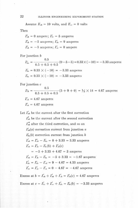
16. Illustrative Problem-Three-Loop d-c. Circuit.-
£ if
Rab = Rbc = Rcd = Rbe = Rce = 2 ohms
Ea = 10 volts; Ed = 18 volts
ILLINOIS ENGINEERING EXPERIMENT STATION
Assume Eb = 10 volts, and Eec = 0 volts
Then
Iab = 0 ampere; Ibc = 5 amperes
Ic = -5 amperes; I'dc = 9 amperes
Ieb = -5 amperes; I', = 0 ampere
For junction b0.5
a 0.5 + 0.5 + 0.5 (0-5-5) =0.33 X(-10) =-3.33 amperes
= 0.33 (-10) = -53.33 amperes
Ibe = 0.33 X (-10) = -3.33 amperes
For junction c0.5
S=0.5 + 0.5 + 0.5 (5 + 9 + 0) = X 14= 4.67 amperes
l'0 = 4.67 amperes
Id = 4.67 amperes
Let lIb be the current after the first correction
Ia"b be the current after the second correction
I'ab after the third correction, and so on
I'b(a) correction current from junction a
Iba(b) correction current from junction b
I'ab = I°ab - Iba = 0 + 3.33 = 3.33 amperes
I'b = Ieb - Ic(b) + Ieb(C)
= -5 + 3.33 + 4.67 = 3 amperes
I'b = Ib - Ie = - 5 + 3.33 = - 1.67 amperes
Idl = Idc - led = 9 - 4.67 = 4.33 amperes
Ie, = I. - Ie = 0 - 4.67 = - 4.67 amperes
Excess at b = l'b + lb + le b = Icb(c) = 4.67 amperes
Excess at c = lie + Ie' + I'c = Ib(b) = -3.33 amperes
SOLUTION OF ELECTRICAL NETWORKS
Second distribution at junction b:
Ia = 0.33 X 4.67 = 1.56 amperes
Ie = 0.33 X 4.67 = 1.56 amperes
IL = 0.33 X 4.67 = 1.56 amperes
Second distribution at junction c:
Ib = 0.33 X (-3.33) = -1.11 amperes
la = 0.33 X (-3.33) = -1.11 amperes
Ie = 0.33 X (-3.33) = -1.11 amperes
Ia"b = b - IL = 3.33 - 1.56 = 1.77 amperes
I"b = Ib - I,(b) + I'b(c)
= 3-1.56 - 1.11 = 0.33 ampere
eb = eb- Ie = -1.67 - 1.56 = -3.23 amperes
Id = Idc- Id = 4.33 + 1.11 = 5.44 amperes
I/c' = ýL - Ie = -4.67 + 1.11 = -3.56 amperes
This process is followed until the accuracy desired is reached, theexcess remaining at each junction being a measure of the accuracyattained. The following tabulation shows the current values aftereach correction. In this case both junctions were corrected, and theresultant conditions were used to recorrect both junctions.
Iab IL le.b Idc Io
Original Values........... 0.0 -5 -5 9 0.01st Correction............ 3.33 3 -1.67 4.33 -4.672nd Correction............ 1.77 0.33 -3.23 5.44 -3.563rd Correction............ 2.15 1.22 -2.86 4.92 -4.084th Correction............ 1.98 0.92 -3.03 5.05 -3.955th Correction............ 2.02 1.02 -2.99 4.99 -4.01
Correct Values............ 2 1 -3 5 -4
In this problem the voltages at b and c were purposely picked atunlikely values, and also were chosen so that a positive excess wouldoriginally exist at junction c and a negative excess at junction b.With such a positive and negative excess at adjacent junctions it isnoticed that the current values found become alternately greater thanand less than their correct value. However, the variation from thetrue value becomes less each time. Reference to this significant fact
ILLINOIS ENGINEERING EXPERIMENT STATION
will be made later, and a method of utilizing it to lessen the workrequired will be suggested.
It is not necessary to correct both or all junctions first and thenfind the new values of the excesses at the junctions. One junctionmay be corrected, the original currents corrected, and the resultantexcess at the adjacent junction distributed and its currents corrected,and so on, treating each junction separately until all have been cor-rected. Returning to the first junction, an excess will be foundbecause of changes at the adjacent junctions. This may be correctedand the same process followed again. This method will be shown inthe following solution of the illustrative problem just solved.
17. Illustrative Problem-Modification of Method Used in Section 16.-
Assume Eeb = 10 volts, Eec = 0 volts as before.
Then Ilb = 0 ampere; Ib = 5 amperes
Icb = -5 amperes; I'cd = 9 amperes
Ioeb = -5 amperes; I°'c = 0 ampere
Excess at junction b = (0 - 5 - 5) = -10 amperes
IHa = 0.33 X (-10) = -3.33 amperes
II = 0.33 X (-10) = -3.33 amperes
Ibc = 0.33 X (-10) = -3.33 amperes
Iab = Iab - Ia = 0 + 3.33 = 3.33 amperes
Ieb = lb - Ie = -5 + 3.33 = -1.67 amperes
Icb = Isb - IL = -5 + 3.33 = -1.67 amperes
Excess at junction c = Ie + I% + I b
= 9 + 0 + 1.67 = 10.67
I'd = 0.33 X 10.67 = 3.56 amperes
Ie = 0.33 X 10.67 = 3.56 amperes
Ib = 0.33 X 10.67 = 3.56 amperes
I'd = Idc - IFd = 9 - 3.56 = 5.44 amperes
lee = I~c - Ie, = 0 - 3.56 = -3.56 amperes
cb = cb + b = - 1.67 + 3.56 = 1.89 amperes
Excess at junction b = I'ab + I'eb + I+"b
= 3.33 - 1.67 + 1.89 = 3.57 amperes
SOLUTION OF ELECTRICAL NETWORKS
This method is followed until the desired accuracy is reached, theexcess remaining at each junction being a measure of the accuracyattained. The following tabulation shows the values of currentexisting after each correction.
Iab Ib Ib I d IOriginal Values ............... 0 -5 -5 9 01st (b) Correction ............. 3.33 -1.67 -1.671st (c) Correction............. 1.89 5.44 -3.562nd (b) Correction............. 2.14 0.70 -2.862nd (c) Correction............. 1.10 5.04 -3.963rd (b) Correction............. 2.01 0.97 -2.993rd (c) Correction ............. 1.01 5.00 -4.004th (b) Correction............. 2.00 1.00 -3.00
Correct Values................ 2 1 -3 5 -4
A comparison of this tabulation with the previous one shows thatthe correct values are reached more rapidly by this process than bythe previous method. This is an advantage, but when many junc-tions are involved it may be found difficult to keep the currents andexcesses at junctions properly tabulated. All currents except thoseat the inlets or outlets of the network will have to be corrected twicewhile going through one cycle of operations.
It has been mentioned previously that all of the excess at ajunction need not be distributed. Only that portion of it, which inthe judgment of the user of the method will cause the desired solutionto occur more rapidly, need be distributed. Conversely, more excessthan actually exists at a junction can also be distributed. The fol-lowing example will serve to illustrate the process followed while usingpartial excesses. This idea may be used in conjunction with eithermethod previously outlined. In the example the method used willbe that first shown.
18. Illustrative Problem-Partial Excess Method.-Still utilizingthe same circuit, assume as before
Eb = 10 volts, Eec = 0 volts.
Then I'b = 0 ampere; I ° = 5 amperes
cb = -5 amperes; I'c = 9 amperes
Ieb = -5 amperes; I'e = 0 ampere
Excess at junction b = (0 - 5 - 5) = -10 amperes
Excess at junction c = (5 + 9 + 0) = 14 amperes
ILLINOIS ENGINEERING EXPERIMENT STATION
Since part of the negative excess at b will appear as a negativeexcess at c after the first correction, and since the same thing willhappen at b as to the positive excess at c, only a partial excess shouldbe distributed at each junction.
Move (-6) at junction b; remainder = -4 amperes
Move (12) at junction c; remainder = +2 amperes
I., = 0.33 X (-6) = -2 amperes
Ie = 0.33 X (-6) = -2 amperes
Iec = 0.33 X (-6) = -2 amperes
led = 0.33 X 12 = 4 amperes
Fe = 0.33 X 12 = 4 amperes
cb = 0.33 X 12 = 4 amperes
Then I',b = Iab -- Ib = 0 + 2 = 2 amperes
Ib b - Ibe = -5 + 2 = -3 amperes
Ib = Ib - I(b) + IWb(C)
= -5+2+4 = 1 ampere
Id = Idc - Ied = 9 - 4 = 5 amperes
I= 4 -- IFe = 0 - 4 = - 4 amperes
Excess at junction b = Ib Ib + I'eb
=2+1-3=0
Excess at junction c = Id + Ibc + IC
=5-1-4=0
This problem is intended only to show the method of procedure,and it is not to be concluded that its use will reduce the number ofoperations necessary to the extent that was possible in this problem.In a network of many junctions it may be difficult to estimate before-hand how much excess will be delivered by adjacent junctions so asto allow the proper amount of excess to remain at the junction underconsideration. After some experience with the method, the user will
SOLUTION OF ELECTRICAL NETWORKS
be able to exercise judgment as to the amount of excess to be dis-tributed at each junction so that a proper solution will result morerapidly.
A more evident advantage in the right to choose the size of excessis the fact that numbers which are more easily handled arithmeticallymay be chosen. An example is the distribution of a partial excessof 10 amperes when the actual excess is 14 amperes. This is particu-larly true when a-c. circuits are involved where both the excesses andthe ratios of distribution appear as complex quantities.
V. SOLUTION OF TYPICAL NETWORK PROBLEM
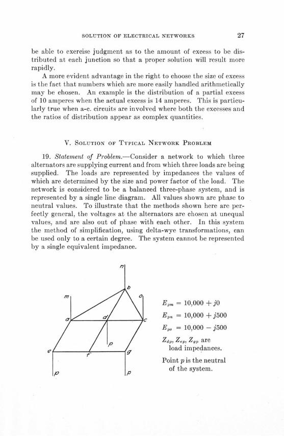
19. Statement of Problem.-Consider a network to which threealternators are supplying current and from which three loads are beingsupplied. The loads are represented by impedances the values ofwhich are determined by the size and power factor of the load. Thenetwork is considered to be a balanced three-phase system, and isrepresented by a single line diagram. All values shown are phase toneutral values. To illustrate that the methods shown here are per-fectly general, the voltages at the alternators are chosen at unequalvalues, and are also out of phase with each other. In this systemthe method of simplification, using delta-wye transformations, canbe used only to a certain degree. The system cannot be representedby a single equivalent impedance.
Epm = 10,000 + jO
Epn = 10,000 + j500
E,o = 10,000 - j500
Zdp, Zep, Zgp areload impedances.
Point p is the neutralof the system.
ILLINOIS ENGINEERING EXPERIMENT STATION
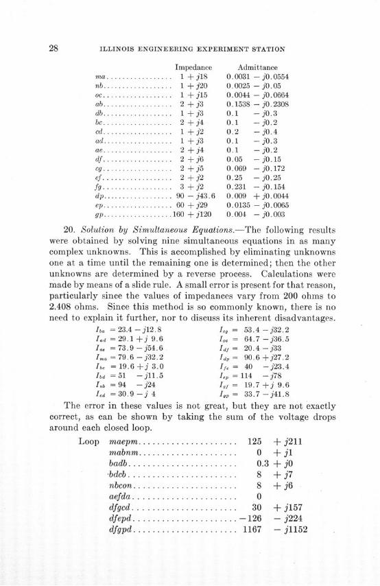
m a . . . . . . . . . . . . . . . . .n b ..................oc . . ... . .. . .. .. .. .. .ab .. ....... ........ .db .. ....... ...... .. .be . . .. .. .. . . .. . ... . .cd . . . ... . .. . .. . .. .. .ad ..................ae ................df ..................cg ..................
ef ................fg . . ..... ........ ..dp ..................ep .. ........ ....... .
Impedance1 + j181 + j201 + j152 + j31 +-j32 + j41 + j21 + j32 + j42 + j62 + j52 + j23 + j2
90 - j43.660 + j29
gp.................. 160 + j120
Admittance0.0031 - j0.05540.0025 - j0.050.0044 - j0.06640.1538 - j0.23080.1 - j0.30.1 - jO.20.2 - jO.40.1 - j0.30.1 - j0.20.05 - jO.150.069 - j0.1720.25 - j0.250.231 - j0.1540.009 + j0.00440.0135 - j0.00650.004 - j0.003
20. Solution by Simultaneous Equations.-The following resultswere obtained by solving nine simultaneous equations in as manycomplex unknowns. This is accomplished by eliminating unknownsone at a time until the remaining one is determined; then the otherunknowns are determined by a reverse process. Calculations weremade by means of a slide rule. A small error is present for that reason,particularly since the values of impedances vary from 200 ohms to2.408 ohms. Since this method is so commonly known, there is noneed to explain it further, nor to discuss its inherent disadvantages.
Iba = 23.4 - j12.8 I, = 53.4 -j32.2Iad = 29.1 +j 9.6 Ioc = 64.7 -- j36.5I, =-73.9--j54.6 Idf = 20.4--j33Ima =79.6--j32.2 Idp = 90.6+j27.2Ibc = 19.6 +j 3.0 If. = 40 -- j23.4Ibd =51 -- 11.5 ,, = 114 --j78In = 94 -- j24 I,f = 19.7 +j 9.6Icd =30.9 -j 4 I,, = 33.7 -- j41.8
The error in these values is not great, but they are not exactlycorrect, as can be shown by taking the sum of the voltage dropsaround each closed loop.
Loop maepm ................... .m abnm .................. ..badb ............. . .......*bdcb ......................nbcon ...... .... .. .......aefda .....................dfgcd.....................dfepd .....................dfgpd .....................
125 + j2110 +jl
0.3 + jO8 +j78 +j6
30.- 126. 1167
+ j157- j224- j1152

SOLUTION OF ELECTRICAL NETWORKS
The large discrepancies are in those loops containing large im-pedances; therefore quite a small error in current values is sufficientto account for such voltage discrepancy.
21. Solution by Balancing Voltage Drops.-In this method it wasthought convenient to use unit or per cent values, since some of theloops involved contain constant voltages independent of impedancedrops. The relationships existing can be shown as follows:
Loop mabnm: ImaZma + IabZab + IbnZbn = Epm, - Epn
Choose a certain current Ir and voltage E, as a basis upon whichto calculate percentage values.
Ima IrZa Iab IrZab Ibn IrZbn Epm - Epn1 r Er Ir Er Ir Er Er
Ima Iab bnr (per cent Zm,) + (per cent Zab) + (per cent Zbn) =
I, Ir Ir
E,, - Ep, X 100
Er
Let Ir = 100 + JO E, = 10,000 + jO
IrZma 100 X 100 X ZmaThen - X 100 = per cent Z,a =
Er 10,000
or per cent Zma = Zma in ohms
Values for Ima/Ir were used as a ratio.
For example, Ima/I, was used as 0.4 + jO
Inb/Ir 0.3 + JO
Ioc/I, 0.3 + JO
The solution by this method was not carried to completion,because it soon became evident that the work involved would bemuch greater than that required by the method of balancing currents.
22. Solution by Balancing Currents.-To solve the network bythis method it is necessary to assume voltage values at each of thejunctions. Any value may be chosen at each point, but an analysis

ILLINOIS ENGINEERING EXPERIMENT STATION
of the network and of the method to be used shows the advantageof choosing the voltage values in a systematic way.
The values of current passing through large impedances will becorrected quite slowly if the other incoming impedances at that junc-tion are small. Since the input and load impedances are all largecompared with the 'grid' impedances, it is desirable to have the inputcurrent total equal the load current total. This may be done byassuming all voltages on the 'grid' to be the same. Then the systemmay be considered merely a single junction into which all alternatorsfeed, and from which all loads are supplied. Then, by assuming avoltage at this single junction, calculating the currents, finding theexcess, and distributing it once, the values of current in each alterna-tor and load are found. The resulting values will be such that thetotal current entering the system will equal the total current leavingit. This preliminary method is worthy of consideration, since it willshorten the calculation, and applies to the usual a-c. power network.
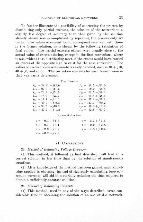
When the currents are thus determined the original network isconsidered. Excesses will result at a, b, c, d, e, and g. These excesseswill be positive at a, b, and c and negative at d, e, and g. Each junc-tion is treated, the new excesses found, these distributed, and so on,until the excesses at each point are small enough to indicate that thesolution is sufficiently accurate. The final currents, found after thefifteenth correction, are shown in the following tabulation.
Final results
Ib, = 24.1 -j11.4 Il, = 40.4 -j31.7
Iad = 26.6 +j11.0 loc = 59.6 -j30.7
I., = 74.6 -j 50.7 Idf = 25.4 - j29.4I~ = 76.2 - j27.2 Idp = 91.1 + j29.7I,& = 17.4 -j 0.7 If, = 36.2 - j28.5Ibd = 50.3 -j 8.7 ,,p = 112.6 -j80.2
Inb = 90.7 -j19.6 I,, = 9.8 +j 1.5
led = 37.5 -j 1.0 I,, = 33.4 -j33.6
Excess at Junction
a= 0.9+jl.1 e = -1.8 +j 1.0
b = -1.1 +jO.8 f = -1.0 +j 0.6
c = -0.9 +j1.3 g= -2.8-j 0.4
d = -2.1 +j1.0
To illustrate how, after the first corrections, the currents becometoo large and then too small, each time differing from the correctvalue by a smaller amount, the following curve sheets (Figs. 1, 2,

SOLUTION OF ELECTRICAL NETWORKS
K
ix
I..-K
92 Rea/ Coponent - I
Snd4, //t, etc. Approw/dnate Currents
l 3rd etc. Appro/wmate Currents
/mag/nary Component -S-na, 4th etc. Appr'/ate Currents_
S ' , 3rd etc. Apprne Curren
SI 3 4 5 6 7 8 9 10 /I /2 13 14 15Number of Correct/ons
FIG. 1. ENVELOPE CURVE FOR APPROXIMATIONS-LOAD CURRENT
64------------X-----------643 \ / /maReal Component--
S4th, et nl. 4Ah, etc. Arppro tee CurCurrreen
,s60 3r-_ etc. Approx'-e Currents
-" -/s-, 3nf, etc. Approx. Currenes
3Z I _ /nay Component-INt\ --tnd, 4h etc. Approximate Currents
/^ ^ ____. *^'i'^l/t, 3rd, etc. Approximate Curet
ix
KK
/ 2 3 4 6 6 7 8 9 10 /I /2 13 14 S/Number of Correcf/ons
FIG. 2. ENVELOPE CURVE FOR APPROXIMATIONS-INPUT CURRENT

ILLINOIS ENGINEERING EXPERIMENT STATION
(j~
1~
(2
80
?0
60
50
40
/
-7
•» ---. s•;_-? 3rd, e^l. Approx. Currewfs-
\\ ii \\ i/ .- / ^~-\
\ • I^ "^' 'ncf 4t/h, e/c. Approximatq e
/' mag/n~ar 2 Compon~ u ien • - -
\ •"''^' •/st, 3rd etc. Approx. Currents --~zjN
7
0 /I 3 4 5 6 7 8 9 /I// /2 /3 /4 /5Number of Correct/ons
FIG. 3. ENVELOPE CURVE FOR APPROXIMATIONS-NETWORK CURRENT
and 3) show the envelope curves of three typical currents, namely, aload current (Fig. 1), an input current (Fig. 2), and a line or networkcurrent (Fig. 3). Plotting the values of any other current will resultin curves having the same characteristics. One of the curves on thecurve sheet is the real component of the first, third, etc., approximatecurrents. The companion cuive is that of the real components ofthe second, fourth, etc., approximate currents. The imaginary com-ponents of the current are treated in like fashion, resulting in similarenvelope curves. In this solutioh, total excesses were distributedeach time.
The purpose of including these envelope curves is to show that,if total excesses are distributed as was done in this solution, theenvelope curves for any other problem could be drawn as the solutionproceeds and, if only reasonable accuracy is required, the currents ineach branch could be found by extrapolation, thereby shortening thecalculation considerably. It is interesting to note that in this particu-lar solution the center point between the envelope curves at the sixthapproximation is in each case within one ampere of the finally-deter-mined value. This was found to be true for all values of current inthe network. In some instances it differed from the proper value byless than one ampere. This applies to both the real and the imaginarycomponents.
~1~I
1-
4-
'ný7d 4h, ec. Aoprox/ma'<e Currents
Li
% i # •1 • - , 4 ¢
21nI
I
SOLUTION OF ELECTRICAL NETWORKS
To further illustrate the possibility of shortening the process bydistributing only partial excesses, the solution of the network to aslightly less degree of accuracy than that given by the solutionalready shown was accomplished by repeating the process only sixtimes. The values of current found correspond very well with thosein the former solution, as is shown by the following tabulation offinal values. The partial excesses chosen were usually close to theactual value of excess existing, except in the first corrections, whereit was evident that distributing most of the excess would have causedan excess of the opposite sign to exist for the next correction. Thevalues of excess chosen were numbers easily handled, such as 10 + jl0,40 + jO, and so on. The correction currents for each branch were inthat way easily determined.
Final Results
Iba = 24.31 - j12.6 I,, = 38.5 -j32.0lad = 27.0 +j11.5 1oc = 59.2 -j28.8Ia, =73.2 -j51.5 Idf= 23.5-j30.2I,= 75.9 -j25.7 Idp = 91.4 + j28.4Ibc = 17.1 -j 1.1 If = 37.2 -j25.2Ibd = 49.9 -j 9.5 I,, =113.1 -j80.2
,,b =90.5 -j18.2 I,, = 10.8+j 1.2Icd =37.7 -j 1.2 1,p = 32.5 -j33.7
Excess at Junction
a =-0.1 +1.6 e = -2.7+j 3.6
b = -0.7 +j 5.1 f = -2.9 -j 3.8
c = -2.9+j3.2 g = -4.8 +j 0.5
d = -0.2+1j2.6
VI. CONCLUSIONS
23. Method of Balancing Voltage Drops.-
(1) This method, if followed as first described, will lead to acorrect solution in less time than by the solution of simultaneousequations.
(2) After knowledge of the method has been gained, such knowl-edge applied in choosing, instead of rigorously calculating, loop cor-rection currents, will aid in materially reducing the time required toobtain a sufficiently accurate solution.
24. Method of Balancing Currents.-
(1) This method, used in any of the ways described, saves con-siderable time in obtaining the solution of an a-c. or d-c. network.
ILLINOIS ENGINEERING EXPERIMENT STATION
(2) After knowledge of the method has been gained, the distri-bution of partial excesses will cause the desired solution to resultquite rapidly.
(3) If total excesses are distributed in each case, the envelopecurves may be drawn as the solution proceeds, and the necessity foradditional work will be told visually by those curves. Extrapolationof the curves, or midpoints between the two pairs of curves, may beused to determine current values if extreme accuracy is not essential.
(4) If the solution is set up in proper form the method becomesvery simple, and there is little chance for error. Appendix A showssuggested forms that may prove useful.
(5) If an error exists in the solution finally obtained, it will becomeevident by checking voltages at each junction as obtained by arrivingat the junction over the various possible paths. If discrepanciesarise, choose the most logical value of voltage at that junction. Bydoing that for each junction, and calculating resultant branch cur-rents, excesses of an order dependent upon the size of the error willappear. These excesses can soon be distributed properly. It is notnecessary to begin the solution all over again.
(6) If a change is contemplated in a present network for which asolution has been obtained previously, the solution of the new net-work can be obtained readily by merely introducing the excess causedby the change, and proceeding from that point.
For example, if a load is to be added at point a, assume that thevoltage is that value present on the actual system, and a negativeexcess at that point will appear due to the added load. Distributionof that excess will require less time than if an entirely new solutionwere required. In the same way an alternator added to the systemwill cause a positive excess, which may be given the usual treatment.If a line is added between junctions a and b, the existing voltages ofthe actual system will cause excesses at points a and b, one positiveand the other negative. Proceeding from this starting point, asatisfactory solution will soon result.
Neither of the two methods here described has been fully explored.In the particular field considered, a-c. power networks, the methods,particularly the second one described, have considerable merit. Thesame principles will apply equally well in other particular types ofcircuits, and the user will soon gain the experience necessary to makethe methods even more helpful.

SOLUTION OF ELECTRICAL NETWORKS
APPENDIX A
1. Suggested Forms.-It is desirable to use some definite method oftabulating the calculations necessary in employing any of the methodsset forth in this bulletin. The ingenuity and individual taste of theoperator will determine the method of tabulation. Any method whichwill decrease the errors of omission and facilitate numerical calcula-tions will prove worthy of adoption. The following form is sug-gested as such a method when a solution by balancing currents isbeing obtained.
A sheet, laid out as shown in the following, should be utilized foreach junction, each sheet being given the same index letter as thejunction on the network diagram. Calculations of successive correc-tion currents are made on each sheet and, by reference to the othersheets, the excesses may be found and recorded for each junction.
Consider a network a part of which consists of a junction a con-nected to junction b through Yba, to junction c through Yea, and tojunction d through Yda. Similar conditions will exist at junctions b,c, d, and all other junctions of the network, but consideration ofjunction a will show the method of setting up the forms for theother junctions.
YbaIeb = DabNa where Dab = -
K
YeaIac = DacNa where Dac = -
K
YdaIad = DadNa where Dad =-
K
Na = excess to be distributed from junction a
K = Yba + Yea + Yda
X'i = Ia(b) + I1.(c) + Ida(d)
Ila(b) is Iba from sheet B
Ica(C) is Iea from sheet C
Ida(d) is Ida from sheet D
Let N' = X: - R:
Na = Xa + Ra - Re
'N" = X" +R - R

ILLINOIS ENGINEERING EXPERIMENT STATION
These results may be shown on a sheet of the following form:
ACorrection Correction Correction Excess
a to b a to c a to d Iia(b)IWb(a) I'(a) Icd(a) + I•(c)
Db Dc Dad +I'a (d)+ Remainder
N °
DbN° DacN? D.adNN.
D.bN' DN'aN DaaN'
Multiplications involved may be checked each time, since DabN +DacN + D,adN = N.
Then final current values may be found as illustrated here for lab;
lab = IFb + VI:b(a) - IZa(b)
Illustration of Sheet A
Assume junction a is connected to junctions b, c, and d throughimpedances Zab, Zac, and Zad.
Let Yab = 0.25 - jO.25
Yac = 0.05 - j0.15
Yad = 0.2308 - j0.1538
K = 0.5308 - j0.5538
YabDa = -- = 0.461 + j0.010
KYac
Da = - = 0.188 - j0.088KYad
Dad = - = 0.351 + j0.078K
Check 1.000 + JO
Let assumed voltages be such that
Iab = 40 + j20
I'a = 20 - j45
I oad = -80 + j5
X = Ioa + Ic•+ ~ = 20 + j20
SOLUTION OF ELECTRICAL NETWORKS
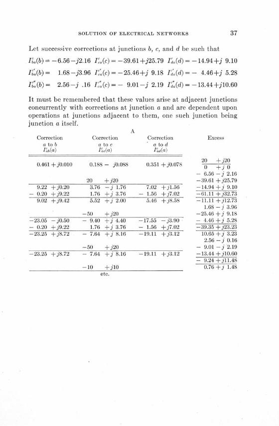
Let successive corrections at junctions b, c, and d be such that
Ia(b) - -6.56-j2.16 I"a(c) = -39.61+j25.79 Ida(d) = - 14.94+j 9.10
Iba(b)= 1.68 -j3.96 I'a(c)= -25.46+j 9.18 I'Jd(d) = - 4.46+j 5.28
Ibi(b)= 2.56-j .16 Ica(c) = - 9.01-j 2.19 I7"(d) =-13.44+jl10.60
It must be remembered that these values arise at adjacent junctionsconcurrently with corrections at junction a and are dependent uponoperations at junctions adjacent to them, one such junction beingjunction a itself.
Correctiona to bI'b(a)
Correctiona to ca,(a)
Correctiona to dId(a)
0.461 +j0.010 0.188 - j0.088 0.351 +j0.078
20 + j209.22 +j0.20 3.76 - j 1.76 7.02 +jl.56
- 0.20 +j9.22 1.76 + 3.76 - 1.56 + j7.029.02 + j9.42 5.52 +j 2.00 5.46 +J8.58
-50 + j20-23.05 -j0.50 - 9.40 + 4.40 -17.55 -j3.90- 0.20 + j9.22 1.76 + j 3.76 - 1.56 + j7.02-23.25 +j8.72 - 7.64 + j 8.16 -19.11 +j 3 .12
-50 + j20-23.25 + j8.72 - 7.64 +j 8.16 -19.11 + j 3 .12
-10 +l10etc.
Excess
20 + j200 +j 0
- 6.56 -j 2.16-39.61 + j25.79-14.94 +j 9.10-61.11 + j32.73-11.11 + j12.73
1.68 - j 3.96-25.46 +j 9.18- 4.46 +j 5.28-39.35 + j23.23
10.65 +j 3.232.56 - j 0.16
- 9.01 -j 2.19-13.44 + j10.60- 9.24 + j11.48
0.76 +j 1.48
ILLINOIS ENGINEERING EXPERIMENT STATION
APPENDIX B
BIBLIOGRAPHY
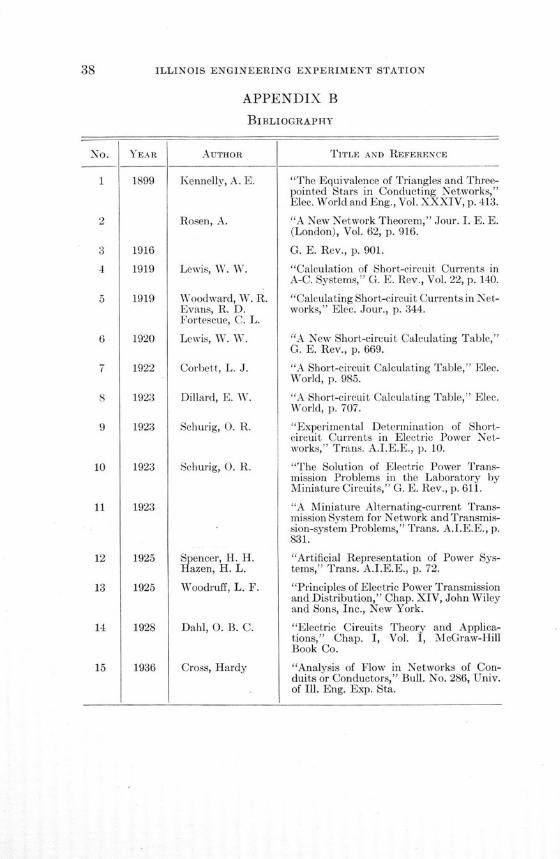
No. YEAR AUTHOR
Kennelly, A. E.
Rosen, A.
Lewis, W. W.
Woodward, W. R.Evans, R. D.Fortescue, C. L.
Lewis, W. W.
Corbett, L. J.
Dillard, E. W.
Schurig, 0. R.
Schurig, 0. R.
Spencer, H. H.Hazen, H. L.
Woodruff, L. F.
Dahl, 0. B. C.
Cross, Hardy
TITLE AND REFERENCE
"The Equivalence of Triangles and Three-pointed Stars in Conducting Networks,"Elec. World and Eng., Vol. XXXIV, p. 413.
"A New Network Theorem," Jour. I. E. E.(London), Vol. 62, p. 916.
G. E. Rev., p. 901.
"Calculation of Short-circuit Currents inA-C. Systems," G. E. Rev., Vol. 22, p. 140.
"Calculating Short-circuit Currents in Net-works," Elec. Jour., p. 344.
"A New Short-circuit Calculating Table,"G. E. Rev., p. 669.
"A Short-circuit Calculating Table," Elec.World, p. 985.
"A Short-circuit Calculating Table," Elec.World, p. 707.
"Experimental Determination of Short-circuit Currents in Electric Power Net-works," Trans. A.I.E.E., p. 10.
"The Solution of Electric Power Trans-mission Problems in the Laboratory byMiniature Circuits," G. E. Rev., p. 611.
"A Miniature Alternating-current Trans-mission System for Network and Transmis-sion-system Problems," Trans. A.I.E.E., p.831.
"Artificial Representation of Power Sys-tems," Trans. A.I.E.E., p. 72.
"Principles of Electric Power Transmissionand Distribution," Chap. XIV, John Wileyand Sons, Inc., New York.
"Electric Circuits Theory and Applica-tions," Chap. I, Vol. I, McGraw-HillBook Co.
"Analysis of Flow in Networks of Con-duits or Conductors," Bull. No. 286, Univ.of Ill. Eng. Exp. Sta.

RECENT PUBLICATIONS OFTHE ENGINEERING EXPERIMENT STATIONt
Circular No. 23. Repeated-Stress (Fatigue) Testing Machines Used in theMaterials Testing Laboratory of the University of Illinois, by Herbert F. Mooreand Glen N. Krouse. 1934. Forty cents.
Bulletin No. 266. Investigation of Warm-Air Furnaces and Heating Systems,Part VI, by Alonzo P. Kratz and Seichi Konzo. 1934. One dollar.
Bulletin No. 267. An Investigation of Reinforced Concrete Columns, by FrankE. Richart and Rex L. Brown. 1934. One dollar.
Bulletin No. 268. The Mechanical Aeration of Sewage by Sheffield Paddles andby an Aspirator, by Harold E. Babbitt. 1934. Sixty cents.
Bulletin No. 269. Laboratory Tests of Three-Span Reinforced Concrete ArchRibs on Slender Piers, by Wilbur M. Wilson and Ralph W. Kluge. 1934. One dollar.
Bulletin No. 270. Laboratory Tests of Three-Span Reinforced Concrete ArchBridges with Decks on Slender Piers, by Wilbur M. Wilson and Ralph W. Kluge.1934. One dollar.
Bulletin No. 271. Determination of Mean Specific Heats at High Temperaturesof Some Commercial Glasses, by Cullen W. Parmelee and Alfred E. Badger. 1934.Thirty cents.
Bulletin No. 272. The Creep and Fracture of Lead and Lead Alloys, by HerbertF. Moore, Bernard B. Betty, and Curtis W. Dollins. 1934. Fifty cents.
Bulletin No. 273. Mechanical-Electrical Stress Studies of Porcelain InsulatorBodies, by Cullen W. Parmelee and John 0. Kraehenbuehl. 1935. Seventy-five cents.
Bulletin No. 274. A Supplementary Study of the Locomotive Front End byMeans of Tests on a Front-End Model, by Everett G. Young. 1935. Fifty cents.
Bulletin No. 275. Effect of Time Yield in Concrete upon Deformation Stressesin a Reinforced Concrete Arch Bridge, by Wilbur M. Wilson and Ralph W. Kluge.1935. Forty cents.
Bulletin No. 276. Stress Concentration at Fillets, Holes, and Keyways as Foundby the Plaster-Model Method, by Fred B. Seely and Thomas J. Dolan. 1935.Forty cents.
Bulletin No. 277. The Strength of Monolithic Concrete Walls, by Frank E.Richart and Nathan M. Newmark. 1935. Forty cents.
Bulletin No. 278. Oscillations Due to Corona Discharges on Wires Subjectedto Alternating Potentials, by J. Tykocinski Tykociner, Raymond E. Tarpley, andEllery B. Paine. 1935. Sixty cents.
Bulletin No. 279. The Resistance of Mine Timbers to the Flow of Air, asDetermined by Models, by Cloyde M. Smith. 1935. Sixty-five cents.
Bulletin No. 280. The Effect of Residual Longitudinal Stresses upon the Load-carrying Capacity of Steel Columns, by Wilbur M. Wilson and Rex L. Brown. 1935.Forty cents.
Circular No. 24. Simplified Computation of Vertical Pressures in ElasticFoundations, by Nathan M. Newmark. 1935. Twenty-five cents.
Reprint No. 3. Chemical Engineering Problems, by Donald B. Keyes. 1935.Fifteen cents.
Reprint No. 4. Progress Report of the Joint Investigation of Fissures in Rail-road Rails, by Herbert F. Moore. 1935. None available.
Circular No. 25. Papers Presented at the Twenty-Second Annual Conferenceon Highway Engineering, Held at the University of Illinois, Feb. 21 and 22, 1935.1936. Fifty cents.
Reprint No. 5. Essentials of Air Conditioning, by Maurice K. Fahnestock.1936. Fifteen cents.
Bulletin No. 281. An Investigation of the Durability of Molding Sands, byCarl H. Casberg and Carl E. Schubert. 1936. Sixty cents.
Bulletin No. 282. The Cause and Prevention of Steam Turbine Blade Deposits,by Frederick G. Straub. 1936. Fifty-five cents.
tCopies of the complete list of publications can be obtained without charge by addressing theEngineering Experiment Station, Urbana, Ill.
40 ILLINOIS ENGINEERING EXPERIMENT STATION
Bulletin No. 283. A Study of the Reactions of Various Inorganic and OrganicSalts in Preventing Scale in Steam Boilers, by Frederick G. Straub. 1936. One dollar.
Bulletin No. 284. Oxidation and Loss of Weight of Clay Bodies During Firing,by William R. Morgan. 1936. Fifty cents.
Bulletin No. 285. Possible Recovery of Coal from Waste at Illinois Mines, byCloyde M. Smith and David R. Mitchell. 1936. Fifty-five cents.
Bulletin No. 286. Analysis of Flow in Networks of Conduits or Conductors,by Hardy Cross. 1936. Forty cents.
Circular No. 26. Papers Presented at the First Annual Conference on AirConditioning, Held at the University of Illinois, May 4 and 5, 1936. Fifty cents.
Reprint No. 6. Electro-Organic Chemical Preparations, by S. Swann, Jr. 1936.Thirty-five cents.
Reprint No. 7. Papers Presented at the Second Annual Short Course in CoalUtilization, Held at the University of Illinois, June 11, 12, and 13, 1935. 1936.None available.
Bulletin No. 287. The Biologic Digestion of Garbage with Sewage Sludge, byHarold E. Babbitt, Benn J. Leland, and Fenner H. Whitley, Jr. 1936. One dollar.
Reprint No. 8. Second Progress Report of the Joint Investigation of Fissuresin Railroad Rails, by Herbert F. Moore. 1936. Fifteen cents.
Reprint No. 9. Correlation Between Metallography and Mechanical Testing,by Herbert F. Moore. 1936. None available.
Circular No. 27. Papers Presented at the Twenty-Third Annual Conferenceon Highway Engineering, Held at the University of Illinois, Feb. 26-28, 1936. 1936.Fifty cents.
Bulletin No. 288. An Investigation of Relative Stresses in Solid Spur Gears bythe Photoelastic Method, by Paul H. Black. 1936. Forty cents.
Bulletin No. 289. The Use of an Elbow in a Pipe Line for Determining the Rateof Flow in the Pipe, by Wallace M. Lansford. 1936. Forty cents.
Bulletin No. 290. Investigation of Summer Cooling in the Warm-Air HeatingResearch Residence, by Alonzo P. Kratz, Maurice K. Fahnestock, and Seichi Konzo.1937. One dollar.
Bulletin No. 291. Flexural Vibrations of Piezoelectric Quartz Bars and Plates,by J. Tykocinski Tykociner and Marion W. Woodruff. 1937. Forty-five cents.
Reprint No. 10. Heat Transfer in Evaporation and Condensation, by MaxJakob. 1937. Thirty-five cents.
*Circular No. 28. An Investigation of Student Study Lighting, by John 0.Kraehenbuehl. 1937. Forty cents.
*Circular No. 29. Problems in Building Illumination, by John 0. Kraehenbuehl.1937. Thirty-five cents.
*Bulletin No. 292. Tests of Steel Columns; Thin Cylindrical Shells; LacedChannels; Angles, by Wilbur M. Wilson. 1937. Fifty cents.
*Bulletin No. 293. The Combined Effect of Corrosion and Stress Concentrationat Holes and Fillets in Steel Specimens Subjected to Reversed Torsional Stresses,by Thomas J. Dolan. 1937. Fifty cents.
*Bulletin No. 294. Tests of Strength Properties of Chilled Car Wheels, byFrank E. Richart, Rex L. Brown, and Paul G. Jones. 1937. Eighty-five cents.
*Bulletin No. 295. Tests of Thin Hemispherical Shells Subjected to InternalHydrostatic Pressure, by Wilbur M. Wilson and Joseph Marin. 1937. Thirty-five cents.
Circular No. 30. Papers Presented at the Twenty-fourth Annual Conference onHighway Engineering, Held at the University of Illinois, March 3-5, 1937. 1937.None available.
*Bulletin No. 296. Magnitude and Frequency of Floods on Illinois Streams, byGeorge W. Pickels. 1937. Seventy cents.
*Bulletin No. 297. Ventilation Characteristics of Some Illinois Mines, by CloydeM. Smith. 1937. Seventy cents.
*Bulletin No. 298. Resistance to Heat Checking of Chilled Iron Car Wheels,and Strains Developed Under Long-continued Application of Brake Shoes, by EdwardC. Schmidt and Herman J. Schrader. 1937. Fifty-five cents.
*Bulletin No. 299. Solution of Electrical Networks by Successive Approxima-tions, by Laurence L. Smith. 1937. Forty-five cents.
*A limited number of copies of bulletins starred are available for free distribution.
UNIVERSITY OF ILLINOIS
Colleges and Schools at UrbanaCOLLEGE OF LIBERAL ARTS AND SCIENCES.-General curriculum with majors in the hu-
manities and sciences; specialized curricula in chemistry and chemical engineering;general courses preparatory to the study of law and journalism; pre-professionaltraining in medicine, dentistry, and pharmacy.
COLLEGE OF COMMERCE AND BUSINESS ADMINISTRATION.-Curricula in general business,trade and civic secretarial service, banking and finance, insurance, accountancy,transportation, commercial teaching, foreign commerce, industrial administration,public utilities, and commerce and law.
COLLEGE OF ENGINEERING.-Curricula in agricultural engineering, ceramics, ceramic en-gineering, chemical engineering, civil engineering, electrical engineering, engineer-ing physics, general engineering, mechanical engineering, metallurgical engineering,mining engineering, and railway engineering.
COLLEGE OF AGRICULTURE.-Curricula in agriculture, floriculture, general home econom-ics, and nutrition and dietetics.
COLLEGE OF EDUCATION.-Curricula in education, agricultural education, home econom-ics education, and industrial education. The University High School is the practiceschool of the College of Education.
COLLEGE OF FINE AND APPLIED ARTS.-Curricula in architecture, landscape architecture,music, and painting.
COLLEGE OF LAW.-Professional curriculum in law.SCHOOL OF JOURNALISM.-General and special curricula in journalism.SCHOOL OF PHYSICAL EDUCATION.-Curricula in physical education for men and for
women.LIBRARY SCHooL.-Curriculum in library science.GRADUATE SCHooL.-Advanced study and research.
University Extension Division.-For a list of correspondence courses conductedby members of the faculties of the colleges and schools at Urbana and equiva-lent to courses offered to resident students, address the Director of the Divisionof University Extension, 109 University Hall, Urbana, Illinois.
Colleges in Chicago
COLLEGE OF MEDICINE.-Professional curriculum in medicine.COLLEGE OF DENTISTRY.-Professional curriculum in dentistry.COLLEGE OF PHARMACY.-Professional curriculum in pharmacy.
University Experiment Stations, and Research andService Bureaus at Urbana
AGRICULTURAL EXPERIMENT STATION BUREAU OF BUSINESS RESEARCH
ENGINEERING EXPERIMENT STATION BUREAU OF COMMUNITY PLANNING
EXTENSION SERVICE IN AGRICULTURE BUREAU OF EDUCATIONAL RESEARCH
AND HOME ECONOMICS BUREAU OF INSTITUTIONAL RESEARCH
State Scientific Surveys and Other Divisions at UrbanaSTATE GEOLOGICAL SURVEY STATE DIAGNOSTIC LABORATORY
STATE NATURAL HISTORY SURVEY (Animal Pathology)STATE WATER SURVEY UNITED STATES WEATHER BUREAU
STATE HISTORICAL SURVEY STATION
For general catalog of the University, special circulars, and other information, address
THE REGISTRAR, UNIVERSITY OF ILLINOIS
URBANA, ILLINOIS