Solutions to Problems for 2D & 3D Heat and Wave

Equations

18.303 Linear Partial Differential Equations

Matthew J. Hancock

1 Problem 1

A rectangular metal plate with sides of lengths L, H and insulated faces is heated to a

uniform temperature of u0 degrees Celsius and allowed to cool with three of its edges

maintained at 0o C and the other insulated. You may use dimensional coordinates,

with PDE

ut = κ∇ 2 u, 0 ≤ x ≤ L, 0 ≤ y ≤ H.

The BCs are

∂u u (0, y, t) = 0 = u (L, y, t) , u (x, 0, t) = 0, (x,H, t) = 0. (1)

∂y

(i) Solve for u (x, y, t) subject to an initial condition u (x, y, 0) = 100.

(ii) Find the smallest eigenvalue λ and the first term approximation (i.e. the term

with e−λκt).

(iii) For fixed t = t0 ≫ 0, sketch the level curves u = constant as solid lines and

the heat flow lines as dotted lines, in the xy-plane.

(iv) Of all rectangular plates of equal area, which will cool the slowest? Hint: for

each type of plate, the smallest eigenvalue gives the rate of cooling.

(v) Does a square plate, side length L, subject to the BCs (1) cool more or less

rapidly than a rod of length L, with insulated sides, and with ends maintained at 0o

C? You may use the results we derived in class for the rod, without derivation.

Solution: (i) We separate variables as

u (x, y, t) = v (x, y) T (t)

1

Fall 2006

to obtain T ′ 2v

= (2) κT

= ∇v

−λ

where λ is constant since the l.h.s. depends only on t and the middle depends only

on (x, y). We so obtain the Sturm-Liouville problem

2 ∇ v + λv = 0 (3)

The BCs are

∂v v (0, y) = 0 = v (L, y) , v (x, 0) = 0, (x,H) = 0. (4)

∂y

Separating variables again for v (x, y) gives

v (x, y) = X (x) Y (y) (5)

and substituting into the PDE (3) gives

X ′′Y + XY ′′ + λ = 0

Rearranging gives Y ′′ X ′′

+ λ = = µ (6) Y

−X

where µ is constant because the l.h.s. depends only on y and the middle on x.

Introducing (5) into the BCs (4) gives

0 = v (0, y) = X (0) Y (y) X (0) = 0⇒ 0 = v (L, y) = X (L) Y (y) X (L) = 0⇒ 0 = v (x, 0) = X (x) Y (0) Y (0) = 0⇒

∂v 0 = (x,H) = X (x) Y ′ (H) Y ′ (H) = 0

∂y ⇒

We begin with the problem for X (x), since we have a complete set (two) of

homogeneous Type I BCs, the simplest to deal with. From (6), the ODE for X (x) is

X ′′ + µX = 0; X (0) = 0 = X (L)

We’ve seen before that the eigenfunctions and eigenvalues are

� nπx � n2π2

Xn (x) = sin L

, µn = L2

, n = 1, 2, 3...

From (6), with µ = µn, the ODE for Y (y) is

Y ′′ + νY = 0; Y (0) = 0 = Y ′ (H)

2

� �

�

�� � �

� �� � �

� � � � �

� � � � �

� �

� �� � �

� � � �

where ν = λ − µn. Again, we’ve seen ODEs like this before, that ν > 0 and

Y (y) = A cos �√

vy + B sin �√

vy

Imposing the BCs gives

0 = Y (0) = A

0 = Y ′ (H) = B√

v cos �√

vH

Note that B cannot be zero since we desire a non-trivial solution. Hence cos (√

vH) =

0 and � �

1√vH = m + π, m = 1, 2, 3...

2

Thus the eigenvalues and eigenfunctions are

� �21 π2

vm = m −2 H2

, m = 1, 2, 3...

1 yYm (y) = sin m − π

2 H

The general solution to the Sturm-Liouville problem for v (x, y) is

� nπx 1 y vmn (x, y) = sin sin m − π , n,m = 1, 2, 3...

L 2 H

From (2), the solution for T (t) is

1 �2

1 n2

T = e−κλt = e−κ(νm+µn)t = exp m − + κπ2t− 2 H2 L2

The general solution to the PDE and BCs for u (x, y, t) is

�� � � � � nπx 1 y 1

�2 1 n2

umn (x, y, t) = sin sin m − π exp m − + L 2 H

− 2 H2 L2

κπ2t ,

for n,m = 1, 2, 3... To satisfy the initial condition, we use superposition and sum over

all m, n to obtain

∞ ∞

u (x, y, t) = umn (x, y, t)m=1 n=1∞ ∞�� � nπx 1 y

= Amn sin sin m − π L 2 H

m=1 n=1 � �2

1 1 n2

· exp m − + κπ2t− 2 H2 L2

3

� �� � �

�� � �

� �� � �

� � � �

� � � �

� �

� � � �

� � �

To find the constants Amn, we impose the IC:

∞ ∞�� � nπx 1 y

100 = u (x, y, 0) = Amn sin sin m − π L 2 H

m=1 n=1

Using orthogonality relations for sin, we have

4 � L � H �� nπx 1 y

100 sin sin m − π dydx Amn = LH 0 L 2 H0

� H400 � L � nπx 1 y

= sin dx sin m − π dy LH 0 L 2 H0

� �� � � � 400 L 2H 1

= (cos (nπ) − 1)(2m − 1) π

cos m − π − 1 LH nπ 2

800 = )

n (2m − 1) π2 (1 − (−1)n

Thus Am2n = 0 and 1600

=Am2n−1 (2n − 1) (2m − 1) π2

and

∞�� 1600 (2m − 1) πy

u (x, y, t) = ∞

sin (2n − 1) πx

sin (2n − 1) (2m − 1) π2 L 2H

m=1 n=1

2 2(2m − 1) (2n − 1)· exp − 4H2

+ κπ2t L2

(ii) The smallest eigenvalue λ is

1 1 π2λ11 = +

4H2 L2

and the first term approximation is

� � � 1 11600 � πx πy u (x, y, t) ≈ u11 (x, y, t) = sin sin + κπ2t

π2 L 2H exp −

4H2 L2

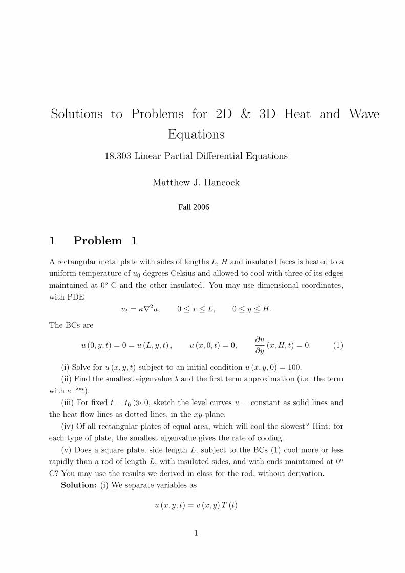
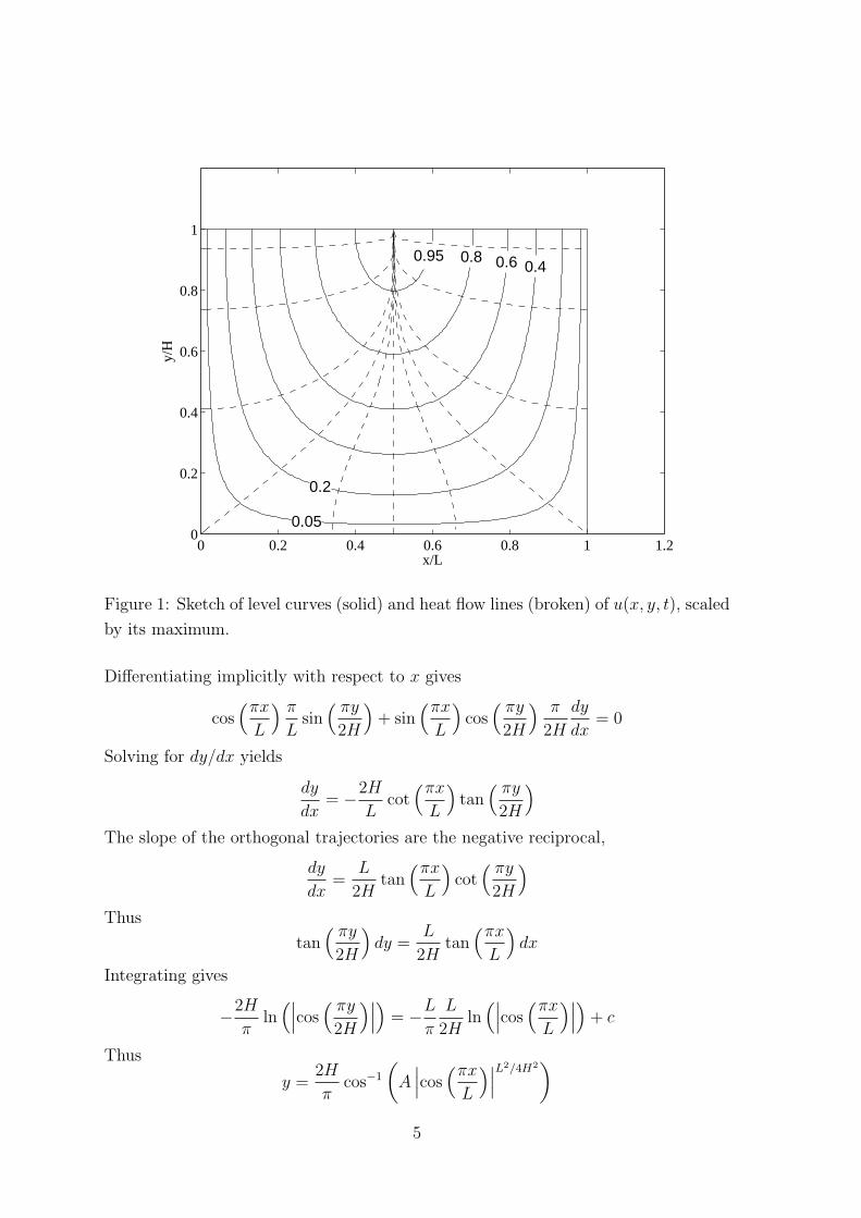
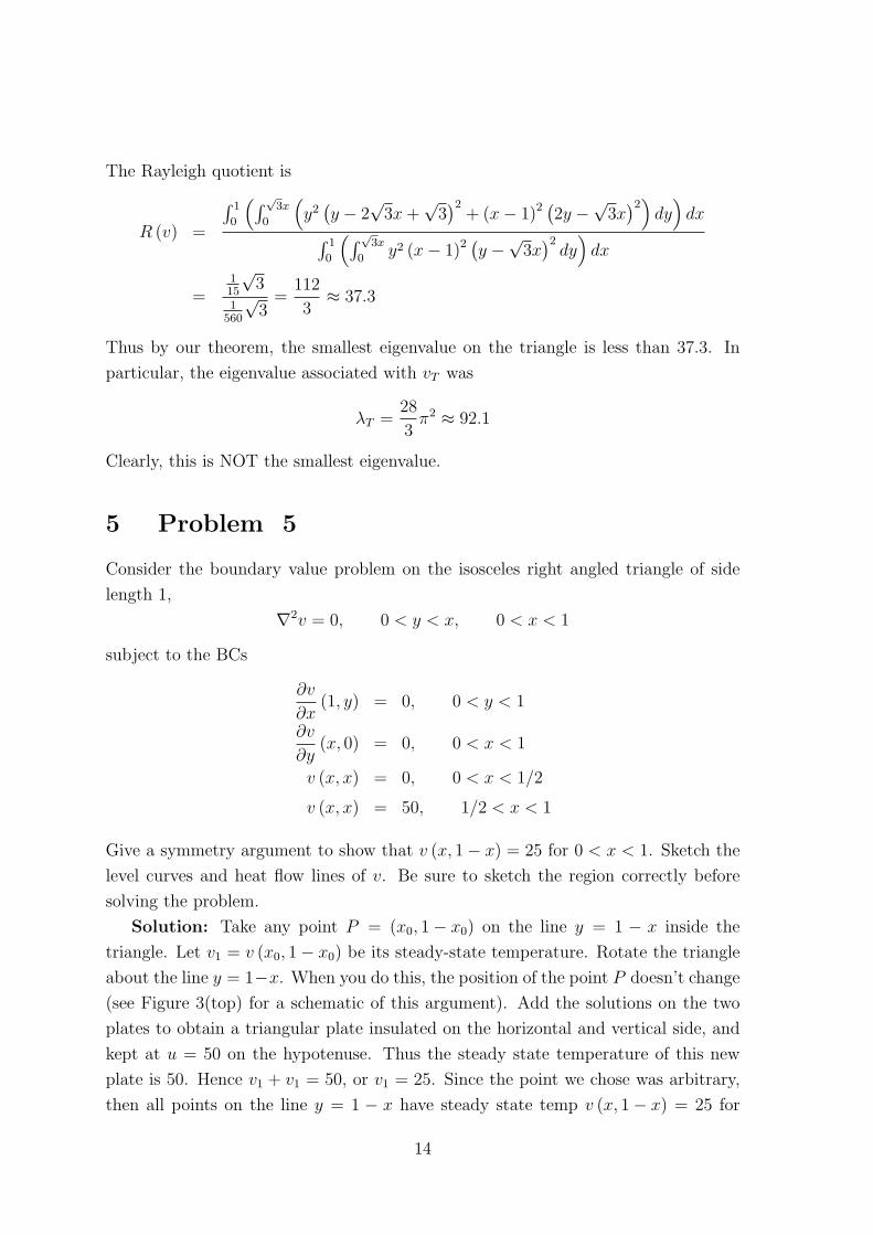
(iii) To draw the level curves, note that the isotherms (lines of constant temp,

i.e. level curves) will intersect the insulated side (y = H) at right angles, and cannot

intersect the other sides, which are also isotherms (u = 0). Using these constraints

and continuity allow you to sketch the curves. The level curves and heat flow lines

are plotted as solid and dotted lines, respectively, in Figure 1.

[extra] The heat flow lines are found by finding the orthogonal trajectories to the

level curves � πx πy

sin sin = c L 2H

4

� � �

� � �

� =

y/H

1

0.8

0.6

0.4

0.2

0 0.05

0.2

0.40.60.80.95

0 0.2 0.4 0.6 0.8 1 1.2 x/L

Figure 1: Sketch of level curves (solid) and heat flow lines (broken) of u(x, y, t), scaled

by its maximum.

Differentiating implicitly with respect to x gives

� π � πy � � � �� πx � πx πy π dy cos sin + sin cos = 0

L L 2H L 2H 2H dx

Solving for dy/dx yields

dy 2H � πx πy = cot tan

dx −

L L 2H

The slope of the orthogonal trajectories are the negative reciprocal,

dy L � πx πy = tan cot

dx 2H L 2H

Thus � πy � L � πx �

tan dy = tan dx 2H 2H L

Integrating gives

�� � ��� L L �

�

� � πx ��

��2H � πy

� ln � cos

� + c− π

ln � cos

2H −

π 2H L

Thus �

� ��L2/4H2 �

2H �

� πx �

y = cos−1 A� cos

� π L

5

� �

� �

�

�

In Figure 1, we chose H = L = 1 and various values of A to obtain the dashed lines.

(iv) The rate of cooling is κλ11, and hence given a material (constant κ) of a

certain fixed area A = LW , we can write λ11 as

L2 1 π2λ11 = +

4A2 L2

The rectangle of area A with the smallest rate of cooling is found by minimizing λ11

with respect to L: dλ11 2L 2

π2 = = 0 dL 4A2

−L3

so that A A

L4 = 4A2 L = √

2A H = = ⇒ ⇒ L 2

Thus H A/2 1

= = L

√2A 2

Thus the rectangle with these BCs (zero at all edges except the top) that cools the

slowest is one with H = L/2, height half the width.

[optional] This makes sense, since when the sides are all held at zero the rectangle

that cools the slowest is the square, and this can be constructed by joining two of the

rectangles in this problem along their insulated sides.

(v) The smallest eigenvalue for the rod of length L with zero BCs at the ends is

π2

λ1 = L2

and for the square of side length L subject to BCs (1) is

5 π2

λ11 = > λ14 L2

Thus the rod cools more slowly, which makes sense since the square can cool from its

lower horizontal side, unlike the rod which is insulated on its horizontal sides, and

can only cool through its ends.

6

2 Problem 2

Haberman Problem 7.3.3, p. 287. Heat equation on a rectangle with different diffu­

sivities in the x- and y-directions.

Solution: We solve the heat equation where the diffusivity is different in the x

and y directions: ∂u ∂2u ∂2u

= k1 + k2∂t ∂x2 ∂y2

on a rectangle {0 < x < L, 0 < y < H} subject to the BCs

∂u u (0, y, t) = 0, (x, 0, t) = 0,

∂y ∂u

u (L, y, t) = 0, (x,H, t) = 0,∂y

and the IC

u (x, y, 0) = f (x, y) .

We separate variables as before,

u (x, y, t) = X (x) Y (y) T (t)

so that the PDE becomes

X (x) Y (y) T ′ (t) = k1X′′ (x) Y (y) T (t) + k2X (x) Y ′′ (y) T (t)

Dividing by X (x) Y (y) T (t) gives

T ′ (t) X ′′ (x) Y ′′ (y) = k1 + k2

T (t) X (x) Y (y)

Since the l.h.s. depends on t and the r.h.s. on (x, y), both sides must equal a constant

−λ (we call this the separation constant):

T ′ (t) X ′′ (x) Y ′′ (y) = k1 + k2 =

T (t) X (x) Y (y) −λ

Thus

T (t) = ce−λt

Separating the BCs gives

u (0, y, t) = 0 X (0) = 0⇒ u (L, y, t) = 0 X (L) = 0⇒

∂u (x, 0, t) = 0 Y ′ (0) = 0

∂y ⇒

∂u (x,H, t) = 0 Y ′ (L) = 0

∂y ⇒

7

� �

� � �

� �

� � �

� � �

Rearranging the other part of the equation gives

Y ′′ (y) X ′′ (x)k2

Y (y)+ λ = −k1

X (x)

Since the l.h.s. depends on y and the r.h.s. on x, both sides must equal a constant,

say µ, Y ′′ (y) X ′′ (x)

k2 Y (y)

+ λ = −k1 = µX (x)

The problem for X (x) is now

µX ′′ (x) + X (x) = 0; X (0) = 0 = X (L)

k1

The solution is, as we found in class,

� � nπ �2� nπx Xn (x) = sin , µn = k1 , n = 1, 2, 3...

L L

The problem for Y (y) is

Y ′′ (y) + λ − µn

Y (y) = 0; Y ′ (0) = 0 = Y ′ (H) . k2

We’ve found the solution to this problem before,

� � �2mπy Ym (y) = cos ,

λmn − µn = � mπ

, m = 1, 2, 3... H k2 H

Thus

� mπ �2 2 2nλmn = k2 + µn = π2 k2

m

H2 L2 , m, n = 1, 2, 3... (7) + k1

H

and the solutions to the PDE and BCs are

� nπx umn (x, y, t) = sin cos

mπy e−λmnt , m, n = 1, 2, 3...

L H

Using superposition, we sum over all m, n to obtain the general solution,

∞ ∞

u (x, y, t) = Amnumn (x, y, t)m=1 n=1∞ ∞�� � nπx mπy

e−λmnt = Amn sin cos L H

m=1 n=1

where the constants Amn are found by imposing the IC:

∞ ∞�� � nπx mπy

u (x, y, 0) = f (x, y) = Amn sin cos L H

m=1 n=1

8

� � � �

� � � �

� �

� �

� �

� �

Using the orthogonality of sines and cosines, we multiply by sin (kπx/L) cos (lπy/H)

and integrate in x from 0 to L, and in y from 0 to H, to obtain

� L � H kπx lπy f (x, y) sin cos dydx

L Hx=0 y=0 � � H � �

∞ ∞�� L � nπx � kπx mπy lπy

= Amn sin sin cos cos dydx L L H H

m=1 n=1 x=0 y=0

� L � �

∞ ∞�� � nπx �

� kπx

�� H mπy lπy

= Amn sin sin dx cos cos dy m=1 n=1 x=0 L L y=0 H H

∞ ∞�� L H

= Amn δnk δml 2 2

m=1 n=1

LH = Alk

4

Hence 4 � L � H � � �� nπx mπy

Amn = f (x, y) sin cos dydx LH x=0 y=0 L H

3 Problem 3

Haberman Problem 7.7.4 (a), p. 316. The pie-shaped membrane problem.

Solution: We consider the displacement on a pie shaped membrane of radius a

and angle π/3 radians that satisfies

∂2u 2 2 = c u ∂t2

∇

Due to the circular geometry, we use polar coordinates and separate variables as

u = R (r) H (θ) T (t)

Recall that in polar coords the Laplacian is given by

1 ∂ ∂u 1 ∂2u2 u = r +∇ r ∂r ∂r r2 ∂θ2

and hence the PDE becomes

T ′′ (t) 1 d dR (r) 1 d2H (θ) = r +

c2T (t) rR (r) dr dr r2H (θ) dθ2

The l.h.s. depends on t and the r.h.s. on (r, θ), so that both sides equal a constant

−λ (the separation constant)

T ′′ (t) 1 d dR (r) 1 d2H (θ) = r =

c2T (t) rR (r) dr dr +

r2H (θ) dθ2 −λ

9

� � � �

� �

� �

� � �

� � � �

Recall that we showed in class that if the BCs are Type I or Type II then the

eigenvalues are positive. In all the cases in the problem, the boundary either has

Type I or Type II BCs, so that λ > 0. Thus

T (t) = a cos c√

λt + b sin c√

λt

The BCs are

u (r, 0, t) = 0 H (0) = 0,⇒ u (r, π/3, t) = 0 H (π/3) = 0,⇒∂u

(a, θ, t) = 0 R′ (a) = 0. ∂r

⇒

Since we have a complete set of homogeneous BCs for H (θ), we solve for H first.

Notice that going from (x, y) to (r, θ), the sides of the membrane don’t touch, unlike

the disc, and hence H (θ) does not need to be periodic.

The equation for R (r) and H (θ) can be rearranged:

r d dR (r) 1 d2H (θ) r + λr 2 =

R (r) dr dr −

H (θ) dθ2

Since the l.h.s. depends on r and the r.h.s. on θ, both sides must equal a constant µ:

r d dR (r) 1 d2H (θ)

R (r) dr r

dr + λr 2 = −

H (θ) dθ2 = µ

Thus the problem for H (θ) is

d2H (θ) + µH (θ) = 0; H (0) = 0 = H (π/3) .

dθ2

This is just the 1D Sturm Liouville problem with Type I homogeneous BCs. We have

shown before that µ > 0 and the eigenfunctions and eigenvalues are

� � � �2nπθ nπ

Hn (θ) = sin = sin (3nθ) , µn = = 9n 2 , n = 1, 2, 3... π/3 π/3

The equation for R is then, on rearranging,

�2d2R dR 22 r + r + √

λr − (3n) R = 0 dr2 dr

This is the Bessel Equation of order 3n. The general solution is

Rn (r) = anJ3n

√λr + bnY3n

√λr , n = 1, 2, 3...

10

� �

� �

� � �

� � �

� �

� �

We must impose that the temperature at r = 0 (the origin) remains bounded, and

hence must take bn = 0. Thus

Rn (r) = anJ3n

√λr , n = 1, 2, 3...

Imposing the BC at r = a gives

n (a) = an

√λJ ′

√λa 0 = R′

3n

Thus the eigenvalues are given by solving

λnma = 0, n, m = 1, 2, 3... J3′ n

Just like the zeros of the Bessel function, there are infinitely many local max and

mins, and hence J3′ n has infinitely many zero. We enumerate the zeros with the index

m, and the order of the Bessel function with the index n.

The solution to the PDE and BCs is thus

� � � � � � �� unm = J3n λnmr sin (3nθ) anm cos c λnmt + bnm sin c λnmt , n, m = 1, 2, 3...

Using superposition, we sum over all n, m to obtain the general solution

� � � � � � �� �� � � �

∞ ∞

u = J3n λnmr sin (3nθ) anm cos c λnmt + bnm sin c λnmtn=1 m=1

where the anm and bnm are found from the ICs. The natural frequencies of oscillation

are c√

λnm fnm = , n, m = 1, 2, 3...

2π

4 Problem 4

Find the eigenvalue λ and corresponding eigenfunction v for the 30o-60o-90o right

triangle (i.e. a right triangle that has these angles); v and λ satisfy

2 v + λv = 0 in D, ∇ v = 0 on ∂D,

where D = (x, y) : 0 < y < √

3x, 0 < x < 1 .

Hint: combine the eigenfunctions on the rectangle

D = (x, y) : 0 < x < 1, 0 < y < √

3

11

� �

to obtain an eigenfunction on D that is positive on D. We know that the first

eigenfunction can be characterized (up to a non-zero multiplicative constant) as the

eigenfunction that is of one sign. You may use the eigenfunctions derived in-class

for the rectangle, without derivation. Be sure to sketch the region correctly before

solving the problem.

Solution: Continuing where the notes left off, the trial function is

vT = Av31 + Bv24 + Cv15

where� �

yvmn = sin (mπx) sin nπ √

3

and A, B, C are constants determined to make vT = 0 on y = √

3x,

Av31 + Bv24 + Cv15 = 0, y = √

3x.

Note that vT = 0 on x = 1 and y = 0 since v31, v24, v15 are eigenfunctons for the

rectangle 0 < x < 1, 0 < y < √

3 . We will use the fact that

1 sin a sin b = (cos (a − b) − cos (a + b))

2 cos (−a) = cos (a)

Thus, on y = √

3x,

0 = Av31 + Bv24 + Cv15

= A sin (3πx) sin (πx) + B sin (2πx) sin (4πx) + C sin (πx) sin (5πx)

A B = (cos (2πx) − cos (4πx)) + (cos (−2πx) − cos (6πx))

2 2 C

+ (cos (−4πx) − cos (6πx)) 2

1 1 1 = (A + B) cos (2πx) + (−A + C) cos (4πx) + (−B − C)

2 2 2

Since cos (2πx), cos (4πx), cos (6πx) are linearly independent, each coefficient must

be zero:

A + B = 0, −A + C = 0, = 0−B − C

There are only two independent equations in these 3 (i.e you can get any one of the

equations by combining the other two). Thus we are left with a multiplicative con­

stant C, which is fine because eigen-functions are only defined up to a multiplicative

constant (we often just take the constant to be 1, for simplicity). In summary, the

function

vT = Av31 + Bv24 + Cv15 = C (v31 − v24 + v15)

12

00.2

0.40.6

0.81

0

0.5

1

1.5

2−2

−1

0

1

2

xy

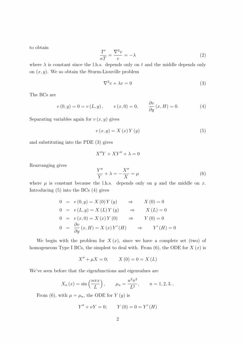
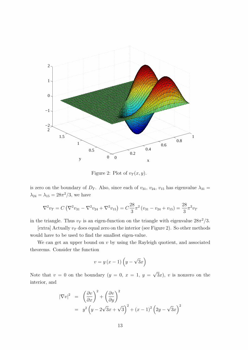
Figure 2: Plot of vT (x, y).

is zero on the boundary of DT . Also, since each of v31, v24, v15 has eigenvalue λ31 =

λ24 = λ15 = 28π2/3, we have

∇2vT = C�

∇2v31 −∇2v24 + ∇2v15

�

= C28

3π2 (v31 − v24 + v15) =

28

3π2vT

in the triangle. Thus vT is an eigen-function on the triangle with eigenvalue 28π2/3.

[extra] Actually vT does equal zero on the interior (see Figure 2). So other methods

would have to be used to find the smallest eigen-value.

We can get an upper bound on v by using the Rayleigh quotient, and associated

theorems. Consider the function

v = y (x − 1)�

y −√

3x�

Note that v = 0 on the boundary (y = 0, x = 1, y =√

3x), v is nonzero on the

interior, and

|∇v|2 =

�

∂v

∂x

�2

+

�

∂v

∂y

�2

= y2�

y − 2√

3x +√

3�2

+ (x − 1)2�

2y −√

3x�2

13

� � � �

�

The Rayleigh quotient is

� 1 � √3x � �2 2 � �22y y − 2√

3x + √

3 + (x − 1) 2y −√

3x dy dx 0 0

R (v) = � 1 �

� √3x �2 y2 (x − 1)2 � y −

√3x dy dx

0 0

1 √

3 112 15 = =3

≈ 37.3 1 √

3560

Thus by our theorem, the smallest eigenvalue on the triangle is less than 37.3. In

particular, the eigenvalue associated with vT was

28 λT = π2 ≈ 92.1

3

Clearly, this is NOT the smallest eigenvalue.

5 Problem 5

Consider the boundary value problem on the isosceles right angled triangle of side

length 1, 2 v = 0, 0 < y < x, 0 < x < 1∇

subject to the BCs

∂v (1, y) = 0, 0 < y < 1

∂x ∂v

(x, 0) = 0, 0 < x < 1 ∂y

v (x, x) = 0, 0 < x < 1/2

v (x, x) = 50, 1/2 < x < 1

Give a symmetry argument to show that v (x, 1 − x) = 25 for 0 < x < 1. Sketch the

level curves and heat flow lines of v. Be sure to sketch the region correctly before

solving the problem.

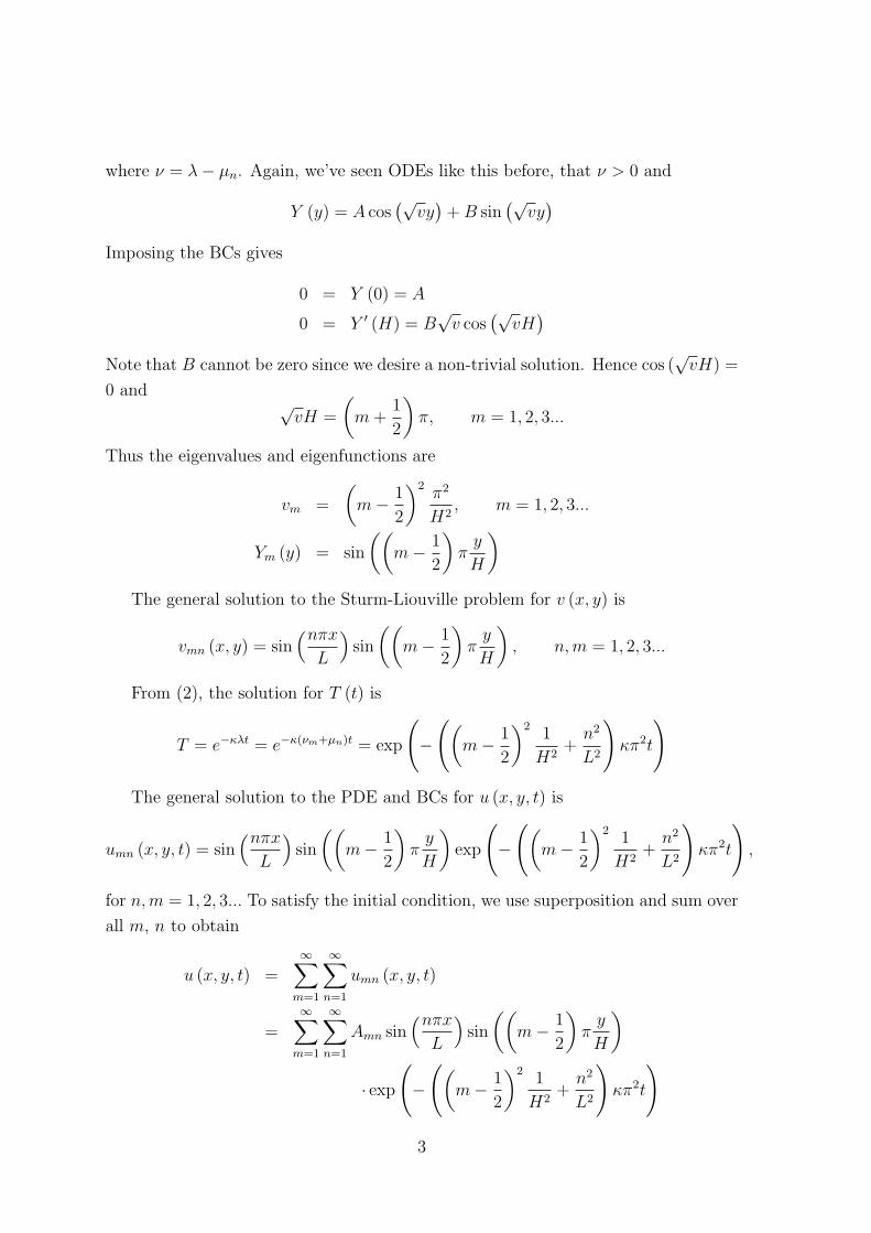
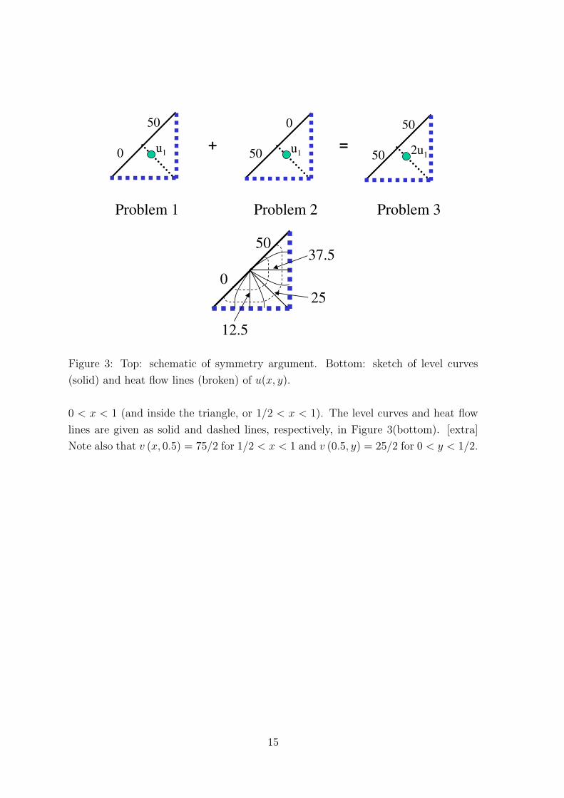
Solution: Take any point P = (x0, 1 − x0) on the line y = 1 − x inside the

triangle. Let v1 = v (x0, 1 − x0) be its steady-state temperature. Rotate the triangle

about the line y = 1−x. When you do this, the position of the point P doesn’t change

(see Figure 3(top) for a schematic of this argument). Add the solutions on the two

plates to obtain a triangular plate insulated on the horizontal and vertical side, and

kept at u = 50 on the hypotenuse. Thus the steady state temperature of this new

plate is 50. Hence v1 + v1 = 50, or v1 = 25. Since the point we chose was arbitrary,

then all points on the line y = 1 − x have steady state temp v (x, 1 − x) = 25 for

14

+ = 0

u1 u

1

0

1

50

50 50 2u

50

Problem 1 Problem 2 Problem 3

0

50

25

37.5

12.5

Figure 3: Top: schematic of symmetry argument. Bottom: sketch of level curves

(solid) and heat flow lines (broken) of u(x, y).

0 < x < 1 (and inside the triangle, or 1/2 < x < 1). The level curves and heat flow

lines are given as solid and dashed lines, respectively, in Figure 3(bottom). [extra]

Note also that v (x, 0.5) = 75/2 for 1/2 < x < 1 and v (0.5, y) = 25/2 for 0 < y < 1/2.

15