Embed Size (px)
Citation preview

The 2D Magnetohydrodynamic Equations
with Partial or Fractional Dissipation∗
Jiahong Wu†
Abstract
This paper surveys recent developments on the global regularity and related prob-lems on the 2D incompressible magnetohydrodynamic (MHD) equations with par-tial or fractional dissipation. The MHD equations with partial or fractional dissipa-tion are physically relevant and mathematically important. The global regularityand related problems have attracted considerable interests in recent years and therehave been substantial developments. In addition to reviewing the existing results,this paper also explains the difficulties associated with several open problems andsupply some new results.
c© Higher Education Pressand International PressBeijing-Boston
Lectures on the Analysis of NonlinearPartial Differential Equations Vol. 5MLM 5, pp. 283–332
1 Introduction
In the last few years there have been substantial developments on the global regu-larity problem concerning the magnetohydrodynamic (MHD) equations, especiallywhen there is only partial or fractional dissipation. This paper reviews some ofthese recent results and explains the difficulties associated with several open prob-lems in this direction. Attention will be focused on the two dimensional (2D)whole space case.
The MHD equations govern the motion of electrically conducting fluids suchas plasmas, liquid metals, and electrolytes. They consist of a coupled system ofthe Navier-Stokes equations of fluid dynamics and Maxwell’s equations of electro-magnetism. Since their initial derivation by the Nobel Laureate H. Alfven in 1924,the MHD equations have played pivotal roles in the study of many phenomena ingeophysics, astrophysics, cosmology and engineering (see, e.g., [4, 18]).
∗2010 Mathematics Subject Classification: 76W05, 76D03, 76B03, 35A05, 35Q35.Key words and phrases: Magnetohydrodynamic equations, partial dissipation, fractional
dissipation, global regularity†Department of Mathematics, Oklahoma State University, Stillwater, OK 74078. E-mail:
284 Jiahong Wu
The standard incompressible MHD equations can be written as⎧⎨⎩ut + u · ∇u = −∇p+ νΔu + b · ∇b,bt + u · ∇b = ηΔb+ b · ∇u,∇ · u = 0, ∇ · b = 0,
(1.1)
where u denotes the velocity field, b the magnetic field, p the pressure, ν ≥ 0 thekinematic viscosity and η ≥ 0 the magnetic diffusivity. Besides their wide phys-ical applicability, the MHD equations are also of great interest in mathematics.As a coupled system, the MHD equations contain much richer structures thanthe Navier-Stokes equations. They are not merely a combination of two paral-lel Navier-Stokes type equations but an interactive and integrated system. Theirdistinctive features make analytic studies a great challenge but offer new oppor-tunities.
Our attention will be focused on the initial-value problem of the MHD equa-tions with a given initial data (u0, b0) satisfying
u(x, 0) = u0(x), b(x, 0) = b0(x), ∇ · u0 = 0, ∇ · b0 = 0.
One of the fundamental problems concerning the MHD equations is whether phys-ically relevant regular solutions remain smooth for all time or they develop finitetime singularities. This problem can be extremely difficult, even in the 2D case.In recent years the MHD equations have attracted considerable interests and onefocus has been on the 2D MHD equations with partial or fractional dissipation.Important progress has been made.
We first explain why the study of the MHD equations with partial or frac-tional dissipation is relevant and important. When there is no kinematic dissi-pation or magnetic diffusion, the MHD equations become inviscid and the globalregularity problem appears to be out of reach at this moment. In contrast, whenboth the dissipation and the magnetic diffusion are present, the MHD equationsare fully dissipative and the global regularity problem in the 2D case can be solvedin a similar way as the one for the 2D Navier-Stokes equations. Mathematicallyit is natural to explore the intermediate equations that bridge the two extremes:the inviscid MHD and the fully dissipative MHD equations. The MHD equationswith partial or fractional dissipation exactly fill this gap. Physically, some ofthe partially dissipative MHD equations are important models in geophysical orastrophysical applications.
We elaborate on this point in more precise terms and summarize some of themain results on the 2D MHD equations with partial or fractional dissipation. Onestandard approach on the global regularity problem on the incompressible MHDequations is to divide the process into two steps. The first step is to show the localwell-posedness. This step is in general based on the contraction mapping principleand its variants such as successive approximations. In most circumstances weneed to restrict to small time interval in order to verify the conditions of thecontraction mapping principle. For many incompressible hydrodynamic modelssuch as the Navier-Stokes and the MHD equations, the local well-posedness canbe accomplished in this fashion when the initial data are sufficiently regular. The

Magnetohydrodynamic Equations 285
second step is to extend the local solution of the first step into a global (in time)one by establishing suitable global a priori bounds on the solutions. That is, oneneeds to prove that the solution remains bounded at any later time t, even thoughthe bound in general grows in time. Once we have the global bounds, the standardPicard type extension theorem allows us to extend the local solution into a globalone. Therefore, the global regularity problem on the MHD equations boils downto the global a priori bounds.
In the extreme case when the MHD equations are inviscid, namely⎧⎨⎩ut + u · ∇u = −∇p+ b · ∇b,bt + u · ∇b = b · ∇u,∇ · u = 0, ∇ · b = 0,
(1.2)
global bounds on (u, b) in any Sobolev space are not available. It is not clear ifsmooth solutions of (1.2) can blow up in a finite time, even though local well-posedness in sufficiently regular Sobolev or Besov type spaces are well-known. Wewill present in Section 2 this local well-posedness result and a regularity criterion.In addition, this section also provides two alternative formulations of the invis-cid MHD equations: the Lagrangian-Eulerian formulation and the formulation interms of a purely Lagrangian variable. These different formulations have their ownadvantages and may help understand the global regularity issue.
In another extreme case when the MHD equations are fully dissipative,namely ⎧⎨⎩ut + u · ∇u = −∇p+ νΔu + b · ∇b,
bt + u · ∇b = ηΔb+ b · ∇u,∇ · u = 0, ∇ · b = 0
(1.3)
with ν > 0 and η > 0, the global regularity problem can be solved similarly as forthe 2D Navier-Stokes equations. In fact, any initial data (u0, b0) ∈ L2(R2) with∇ · u0 = 0 and ∇ · b0 = 0 leads to a unique global solution (u, b) that becomesinfinitely smooth, namely (u, b) ∈ C∞(R2 × (t0,∞)) for any t0 > 0. This simpleglobal result is explained in Section 3.
Mathematically it is natural to examine intermediate equations that fill thegap between (1.2) and (1.3). One type of such equations are the MHD equationswith partial dissipation,⎧⎨⎩
ut + u · ∇u = −∇p+ ν1uxx + ν2uyy + b · ∇b,bt + u · ∇b = η1bxx + η2byy + b · ∇u,∇ · u = 0, ∇ · b = 0,
(1.4)
where the parameters ν1 ≥ 0, ν2 ≥ 0, η1 ≥ 0 and η2 ≥ 0. Clearly, when ν1 = ν2 =η1 = η2 = 0, (1.4) reduces to (1.2) while (1.4) with ν1 = ν2 > 0 and η1 = η2 > 0reduces to (1.3). Various partial dissipation cases arise when some of the fourparameters but not all are zero. Another type of intermediate equations thatbridge (1.2) and (1.3) are the 2D MHD equations with fractional dissipation⎧⎨⎩
ut + u · ∇u = −∇p− ν(−Δ)αu+ b · ∇b,bt + u · ∇b = −η(−Δ)βb+ b · ∇u,∇ · u = 0, ∇ · b = 0,
(1.5)

286 Jiahong Wu
where the fractional Laplacian operator is defined via the Fourier transform
(−Δ)αf(ξ) = |ξ|2αf(ξ).
When α = β = 1, (1.5) becomes (1.3) while α = β = 0, or more preciselyν = η = 0, corresponds to the inviscid MHD equations in (1.2). Recent efforts aredevoted to seeking the global regularity of (1.5) for smallest possible parametersα ≥ 0 and β ≥ 0.
One special partial dissipation case is the 2D resistive MHD equations, namely⎧⎨⎩ut + u · ∇u = −∇p+ b · ∇b,bt + u · ∇b = ηΔb+ b · ∇u,∇ · u = 0, ∇ · b = 0,
(1.6)
where η > 0 denotes the magnetic diffusivity (resistivity). (1.6) is applicable whenthe fluid viscosity can be ignored while the role of resistivity is important such asin magnetic reconnection and magnetic turbulence. Magnetic reconnection refersto the breaking and reconnecting of oppositely directed magnetic field lines in aplasma and is at the heart of many spectacular events in our solar system suchas solar flares and northern lights. The mathematical study of (1.6) may helpunderstand the Sweet-Parker model arising in magnetic reconnection theory [41].The global regularity problem is not completely solved at this moment, but recentefforts on this problem have significantly advanced our understanding. Global apriori bounds in very regular functional settings have been obtained, but the globalbound for ω ∈ L∞(0, T ;L∞) is lacking. As a consequence, the uniqueness and thehigher regularity can not be achieved. Section 4 reviews several recent results,explains the difficulty involved, details two hopeful attempts and discusses pathsthat may potentially yield the solution to this intriguing problem. In particular,we will present the work of Q. Jiu, D. Niu, J. Wu, X. Xu and H. Yu [30] as wellas some a priori estimates obtained in a work in progress with P. Zhang [54]. Inaddition, we state a theorem of C. Cao, J. Wu and B. Yuan [12] on a slightly moreregular system that points to the criticality of this global regularity problem.
Another significant partial dissipation case is the 2D MHD equations withvelocity dissipation and no resistivity, namely⎧⎨⎩ut + u · ∇u = −∇p+ νΔu + b · ∇b,
bt + u · ∇b = b · ∇u,∇ · u = 0, ∇ · b = 0,
(1.7)
(1.7) models fluids that can be treated as perfect conductors such as stronglycollisional plasmas. In addition, the breakdown of ideal MHD is known to bethe cause of solar flares, the largest explosions in the solar system [40]. Theintriguing problem of whether (1.7) can blow up in a finite time has recentlyattracted considerable interests. Recent strategy has been to seek global solutionsnear an equilibrium. Since the pioneering work of F. Lin, L. Xu and P. Zhang[36], this direction has flourished and a rich array of results have been obtained.Section 5 presents these recent results. We start with a local well-posedness resultof P. Constantin achieved via the Lagrangian-Eulerian approach. We then state
Magnetohydrodynamic Equations 287
and describe a global result (near an equilibrium) of Lin, Xu and Zhang [36] andtheir Lagrangian approach. We then present the main result of X. Ren, J. Wu, Z.Xiang and Z. Zhang [43] and outline the proof. A closely related work of J. Wu,Y. Wu and X. Xu [55] via the method of dispersive equations is then supplied. Wealso briefly summarize the results of X. Hu and F. Lin [27], and of T. Zhang [62].
Section 6 explains the global existence and uniqueness result of C. Cao and J.Wu [11] on the 2D MHD equations with mixed kinematic dissipation and magneticdiffusion, namely ⎧⎪⎨⎪⎩
ut + u · ∇u = −∇p+ νuyy + b · ∇b,bt + u · ∇b = ηbxx + b · ∇u,∇ · u = 0, ∇ · b = 0
or ⎧⎪⎨⎪⎩ut + u · ∇u = −∇p+ νuxx + b · ∇b,bt + u · ∇b = ηbyy + b · ∇u,∇ · u = 0, ∇ · b = 0.
Section 7 is devoted to the partial dissipation case when the 2D MHD equa-tions involve only the horizontal dissipation and the horizontal magnetic diffusion,⎧⎨⎩
∂tu+ u · ∇u = −∇p+ ∂xxu+ b · ∇b,∂tb + u · ∇b = ∂xxb+ b · ∇u,∇ · u = 0, ∇ · b = 0.
We describes the results of C. Cao, D. Regmi and J. Wu [8] as well as the resultsof a followup preprint of C. Cao, D. Regmi, J. Wu and X. Zheng [9].
The last section summarizes the results on the global regularity problemconcerning the incompressible MHD equations with fractional dissipation and pro-poses an open problem.
There is large literature on the MHD equations. This short survey focuseson the 2D incompressible MHD equations with partial or fractional dissipation.Due to the page constraints, we are not able to cover many significant results onthe MHD equations, especially those on the 3D MHD equations (see, e.g., [7, 10,14, 15, 16, 22, 23, 24, 25, 26, 29, 31, 33, 34, 37, 47, 49, 50, 52, 56, 58, 59, 61, 63]).
2 The inviscid MHD equations
This section is devoted to the initial-value problem for the inviscid MHD equations⎧⎪⎪⎨⎪⎪⎩ut + u · ∇u = −∇p+ b · ∇b,bt + u · ∇b = b · ∇u,∇ · u = 0, ∇ · b = 0,u(x, 0) = u0(x), b(x, 0) = b0(x)
(2.1)
where u0 and b0 satisfy ∇ · u0 = 0 and ∇ · b0 = 0. Whether or not a reasonablyregular initial datum (u0, b0) always leads to a globally regular solution of (2.1)

288 Jiahong Wu
remains an outstanding open problem. Besides the standard local existence anduniqueness result in the Sobolev setting, this section also provides two alternativeformulations of the inviscid MHD equations: a purely Lagrangian approach andthe Lagrangian-Eulerian formulation. These different formulations have their ownadvantages and may aid in the understanding of the global regularity issue. Therest of this section is divided into three subsections.
2.1 A standard local existence and uniqueness result
This subsection provides the local existence and uniqueness result in the Sobolevsetting and explains why it is difficult to prove global a priori bounds. The Beale-Kato-Majda type regularity criterion follows as a consequence of this explanation.
Theorem 2.1. Let s > 2. Assume (u0, b0) ∈ Hs(R2) with ∇ · u0 = 0 and∇ · b0 = 0. Then (2.1) has a unique local classical solution (u, b) ∈ C([0, T0);Hs)for some T0 = T0(‖(u0, b0)‖Hs) > 0. In addition, if, for T > T0,∫ T
0
(‖ω(t)‖B0∞,∞
+ ‖j(t)‖B0∞,∞
)dt <∞, (2.2)
then the solution remains in Hs for any t ≤ T . Here ω = ∇ × u denotes thevorticity and j = ∇× b denotes the current density.
Here B0∞,∞ denotes the homogeneous Besov space (see, e.g., [1, 2, 39, 44, 48]).The original Beale-Kato-Majda criterion on the 3D Euler equations involves theL∞-norm of the vorticity [38]. Due to the embedding
L∞ ↪→ B0∞,∞,
the assumption in (2.2) is weaker than the corresponding one with L∞-norm.The condition that (u0, b0) ∈ Hs(R2) with s > 2 may not be weakened to
(u0, b0) ∈ H2(R2). The work of Bourgain and Li [5, 6] on the Euler equations maybe extended to the inviscid MHD equations to indicate the ill-posedness of (2.1)in H2(R2).
The proof of the existence and uniqueness part in Theorem 2.1 is standard.One may follow the steps in the proof of Theorem 3.4 of the book by Majda andBertozzi [38], even though Theorem 3.4 there requires more regularity on the initialdata. Another approach is Friedrichs’ method, a regularization approximationprocess by spectral cutoffs (see, e.g., [1]). Our intention here is to explain why itis difficult to obtain global a priori bounds on the Sobolev norms of the solutions.The regularity criterion follows as a consequence.
Proof of Theorem 2.1. As we just remarked above, we only supply the proof forthe regularity criterion. In the process, we explain the difficulties associated withthe global bounds. When ∇ · b0 = 0, the solution (u, b) of (2.1) preserves thisproperty, namely ∇ · b = 0. This, together with ∇ · u = 0, allows us to obtain theL2-bound easily,
‖u(t)‖2L2 + ‖b(t)‖2
L2 = ‖u0‖2L2 + ‖b0‖2
L2 .
Magnetohydrodynamic Equations 289
But due to the lack of dissipation and magnetic diffusion, global bounds for anySobolev-norm appear to be impossible. We use the estimate of the H1-norm of(u, b) as an example. Due to ∇ · u = 0 and ∇ · b = 0,
‖∇u‖L2 = ‖ω‖L2 and ‖∇b‖L2 = ‖j‖L2,
and consequently it suffices to consider the L2-norm of (ω, j), which satisfies{ωt + u · ∇ω = b · ∇j,jt + u · ∇j = b · ∇ω + 2∂xb1(∂yu1 + ∂xu2) − 2∂xu1(∂yb1 + ∂xb2).
(2.3)
Dotting the first equation by ω and the second by j, adding up the resultingequations and integrating by parts, we have
12d
dt
(‖ω‖2L2 + ‖j‖2
L2
)= 2
∫j(∂xb1(∂yu1 + ∂xu2) − ∂xu1(∂yb1 + ∂xb2)).
We note that (2.3) does have a structure that allows us to eliminate four of thenonlinear terms. The terms on the right-hand side are of the triple product formand can not be bounded suitably unless we make the assumption∫ T
0
‖∇u‖∞dt <∞ or∫ T
0
‖j‖∞dt <∞.
This explains why we need (2.2) in order to control the H1-norm. More generallythe Hs-norm of (u, b) obeys the differential inequality, for Y (t) = ‖u(t)‖2
Hs +‖b(t)‖2
Hs ,d
dtY (t) ≤ C(‖∇u‖L∞ + ‖∇b‖L∞)Y (t). (2.4)
We can further bound ‖∇u‖L∞ and ‖∇b‖L∞ in terms of the logarithmic interpo-lation inequalities, for s > 2,
‖∇u‖L∞ ≤ C(1 + ‖u‖L2 + ‖ω‖B0∞,∞
log(1 + ‖u‖Hs)),
‖∇b‖L∞ ≤ C(1 + ‖b‖L2 + ‖j‖B0∞,∞
log(1 + ‖b‖Hs)).
Inserting the bounds above in (2.4) yields
d
dtY (t) ≤ C
(1 + ‖ω‖B0∞,∞
+ ‖j‖B0∞,∞
)Y (t) log(e+ Y (t)).
Osgood’s inequality then yields the desired regularity criterion part. This com-pletes the proof of Theorem 2.1.
2.2 Lagrangian-Eulerian type formulation
The Lagrangian-Eulerian approach of P. Constantin has the advantage that theLagrangian-Eulerian evolution system and the solution map are Lipschitz contin-uous in lower regularity path spaces and there is Lipschitz dependence of solutions
290 Jiahong Wu
on initial data in these spaces [17]. The inviscid MHD equations can not be writ-ten in the exact Lagrangian-Eulerian form of Constantin, but we can still recastthe inviscid MHD equations as an evolution system that shares some of the finecharacteristics of the original Lagrangian-Eulerian formulation.
We now detail this formulation and start with the particle trajectory. For asufficiently smooth velocity field u, say u ∈ L1(0, T ;W 1,∞), the particle trajectory(or flow map) X(a, t) with a ∈ R2 and t ≥ 0 obeys the ordinary differentialequation ⎧⎨⎩
dX(a, t)dt
= u(X(a, t), t),
X(a, 0) = a.
In addition, X(a, t) is invertible for any fixed t ∈ [0, T ], and we follow the notationof Constantin [17] to write the inverse as
X−1(x, t) = A(x, t),
which will also be called the “back-to-labels” map. The identities
A(X(a, t), t) = a for any a ∈ R2 and X(A(x, t), t) = x for any x ∈ R2
allow us to derive the equation of A,{∂tA+ u · ∇A = 0,A(x, 0) = x.
To derive the Lagrangian-Eulerian form, we rewrite the equation of b into anequivalent form. It is clear from the equation of b that
σ = b⊗ b ≡ (bibj)
satisfies∂tσ + u · ∇σ = (∇u)σ + σ(∇u)∗, (2.5)
where (∇u)∗ denotes the transpose of ∇u. Thus, we can write (2.1) as⎧⎨⎩∂tu+ u · ∇u = −∇p+ ∇ · σ,∇ · u = 0,∂tσ + u · ∇σ = (∇u)σ + σ(∇u)∗,
(2.6)
which, in terms of the vorticity ω and σ, can be further written as⎧⎨⎩∂tω + u · ∇ω = ∇×∇ · σ,u = ∇⊥Δ−1ω,∂tσ + u · ∇σ = (∇u)σ + σ(∇u)∗.
(2.7)
For notational convenience, we define the operators U and G as
u = U(ω) ≡ ∇⊥Δ−1ω, ∇u = G(ω) ≡ ∇∇⊥Δ−1ω.

Magnetohydrodynamic Equations 291
In terms of the Lagrangian variables
ζ(a, t) = ω ◦X ≡ ω(X(a, t), t) or ω(x, t) = ζ ◦A,τ(a, t) = σ ◦X or σ = τ ◦A,
(2.7) can be written as ⎧⎪⎨⎪⎩d
dtζ = (∇×∇ · (τ ◦A)) ◦X,
d
dtτ = gτ + τg∗,
(2.8)
whereg = G(ζ ◦A) ◦X.
Therefore, we have reduced the inviscid MHD equations in (2.1) to the followingsystem in terms of the Lagrangian variables X , ζ and τ as⎧⎪⎪⎪⎪⎪⎪⎨⎪⎪⎪⎪⎪⎪⎩
d
dtX = U(ζ ◦A) ◦X,
d
dtζ = (∇×∇ · (τ ◦A)) ◦X,
d
dtτ = gτ + τg∗.
Integrating in time yields⎧⎪⎪⎪⎪⎪⎪⎪⎨⎪⎪⎪⎪⎪⎪⎪⎩
X(a, t) = a+∫ t
0
U(ζ ◦A) ◦X(a, τ)dτ,
ζ(a, t) = ω0(a) +∫ t
0
(∇×∇ · (τ ◦A)) ◦X(a, τ)dτ,
τ(a, t) = (b0 ⊗ b0)(a) +∫ t
0
(gτ + τg∗)(τ)dτ.
We can summarize what we have derived above as the following theorem.
Theorem 2.2. The 2D inviscid incompressible MHD equations in (2.1) are for-mally equivalent to the following Lagrangian-Eulerian type formulation⎧⎪⎪⎪⎪⎪⎪⎪⎨⎪⎪⎪⎪⎪⎪⎪⎩
X(a, t) = a+∫ t
0
U(ζ ◦A) ◦X(a, τ)dτ,
ζ(a, t) = ω0(a) +∫ t
0
(∇×∇ · (τ ◦A)) ◦X(a, τ)dτ,
τ(a, t) = (b0 ⊗ b0)(a) +∫ t
0
(gτ + τg∗)(τ)dτ,
where X denotes the particle trajectory (or flow path), A is the inverse of X,ζ and τ are the Lagrangian counterparts of the Eulerian variables ω and b ⊗ b,respectively, and U(f) = ∇⊥Δ−1f corresponds to the 2D Biot-Savart kernel
U(f) =∫
R2K2(x− y)f(y)dy, K2(x) =
12π
x⊥
|x|2 , (2.9)

292 Jiahong Wu
G(f) ≡ ∇∇⊥Δ−1f is given by the explicit representation
G(f)(x, t) = PV∫
R2
P (x− y)|x− y|2 f(y)dy +
f(x)2
[0 −11 0
]with
P (z) =1
2π|z|2[
2z1z2 z22 − z2
1
z22 − z2
1 −2z1z2
],
and g = G(ζ ◦A) ◦X and g∗ is the transpose of g.
2.3 Purely Lagrangian formulation
It is possible to reformulate the inviscid MHD equations completely in terms of theparticle trajectory and the initial data. This purely Lagrangian formulation allowsus to represent all relevant physical quantities in terms of the particle trajectory.
Due to the divergence-free condition ∇ · b = 0, we can write b = ∇⊥ψ for ascalar function ψ and the induction equation for b,
∂tb + u · ∇b = b · ∇u, b(x, 0) = b0(x)
is then reduce to a transport equation for ψ,
∂tψ + u · ∇ψ = 0, ψ(x, 0) = ψ0(x)with ∇⊥ψ0 = b0. (2.10)
Equivalently, ψ can be represented by the back-to-labels map A (defined in theprevious subsection), namely the inverse of X ,
ψ(x, t) = ψ0(A(x, t)). (2.11)
Since b = ∇⊥ψ, we have j = ∇× b = Δψ and b · ∇j can be written in terms ofthe Poisson bracket
b · ∇j = J(ψ,Δψ),
where J is the usual Poisson bracket,
J(f, g) = ∂1f∂2g − ∂2f∂1g. (2.12)
Therefore, the vorticity equation
∂tω + u · ∇ω = b · ∇jcan be represented in the Lagrangian variable by
d
dt(ω ◦X) = J(ψ,Δψ) ◦X. (2.13)
J(ψ,Δψ) ◦X can be further represented in terms of ψ0 and X . In fact, accordingto (2.11) and the identity A(X(a, t), t) = a, we have
(∂1ψ) ◦X = J(ψ0, X2), (∂2ψ) ◦X = J(X1, ψ0),

Magnetohydrodynamic Equations 293
where J again is the Poisson bracket. ∂1Δψ and ∂2Δψ are more complex and weshall not presenting them. Integrating (2.13) in time yields
ω(X(a, t), t) = ω0(a) +∫ t
0
(J(ψ,Δψ) ◦X)(a, τ)dτ.
Therefore,
d
dtX(a, t)
= u(X(a, t), t)
=∫
R2K2(X(a, t) −X(a, t))ω(X(a, t), t)da
=∫
R2K2(X(a, t) −X(a, t))
(ω0(a) +
∫ t
0
(J(ψ,Δψ) ◦X)(a, τ)dτ)da
and X(a, 0) = a. We sum this up in the following theorem.
Theorem 2.3. The 2D inviscid incompressible MHD equations in (2.1) are for-mally equivalent to the following purely Lagrangian formulation
d
dtX(a, t) =
∫R2K2(X(a, t) −X(a, t))
·(ω0(a) +
∫ t
0
(J(ψ,Δψ) ◦X)(a, τ)dτ)da,
X(a, 0) = a,
where K2 is the Biot-Savart kernel defined in (2.9), J is the Poisson bracket definedin (2.12) and ∇⊥ψ = b.
3 The fully dissipative MHD equations
This section turns to another extreme case of the 2D incompressible MHD equa-tions, the fully dissipative MHD equations⎧⎪⎪⎨⎪⎪⎩
ut + u · ∇u = −∇p+ νΔu + b · ∇b,bt + u · ∇b = ηΔb+ b · ∇u,∇ · u = 0, ∇ · b = 0,u(x, 0) = u0(x), b(x, 0) = b0(x)
(3.1)
where u0 and b0 satisfy ∇ · u0 = 0 and ∇ · b0 = 0. The global regularity prob-lem on (3.1) can be solved following the similar approaches as those for the 2Dincompressible Navier-Stokes equations. The initial datum (u0, b0) does not haveto be smooth. In fact, any (u0, b0) ∈ L2(R2) leads to a unique global solution thatbecomes smooth instantaneously. More precisely, we have the following theorem.

294 Jiahong Wu
Theorem 3.1. Let (u0, b0) ∈ L2(R2). Then (3.1) has a unique global solution(u, b) satisfying,
u, b ∈ L∞(0,∞;L2(R2)) ∩ L2(0,∞; H1(R2)). (3.2)
In addition, for any t0 > 0, (u, b) is smooth,
(u, b) ∈ C∞(R2 × (t0,∞)). (3.3)
The approaches for the 2D incompressible Navier-Stokes equations can beextended to (3.1). One approach is to use the method of Friedriches, namelyregularization approximation via cutoffs in the Fourier space. The second approachis to use the classical fixed point theorem involving bilinear functions (see, e.g.,[1, p. 207]). We shall not provide the details here. In the following proof, weemphasize that solutions of the fully dissipative MHD equations in the naturalenergy space (3.2) are unique. In addition, we explain the mechanism why (3.3)is true.
Proof. As aforementioned, we only prove the uniqueness part and (3.3). Assumethat (u(1), b(1)) and (u(2), b(2)) are two solutions of (3.1). Then the difference
(u, b) = (u(1) − u(2), b(1) − b(2))
satisfies
∂tu+ u(1) · ∇u+ u · ∇u(2) = νΔu+ b(1) · ∇b+ b · ∇b(2),∂tb+ u(1) · ∇b + u · ∇b(2) = ηΔb+ b(1) · ∇u+ b · ∇u(2).
Taking the inner product with (u, b), we obtain after integration by parts,
12d
dt
(‖u‖2
L2 + ‖b‖2L2
)+ ν‖∇u‖2
L2 + η‖∇b‖2L2
= −∫u · ∇u(2) · u−
∫u · ∇b(2) · b
+∫b · ∇b(2) · u+
∫b · ∇u(2) · b. (3.4)
The four terms have similar structure and can be bounded similarly. We providethe bound for one of them. By Holder’s inequality and Sobolev’s inequality,∣∣∣∣∫ u · ∇b(2) · b
∣∣∣∣ ≤ ‖u‖L4‖b‖L4‖∇b(2)‖L2
≤ C‖∇b(2)‖L2‖u‖ 12L2‖∇u‖
12L2‖b‖
12L2‖∇b‖
12L2
≤ 18ν‖∇u‖2
L2 +18η‖∇b‖2
L2 + C‖∇b(2)‖2L2‖(u, b)‖2
L2.
After inserting these bounds in (3.4), we obtain
d
dt
(‖u‖2
L2 + ‖b‖2L2
)+ ν‖∇u‖2
L2 + η‖∇b‖2L2
≤ C(‖∇u(2)‖2
L2 + ‖∇b(2)‖2L2
)‖(u, b)‖2
L2.
Magnetohydrodynamic Equations 295
Applying Gronwall’s inequality and invoking the fact that u(2), b(2) ∈ L2(0,∞; H1)yield the desired uniqueness.
We now explain why (3.3) is true. Since (u, b) ∈ L2(0,∞; H1), then (u, b) isin H1 for almost every t ∈ (0,∞). For any t0 > 0, there is 0 < t1 < t0 such that(u(x, t1), b(x, t1)) ∈ H1(R2). Starting with (u(x, t1), b(x, t1)), we then solve (3.1).The solution (u, b) satisfies
(u, b) ∈ L∞(t1,∞;H1) ∩ L2(t1,∞; H2),
which allows us to further choose t2 ∈ (t1, t0) such that
(u(x, t2), b(x, t2)) ∈ H2(R2).
We then solve (3.1) with more regular initial datum and repeating the processleads to the desired smoothness. This completes the proof of Theorem 3.1.
4 The MHD equations with only magnetic diffu-sion
This section addresses the global regularity problem on the partial dissipation casewhen the 2D MHD equations involve only the magnetic diffusion,⎧⎪⎪⎨⎪⎪⎩
ut + u · ∇u = −∇p+ b · ∇b,bt + u · ∇b = ηΔb+ b · ∇u,∇ · u = 0, ∇ · b = 0,u(x, 0) = u0(x), b(x, 0) = b0(x),
(4.1)
where u0 and b0 satisfy ∇ · u0 = 0 and ∇ · b0 = 0. The global regularity prob-lem is not completely solved at this moment, but recent efforts have significantlyadvanced our understanding. Global a priori bounds in very regular functionalsettings have been obtained, for example, for any T > 0 and, for any p ∈ [2,∞)and q ∈ (1,∞),
(u, b) ∈ L∞(0,∞;H1), u ∈ Lq(0, T ;W 1,p), b ∈ Lq(0, T ;W 2,p),
ω ∈ L∞(0, T ;Lp), j ∈ L∞(0, T ;Lp)
where ω = ∇ × u is the vorticity and j = ∇ × b denotes the current density.Unfortunately the global bound for ω ∈ L∞(0, T ;L∞) is lacking. As a consequence,the uniqueness and the higher regularity can not be achieved. Various attemptshave been made to prove the global L∞ bound for ω. In particular, we will presentthe work of Q. Jiu, D. Niu, J. Wu, X. Xu and H. Yu [30] and some a priori estimatesobtained in a work in progress with P. Zhang [54]. In addition, several combinedquantities have been discovered to be globally bounded in highly regular functionalsettings.
This section reviews several recent results, explains the difficulty involved,describes some of the attempts and discusses paths that may potentially lead tothe solution to this intriguing problem. We divide the rest of this section into foursubsections.
296 Jiahong Wu
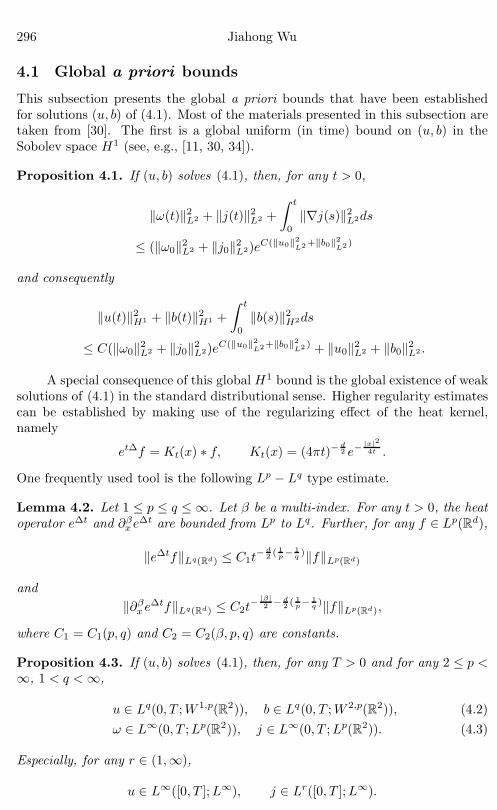
4.1 Global a priori bounds
This subsection presents the global a priori bounds that have been establishedfor solutions (u, b) of (4.1). Most of the materials presented in this subsection aretaken from [30]. The first is a global uniform (in time) bound on (u, b) in theSobolev space H1 (see, e.g., [11, 30, 34]).
Proposition 4.1. If (u, b) solves (4.1), then, for any t > 0,
‖ω(t)‖2L2 + ‖j(t)‖2
L2 +∫ t
0
‖∇j(s)‖2L2ds
≤ (‖ω0‖2L2 + ‖j0‖2
L2)eC(‖u0‖2L2+‖b0‖2
L2)
and consequently
‖u(t)‖2H1 + ‖b(t)‖2
H1 +∫ t
0
‖b(s)‖2H2ds
≤ C(‖ω0‖2L2 + ‖j0‖2
L2)eC(‖u0‖2L2+‖b0‖2
L2 ) + ‖u0‖2L2 + ‖b0‖2
L2 .
A special consequence of this global H1 bound is the global existence of weaksolutions of (4.1) in the standard distributional sense. Higher regularity estimatescan be established by making use of the regularizing effect of the heat kernel,namely
etΔf = Kt(x) ∗ f, Kt(x) = (4πt)−d2 e−
|x|24t .
One frequently used tool is the following Lp − Lq type estimate.
Lemma 4.2. Let 1 ≤ p ≤ q ≤ ∞. Let β be a multi-index. For any t > 0, the heatoperator eΔt and ∂β
x eΔt are bounded from Lp to Lq. Further, for any f ∈ Lp(Rd),
‖eΔtf‖Lq(Rd) ≤ C1t− d
2 ( 1p− 1
q )‖f‖Lp(Rd)
and‖∂β
xeΔtf‖Lq(Rd) ≤ C2t
− |β|2 − d
2 ( 1p− 1
q )‖f‖Lp(Rd),
where C1 = C1(p, q) and C2 = C2(β, p, q) are constants.
Proposition 4.3. If (u, b) solves (4.1), then, for any T > 0 and for any 2 ≤ p <∞, 1 < q <∞,
u ∈ Lq(0, T ;W 1,p(R2)), b ∈ Lq(0, T ;W 2,p(R2)), (4.2)ω ∈ L∞(0, T ;Lp(R2)), j ∈ L∞(0, T ;Lp(R2)). (4.3)
Especially, for any r ∈ (1,∞),
u ∈ L∞([0, T ];L∞), j ∈ Lr([0, T ];L∞).

Magnetohydrodynamic Equations 297
Proof. The proof makes use of the maximal LqtL
px regularity for the heat kernel
(see, e.g., [35]). That is, the operator A defined by
Af ≡∫ t
0
e(t−s)ΔΔf(s)ds
is bounded from Lp(0, T ;Lq(Rd)) to Lp(0, T ;Lq(Rd)) for every fixed T ∈ (0,∞].Resorting to the heat kernel, we write the equation of b in the integral form
b(x, t) = etΔb0 +∫ t
0
e(t−s)Δ∇ · f(s, ·)ds, (4.4)
with f = (fi) and fi = biu − uib (i = 1, 2). The global bound in Proposition 4.1and Sobolev’s inequality imply that, for any p ∈ [2,∞),
fi ∈ L∞(0, T ;Lp).
(4.4), combined with Lemma 4.2, leads to a global L∞ bound for b,
‖b‖L∞(0,T ;L∞)
≤ C(‖Kt‖L∞(0,T ;L1)‖b0‖L∞ + ‖∇Kt‖L1(0,T ;Lp′)‖f‖L∞(0,T ;Lp))
≤ C(‖b0‖L∞ + ‖u‖L∞(0,T ;H1)‖b‖L∞(0,T ;H1)).
(4.4), together with the maximal LqtL
px regularity, yields
‖∇b‖Lq(0,T ;Lp) ≤C(‖Kt‖Lq(0,T ;L1)‖∇b0‖Lp + ‖f‖Lq(0,T ;Lp))≤C(‖b0‖H2 + ‖u‖L∞(0,T ;H1)‖b‖L∞(0,T ;H1)).
The global bounds for ‖Δb‖Lq(0,T ;Lp) and ‖ω‖Lq(0,T ;Lp) are obtained simultane-ously,
‖ω(t)‖Lp ≤ C(‖ω0‖Lp + ‖Δb‖Lqt Lp),
‖Δb‖Lqt Lp ≤ C(‖Δb0‖Lp + ‖b‖L∞
t L∞‖ω‖LqtLp + ‖u‖L2
tH1‖∇b‖L
2q2−qt L2p
).
The two estimates above and Gronwall’s inequality yield the desired bounds in(4.3). The global bound for j ∈ L∞(0, T ;Lp) in (4.3) follows from energy estimatesinvolving the equation of j and the global bound for ω ∈ L∞(0, T ;Lp) follows fromenergy estimates on the vorticity equation. This completes the proof of Proposition4.3.
4.2 An attempt to bound ‖ω‖L∞(0,T ;L∞) and an equation fora combined quantity G = ω + curl∇ · (b ⊗ b)
It appears that the global a priori bounds in the previous subsection are notsufficient to hammer out the problem. The missing piece in the puzzle is a globalbound for ‖ω‖L∞(0,T ;L∞). Various attempts have been made to establish this

298 Jiahong Wu
global bound. This subsection provides two of them. The first one is to work witha combined quantity while the second one is a work in progress with P. Zhang [54].
In the paper of Q. Jiu, D. Niu, J. Wu, X. Xu and H. Yu [30], we attemptedto solve the global regularity problem by working with a combined quantity. Weare close to solving this problem and [30] provides a regularity criterion.
Theorem 4.4. Let s > 2. Assume (u0, b0) ∈ Hs(R2) with ∇ · u0 = ∇ · b0 = 0.Let (u, b) be the local (in time) solution of (1.1) on [0, T ∗). Let T0 > T ∗. If thereis σ > 0 and an integer k0 > 0 such that b satisfies
M(T0) ≡∫ T0
0
∑k≥k0
2σk‖Sk−1(b⊗ b)‖L∞dt <∞, (4.5)
then the local solution can be extended to [0, T0]. Here b ⊗ b denotes the tensorproduct and Sj denotes the identity approximator defined via the Littlewood-Paleydecomposition.
We explain the proof of Theorem 4.4. Due to the lack of a global bound on∇j in L∞, the vorticity equation
∂tω + u · ∇ω = b · ∇j (4.6)
does not allow us to extract a global bound for ‖ω‖L∞. A natural idea is toeliminate this bad term. To this end, we rewrite the vorticity equation as
∂tω + u · ∇ω = curl∇ · (b⊗ b) (4.7)
and recast the equation of b as
(b⊗ b)t + u · ∇(b ⊗ b) = ∇u(b⊗ b) + (b ⊗ b)(∇u)∗
+Δ(b⊗ b) − 22∑
k=1
(∂kb⊗ ∂kb). (4.8)
Applying R ≡ (−Δ)−1curl∇· to (4.8) yields to((R(b ⊗ b)
)t+u · ∇R(b⊗ b)
= −[R, u · ∇](b⊗ b) + R(∇u(b⊗ b) + (b ⊗ b)(∇u)∗)
−curl∇ · (b⊗ b) − 22∑
k=1
R(∂kb⊗ ∂kb). (4.9)
Adding (4.9) to (4.7) and setting G = ω + R(b ⊗ b), we get
∂tG+ u · ∇G = −[R, u · ∇](b ⊗ b) − 22∑
k=1
R(∂kb⊗ ∂kb)
+R(∇u(b⊗ b)) + R((b ⊗ b)(∇u)∗). (4.10)
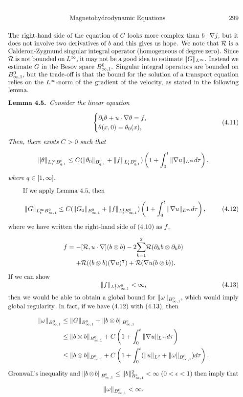
Magnetohydrodynamic Equations 299
The right-hand side of the equation of G looks more complex than b · ∇j, but itdoes not involve two derivatives of b and this gives us hope. We note that R is aCalderon-Zygmund singular integral operator (homogeneous of degree zero). SinceR is not bounded on L∞, it may not be a good idea to estimate ‖G‖L∞ . Instead weestimate G in the Besov space B0∞,1. Singular integral operators are bounded onB0
∞,1, but the trade-off is that the bound for the solution of a transport equationrelies on the L∞-norm of the gradient of the velocity, as stated in the followinglemma.
Lemma 4.5. Consider the linear equation{∂tθ + u · ∇θ = f,
θ(x, 0) = θ0(x),(4.11)
Then, there exists C > 0 such that
‖θ‖L∞t B0
q,1≤ C(‖θ0‖B0
q,1+ ‖f‖L1
tB0q,1
)(
1 +∫ t
0
‖∇u‖L∞dτ
),
where q ∈ [1,∞].
If we apply Lemma 4.5, then
‖G‖L∞t B0
∞,1≤ C(‖G0‖B0
∞,1+ ‖f‖L1
tB0∞,1
)(
1 +∫ t
0
‖∇u‖L∞dτ
), (4.12)
where we have written the right-hand side of (4.10) as f ,
f = −[R, u · ∇](b⊗ b) − 22∑
k=1
R(∂kb⊗ ∂kb)
+R((b ⊗ b)(∇u)ᵀ) + R(∇u(b⊗ b)).
If we can show‖f‖L1
tB0∞,1
<∞, (4.13)
then we would be able to obtain a global bound for ‖ω‖B0∞,1
, which would implyglobal regularity. In fact, if we have (4.12) with (4.13), then
‖ω‖B0∞,1
≤ ‖G‖B0∞,1
+ ‖b⊗ b‖B0∞,1
≤ ‖b⊗ b‖B0∞,1
+ C
(1 +
∫ t
0
‖∇u‖L∞dτ
)≤ ‖b⊗ b‖B0
∞,1+ C
(1 +
∫ t
0
(‖u‖L2 + ‖ω‖B0∞,1
)dτ).
Gronwall’s inequality and ‖b⊗ b‖B0∞,1
≤ ‖b‖2Bε
∞,1<∞ (0 < ε < 1) then imply that
‖ω‖B0∞,1
<∞.

300 Jiahong Wu
Especially, ‖ω‖L∞ <∞. Then higher regularities follow.It then remains to check (4.13). f involves a commutator and the following
lemma provides a bound of such a commutator in Besov spaces. This type ofestimates can be found in [28, 45].
Lemma 4.6. Let R denote a standard singular integral operator, say Riesz trans-form or R = (−Δ)−1curl∇·. Let 1 < p ≤ ∞. For any integer k, for 0 ≤ s1, s2 ≤ 1and s1 + s2 ≤ 1, we have
‖Δk([R, u · ∇]θ)‖Lp ≤ Cs2(1−s1−s2)k‖Λs1u‖Lp1‖Λs2θ‖Lp2 (4.14)
where 1 < p1, p2 ≤ ∞ and 1p = 1
p1+ 1
p2.
The global a priori bounds obtained in the previous subsection allow us tobound the first two terms in f without any problem. The last two terms in f aresimilar and each one of them is split into three parts by the notion of paraproducts.It is only one of these parts that need the assumption in (4.5) to be bounded. Hereare more details. By Lemma 4.6, for s ∈ (0, 1),
‖[R, u · ∇](b ⊗ b)‖B0∞,1
≤ C‖Λsu‖B0∞,1
‖Λ1−s(b ⊗ b)‖B0∞,1
.
For any s ∈ (0, 1), ‖Λsu‖B0∞,1
can be bounded by ‖ω‖Lq for some large q ∈ (2,∞).In fact, by Bernstein’s inequality,
‖Λsu‖B0∞,1
≤ ‖Δ−1Λsu‖L∞ +∞∑
k=0
‖ΔkΛsu‖L∞
≤ C‖u‖L2 + C
∞∑k=0
2(s−1)k‖Δkω‖L∞
≤ C‖u‖L2 + C∞∑
k=0
2(s−1+ 2q )k‖Δkω‖Lq
≤ C‖u‖L2 + C‖ω‖Lq
∞∑k=0
2(s−1+ 2q )k.
Therefore, if we choose q ∈ (2,∞) such that s− 1 + 2q < 0, then
‖Λsu‖B0∞,1
≤ C(‖u‖L2 + ‖ω‖Lq) <∞.
The regularity of b also implies that, for s ∈ (0, 1) close to 1,
‖Λ1−s(b ⊗ b)‖B0∞,1
<∞.
In fact, in a similar fashion as above, if q ∈ (2,∞) such that −s+ ε+ 2eq < 0,
‖Λ1−s(b ⊗ b)‖B0∞,1
≤C‖Λ1−sb‖2Bε
∞,1≤ C(‖b‖2
L2 + ‖∇b‖2Leq).

Magnetohydrodynamic Equations 301
Therefore, Proposition 4.3 implies
‖[R, u · ∇](b ⊗ b)‖L1tB0
∞,1
≤ C(‖u‖L∞t L2 + ‖ω‖L∞
t Lq)(‖b‖2L2
tL2 + ‖∇b‖2L2
tLeq) <∞.
We now estimate the second term in f . For any ε > 0,∥∥∥∥∥2∑
k=1
R(∂kb⊗ ∂kb)
∥∥∥∥∥B0
∞,1
≤ ‖∇b‖2Bε
∞,1.
By Bernstein’s inequality,
‖∇b‖Bε∞,1
≤ C‖b‖L2 + C
∞∑k=0
2εk‖Δk∇b‖L∞
≤ C‖b‖L2 + C
∞∑k=0
2k(ε+1+ 2q )‖Δkb‖Lq
≤ C‖b‖L2 + C
∞∑k=0
2k(ε+1+ 2q −γ)‖ΛγΔkb‖Lq
≤ C‖b‖L2 + C‖Λγb‖Lq ,
where ε+ 1 + 2q < γ < 2. Therefore,∥∥∥∥∥
2∑k=1
R(∂kb⊗ ∂kb)
∥∥∥∥∥L1
t B0∞,1
≤ ‖∇b‖2L2
tBε∞,1
≤ C‖b‖2L2
tL2 + C‖Λγb‖2L2
t Lq <∞.
We bound the last two terms in f . Their estimates are similar and we shall handleone of them. By Bernstein’s inequality,
‖R(∇u(b⊗ b))‖B0∞,1
≤C‖Δ−1(∇u(b⊗ b))‖L2 +∞∑
k=0
‖Δk(∇u(b ⊗ b))‖L∞
≤C‖ω‖L2‖b‖2L∞ +
∞∑k=0
‖Δk(∇u(b ⊗ b))‖L∞ .
Following the notion of paraproducts, we write
Δk(∇u(b⊗ b)) =∑
|k−m|≤2
Δk(Sm−1∇uΔm(b⊗ b))
+∑
|k−m|≤2
Δk(Δm∇uSm−1(b⊗ b))
+∑
m≥k−1
Δk(Δm∇uΔm(b⊗ b)), (4.15)

302 Jiahong Wu
where Δm = Δm+1 + Δm + Δm−1. By Bernstein’s inequality,∑|k−m|≤2
‖Δk(Sm−1∇uΔm(b ⊗ b))‖L∞
≤∑
|k−m|≤2
‖Sm−1∇u‖L∞‖Δm(b⊗ b)‖L∞
≤ C∑
|k−m|≤2
22q m‖Sm−1ω‖Lq‖Δm(b ⊗ b)‖L∞
≤ C‖ω‖Lq
∑|k−m|≤2
22q m‖Δm(b ⊗ b)‖L∞.
By Bernstein’s inequality and the Hardy-Littlewood-Sobolev inequality, the thirdterm in (4.15) can be bounded by∑
m≥k−1
‖Δk(Δm∇uΔm(b⊗ b))‖L∞
=∑
m≥k−1
‖ΔkΛ2q Λ− 2
q (Δm∇uΔm(b ⊗ b))‖L∞
≤∑
m≥k−1
22q k‖Λ− 2
q (Δm∇uΔm(b⊗ b))‖L∞
≤ C∑
m≥k−1
22q k‖Δm∇u‖Lq‖Δm(b⊗ b)‖L∞
≤ C‖ω‖Lq
∑m≥k−1
22q (k−m)2
2q m‖Δm(b ⊗ b)‖L∞ .
The condition (4.5) is needed to handle the second term in (4.15). As in theestimate of the first term, we have∑
|k−m|≤2
‖Δk(Δm∇uSm−1(b⊗ b))‖L∞
≤ C‖ω‖Lq
∑|k−m|≤2
22q m‖Sm−1(b⊗ b)‖L∞ .
Combining the estimates above, we have
‖R(∇u(b⊗ b))‖B0∞,1
≤ C‖ω‖L2‖b‖2L∞ + C‖ω‖Lq
∑k≥0
∑|k−m|≤2
22q m‖Δm(b ⊗ b)‖L∞
+C‖ω‖Lq
∑k≥0
∑m≥k−1
22q (k−m)2
2q m‖Δm(b⊗ b)‖L∞
+C‖ω‖Lq
∑k≥0
∑|k−m|≤2
22q m‖Sm−1(b⊗ b)‖L∞

Magnetohydrodynamic Equations 303
≤ C‖ω‖L2‖b‖2L∞ + C‖ω‖Lq‖b‖L∞‖b‖
B2q∞,1
+C‖ω‖Lq
∑k≥0
22q k‖Sk−1(b⊗ b)‖L∞ . (4.16)
We provide some details for the last inequality, namely∑k≥0
∑|k−m|≤2
22q m‖Δm(b ⊗ b)‖L∞ ≤ C‖b‖L∞‖b‖
B2q∞,1
, (4.17)
∑k≥0
∑m≥k−1
22q (k−m)2
2q m‖Δm(b⊗ b)‖L∞ ≤ C‖b‖L∞‖b‖
B2q∞,1
. (4.18)
In fact, by the paraproduct decomposition,∑k≥0
∑|k−m|≤2
22q m‖Δm(b⊗ b)‖L∞
≤ C∑k≥0
22q k
∑|k−l|≤2
‖Δk(Sl−1b⊗ Δlb)‖L∞
+C∑k≥0
22q k
∑|k−l|≤2
‖Δk(Δlb⊗ Sl−1b)‖L∞
+C∑k≥0
22q k
∑l≥k−1
‖Δk(Δlb⊗ Δlb)‖L∞
≤ C∑k≥0
22q k‖b‖L∞‖Δkb‖L∞
+C∑k≥0
∑l≥k−1
22q (k−l)‖b‖L∞2
2q l‖Δlb‖L∞
≤ C‖b‖L∞‖b‖B
2q∞,1
.
This proves (4.17). The proof of (4.18) is similar. Due to (4.5), the third term istime integrable if we choose q large enough, say 2
q < σ. Therefore we have proven(4.13). This completes the proof of Theorem 4.4.
4.3 Another attempt to bound ‖ω‖L∞(0,T ;L∞)
This subsection describes an attempt to bound ‖ω‖L∞(0,T ;L∞) via a more directapproach. This is part of the work in progress with P. Zhang [54]. It follows fromthe vorticity equation (4.6) that
‖ω(t)‖L∞ ≤ ‖ω0‖L∞ + C‖b‖L∞t,x‖∇j‖L1
t L∞x. (4.19)
We know that ‖b‖L∞t,x
is bounded according to the a priori bounds of the previoussubsection. A natural idea would be to bound ‖∇j‖L1
tL∞x
directly. We obtain thefollowing proposition.

304 Jiahong Wu
Proposition 4.7. Assume that (u, b) is classical solution of (4.1). Then,
‖∇j‖L1tB0
∞,1≤ ‖j0‖B−1
∞,1+ C‖ω‖L1
tB0∞,1
+ C,
where C depends on the initial data and t only.
We remark that, if we could bound ‖∇j‖L1tL∞
xin terms of ‖ω‖L1
tL∞x
, theglobal regularity problem would be solved. In fact, it follows from (4.19) that
‖ω(t)‖L∞ ≤ ‖ω0‖L∞ + C‖b‖L∞t,x‖∇j‖L1
tB0∞,1
≤ ‖ω0‖L∞ + C‖b‖L∞t,x‖ω‖L1
tL∞ .
Gronwall’s inequality then yields the global bound on ‖ω(t)‖L∞ . As we shall seein the proof of Proposition 4.7, it is just one paraproduct part of one term thatprevents us from bounding ‖∇j‖L1
tL∞x
in terms of ‖ω‖L1tL∞
x.
In order to prove Proposition 4.7, we need a simple fact on the smoothingeffort of the heat operator eΔt on distributions with Fourier transform supportedon annulus (see, e.g., [1]).
Lemma 4.8. There exist two constants C1 > 0 and C2 > 0 such that, for anyq ∈ [1,∞],
‖eνΔΔkf‖Lq(Rd) ≤ C1e−C2ν22j‖Δkf‖Lq(Rd),
where ν > 0 is a parameter and Δk denotes the homogeneous Littlewood-Paleyblocks.
We can now prove Proposition 4.7.
Proof of Proposition 4.7. We know that j = ∇× b satisfies
∂tj + u · ∇j = Δj + b · ∇ω +Q,
where
Q = 2∂1b1(∂2u1 + ∂1u2) − 2∂1u1(∂2b1 + ∂1b2). (4.20)
The corresponding integral form is given by
j(t) = etΔj0 −∫ t
0
e(t−τ)Δ(u · ∇j)(τ)dτ
+∫ t
0
e(t−τ)Δ(b · ∇ω)(τ)dτ +∫ t
0
e(t−τ)ΔQ(τ)dτ. (4.21)
Applying Δk to (4.21) yields
Δkj(t) = etΔΔkj0 −∫ t
0
e(t−τ)ΔΔk(u · ∇j)(τ)dτ
+∫ t
0
e(t−τ)ΔΔk(b · ∇ω)(τ)dτ +∫ t
0
e(t−τ)ΔΔkQ(τ)dτ.

Magnetohydrodynamic Equations 305
According to Lemma 4.8, we have
‖Δkj(t)‖L∞ ≤ Ce−C22kt‖Δkj0‖L∞ + J1 + J2 + J3, (4.22)
where
J1 =∥∥∥∥∫ t
0
e(t−τ)ΔΔk(u · ∇j)(τ)dτ∥∥∥∥
L∞
≤ C
∫ t
0
e−C(t−τ)22k‖Δk(u · ∇j)(τ)‖L∞dτ,
J2 =∥∥∥∥∫ t
0
e(t−τ)ΔΔk(b · ∇ω)(τ)dτ∥∥∥∥
L∞
≤ C
∫ t
0
e−C(t−τ)22k‖Δk(b · ∇ω)(τ)‖L∞dτ,
J3 =∥∥∥∥∫ t
0
e(t−τ)ΔΔkQ(τ)dτ∥∥∥∥
L∞
≤ C
∫ t
0
e−C(t−τ)22k‖ΔkQ(τ)‖L∞dτ.
To estimate J1, we invoke the notion of paraproduct to write
Δk(u · ∇j) =∑
|j−k|≤2
Δk(Sl−1u · ∇Δlj)
+∑
|j−k|≤2
Δk(Δlu · ∇Sl−1j) +∑
l≥k−1
Δk(Δlu · ∇Δlj).
Employing the bound on u in Proposition 4.3, we have
‖Δk(u · ∇j)‖L∞ ≤ C2k‖u‖L∞‖Δkj‖L∞ + C‖u‖L∞∑
m≤k−1
2m‖Δmj‖L∞
+C‖u‖L∞2k∑
l≥k−1
‖Δlj‖L∞ .
Therefore,
J1 ≤ C‖u‖L∞
[ ∫ t
0
e−C(t−τ)22k(2k‖Δkj‖L∞ +
∑m≤k−1
2m‖Δmj‖L∞
+2k∑
l≥k−1
‖Δlj‖L∞)dτ
]. (4.23)
We now turn to J2. To estimate J2, we write
Δk(b · ∇ω) =∑
|l−k|≤2
Δk(Sl−1b · Δl∇ω) +∑
|l−k|≤2
Δk(Δlb · Sl−1∇ω)
+∑
l≥k−1
Δk(Δlb · Δl∇ω).

306 Jiahong Wu
Thus,
‖Δk(b · ∇ω)‖L∞ ≤ C2k‖Sk−1b‖L∞‖Δkω‖L∞ + C2k‖Δkb‖L∞‖ω‖L∞
+∑
l≥k−1
2k‖Δlb‖L∞‖ω‖L∞.
Therefore,
J2 ≤ C
∫ t
0
e−C(t−τ)22k(2k‖Sk−1b‖L∞‖Δkω‖L∞ + 2k‖Δkb‖L∞‖ω‖L∞
+∑
l≥k−1
2k‖Δlb‖L∞‖ω‖L∞)dτ. (4.24)
The difficult term is C2k‖Sk−1b‖L∞‖Δkω‖L∞. The other terms are all right. Wenow turn to J3. Recalling the definition of Q in (4.20), it suffices to deal with thetypical term
∂1b1∂2u1.
To estimate ∂1b1∂2u1, we write Δk(∂1b1∂2u1) into paraproducts
Δk(∂1b1∂2u1) =∑
|l−k|≤2
Δk(Sl−1∂1b1Δl∂2u1)
+∑
|l−k|≤2
Δk(Δl∂1b1Sl−1∂2u1)
+∑
l≥k−1
Δk(Δl∂1b1Δl∂2u1).
By Bernstein’s inequality,
‖Δk(∂1b1∂2u1)‖L∞ ≤ C‖Sk−1∂1b1‖L∞‖Δk∂2u1‖L∞
+C‖Sk−1∂2u1‖L∞‖Δk∂1b1‖L∞
+C∑
l≥k−1
‖Δl∂1b1‖L∞‖Δl∂2u1‖L∞
≤ C2k‖∇b‖L∞‖Δku‖L∞
+C2k‖u‖L∞‖Δk∇b‖L∞
+C‖u‖L∞∑
l≥k−1
2k−l‖ΔΔlb‖L∞ .
Now we then multiply (4.22) by 2k and integrate in time to obtain
2k‖Δkj‖L1t L∞ ≤ 2−k‖Δkj0‖L∞ + 2k‖J1‖L1
t+ 2k‖J2‖L1
t+ 2k‖J3‖L1
t. (4.25)
Invoking the bound in (4.23) and applying Young’s inequality for convolution yield
2k‖J1‖L1t≤ C2−k‖u‖L∞2k‖Δkj‖L1
tL∞
+C2−k‖u‖L∞∑
m≤k−1
2m‖Δmj‖L1tL∞
+C2−k‖u‖L∞∑
l≥k−1
2k−l2l‖Δlj‖L1tL∞ .

Magnetohydrodynamic Equations 307
Similarly,
2k‖J2‖L1t≤ C‖b‖L∞
t,x‖Δkω‖L1
tL∞
+C‖ω‖L1tL∞
x‖Δkb‖L∞
t,x+ C‖ω‖L1
tL∞x
∑l≥k−1
‖Δlb‖L∞t,x
and
2k‖J3‖L1t≤ C‖Δku‖L∞
t L∞x‖∇b‖L1
tL∞x
+C‖u‖L∞t L∞
x‖Δk∇b‖L1
t L∞x
+C2−k‖u‖L∞t L∞
x
∑l≥k−1
2k−l‖ΔΔlb‖L∞.
We choose N > 0 sufficiently large such that
2−N‖u‖L∞ <116.
Summing over k ≥ N in (4.25) and invoking the global bounds in Proposition 4.3,we have
∞∑k=N
2k‖Δkj‖L1t L∞ ≤
∞∑k=N
2−k‖Δkj0‖L∞ +14
∞∑k=0
2k‖Δkj‖L1tL∞
+C∞∑
k=N
‖Δkω‖L1tL∞ + C(1 + ‖ω‖L1
tL∞). (4.26)
In addition, by Proposition 4.3,
N−1∑k=0
2k‖Δkj‖L1t L∞ <∞.
Inserting this bound in (4.26) yields
‖j‖L1tB1
∞,1≤ ‖j0‖B−1
∞,1+
14‖j‖L1
tB1∞,1
+N−1∑k=0
2k‖Δkj‖L1tL∞ + C‖ω‖L1
tB0∞,1
+ C(1 + ‖ω‖L1tL∞).
We thus have obtained that
‖∇j‖L1tB0
∞,1≤ ‖j0‖B−1
∞,1+ C‖ω‖L1
tB0∞,1
+ C.
This completes the proof of Proposition 4.7.

308 Jiahong Wu
4.4 The criticality
The global regularity problem on the 2D MHD equations with only magneticdiffusion (4.1) is critical in two senses. The first is that solutions of (4.1) admitglobal bounds in very regular functional settings such as
‖ω‖L∞(0,T ;Lp) for any 1 < p <∞,
but the crucial global bound on ‖ω‖L∞(0,T ;L∞) is missing. The second is that, ifwe replace Δb by (−Δ)βb with any β > 1, the resulting system then admits aunique global solution. More precisely, we have the following theorem.
Theorem 4.9. Consider the following 2D MHD equations with fractional mag-netic diffusion⎧⎪⎪⎪⎨⎪⎪⎪⎩
∂tu+ u · ∇u = −∇p+ b · ∇b, x ∈ R2, t > 0,∂tb+ u · ∇b+ (−Δ)βb = b · ∇u, x ∈ R2, t > 0,∇ · u = 0, ∇ · b = 0, x ∈ R2, t > 0,u(x, 0) = u0(x), b(x, 0) = b0(x), x ∈ R2.
(4.27)
Let β > 1. Assume that (u0, b0) ∈ Hs(R2) with s > 2, ∇ · u0 = 0, ∇ · b0 = 0 andj0 = ∇× b0 satisfying
‖∇j0‖L∞ <∞.
Then (4.27) has a unique global solution (u, b) satisfying, for any T > 0,
(u, b) ∈ L∞([0, T ];Hs(R2)), ∇j ∈ L1([0, T ];L∞(R2))
where j = ∇× b.
The theorem stated above is taken from a recent paper of C. Cao, J. Wu andB. Yuan [12]. Q. Jiu and J. Zhao was able to give a different proof of this result[32].
4.5 Discussions
The recent efforts have advanced the course on the global regularity problem onthe 2D MHD equations with only magnetic diffusion (4.1), but so far this problemhas resisted a complete resolution. This subsection discusses some ideas that maybe useful.
One thought is to seek suitable functional spaces that are close to L∞ andhave the desired properties described below. One type of functional spaces Xwould allow us to obtain the following estimates
‖ω(t)‖X ≤ ‖ω0‖X + C‖∇j‖L1tX , (4.28)
‖∇j‖L1t X ≤ C + C‖ω‖L1
tX . (4.29)
Obviously, (4.28) and (4.29), together with Gronwall’s inequality, would yield aglobal bound for ‖ω‖X . The Lebesgue space L∞ would certainly satisfy (4.28),
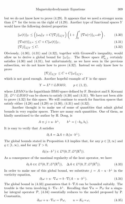
Magnetohydrodynamic Equations 309
but we do not know how to prove (4.29). It appears that we need a stronger normthan L∞ for the term on the right of (4.29). Another type of functional spaces Ywould have the following desired properties
‖ω(t)‖Y ≤(‖ω0‖Y + C‖∇j‖L1
tY
)(1 +
∫ t
0
‖∇u(τ)‖L∞dτ
), (4.30)
‖∇u(t)‖L∞ ≤ C + C‖ω(t)‖Y , (4.31)‖∇j‖L1
tY ≤ C. (4.32)
Obviously, (4.30), (4.31) and (4.32), together with Gronwall’s inequality, wouldallow us to derive a global bound for ‖ω‖Y . The Besov space B0
∞,1 certainlysatisfies (4.30) and (4.31), but unfortunately, as we have seen in the previoussubsection, we do not know how to prove (4.32). Instead we only know how toprove
‖∇j‖L1tY ≤ C + C‖ω‖L1
tY ,
which is not good enough. Another hopeful example of Y is the space
Y = Lp ∩ LBMO, p ∈ (1, 2),
where LBMO is the logarithmic BMO space defined by F. Bernicot and S. Keraani[3]. Lp∩LBMO can be shown to satisfy (4.30) and (4.31). We have not been ableto prove (4.32) for this space. We will continue to search for function spaces thatsatisfy either (4.28) and (4.29) or (4.30), (4.31) and (4.32).
Another thought is to make use of some of quantities that admit globalbounds in very regular spaces. There are many such quantities. One of them, askindly mentioned to the author by H. Dong, is
A ≡ j + u · b⊥, b⊥ = (−b2, b1).It is easy to verify that A satisfies
∂tA = ΔA+ ∂t(u · b⊥).
The global bounds stated in Proposition 4.3 implies that, for any p ∈ [2,∞) andq ∈ [1,∞), and for any T > 0,
∂t(u · b⊥) ∈ Lq(0, T ;Lp(R2)).
As a consequence of the maximal regularity of the heat operator, we have
∂tA ∈∈ Lq(0, T ;Lp(R2)), ΔA ∈ Lq(0, T ;Lp(R2)). (4.33)
In order to make use of this global bound, we substitute j = A − u · b⊥ in thevorticity equation,
∂tω + u · ∇ω = b · ∇(A− u · b⊥). (4.34)
The global bound in (4.33) guarantees that b · ∇A can be bounded suitably. Thetrouble is the term involving b · ∇u · b⊥. Recalling that ∇u = Pω for a singu-lar integral operator P , (4.34) essentially reduces to the model proposed by P.Constantin,
∂tω + u · ∇ω = Pω, u = K2 ∗ ω, (4.35)
310 Jiahong Wu
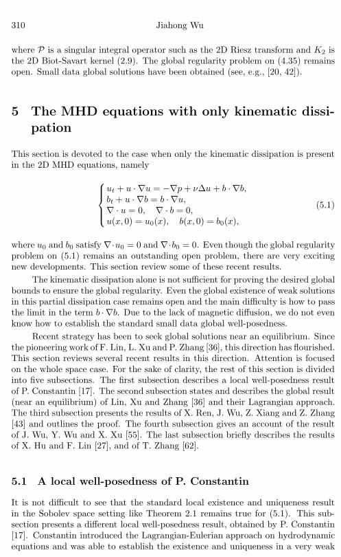
where P is a singular integral operator such as the 2D Riesz transform and K2 isthe 2D Biot-Savart kernel (2.9). The global regularity problem on (4.35) remainsopen. Small data global solutions have been obtained (see, e.g., [20, 42]).
5 The MHD equations with only kinematic dissi-pation
This section is devoted to the case when only the kinematic dissipation is presentin the 2D MHD equations, namely⎧⎪⎪⎨⎪⎪⎩
ut + u · ∇u = −∇p+ νΔu + b · ∇b,bt + u · ∇b = b · ∇u,∇ · u = 0, ∇ · b = 0,u(x, 0) = u0(x), b(x, 0) = b0(x),
(5.1)
where u0 and b0 satisfy ∇·u0 = 0 and ∇·b0 = 0. Even though the global regularityproblem on (5.1) remains an outstanding open problem, there are very excitingnew developments. This section review some of these recent results.
The kinematic dissipation alone is not sufficient for proving the desired globalbounds to ensure the global regularity. Even the global existence of weak solutionsin this partial dissipation case remains open and the main difficulty is how to passthe limit in the term b · ∇b. Due to the lack of magnetic diffusion, we do not evenknow how to establish the standard small data global well-posedness.
Recent strategy has been to seek global solutions near an equilibrium. Sincethe pioneering work of F. Lin, L. Xu and P. Zhang [36], this direction has flourished.This section reviews several recent results in this direction. Attention is focusedon the whole space case. For the sake of clarity, the rest of this section is dividedinto five subsections. The first subsection describes a local well-posedness resultof P. Constantin [17]. The second subsection states and describes the global result(near an equilibrium) of Lin, Xu and Zhang [36] and their Lagrangian approach.The third subsection presents the results of X. Ren, J. Wu, Z. Xiang and Z. Zhang[43] and outlines the proof. The fourth subsection gives an account of the resultof J. Wu, Y. Wu and X. Xu [55]. The last subsection briefly describes the resultsof X. Hu and F. Lin [27], and of T. Zhang [62].
5.1 A local well-posedness of P. Constantin
It is not difficult to see that the standard local existence and uniqueness resultin the Sobolev space setting like Theorem 2.1 remains true for (5.1). This sub-section presents a different local well-posedness result, obtained by P. Constantin[17]. Constantin introduced the Lagrangian-Eulerian approach on hydrodynamicequations and was able to establish the existence and uniqueness in a very weak

Magnetohydrodynamic Equations 311
functional setting. Consider the initial value problem for the system⎧⎪⎪⎪⎨⎪⎪⎪⎩∂tu+ u · ∇u = −∇p+ νΔu + ∇ · σ,∇ · u = 0,∂tσ + u · ∇σ = F (∇u, σ),u(x, 0) = u0(x), σ(x, 0) = σ0(x),
(5.2)
where F is a quadratic function of its variables.
Theorem 5.1. Let 0 < α < 1, 1 < p <∞, let u0 ∈ C1+α ∩ Lp be divergence-freeand σ0 ∈ Cα ∩ Lp.
(A) There exists T > 0 and a solution (u, σ) of (5.2) with u ∈ L∞(0, T ;C1+α∩Lp)and with σ ∈ Lip(0, T ;Cα ∩ Lp).
(B) Two solutions uj ∈ L∞(0, T ;C1+α∩Lp) and σj ∈ Lip(0, T ;Cα∩Lp), j = 1, 2obey the strong Lipschitz bound
‖∂tX2 − ∂tX1‖L∞(0,T ;C1+α∩Lp) + ‖∂tτ2 − ∂tτ1‖L∞(0,T ;Cα∩Lp)
≤ C(T ) (‖u2(0) − u1(0)‖C1+α∩Lp + ‖σ2(0) − σ1(0)‖Cα∩Lp) .
where Xj, j = 1, 2 denote the particle trajectories corresponding to uj, andτj , j = 1, 2 denote the Lagrangian counterparts of σj, or τj = σ ◦ Xj. Inparticular, two such solutions with the same initial data must coincide.
When (u, b) solves (5.1), (u, σ) with σ = b ⊗ b solves (5.2), as explained in(2.5). Theorem 5.1 provides a local well-posedness for the MHD equations (5.1).
5.2 The work of F. Lin, L. Xu and P. Zhang
The work of F. Lin, L. Xu and P. Zhang pioneered the study on the global well-posedness of (5.1) with smooth initial data which is close to some non-trivial steadystate. We first explain the mechanism on why the solutions of the perturbationequation near an equilibrium may exist for all time. As in (2.10), setting b = ∇⊥φallows us to write (5.1) as⎧⎪⎨⎪⎩
ut + u · ∇u = −∇p+ νΔu+ ∇⊥φ · ∇∇⊥φ,∇ · u = 0,φt + u · ∇φ = 0.
(5.3)
Clearly, (u, φ) = (0, x2) is a steady solution. Setting φ = x2 + ψ yields⎧⎪⎪⎨⎪⎪⎩∂tψ + u · ∇ψ + u2 = 0,∂tu1 + u · ∇u1 − νΔu1 + ∂1∂2ψ = −∂1p−∇ · (∂1ψ∇ψ),∂tu2 + u · ∇u2 − νΔu2 + ∂2
1ψ = −∂2p−∇ · (∂2ψ∇ψ),(ψ, u1, u2)(x, 0) = (ψ0(x), u10(x), u20(x)).
(5.4)
The aim is then to show that (5.4) possesses a unique global solution when theinitial data is sufficiently small. The most significant difference between (5.3) and

312 Jiahong Wu
(5.4) is that (5.4) contains an extra term u2 in the equation of ψ. This termappears to play a role in the process.
The approach of Lin, Xu and Zhang is Lagrangian. They reformulated (5.4)in Lagrangian coordinates. More precisely, they work with the displacement
Y (x, t) = X(x, t) − x
where X = X(x, t) be the particle trajectory determined by u. They then derivethe equation for Y , which satisfies⎧⎪⎨⎪⎩
Ytt − ΔyYt − ∂2y1Y = f(Y, q),
∇y · Y = ρ(Y ),Y (y, 0) = Y0(y), Yt(y, 0) = Y1(y),
where q(y, t) = (p+ |∇ψ|2) ◦X(y, t), f(Y, q) denotes a functions of Y and q, andρ(Y ) = J(Y2, Y1) with J being the Poisson bracket defined in (2.12). They thenestimate the Lagrangian velocity Yt in L1
tLipx, using the anisotropic Littlewood-Paley theory and anisotropic Besov space techniques. The estimates involved arevery delicate.
Due to their use of the Lagrangian coordinates, they need to impose a compat-ibility condition on the initial data ψ0, more precisely, ∂yψ0 and (1+∂yψ0,−∂xψ0)are admissible on 0 × R and supp ∂yψ0(·, y) ⊂ [−K,K] for some K. Here ∂yψ0
and (1 + ∂yψ0,−∂xψ0) are admissible on 0 × R if∫R
∂yψ0(Z(a, t))dt = 0 for all a ∈ 0 × R,
where Z is the particle trajectory defined by (1+∂yψ0,−∂xψ0). Their main resultcan be stated as follows.
Theorem 5.2. Given u0 and ψ0 satisfying (u0,∇ψ0) ∈ Hs ∩ Hs2 with s1 > 1,s2 ∈ (−1,− 1
2 ) and s > s1 + 2, and
‖∇ψ0‖Hs1+2 ≤ ε0, ‖(∇ψ0, u0)‖Hs1+1∩Hs2 + ‖∂yψ0‖Hs1+2 ≤ ε0
for some ε0 small. Assume that ∂yψ0 and (1 + ∂yψ0,−∂xψ0) are admissible on0 × R and ∂yψ0(·, y) ⊂ [−K,K] for some K. Then (5.4) has a unique globalsolution (ψ, u, p).
5.3 The work of X. Ren, J. Wu, Z. Xiang and Z. Zhang
Motivated by the work of Lin, Xu and Zhang [36], Ren, Wu, Xiang and Zhang [43]examined the same issue via a different approach, namely the global well-posednesson the perturbed system⎧⎨⎩∂tψ + u · ∇ψ + u2 = 0,
∂tu1 + u · ∇u1 − νΔu1 + ∂1∂2ψ = −∂1p−∇ · (∂1ψ∇ψ),∂tu2 + u · ∇u2 − νΔu2 + ∂2
1ψ = −∂2p−∇ · (∂2ψ∇ψ).(5.5)

Magnetohydrodynamic Equations 313
The paper of Ren, Wu, Xiang and Zhang [43] is based on the Eulerian approachand employs direct energy estimates. In addition, [43] also investigates the large-time behavior of the solutions and verifies a numerical observation that the energyof the MHD equations is dissipated at a rate independent of the ohmic resistivity.
The functional setting is the anisotropic Sobolev spaces defined below.
Definition 5.3. Let σ, s ∈ R. The anisotropic Sobolev space Hσ,s(R2) is definedby
Hσ,s(R2) ={f ∈ S′(R2) : ‖f‖Hσ,s < +∞
},
where
‖f‖Hσ,s =∥∥∥{
2js2σk‖ΔjΔhkf‖L2
}j,k
∥∥∥2,
or, in terms of the Fourier transforms,
‖f‖Hσ,s =[∫
R2|ξ|2sξ2σ
1 |f(ξ)|2dξ] 1
2
.
We need the anisotropic Sobolev spaces to deal with the anisotropic natureof the equations here. It is not very difficult to show that (u1, u2, ψ) satisfiesa degenerate damped wave equation that exhibits anisotropicity. As derived indetail in the next subsection, the linear part of the equation is given by
utt − Δut − ∂21u = 0.
The characteristic equation satisfies
λ2 + |ξ|2λ+ ξ21 = 0,
which has two roots
λ± = −|ξ|2 ± √|ξ|4 − 4ξ212
.
As |ξ| → ∞,
λ−(ξ) → − ξ21|ξ|2 ∼
{−1, |ξ| ∼ |ξ1|,0, |ξ| � |ξ1|.
Therefore, the dissipative effect is weak in the case of |ξ| � |ξ1|.The main result of [43] can be stated as in the following theorem.
Theorem 5.4. Assume (∇ψ0, u0) ∈ H8(R2). Let s ∈ (0, 12 ). There exists a small
positive constant ε such that, if, (∇ψ0, u0) ∈ H−s,−s ∩ H−s,8(R2), and
‖(∇ψ0, u0)‖H8 + ‖(∇ψ0, u0)‖H−s,−s + ‖|(∇ψ0, u0)‖H−s,8 ≤ ε,
then (5.5) has a unique global solution (ψ, u) satisfying
(∇ψ, u) ∈ C([0,+∞);H8(R2)).
Moreover, the solution decays at the same rate as that for the linearized solutions,
‖∂kx∇ψ‖L2 + ‖∂k
xu‖L2 ≤ Cε(1 + t)−s+k2 ,
for any t ∈ [0,+∞) and k = 0, 1, 2.

314 Jiahong Wu
To help understand the proof of Theorem 5.4 and extract the necessary decayrates, we first examine the linearized version of (5.5). The following propositionholds.
Proposition 5.5. Consider the linearized equation⎧⎪⎪⎪⎨⎪⎪⎪⎩∂tu1 − Δu1 − ∂x1x2ψ = 0,∂tu2 − Δu2 + ∂x1x1ψ = 0,∂tψ + u2 = 0,u(x, 0) = u0(x), ψ(x, 0) = ψ0(x).
Assume (u0,∇ψ0) ∈ H4 and |D1|−su0 ∈ H1+s and |D1|−s∇ψ0 ∈ H1+s for s > 0,then, for k = 0, 1, 2,
‖∂kx1u‖L2 + ‖∂k
x1∇ψ‖L2 ≤ C(1 + t)−
k+s2 .
To explain why we need the functional setting in the Sobolev space withnegative indices, we provide the main lines of the proof for this proposition.
Proof. For small ε1 > 0, define
D0(t) = ‖u‖2L2 + ‖∇u‖2
L2 + ‖∇ψ‖2L2 + ‖∇2ψ‖2
L2 + 2ε1〈u2,∇ψ〉,H0(t) = ‖∇u‖2
L2 + ‖∇2u‖2L2 + ε1‖∇∂1ψ‖2
L2 − ε1‖∇u2‖2L2 − ε1〈Δu2,Δψ〉,
Es(t) = ‖|D1|−su‖2L2 + ‖|D1|−s∇ψ‖2
L2
+‖|D|1+s|D1|−su‖2L2 + ‖|D|1+s|D1|−s∇ψ‖2
L2 .
We can showd
dtD0(t) + CH0(t) ≤ 0,
d
dtEs(t) ≤ 0.
By interpolation inequalities,
D0(t) ≤ Es(t)1
1+sH0(t)s
1+s , H0(t) ≥ Es(0)−1sD0(t)1+
1s .
Thus,
d
dtD0(t) + CEs(0)−
1sD0(t)1+
1s ≤ 0
and consequently
E(t) ≤ (E(0)−1s + C(s)t)−s = E0
(E
1s0 C(s)t + 1
)−s
.
This completes the proof of Proposition 5.5.
We now return to the full nonlinear system (5.5) and outline the proof ofTheorem 5.4. The frame work to prove the global existence of small solutions isthe Bootstrap Principle. The following abstract bootstrap principle is taken fromthe book of T. Tao [46, p. 21].

Magnetohydrodynamic Equations 315
Lemma 5.6 (Abstract Bootstrap Principle). Let I be an interval. Let C(t) andH(t) be two statements related to t ∈ I. If C(t) and H(t) satisfy
(a) if H(t) is true, then C(t) is true for the same t,(b) if C(t1) is true, then H(t) is true for t in a neighborhood of t1,(c) if C(tk) is true for a sequence tk → t, then C(t) is true,(d) C(t) is true for at least one t0 ∈ I,
then, C(t) is true for all t ∈ I.
We only provide a sketch of the proof while the detailed proof can be foundin [43].
Proof of Theorem 5.4. The proof is divided into two main steps:
(1) The first step is to obtain decay rates under the assumption that the solutionis small.
(2) The second step is to show that the solution is even smaller if the initial datais small.
Then the Bootstrap Principle would imply that the solution remain small for alltime. The initial step is to show that, if (u,∇ψ) satisfies
‖(u(t),∇ψ(t))‖H4 ≤ δ
for sufficiently small δ > 0 and for t ∈ [0, T ], then we can show
d
dtD0 + CH0 ≤ 0 for t ∈ [0, T ],
where D0 and H0 are defined as in the proof of Proposition 5.5. To further theestimate, we define the higher-order counterparts of D0 and H0. For l = 1, 2, wedefine
Dl(t) =∑j,k
22lk(‖ΔjΔhku‖2
L2 + ‖ΔjΔhk∇u‖2
L2 + ‖ΔjΔhk∇ψ‖2
L2
+‖ΔjΔhk∇2ψ‖2
L2 + 2ε1〈ΔjΔhku2,ΔjΔh
kΔψ〉),
Hl(t) =∑j,k
22lk(‖ΔjΔhk∇u‖2
L2 + ‖ΔjΔhk∇2u‖2
L2 + ε1‖ΔjΔhk∇∂1ψ‖2
L2
−‖ΔjΔhk∇u2‖2
L2 − ε1〈ΔjΔhkΔu2,ΔjΔh
kΔψ〉).We then show that, for e(t) = ‖(u,∇ψ)‖H8∩H−s,−s∩H−s,8 , if
supt∈[0,T ]
e(t) ≤ δ
for some sufficiently small δ, then
d
dtDl(t) + CHl(t) ≤ 0, t ∈ [0, T ].

316 Jiahong Wu
In order to extract the decay rates from these differential inequalities, we also needto include some intermediate norms in the estimates. We further define
Es,s1 = ‖(u,∇ψ)‖2H−s,s1
+ ‖(u,∇ψ)‖2H−s,s1+1 ,
εs,k(t) = Es,0(t) + Es,s+k(t).
We then prove that, for sufficiently small δ > 0, if, for k = 0, 1, 2,
supt∈[0,T ]
e(t) ≤ δ, supt∈[0,T ]
εs,k(t) ≤ δ,
then‖∂l
x1(u,∇ψ)‖L2 + ‖∂l
x1(∇u,∇2ψ)‖L2 ≤ C(1 + t)−
l+s2 .
Finally we show that, for sufficiently small r0 > 0, if
e(0) = ‖(u0,∇ψ0)‖H8∩H−s,8∩H−s,−s ≤ r0,
then (u,∇ψ) satisfies
e(t) = ‖(u,∇ψ)‖H8∩H−s,8∩H−s,−s ≤ 2r0, Es(t) ≤ 2r0,
where Es(t) = E0,7(t) + Es,−s(t) + E7,0(t). Therefore, if we choose 2r0 < 12δ,
then our proof above implies e(t) < 12δ. This then fulfills the assumptions of the
Bootstrap Principle, which then concludes that e(t) < 12δ for all t ∈ [0, T ]. This
completes the proof of Theorem 5.4.
5.4 The work of J. Wu, Y. Wu and X. Xu
This subsection presents the work of J. Wu, Y. Wu and X. Xu [55], which studiedthe global well-posedness near an equilibrium for the 2D MHD type equations witha velocity damping term instead of the dissipation, namely⎧⎪⎪⎪⎨⎪⎪⎪⎩
∂t�u+ �u · ∇�u + �u+ ∇P = −div(∇φ⊗∇φ), (t, x, y) ∈ R+ × R2,
∂tφ+ �u · ∇φ = 0,∇ · �u = 0,�u|t=1 = �u0(x, y), φ|t=1 = φ0(x, y),
(5.6)
where �u = (u, v). The notation in this subsection is slightly different from theprevious subsections. We use �u for the 2D velocity, u and v for its components,and (x, y) for the coordinates of a 2D point. Their paper takes the dispersivenature of the perturbed equations into full consideration and makes use of thetools and techniques for dispersive type equations.
We again consider the perturbation near the equilibrium u = 0, φ = y. Sub-stituting φ = y + ψ in (5.6) yields⎧⎪⎪⎪⎨⎪⎪⎪⎩
∂tu+ u∂xu+ v∂yu+ u+ ∂xP = −Δψ∂xψ,
∂tv + u∂xv + v∂yv + v + ∂yP = −Δψ − Δψ∂yψ,
∂tψ + u∂xψ + v∂yψ + v = 0,∂xu+ ∂yv = 0,
(5.7)
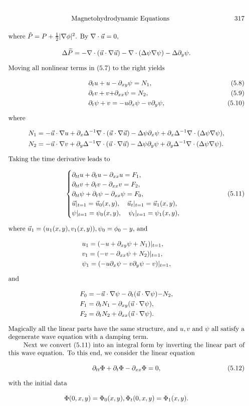
Magnetohydrodynamic Equations 317
where P = P + 12 |∇φ|2. By ∇ · �u = 0,
ΔP = −∇ · (�u · ∇�u) −∇ · (Δψ∇ψ) − Δ∂yψ.
Moving all nonlinear terms in (5.7) to the right yields
∂tu+ u− ∂xyψ = N1, (5.8)∂tv + v+∂xxψ = N2, (5.9)∂tψ + v = −u∂xψ − v∂yψ, (5.10)
where
N1 = −�u · ∇u+ ∂xΔ−1∇ · (�u · ∇�u) − Δψ∂xψ + ∂xΔ−1∇ · (Δψ∇ψ),
N2 = −�u · ∇v + ∂yΔ−1∇ · (�u · ∇�u) − Δψ∂yψ + ∂yΔ−1∇ · (Δψ∇ψ).
Taking the time derivative leads to⎧⎪⎪⎪⎪⎪⎪⎨⎪⎪⎪⎪⎪⎪⎩
∂ttu+ ∂tu− ∂xxu = F1,
∂ttv + ∂tv − ∂xxv = F2,
∂ttψ + ∂tψ − ∂xxψ = F0,
�u|t=1 = �u0(x, y), �ut|t=1 = �u1(x, y),ψ|t=1 = ψ0(x, y), ψt|t=1 = ψ1(x, y),
(5.11)
where �u1 = (u1(x, y), v1(x, y)), ψ0 = φ0 − y, and
u1 = (−u+ ∂xyψ +N1)|t=1,
v1 = (−v − ∂xxψ +N2)|t=1,
ψ1 = (−u∂xψ − v∂yψ − v)|t=1,
and
F0 = −�u · ∇ψ − ∂t(�u · ∇ψ)−N2,
F1 = ∂tN1 − ∂xy(�u · ∇ψ),F2 = ∂tN2 + ∂xx(�u · ∇ψ).
Magically all the linear parts have the same structure, and u, v and ψ all satisfy adegenerate wave equation with a damping term.
Next we convert (5.11) into an integral form by inverting the linear part ofthis wave equation. To this end, we consider the linear equation
∂ttΦ + ∂tΦ − ∂xxΦ = 0, (5.12)
with the initial data
Φ(0, x, y) = Φ0(x, y),Φt(0, x, y) = Φ1(x, y).

318 Jiahong Wu
Taking the Fourier transform on the equation (5.12), we have
∂ttΦ + ∂tΦ + ξ2Φ = 0, (5.13)
where the Fourier transform Φ is defined as
Φ(t, ξ, η) =∫
R2eixξ+iyηΦ(t, x, y)dxdy.
Solving (5.13) by a simple ordinary differential equation theory, we have
Φ(t, ξ, η)
=12
(e
(− 1
2 +√
14−ξ2
)t + e
(− 1
2−√
14−ξ2
)t)Φ0(ξ, η)
+1
2√
14 − ξ2
(e(−
12+
√14−ξ2)t − e(−
12−
√14−ξ2)t
)(12Φ0(ξ, η) + Φ1(ξ, η)
).
If we define the operators K0(t, ∂x),K1(t, ∂x) by
K0(t, ∂x)f(t, ξ, η) =12
(e
(− 1
2 +√
14−ξ2
)t + e
(− 1
2−√
14−ξ2
)t)f(t, ξ, η) (5.14)
and
K1(t, ∂x)f(t, ξ, η)
=1
2√
14 − ξ2
(e
(− 1
2+√
14−ξ2
)t − e
(− 1
2−√
14−ξ2
)t)f(t, ξ, η), (5.15)
where√−1 = i, then the solution Φ of the equation (5.12) can be written as
Φ(t, x, y) = K0(t, ∂x)Φ0 +K1(t, ∂x)(
12Φ0 + Φ1
).
Moreover, for the inhomogeneous equation,
∂ttΦ + ∂tΦ − ∂xxΦ = F,
with initial data Φ(x, 1) = Φ0(x), ∂tΦ(x, 1) = Φ1(x), the standard Duhamel for-mula implies
Φ(t, x, y) = K0(t, ∂x)Φ0 +K1(t, ∂x)(
12Φ0 + Φ1
)+
∫ t
1
K1(t− s, ∂x)F (s, x, y)ds. (5.16)
We need to estimate the decay properties of these kernel functions in orderto show that the terms in the integral representation remain small when the initialdata is sufficiently small. This lemma also indicates the anisotropicity in the decayestimates.

Magnetohydrodynamic Equations 319
Lemma 5.7. Let K0,K1 be defined in (5.14) and (5.15). Then
(1)∥∥|ξ|αKi(t, ·)
∥∥Lq
ξ(|ξ|≤ 12 )
� t−12 ( 1
q +α), for any α ≥ 0, 1 ≤ q ≤ ∞, i = 0, 1.
(2)∥∥∂tKi(t, ·)
∥∥Lq
ξ(|ξ|≤ 12 )
� t−1− 12q , i = 0, 1.
(3)∣∣Ki(t, ξ)
∣∣ � e−12 t, for any |ξ| ≥ 1
2 , i = 0, 1.(4)
∣∣〈ξ〉−1∂tK0(t, ξ)∣∣, ∣∣∂tK1(t, ξ)
∣∣ � e−12 t, for any |ξ| ≥ 1
2 .
Due to the complexity of the nonlinear terms, we need to choose a suitablefunctional setting for the initial data and for the solutions. Let X0 be the Banachspace defined by the following norm
‖(�u0, ψ0)‖X0 = ‖〈∇〉N (�u0,∇ψ0)‖L2xy
+‖〈∇〉6+(�u0, ψ0)‖L1xy
+ ‖〈∇〉6+(�u1, ψ1)‖L1xy,
where 〈∇〉 = (I −Δ)12 , N � 1 and a+ denotes a+ ε for small ε > 0. The solution
spaces X is defined by
‖(�u, ψ)‖X = supt≥1
{t−ε‖〈∇〉N (�u(t),∇ψ(t))‖2 + t
14 ‖〈∇〉3ψ‖2
+t14 ‖〈∇〉3ψ‖2 + t
32 ‖∂xxψ‖∞ + t
54 ‖〈∇〉2∂xxψ‖2 + t
32 ‖∂xxxψ‖2
+t32 ‖∂t�u‖∞ + t
54 ‖〈∇〉∂t�u‖2 + t‖〈∇〉∂x�u‖∞ + t
32 ‖∂x∂tv‖2
}.
Our main result can be stated as follows:
Theorem 5.8. There exists a small constant ε > 0 such that, if the initial datasatisfies ‖(�u0, ψ0)‖X0 ≤ ε, then (5.6) possesses a unique global solution (u, v, ψ) ∈X. Moreover, the following decay estimates hold
‖u(t)‖L∞x
� εt−1; ‖v(t)‖L∞x
� εt−32 ; ‖ψ(t)‖L∞
x� εt−
12 .
The proof of this theorem relies on the continuity argument, which is a con-sequence of the Bootstrap Principle.
Lemma 5.9 (Continuity Argument). Suppose that (�u, ψ) with the initial data(�u0, ψ0), satisfies
‖(�u, ψ)‖X � ‖(�u0, ψ0)‖X0 + C‖�u, ψ)‖βX (5.17)
with β > 1. Then, there exists r0 such that, if
‖(�u0, ψ0)‖X0 � r0,
then ‖(�u, ψ)‖X � 2r0.
Various tool estimates are obtained in [55]. The following is one of them.

320 Jiahong Wu
Proposition 5.10. Let K(t, ∂x) be a Fourier multiplier operator satisfying∥∥∂αxK(t, ξ)
∥∥L1
ξ(|ξ|≤ 12 )<∞,
∥∥K(t, ξ)∥∥
L∞ξ (|ξ|≥ 1
2 )<∞, α ≥ 0.
Then, for any space-time Schwartz function f ,∥∥∂αxK(t, ∂x)f
∥∥L∞
xy�
(∥∥∂αxK(t, ξ)
∥∥L1
ξ(|ξ|≤ 12 )
+∥∥K(t, ξ)
∥∥L∞
ξ (|ξ|≥ 12 )
)× ∥∥〈∇〉α+1+ε∂yf
∥∥L1
xy. (5.18)
Many delicate estimates on the kernel functions K0 and K1 have also beenestablished in [55]. To get a flavoring of how we proceed to bound the solutionin the solution space, we provide a segment of the estimates for one of the normsdefining the solution space. A lot more details can be found in [55]. By theDuhamel formula, namely (5.16),
ψ(t, x, y) = K0(t, ∂x)ψ0 +K1(t, ∂x)(
12ψ0 + ψ1
)+
∫ t
1
K1(t− s, ∂x)F0(s)ds.
Therefore,
‖〈∇〉∂xxψ‖∞ �‖〈∇〉∂xxK0(t)ψ0‖∞ +∥∥∥∥〈∇〉∂xxK1(t)
(12ψ0 + ψ1
)∥∥∥∥∞
+∥∥∥∥∫ t
1
〈∇〉∂xxK1(t− s)F0(s)ds∥∥∥∥∞.
By Proposition 5.10 and Lemma 5.7,
‖〈∇〉∂xxK0(t)ψ0‖∞�
(‖∂xxK0(t, ξ)‖L1ξ(|ξ|≤ 1
2 ) + ‖K0(t, ξ)‖L∞ξ (|ξ|≥ 1
2 )
)‖〈∇〉2+ε∂xx∂yψ0‖L1xy
�(t−
32 + e−t
)‖〈∇〉5+εψ0‖L1xy
� t−32 ‖〈∇〉5+εψ0‖X0 .
Similarly, we have∥∥∥∥〈∇〉∂xxK1(t)(
12ψ0 + ψ1
)∥∥∥∥∞
� t−32
∥∥∥∥〈∇〉5+ε
(12ψ0 + ψ1
)∥∥∥∥X0
.
Moreover, ∥∥∥∥∫ t
1
〈∇〉∂xxK1(t− s)F0(s)ds∥∥∥∥∞
�∫ t
1
‖∂xxK1(t− s)〈∇〉F0(s)‖∞ds
�∫ t
2
1
‖∂xxK1(t− s)〈∇〉F0(s)‖∞ds
+∫ t
t2
‖∂xK1(t− s)〈∇〉∂xF0(s)‖∞ds.
Magnetohydrodynamic Equations 321
The lines above illustrate how we bound the solution in one of the norms in thesolution space. More details can be found in [55].
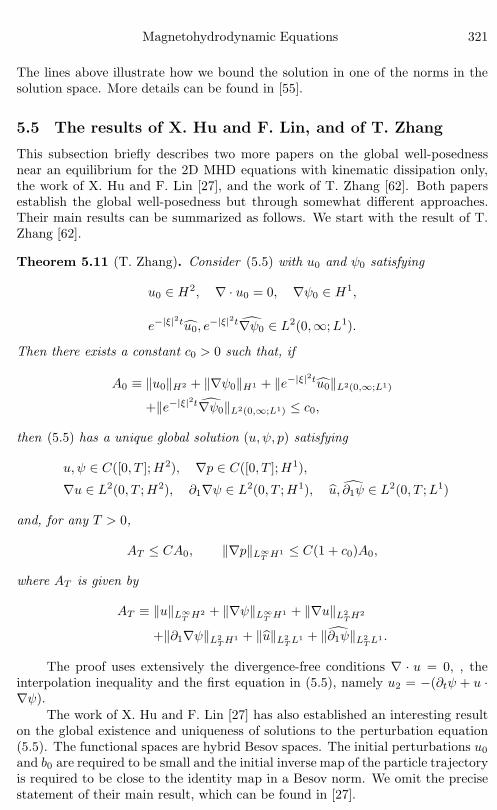
5.5 The results of X. Hu and F. Lin, and of T. Zhang
This subsection briefly describes two more papers on the global well-posednessnear an equilibrium for the 2D MHD equations with kinematic dissipation only,the work of X. Hu and F. Lin [27], and the work of T. Zhang [62]. Both papersestablish the global well-posedness but through somewhat different approaches.Their main results can be summarized as follows. We start with the result of T.Zhang [62].
Theorem 5.11 (T. Zhang). Consider (5.5) with u0 and ψ0 satisfying
u0 ∈ H2, ∇ · u0 = 0, ∇ψ0 ∈ H1,
e−|ξ|2tu0, e−|ξ|2t∇ψ0 ∈ L2(0,∞;L1).
Then there exists a constant c0 > 0 such that, if
A0 ≡ ‖u0‖H2 + ‖∇ψ0‖H1 + ‖e−|ξ|2tu0‖L2(0,∞;L1)
+‖e−|ξ|2t∇ψ0‖L2(0,∞;L1) ≤ c0,
then (5.5) has a unique global solution (u, ψ, p) satisfying
u, ψ ∈ C([0, T ];H2), ∇p ∈ C([0, T ];H1),
∇u ∈ L2(0, T ;H2), ∂1∇ψ ∈ L2(0, T ;H1), u, ∂1ψ ∈ L2(0, T ;L1)
and, for any T > 0,
AT ≤ CA0, ‖∇p‖L∞T H1 ≤ C(1 + c0)A0,
where AT is given by
AT ≡ ‖u‖L∞T H2 + ‖∇ψ‖L∞
T H1 + ‖∇u‖L2T H2
+‖∂1∇ψ‖L2T H1 + ‖u‖L2
T L1 + ‖∂1ψ‖L2T L1 .
The proof uses extensively the divergence-free conditions ∇ · u = 0, , theinterpolation inequality and the first equation in (5.5), namely u2 = −(∂tψ + u ·∇ψ).
The work of X. Hu and F. Lin [27] has also established an interesting resulton the global existence and uniqueness of solutions to the perturbation equation(5.5). The functional spaces are hybrid Besov spaces. The initial perturbations u0
and b0 are required to be small and the initial inverse map of the particle trajectoryis required to be close to the identity map in a Besov norm. We omit the precisestatement of their main result, which can be found in [27].
322 Jiahong Wu
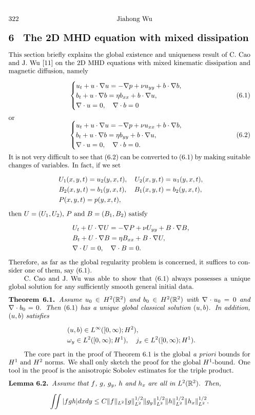
6 The 2D MHD equation with mixed dissipation
This section briefly explains the global existence and uniqueness result of C. Caoand J. Wu [11] on the 2D MHD equations with mixed kinematic dissipation andmagnetic diffusion, namely⎧⎪⎨⎪⎩
ut + u · ∇u = −∇p+ νuyy + b · ∇b,bt + u · ∇b = ηbxx + b · ∇u,∇ · u = 0, ∇ · b = 0
(6.1)
or ⎧⎪⎨⎪⎩ut + u · ∇u = −∇p+ νuxx + b · ∇b,bt + u · ∇b = ηbyy + b · ∇u,∇ · u = 0, ∇ · b = 0.
(6.2)
It is not very difficult to see that (6.2) can be converted to (6.1) by making suitablechanges of variables. In fact, if we set
U1(x, y, t) = u2(y, x, t), U2(x, y, t) = u1(y, x, t),B2(x, y, t) = b1(y, x, t), B1(x, y, t) = b2(y, x, t),P (x, y, t) = p(y, x, t),
then U = (U1, U2), P and B = (B1, B2) satisfy
Ut + U · ∇U = −∇P + νUyy +B · ∇B,Bt + U · ∇B = ηBxx +B · ∇U,∇ · U = 0, ∇ ·B = 0.
Therefore, as far as the global regularity problem is concerned, it suffices to con-sider one of them, say (6.1).
C. Cao and J. Wu was able to show that (6.1) always possesses a uniqueglobal solution for any sufficiently smooth general initial data.
Theorem 6.1. Assume u0 ∈ H2(R2) and b0 ∈ H2(R2) with ∇ · u0 = 0 and∇ · b0 = 0. Then (6.1) has a unique global classical solution (u, b). In addition,(u, b) satisfies
(u, b) ∈ L∞([0,∞);H2),ωy ∈ L2([0,∞);H1), jx ∈ L2([0,∞);H1).
The core part in the proof of Theorem 6.1 is the global a priori bounds forH1 and H2 norms. We shall only sketch the proof for the global H1-bound. Onetool in the proof is the anisotropic Sobolev estimates for the triple product.
Lemma 6.2. Assume that f , g, gy, h and hx are all in L2(R2). Then,∫∫|fgh|dxdy ≤ C‖f‖L2‖g‖1/2
L2 ‖gy‖1/2L2 ‖h‖1/2
L2 ‖hx‖1/2L2 .

Magnetohydrodynamic Equations 323
Any classical solution of (6.1) admits a global H1-bound.
Proposition 6.3. If (u, b) is a classical solution of (6.1), then
‖ω(t)‖22 + ‖j(t)‖2
2 + ν
∫ t
0
‖ωy(τ)‖22dτ + η
∫ t
0
‖jx(τ)‖22dτ
≤ C(ν, η)(‖ω0‖2
2 + ‖j0‖22
),
where C(ν, η) denotes a constant depending on ν and η only.
We start with the L2-bound:
‖u(t)‖22 + ‖b(t)‖2
2 + 2ν∫ t
0
‖uy(τ)‖22dτ + 2η
∫ t
0
‖bx(τ)‖22dτ ≤ ‖u0‖2
2 + ‖b0‖22.
To get the global H1-bound for (u, b), we consider ω and j satisfying
ωt + u · ∇ω = νωyy + b · ∇j,jt + u · ∇j = ηjxx + b · ∇ω
+2∂xb1(∂xu2 + ∂yu1) − 2∂xu1(∂xb2 + ∂yb1).
A simple energy estimate indicates that X(t) = ‖ω(t)‖22 + ‖j(t)‖2
2 obeys
12dX(t)dt
+ ν‖ωy‖22 + η‖jx‖2
2
≤ 2∫
(∂xb1(∂xu2 + ∂yu1) − ∂xu1(∂xb2 + ∂yb1)) jdxdy.
The terms on the right-hand side can be bounded as follows. By Lemma 6.2,∫|∂xb1||∂xu2||j|dxdy
≤ C‖∂xu2‖1/22 ‖∂xyu2‖1/2
2 ‖j‖1/22 ‖jx‖1/2
2 ‖∂xb1‖2
≤ ν
4‖∂xyu2‖2
2 +η
8‖jx‖2
2 + C‖∂xu2‖2‖∂xb1‖2‖j‖2
≤ ν
4‖ωy‖2
2 +η
8‖jx‖2
2 + C‖ω‖2‖∂xb1‖22‖j‖2
≤ ν
4‖ωy‖2
2 +η
8‖jx‖2
2 + C‖∂xb1‖22X(t).
Similarly,∫|∂xb1||∂yu1||j|dxdy ≤ ν
4‖ωy‖2
2 +η
8‖jx‖2
2 + C(‖∂xb1‖22 + ‖∂yu1‖2
2)‖j‖22.
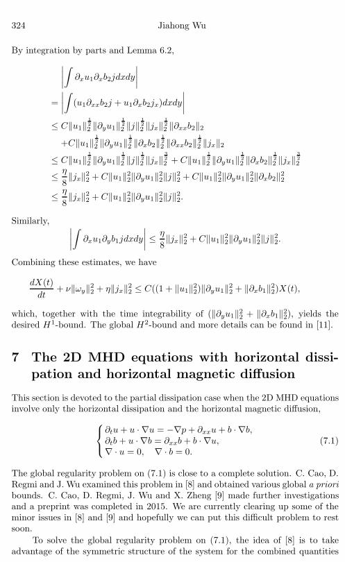
324 Jiahong Wu
By integration by parts and Lemma 6.2,∣∣∣∣∫ ∂xu1∂xb2jdxdy
∣∣∣∣=
∣∣∣∣∫ (u1∂xxb2j + u1∂xb2jx)dxdy∣∣∣∣
≤ C‖u1‖122 ‖∂yu1‖
122 ‖j‖
122 ‖jx‖
122 ‖∂xxb2‖2
+C‖u1‖122 ‖∂yu1‖
122 ‖∂xb2‖
122 ‖∂xxb2‖
122 ‖jx‖2
≤ C‖u1‖122 ‖∂yu1‖
122 ‖j‖
122 ‖jx‖
322 + C‖u1‖
122 ‖∂yu1‖
122 ‖∂xb2‖
122 ‖jx‖
322
≤ η
8‖jx‖2
2 + C‖u1‖22‖∂yu1‖2
2‖j‖22 + C‖u1‖2
2‖∂yu1‖22‖∂xb2‖2
2
≤ η
8‖jx‖2
2 + C‖u1‖22‖∂yu1‖2
2‖j‖22.
Similarly, ∣∣∣∣∫ ∂xu1∂yb1jdxdy
∣∣∣∣ ≤ η
8‖jx‖2
2 + C‖u1‖22‖∂yu1‖2
2‖j‖22.
Combining these estimates, we have
dX(t)dt
+ ν‖ωy‖22 + η‖jx‖2
2 ≤ C((1 + ‖u1‖22)‖∂yu1‖2
2 + ‖∂xb1‖22)X(t),
which, together with the time integrability of (‖∂yu1‖22 + ‖∂xb1‖2
2), yields thedesired H1-bound. The global H2-bound and more details can be found in [11].
7 The 2D MHD equations with horizontal dissi-
pation and horizontal magnetic diffusion
This section is devoted to the partial dissipation case when the 2D MHD equationsinvolve only the horizontal dissipation and the horizontal magnetic diffusion,⎧⎨⎩∂tu+ u · ∇u = −∇p+ ∂xxu+ b · ∇b,
∂tb + u · ∇b = ∂xxb+ b · ∇u,∇ · u = 0, ∇ · b = 0.
(7.1)
The global regularity problem on (7.1) is close to a complete solution. C. Cao, D.Regmi and J. Wu examined this problem in [8] and obtained various global a prioribounds. C. Cao, D. Regmi, J. Wu and X. Zheng [9] made further investigationsand a preprint was completed in 2015. We are currently clearing up some of theminor issues in [8] and [9] and hopefully we can put this difficult problem to restsoon.
To solve the global regularity problem on (7.1), the idea of [8] is to takeadvantage of the symmetric structure of the system for the combined quantities

Magnetohydrodynamic Equations 325
w± = u± b, ⎧⎪⎨⎪⎩∂tw
+ + (w− · ∇)w+ = −∇p+ ∂2xw
+,
∂tw− + (w+ · ∇)w− = −∇p+ ∂2
xw−,
∇ · w+ = 0, ∇ · w− = 0.(7.2)
The main difficulty to obtain a global bound for the H1-norm of w± is the ap-pearance of the L∞-norm of the horizontal components of w±, namely ‖w±
1 ‖2L∞ .
As a consequence, the global regularity problem boils down to control∫ T
0
‖w±1 ‖2
L∞dt or∫ T
0
(‖b1‖2L∞ + ‖u1‖2
L∞)dt.
Motivated by the work of Cao and Wu on the 2D Boussinesq equation with partialdissipation [13], the program in [8] is to obtain sharp bounds for ‖w±
1 ‖2Lq (in terms
of q), where 1 < q <∞. The symmetric formulation in (7.2) is more complex thanthe 2D Boussinesq equations. (7.2) consists of a system of two vector equationsand the interaction between them makes it more difficult mathematically. Forexample, the global H1 bound on the pressure established for the 2D Boussinesqequations has to be replaced by a global bound in a weaker space, namely in theHs-norm with s ∈ (0, 1). To deal with this more difficult situation, new tools suchas the triple product estimate involving fractional derivatives (see Lemma 7.2) areneeded to cope with the difficulty here.
If ‖w±1 ‖2
Lq does not grow too fast in q, say
‖w±1 ‖2
Lq ≤ Cq log(2 + q) or ‖(u1, b1)‖2Lq ≤ Cq log(2 + q), (7.3)
the preprint of Cao, Regmi, Wu and Zheng [9] was able to show that
Y (t) = ‖ω(·, t)‖2L2 + ‖j(·, t)‖2
L2
obeys the differential inequality
d
dtY (t) +
12(‖∂xω‖2
L2 + ‖∂xj‖2L2)
≤ C(1 + ‖(u1, b1)‖2L2 + ‖∂xu‖2
L2 + ‖∂xb‖2L2)Y (t)
+C
[sup
q∈[2,∞)
‖(u1, b1)‖Lq√q log(q)
]2
Y (t) log(e+ Y (t)) log(e+ log(e+ Y (t))).
The Osgood inequality then would imply a global bound for Y . The global H2-bound then follows as a consequence.
In order to prove (7.3), one needs a good global bound on the pressure p.The following global a priori bounds have been established in [8].
Proposition 7.1. Assume that (u0, b0) ∈ H2 and let (u, b) be the correspondingsolution of (7.1). Then, the following global a priori bounds hold:
(1) For any 1 ≤ r <∞, the first component (u1, b1) admits the global bound
‖(u1, b1)‖L2r ≤ C1eC2r3
,
where C1 and C2 are constants depending only on ‖(u0, b0)‖L2r .

326 Jiahong Wu
(2) Let p be the corresponding pressure. Let s ∈ (0, 1). Then, for any T > 0 andt ≤ T , the second component (u2, b2) and p admit the global bounds,
‖(u2, b2)‖L2r ≤ C r = 2, 3,
and, for any 1 < q ≤ 3,
‖p‖Lq ≤ C,
∫ T
0
‖p(τ)‖2Hsdτ ≤ C,
where C is a constant depending on T and the initial data only.
In order to obtain sharper global bounds for ‖(u1, b1)‖L2r , we need two toolestimates (see Lemma 4.1 and Lemma 4.2 in [8]).
Lemma 7.2. Let q ∈ [2,∞) and s ∈ (12 , 1]. Assume that f, g, ∂yg ∈ L2(R2),
h ∈ L2(q−1)(R2) and Λsxh ∈ L2(R2). Then,∣∣∣∣∫∫
R2fghdxdy
∣∣∣∣ ≤ C‖f‖2‖g‖ρ2‖∂yg‖1−ρ
2 ‖h‖ϑ2(q−1)‖Λs
xh‖1−ϑ2 , (7.4)
where ρ and ϑ are given by
ρ =12
+(2s− 1)(q − 2)
2(2s− 1)(q − 1) + 2, ϑ =
(2s− 1)(q − 1)(2s− 1)(q − 1) + 1
,
and Λsx denotes a fractional derivative with respect to x and is defined by
Λsxh(x) =
∫eix·ξ|ξ1|sh(ξ)dξ.
The following lemma allows us to bound the high frequency and low frequencyparts of a function in Hs (0 < s < 1) separately.
Lemma 7.3. Let f ∈ Hs(R2) with s ∈ (0, 1). Let R ∈ (0,∞). Denote by B(0, R)the ball centered at zero with radius R and by χB(0,R) the characteristic functionon B(0, R). Write
f = f+ f with f = F−1(χB(0,R)Ff) and f = F−1((1−χB(0,R))Ff), (7.5)
where F and F−1 denote the Fourier transform and the inverse Fourier transform,respectively. Then we have the following estimates for f and f .
(1) For a pure constant C0 (independent of s),
‖f‖∞ ≤ C0√1 − s
R1−s‖f‖Hs(R2), (7.6)
(2) For any 2 ≤ q <∞ satisfying 1−s− 2q < 0, there is a constant C1 independent
of s, q, R and f such that
‖f‖q ≤ C1qR1−s− 2
q ‖f‖Hs(R2). (7.7)
The key to obtain a sharper bound for ‖(u1, b1)‖L2r is to control the pressureassociated terms. The pressure is split into high frequency and low frequency partsaccording to (7.3) and bounded accordingly. More details can be found in [8].

Magnetohydrodynamic Equations 327
8 The MHD equations with fractional dissipation
This section summarizes recent results on the incompressible MHD equations withfractional dissipation⎧⎪⎪⎨⎪⎪⎩
ut + u · ∇u+ ν(−Δ)αu = −∇p+ b · ∇b,bt + u · ∇b+ η(−Δ)βb = b · ∇u,∇ · u = 0, ∇ · b = 0,u(x, 0) = u0(x), b(x, 0) = b0(x).
(8.1)
The aim is the global regularity of (8.1) for smallest possible parameters α ≥ 0and β ≥ 0. Since (8.1) was proposed for study in [51], there have been consider-able activities and the global well-posedness problem on (8.1) is now much betterunderstood (see, e.g., [12, 21, 31, 32, 47, 52, 53, 58, 59, 61]).
We summarize some of the results on (8.1). First of all, (8.1) with any α > 0and β > 0 always possesses a global weak solution in both 2D and 3D cases.
Theorem 8.1. Consider (8.1) with ν > 0, η > 0, α > 0 and β > 0. Let(u0, b0) ∈ L2(Rd) with ∇ · u0 = 0 and ∇ · b0 = 0. Then (8.1) has a global Leray-Hopf weak solution (u, b) satisfying, for any T > 0,
u ∈ L∞(0,∞;L2) ∩ L2(0,∞; Hα), b ∈ L∞(0,∞;L2) ∩ L2(0,∞; Hβ),
∂tu ∈ L4αd (0, T ;H−1), ∂tb ∈ L
4βd (0, T ;H−1).
A general result on the global existence and uniqueness of classical solutionsthat are valid for general d-dimensional MHD equations can be found in [51] and[53]. The result stated below is taken from [53].
Theorem 8.2. Consider the generalized incompressible magnetohydrodynamic(GMHD) equations of the form{
∂tu+ u · ∇u + L21u = −∇p+ b · ∇b, x ∈ Rd, t > 0,
∂tb+ u · ∇b+ L22b = b · ∇u, x ∈ Rd, t > 0,
(8.2)
where L1 and L2 are multiplier operators with symbols given by m1 and m2, namely
L1u(ξ) = m1(ξ)u(ξ), L2b(ξ) = m2(ξ)b(ξ).
Assume the initial data (u0, b0) ∈ Hs(Rd) with s > 1 + d2 , and ∇ · u0 = 0 and
∇ · b0 = 0. Assume the symbols m1 and m2 satisfy
m1(ξ) ≥ |ξ|αg1(ξ)
and m2(ξ) ≥ |ξ|βg2(ξ)
, (8.3)
where α and β satisfy
α ≥ 12
+d
4, β > 0, α+ β ≥ 1 +
d
2, (8.4)

328 Jiahong Wu
and g1 ≥ 1 and g2 ≥ 1 are radially symmetric, nondecreasing and satisfy∫ ∞
1
ds
s (g21(s) + g2
2(s))2= +∞. (8.5)
Then (8.2) has a unique global classical solution (u, b).
A special consequence of Theorem 8.2 is the global regularity for the specialdissipative operators
L21u =
(−Δ)α
log1/2(3 − Δ), L2
2u =(−Δ)β
log1/2(3 − Δ)
with
α ≥ 12
+d
4, β > 0, α+ β ≥ 1 +
d
2.
We remark that this result for the GMHD equations is not completely parallelto that for the generalized Navier-Stokes equations. In fact, the condition thatβ ≥ 1
2 + d4 is not imposed and (8.4) implies that it suffices to assume β > 0 when
α is sufficiently large.The borderline case α > 0 and β = 0 is studied by K. Yamazaki [60] and his
main result can be stated as follows.
Theorem 8.3. The 2D fractional MHD equations⎧⎪⎪⎨⎪⎪⎩ut + u · ∇u = −∇p− ν
(−Δ)2
log12 (3 − Δ)
u+ b · ∇b,bt + u · ∇b = b · ∇u,∇ · u = 0, ∇ · b = 0
(8.6)
always possess a unique global solutions when the initial data is sufficiently smooth.
Several papers have been exclusively devoted to the global regularity problemin the 2D case. As already described in Subsection 4, the fractional 2D MHD equa-tions with α = 0 (or ν = 0) and β > 1 have been shown to possess a unique globalsolution for any sufficiently smooth data [12]. The paper of [21] has establishedthe global regularity of (8.1) with any α > 0 and β = 1.
The global regularity problem on (8.1) with β < 1 and α+β < 2 is currentlyopen.
Acknowledgments
J. Wu was partially supported by National Science Foundation grants DMS 1209153and DMS 1614246, by the AT&T Foundation at Oklahoma State University, andby National Natural Sciences Foundation of China (No. 11471103, a grant awardedto Professor B. Yuan).

Magnetohydrodynamic Equations 329
References
[1] H. Bahouri, J.-Y. Chemin and R. Danchin, Fourier Analysis and NonlinearPartial Differential Equations, Springer, 2011.
[2] J. Bergh and J. Lofstrom, Interpolation Spaces, An Introduction, Springer-Verlag, Berlin-Heidelberg-New York, 1976.
[3] F. Bernicot and S. Keraani, On the global well-posedness of the 2D Eulerequations for a large class of Yudovich type data, Ann. Sci. Ec. Norm. Super.47 (2014), 559–576.
[4] D. Biskamp, Nonlinear Magnetohydrodynamics, Cambridge University Press,Cambridge, 1993.
[5] J. Bourgain and D. Li, Strong illposedness of the incompressible Euler equa-tion in integer Cm spaces, Geom. Funct. Anal., in press.
[6] J. Bourgain and D. Li, Strong Ill-posedness of the incompressible Euler equa-tion in borderline Sobolev spaces, arXiv:1307.7090 [math.AP] 26 Jul 2013.
[7] Y. Cai and Z. Lei, Global well-posedness of the incompressible magnetohy-drodynamics, arXiv:1605.00439 [math.AP] 2 May 2016.
[8] C. Cao, D. Regmi and J. Wu, The 2D MHD equations with horizontal dissipa-tion and horizontal magnetic diffusion, J. Differential Equations 254 (2013),2661–2681.
[9] C. Cao, D. Regmi, J. Wu and X. Zheng, Global regularity for the 2D magneto-hydrodynamics equations with horizontal dissipation and horizontal magneticdiffusion, preprint.
[10] C. Cao and J. Wu, Two regularity criteria for the 3D MHD equations, J.Differential Equations 248 (2010), 2263–2274.
[11] C. Cao and J. Wu, Global regularity for the 2D MHD equations with mixedpartial dissipation and magnetic diffusion, Adv. Math. 226 (2011), 1803–1822.
[12] C. Cao, J. Wu and B. Yuan, The 2D incompressible magnetohydrodynamicsequations with only magnetic diffusion, SIAM J. Math. Anal. 46 (2014), 588–602.
[13] C. Cao and J. Wu, Global regularity for the 2D anisotropic Boussinesq equa-tions with vertical dissipation, Arch. Rational Mech. Anal. 208 (2013), 985–1004.
[14] J.-Y. Chemin, D.S. McCormick, J.C. Robinson and J.L. Rodrigo, Local exis-tence for the non-resistive MHD equations in Besov spaces, arXiv:1503.01651[math.AP] 5 Mar 2015.
[15] Q. Chen, C. Miao and Z. Zhang, The Beale-Kato-Majda criterion for the 3Dmagneto-hydrodynamics equations, Comm. Math. Phys. 275 (2007), 861–872.
[16] Q. Chen, C. Miao and Z. Zhang, On the well-posedness of the ideal MHDequations in the Triebel-Lizorkin spaces, Arch. Ration. Mech. Anal. 195(2010), 561–578.
[17] P. Constantin, Lagrangian-Eulerian methods for uniqueness in hydrodynamicsystems, Adv. Math. 278 (2015), 67–102.
[18] P.A. Davidson, An Introduction to Magnetohydrodynamics, Cambridge Uni-versity Press, Cambridge, England, 2001.
[19] T.M. Elgindi and F. Rousset, Global regularity for some Oldroyd type models,

330 Jiahong Wu
arXiv:1308.1155 [math.AP] 3 Aug 2013.[20] T.M. Elgindi and K. Widmayer, Sharp decay estimates for an anisotropic
linear semigroup and applications to the surface quasi-geostrophic and inviscidBoussinesq systems, SIAM J. Math. Anal. 47 (2015), 4672–4684.
[21] J. Fan, G. Nakamura and Y. Zhou, Global Cauchy problem of 2D generalizedMHD equations, preprint.
[22] C.L. Fefferman, D.S. McCormick, J.C. Robinson and J.L. Rodrigo, Higherorder commutator estimates and local existence for the non-resistive MHDequations and related models, arXiv:1401.5018 [math.AP] 20 Jan 2014.
[23] C.L. Fefferman, D.S. McCormick, J.C. Robinson and J.L. Rodrigo, Local ex-istence for the non-resistive MHD equations in nearly optimal Sobolev spaces,arXiv:1602.02588 [math.AP] 8 Feb 2016.
[24] C. He and Z. Xin, Partial regularity of suitable weak solutions to the in-compressible magnetohydrodynamic equations, J. Funct. Anal. 227 (2005),113–152.
[25] C. He and Z. Xin, On the regularity of weak solutions to the magnetohydro-dynamic equations, J. Differential Equations 213 (2005), 235–254.
[26] L. He, L. Xu and P. Yu, On global dynamics of three dimensional mag-netohydrodynamics: nonlinear stability of Alfven waves, arXiv:1603.08205[math.AP] 27 Mar 2016.
[27] X. Hu and F. Lin, Global existence for two dimensional incompressible mag-netohydrodynamic flows with zero magnetic diffusivity, arXiv: 1405.0082v1[math.AP] 1 May 2014.
[28] Q. Jiu, C. Miao, J. Wu and Z. Zhang, The 2D incompressible Boussinesqequations with general critical dissipation, SIAM J. Mathematical Analysis46 (2014), 3426–3454.
[29] Q. Jiu and D. Niu, Mathematical results related to a two-dimensionalmagneto-hydrodynamic equations, Acta Math. Sci. Ser. B Engl. Ed. 26(2006), 744–756.
[30] Q. Jiu, D. Niu, J. Wu, X. Xu and H. Yu, The 2D magnetohydrodynamicequations with magnetic diffusion, Nonlinearity 28 (2015), 3935–3955.
[31] Q. Jiu and J. Zhao, A remark on global regularity of 2D generalized magne-tohydrodynamic equations, J. Math. Anal. Appl. 412 (2014), 478–484.
[32] Q. Jiu and J. Zhao, Global regularity of 2D generalized MHD equations withmagnetic diffusion, Z. Angew. Math. Phys. 66 (2015), 677–687.
[33] Z. Lei, On Axially Symmetric incompressible magnetohydrodynamics in threedimensions, J. Differential Equations 259 (2015), 3202–3215.
[34] Z. Lei and Y. Zhou, BKM’s criterion and global weak solutions for magne-tohydrodynamics with zero viscosity, Discrete Contin. Dyn. Syst. 25 (2009),575–583.
[35] P.G. Lemarie-Rieusset, Recent Developments in the Navier-Stokes Problem,Chapman & Hall/CRC Research Notes in Mathematics, 431, Chapman &Hall/CRC, Boca Raton, FL, 2002.
[36] F. Lin, L. Xu, and P. Zhang, Global small solutions to 2-D incompressibleMHD system, J. Differential Equations 259 (2015), 5440–5485.
[37] F. Lin and P. Zhang, Global small solutions to MHD type system (I): 3-D
Magnetohydrodynamic Equations 331
case, Comm. Pure. Appl. Math. 67 (2014), 531–580.[38] A. Majda and A. Bertozzi, Vorticity and Incompressible Flow, Cambridge
University Press, 2002.[39] C. Miao, J. Wu and Z. Zhang, Littlewood-Paley Theory and Applications to
Fluid Dynamics Equations, Monographs on Modern Pure Mathematics, 142,Science Press, Beijing, 2012.
[40] S.-I. Pai, Magnetogasdynamics and Plasma Dynamics, Springer-Verlag, Vi-enna, 1962.
[41] E. Priest and T. Forbes, Magnetic Reconnection, MHD Theory and Applica-tions, Cambridge University Press, Cambridge, 2000.
[42] F. Pusateri and K. Widmayer, On the global stability of a beta-plane equa-tion, arXiv:1610.03479 [math.AP] 11 Oct 2016.
[43] X. Ren, J. Wu, Z. Xiang and Z. Zhang, Global existence and decay of smoothsolution for the 2-D MHD equations without magnetic diffusion, J. FunctionalAnalysis 267 (2014), 503–541.
[44] T. Runst and W. Sickel, Sobolev Spaces of Fractional Order, Nemytskij Opera-tors and Nonlinear Partial Differential Equations, Walter de Gruyter, Berlin,New York, 1996.
[45] A. Stefnov and J. Wu, A global regularity result for the 2D Boussinesq equa-tions with critical dissipation, Journal d’Analyse Mathematique, accepted forpublication. Also posted in arXiv: 1411.1362 [math.AP] 5 Nov 2014.
[46] T. Tao, Nonlinear Dispersive Equations: Local and Global Analysis, CBMSregional conference series in mathematics, 2006.
[47] C. Tran, X. Yu and Z. Zhai, On global regularity of 2D generalized magneto-hydrodynamic equations, J. Differential Equations 254 (2013), 4194–4216.
[48] H. Triebel, Theory of Function Spaces II, Birkhauser Verlag, 1992.[49] W. Wang and Z. Zhang, Limiting case for the regularity criterion to the 3-
D magneto-hydrodynamics equations, J. Differential Equations 252 (2012),5751–5762.
[50] D. Wei and Z. Zhang, Global well-posedness of the MHD equations in ahomogeneous magnetic field, arXiv:1607.04397 [math.AP] 15 Jul 2016.
[51] J. Wu, Generalized MHD equations, J. Differential Equations 195 (2003),284–312.
[52] J. Wu, Regularity criteria for the generalized MHD equations, Comm. PartialDifferential Equations 33 (2008), 285–306.
[53] J. Wu, Global regularity for a class of generalized magnetohydrodynamicequations, J. Math. Fluid Mech. 13 (2011), 295–305.
[54] J. Wu and P. Zhang, The global regularity problem on the 2D magnetohy-drodynamic equations with magnetic diffusion only, work in progress.
[55] J. Wu, Y. Wu and X. Xu, Global small solution to the 2D MHD system witha velocity damping term, SIAM J. Math. Anal. 47 (2015), 2630–2656.
[56] L. Xu and P. Zhang, Global small solutions to three-dimensional incompress-ible MHD system, preprint.
[57] K. Yamazaki, On the global well-posedness of N -dimensional generalizedMHD system in anisotropic spaces, Adv. Differential Equations 19 (2014),201–224.

332 Jiahong Wu
[58] K. Yamazaki, Remarks on the global regularity of the two-dimensional mag-netohydrodynamics system with zero dissipation, Nonlinear Anal. 94 (2014),194–205.
[59] K. Yamazaki, On the global regularity of two-dimensional generalized mag-netohydrodynamics system, J. Math. Anal. Appl. 416 (2014), 99–111.
[60] K. Yamazaki, Global regularity of logarithmically supercritical MHD systemwith zero diffusivity, Appl. Math. Lett. 29 (2014), 46–51.
[61] B. Yuan and L. Bai, Remarks on global regularity of 2D generalized MHDequations, J. Math. Anal. Appl. 413 (2014), 633–640.
[62] T. Zhang, An elementary proof of the global existence and uniqueness the-orem to 2-D incompressible non-resistive MHD system, arXiv:1404.5681v1[math.AP] 23 Apr 2014.
[63] Y. Zhou and J. Fan, A regularity criterion for the 2D MHD system with zeromagnetic diffusivity, J. Math. Anal. Appl. 378 (2011), 169–172.

![2D Partial Unwinding-A Novel Non-linear Phase ... · tion among 2D Fourier series (2D-FS), 2D greedy algorithm (2D-GA) (or match pursuit) [26]–[31] on the product-Szego¨ dictionary,](https://img.pdfslide.net/doc/110x75/5f6242395a58451f7375be58/2d-partial-unwinding-a-novel-non-linear-phase-tion-among-2d-fourier-series-2d-fs.jpg)