Embed Size (px)
Citation preview

Solving General Linear Equations w/ Excel

Matrix Operations in Excel Excel has commands for:
Multiplication (mmult)…matrix multiplication
Transpose (transpose)…transpose a matrix
Determinant (mdeterm)…calc the determinate
Inverse (minverse)…generate the matrix inverse
Important to remember that these commands apply to an array of cells instead of to a single cell
When entering the command, you must identify the entire array where the answer will be displayed!

Practice Problem Find AB = C
(2 X 4) x (4 X 3) = ?
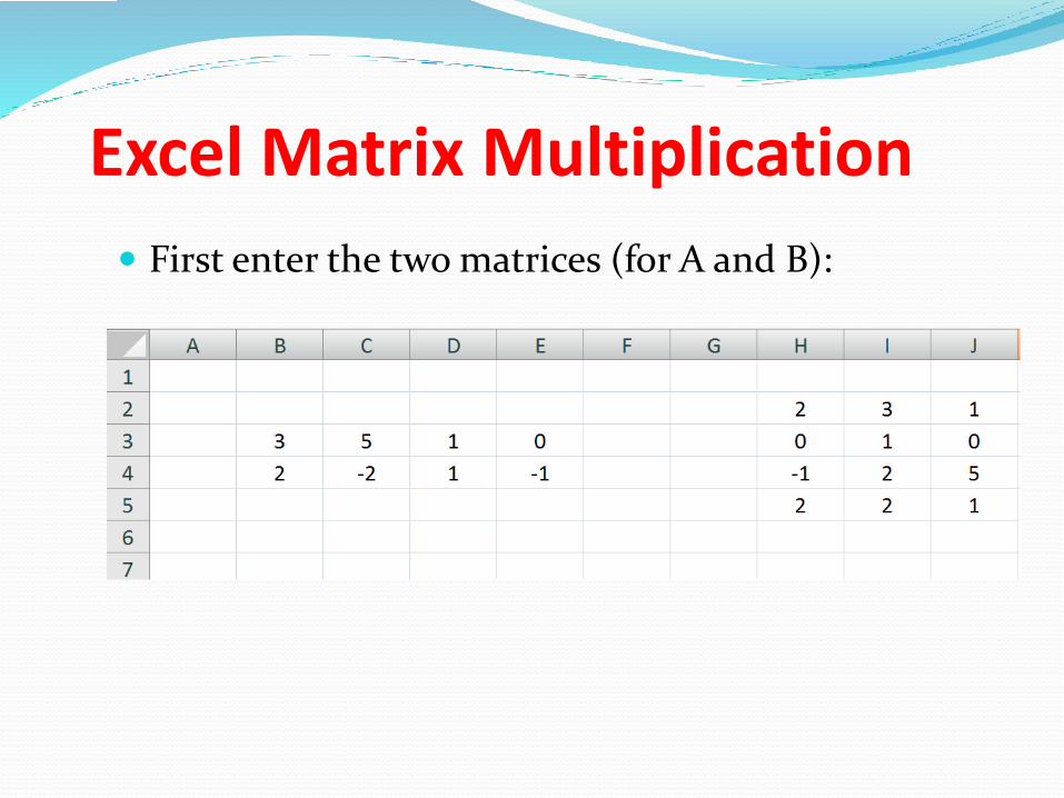
Excel Matrix Multiplication
First enter the two matrices (for A and B):
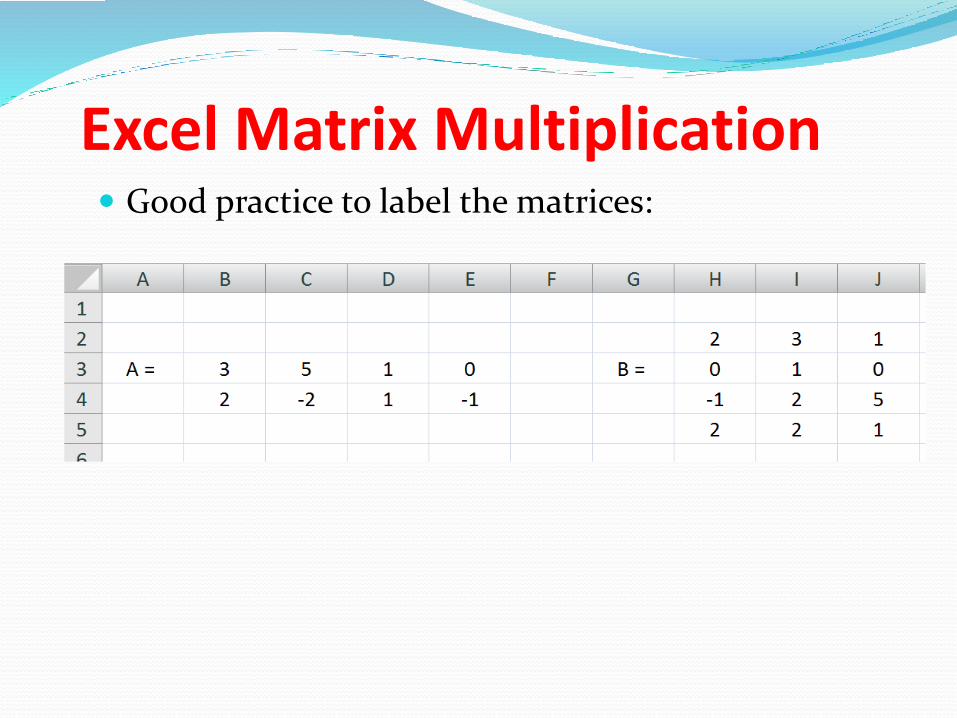
Excel Matrix Multiplication Good practice to label the matrices:

Excel Matrix Multiplication Shading and borders help the matrices stand out:
A x B = C….what size matrix must C be?

Excel Matrix Multiplication An array of cells for the product must be selected –
in this case, a 2 × 3 array: Select the cells – directly type mmult(array1,array2). You couldn’t paste the equation into the selected cells, they are in different dimensions.

Excel Matrix Multiplication The MMULT function has two arguments: the
ranges of cells to be multiplied. Remember that the order of multiplication is important.

Excel Matrix Multiplication Using the Enter key with an array command only returns an
answer in a single cell. Instead, use Ctrl + Shift + Enter keys with array functions (This only works when you highlight the solution area, then put the cursor in the top ‘function typing area’)
Try this out!

Excel Matrix Multiplication Answer cells formatted:

Excel Transpose Use Ctrl + Shift + Enter to input command
Try this out! (This only works when you highlight
the solution area, then put the cursor
in the top ‘function typing area’)

Excel Determinant Since determinant is a scalar, select a single cell
and use Enter to input command

Excel Matrix Inversion Remember that only square matrices can have
inverses

Excel Matrix Inversion Ctrl + Shift + Enter to input command

A X A-1 = I, the identity matrix:
Try this out: make a matrix – get its inverse matrix –
multiply these two matrix to get the identity matrix
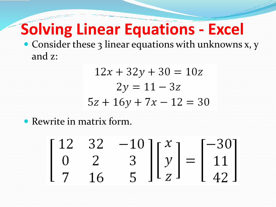
Solving Linear Equations - Excel Consider these 3 linear equations with unknowns x, y
and z:
Rewrite in matrix form.

MATLAB solution:
>> A=[12 32 -10; 0 2 3; 7 16 5];
>> b=[-30; 11; 42];
>> x=A\b
x =
7.0000
-2.0000
5.0000

Excel Solution Enter coefficient and constant matrices:
b =

Excel Solution Label and highlight cells for matrix of unknown
variables:
b =

Excel SolutionExcel does not have the convenient left division operator, so we must enter x = A-1b. Enter formula to invert Amatrix and multiply the result by the b matrix. This can be done in two steps or with nested commands:
b =

Excel Solution Apply formula to the selected array of cells by
pressing Ctrl + Shift + Enter:
b =

Exercises Solve the following sets of equations using
MATLAB and Excel and check the answer
0445
2
010423
zyx
zx
zyx
0425
02
23
02343
421
432
431
4321
xxx
xxx
xxx
xxxx

Solution 1
A = 3 -2 4 x B = 10
1 0 1 y 2
1 5 -4 z -4
x = 3.6
-2.8
-1.6
0445
2
010423
zyx
zx
zyx

Solution 2
0425
02
23
02343
421
432
431
4321
xxx
xxx
xxx
xxxx
A = 3 1 4 -1 x1 B = 23
3 0 1 1 x2 2
0 -2 1 1 x3 0
1 5 0 -2 x4 -4
x = 6.35
-8.52
-0.91
-16.13

So far we have been given different equations for a set of variables and solved for those variables:
2x1 + 3x2 = 12
4x1 – 3x2 = 6
Coefficients are known
x1, x2 are unknown
6
12
3- 4
3 2
2
1
x
x
It is common to have experimental measurements where the data are known but the equation or the equation coefficients are unknown.
Other uses of Ax=b and left-division

Fitting experimental data
Suppose someone is experimenting with a temperature controller. They apply a series of voltages and measure the resulting temperature.
Voltage Temperature
2 88.78
4 95.79
6 97.45
8 107.43
10 115.85

Fitting experimental data
You have reason to believe the relationship should
be linear, i.e.
T = c1V + c2
You know T, V
You want to find c1, c2
Notice this is the same equation as y = mx + b,
so we’re solving for slope and intercept.

Fitting experimental data First, let’s have a look at the data:
>> V = [2:2:10];
>> T = [88.78, 95.79, 97.45, 107.43, 115.85];
>> plot (V, T, ‘*’);
Not exactly a pretty straight line.
Could be
- The system really is not linear
- The voltage wasn’t exactly what
you thought
- The temperature measurement is
not accurate enough
- Etc.

Least Squares Fitting
• What line best represents the data?
x
y
• The best fit might not actually go through any points
• Forcing the line through a data point is risky

Least Squares Algorithm
• Least Squares minimizes the error between the line and the data points
• Find the line that minimizes the sum:
2)( i
ii mxy
ii mxy
x
y
Data
point
Line
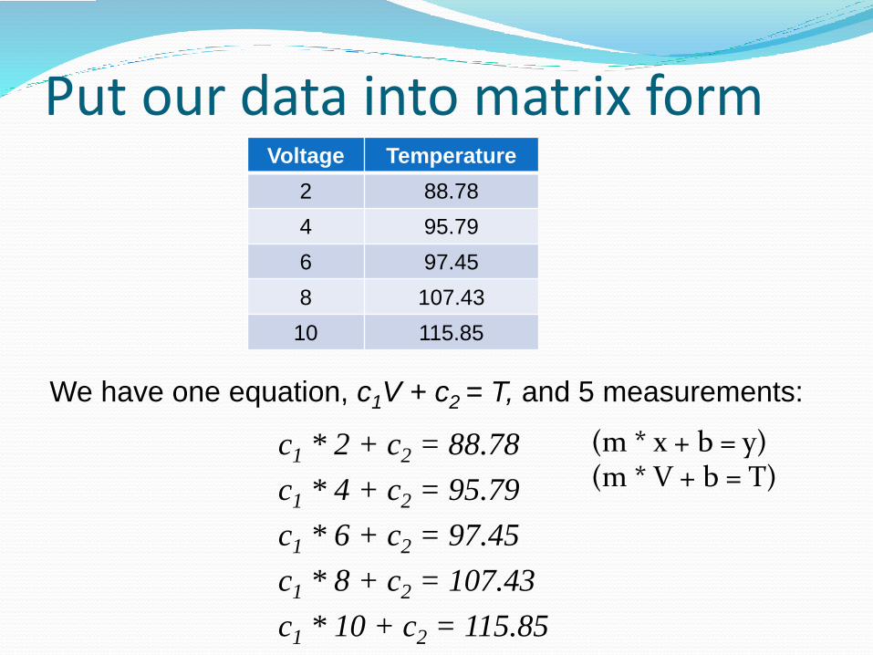
Put our data into matrix form
c1 * 2 + c2 = 88.78
c1 * 4 + c2 = 95.79
c1 * 6 + c2 = 97.45
c1 * 8 + c2 = 107.43
c1 * 10 + c2 = 115.85
Voltage Temperature
2 88.78
4 95.79
6 97.45
8 107.43
10 115.85
We have one equation, c1V + c2 = T, and 5 measurements:
(m * x + b = y)(m * V + b = T)

Put our data into matrix form
2 14 16810
111
𝑐1𝑐2
=
88.7895.7997.45107.43115.85
c1 * 2 + c2 = 88.78
c1 * 4 + c2 = 95.79
c1 * 6 + c2 = 97.45
c1 * 8 + c2 = 107.43
c1 * 10 + c2 = 115.85
Now it is in a familiar
form, Ax=b

This is over-determined2 14 16810
111
𝑐1𝑐2
=
88.7895.7997.45107.43115.85
Before we said we wanted equal number of
equations and unknowns for a unique solution.
Here we have 5 equations and 2 unknowns.
This would be redundant if the points were all
exactly on a line. Since they are not, this finds the
“best” (least-squares) compromise.

This is over-determined2 14 16810
111
𝑐1𝑐2
=
88.7895.7997.45107.43115.85
We can use the same left-division operator to
solve for c1, c2. MATLAB recognizes the system
is over-determined and switches to a least-squares
fit algorithm.
x = A\b
A x b

Solve % least square fit
clear all
close all
V=[2:2:10];
T=[88.78,95.79,97.45,107.43,115.85];
plot(V,T,'*’);
A=[2 1;4 1;6 1;8 1;10 1];
TT=transpose(T);
xx=A\TT;
hold on
line_vs=linspace(0,10,10);
line_ts=line_vs*xx(1)+xx(2);
plot(line_vs,line_ts);
x =
3.2890
81.3260
Our x vector components are c1, c2

Least squares fit to V, T data

Other function types Other types of functions can be fit using the same
technique. Consider this data
t y
0.0 0.82
0.3 0.72
0.8 0.63
1.1 0.60
1.6 0.55
2.3 0.50

Fitting a non-linear functionA linear fit looks like this:
You decide a decaying exponential function might be better

Fitting a non-linear function
The equation we want to try is
y(t) = c1 + c2e-t
Fitting a non-linear function does not mean the
system of equations is non-linear.
We will solve for c1, c2. This equation is still linear
with respect to c1, c2.

Put into matrix form
1 𝑒−0
1 𝑒−0.3
1111
𝑒−0.8
𝑒−1.1
𝑒−1.6
𝑒−2.3
𝑐1𝑐2
=
0.820.720.630.600.550.50
c1 + c2e-0 = 0.82
c1 + c2e-0.3 = 0.72
c1 + c2e-0.8 = 0.63
…

Solve clear all
close all
A=[1 exp(0); 1 exp(-0.3); 1 exp(-0.8); 1 exp(-1.1);1 exp(-1.6); 1 exp(-2.3)];
b=[0.82;0.72;0.63;0.60;0.55;0.50];
x1=[0;0.3;0.8;1.1; 1.6; 2.3];
plot(x1,b,'*');% plot the scattering dots
hold on
x=A\b;
line_x=linspace(0,2.5,20);
line_y=x(1)+x(2)*exp(-line_x);
plot(line_x,line_y);
x =
0.4760
0.3413
1 𝑒−0
1 𝑒−0.3
1111
𝑒−0.8
𝑒−1.1
𝑒−1.6
𝑒−2.3
𝑐1𝑐2
=
0.820.720.630.600.550.50
A x by(t) = 0.476 + 0.3413 e-t

New fit

Summary Curve fitting is a commonly-needed operation and
can be accomplished in Matlab as an Ax=b problem.
MATLAB’s left-division operator can be used to find
an exact solution in the case of equal number of
equations and unknowns.
It can also be used to perform a least-squares fit in
the case of more equations than unknowns.
Be aware though that the underlying algorithm is not
the same.


![Matrix - isabelle.in.tum.de filetranspose-matrix == Abs-matrix o transpose-infmatrix o Rep-matrix declare transpose-infmatrix-def [simp] lemma transpose-infmatrix-twice[simp]: transpose-infmatrix](https://img.pdfslide.net/doc/110x75/5e1c9d29dc47ca1d8a69b21f/matrix-abs-matrix-o-transpose-infmatrix-o-rep-matrix-declare-transpose-infmatrix-def.jpg)