Some Magnetic Field Properties of Ferrite Rods … · Some Magnetic Field Properties of Ferrite Rods Used for Small Ferrite Loaded Receiving Antennas Solved by the Moment Method--

Ferrite Rods by Moment Method

Some Magnetic Field Properties of Ferrite Rods Used for Small Ferrite Loaded Receiving Antennas Solved by the Moment Method-- presentation version 27 December 2001 --

by Ray L. Cross, BSEE, MSEEamateur radio WK0O

Introduction:

This paper is divided into Introduction, Derivation, and Calculation; the text for each section is color coded. It is not necessary to understand the derivation section to use the results. If you are not interested in the derivation you may skip directly to the calculation section.

This spreadsheet uses the Electromagnetic Field solution technique known as the "Moment Method" to find the magnetic field properties of ferrite rods that can be used for loading small receiving antennas. Not only fields in the rod from external fields, but the sheet calculates some factors of interest for the coils placed on the rod (such as inductance ratios and lengthy coil correction factors).

The technique used in this Mathcad has also been ported into an Excel spreadsheet to aid those who do not have Mathcad. In both cases field solution is assumed to be quasi-static -- a full wave solution has not yet been attempted as it is believed that the majority of cases will be covered with the quasi-static solution.

These spreadsheets are for analysis of a given design; as usual in these kind of problems, general synthesis of a new design is much harder. Guidance for the general design concept will be published elsewhere but this sheet should help in the refinement and validation of the design as well as providing the raw "data" from which new designs can be generated.

Started 10 April 1999 more experiments (no changes) 19 July 2000. Added end caps to the cylindrical current elements 15 December 2001. Other experiments (on side sheets) conducted in the intervening interval with triangle basis functions and other ideas are not shown here.

This effort was originally motivated by a paper by John Reed [1] which found discrepancies between some rod measurements and one form of a simplified theory of rod antennas. Although that particular problem may have been in the measurements, this motivated me to look into the current "state of the art" in calculating the fields in a ferrite rod antenna. It was apparent that there wasn't any readily available tools available to the average home experimenter beyond published charts and tables in some reference books. These charts and tables do not always cover the range of interest to experimenters. Additionally, there are several issues related to calculating the effects of voltage pickup and inductance that are not covered well.

Ray L. Cross 27 December 2001 1


is also a relative quantity. This permeability is considered to be an intrinsic material property of the ferrite and is that quantity which is measured when the ferrite is formed into a toroidal ring. The apparent permeability of the rod shape depends on the length to diameter ratio of the rod as well as the intrinsic material permeability.

µtororµiThe initial or toroidal permeability of the material expressed as:

µ0 4 π⋅ 107−

⋅:=

are relative quantities; this means for absolute calculation that they must be multiplied by the magnetic permeability of free space:

µcoilandµrod

It should be noted that:

= the inductance of the same coil in air with the ferrite rod removedLair

= the inductance of a particular coil in the presence of the ferrite rodLrod

= the uniform magnetic field in the absence of the ferrite rodBu_field

= the magnetic field in the exact center of the ferrite rod when long axis of the rod is inserted parallel to an uniform magnetic field

Brod

In the above formulas:

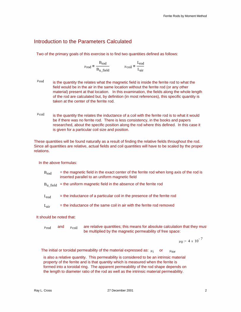
These quantities will be found naturally as a result of finding the relative fields throughout the rod. Since all quantities are relative, actual fields and coil quantities will have to be scaled by the proper relations.

is the quantity the relates the inductance of a coil with the ferrite rod is to what it would be if there was no ferrite rod. There is less consistency, in the books and papers researched, about the specific position along the rod where this defined. In this case it is given for a particular coil size and position.

µcoil

is the quantity the relates what the magnetic field is inside the ferrite rod to what the field would be in the air in the same location without the ferrite rod (or any other material) present at that location. In this examination, the fields along the whole length of the rod are calculated but, by definition (in most references), this specific quantity is taken at the center of the ferrite rod.

µrod

µcoilLrod

Lair=µrod

Brod

Bu_field=

Two of the primary goals of this exercise is to find two quantities defined as follows:

Introduction to the Parameters Calculated



Usually the procedure when working with calculations for antennas is to use µi in a formula or chart with the dimensions of the rod to determine µrod. Additional correction factors are required to determine the effect of the length of coil and placement of the coil of the rod for finding µcoil and the total voltage induced by the field. This procedure is summarized in reference [2] chapter 5 pages 5-2 to 5-9. Most of the references are relatively consistent in the determination of µrod from demagnetization factors. If formulas are used there are differences in the approximations for the demagnetization factor. There appears, however, to be a great diversity and perhaps even confusion for other desired coil/antenna quantities.

Some of the approximations (and data) related to the usual treatments of µrod are summarized in other spreadsheets. This spreadsheet, however, attempts to calculate the necessary information from fundamental principles. This was then compared with the previously existing data.

The principle references for obtaining equations and graphs to determine demagnetization factors and therefore µrod were Snelling, Polydoroff, Bozorth, etc. in references [1-6].



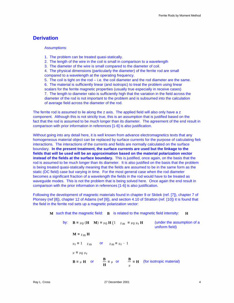
(for isotropic material)B

µH=or

B

Hµ=orB µ H⋅=

µ µ0 µr⋅=

χm µr 1−=orµr 1 χm+=

M χm H⋅=

(under the assumption of a uniform field)

B µ0 H M+( )⋅= µ0 H⋅ 1 χm+( )⋅= µ0 µr⋅ H⋅=by:

His related to the magnetic field intensity:Bsuch that the magnetic field: M

The ferrite rod is assumed to lie along the z axis. The applied field will also only have a z component. Although this is not strictly true, this is an assumption that is justified based on the fact that the rod is assumed to be much longer than its diameter. The agreement of the end result in comparison with prior information in references [1-6] is also justification.

Without going into any detail here, it is well known from advance electromagnetics texts that any homogeneous material object can be replaced by surface currents for the purpose of calculating field interactions. The interactions of the currents and fields are normally calculated on the surface boundary. In the present treatment, the surface currents are used but the linkage to the fields that will be used will be an approximation based on the material polarization vector instead of the fields at the surface boundary. This is justified, once again, on the basis that the rod is assumed to be much longer than its diameter. It is also justified on the basis that the problem is being treated quasi-statically meaning that the fields are assumed to be in the same form as the static (DC field) case but varying in time. For the most general case when the rod diameter becomes a significant fraction of a wavelength the fields in the rod would have to be treated as waveguide modes. This is not the problem that is being solved here. Once again the end result in comparison with the prior information in references [1-6] is also justification.

Following the development of magnetic materials found in chapter 9 or Skitek (ref. [7]), chapter 7 of Plonsey (ref [8]), chapter 12 of Adams (ref [9]), and section 4.10 of Stratton (ref. [10]) it is found that the field in the ferrite rod sets up a magnetic polarization vector:

Assumptions:

1. The problem can be treated quasi-statically. 2. The length of the wire in the coil is small in comparison to a wavelength3. The diameter of the wire is small compared to the diameter of coil.4. The physical dimensions (particularly the diameter) of the ferrite rod are small compared to a wavelength at the operating frequency.5. The coil is tight on the rod -- i.e. the coil diameter and the rod diameter are the same.6. The material is sufficiently linear (and isotropic) to treat the problem using linear scalars for the ferrite magnetic properties (usually true especially in receive cases)7. The length to diameter ratio is sufficiently high that the variation in the field across the diameter of the rod is not important to the problem and is subsumed into the calculation of average field across the diameter of the rod.

Derivation



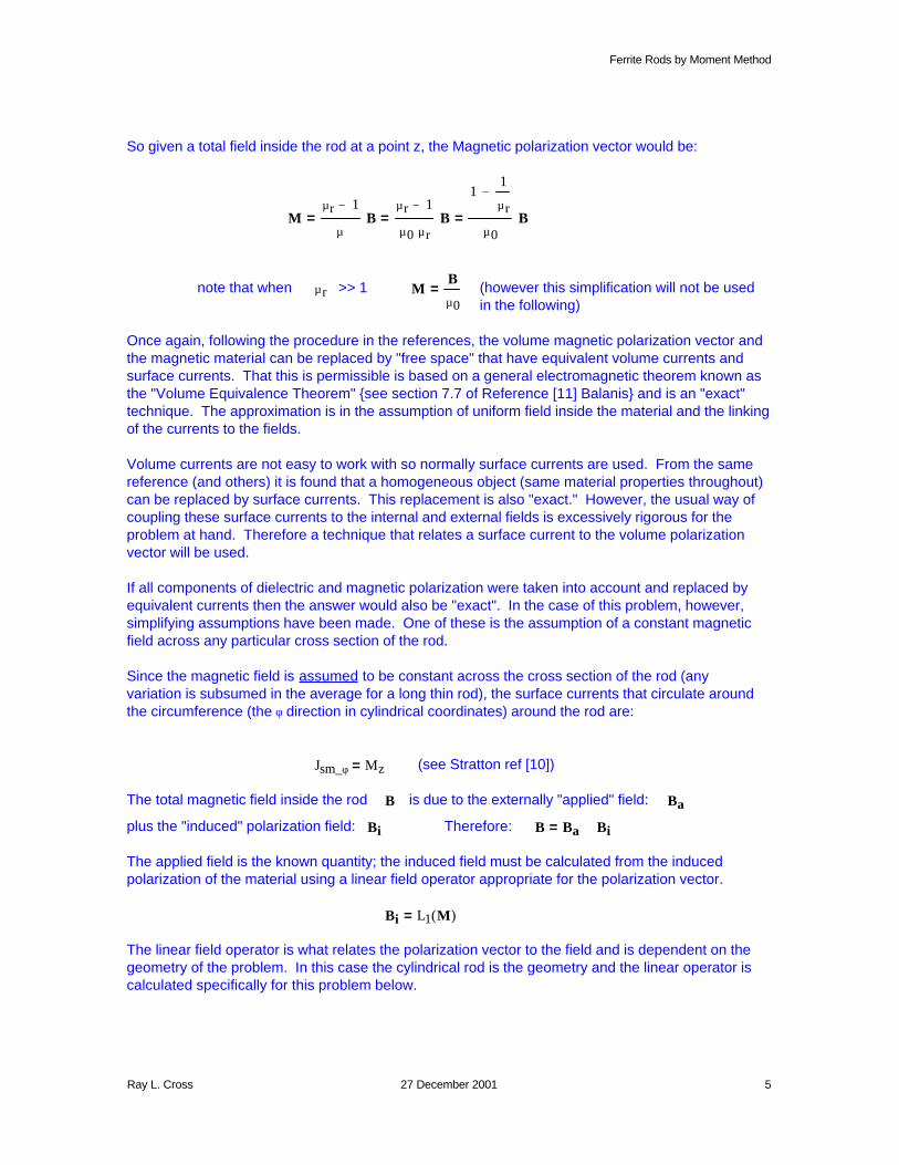
The linear field operator is what relates the polarization vector to the field and is dependent on the geometry of the problem. In this case the cylindrical rod is the geometry and the linear operator is calculated specifically for this problem below.

Bi L1 M( )=

The applied field is the known quantity; the induced field must be calculated from the induced polarization of the material using a linear field operator appropriate for the polarization vector.

B Ba Bi+=Therefore:Biplus the "induced" polarization field:

Bais due to the externally "applied" field:BThe total magnetic field inside the rod

(see Stratton ref [10])Jsm_φ Mz=

Once again, following the procedure in the references, the volume magnetic polarization vector and the magnetic material can be replaced by "free space" that have equivalent volume currents and surface currents. That this is permissible is based on a general electromagnetic theorem known as the "Volume Equivalence Theorem" {see section 7.7 of Reference [11] Balanis} and is an "exact" technique. The approximation is in the assumption of uniform field inside the material and the linking of the currents to the fields.

Volume currents are not easy to work with so normally surface currents are used. From the same reference (and others) it is found that a homogeneous object (same material properties throughout) can be replaced by surface currents. This replacement is also "exact." However, the usual way of coupling these surface currents to the internal and external fields is excessively rigorous for the problem at hand. Therefore a technique that relates a surface current to the volume polarization vector will be used.

If all components of dielectric and magnetic polarization were taken into account and replaced by equivalent currents then the answer would also be "exact". In the case of this problem, however, simplifying assumptions have been made. One of these is the assumption of a constant magnetic field across any particular cross section of the rod. Since the magnetic field is assumed to be constant across the cross section of the rod (any variation is subsumed in the average for a long thin rod), the surface currents that circulate around the circumference (the φ direction in cylindrical coordinates) around the rod are:

(however this simplification will not be used in the following)

MB

µ0=>> 1µrnote that when

Mµr 1−

µB⋅=

µr 1−

µ0 µr⋅B⋅=

11

µr−

µ0B⋅=

So given a total field inside the rod at a point z, the Magnetic polarization vector would be:



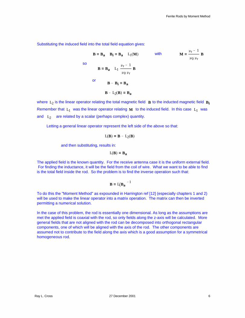
To do this the "Moment Method" as expounded in Harrington ref [12] (especially chapters 1 and 2) will be used to make the linear operator into a matrix operation. The matrix can then be inverted permitting a numerical solution.

In the case of this problem, the rod is essentially one dimensional. As long as the assumptions are met the applied field is coaxial with the rod, so only fields along the z-axis will be calculated. More general fields that are not aligned with the rod can be decomposed into orthogonal rectangular components, one of which will be aligned with the axis of the rod. The other components are assumed not to contribute to the field along the axis which is a good assumption for a symmetrical homogeneous rod.

B L Ba( ) 1−=

The applied field is the known quantity. For the receive antenna case it is the uniform external field. For finding the inductance, it will be the field from the coil of wire. What we want to be able to find is the total field inside the rod. So the problem is to find the inverse operation such that:

L B( ) Ba=

and then substituting, results in:

L B( ) B L2 B( )−=

Letting a general linear operator represent the left side of the above so that:

are related by a scalar (perhaps complex) quantity.L2and

wasL1to the induced field. In this caseMwas the linear operator relating

Substituting the induced field into the total field equation gives:

B Ba Bi+= Ba L1 M( )+= with Mµr 1−

µ0 µr⋅B⋅=

soB Ba L1

µr 1−

µ0 µr⋅B⋅

+=

orB Bi− Ba=

B L2 B( )− Ba=

where L2 is the linear operator relating the total magnetic field B to the inducted magnetic field Bi

Remember that L1



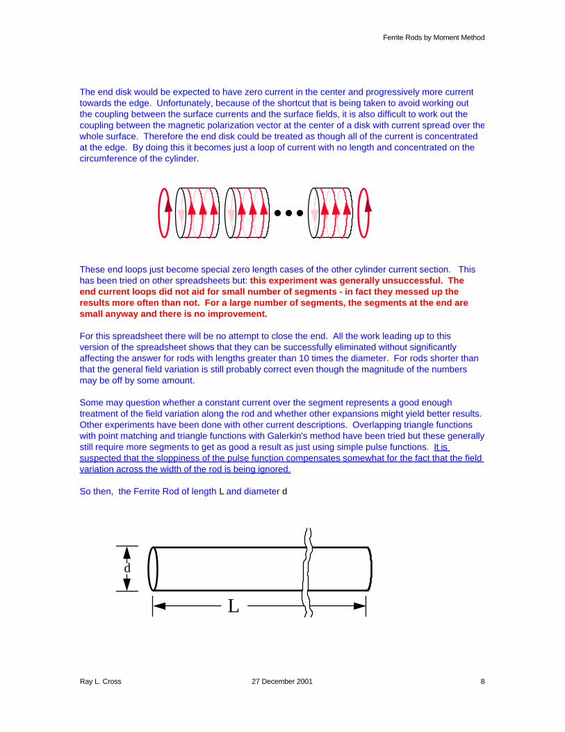
To complete the surface of the rod, ideally there would be end circular face place sections placed on each end of the stack of current cylinders. These would also be coupled magnetically to each other and all of the cylinder current elements. This has not been done in this treatment. No end caps have used in this spreadsheet. An alternate to the disks was considered and also rejected as discussed below.

ad

2=

and the radius

long LsegL

N=

for the basis functions.segmentsNand let the rod be segmented intodand the diameter beLLet the length of the rod be

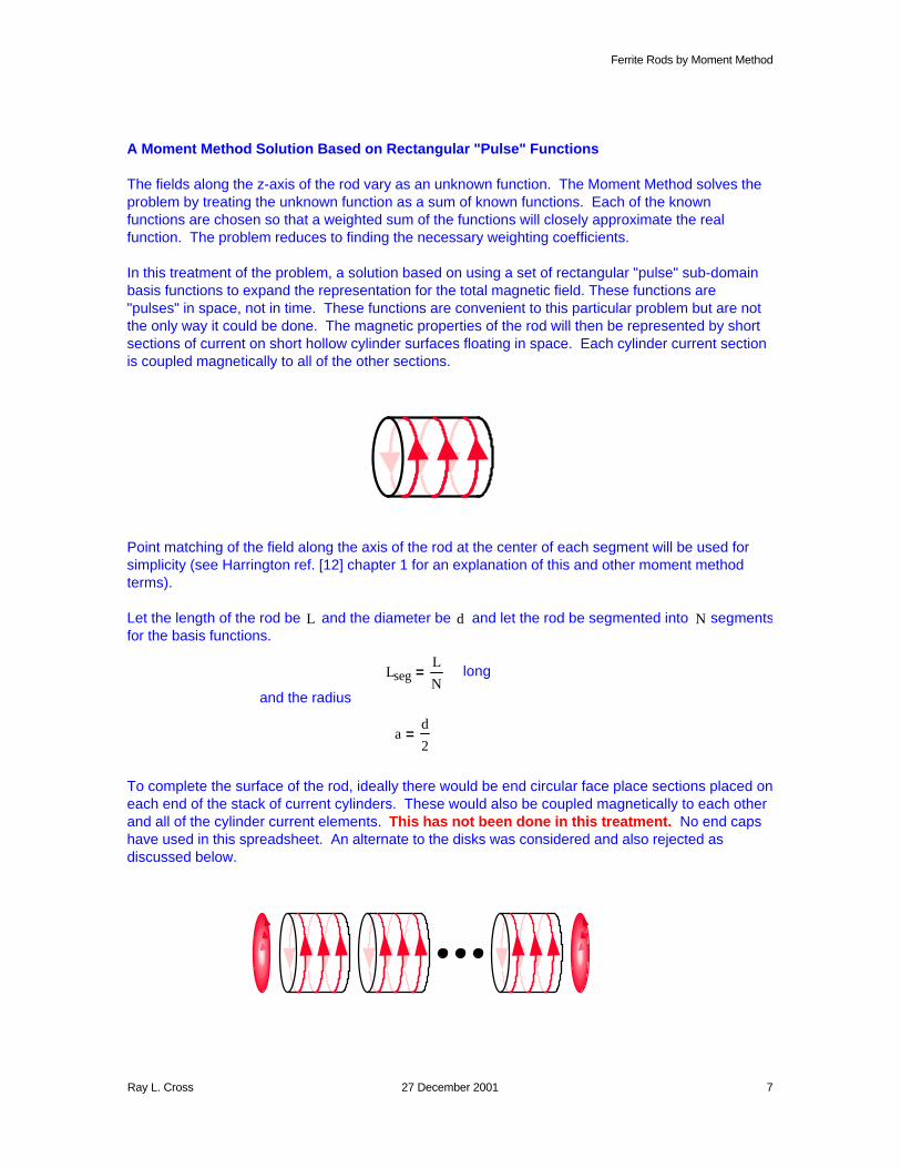
Point matching of the field along the axis of the rod at the center of each segment will be used for simplicity (see Harrington ref. [12] chapter 1 for an explanation of this and other moment method terms).

The fields along the z-axis of the rod vary as an unknown function. The Moment Method solves the problem by treating the unknown function as a sum of known functions. Each of the known functions are chosen so that a weighted sum of the functions will closely approximate the real function. The problem reduces to finding the necessary weighting coefficients.

In this treatment of the problem, a solution based on using a set of rectangular "pulse" sub-domain basis functions to expand the representation for the total magnetic field. These functions are "pulses" in space, not in time. These functions are convenient to this particular problem but are not the only way it could be done. The magnetic properties of the rod will then be represented by short sections of current on short hollow cylinder surfaces floating in space. Each cylinder current section is coupled magnetically to all of the other sections.

A Moment Method Solution Based on Rectangular "Pulse" Functions



The end disk would be expected to have zero current in the center and progressively more current towards the edge. Unfortunately, because of the shortcut that is being taken to avoid working out the coupling between the surface currents and the surface fields, it is also difficult to work out the coupling between the magnetic polarization vector at the center of a disk with current spread over the whole surface. Therefore the end disk could be treated as though all of the current is concentrated at the edge. By doing this it becomes just a loop of current with no length and concentrated on the circumference of the cylinder.

These end loops just become special zero length cases of the other cylinder current section. This has been tried on other spreadsheets but: this experiment was generally unsuccessful. The end current loops did not aid for small number of segments - in fact they messed up the results more often than not. For a large number of segments, the segments at the end are small anyway and there is no improvement.

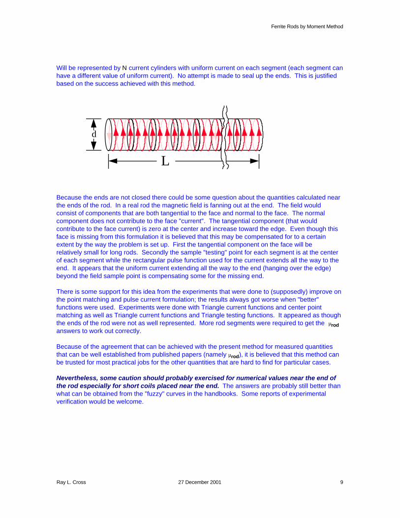
For this spreadsheet there will be no attempt to close the end. All the work leading up to this version of the spreadsheet shows that they can be successfully eliminated without significantly affecting the answer for rods with lengths greater than 10 times the diameter. For rods shorter than that the general field variation is still probably correct even though the magnitude of the numbers may be off by some amount.

Some may question whether a constant current over the segment represents a good enough treatment of the field variation along the rod and whether other expansions might yield better results. Other experiments have been done with other current descriptions. Overlapping triangle functions with point matching and triangle functions with Galerkin's method have been tried but these generally still require more segments to get as good a result as just using simple pulse functions. It is suspected that the sloppiness of the pulse function compensates somewhat for the fact that the field variation across the width of the rod is being ignored.

So then, the Ferrite Rod of length L and diameter d

L

d



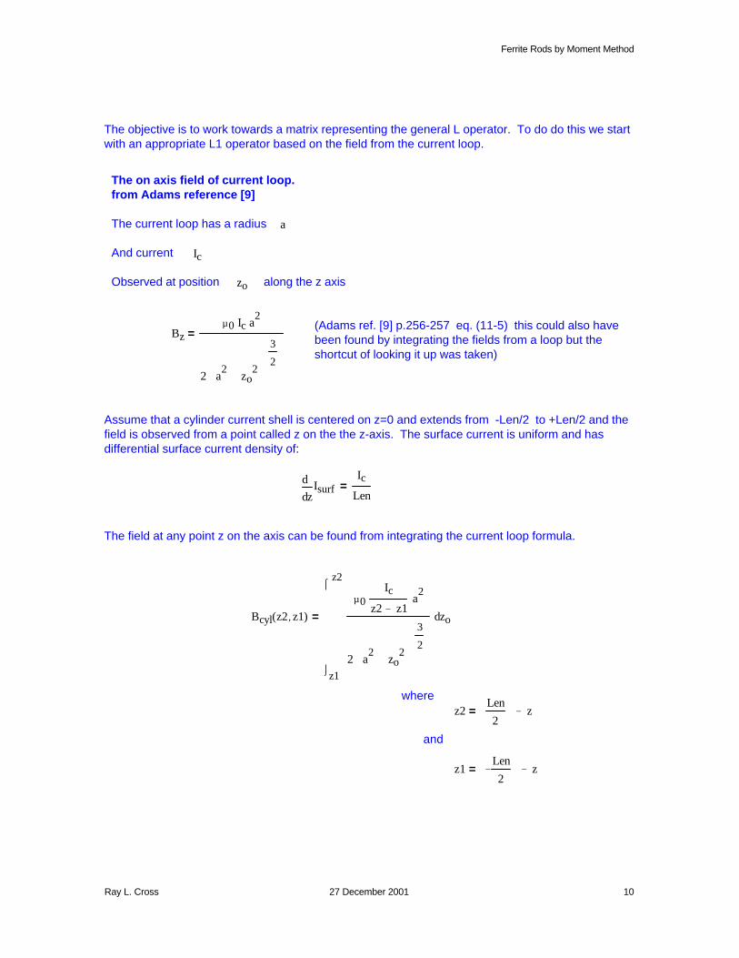
Will be represented by N current cylinders with uniform current on each segment (each segment can have a different value of uniform current). No attempt is made to seal up the ends. This is justified based on the success achieved with this method.

d

L

Because the ends are not closed there could be some question about the quantities calculated near the ends of the rod. In a real rod the magnetic field is fanning out at the end. The field would consist of components that are both tangential to the face and normal to the face. The normal component does not contribute to the face "current". The tangential component (that would contribute to the face current) is zero at the center and increase toward the edge. Even though this face is missing from this formulation it is believed that this may be compensated for to a certain extent by the way the problem is set up. First the tangential component on the face will be relatively small for long rods. Secondly the sample "testing" point for each segment is at the center of each segment while the rectangular pulse function used for the current extends all the way to the end. It appears that the uniform current extending all the way to the end (hanging over the edge) beyond the field sample point is compensating some for the missing end.

There is some support for this idea from the experiments that were done to (supposedly) improve on the point matching and pulse current formulation; the results always got worse when "better" functions were used. Experiments were done with Triangle current functions and center point matching as well as Triangle current functions and Triangle testing functions. It appeared as though the ends of the rod were not as well represented. More rod segments were required to get the µrod answers to work out correctly.

Because of the agreement that can be achieved with the present method for measured quantities that can be well established from published papers (namely µrod), it is believed that this method can be trusted for most practical jobs for the other quantities that are hard to find for particular cases.

Nevertheless, some caution should probably exercised for numerical values near the end of the rod especially for short coils placed near the end. The answers are probably still better than what can be obtained from the "fuzzy" curves in the handbooks. Some reports of experimental verification would be welcome.



z1Len

2−

z−=

and

z2Len

2

z−=where

Bcyl z2 z1,( )

z1

z2

zo

µ0Ic

z2 z1−⋅ a

2⋅

2 a2

zo2

+

3

2

⋅

⌠⌡

d=

The field at any point z on the axis can be found from integrating the current loop formula.

zIsurf

d

d

Ic

Len=

Assume that a cylinder current shell is centered on z=0 and extends from -Len/2 to +Len/2 and the field is observed from a point called z on the the z-axis. The surface current is uniform and has differential surface current density of:

Bzµ0 Ic⋅ a

2⋅

2 a2

zo2

+

3

2

⋅

=(Adams ref. [9] p.256-257 eq. (11-5) this could also have been found by integrating the fields from a loop but the shortcut of looking it up was taken)

along the z axiszoObserved at position

IcAnd current

aThe current loop has a radius

The on axis field of current loop.from Adams reference [9]

The objective is to work towards a matrix representing the general L operator. To do do this we start with an appropriate L1 operator based on the field from the current loop.



Ic_n

LenJsm_φ_n=

The φ directed surface current around the cylinder for a particular segment "n" is:

LenLD

N=for a rod with N segments the length becomes:

z1Len

2−

z−=andz2Len

2

z−=where

Bzcyl z2 z1, Len,( ) µ0Ic

Len⋅

z2

1 4 z22

⋅+

z1

1 4 z12

⋅+

−

⋅=

Bzcyl z2 z1, Len,( )1

8µ0⋅

Ic

Len⋅

z1

z2

zo1

1

4zo

2+

3

2

⌠⌡

d⋅=

for the current shell

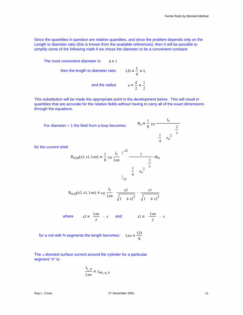
For diameter = 1 the field from a loop becomes: Bz1

8µ0⋅

Ic

1

4zo

2+

3

2

⋅=

This substitution will be made the appropriate point in the development below. This will result in quantities that are accurate for the relative fields without having to carry all of the exact dimensions through the equations.

ad

2=

1

2=and the radius

LDL

d= L=then the length to diameter ratio:

d 1=The most convenient diameter is:

Since the quantities in question are relative quantities, and since the problem depends only on the Length to diameter ratio (this is known from the available references), then it will be possible to simplify some of the following math if we chose the diameter to be a convenient constant.



z1LD

2 N⋅−

zdist−=andz2LD

2 N⋅

zdist−=

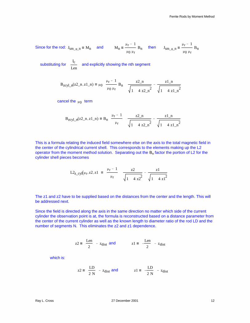
which is:

z1Len

2−

zdist−=andz2Len

2

zdist−=

Since the field is directed along the axis in the same direction no matter which side of the current cylinder the observation point is at, the formula is reconstructed based on a distance parameter from the center of the current cylinder as well as the known length to diameter ratio of the rod LD and the number of segments N. This eliminates the z2 and z1 dependence.

The z1 and z2 have to be supplied based on the distances from the center and the length. This will be addressed next.

L2z_cyl µr z2, z1,( )µr 1−

µr

z2

1 4 z22

⋅+

z1

1 4 z12

⋅+

−

⋅=

This is a formula relating the induced field somewhere else on the axis to the total magnetic field in the center of the cylindrical current shell. This corresponds to the elements making up the L2 operator from the moment method solution. Separating out the Bn factor the portion of L2 for the cylinder shell pieces becomes

Bzcyl_n z2_n z1_n,( ) Bnµr 1−

µr

⋅z2_n

1 4 z2_n2

⋅+

z1_n

1 4 z1_n2

⋅+

−

⋅=

termµ0cancel the

Bzcyl_n z2_n z1_n,( ) µ0µr 1−

µ0 µr⋅Bn⋅

⋅z2_n

1 4 z2_n2

⋅+

z1_n

1 4 z1_n2

⋅+

−

⋅=

and explicitly showing the nth segmentIc

Lensubstituting for

Jsm_φ_nµr 1−

µ0 µr⋅Bn⋅=thenMn

µr 1−

µ0 µr⋅Bn⋅=andJsm_φ_n Mn=Since for the rod:



Lis the matrix inverse ofL1−where

B L1−

Ba⋅=

is known, the solution to the total field isBasince

L B⋅ Ba=substituting

L I L2−( )=

matrix asLdefine theis the identity matrixIwhere

B I L2−( )⋅ Ba=

Bfactoring out the total field vector

B L2 B⋅− Ba=

substituting

B Bi− Ba=

Now the applied field is just the total field minus the induced field

Bi L2 B⋅=

The induced field vector (along the rod) is therefore the L2 matrix multiplied by the total field vector.

(If you feel like you are lost, it may be because I have skipped a few of the steps that are more clearly listed in the full treatment of the moment method - See Harrington in reference [12])

The objective here is to create an L2 matrix from the interactions from the n_th current element with the m_th observation point. The inducted field at all of the N observation points will then be related to the total field at the N observation points by a matrix multiplication.

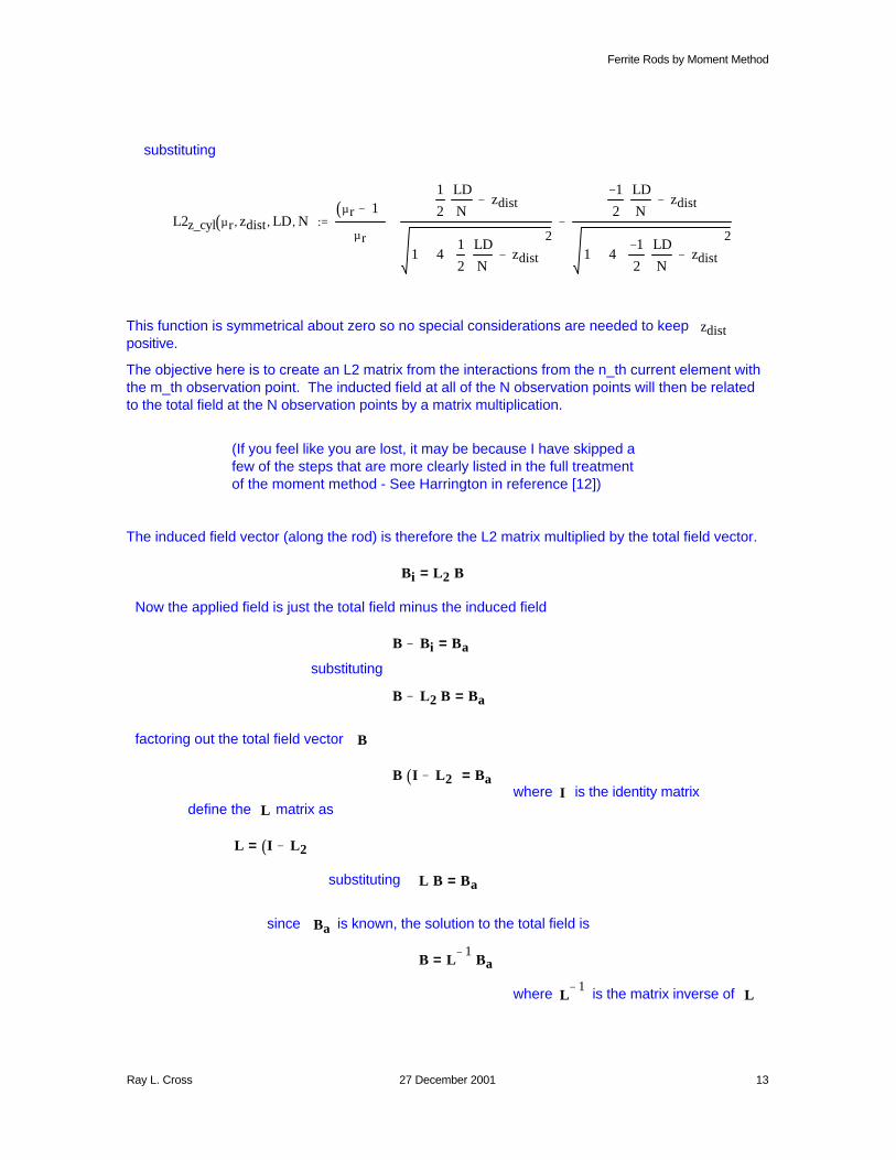
zdistThis function is symmetrical about zero so no special considerations are needed to keeppositive.

L2z_cyl µr zdist, LD, N,( )µr 1−( )

µr

1

2

LD

N⋅ zdist−

1 41

2

LD

N⋅ zdist−

2⋅+

1−

2

LD

N⋅ zdist−

1 41−

2

LD

N⋅ zdist−

2⋅+

−

⋅:=

substituting



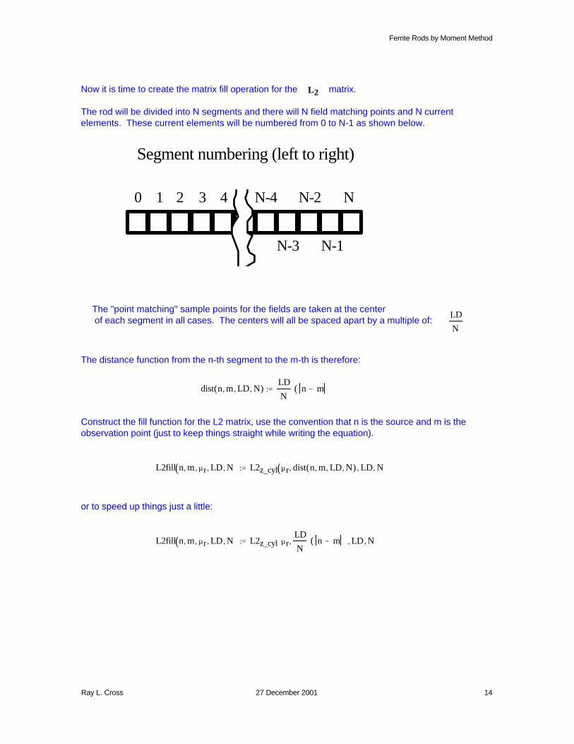
Now it is time to create the matrix fill operation for the L2 matrix.

The rod will be divided into N segments and there will N field matching points and N current elements. These current elements will be numbered from 0 to N-1 as shown below.

Segment numbering (left to right)

1 2 3 4

N-3

N-2

N-1

NN-40

The "point matching" sample points for the fields are taken at the center of each segment in all cases. The centers will all be spaced apart by a multiple of:

LD

N

The distance function from the n-th segment to the m-th is therefore:

dist n m, LD, N,( )LD

Nn m−( )⋅:=

Construct the fill function for the L2 matrix, use the convention that n is the source and m is the observation point (just to keep things straight while writing the equation).

L2fill n m, µr, LD, N,( ) L2z_cyl µr dist n m, LD, N,( ), LD, N,( ):=

or to speed up things just a little:

L2fill n m, µr, LD, N,( ) L2z_cyl µrLD

Nn m−( )⋅, LD, N,

:=



wavelengths long

(the experimental phase delay will then be) phasedelay n m, LD, N,( ) e

2− π⋅ i⋅ dist n m,(

⋅

:=

phasedelay 0 N 1+, LD, N,( ) 1=

L2fill_phase n m, µr, LD, N,( ) L2fill n m, µr, LD, N,( ) phasedelay n m, LD,(⋅:=

would have to change the name of the fill function below to use this ^^

end of experiment }

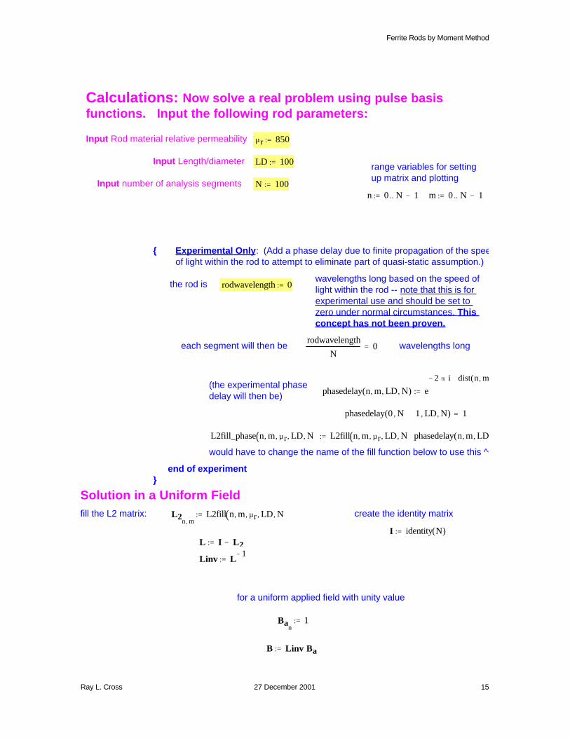
Solution in a Uniform Fieldfill the L2 matrix: L2

n m,L2fill n m, µr, LD, N,( ):= create the identity matrix

I identity N( ):=L I L2−:=

Linv L1−

:=

for a uniform applied field with unity value

Ban

1:=

B Linv Ba⋅:=

Calculations: Now solve a real problem using pulse basis functions. Input the following rod parameters:

Input Rod material relative permeability µr 850:=

Input Length/diameter LD 100:= range variables for setting up matrix and plotting

Input number of analysis segments N 100:=n 0 N 1−..:= m 0 N 1−..:=

{ Experimental Only: (Add a phase delay due to finite propagation of the speed of light within the rod to attempt to eliminate part of quasi-static assumption.)

wavelengths long based on the speed of light within the rod -- note that this is for experimental use and should be set to zero under normal circumstances. This concept has not been proven.

the rod is rodwavelength 0:=

each segment will then berodwavelength

N0=



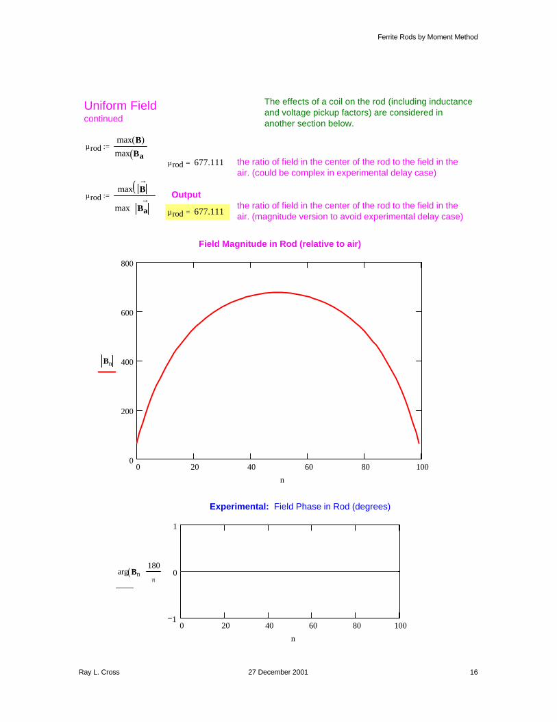
The effects of a coil on the rod (including inductance and voltage pickup factors) are considered in another section below.

Uniform Fieldcontinued

µrodmax B( )

max Ba( ):=

µrod 677.111= the ratio of field in the center of the rod to the field in the air. (could be complex in experimental delay case)

µrodmax B

→( )max Ba

→

:= Outputthe ratio of field in the center of the rod to the field in the air. (magnitude version to avoid experimental delay case)µrod 677.111=

Field Magnitude in Rod (relative to air)

0 20 40 60 80 1000

200

400

600

800

Bn

n

Experimental: Field Phase in Rod (degrees)

0 20 40 60 80 1001

0

1

arg Bn( )180

π⋅

n





z1

z2

z1

8

d2

1

4d2

⋅ z2

+

3

2

⋅

⌠⌡

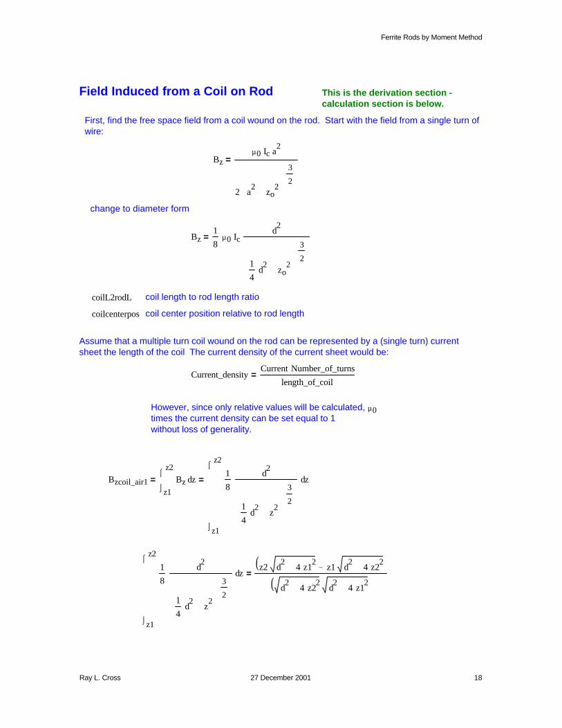
dz2 d

24 z1

2⋅+⋅ z1 d

24 z2

2⋅+⋅−( )

d2

4 z22

⋅+ d2

4 z12

⋅+⋅( )=

Bzcoil_air1z1

z2

zBz⌠⌡

d=

z1

z2

z1

8

d2

1

4d2

⋅ z2

+

3

2

⋅

⌠⌡

d=

times the current density can be set equal to 1 without loss of generality.

µ0However, since only relative values will be calculated,

Current_densityCurrent Number_of_turns⋅

length_of_coil=

Assume that a multiple turn coil wound on the rod can be represented by a (single turn) current sheet the length of the coil The current density of the current sheet would be:

coil center position relative to rod lengthcoilcenterpos

coil length to rod length ratiocoilL2rodL

Bz1

8µ0⋅ Ic⋅

d2

1

4d2

⋅ zo2

+

3

2

⋅=

change to diameter form

Bzµ0 Ic⋅ a

2⋅

2 a2

zo2

+

3

2

⋅

=

First, find the free space field from a coil wound on the rod. Start with the field from a single turn of wire:

This is the derivation section - calculation section is below.

Field Induced from a Coil on Rod



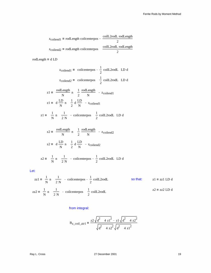
Bz_coil_air1z2 d

24 z1

2⋅+⋅ z1 d

24 z2

2⋅+⋅−

d2

4 z22

⋅+ d2

4 z12

⋅+⋅

=

from integral:

zz21

Nn⋅

1

2 N⋅+

coilcenterpos−1

2coilL2rodL⋅+=

z2 zz2 LD⋅ d⋅=

z1 zz1 LD⋅ d⋅=so that:zz11

Nn⋅

1

2 N⋅+

coilcenterpos−1

2coilL2rodL⋅−=

Let:

z21

Nn⋅

1

2 N⋅+

coilcenterpos−1

2coilL2rodL⋅−

LD⋅ d⋅=

z2 dLD

N⋅ n⋅

1

2d⋅

LD

N⋅+

zcoilend2−=

z2rodLength

Nn⋅

1

2

rodLength

N⋅+

zcoilend2−=

z11

Nn⋅

1

2 N⋅+

coilcenterpos−1

2coilL2rodL⋅+

LD⋅ d⋅=

z1 dLD

N⋅ n⋅

1

2d⋅

LD

N⋅+

zcoilend1−=

z1rodLength

Nn⋅

1

2

rodLength

N⋅+

zcoilend1−=

zcoilend2 coilcenterpos1

2coilL2rodL⋅+

LD⋅ d⋅=

zcoilend1 coilcenterpos1

2coilL2rodL⋅−

LD⋅ d⋅=

rodLength d LD⋅=

zcoilend2 rodLength coilcenterpos⋅coilL2rodL rodLength⋅

2+=

zcoilend1 rodLength coilcenterpos⋅coilL2rodL rodLength⋅

2−=



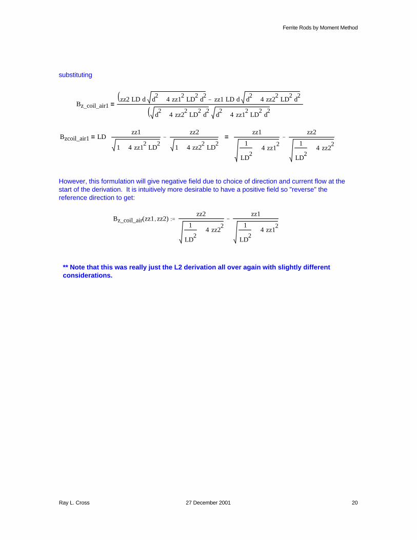
substituting

Bz_coil_air1zz2 LD⋅ d⋅ d

24 zz1

2⋅ LD

2⋅ d

2⋅+⋅ zz1 LD⋅ d⋅ d

24 zz2

2⋅ LD

2⋅ d

2⋅+⋅−( )

d2

4 zz22

⋅ LD2

⋅ d2

⋅+ d2

4 zz12

⋅ LD2

⋅ d2

⋅+⋅( )=

Bzcoil_air1 LDzz1

1 4 zz12

⋅ LD2

⋅+

zz2

1 4 zz22

⋅ LD2

⋅+

−

⋅=zz1

1

LD2

4 zz12

⋅+

zz2

1

LD2

4 zz22

⋅+

−

=

However, this formulation will give negative field due to choice of direction and current flow at the start of the derivation. It is intuitively more desirable to have a positive field so "reverse" the reference direction to get:

Bz_coil_air zz1 zz2,( )zz2

1

LD2

4 zz22

⋅+

zz1

1

LD2

4 zz12

⋅+

−:=

** Note that this was really just the L2 derivation all over again with slightly different considerations.



0 20 40 60 80 1001 .10

6

1 .10 5

1 .104

1 .103

0.01

0.1

1

Bzcoil_airn

n

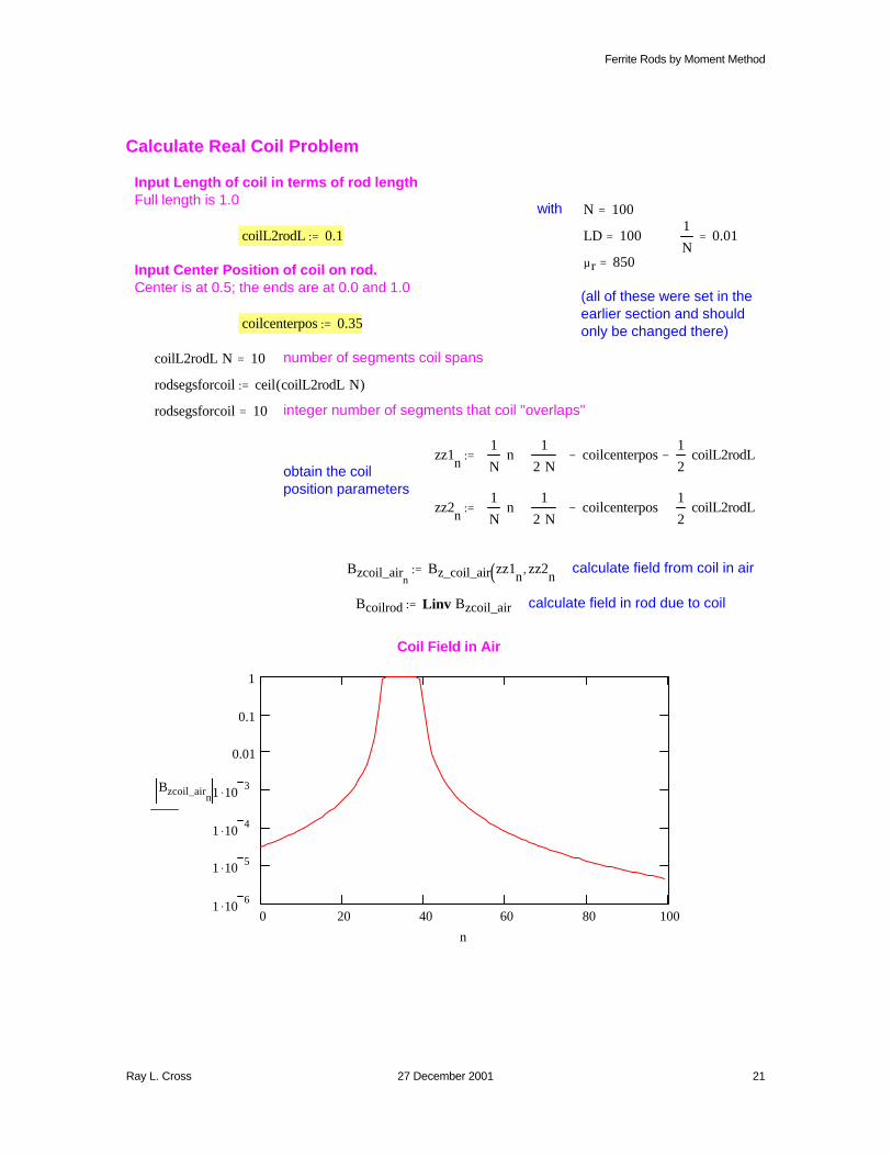
Coil Field in Air

calculate field in rod due to coilBcoilrod Linv Bzcoil_air⋅:=

calculate field from coil in airBzcoil_airn

Bz_coil_air zz1n

zz2n

,( ):=

zz2n

1

Nn⋅

1

2 N⋅+

coilcenterpos−1

2coilL2rodL⋅+:=

obtain the coil position parameters

zz1n

1

Nn⋅

1

2 N⋅+

coilcenterpos−1

2coilL2rodL⋅−:=

integer number of segments that coil "overlaps"rodsegsforcoil 10=

rodsegsforcoil ceil coilL2rodL N⋅( ):=

number of segments coil spanscoilL2rodL N⋅ 10=

coilcenterpos 0.35:=

(all of these were set in the earlier section and should only be changed there)

Input Center Position of coil on rod. Center is at 0.5; the ends are at 0.0 and 1.0

µr 850=

1

N0.01=LD 100=coilL2rodL 0.1:=

N 100=with

Input Length of coil in terms of rod lengthFull length is 1.0

Calculate Real Coil Problem



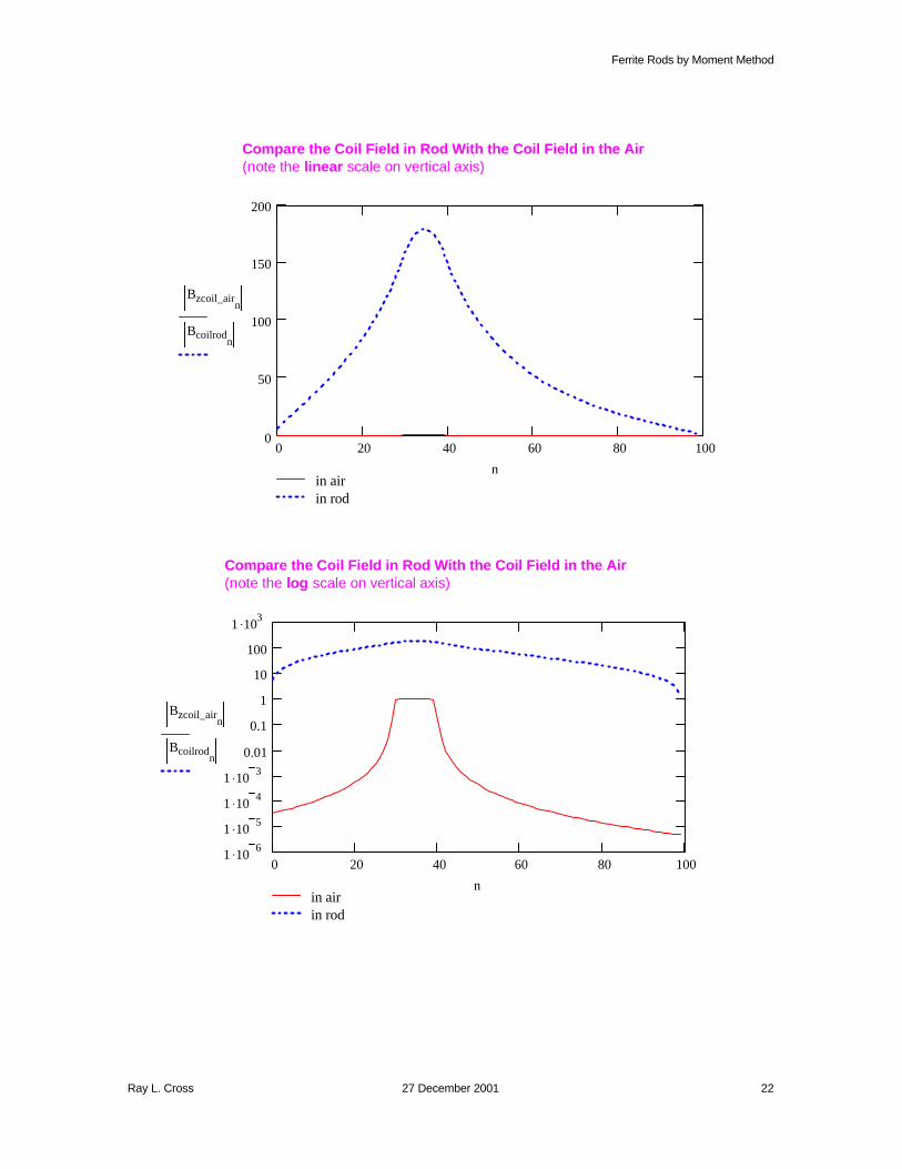
Compare the Coil Field in Rod With the Coil Field in the Air(note the linear scale on vertical axis)

0 20 40 60 80 1000

50

100

150

200

in air in rod

Bzcoil_airn

Bcoilrodn

n

Compare the Coil Field in Rod With the Coil Field in the Air(note the log scale on vertical axis)

0 20 40 60 80 1001 .10

6

1 .105

1 .104

1 .103

0.01

0.1

1

10

100

1 .103

in air in rod

Bzcoil_airn

Bcoilrodn

n



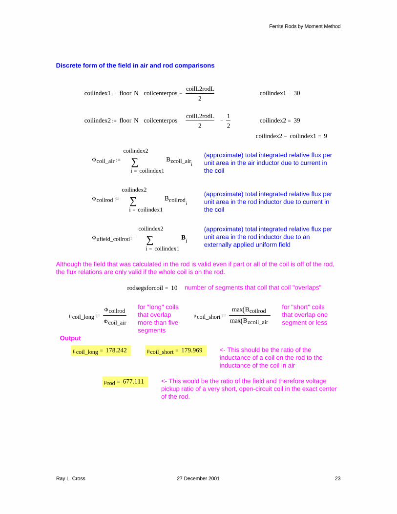
<- This would be the ratio of the field and therefore voltage pickup ratio of a very short, open-circuit coil in the exact center of the rod.

µrod 677.111=

<- This should be the ratio of the inductance of a coil on the rod to the inductance of the coil in air

µcoil_short 179.969=µcoil_long 178.242=

Output

µcoil_shortmax Bcoilrod( )

max Bzcoil_air( ):=µcoil_long

Φcoilrod

Φcoil_air:=

for "short" coils that overlap one segment or less

for "long" coils that overlap more than five segments

number of segments that coil that coil "overlaps"rodsegsforcoil 10=

Although the field that was calculated in the rod is valid even if part or all of the coil is off of the rod, the flux relations are only valid if the whole coil is on the rod.

Φufield_coilrod

coilindex1

coilindex2

i

Bi∑=

:=

(approximate) total integrated relative flux per unit area in the rod inductor due to an externally applied uniform field

Φcoilrod

coilindex1

coilindex2

i

Bcoilrodi∑

=

:=(approximate) total integrated relative flux per unit area in the rod inductor due to current in the coil

Φcoil_air

coilindex1

coilindex2

i

Bzcoil_airi∑

=

:=(approximate) total integrated relative flux per unit area in the air inductor due to current in the coil

coilindex2 coilindex1− 9=

coilindex2 39=coilindex2 floor N coilcenterposcoilL2rodL

2+

⋅1

2−

:=

coilindex1 30=coilindex1 floor N coilcenterposcoilL2rodL

2−

⋅

:=

Discrete form of the field in air and rod comparisons



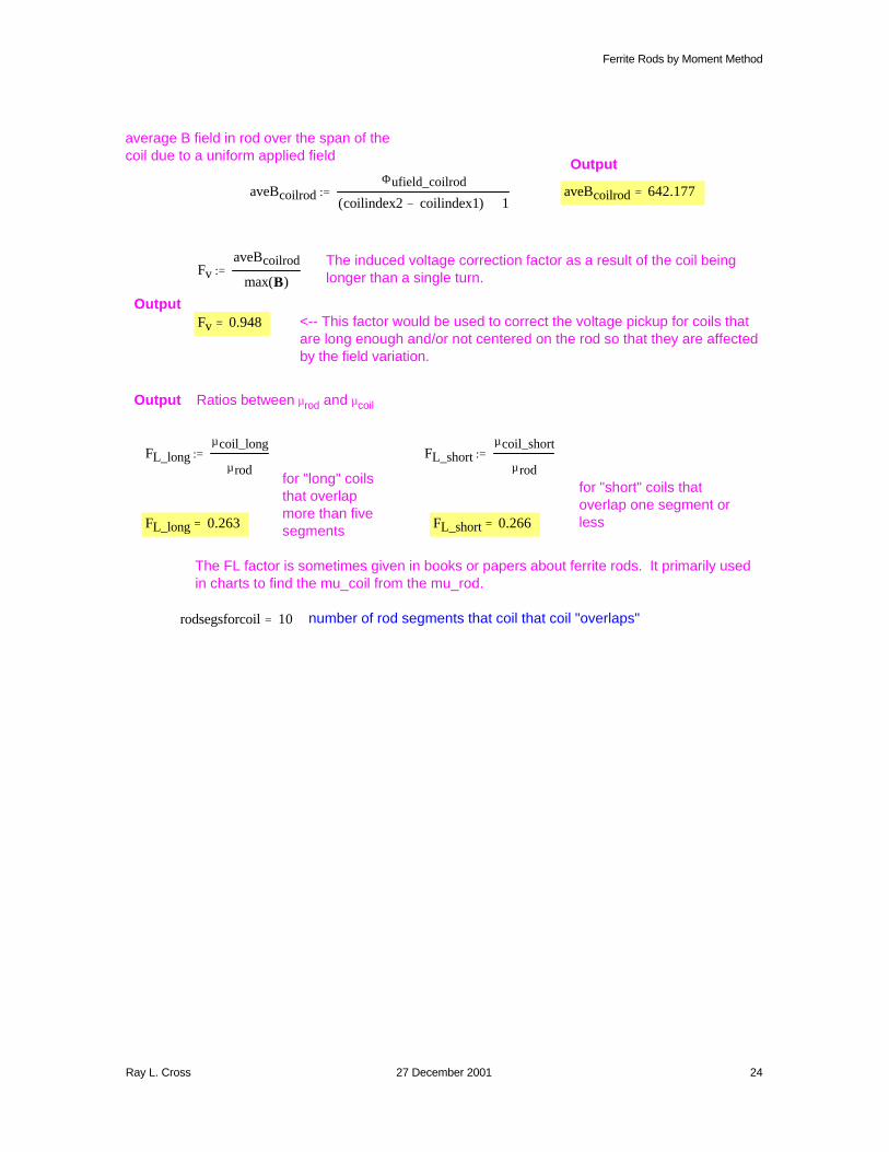
number of rod segments that coil that coil "overlaps"rodsegsforcoil 10=

The FL factor is sometimes given in books or papers about ferrite rods. It primarily used in charts to find the mu_coil from the mu_rod.

FL_short 0.266=FL_long 0.263=

for "short" coils that overlap one segment or less

for "long" coils that overlap more than five segments

FL_shortµcoil_short

µrod:=FL_long

µcoil_long

µrod:=

Output Ratios between µrod and µcoil

<-- This factor would be used to correct the voltage pickup for coils that are long enough and/or not centered on the rod so that they are affected by the field variation.

Fv 0.948=

Output

FvaveBcoilrod

max B( ):=

The induced voltage correction factor as a result of the coil being longer than a single turn.

aveBcoilrod 642.177=aveBcoilrodΦufield_coilrod

coilindex2 coilindex1−( ) 1+:=

Output

average B field in rod over the span of the coil due to a uniform applied field



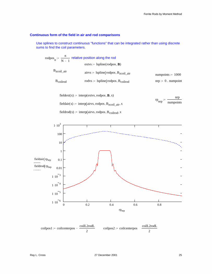
coilpos2 coilcenterposcoilL2rodL

2+:=coilpos1 coilcenterpos

coilL2rodL

2−:=

0 0.2 0.4 0.6 0.81 .10

6

1 .105

1 .10 4

1 .10 3

0.01

0.1

1

10

100

1 .103

fieldair rpnrp( )

fieldrod rpnrp( )

rpnrp

fieldrod x( ) interp airvs rodpos, Bcoilrod, x,( ):=

fieldair x( ) interp airvs rodpos, Bzcoil_air, x,( ):=rp

nrpnrp

numpoints:=

fieldext x( ) interp extvs rodpos, B, x,( ):=

nrp 0 numpoints..:=rodvs lspline rodpos Bcoilrod,( ):=Bcoilrod

numpoints 1000:=airvs lspline rodpos Bzcoil_air,( ):=

Bzcoil_air

extvs lspline rodpos B,( ):=

relative position along the rodrodposn

n

N 1−:=

Use splines to construct continuous "functions" that can be integrated rather than using discrete sums to find the coil parameters.

Continuous form of the field in air and rod comparisons



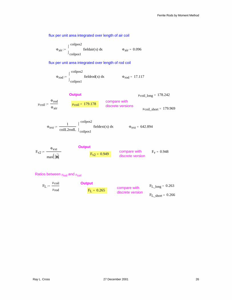
FL_short 0.266=FL 0.265=

compare with discrete version

FL_long 0.263=FLµcoil

µrod:=

Output

Ratios between µrod and µcoil

Fv2 0.949=Fv 0.948=compare with

discrete versionFv2

Φext

max B→( )

:=

Output

Φext 642.894=Φext1

coilL2rodL coilpos1

coilpos2

xfieldext x( )⌠⌡

d⋅:=

µcoil_short 179.969=µcoil 179.178=µcoil

Φrod

Φair:=

compare with discrete versions

µcoil_long 178.242=Output

Φrod 17.117=Φrodcoilpos1

coilpos2

xfieldrod x( )⌠⌡

d:=

flux per unit area integrated over length of rod coil

Φair 0.096=Φaircoilpos1

coilpos2

xfieldair x( )⌠⌡

d:=

flux per unit area integrated over length of air coil



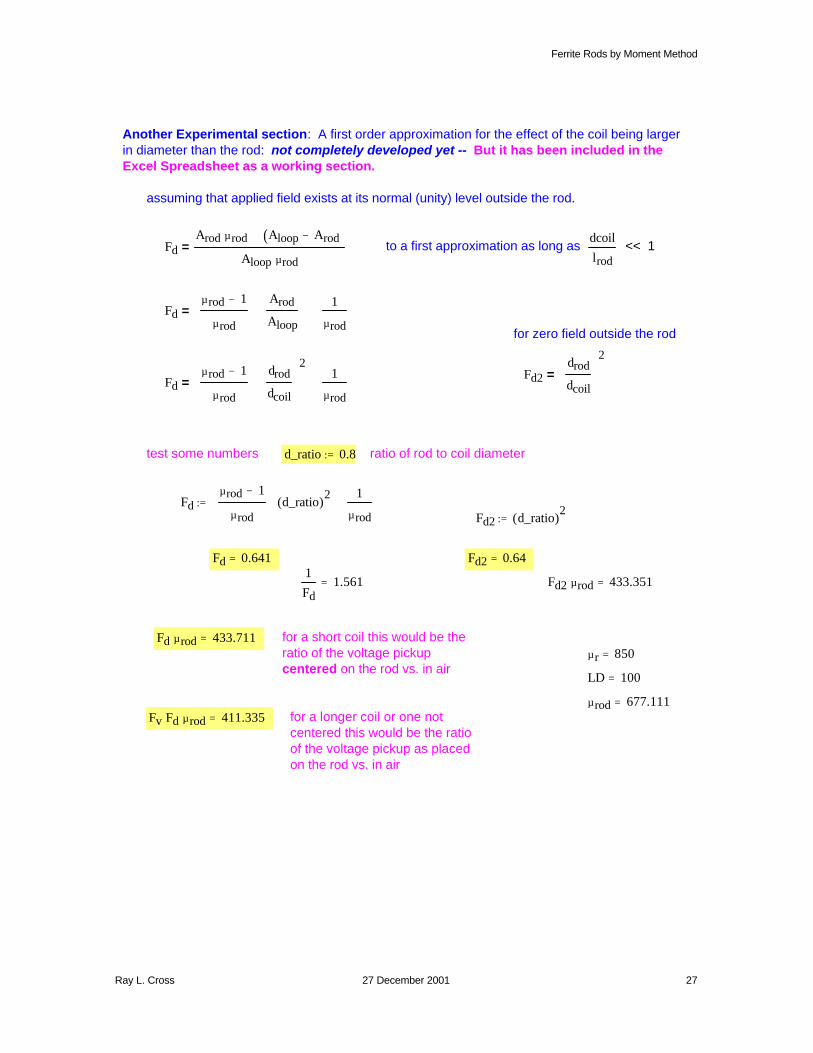
for a longer coil or one not centered this would be the ratio of the voltage pickup as placed on the rod vs. in air

Fv Fd⋅ µrod⋅ 411.335=µrod 677.111=

LD 100=

µr 850=

for a short coil this would be the ratio of the voltage pickup centered on the rod vs. in air

Fd µrod⋅ 433.711=

Fd2 µrod⋅ 433.351=1

Fd1.561=

Fd2 0.64=Fd 0.641=

Fd2 d_ratio( )2

:=Fd

µrod 1−

µrod

d_ratio( )2

⋅1

µrod+:=

ratio of rod to coil diameterd_ratio 0.8:=test some numbers

Fdµrod 1−

µrod

drod

dcoil

2

⋅1

µrod+=

Fd2drod

dcoil

2

=

for zero field outside the rod

Fdµrod 1−

µrod

Arod

Aloop

⋅1

µrod+=

<< 1dcoil

lrodto a first approximation as long asFd

Arod µrod⋅ Aloop Arod−( )+

Aloop µrod⋅=

assuming that applied field exists at its normal (unity) level outside the rod.

Another Experimental section: A first order approximation for the effect of the coil being larger in diameter than the rod: not completely developed yet -- But it has been included in the Excel Spreadsheet as a working section.



Hz1

2

a2

z2

a2

+( )⋅ I⋅ exp i− β⋅ z

2a2

+⋅( )⋅ i β⋅1

z2

a2

+

+

⋅=

Hz2 π⋅ a⋅( ) a⋅

r

I

4 π⋅ r⋅e

j− β⋅ r⋅⋅ j β⋅

1

r+

⋅

⋅=

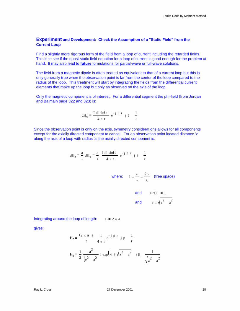
gives:

L 2 π⋅ a⋅=Integrating around the loop of length:

r z2

a2

+=and

sin θ( ) 1=and

(free space) βω

ν=

2 π⋅

λ=where:

dHza

rdHφ⋅=

a

r

I dl⋅ sin θ( )⋅

4 π⋅ r⋅e

j− β⋅ r⋅⋅ j β⋅

1

r+

⋅

⋅=

Since the observation point is only on the axis, symmetry considerations allows for all components except for the axially directed component to cancel. For an observation point located distance 'z' along the axis of a loop with radius 'a' the axially directed component is:

dHφI dl⋅ sin θ( )⋅

4 π⋅ r⋅e

j− β⋅ r⋅⋅ j β⋅

1

r+

⋅=

Experiment and Development: Check the Assumption of a "Static Field" from the Current Loop

Find a slightly more rigorous form of the field from a loop of current including the retarded fields. This is to see if the quasi-static field equation for a loop of current is good enough for the problem at hand. It may also lead to future formulations for partial-wave or full-wave solutions.

The field from a magnetic dipole is often treated as equivalent to that of a current loop but this is only generally true when the observation point is far from the center of the loop compared to the radius of the loop. This treatment will start by integrating the fields from the differential current elements that make up the loop but only as observed on the axis of the loop.

Only the magnetic component is of interest. For a differential segment the phi-field (from Jordan and Balmain page 322 and 323) is:



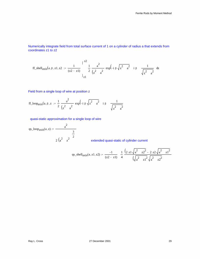
Numerically integrate field from total surface current of 1 on a cylinder of radius a that extends from coordinates z1 to z2

ff_shellaxis a β, z1, z2,( ) 1

z2 z1−( )

z1

z2

z1

2

a2

z2

a2

+( )⋅ exp i− β⋅ z

2a2

+⋅( )⋅ i β⋅1

z2

a2

+

+

⋅

⌠⌡

d⋅:=

Field from a single loop of wire at position z

ff_loopaxis a β, z,( ) 1

2

a2

z2

a2

+( )⋅ exp i− β⋅ z

2a2

+⋅( )⋅ i β⋅1

z2

a2

+

+

⋅:=

quasi-static approximation for a single loop of wire

qs_loopaxis a z,( )a2

2 a2

z2

+( )

3

2

⋅

:=

extended quasi-static of cylinder current

qs_shellaxis a z1, z2,( )1−

z2 z1−( )

1

4

2 z1⋅ a2

z22

+⋅ 2 z2⋅ a2

z12

+⋅−( )a2

z12

+ a2

z22

+⋅( )⋅

⋅:=



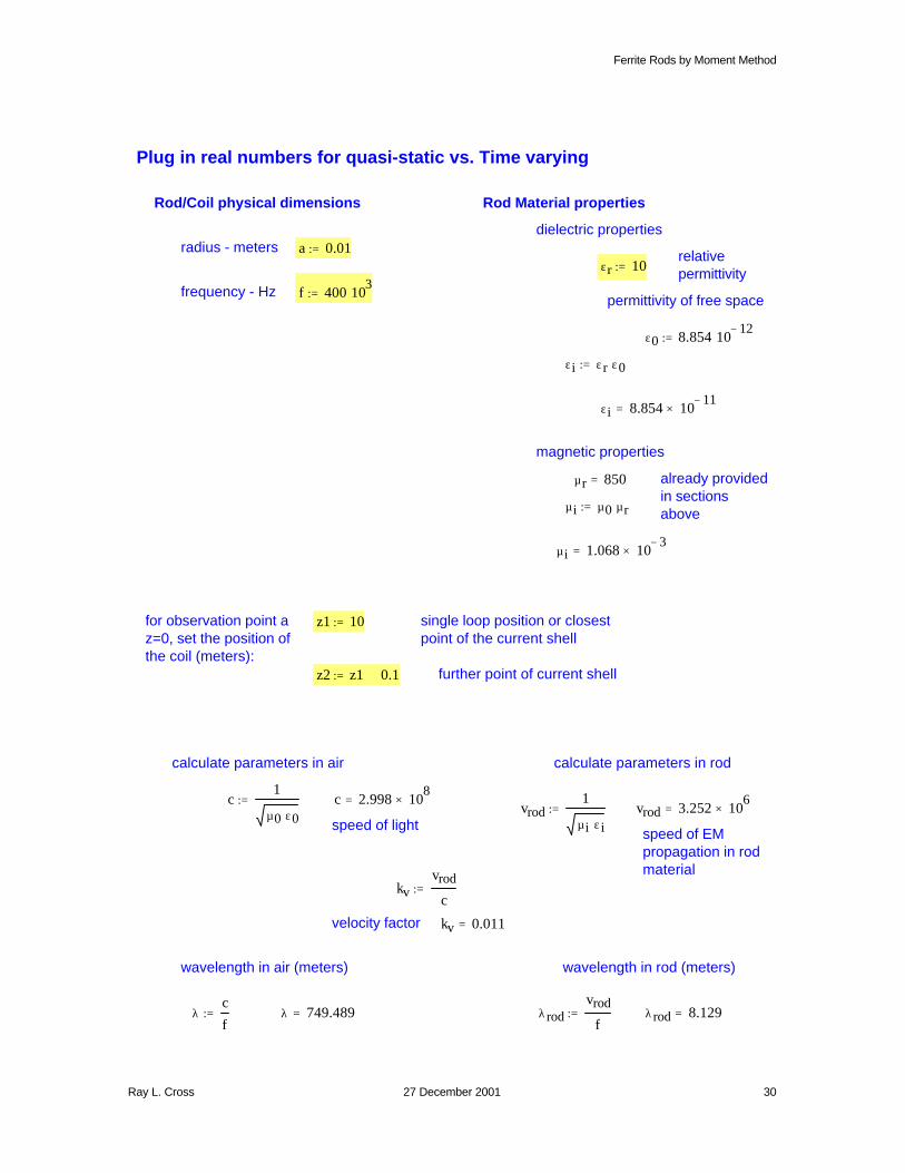
z1 10:= single loop position or closest point of the current shell

z2 z1 0.1+:= further point of current shell

calculate parameters in air calculate parameters in rod

c1

µ0 ε0⋅:= c 2.998 10

8×=

vrod1

µi ε i⋅:= vrod 3.252 10

6×=

speed of lightspeed of EM propagation in rod material

kvvrod

c:=

velocity factor kv 0.011=

wavelength in air (meters) wavelength in rod (meters)

λc

f:= λ 749.489= λrod

vrod

f:= λrod 8.129=

Plug in real numbers for quasi-static vs. Time varying

Rod/Coil physical dimensions Rod Material properties

dielectric propertiesradius - meters a 0.01:= relative

permittivityεr 10:=

frequency - Hz f 400 103

⋅:= permittivity of free space

ε0 8.854 1012−

⋅:=

εi ε r ε0⋅:=

εi 8.854 1011−

×=

magnetic properties

µr 850= already provided in sections aboveµi µ0 µr⋅:=

µi 1.068 103−

×=

for observation point a z=0, set the position of the coil (meters):



air_qs_loopaxis 5 108−

×=

arg rod_ff_loopaxis( ) 3.703− 103−

×=arg air_ff_loopaxis( ) 1.956− 10

4−×=

rod_ff_loopaxis 3.897 107−

×=air_ff_loopaxis 5.018 10

8−×=

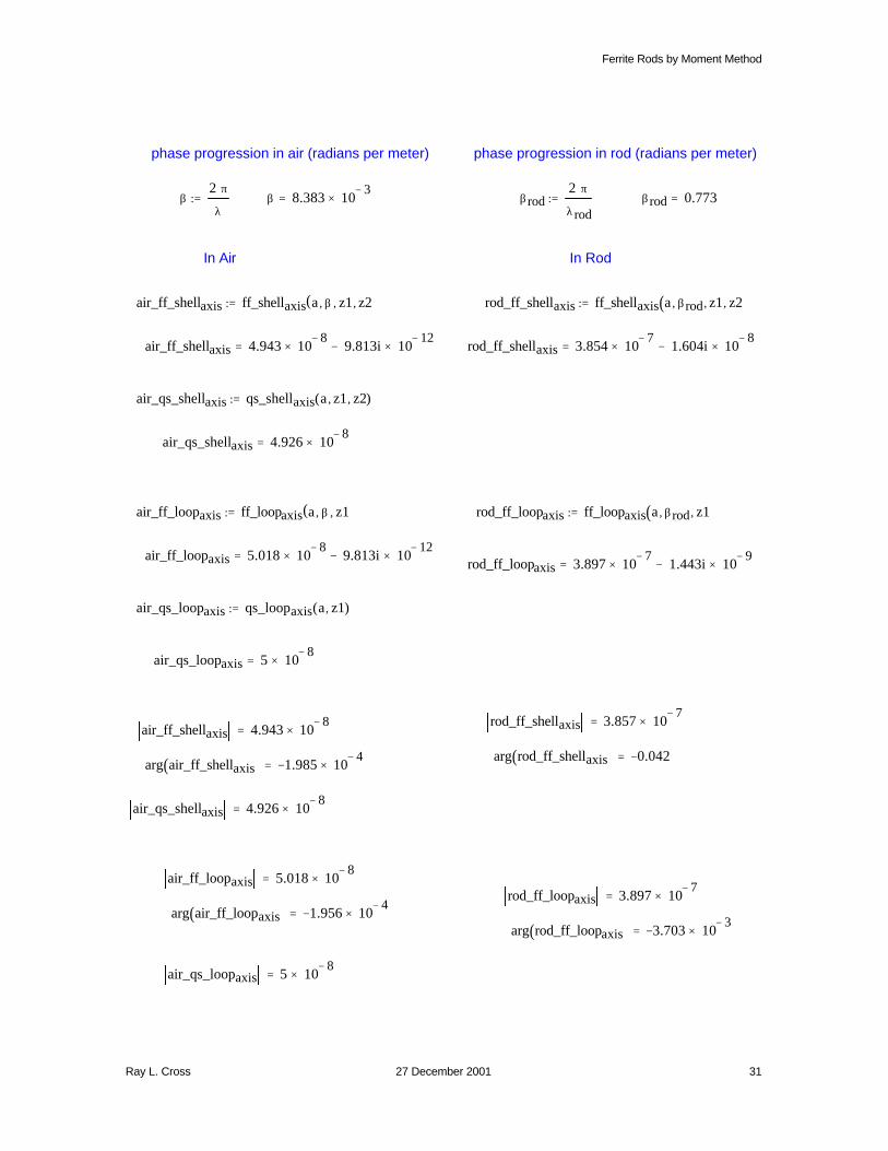
air_qs_shellaxis 4.926 108−

×=

arg air_ff_shellaxis( ) 1.985− 104−

×=arg rod_ff_shellaxis( ) 0.042−=

air_ff_shellaxis 4.943 108−

×=rod_ff_shellaxis 3.857 10

7−×=

air_qs_loopaxis 5 108−

×=

air_qs_loopaxis qs_loopaxis a z1,( ):=

rod_ff_loopaxis 3.897 107−

× 1.443i 109−

×−=air_ff_loopaxis 5.018 10

8−× 9.813i 10

12−×−=

rod_ff_loopaxis ff_loopaxis a βrod, z1,( ):=air_ff_loopaxis ff_loopaxis a β, z1,( ):=

air_qs_shellaxis 4.926 108−

×=

air_qs_shellaxis qs_shellaxis a z1, z2,( ):=

rod_ff_shellaxis 3.854 107−

× 1.604i 108−

×−=air_ff_shellaxis 4.943 108−

× 9.813i 1012−

×−=

rod_ff_shellaxis ff_shellaxis a βrod, z1, z2,( ):=air_ff_shellaxis ff_shellaxis a β, z1, z2,( ):=

In RodIn Air

βrod 0.773=βrod2 π⋅

λrod:=β 8.383 10

3−×=β

2 π⋅

λ:=

phase progression in rod (radians per meter)phase progression in air (radians per meter)



References and Bibliography:

[1] John Reed, "Ferrite Loops - Part II", The Lowdown, February 1999, p25-28

[2] Henry Jasik, Richard C. Johnson, Antenna Engineering Handbook, Third Edition, Georgia Institute of Technology, Atlanta, Georgia, 1993.

[3] E.C. Snelling, Soft Ferrites, Properties and Applications, Second Edition, Butterworth & Co (Great Britain) 1988.

[4] Richard Bozorth, Ferromagnetism, D. Van Nostrand Company, Inc. New York, 1951

[5] Bozorth and Chapin, "Demagnetizing Factors of Rods", Journal of Applied Physics, Volume 13, May 1942, pp. 320-326

[6] W.J. Polydoroff, High Frequency Magnetic Materials, John Wiley & Sons, New York, 1960

[7] G.G. Skitek, S.V. Marshall, Electromagnetic Concepts and Applications, Prentice-Hall, New Jersey 1982

[8] Robert Plonsey, Robert E. Collin, Principles and Applications of Electromagnetic Fields, McGraw-Hill, New York, 1961

[9] A.T. Adams, Electromagnetics for Engineers, Ronald Press, New York, 1971

[10] J.A. Stratton, Electromagnetic Theory, McGraw-Hill, 1941

[11] Constantine Balanis, Advanced Engineering Electromagnetics, John Wiley and Sons, New York, 1989

[12] Roger F. Harrington, Field Computation by Moment Methods, Robert E. Krieger Publishing Co. Malabar, Florida, 1968, 1982.

[*] Pettengill, Garland, and Meindl, "Receiving Antenna Design Miniature Receivers", IEEE Transactions on Antennas and Propagation, July 1988, p528-530

[*] DeVore and Bohley, "The Electrically Small Magnetically Loaded Multiturn Loop Antenna", IEEE Transactions on Antennas and Propagation, July 1977, p496-505

[**] Lo and Lee, Antenna Handbook, Van Nostrand Reinhold, New York, 1993, p6-20

[**] Jordan and Balmain, Electromagnetic Waves and Radiating Systems, 2nd Edition, Prentice Hall, Englewood Cliffs, New Jersey, 1968.


Documents

Some Magnetic Field Properties of Ferrite Rods … · Some Magnetic Field Properties of Ferrite Rods Used for Small Ferrite Loaded Receiving Antennas Solved by the Moment Method--