Sound System DesignReference Manual

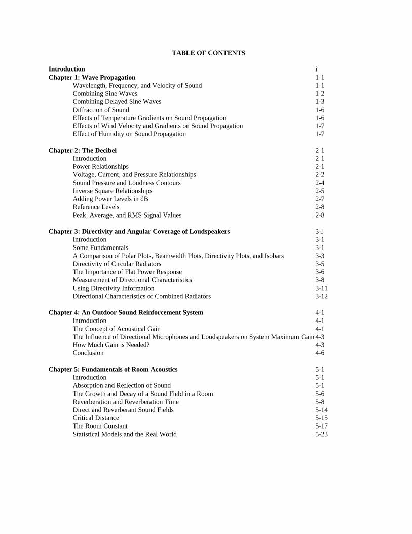
TABLE OF CONTENTS

Introduction iChapter 1: Wave Propagation 1-1

Wavelength, Frequency, and Velocity of Sound 1-1Combining Sine Waves 1-2Combining Delayed Sine Waves 1-3Diffraction of Sound 1-6Effects of Temperature Gradients on Sound Propagation 1-6Effects of Wind Velocity and Gradients on Sound Propagation 1-7Effect of Humidity on Sound Propagation 1-7

Chapter 2: The Decibel 2-1Introduction 2-1Power Relationships 2-1Voltage, Current, and Pressure Relationships 2-2Sound Pressure and Loudness Contours 2-4Inverse Square Relationships 2-5Adding Power Levels in dB 2-7Reference Levels 2-8Peak, Average, and RMS Signal Values 2-8

Chapter 3: Directivity and Angular Coverage of Loudspeakers 3-lIntroduction 3-1Some Fundamentals 3-1A Comparison of Polar Plots, Beamwidth Plots, Directivity Plots, and Isobars 3-3Directivity of Circular Radiators 3-5The Importance of Flat Power Response 3-6Measurement of Directional Characteristics 3-8Using Directivity Information 3-11Directional Characteristics of Combined Radiators 3-12

Chapter 4: An Outdoor Sound Reinforcement System 4-1Introduction 4-1The Concept of Acoustical Gain 4-1The Influence of Directional Microphones and Loudspeakers on System Maximum Gain 4-3How Much Gain is Needed? 4-3Conclusion 4-6

Chapter 5: Fundamentals of Room Acoustics 5-1Introduction 5-1Absorption and Reflection of Sound 5-1The Growth and Decay of a Sound Field in a Room 5-6Reverberation and Reverberation Time 5-8Direct and Reverberant Sound Fields 5-14Critical Distance 5-15The Room Constant 5-17Statistical Models and the Real World 5-23

Chapter 6: Behavior of Sound Systems Indoors 6-1 Introduction 6-1 Acoustical Feedback and Potential System Gain 6-1 Sound Field Calculations for a Small Room 6-2 Calculations for a Medium-size Room 6-5 Calculations for a Distributed Loudspeaker System 6-9 System Gain vs. Frequency Response 6-10 The Indoor Gain Equation 6-11 Measuring Sound System Gain 6-12 General Requirements for Speech Intelligibility 6-12 The Role of Time Delay in Sound Reinforcement 6-18 System Equalization and Power Response of Loudspeakers 6-19 System Design Overview 6-21

Chapter 7: System Architecture 7-1Introduction 7-1A Typical Signal Flow Diagram 7-1Specifying and Powering of Loudspeakers 7-3 Case Studies:A - Multi-channel Reinforcement System in a Theater 7-7B - Very-low-frequency (VLF) Augmentation: Sub-woofers 7-9C - Distributed System in a Large Church 7-11D - A 70-volt Distribution System 7-12E - Extending Power Ba.ndwidth 7-16

INTRODUCTION

JBL's Sound System Design Reference Manual is based largely on the Sound Workshop manualintroduced in 1976. That earlier work, prepared by George Augspurger, was the basis for a series ofsystem design seminars held at various cities in the United States, and its coverage of room acousticsand indoor sound system analysis was noted for its thorough and logical approach. Those sections aremaintained intact in the present work.

In addition, sections covering basic acoustics, the decibel, and loudspeaker directivity have beenexpanded, and system design and architecture have been given more detailed coverage. In general,greater emphasis has been given to specific JBL hardware, including the family of biradial horns, anddesign approaches based on the notion of flat power response have been stressed.

It may be a long time before we in the United States abandon feet, miles, and the like, for meters andkilometers in our everyday lives. There is no question however that metric, or SI as it is called today,has become the preferred system of units for scientific work. In an effort to be consistent, this documenthas been written with all examples in SI units. Design charts however have been given in both SI andEnglish units for the convenience of all users. It is of no small concern to us at JBL that more than halfof all our professional products are sold to foreign markets where the metric system has long beenstandard, and it is our intention that this document be of just as much use in those countries as in theUnited States.

The technical competence of professional dealers and sound contractors is much higher today than itwas when the Sound Workshop manual was introduced over six years ago. It is JBL's feeling that theserious contractor or professional dealer of today is ready to move away from simply plugging numbersinto equations. Instead, he is eager to learn what the equations really mean, and he is intent on learninghow loudspeakers and rooms interact, however complex that may be. It is for the student with such anoutlook that this manual is intended.

John EargleMarch 1986=================================================================

While products, system strategies and design tools change and improve, the basic knowledge is stillrequired to implement good systems. This manual, that has been a benefit to so many, has beenscanned and reorganized for electronic distribution, with the hopes that is be useful to many more, overa much wider reach.

Jeffry LongNovember 1994

CHAPTER 1: WAVE PROPAGATION

Wavelength, Frequency, and Velocity of Sound

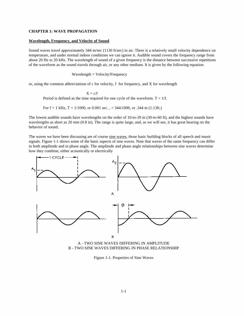
Sound waves travel approximately 344 m/sec (1130 ft/sec) in air. There is a relatively small velocity dependence ontemperature, and under normal indoor conditions we can ignore it. Audible sound covers the frequency range fromabout 20 Hz to 20 kHz. The wavelength of sound of a given frequency is the distance between successive repetitionsof the waveform as the sound travels through air, or any other medium. It is given by the following equation

Wavelength = Velocity/Frequency

or, using the common abbreviations of c for velocity, f for frequency, and X for wavelength

X = c/fPeriod is defined as the time required for one cycle of the waveform. T = 1/f.

For f = 1 kHz, T = 1/1000, or 0.001 sec. , = 344/1000, or .344 m (1.13ft.)

The lowest audible sounds have wavelengths on the order of 10-to-20 m (30-to-60 ft), and the highest sounds havewavelengths as short as 20 mm (0.8 in). The range is quite large, and, as we will see, it has great bearing on thebehavior of sound.

The waves we have been discussing are of course sine waves, those basic building blocks of all speech and musicsignals. Figure 1-1 shows some of the basic aspects of sine waves. Note that waves of the same frequency can differin both amplitude and in phase angle. The amplitude and phase angle relationships between sine waves determinehow they combine, either acoustically or electrically

A - TWO SINE WAVES DIFFERING IN AMPLITUDEB - TWO SINE WAVES DIFFERING IN PHASE RELATIONSHIP

Figure 1-1. Properties of Sine Waves

1-1

Combining Sine Waves

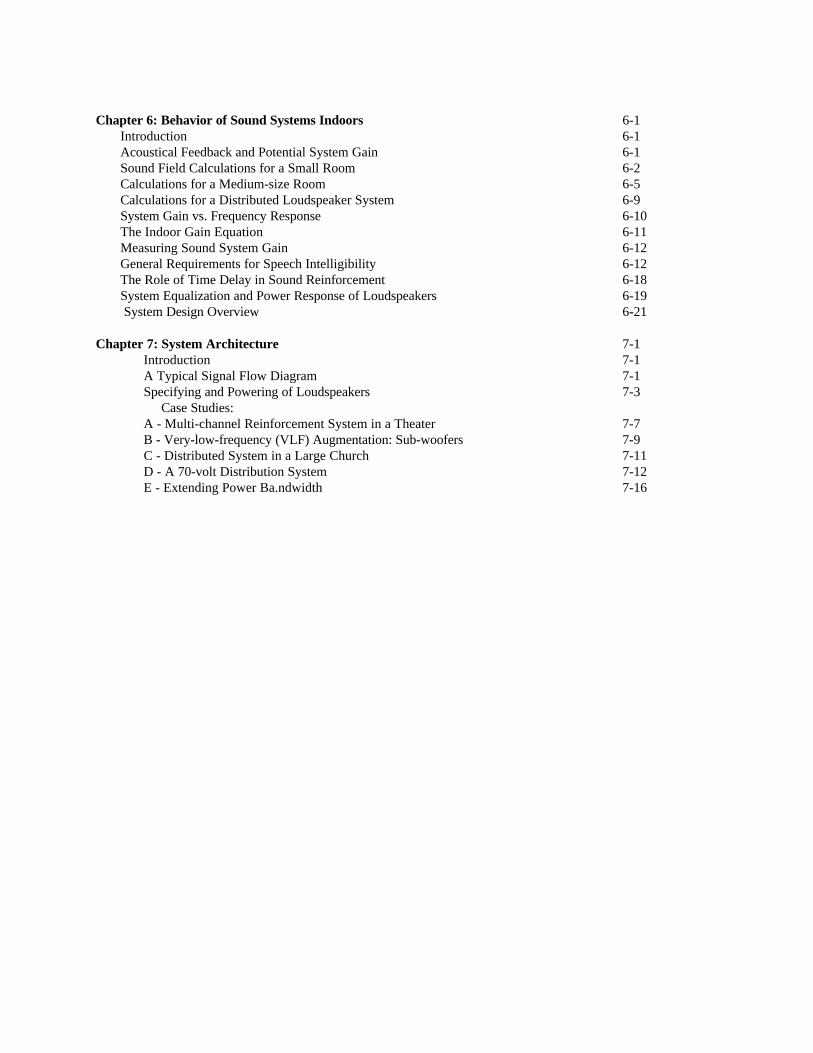
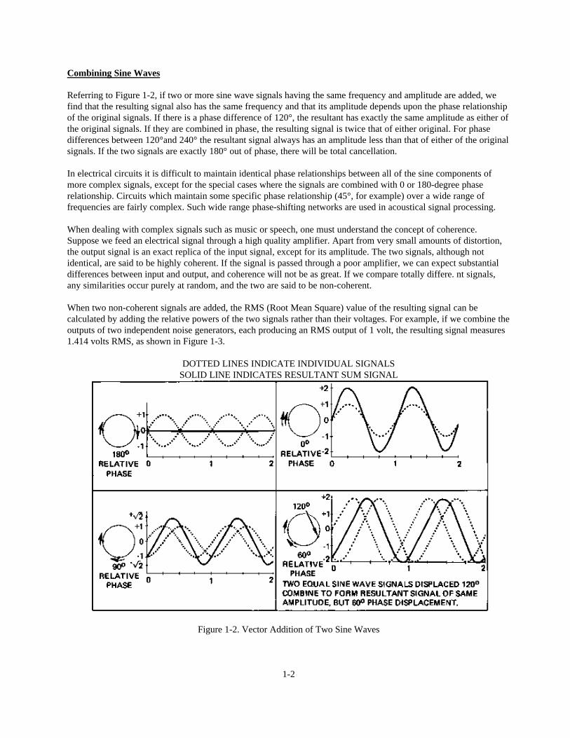
Referring to Figure 1-2, if two or more sine wave signals having the same frequency and amplitude are added, wefind that the resulting signal also has the same frequency and that its amplitude depends upon the phase relationshipof the original signals. If there is a phase difference of 120°, the resultant has exactly the same amplitude as either ofthe original signals. If they are combined in phase, the resulting signal is twice that of either original. For phasedifferences between 120°and 240° the resultant signal always has an amplitude less than that of either of the originalsignals. If the two signals are exactly 180° out of phase, there will be total cancellation.

In electrical circuits it is difficult to maintain identical phase relationships between all of the sine components ofmore complex signals, except for the special cases where the signals are combined with 0 or 180-degree phaserelationship. Circuits which maintain some specific phase relationship (45°, for example) over a wide range offrequencies are fairly complex. Such wide range phase-shifting networks are used in acoustical signal processing.

When dealing with complex signals such as music or speech, one must understand the concept of coherence.Suppose we feed an electrical signal through a high quality amplifier. Apart from very small amounts of distortion,the output signal is an exact replica of the input signal, except for its amplitude. The two signals, although notidentical, are said to be highly coherent. If the signal is passed through a poor amplifier, we can expect substantialdifferences between input and output, and coherence will not be as great. If we compare totally differe. nt signals,any similarities occur purely at random, and the two are said to be non-coherent.

When two non-coherent signals are added, the RMS (Root Mean Square) value of the resulting signal can becalculated by adding the relative powers of the two signals rather than their voltages. For example, if we combine theoutputs of two independent noise generators, each producing an RMS output of 1 volt, the resulting signal measures1.414 volts RMS, as shown in Figure 1-3.

DOTTED LINES INDICATE INDIVIDUAL SIGNALSSOLID LINE INDICATES RESULTANT SUM SIGNAL

Figure 1-2. Vector Addition of Two Sine Waves

1-2

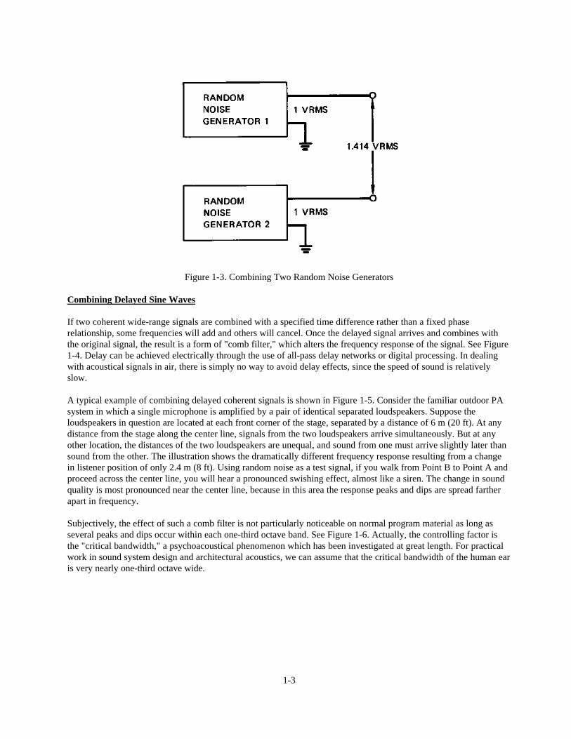
Figure 1-3. Combining Two Random Noise Generators

Combining Delayed Sine Waves

If two coherent wide-range signals are combined with a specified time difference rather than a fixed phaserelationship, some frequencies will add and others will cancel. Once the delayed signal arrives and combines withthe original signal, the result is a form of "comb filter," which alters the frequency response of the signal. See Figure1-4. Delay can be achieved electrically through the use of all-pass delay networks or digital processing. In dealingwith acoustical signals in air, there is simply no way to avoid delay effects, since the speed of sound is relativelyslow.

A typical example of combining delayed coherent signals is shown in Figure 1-5. Consider the familiar outdoor PAsystem in which a single microphone is amplified by a pair of identical separated loudspeakers. Suppose theloudspeakers in question are located at each front corner of the stage, separated by a distance of 6 m (20 ft). At anydistance from the stage along the center line, signals from the two loudspeakers arrive simultaneously. But at anyother location, the distances of the two loudspeakers are unequal, and sound from one must arrive slightly later thansound from the other. The illustration shows the dramatically different frequency response resulting from a changein listener position of only 2.4 m (8 ft). Using random noise as a test signal, if you walk from Point B to Point A andproceed across the center line, you will hear a pronounced swishing effect, almost like a siren. The change in soundquality is most pronounced near the center line, because in this area the response peaks and dips are spread fartherapart in frequency.

Subjectively, the effect of such a comb filter is not particularly noticeable on normal program material as long asseveral peaks and dips occur within each one-third octave band. See Figure 1-6. Actually, the controlling factor isthe "critical bandwidth," a psychoacoustical phenomenon which has been investigated at great length. For practicalwork in sound system design and architectural acoustics, we can assume that the critical bandwidth of the human earis very nearly one-third octave wide.

1-3

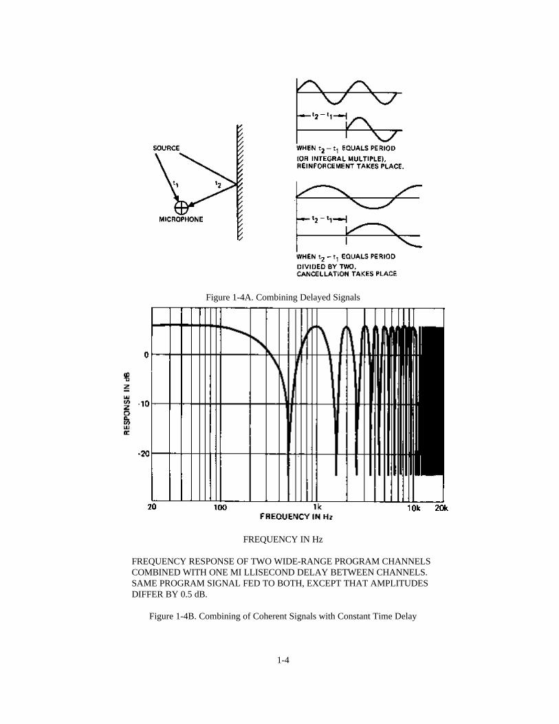
Figure 1-4A. Combining Delayed Signals

FREQUENCY IN Hz

FREQUENCY RESPONSE OF TWO WIDE-RANGE PROGRAM CHANNELSCOMBINED WITH ONE MI LLISECOND DELAY BETWEEN CHANNELS.SAME PROGRAM SIGNAL FED TO BOTH, EXCEPT THAT AMPLITUDESDIFFER BY 0.5 dB.

Figure 1-4B. Combining of Coherent Signals with Constant Time Delay

1-4

In houses of worship, the system should be suspended high overhead and centered. In spaces which do not haveconsiderable height, there is a strong temptation to use two loudspeakers, one on either side of the platform, feedingboth the same program. We DO NOT recommend this. Figure 4 shows what happens withsplit systems for listeners who are displaced from the center line by just a small amount.

FIGURE 4. GENERATION OF INTERFERENCE EFFECTS (COMB FILTER RESPONSE) BY A SPLIT ARRAY.

FREQUENCY HzInterference Effects from Two Separated Loudspeakers Producing Coherent Signals

1/3 OCTAVE CENTER FREQUENCY 1N HzSOLID LINE MEASURED SINE WAVE FREQUENCY RESPONSE.DOTTED LINE 1/3 OCTAVE BAND RESPONSE, CLOSELY CORRESPONDING TO

SUBJECTIVE TONAL QUALITY WHEN LISTENING TO NORMALPROGRAM MATERIAL. ABOVE 1 kHz SUBJECTIVE RESPONSE ISESSENTIALLY FLAT.

Subjective Effect of Comb Filter Response

1-5

Diffraction of Sound

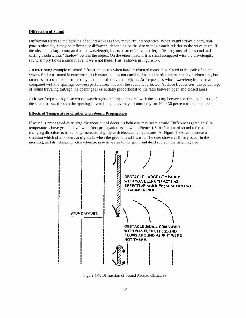
Diffraction refers to the bending of sound waves as they move around obstacles. When sound strikes a hard, non-porous obstacle, it may be reflected or diffracted, depending on the size of the obstacle relative to the wavelength. Ifthe obstacle is large compared to the wavelength, it acts as an effective barrier, reflecting most of the sound andcasting a substantial "shadow" behind the object. On the other hand, if it is small compared with the wavelength,sound simply flows around it as if it were not there. This is shown in Figure 1-7.

An interesting example of sound diffraction occurs when hard, perforated material is placed in the path of soundwaves. So far as sound is concerned, such material does not consist of a solid barrier interrupted by perforations, butrather as an open area obstructed by a number of individual objects. At frequencies whose wavelengths are smallcompared with the spacings between perforations, most of the sound is reflected. At these frequencies, the percentageof sound traveling thr6ugh the openings is essentially proportional to the ratio between open and closed areas.

At lower frequencies (those whose wavelengths are large compared with the spacing between perforations), most ofthe sound passes through the openings, even though they may account only for 20 or 30 percent of the total area.

Effects of Temperature Gradients on Sound Propagation

If sound is propagated over large distances out of doors, its behavior may seem erratic. Differences (gradients) intemperature above ground level will affect propagation as shown in Figure 1-8. Refraction of sound refers to itschanging direction as its velocity increases slightly with elevated temperatures. At Figure 1-8A, we observe asituation which often occurs at nightfall, when the ground is still warm. The case shown at B may occur in themorning, and its "skipping" characteristic may give rise to hot spots and dead spots in the listening area.

Figure 1-7. Diffraction of Sound Around Obstacles

1-6

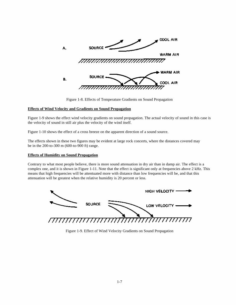
Figure 1-8. Effects of Temperature Gradients on Sound Propagation

Effects of Wind Velocity and Gradients on Sound Propagation

Figure 1-9 shows the effect wind velocity gradients on sound propagation. The actual velocity of sound in this case isthe velocity of sound in still air plus the velocity of the wind itself.

Figure 1-10 shows the effect of a cross breeze on the apparent direction of a sound source.

The effects shown in these two figures may be evident at large rock concerts, where the distances covered maybe in the 200-to-300 m (600-to-900 ft) range.

Effects of Humidity on Sound Propagation

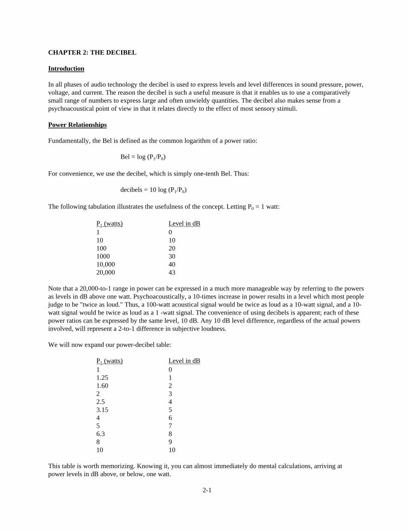
Contrary to what most people believe, there is more sound attenuation in dry air than in damp air. The effect is acomplex one, and it is shown in Figure 1-11. Note that the effect is significant only at frequencies above 2 kHz. Thismeans that high frequencies will be attentuated more with distance than low frequencies will be, and that thisattenuation will be greatest when the relative humidity is 20 percent or less.

Figure 1-9. Effect of Wind Velocity Gradients on Sound Propagation

1-7

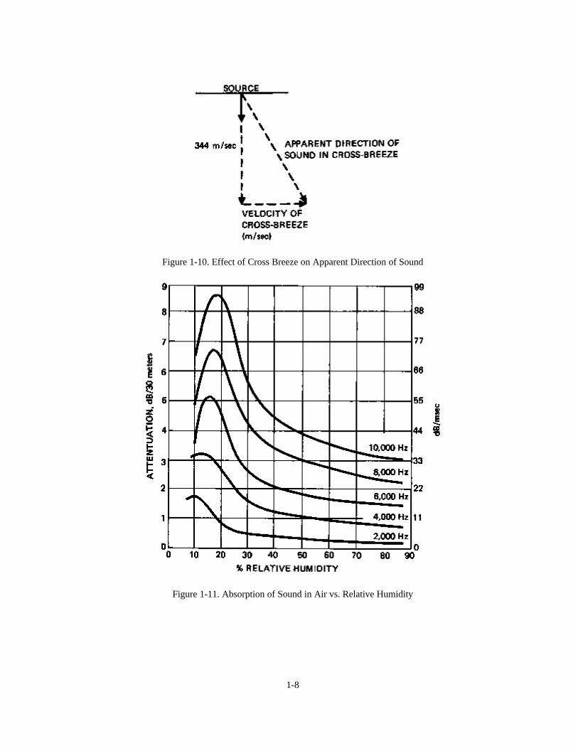
Figure 1-10. Effect of Cross Breeze on Apparent Direction of Sound

Figure 1-11. Absorption of Sound in Air vs. Relative Humidity

1-8

CHAPTER 2: THE DECIBEL

Introduction

In all phases of audio technology the decibel is used to express levels and level differences in sound pressure, power,voltage, and current. The reason the decibel is such a useful measure is that it enables us to use a comparativelysmall range of numbers to express large and often unwieldy quantities. The decibel also makes sense from apsychoacoustical point of view in that it relates directly to the effect of most sensory stimuli.

Power Relationships

Fundamentally, the Bel is defined as the common logarithm of a power ratio:

Bel = log (P1/P0)

For convenience, we use the decibel, which is simply one-tenth Bel. Thus:

decibels = 10 log (P1/P0)

The following tabulation illustrates the usefulness of the concept. Letting P0 = 1 watt:

P1 (watts) Level in dB1 010 10100 201000 3010,000 4020,000 43

Note that a 20,000-to-1 range in power can be expressed in a much more manageable way by referring to the powersas levels in dB above one watt. Psychoacoustically, a 10-times increase in power results in a level which most peoplejudge to be "twice as loud." Thus, a 100-watt acoustical signal would be twice as loud as a 10-watt signal, and a 10-watt signal would be twice as loud as a 1 -watt signal. The convenience of using decibels is apparent; each of thesepower ratios can be expressed by the same level, 10 dB. Any 10 dB level difference, regardless of the actual powersinvolved, will represent a 2-to-1 difference in subjective loudness.

We will now expand our power-decibel table:

P1 (watts) Level in dB1 01.25 11.60 22 32.5 43.15 54 65 76.3 88 910 10

This table is worth memorizing. Knowing it, you can almost immediately do mental calculations, arriving atpower levels in dB above, or below, one watt.

2-1

Here are some examples:

1. What power level is represented by 80 watts? First, locate 8 watts in the left column and note that thecorresponding level is 9 dB. Then, note that 80 is 10 times 8, giving another 10 dB. Thus, 9 + 10 = 19 dB.

2. What power level is represented by 1 milliwatt? 0.1 watt represents a level of minus 10 dB. 0.01 represents a level10 dB lower, and finally 0.001 represents an additional level decrease of 10 dB. Thus, -10 - 10 - 10 = -30 dB.

3. What power level is represented by 4 mill iwatts? As we have seen, the power level of 1 milliwatt is = 30 dB. 2milliwatts represents a level increase of 3 dB, and from 2 to 4 milliwatts there is an additional 3 dB level increase.Thus, -30 + 3 + 3 = -24 dB.

4. What is the level difference between 40 and 100 watts? Note from the table that the level corresponding to 4 wattsis 6 dB, and the level corresponding to 10 watts is 10 dB, a difference of 4 dB. Since the level of 40 watts is 10 dBgreater than for 4 watts, and the level of 80 watts is 10 dB greater than for 8 watts, we have: 6 - 10 + 10 -10 = 4 dB.

We have done this example the long way, just to show the rigorous approach. However, we could simply havestopped with our first observation, noting that the dB level difference between 4 and 10 watts, .4 and 1 watt, or 400and 1000 watts will always be the same, 4 dB, because they all represent the same power ratio.

The level difference in dB can be converted back to a power ratio by means of the following equation:

Power ratio = 10 dB/10

For example, find the power ratio of a level difference of 13 dB:

Power ratio = 1013/10 = 101.3 = 20.

The reader should gain a reasonable skill in dealing with power ratios expressed as level differences in dB. A good"feel" for decibels is a qualification for any audio engineer or sound contractor. An extended nomograph forconverting power ratios to level differences in dB is given in Figure 2-1.

Voltage, Current, and Pressure Relationships

The decibel fundamentally relates to power ratios, and we can use voltage, current, and pressure ratios as they relateto power. Electrical power can be represented as:

P= EIP = I2ZP = E2/Z

Because power is proportional to the square of the voltage, the effect of doubling the voltaxqe is to quadruple thepower: (2E)2/Z = 4(E)2/Z. As an example, let E = 1 Volt and Z = 1 ohm. Then, P = E2/Z = 1 watt.Now, let E = 2 volts; then, P = (2)2/1 = 4 watts.

The same holds true for current, and the following equations must be used to express power levels in dB usingvoltage and current ratios:

dB level = 10 log(E1/E0)2 = 20 log(E1/E0), and...

dB level = 10 log(I1/I0)2 = 20 log(I1/I0).

2-2

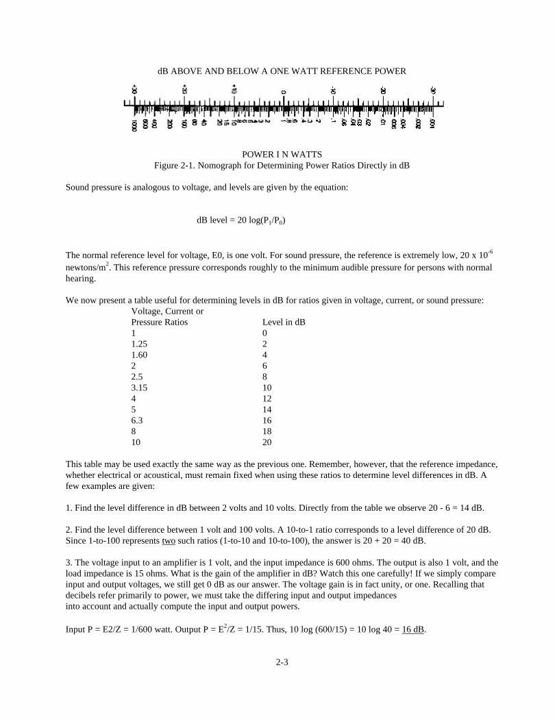
dB ABOVE AND BELOW A ONE WATT REFERENCE POWER

POWER I N WATTSFigure 2-1. Nomograph for Determining Power Ratios Directly in dB

Sound pressure is analogous to voltage, and levels are given by the equation:

dB level = 20 log(P1/P0)

The normal reference level for voltage, E0, is one volt. For sound pressure, the reference is extremely low, 20 x 10-6

newtons/m2. This reference pressure corresponds roughly to the minimum audible pressure for persons with normalhearing.

We now present a table useful for determining levels in dB for ratios given in voltage, current, or sound pressure:Voltage, Current orPressure Ratios Level in dB1 01.25 21.60 42 62.5 83.15 104 125 146.3 168 1810 20

This table may be used exactly the same way as the previous one. Remember, however, that the reference impedance,whether electrical or acoustical, must remain fixed when using these ratios to determine level differences in dB. Afew examples are given:

1. Find the level difference in dB between 2 volts and 10 volts. Directly from the table we observe 20 - 6 = 14 dB.

2. Find the level difference between 1 volt and 100 volts. A 10-to-1 ratio corresponds to a level difference of 20 dB.Since 1-to-100 represents two such ratios (1-to-10 and 10-to-100), the answer is 20 + 20 = 40 dB.

3. The voltage input to an amplifier is 1 volt, and the input impedance is 600 ohms. The output is also 1 volt, and theload impedance is 15 ohms. What is the gain of the amplifier in dB? Watch this one carefully! If we simply compareinput and output voltages, we still get 0 dB as our answer. The voltage gain is in fact unity, or one. Recalling thatdecibels refer primarily to power, we must take the differing input and output impedancesinto account and actually compute the input and output powers.

Input P = E2/Z = 1/600 watt. Output P = E2/Z = 1/15. Thus, 10 log (600/15) = 10 log 40 = 16 dB.

2-3

The level difference in dB can be converted back to a voltage, current, or pressure ratio by means of the followingequation:

Ratio = 10 dB/20

For example, find the voltage ratio of a level difference of 66 dB:

Voltage Ratio = 10 66/20 = 10 3.3 = 2000.

Sound Pressure and Loudness Contours

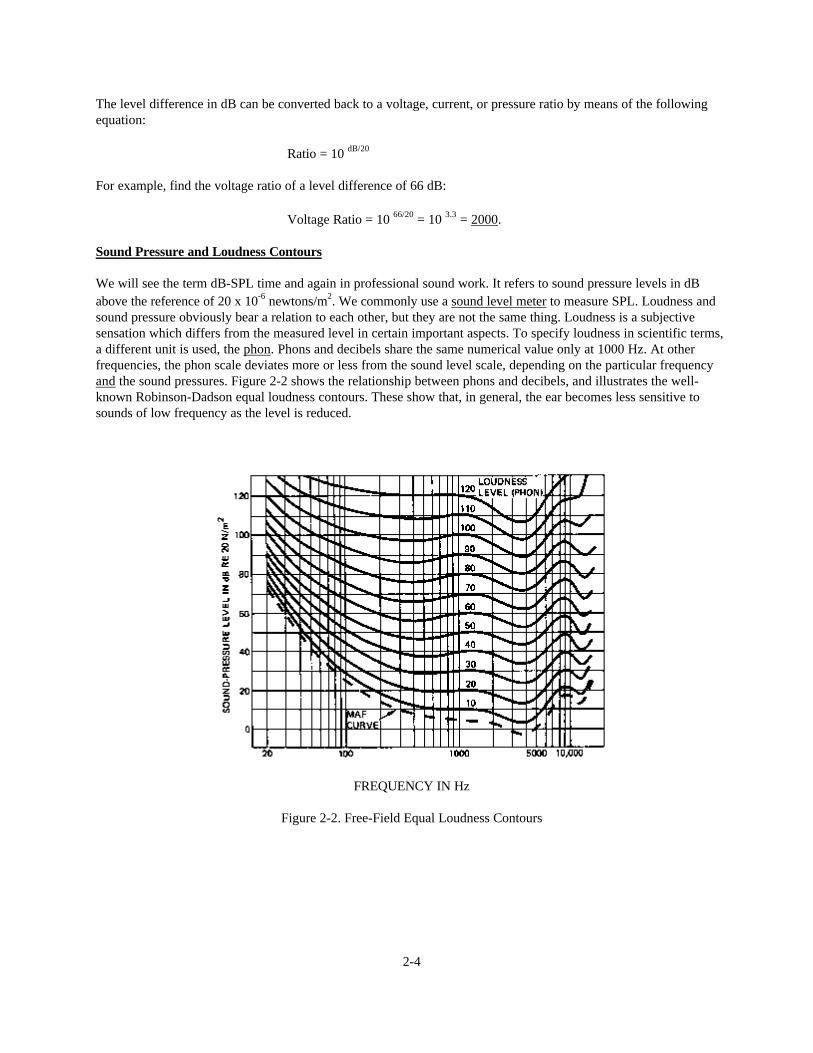
We will see the term dB-SPL time and again in professional sound work. It refers to sound pressure levels in dBabove the reference of 20 x 10-6 newtons/m2. We commonly use a sound level meter to measure SPL. Loudness andsound pressure obviously bear a relation to each other, but they are not the same thing. Loudness is a subjectivesensation which differs from the measured level in certain important aspects. To specify loudness in scientific terms,a different unit is used, the phon. Phons and decibels share the same numerical value only at 1000 Hz. At otherfrequencies, the phon scale deviates more or less from the sound level scale, depending on the particular frequencyand the sound pressures. Figure 2-2 shows the relationship between phons and decibels, and illustrates the well-known Robinson-Dadson equal loudness contours. These show that, in general, the ear becomes less sensitive tosounds of low frequency as the level is reduced.

FREQUENCY IN Hz

Figure 2-2. Free-Field Equal Loudness Contours

2-4

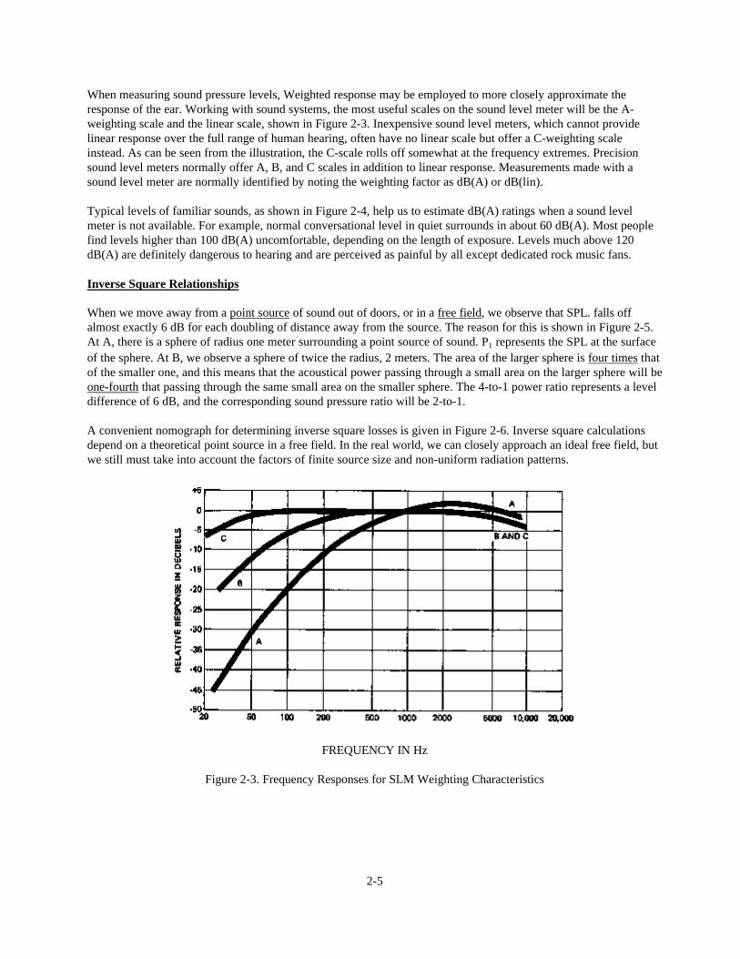
When measuring sound pressure levels, Weighted response may be employed to more closely approximate theresponse of the ear. Working with sound systems, the most useful scales on the sound level meter will be the A-weighting scale and the linear scale, shown in Figure 2-3. Inexpensive sound level meters, which cannot providelinear response over the full range of human hearing, often have no linear scale but offer a C-weighting scaleinstead. As can be seen from the illustration, the C-scale rolls off somewhat at the frequency extremes. Precisionsound level meters normally offer A, B, and C scales in addition to linear response. Measurements made with asound level meter are normally identified by noting the weighting factor as dB(A) or dB(lin).

Typical levels of familiar sounds, as shown in Figure 2-4, help us to estimate dB(A) ratings when a sound levelmeter is not available. For example, normal conversational level in quiet surrounds in about 60 dB(A). Most peoplefind levels higher than 100 dB(A) uncomfortable, depending on the length of exposure. Levels much above 120dB(A) are definitely dangerous to hearing and are perceived as painful by all except dedicated rock music fans.

Inverse Square Relationships

When we move away from a point source of sound out of doors, or in a free field, we observe that SPL. falls offalmost exactly 6 dB for each doubling of distance away from the source. The reason for this is shown in Figure 2-5.At A, there is a sphere of radius one meter surrounding a point source of sound. P1 represents the SPL at the surfaceof the sphere. At B, we observe a sphere of twice the radius, 2 meters. The area of the larger sphere is four times thatof the smaller one, and this means that the acoustical power passing through a small area on the larger sphere will beone-fourth that passing through the same small area on the smaller sphere. The 4-to-1 power ratio represents a leveldifference of 6 dB, and the corresponding sound pressure ratio will be 2-to-1.

A convenient nomograph for determining inverse square losses is given in Figure 2-6. Inverse square calculationsdepend on a theoretical point source in a free field. In the real world, we can closely approach an ideal free field, butwe still must take into account the factors of finite source size and non-uniform radiation patterns.

FREQUENCY IN Hz

Figure 2-3. Frequency Responses for SLM Weighting Characteristics

2-5

Figure 24. Typical A-Weighted Sound Levels

Figure 2-5. Inverse Square Relationships

2-6

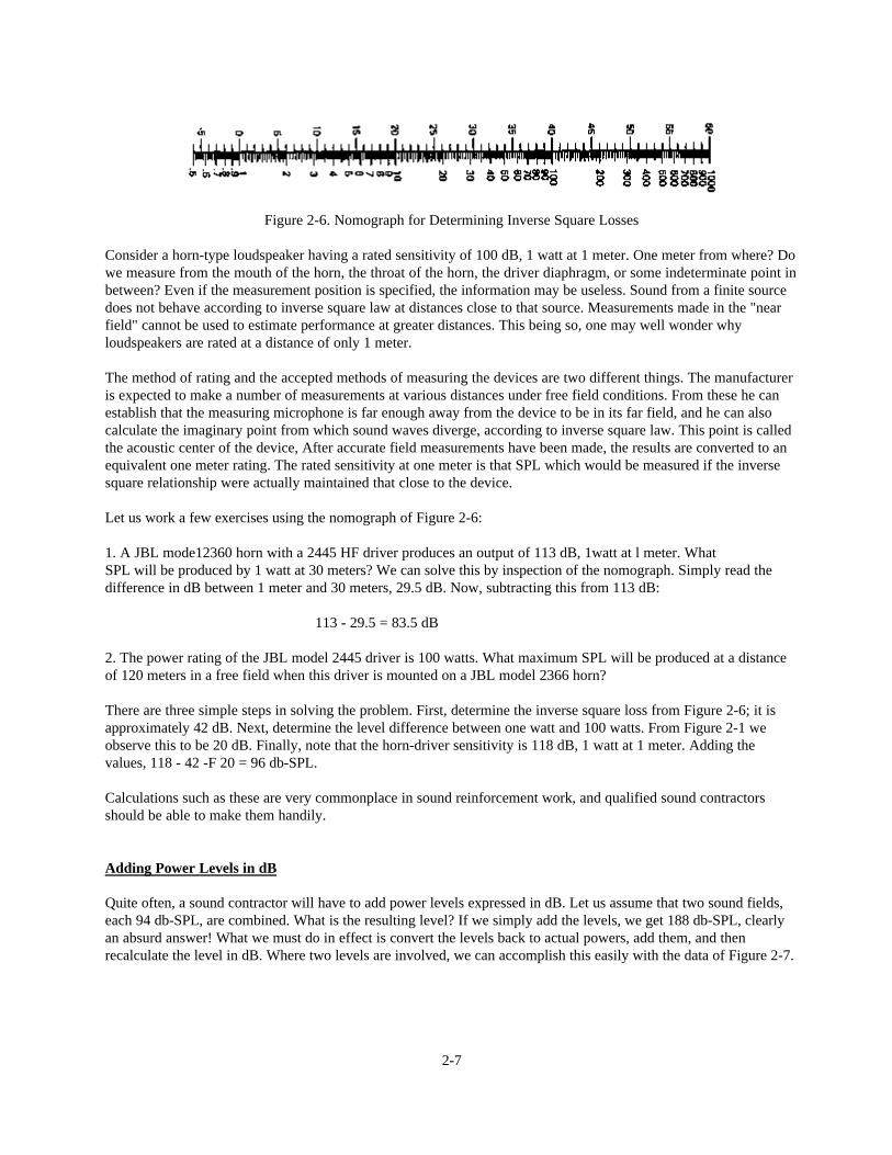
Figure 2-6. Nomograph for Determining Inverse Square Losses

Consider a horn-type loudspeaker having a rated sensitivity of 100 dB, 1 watt at 1 meter. One meter from where? Dowe measure from the mouth of the horn, the throat of the horn, the driver diaphragm, or some indeterminate point inbetween? Even if the measurement position is specified, the information may be useless. Sound from a finite sourcedoes not behave according to inverse square law at distances close to that source. Measurements made in the "nearfield" cannot be used to estimate performance at greater distances. This being so, one may well wonder whyloudspeakers are rated at a distance of only 1 meter.

The method of rating and the accepted methods of measuring the devices are two different things. The manufactureris expected to make a number of measurements at various distances under free field conditions. From these he canestablish that the measuring microphone is far enough away from the device to be in its far field, and he can alsocalculate the imaginary point from which sound waves diverge, according to inverse square law. This point is calledthe acoustic center of the device, After accurate field measurements have been made, the results are converted to anequivalent one meter rating. The rated sensitivity at one meter is that SPL which would be measured if the inversesquare relationship were actually maintained that close to the device.

Let us work a few exercises using the nomograph of Figure 2-6:

1. A JBL mode12360 horn with a 2445 HF driver produces an output of 113 dB, 1watt at l meter. WhatSPL will be produced by 1 watt at 30 meters? We can solve this by inspection of the nomograph. Simply read thedifference in dB between 1 meter and 30 meters, 29.5 dB. Now, subtracting this from 113 dB:

113 - 29.5 = 83.5 dB

2. The power rating of the JBL model 2445 driver is 100 watts. What maximum SPL will be produced at a distanceof 120 meters in a free field when this driver is mounted on a JBL model 2366 horn?

There are three simple steps in solving the problem. First, determine the inverse square loss from Figure 2-6; it isapproximately 42 dB. Next, determine the level difference between one watt and 100 watts. From Figure 2-1 weobserve this to be 20 dB. Finally, note that the horn-driver sensitivity is 118 dB, 1 watt at 1 meter. Adding thevalues, 118 - 42 -F 20 = 96 db-SPL.

Calculations such as these are very commonplace in sound reinforcement work, and qualified sound contractorsshould be able to make them handily.

Adding Power Levels in dB

Quite often, a sound contractor will have to add power levels expressed in dB. Let us assume that two sound fields,each 94 db-SPL, are combined. What is the resulting level? If we simply add the levels, we get 188 db-SPL, clearlyan absurd answer! What we must do in effect is convert the levels back to actual powers, add them, and thenrecalculate the level in dB. Where two levels are involved, we can accomplish this easily with the data of Figure 2-7.

2-7

D

N

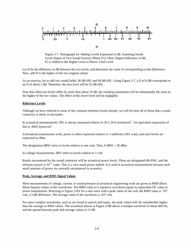
Figure 2-7. Nomograph for Adding Levels Expressed in dB. Summing SoundLevel Output of Two Sound Sources Where D is Their Output Difference in dB,N, is Added to the Higher Level to Derive Total Level

Let D be the difference in dB between the two levels, and.determine the value N corresponding to this difference.Now, add N to the higher of the two original values.

As an exercise, let us add two sound fields, 90 dB-SPL and 84 dB-SPL. Using Figure 2-7, a D of 6 dB corresponds toan N of about 1 dB. Therefore, the new level will be 91 dB-SPL.

Note that when two levels differ by more than about 10 dB, the resulting summation will be substantially the same asthe higher of the two values. The effect of the lower level will be negligible.

Reference Levels

Although we have referred to some of the common reference levels already, we will list here all of those that a soundcontractor is likely to encounter.

In acoustical measurements, SPL is always measured relative to 20 x 10-6 newtons/m2. An equivalent expression ofthis is .0002 dynes/cm2.

In broadcast transmission work, power is often expressed relative to 1 milliwatt (.001 watt), and such levels areexpressed as dBm.

The designation dBW refers to levels relative to one watt. Thus, 0 dBW = 30 dBm.

In voltage measurements, dBV refers to levels relative to 1 volt.

Rarely encountered by the sound contractor will be acoustical power levels. These are designated dB-PWL, and thereference power is 10-12 watts. This is a very small power indeed. It is used in acoustical measurements because suchsmall amounts of power are normally encountered in acoustics.

Peak, Average, and RMS Signal Values

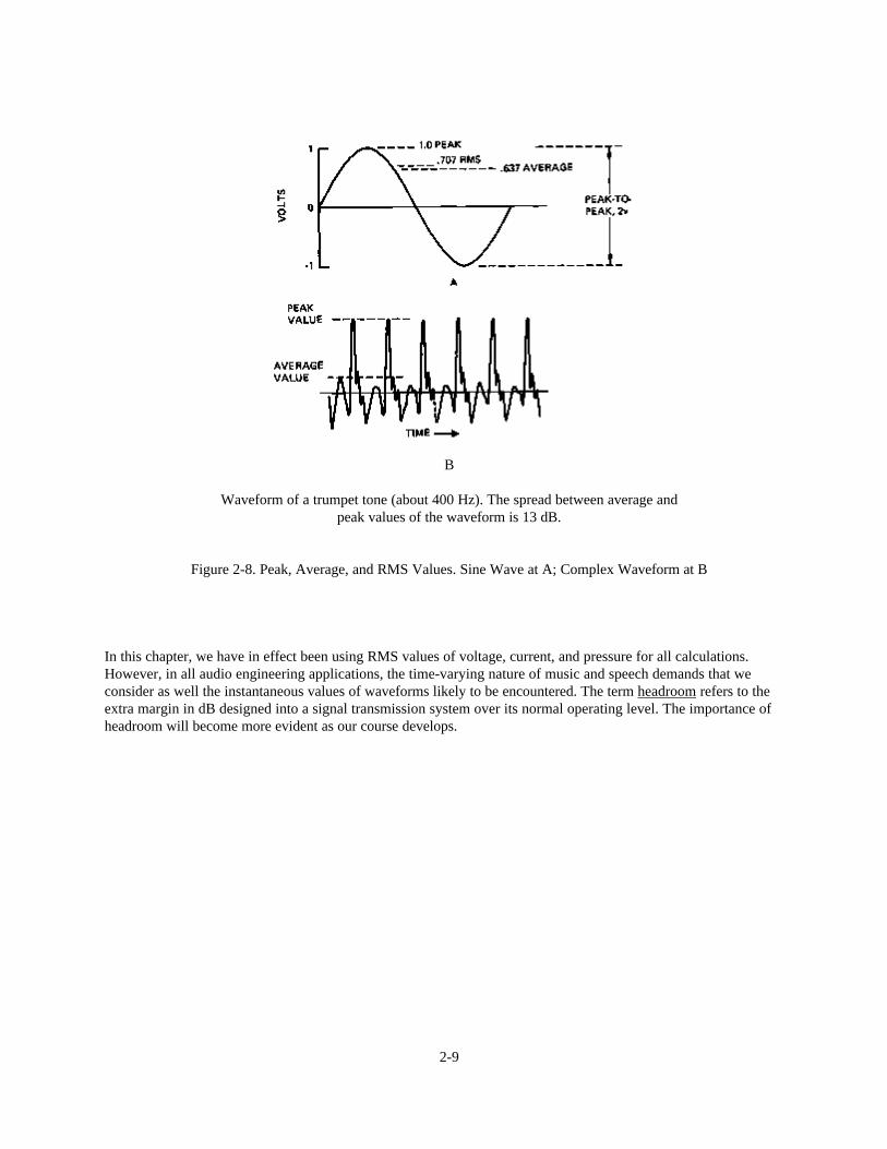
Most measurements of voltage, current, or sound pressure in acoustical engineering work are given as RMS (RootMean Square) values of the waveforms. The RMS value of a repetitive waveform equals its equivalent DC value inpower transmission. Referring to Figure 2-8A for a sine wave with a peak value of one volt, the RMS value is .707volt, a 3 dB difference. The average value of the waveform is .637 volt.

For more complex waveforms, such as are found in speech and music, the peak values will .be considerably higherthan the average or RMS values. The waveform shown at Figure 2-8B shows a trumpet waveform of about 400 Hz,and the spread between peak and average values is 13 dB.

2-8

B

Waveform of a trumpet tone (about 400 Hz). The spread between average andpeak values of the waveform is 13 dB.

Figure 2-8. Peak, Average, and RMS Values. Sine Wave at A; Complex Waveform at B

In this chapter, we have in effect been using RMS values of voltage, current, and pressure for all calculations.However, in all audio engineering applications, the time-varying nature of music and speech demands that weconsider as well the instantaneous values of waveforms likely to be encountered. The term headroom refers to theextra margin in dB designed into a signal transmission system over its normal operating level. The importance ofheadroom will become more evident as our course develops.

2-9

CHAPTER 3: DIRECTIVITY AND ANGULAR COVERAGE OF LOUDSPEAKERS

Introduction

Proper coverage of the audience area is one of the prime requirements of a sound reinforcement system.What is required of the sound contractor is not only a knowledge of the directional characteristics of variouscomponents but also how those components may interact in a multi-component array. Such terms as directivity index(DI), directivity factor (Q), and beamwidth all variously describe the directional properties of transducers with theirassociated horns and enclosures. Detailed polar data, when available, gives the most information of all. In general,no one has ever complained of having too much directivity information. In the past, most manufacturers havesupplied too little; however, things have changed for the better in recent years, largely through data standardizationactivities on the part of the Audio Engineering Society.

Some Fundamentals

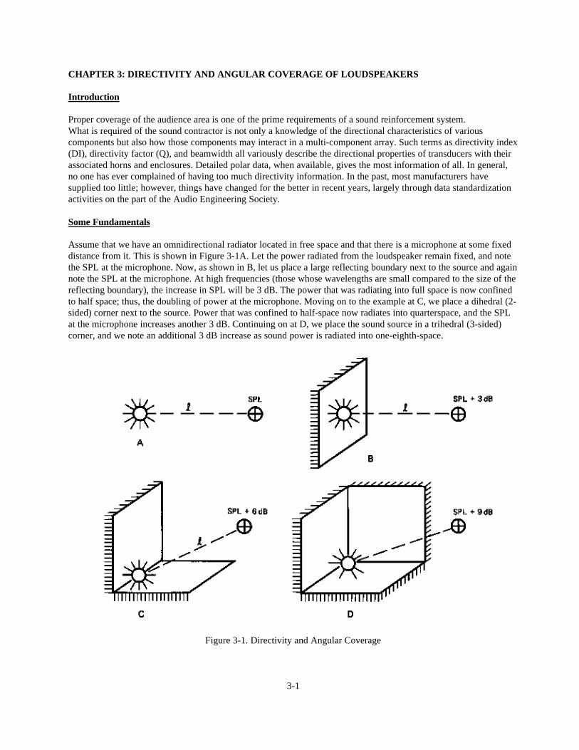
Assume that we have an omnidirectional radiator located in free space and that there is a microphone at some fixeddistance from it. This is shown in Figure 3-1A. Let the power radiated from the loudspeaker remain fixed, and notethe SPL at the microphone. Now, as shown in B, let us place a large reflecting boundary next to the source and againnote the SPL at the microphone. At high frequencies (those whose wavelengths are small compared to the size of thereflecting boundary), the increase in SPL will be 3 dB. The power that was radiating into full space is now confinedto half space; thus, the doubling of power at the microphone. Moving on to the example at C, we place a dihedral (2-sided) corner next to the source. Power that was confined to half-space now radiates into quarterspace, and the SPLat the microphone increases another 3 dB. Continuing on at D, we place the sound source in a trihedral (3-sided)corner, and we note an additional 3 dB increase as sound power is radiated into one-eighth-space.

Figure 3-1. Directivity and Angular Coverage

3-1

We could continue this exercise further, but our point has already been made. In going from A to D in successivesteps, we have increased the directivity index 3 dB at each step, and we have doubled the directivity factor at eachstep.

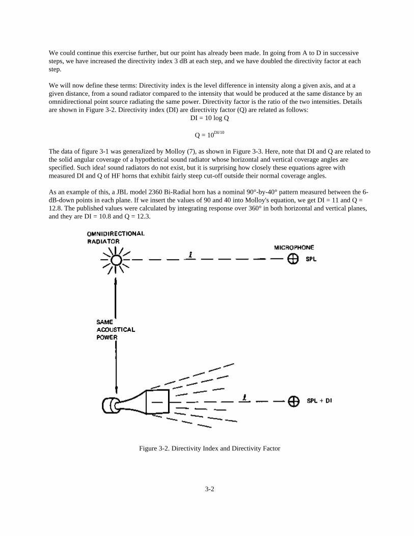
We will now define these terms: Directivity index is the level difference in intensity along a given axis, and at agiven distance, from a sound radiator compared to the intensity that would be produced at the same distance by anomnidirectional point source radiating the same power. Directivity factor is the ratio of the two intensities. Detailsare shown in Figure 3-2. Directivity index (DI) are directivity factor (Q) are related as follows:

DI = 10 log Q

Q = 10DI/10

The data of figure 3-1 was generaJized by Molloy (7), as shown in Figure 3-3. Here, note that DI and Q are related tothe solid angular coverage of a hypothetical sound radiator whose horizontal and vertical coverage angles arespecified. Such idea! sound radiators do not exist, but it is surprising how closely these equations agree withmeasured DI and Q of HF horns that exhibit fairly steep cut-off outside their normal coverage angles.

As an example of this, a JBL model 2360 Bi-Radial horn has a nominal 90°-by-40° pattern measured between the 6-dB-down points in each plane. If we insert the values of 90 and 40 into Molloy's equation, we get DI = 11 and Q =12.8. The published values were calculated by integrating response over 360° in both horizontal and vertical planes,and they are DI = 10.8 and Q = 12.3.

Figure 3-2. Directivity Index and Directivity Factor

3-2

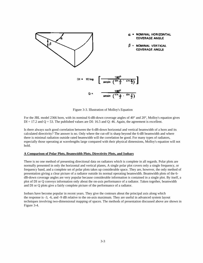
Figure 3-3. Illustration of Molloy's Equation

For the JBL model 2366 horn, with its nominal 6-dB-down coverage angles of 40° and 20°, Molloy's equation givesDI = 17.2 and Q = 53. The published values are DI: 16.5 and Q: 46. Again, the agreement is excellent.

Is there always such good correlation between the 6-dB-down horizontal and vertical beamwidth of a horn and itscalculated directivity? The answer is no. Only where the cut-off is sharp beyond the 6-dB beamwidth and wherethere is minimal radiation outside rated beamwidth will the correlation be good. For many types of radiators,especially those operating at wavelengths large compared with their physical dimensions, Molloy's equation will nothold.

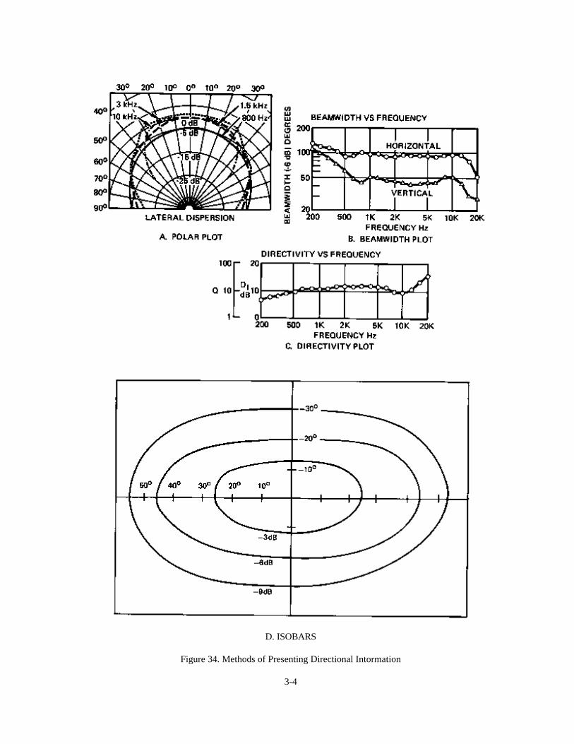
A Comparison of Polar Plots, Beamwidth Plots, Directivity Plots, and Isobars

There is no one method of presenting directional data on radiators which is complete in all regards. Polar plots arenormally presented in only the horizontal and vertical planes, A single polar plot covers only a single frequency, orfrequency band, and a complete set of polar plots takes up considerable space. They are, however, the only method ofpresentation giving a clear picture of a radiator outside its normal operating beamwidth. Beamwidth plots of the 6-dB-down coverage angles are very popular because considerable information is contained in a single plot. By itself, aplot of DI or Q conveys information only about the on-axis performance of a radiator. Taken together, beamwidthand DI or Q plots give a fairly complete picture of the performance of a radiator.

Isobars have become popular in recent years. They give the contours about the principal axis along whichthe response is -3, -6, and -9 dB relative to the on-axis maximum. They are useful in advanced system layouttechniques involving two-dimensional mapping of spaces. The methods of presentation discussed above are shown inFigure 3-4.

3-3

D. ISOBARS

Figure 34. Methods of Presenting Directional Intormation

3-4

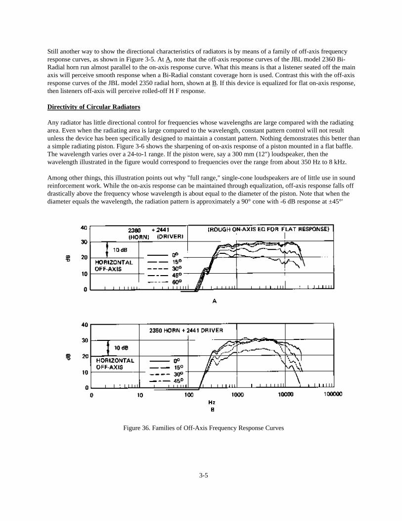
Still another way to show the directional characteristics of radiators is by means of a family of off-axis frequencyresponse curves, as shown in Figure 3-5. At A, note that the off-axis response curves of the JBL model 2360 Bi-Radial horn run almost parallel to the on-axis response curve. What this means is that a listener seated off the mainaxis will perceive smooth response when a Bi-Radial constant coverage horn is used. Contrast this with the off-axisresponse curves of the JBL model 2350 radial horn, shown at B. If this device is equalized for flat on-axis response,then listeners off-axis will perceive rolled-off H F response.

Directivity of Circular Radiators

Any radiator has little directional control for frequencies whose wavelengths are large compared with the radiatingarea. Even when the radiating area is large compared to the wavelength, constant pattern control will not resultunless the device has been specifically designed to maintain a constant pattern. Nothing demonstrates this better thana simple radiating piston. Figure 3-6 shows the sharpening of on-axis response of a piston mounted in a flat baffle.The wavelength varies over a 24-to-1 range. If the piston were, say a 300 mm (12") loudspeaker, then thewavelength illustrated in the figure would correspond to frequencies over the range from about 350 Hz to 8 kHz.

Among other things, this illustration points out why "full range," single-cone loudspeakers are of little use in soundreinforcement work. While the on-axis response can be maintained through equalization, off-axis response falls offdrastically above the frequency whose wavelength is about equal to the diameter of the piston. Note that when thediameter equals the wavelength, the radiation pattern is approximately a 90° cone with -6 dB response at ±45°'

Figure 36. Families of Off-Axis Frequency Response Curves

3-5

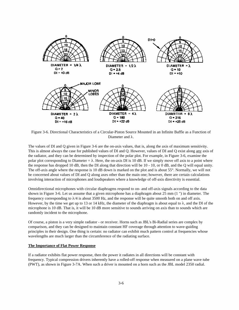
Figure 3-6. Directional Characteristics of a Circular-Piston Source Mounted in an Infinite Baffle as a Function ofDiameter and λ.

The values of DI and Q given in Figure 3-6 are the on-axis values, that is, along the axis of maximum sensitivity.This is almost always the case for published values of DI and Q. However, values of DI and Q exist along any axis ofthe radiator, and they can be determined by inspection of the polar plot. For example, in Figure 3-6, examine thepolar plot corresponding to Diameter = λ. Here, the on-axis DI is 10 dB. If we simply move off axis to a point wherethe response has dropped 10 dB, then the DI along that direction will be 10 - 10, or 0 dB, and the Q will equal unity.The off-axis angle where the response is 10 dB down is marked on the plot and is about 55°. Normally, we will notbe concerned about values of DI and Q along axes other than the main one; however, there are certain calculationsinvolving interaction of microphones and loudspeakers where a knowledge of off-axis directivity is essential.

Omnidirectional microphones with circular diaphragms respond to on- and off-axis signals according to the datashown in Figure 3-6. Let us assume that a given microphone has a diaphragm about 25 mm (1 ") in diameter. Thefrequency corresponding to λ/4 is about 3500 Hz, and the response will be quite smooth both on and off axis.However, by the time we get up to 13 or 14 kHz, the diameter of the diaphragm is about equal to λ, and the DI of themicrophone is 10 dB. That is, it will be 10 dB more sensitive to sounds arriving on axis than to sounds which arerandomly incident to the microphone.

Of course, a piston is a very simple radiator - or receiver. Horns such as JBL's Bi-Radial series are complex bycomparison, and they can be designed to maintain constant HF coverage through attention to wave-guidingprinciples in their design. One thing is certain: no radiator can exhibit much pattern control at frequencies whosewavelengths are much larger than the circumference of the radiating surface.

The Importance of Flat Power Response

If a radiator exhibits flat power response, then the power it radiates in all directions will be constant withfrequency. Typical compression drivers inherently have a rolled-off response when measured on a plane wave tube(PWT), as shown in Figure 3-7A. When such a driver is mounted on a horn such as the JBL model 2350 radial.

3-6

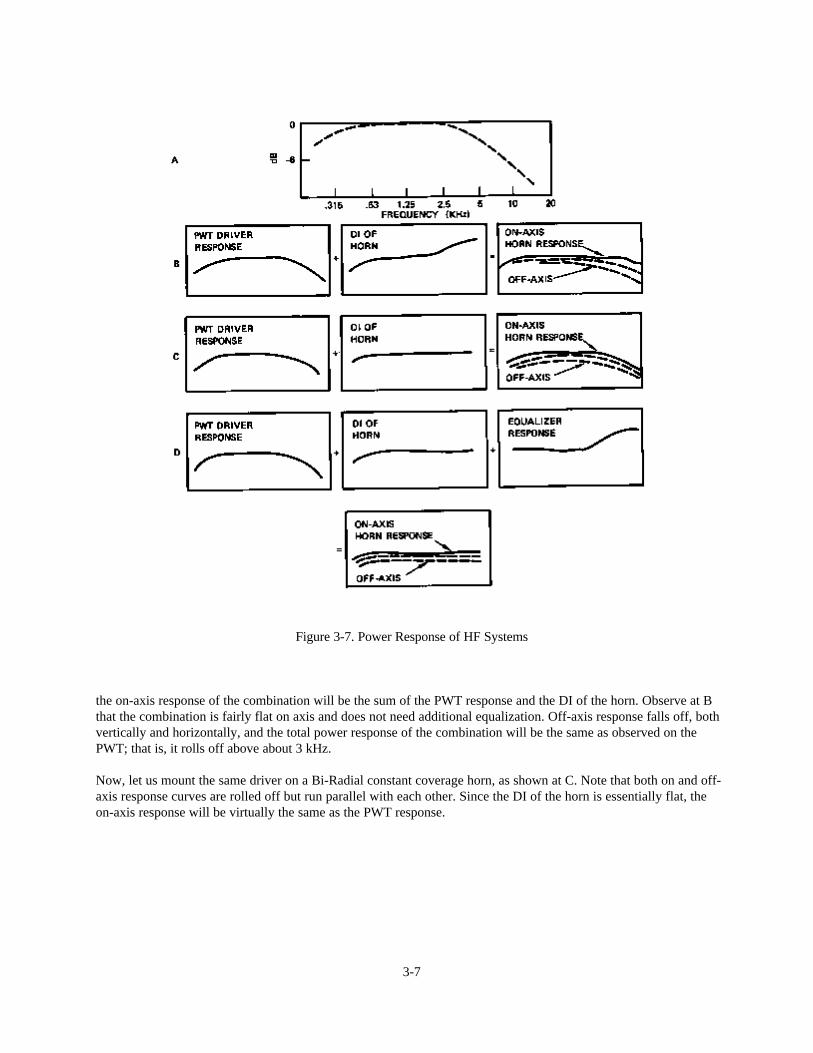
Figure 3-7. Power Response of HF Systems

the on-axis response of the combination will be the sum of the PWT response and the DI of the horn. Observe at Bthat the combination is fairly flat on axis and does not need additional equalization. Off-axis response falls off, bothvertically and horizontally, and the total power response of the combination will be the same as observed on thePWT; that is, it rolls off above about 3 kHz.

Now, let us mount the same driver on a Bi-Radial constant coverage horn, as shown at C. Note that both on and off-axis response curves are rolled off but run parallel with each other. Since the DI of the horn is essentially flat, theon-axis response will be virtually the same as the PWT response.

3-7

At D, we have inserted a HF boost to compensate for the driver's rolled off power response, and the result is flatresponse both on and off axis. Listeners anywhere in the area covered by the horn will appreciate the smooth andextended response of the system.

Flat power response makes sense only with components exhibiting constant angular coverage. If we had equalizedthe 2350 horn for flat power response, then the on-axis response would have been too bright and edgy sounding.

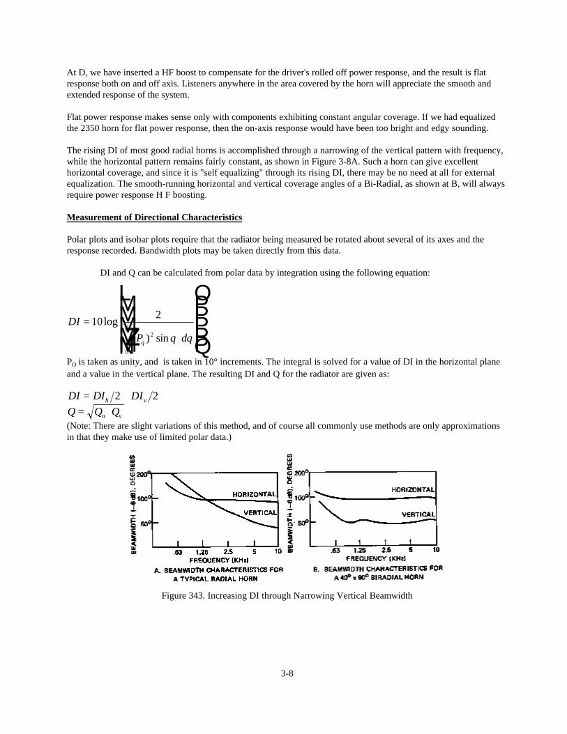
The rising DI of most good radial horns is accomplished through a narrowing of the vertical pattern with frequency,while the horizontal pattern remains fairly constant, as shown in Figure 3-8A. Such a horn can give excellenthorizontal coverage, and since it is "self equalizing" through its rising DI, there may be no need at all for externalequalization. The smooth-running horizontal and vertical coverage angles of a Bi-Radial, as shown at B, will alwaysrequire power response H F boosting.

Measurement of Directional Characteristics

Polar plots and isobar plots require that the radiator being measured be rotated about several of its axes and theresponse recorded. Bandwidth plots may be taken directly from this data.

DI and Q can be calculated from polar data by integration using the following equation:

DIP d

=⋅

L

N

MMMMM

O

Q

PPPPPz10 2

2

0

log( ) sinθ

π

θ θ

PO is taken as unity, and is taken in 10° increments. The integral is solved for a value of DI in the horizontal planeand a value in the vertical plane. The resulting DI and Q for the radiator are given as:

DI DI DIh v= +2 2Q Q Qn v= ⋅(Note: There are slight variations of this method, and of course all commonly use methods are only approximationsin that they make use of limited polar data.)

Figure 343. Increasing DI through Narrowing Vertical Beamwidth

3-8

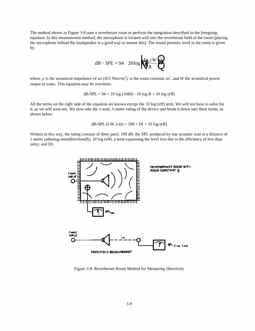
The method shown in Figure 3-9 uses a reverberant room to perform the integration described in the foregoingequation. In this measurement method, the microphone is located well into the reverberant field of the room (placingthe microphone behind the loudspeaker is a good way to ensure this). The sound pressure level in the room is givenby:

dB SPLcW

Ro− = + L

NMOQP94 20

41

2

logρ

where oc is the acoustical impedance of air (415 Nsec/m3), is the room constant, m2, and W the acoustical poweroutput in watts. This equation may be rewritten:

dB-SPL = 94 + 10 log (1660) - 10 log R + 10 log (eff)

All the terms on the right side of the equation are known except the 10 log (eff) term. We will not have to solve forit, as we will soon see. We now take the 1-watt, 1-meter rating of the device and break it down into three terms, asshown below:

dB-SPL (l-W, l-m) = 109 + DI + 10 log (eff)

Written in this way, the rating consists of three parts: 109 dB, the SPL produced by one acoustic watt at a distance of1 meter radiating omnidirectionally; 10 log (eff), a term expressing the level loss due to the efficiency of less thanunity; and DI.

Figure 3-9: Reverberant Room Method for Measuring Directivity

3-9

We now combine the two equations, eliminating the 10 log (eff) term:

DI = SPL(1-W, l-m) + 109 + 94 + 10 log (1660) - 10 log R - SPLREV - 10 log R

DI = SPL(1-W, l-m) + 17 - SPLREV - 10 log R

As an example using this method of measurement, we will consider a JBL 2360/2445 combination. The 1-watt, 1-meter rating is 113 dB-SPL, and the combination has been observed to produce a reverberant level of 108 dB-SPL ina live room with R = 18.6 m2. Using this equation:

DI = 113+ 17 - 108 - 10 log (18.6)

DI = 113+ 17 - 108 - 12.7 = 9.3dB

The value compares favorably with the published 10.8 dB. (Note: In explaining the foregoing method ofusing a live room for determining directivity, we have introduced the concepts of reverberation and room constantwithout defining them. These topics will be covered in detail in Chapter 5. It would be wise for the reader to go overthese examples again after Chapter 5 has been studied.)

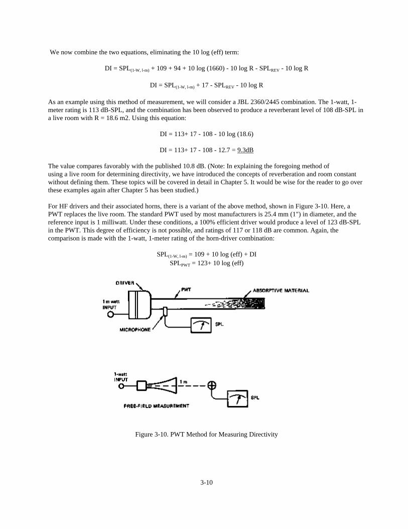
For HF drivers and their associated horns, there is a variant of the above method, shown in Figure 3-10. Here, aPWT replaces the live room. The standard PWT used by most manufacturers is 25.4 mm (1") in diameter, and thereference input is 1 milliwatt. Under these conditions, a 100% efficient driver would produce a level of 123 dB-SPLin the PWT. This degree of efficiency is not possible, and ratings of 117 or 118 dB are common. Again, thecomparison is made with the 1-watt, 1-meter rating of the horn-driver combination:

SPL(1-W, l-m) = 109 + 10 log (eff) + DISPLPWT = 123+ 10 log (eff)

Figure 3-10. PWT Method for Measuring Directivity

3-10

Eliminating the 10 log (eff) term:

DI = SPL(1-W, l-m) +14 - SPLPWT

As an example, the JBL 2445 HF driver is rated at 118 dB-SPL on a 25.4 mm PWT with a 1 mW input. The l-W, 1-m rating on the JBL 2365 horn is 115 dB-SPL. Thus:

DI = 115+ 14-118 = 11 dB

This compares favorably with the published value of 12.9 (1.7) dB.

Using Directivity Information

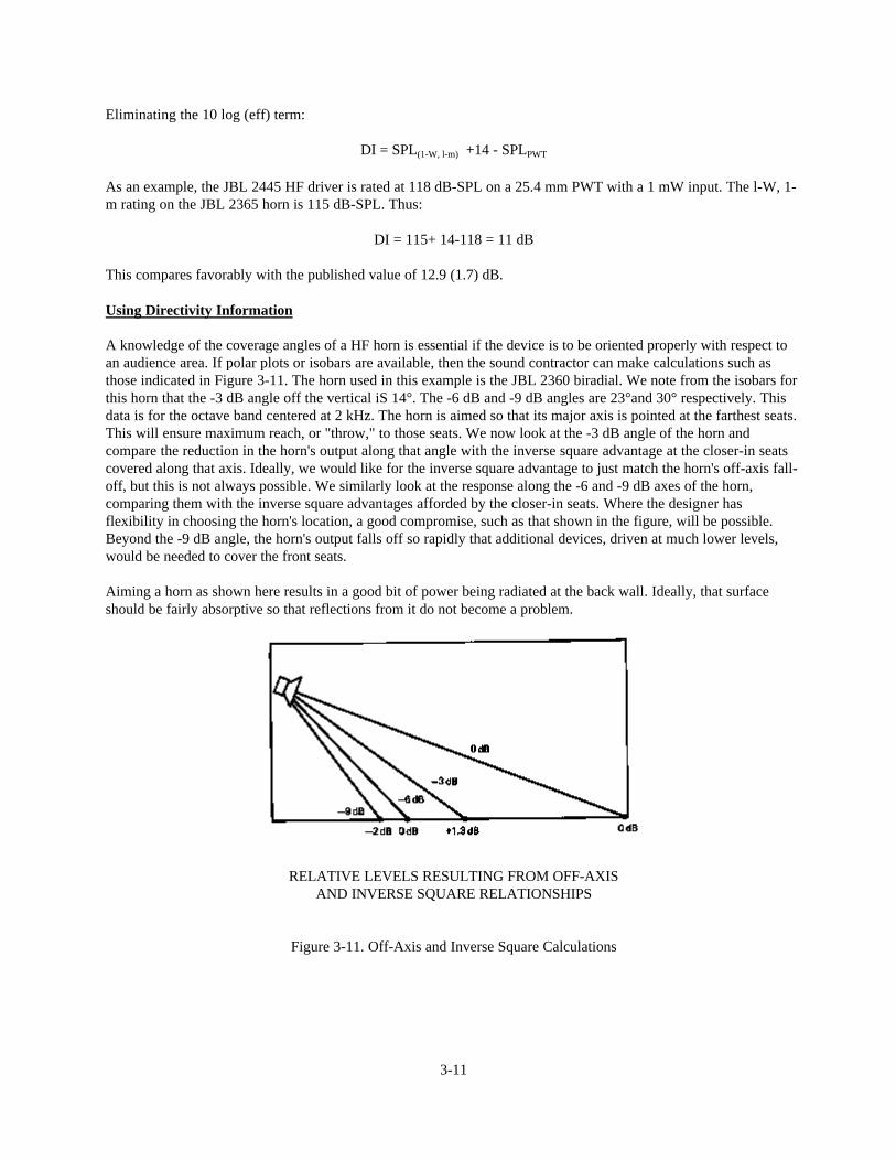
A knowledge of the coverage angles of a HF horn is essential if the device is to be oriented properly with respect toan audience area. If polar plots or isobars are available, then the sound contractor can make calculations such asthose indicated in Figure 3-11. The horn used in this example is the JBL 2360 biradial. We note from the isobars forthis horn that the -3 dB angle off the vertical iS 14°. The -6 dB and -9 dB angles are 23°and 30° respectively. Thisdata is for the octave band centered at 2 kHz. The horn is aimed so that its major axis is pointed at the farthest seats.This will ensure maximum reach, or "throw," to those seats. We now look at the -3 dB angle of the horn andcompare the reduction in the horn's output along that angle with the inverse square advantage at the closer-in seatscovered along that axis. Ideally, we would like for the inverse square advantage to just match the horn's off-axis fall-off, but this is not always possible. We similarly look at the response along the -6 and -9 dB axes of the horn,comparing them with the inverse square advantages afforded by the closer-in seats. Where the designer hasflexibility in choosing the horn's location, a good compromise, such as that shown in the figure, will be possible.Beyond the -9 dB angle, the horn's output falls off so rapidly that additional devices, driven at much lower levels,would be needed to cover the front seats.

Aiming a horn as shown here results in a good bit of power being radiated at the back wall. Ideally, that surfaceshould be fairly absorptive so that reflections from it do not become a problem.

RELATIVE LEVELS RESULTING FROM OFF-AXISAND INVERSE SQUARE RELATIONSHIPS

Figure 3-11. Off-Axis and Inverse Square Calculations

3-11

Directional Characteristics of Combined Radiators

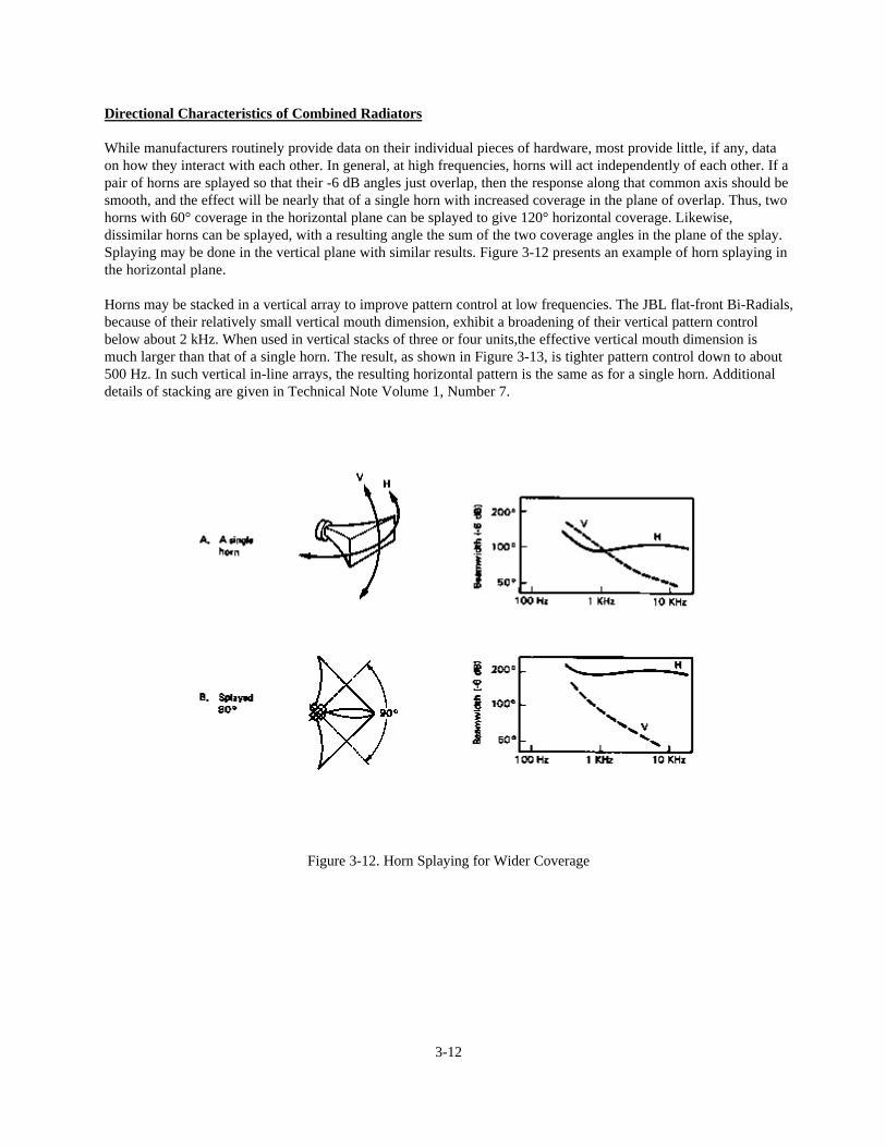
While manufacturers routinely provide data on their individual pieces of hardware, most provide little, if any, dataon how they interact with each other. In general, at high frequencies, horns will act independently of each other. If apair of horns are splayed so that their -6 dB angles just overlap, then the response along that common axis should besmooth, and the effect will be nearly that of a single horn with increased coverage in the plane of overlap. Thus, twohorns with 60° coverage in the horizontal plane can be splayed to give 120° horizontal coverage. Likewise,dissimilar horns can be splayed, with a resulting angle the sum of the two coverage angles in the plane of the splay.Splaying may be done in the vertical plane with similar results. Figure 3-12 presents an example of horn splaying inthe horizontal plane.

Horns may be stacked in a vertical array to improve pattern control at low frequencies. The JBL flat-front Bi-Radials,because of their relatively small vertical mouth dimension, exhibit a broadening of their vertical pattern controlbelow about 2 kHz. When used in vertical stacks of three or four units,the effective vertical mouth dimension ismuch larger than that of a single horn. The result, as shown in Figure 3-13, is tighter pattern control down to about500 Hz. In such vertical in-line arrays, the resulting horizontal pattern is the same as for a single horn. Additionaldetails of stacking are given in Technical Note Volume 1, Number 7.

Figure 3-12. Horn Splaying for Wider Coverage

3-12

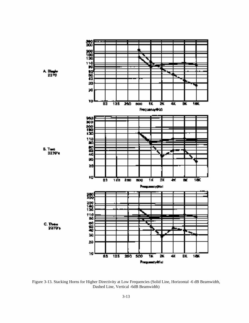
Figure 3-13. Stacking Horns for Higher Directivity at Low Frequencies (Solid Line, Horizontal -6 dB Beamwidth,Dashed Line, Vertical -6dB Beamwidth)

3-13

CHAPTER 4: AN OUTDOOR SOUND REINFORCEMENT SYSTEM

Introduction

Our study of sound reinforcement systems begins with an analysis of a simple outdoor system. The outdoorenvironment is relatively free of reflecting surfaces, and we will make the simplifying assumption that free fieldconditions exist. A basic reinforcement system is shown in Figure 4-1A. The essential acoustical elements are thetalker, microphone, loudspeaker, and listener. The electrical diagram of the system is shown at B. The dotted lineindicates the acoustical feedback path which exists around the electrical system.

When the system is turned on, the gain of the amplifier can be advanced up to some point at which the system will“ring,” or go into feedback. At the onset of feedback, the gain around the electro-acoustical path is unity and inphase. This condition is shown at C, where. the input at the microphone of a single pulse will give rise to a train ofpulses at the microphone produced by the loudspeaker. It can be seen that the process is self-sustaining, and acontinuing oscillation will exist.

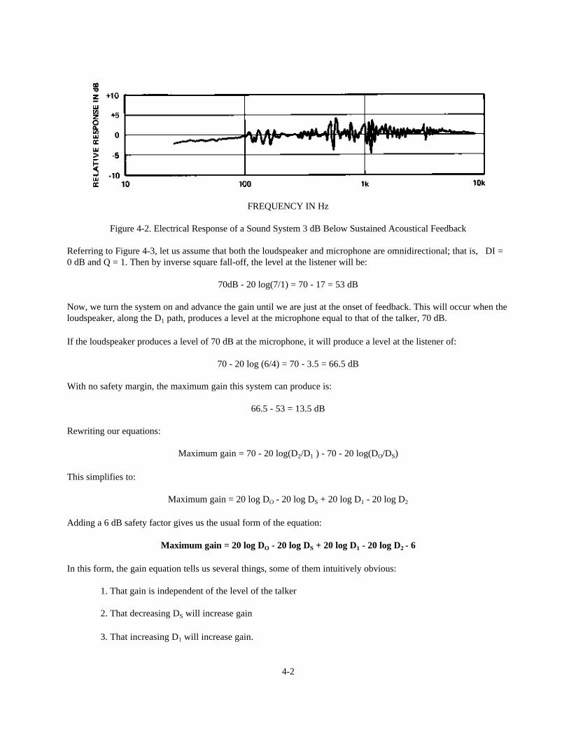
Even at levels somewhat below feedback, the response of the system will be irregular, due to the fact that the systemis “trying” to go into feedback, but does not have enough loop gain to sustain it. This is shown in Figure 4-2. As arule, a workable system should have a gain margin of 6 to 10 dB before feedback if it is to sound natural on all typesof program input.

The Concept of Acoustical Gain

Boner (4) quantified the concept of acoustical gain, and we will shortly present its simple but elegant derivation.Acoustical gain is defined as the increase in level that a given listener in the audience perceives with the systemturned on, as compared to the level he hears from the talker when the system is off.

Figure 4-1. A Simple Outdoor Reinforcement System

4-1

FREQUENCY IN Hz

Figure 4-2. Electrical Response of a Sound System 3 dB Below Sustained Acoustical Feedback

Referring to Figure 4-3, let us assume that both the loudspeaker and microphone are omnidirectional; that is, DI =0 dB and Q = 1. Then by inverse square fall-off, the level at the listener will be:

70dB - 20 log(7/1) = 70 - 17 = 53 dB

Now, we turn the system on and advance the gain until we are just at the onset of feedback. This will occur when theloudspeaker, along the D1 path, produces a level at the microphone equal to that of the talker, 70 dB.

If the loudspeaker produces a level of 70 dB at the microphone, it will produce a level at the listener of:

70 - 20 log (6/4) = 70 - 3.5 = 66.5 dB

With no safety margin, the maximum gain this system can produce is:

66.5 - 53 = 13.5 dB

Rewriting our equations:

Maximum gain = 70 - 20 log(D2/D1 ) - 70 - 20 log(DO/DS)

This simplifies to:

Maximum gain = 20 log DO - 20 log DS + 20 log D1 - 20 log D2

Adding a 6 dB safety factor gives us the usual form of the equation:

Maximum gain = 20 log DO - 20 log DS + 20 log D1 - 20 log D2 - 6

In this form, the gain equation tells us several things, some of them intuitively obvious:

1. That gain is independent of the level of the talker

2. That decreasing DS will increase gain

3. That increasing D1 will increase gain.

4-2

Figure 4-3. System Gain Calculations, Loudspeaker and Microphone Omnidirectional

The Influence of Directional Microphones and Loudspeakers on System Maximum Gain

Let us rework the example of Figure 4-3, this time making use of a directional loudspeaker whose polarcharacteristics are shown in Figure 4-4A. It is obvious from looking at Figure 4-4A that sound arriving at themicrophone along the D1 direction will be reduced 6 dB relative to the omnidirectional loudspeaker. This 6 dBresults directly in added gain potential for the system.

The same holds for directional microphones, as shown in Figure 4-5A. In Figure 4-5B, we show a system using anomnidirectional loudspeaker and a cardioid microphone with its -6 dB axis facing toward the loudspeaker. Thissystem is equivalent to the one shown in Figure 4-4B; both exhibit a 6 dB increase in maximum gain over the earliercase where both microphone and loudspeaker were omnidirectional.

Finally, we can use both directional loudspeakers and microphones to pick up additional gain. We simply calculatethe maximum gain using omnidirectional elements, and then add to it the off-axis advantage in dB for bothloudspeaker and microphone. As a practical matter, however, it is not wise to rely too heavily on directionalmicrophones and loudspeakers to increase system gain. Most designers are content to realize no more than 6 dBadded gain from the use of directional elements. The reason for this is that microphones and loudspeaker directionalpatterns are not constant with frequency. Most directional loudspeakers will, at low frequencies, appear to be nearlyomnidirectional. If more gain is called for, the most straightforward way to get it is to reduce DS or increase D1

How Much Gain is Needed?

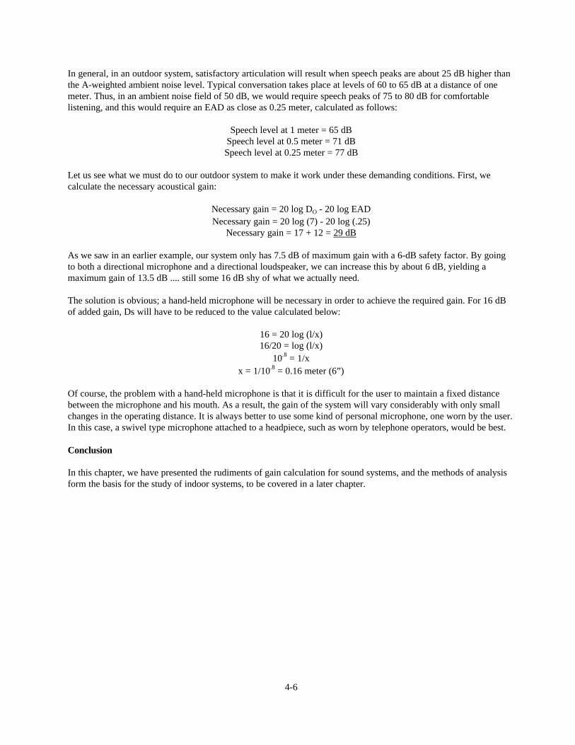
The parameters of a given sound reinforcement system may be such that we have more gain than we need. When thisis the case, we simply turn things down to a comfortable point, and everyone is happy. But things often do not workout so well. What is needed is some way of determining beforehand how much gain we will need so that we canavoid specifying a system which will not work. One way of doing this is by specifying the equivalent, or effective,acoustical distance (EAD), as shown in Figure 4-6. A sound reinforcement systems may be thought of as effectivelymoving the talker closer to the listener. In a quiet environment, we may not want to bring the talker any closer than,say, 3 meters from the listener. What this means, roughly, is that the loudness produced by the reinforcement systemshould approximate, for a listener at DO, the loudness level of an actual talker at a distance of 3 meters.

4-3

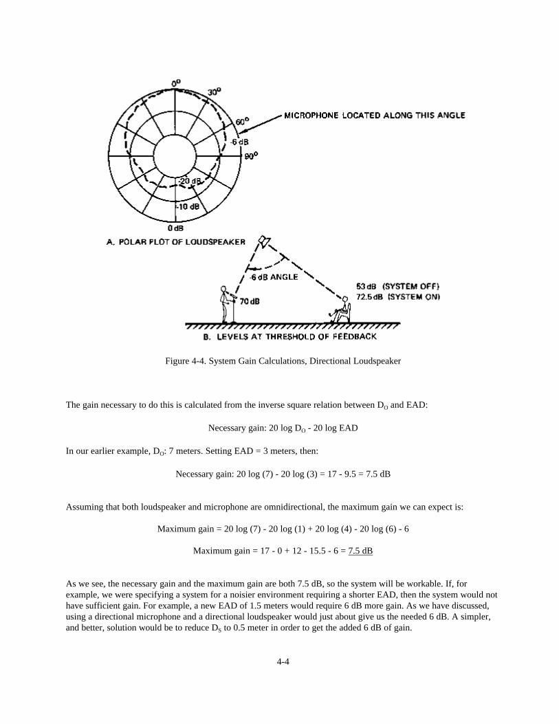
Figure 4-4. System Gain Calculations, Directional Loudspeaker

The gain necessary to do this is calculated from the inverse square relation between DO and EAD:

Necessary gain: 20 log DO - 20 log EAD

In our earlier example, DO: 7 meters. Setting EAD = 3 meters, then:

Necessary gain: 20 log (7) - 20 log (3) = 17 - 9.5 = 7.5 dB

Assuming that both loudspeaker and microphone are omnidirectional, the maximum gain we can expect is:

Maximum gain = 20 log (7) - 20 log (1) + 20 log (4) - 20 log (6) - 6

Maximum gain = 17 - 0 + 12 - 15.5 - 6 = 7.5 dB

As we see, the necessary gain and the maximum gain are both 7.5 dB, so the system will be workable. If, forexample, we were specifying a system for a noisier environment requiring a shorter EAD, then the system would nothave sufficient gain. For example, a new EAD of 1.5 meters would require 6 dB more gain. As we have discussed,using a directional microphone and a directional loudspeaker would just about give us the needed 6 dB. A simpler,and better, solution would be to reduce DS to 0.5 meter in order to get the added 6 dB of gain.

4-4

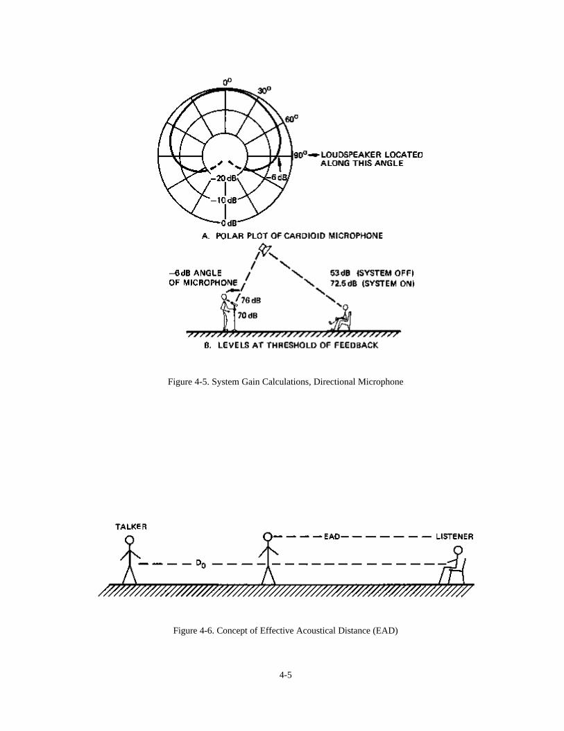
Figure 4-5. System Gain Calculations, Directional Microphone

Figure 4-6. Concept of Effective Acoustical Distance (EAD)

4-5

In general, in an outdoor system, satisfactory articulation will result when speech peaks are about 25 dB higher thanthe A-weighted ambient noise level. Typical conversation takes place at levels of 60 to 65 dB at a distance of onemeter. Thus, in an ambient noise field of 50 dB, we would require speech peaks of 75 to 80 dB for comfortablelistening, and this would require an EAD as close as 0.25 meter, calculated as follows:

Speech level at 1 meter = 65 dBSpeech level at 0.5 meter = 71 dBSpeech level at 0.25 meter = 77 dB

Let us see what we must do to our outdoor system to make it work under these demanding conditions. First, wecalculate the necessary acoustical gain:

Necessary gain = 20 log DO - 20 log EADNecessary gain = 20 log (7) - 20 log (.25)

Necessary gain = 17 + 12 = 29 dB

As we saw in an earlier example, our system only has 7.5 dB of maximum gain with a 6-dB safety factor. By goingto both a directional microphone and a directional loudspeaker, we can increase this by about 6 dB, yielding amaximum gain of 13.5 dB .... still some 16 dB shy of what we actually need.

The solution is obvious; a hand-held microphone will be necessary in order to achieve the required gain. For 16 dBof added gain, Ds will have to be reduced to the value calculated below:

16 = 20 log (l/x)16/20 = log (l/x)

10.8 = 1/xx = 1/10.8 = 0.16 meter (6”)

Of course, the problem with a hand-held microphone is that it is difficult for the user to maintain a fixed distancebetween the microphone and his mouth. As a result, the gain of the system will vary considerably with only smallchanges in the operating distance. It is always better to use some kind of personal microphone, one worn by the user.In this case, a swivel type microphone attached to a headpiece, such as worn by telephone operators, would be best.

Conclusion

In this chapter, we have presented the rudiments of gain calculation for sound systems, and the methods of analysisform the basis for the study of indoor systems, to be covered in a later chapter.

4-6

CHAPTER 5: FUNDAMENTALS OF ROOM ACOUSTICS

Introduction

Most sound reinforcement systems are located indoors, and the acoustical properties of the enclosed space have aprofound effect on the system's requirements and its performance. Our study begins with a discussion of soundabsorption and reflection, the growth and decay of sound fields in a room, reverberation, direct and reverberantsound fields, critical distance, and room constant.

If analyzed in detail, any enclosed space is quite complex acoustically. We will make many simplifications as weconstruct “statistical” models of rooms, our aim being to keep our calculations to a minimum, while maintainingaccuracy on the order of 10%, or ±1 dB.

Absorption and Reflection of Sound

Sound tends to “bend around” non-porous, small obstacles. However, large surfaces such as the boundaries of roomsare typically partially flexible and partially porous. As a result, when sound strikes such a surface, some of its energyis reflected, some is absorbed, and some is transmitted through the boundary and again propagated as sound waveson the other side. See Figure 5-1.

All three effects may vary with frequency and with the angle of incidence. In typical situations, they do not vary withsound intensity. Over the range of sound pressures commonly encountered in audio work, most constructionmaterials have the same characteristics of reflection, absorption and transmission whether struck by very weak orvery strong sound waves.

ALL THREE EFFECTS MAY VARY WITH FREQUENCY AND ANGLE OF INCIDENCE.THEY DO NOT VARY WITH INTENSITY IN TYPICAL SITUATIONS.

Figure 5-1. Sound Impinging Upon Large Boundary Surface

5-1

When dealing with the behavior of sound in an enclosed space, we must be able to estimate how much sound energywill be lost each time a sound wave strikes one of the boundary surfaces or one of the room objects.

Tables of absorption coefficients for common building materials as well as special “acoustical” materials can befound in any architectural acoustics textbook or in data sheets supplied by manufacturers of construction materials.

Unless otherwise specified in fine print, published sound absorption coefficients represent average absorption over allpossible angles of incidence. This is desirable from a practical standpoint since the random incidence coefficient fitsthe situation that exists in a typical enclosed space where sound waves rebound many times from each boundarysurface in almost all possible directions.

Absorption ratings normally are given for a number of different frequency bands. Typically, each band of frequenciesis one octave wide and standard center frequencies of 125, 250, 500, 1000 Hz, etc. are used. In sound system design,it usually is sufficient to know absorption characteristics of materials in three or four frequency ranges. In thishandbook, we make use of absorption ratings in the bands centered at 125 Hz, 1 kHz and 4 kHz.

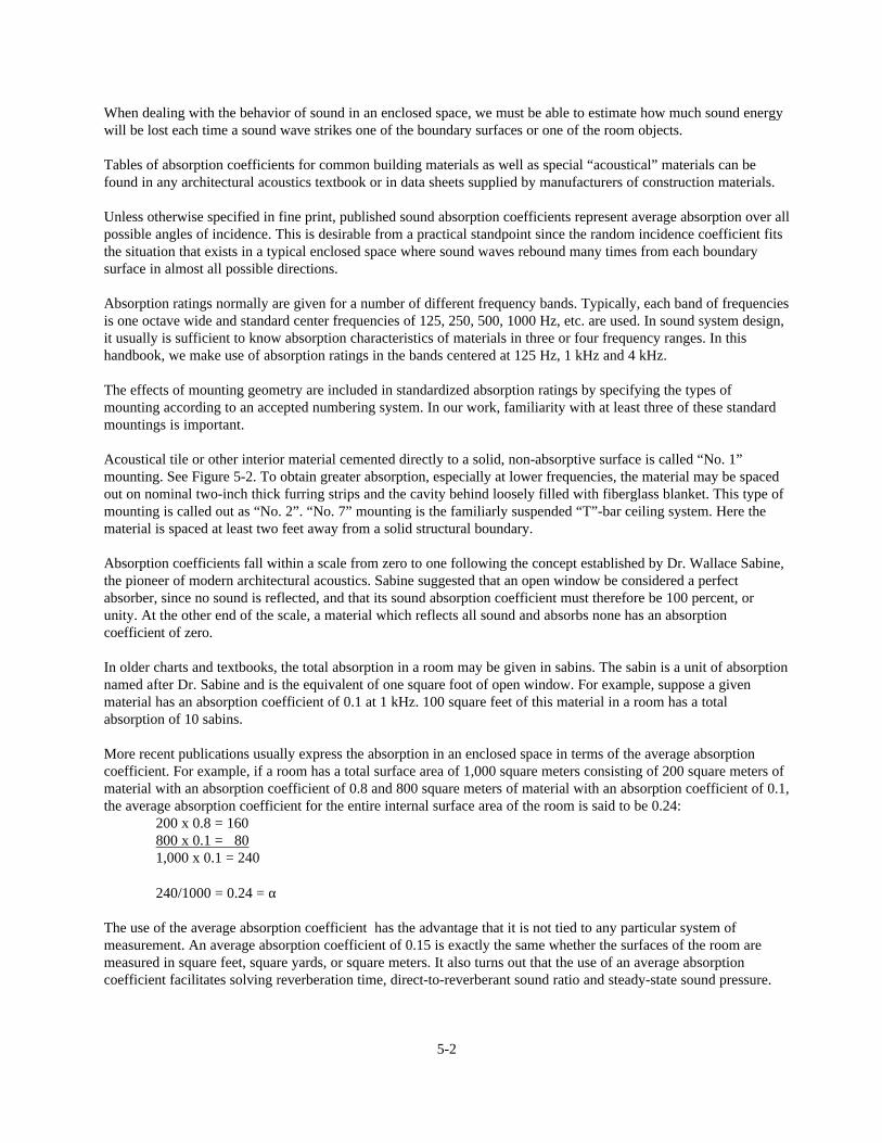
The effects of mounting geometry are included in standardized absorption ratings by specifying the types ofmounting according to an accepted numbering system. In our work, familiarity with at least three of these standardmountings is important.

Acoustical tile or other interior material cemented directly to a solid, non-absorptive surface is called “No. 1”mounting. See Figure 5-2. To obtain greater absorption, especially at lower frequencies, the material may be spacedout on nominal two-inch thick furring strips and the cavity behind loosely filled with fiberglass blanket. This type ofmounting is called out as “No. 2”. “No. 7” mounting is the familiarly suspended “T”-bar ceiling system. Here thematerial is spaced at least two feet away from a solid structural boundary.

Absorption coefficients fall within a scale from zero to one following the concept established by Dr. Wallace Sabine,the pioneer of modern architectural acoustics. Sabine suggested that an open window be considered a perfectabsorber, since no sound is reflected, and that its sound absorption coefficient must therefore be 100 percent, orunity. At the other end of the scale, a material which reflects all sound and absorbs none has an absorptioncoefficient of zero.

In older charts and textbooks, the total absorption in a room may be given in sabins. The sabin is a unit of absorptionnamed after Dr. Sabine and is the equivalent of one square foot of open window. For example, suppose a givenmaterial has an absorption coefficient of 0.1 at 1 kHz. 100 square feet of this material in a room has a totalabsorption of 10 sabins.

More recent publications usually express the absorption in an enclosed space in terms of the average absorptioncoefficient. For example, if a room has a total surface area of 1,000 square meters consisting of 200 square meters ofmaterial with an absorption coefficient of 0.8 and 800 square meters of material with an absorption coefficient of 0.1,the average absorption coefficient for the entire internal surface area of the room is said to be 0.24:

200 x 0.8 = 160800 x 0.1 = 801,000 x 0.1 = 240

240/1000 = 0.24 = α

The use of the average absorption coefficient has the advantage that it is not tied to any particular system ofmeasurement. An average absorption coefficient of 0.15 is exactly the same whether the surfaces of the room aremeasured in square feet, square yards, or square meters. It also turns out that the use of an average absorptioncoefficient facilitates solving reverberation time, direct-to-reverberant sound ratio and steady-state sound pressure.

5-2

Figure 5-2. ASTM Types of Mounting (Used in Conducting Sound Absorption Tests)

Although we commonly use published absorption coefficients without questioning their accuracy and perform simplearithmetic averaging to compute the average absorption coefficient of a room, the numbers themselves and theprocedures we use are only approximations. While this does not upset the reliability of our calculations to a largedegree, it is important to realize that the limit of confidence when working with published absorption coefficients isprobably somewhere in the neighborhood of ±10%.

How does the absorption coefficient of the material relate to the intensity of the reflected sound wave? An absorptioncoefficient of 0.2 at some specified frequency and angle of incidence means that 20% of the sound energy will beabsorbed and the remaining 80% reflected. The conversion to decibels is a simple 10 log function:

10 log10 0.8 = -0.97 dB

In the example given, the ratio of reflected to direct sound energy is about -1 dB. In other words, the reflected waveis 1 dB weaker than it would have been if the surface were 100% reflective. See the table in Figure 5-3.

Thinking in terms of decibels can be of real help in a practical situation. Suppose we want to improve the acousticsof a small auditorium which has a pronounced “slap” off the rear wall. To reduce the intensity of the slap by only 3dB, the wall must be surfaced with some material having an absorption coefficient of 0.5! To make the slap half asloud (a reduction of 10 dB) requires acoustical treatment of the rear wall to increase its absorption coefficient to 0.9.The difficulty is heightened by the fact that most materials absorb substantially less sound energy from a wavestriking head-on than their random incidence coefficients would indicate.

Most “acoustic” materials are porous. They belong to the class which acousticians elegantly label “fuzz”. Sound isabsorbed by offering resistance to the flow of air through the material and thereby changing some of the energy toheat.

5-3

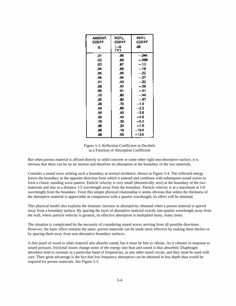
Figure 5-3. Reflection Coefficient in Decibelsas a Function of Absorption Coefficient

But when porous material is affixed directly to solid concrete or some other rigid non-absorptive surface, it isobvious that there can be no air motion and therefore no absorption at the boundary of the two materials.

Consider a sound wave striking such a boundary at normal incidence, shown in Figure 5-4. The reflected energyleaves the boundary in the opposite direction from which it entered and combines with subsequent sound waves toform a classic standing wave pattern. Particle velocity is very small (theoretically zero) at the boundary of the twomaterials and also at a distance 1/2 wavelength away from the boundary. Particle velocity is at a maximum at 1/4wavelength from the boundary. From this simple physical relationship it seems obvious that unless the thickness ofthe absorptive material is appreciable in comparison with a quarter wavelength, its effect will be minimal.

This physical model also explains the dramatic increase in absorptivity obtained when a porous material is spacedaway from a boundary surface. By spacing the layer of absorptive material exactly one-quarter wavelength away fromthe wall, where particle velocity is greatest, its effective absorption is multiplied many, many times.

The situation is complicated by the necessity of considering sound waves arriving from all possible directions.However, the basic effect remains the same: porous materials can be made more effective by making them thicker orby spacing them away from non-absorptive boundary surfaces.

A thin panel of wood or other material also absorbs sound, but it must be free to vibrate. As it vibrates in response tosound pressure, frictional losses change some of the energy into heat and sound is thus absorbed. Diaphragmabsorbers tend to resonate in a particular band of frequencies, as any other tuned circuit, and they must be used withcare. Their great advantage is the fact that low frequency absorption can be obtained in less depth than would berequired for porous materials. See Figure 5-5.

5-4

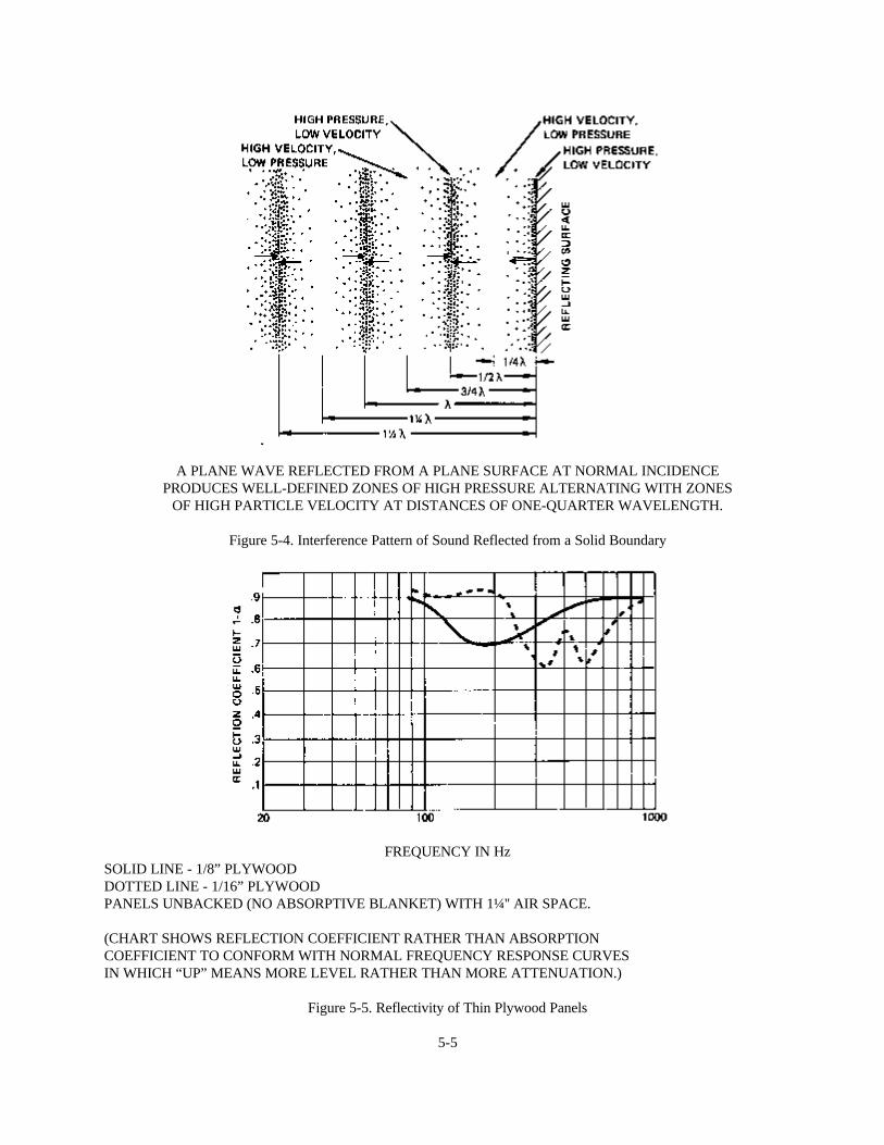
A PLANE WAVE REFLECTED FROM A PLANE SURFACE AT NORMAL INCIDENCEPRODUCES WELL-DEFINED ZONES OF HIGH PRESSURE ALTERNATING WITH ZONES

OF HIGH PARTICLE VELOCITY AT DISTANCES OF ONE-QUARTER WAVELENGTH.

Figure 5-4. Interference Pattern of Sound Reflected from a Solid Boundary

FREQUENCY IN HzSOLID LINE - 1/8” PLYWOODDOTTED LINE - 1/16” PLYWOODPANELS UNBACKED (NO ABSORPTIVE BLANKET) WITH 1¼'' AIR SPACE.

(CHART SHOWS REFLECTION COEFFICIENT RATHER THAN ABSORPTIONCOEFFICIENT TO CONFORM WITH NORMAL FREQUENCY RESPONSE CURVESIN WHICH “UP” MEANS MORE LEVEL RATHER THAN MORE ATTENUATION.)

Figure 5-5. Reflectivity of Thin Plywood Panels

5-5

A second type of tuned absorber occasionally used in acoustical work is the Helmholtz resonator: a reflex enclosurewithout a loudspeaker. (A patented construction material making use of this type of absorption is called“Soundblox”. These masonry blocks containing sound absorptive cavities can be used in gymnasiums, swimmingpools, and other locations in which porous materials cannot be employed.)

The Growth and Decay of a Sound Field in a Room

At this point we should have sufficient understanding of the behavior of sound in free space and the effects of largeboundary surfaces to understand what happens when sound is confined in an enclosure. The equations used todescribe the behavior of sound systems in rooms all involve considerable “averaging out” of complicated phenomena.Our calculations, therefore, are made on the basis of what is typical or normal; they do not give precise answers forparticular cases. In most situations, we can estimate with a considerable degree of confidence, but if we merely plugnumbers into equations without understanding the underlying physical processes, we may find ourselves makinglaborious calculations on the basis of pure guesswork without realizing it.

Suppose we have an omnidirectional sound source located somewhere near the center of a room. The source isturned on and from that instant sound radiates outward in all directions at 344 meters per second until it strikes theboundaries of the room. When sound strikes a boundary surface, some of the energy is absorbed, some is transmittedthrough the boundary and the remainder is reflected back into the room where it travels on a different course untilanother reflection occurs. After a certain length of time, so many reflections have taken place that the sound field is arandom jumble of waves traveling in all directions throughout the enclosed space.

If the source remains on and continues to emit sound at a steady rate, the energy inside the room builds up until astate of equilibrium is reached in which the sound energy being pumped into the room from the source exactlybalances the sound energy dissipated through absorption and transmission. Statistically, all of the individual soundpackets of varying intensities and varying directions can be averaged out, and at all points in the room not too closeto the source or any of the boundary surfaces, we can say that a uniform diffuse sound field exists.

The geometrical approach to architectural acoustics thus makes use of a sort of “soup” analogy. As long as asufficient number of reflections have taken place and as long as we can disregard such anomalies as strong focusedreflections, prominent resonant frequencies, the direct field near the source and the strong possibility that all roomsurfaces do not have the same absorption characteristics, this statistical model may be used to describe the soundfield in an actual room. In practice, the approach works remarkably well. If one is careful to allow for some of thefactors mentioned, theory allows us to make simple calculations regarding the behavior of sound in rooms and arriveat results sufficiently accurate for most noise control and sound system calculations.

Going back to our model, consider what happens when the sound source is turned off. Energy is no longer pumpedinto the room. Therefore, as a certain amount of energy is lost with each reflection, the energy density of the soundfield gradually decreases until all of the sound has been absorbed at the boundary surfaces.

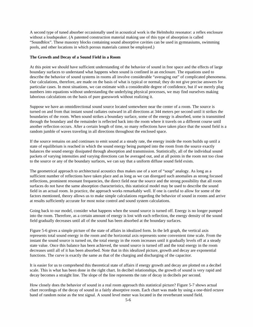
Figure 5-6 gives a simple picture of the state of affairs in idealized form. In the left graph, the vertical axisrepresents total sound energy in the room and the horizontal axis represents some convenient time scale. From theinstant the sound source is turned on, the total energy in the room increases until it gradually levels off at a steadystate value. Once this balance has been achieved, the sound source is turned off and the total energy in the roomdecreases until all of it has been absorbed. Note that in this idealized picture, growth and decay are exponentialfunctions. The curve is exactly the same as that of the charging and discharging of the capacitor.

It is easier for us to comprehend this theoretical state of affairs if energy growth and decay are plotted on a decibelscale. This is what has been done in the right chart. In decibel relationships, the growth of sound is very rapid anddecay becomes a straight line. The slope of the line represents the rate of decay in decibels per second.

How closely does the behavior of sound in a real room approach this statistical picture? Figure 5-7 shows actualchart recordings of the decay of sound in a fairly absorptive room. Each chart was made by using a one-third octaveband of random noise as the test signal. A sound level meter was located in the reverberant sound field.

5-6

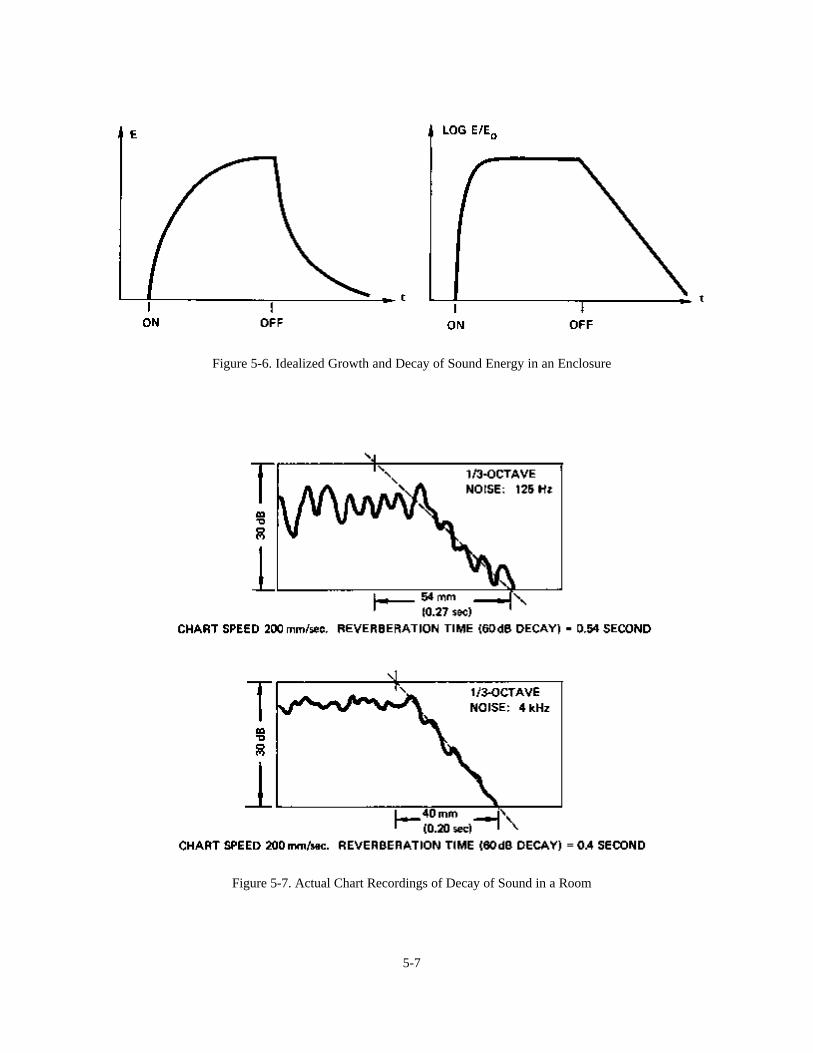
Figure 5-6. Idealized Growth and Decay of Sound Energy in an Enclosure

Figure 5-7. Actual Chart Recordings of Decay of Sound in a Room

5-7

(In practice several readings would be taken at a number of different locations in the room). The upper graphillustrates a measurement made in the band centered at 125 Hz. Note the great fluctuations in the steady state leveland similar fluctuations as the sound intensity decreases. The fluctuations are sufficiently great to make any “exact”determination of the decay rate impossible. Instead, a straight line which seems to represent the “best fit” is drawnand its slope measured. In this case, the slope of the line is such that sound pressure seems to be decaying at a rate of30 decibels per 0.27 seconds. This works out to a decay rate of 111 dB per second.

The lower chart shows a similar measurement taken with the one-third octave band centered at 4 kHz. Thefluctuations in level are not as pronounced and it is much easier to arrive at what seems to be the correct slope of thesound decay. In this instance sound pressure seems to be decreasing at a rate of 30 dB in 0.2 seconds, or a decay rateof 150 dB per second.

Reverberation and Reverberation Time

The term “decay rate” is relatively unfamiliar; usually we talk about “reverberation time”. Reverberation time wasoriginally described simply as the length of time required for a very loud sound to die away to inaudibility. It waslater defined in scientific terms as the length of time required for sound to decay 60 decibels. In both definitions it isassumed that decay rate is uniform and that the ambient noise level is low enough to be ignored.

In the real world, the decay rate in a particular band of frequencies may not be uniform and it may be very difficult tomeasure accurately over a 60 dB range. Most acousticians are satisfied to measure the first 30 dB decay after a testsignal is turned off and to use the slope of this portion of the curve to define the average decay rate and thereverberation time. In the example just given, estimates must be made over a useful range of only 20 dB or so.However, the height of the chart paper corresponds to a total range of 30 dB and this makes calculation ofreverberation time quite simple. At 125 Hz a sloping line drawn across the full width of the chart paper is equivalentto a 30 dB decay in 0.27 seconds. Reverberation time (60 dB decay) must, therefore, equal 0.54 seconds. Similarly,the same room has a reverberation time of only 0.4 seconds in the 4 kHz band.

In his original work in architectural acoustics, Wallace Sabine assumed the idealized exponential growth and decayof sound that was diagrammed in Figure 5-6. However, his equation based on this model was found to be inaccuratein rooms having substantial absorption. In other words, the Sabine equation works well in live rooms, but not inmoderately dead ones. In the 1920's and 1930's, a great deal of work was done in an effort to arrive at a model thatwould more accurately describe the growth and decay of sound in all types of rooms. On the basis of the materialpresented thus far, let us see if we can construct such a model.

We start by accepting the notion of a uniform diffuse steady state sound field. Even though the sound field in a realroom may fluctuate and though it may not be exactly the same at every point in the room, some sort of overallintensity average seems to be a reasonable simplifying assumption.

If we can average out variations in the sound field throughout the room, perhaps we can also find an averagedistance that sound can travel before bumping into one of the boundary surfaces. This notion of an average distancebetween bounces is more accurately known as the mean free path and is a common statistical notion in otherbranches of physics. For typical rooms, the mean free path turns out to be 4V/S, where V is enclosed volume and S isthe area of the boundary surfaces. Since sound waves will have bounced around all parts of the room striking all ofthe boundary surfaces in almost all possible angles before being completely absorbed, it seems reasonable that thereshould be some sort of average absorption coefficient α which would describe the total boundary surface area. Wewill use the simple arithmetic averaging technique to calculate this coefficient.

At this point we have postulated a highly simplified acoustical model which assumes that, on the average, the steadystate sound intensity in an actual room can be represented by a single number. We also have assumed that, on theaverage, sound waves in this room travel a distance equivalent to 4V/S between bounces. Finally, we have assumedthat, on the average, each time sound encounters a boundary surface it impinges upon a material having a randomincidence absorption coefficient denoted by a single number α.

5-8

Only one step remains to complete our model. Since sound travels at a known rate of speed, the mean freepath is equivalent to a certain mean free time between bounces.

Now imagine what must happen if we apply our model to the situation that exists in a room immediately after auniformly emitting sound source has been turned off. The sound waves continue to travel for a distance equal to themean free path. At this point they encounter a boundary surface having an absorption coefficient of α and a certainpercentage of the energy is lost. The remaining energy is reflected back into the room and again travels a distanceequal to the mean free path before encountering another boundary with absorption coefficient α. Each time sound isbounced off the boundary surface its energy is decreased by a proportion determined by the average absorptioncoefficient α.

If we know the proportion of energy lost with each bounce and the length of time between bounces, we cancalculate the average rate of decay and the reverberation time for a particular room.

Example: Consider a room 5m x 6m x 3m, as diagrammed in Figure 5-8. Let us calculate the decay rate andreverberation time for the octave band centered at 1 kHz.

The volume of the room is 90 cubic meters, and its total surface area is 126 square meters; therefore, the meanfree path 4V/S works out to be about 3 meters.

The next step is to list individually the areas and absorption coefficient of the various materials used on roomsurfaces, as is shown in the Figure.

The total surface area is 126 square meters; the total absorption (Sα.) adds up to 24.9 absorption units. Therefore,the average absorption coefficient (α) is 24.9 divided by 126, or 0.2.

Figure 5-8. Calculating Reverberation Time

5-9

If each reflection results in a decrease in energy of 0.2, the reflected wave must have an equivalent energy of 0.8. Aratio of 0.8 to 1 is equivalent to a loss of 0.97 decibel per reflection. For simplicity, let us call it 1 dB per reflection.

Since the mean free path is 2.9 meters, the mean free time must be about 0.008 seconds (2.9/334 = 0.008)

We now know that the rate of decay is equivalent to 1 dB per 0.008 seconds. The time for sound to decay 60 dBmust, therefore, be 60 x 0.008 = 0.48 seconds.

The Eyring equation in its standard form is shown in Figure 5-9. If this equation is used to calculate thereverberation of our hypothetical room, the answer comes out 0.482 seconds. If the Sabine formula is used tocalculate the reverberation time of this room, it provides an answer of 0.535 seconds or a discrepancy of a little morethan 10%.

Figure 5-9. Reverberation Time Equations

5-10

Rather than go through the calculations, it is much faster to use a simple chart. Charts calculated from the Eyringformula are given in Figures 5-10 and 5-11. Using the chart as a reference and again checking our hypotheticalexample, we find that a room having a mean free path just a little less than 3 meters and an average absorptioncoefficient of 0.2 must have a reverberation time of just a little less than 0.5 seconds.

Since reverberation time is directly proportional to the mean free path, it is desirable to calculate the latter asaccurately as possible. However, this is not the only area of uncertainty in these equations. There is argument amongacousticians as to whether published absorption coefficients, such as those of Figure 5-12, really correspond to therandom incidence absorption implicit in the Eyring equation. There also is argument over the method used to findthe “average” absorption coefficient for a room. In our example, we performed a simple arithmetic calculation to findthe average absorption coefficient. It has been pointed out that this is an unwarranted simplification; that the actualstate of affairs requires neither an arithmetic average nor a geometric mean, but some relation considerably morecomplicated than either.

Another source of uncertainty lies in determining the absorption coefficients of materials in situations other thanthose used to establish the rating. We know, for example, that the total absorption of a single large patch of materialis less than if the same amount of material is spread over a number of separated patches. At higher frequencies, airabsorption reduces reverberation time. Figure 5-13 can be used to estimate such deviations above 2 kHz.

A final source of uncertainty is inherent in the statistical nature of the model itself. We know from experience thatreverberation time in a large concert hall may be different in the seating area than if measured out near the center ofthe enclosed space.

Figure 5-10. Reverberation Time Chart, SI Units

5-11

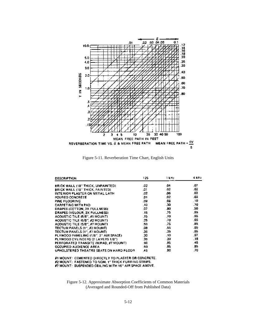
Figure 5-11. Reverberation Time Chart, English Units

Figure 5-12. Approximate Absorption Coefficients of Common Materials(Averaged and Rounded-Off from Published Data)

5-12

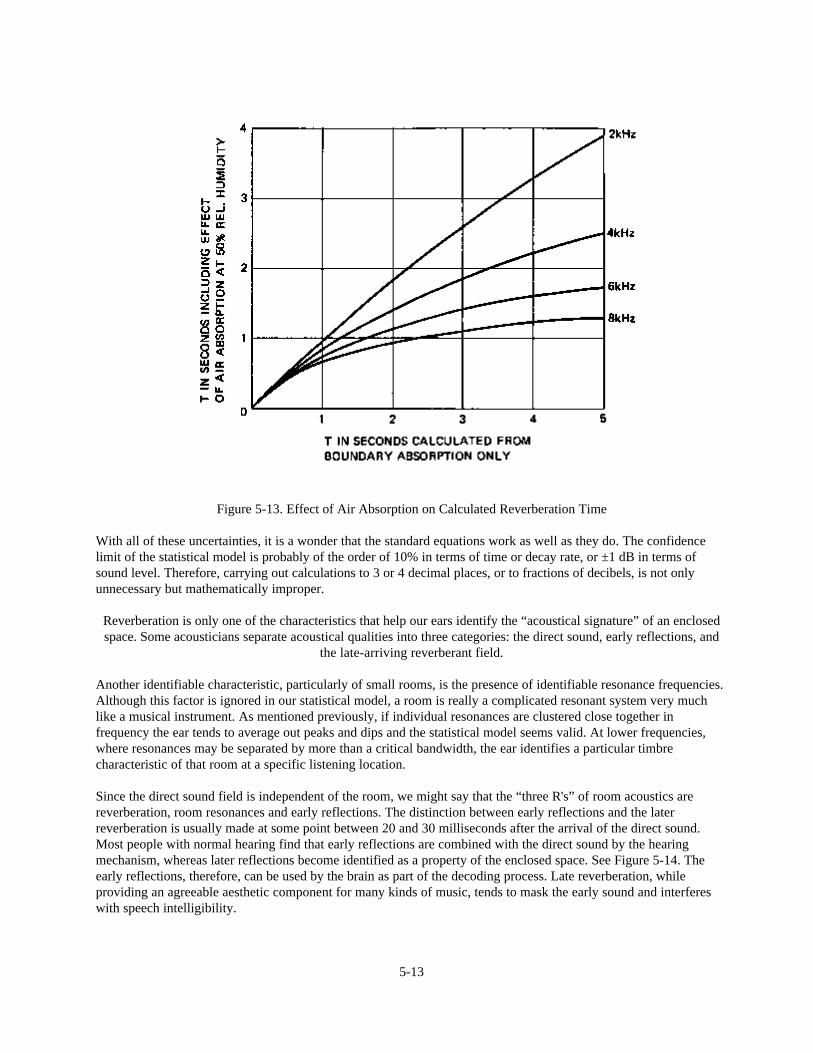
Figure 5-13. Effect of Air Absorption on Calculated Reverberation Time

With all of these uncertainties, it is a wonder that the standard equations work as well as they do. The confidencelimit of the statistical model is probably of the order of 10% in terms of time or decay rate, or ±1 dB in terms ofsound level. Therefore, carrying out calculations to 3 or 4 decimal places, or to fractions of decibels, is not onlyunnecessary but mathematically improper.

Reverberation is only one of the characteristics that help our ears identify the “acoustical signature” of an enclosedspace. Some acousticians separate acoustical qualities into three categories: the direct sound, early reflections, and

the late-arriving reverberant field.

Another identifiable characteristic, particularly of small rooms, is the presence of identifiable resonance frequencies.Although this factor is ignored in our statistical model, a room is really a complicated resonant system very muchlike a musical instrument. As mentioned previously, if individual resonances are clustered close together infrequency the ear tends to average out peaks and dips and the statistical model seems valid. At lower frequencies,where resonances may be separated by more than a critical bandwidth, the ear identifies a particular timbrecharacteristic of that room at a specific listening location.

Since the direct sound field is independent of the room, we might say that the “three R's” of room acoustics arereverberation, room resonances and early reflections. The distinction between early reflections and the laterreverberation is usually made at some point between 20 and 30 milliseconds after the arrival of the direct sound.Most people with normal hearing find that early reflections are combined with the direct sound by the hearingmechanism, whereas later reflections become identified as a property of the enclosed space. See Figure 5-14. Theearly reflections, therefore, can be used by the brain as part of the decoding process. Late reverberation, whileproviding an agreeable aesthetic component for many kinds of music, tends to mask the early sound and interfereswith speech intelligibility.

5-13

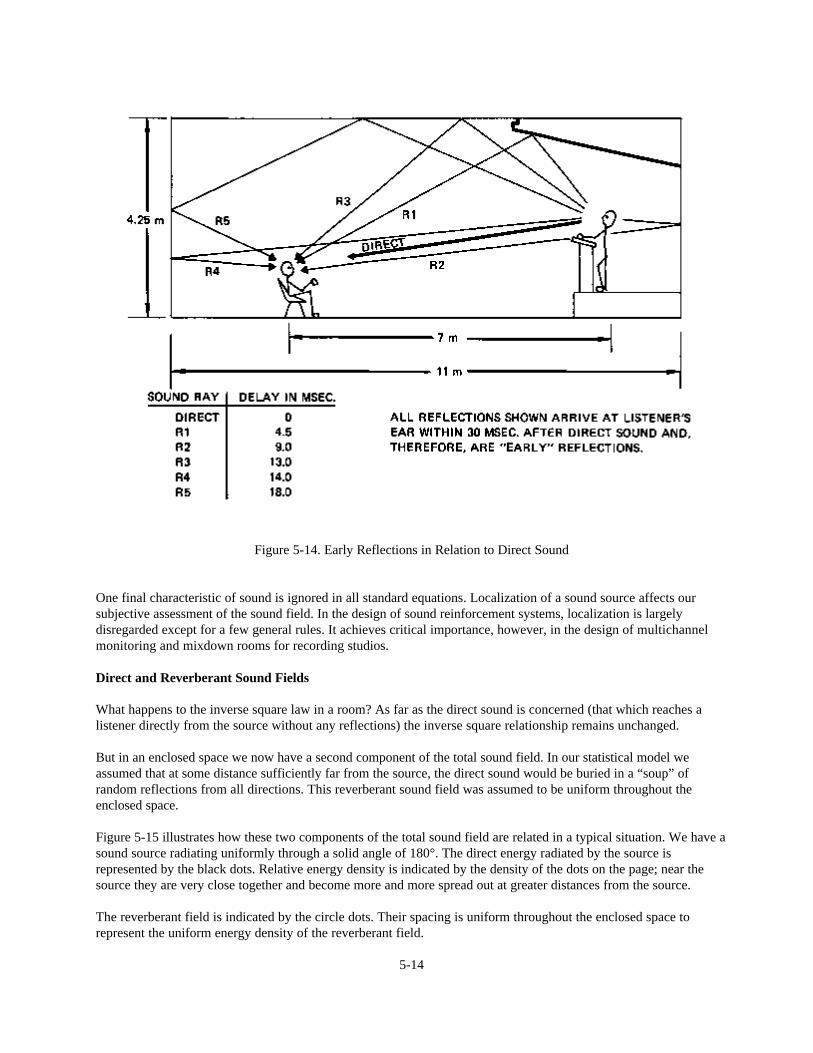
Figure 5-14. Early Reflections in Relation to Direct Sound

One final characteristic of sound is ignored in all standard equations. Localization of a sound source affects oursubjective assessment of the sound field. In the design of sound reinforcement systems, localization is largelydisregarded except for a few general rules. It achieves critical importance, however, in the design of multichannelmonitoring and mixdown rooms for recording studios.

Direct and Reverberant Sound Fields

What happens to the inverse square law in a room? As far as the direct sound is concerned (that which reaches alistener directly from the source without any reflections) the inverse square relationship remains unchanged.

But in an enclosed space we now have a second component of the total sound field. In our statistical model weassumed that at some distance sufficiently far from the source, the direct sound would be buried in a “soup” ofrandom reflections from all directions. This reverberant sound field was assumed to be uniform throughout theenclosed space.

Figure 5-15 illustrates how these two components of the total sound field are related in a typical situation. We have asound source radiating uniformly through a solid angle of 180°. The direct energy radiated by the source isrepresented by the black dots. Relative energy density is indicated by the density of the dots on the page; near thesource they are very close together and become more and more spread out at greater distances from the source.

The reverberant field is indicated by the circle dots. Their spacing is uniform throughout the enclosed space torepresent the uniform energy density of the reverberant field.

5-14

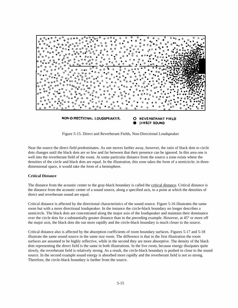
Figure 5-15. Direct and Reverberant Fields, Non-Directional Loudspeaker

Near the source the direct field predominates. As one moves farther away, however, the ratio of black dots to circledots changes until the black dots are so few and far between that their presence can be ignored. In this area one iswell into the reverberant field of the room. At some particular distance from the source a zone exists where thedensities of the circle and black dots are equal. In the illustration, this zone takes the form of a semicircle; in three-dimensional space, it would take the form of a hemisphere.

Critical Distance

The distance from the acoustic center to the gray-black boundary is called the critical distance. Critical distance isthe distance from the acoustic center of a sound source, along a specified axis, to a point at which the densities ofdirect and reverberant sound are equal.

Critical distance is affected by the directional characteristics of the sound source. Figure 5-16 illustrates the sameroom but with a more directional loudspeaker. In the instance the circle-black boundary no longer describes asemicircle. The black dots are concentrated along the major axis of the loudspeaker and maintain their dominanceover the circle dots for a substantially greater distance than in the preceding example. However, at 45° or more offthe major axis, the black dots die out more rapidly and the circle-black boundary is much closer to the source.

Critical distance also is affected by the absorption coefficients of room boundary surfaces. Figures 5-17 and 5-18illustrate the same sound source in the same size room. The difference is that in the first illustration the roomsurfaces are assumed to be highly reflective, while in the second they are more absorptive. The density of the blackdots representing the direct field is the same in both illustrations. In the live room, because energy dissipates quiteslowly, the reverberant field is relatively strong. As a result, the circle-black boundary is pushed in close to the soundsource. In the second example sound energy is absorbed more rapidly and the reverberant field is not so strong.Therefore, the circle-black boundary is farther from the source.

5-15

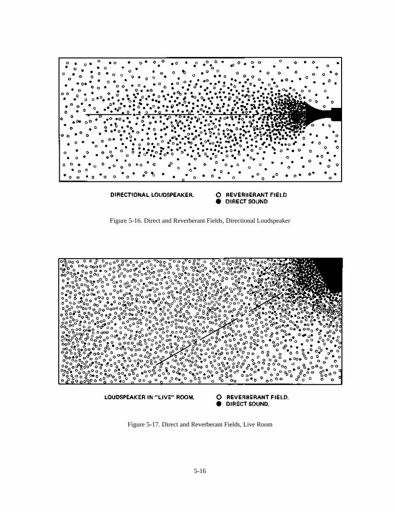
Figure 5-16. Direct and Reverberant Fields, Directional Loudspeaker

Figure 5-17. Direct and Reverberant Fields, Live Room

5-16

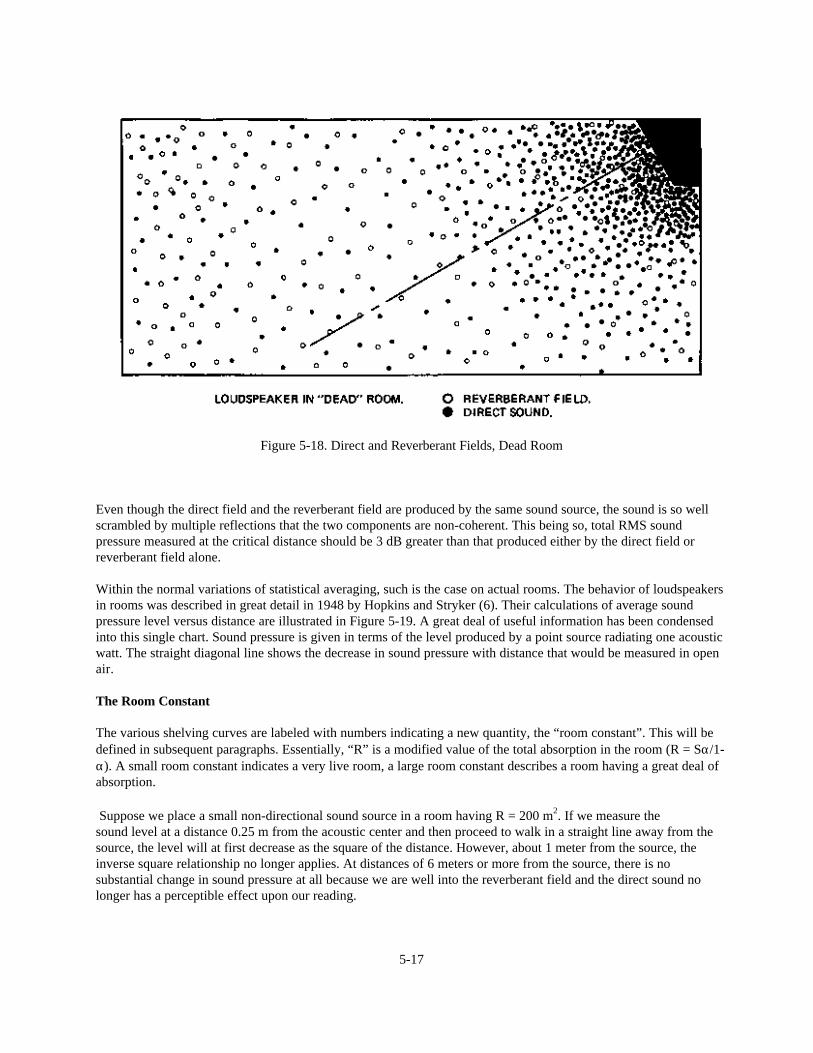
Figure 5-18. Direct and Reverberant Fields, Dead Room

Even though the direct field and the reverberant field are produced by the same sound source, the sound is so wellscrambled by multiple reflections that the two components are non-coherent. This being so, total RMS soundpressure measured at the critical distance should be 3 dB greater than that produced either by the direct field orreverberant field alone.

Within the normal variations of statistical averaging, such is the case on actual rooms. The behavior of loudspeakersin rooms was described in great detail in 1948 by Hopkins and Stryker (6). Their calculations of average soundpressure level versus distance are illustrated in Figure 5-19. A great deal of useful information has been condensedinto this single chart. Sound pressure is given in terms of the level produced by a point source radiating one acousticwatt. The straight diagonal line shows the decrease in sound pressure with distance that would be measured in openair.

The Room Constant

The various shelving curves are labeled with numbers indicating a new quantity, the “room constant”. This will bedefined in subsequent paragraphs. Essentially, “R” is a modified value of the total absorption in the room (R = Sα/1-α). A small room constant indicates a very live room, a large room constant describes a room having a great deal ofabsorption.

Suppose we place a small non-directional sound source in a room having R = 200 m2. If we measure thesound level at a distance 0.25 m from the acoustic center and then proceed to walk in a straight line away from thesource, the level will at first decrease as the square of the distance. However, about 1 meter from the source, theinverse square relationship no longer applies. At distances of 6 meters or more from the source, there is nosubstantial change in sound pressure at all because we are well into the reverberant field and the direct sound nolonger has a perceptible effect upon our reading.

5-17

Figure 5-19. SPL (Point Source Radiating One Acoustic Watt)vs. R and Distance from Source

If we reverse our path and walk back toward the source from a distance of 12 or 15 meters, sound pressure at firstremains unchanged and then gradually begins to climb until, at a distance about 2 meters from the source, it hasincreased 3 dB above the reverberant field reading. This position, indicated by the mark on the curve, is the criticaldistance.

The chart of Figure 5-20 is a universal relationship in which critical distance is used as the measuring stick. It can beseem that the effective transition zone from the reverberant field to the direct field exists over a range from aboutone-half the critical distance to about twice the critical distance. At one-half the critical distance, the total soundfield is 1 dB greater than the direct field alone; at twice the critical distance, the total sound field is 1 dB greater thanthe reverberant field alone.

The ratio of direct to reverberant sound can be calculated from the simple equation shown below the chart, orestimated directly from the chart itself. For example, at four times Dc the direct sound field is 12 dB less than thereverberant sound field. At one-half Dc, the direct sound field is 6 dB greater than the reverberant sound field.

Remember that although critical distance depends on the directivity of the source and the absorption characteristicsof the room, the relationships expressed in Figure 5-19 remain unchanged. Once Dc is known, all other factors canbe calculated without regard to room characteristics. With a directional sound source, however, a given set ofcalculations can be used only along a specified axis. On any other axis the critical distance will change and must berecalculated.

Let us investigate these two factors in some detail: first the room constant R, and then the directivity factor.

5-18

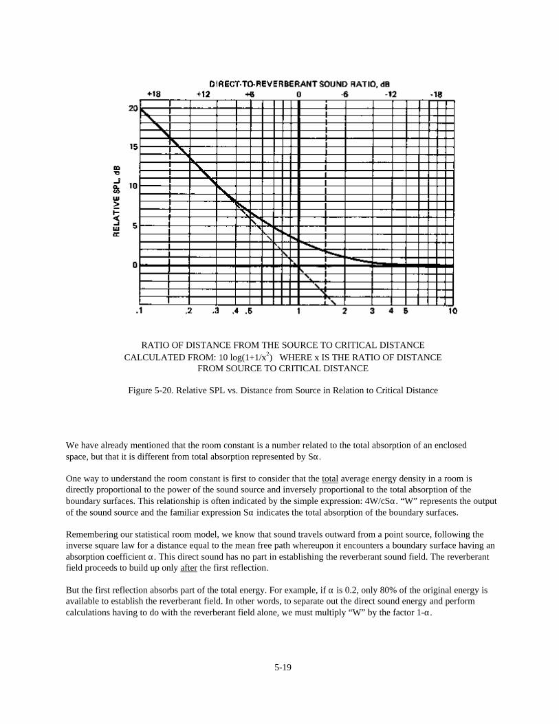
RATIO OF DISTANCE FROM THE SOURCE TO CRITICAL DISTANCECALCULATED FROM: 10 log(1+1/x2) WHERE x IS THE RATIO OF DISTANCE

FROM SOURCE TO CRITICAL DISTANCE

Figure 5-20. Relative SPL vs. Distance from Source in Relation to Critical Distance

We have already mentioned that the room constant is a number related to the total absorption of an enclosedspace, but that it is different from total absorption represented by Sα.

One way to understand the room constant is first to consider that the total average energy density in a room isdirectly proportional to the power of the sound source and inversely proportional to the total absorption of theboundary surfaces. This relationship is often indicated by the simple expression: 4W/cSα. “W” represents the outputof the sound source and the familiar expression Sα indicates the total absorption of the boundary surfaces.

Remembering our statistical room model, we know that sound travels outward from a point source, following theinverse square law for a distance equal to the mean free path whereupon it encounters a boundary surface having anabsorption coefficient α. This direct sound has no part in establishing the reverberant sound field. The reverberantfield proceeds to build up only after the first reflection.

But the first reflection absorbs part of the total energy. For example, if α is 0.2, only 80% of the original energy isavailable to establish the reverberant field. In other words, to separate out the direct sound energy and performcalculations having to do with the reverberant field alone, we must multiply “W” by the factor 1-α.

5-19

This results in the equation:

Erev = 4W/cR *

This gives the average energy density of the reverberant field alone.becomes

Erev = 4W(1-α)/cSα

If we let “R” equal S/1-α, the equation

Note that the equation has nothing to do with the directivity of the sound source. From previous examples, we knowthat the directivity of the source affects critical distance and the contour of the boundary zone. But power is power,and it would seem to make no difference whether one acoustic watt is radiated in all directions from a point source orconcentrated by a highly directional horn.

Is this really true? The equation assumes that the proportion of energy left after the first reflection is equivalent toW(1-α). Suppose we have a room in which part of the absorption is supplied by an open window. Our sound sourceis a highly directional horn located near the window. According to the equation the energy density of the reverberantfield will be exactly the same whether the horn is pointed into the room or out of the window! This obviously isfallacious, and is a good example of the importance of understanding the basis for acoustical equations instead ofmerely plugging in numbers.

*With room dimensions in meters and acoustic power in watts, the reverberant field level in dB isLrev = 10 log W/R -F 126 dB. See Figure 5-21.

Figure 5-21. Steady-State Reverberant Field SPL vs. Acoustic Power and Room Constant

5-20

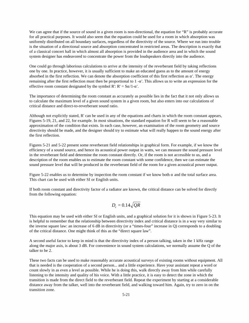
We can agree that if the source of sound in a given room is non-directional, the equation for “R” is probably accuratefor all practical purposes. It would also seem that the equation could be used for a room in which absorption wasuniformly distributed on all boundary surfaces, regardless of the directivity of the source. Where we run into troubleis the situation of a directional source and absorption concentrated in restricted areas. The description is exactly thatof a classical concert hall in which almost all absorption is provided in the audience area and in which the soundsystem designer has endeavored to concentrate the power from the loudspeakers directly into the audience.

One could go through laborious calculations to arrive at the intensity of the reverberant field by taking reflectionsone by one. In practice, however, it is usually sufficient to make an educated guess as to the amount of energyabsorbed in the first reflection. We can denote the absorption coefficient of this first reflection as α'. The energyremaining after the first reflection must then be proportional to 1 -α'. This allows us to write an expression for theeffective room constant designated by the symbol R': R' = Sα/1-α'.

The importance of determining the room constant as accurately as possible lies in the fact that it not only allows usto calculate the maximum level of a given sound system in a given room, but also enters into our calculations ofcritical distance and direct-to-reverberant sound ratio.

Although not explicitly stated, R' can be used in any of the equations and charts in which the room constant appears,Figures 5-19, 21, and 22, for example. In most situations, the standard equation for R will seem to be a reasonableapproximation of the condition that exists. In each case, however, an examination of the room geometry and sourcedirectivity should be made, and the designer should try to estimate what will really happen to the sound energy afterthe first reflection.

Figures 5-21 and 5-22 present some reverberant field relationships in graphical form. For example, if we know theefficiency of a sound source, and hence its acoustical power output in watts, we can measure the sound pressure levelin the reverberant field and determine the room constant directly. Or, if the room is not accessible to us, and adescription of the room enables us to estimate the room constant with some confidence, then we can estimate thesound pressure level that will be produced in the reverberant field of the room for a given acoustical power output.

Figure 5-22 enables us to determine by inspection the room constant if we know both α and the total surface area.This chart can be used with either SI or English units.

If both room constant and directivity factor of a radiator are known, the critical distance can be solved for directlyfrom the following equation:

D QRc = 0 14.

This equation may be used with either SI or English units, and a graphical solution for it is shown in Figure 5-23. Itis helpful to remember that the relationship between directivity index and critical distance is in a way very similar tothe inverse square law: an increase of 6 dB in directivity (or a “times-four” increase in Q) corresponds to a doublingof the critical distance. One might think of this as the “direct square law”.

A second useful factor to keep in mind is that the directivity index of a person talking, taken in the 1 kHz rangealong the major axis, is about 3 dB. For convenience in sound system calculations, we normally assume the Q of thetalker to be 2.

These two facts can be used to make reasonably accurate acoustical surveys of existing rooms without equipment. Allthat is needed is the cooperation of a second person... and a little experience. Have your assistant repeat a word orcount slowly in as even a level as possible. While he is doing this, walk directly away from him while carefullylistening to the intensity and quality of his voice. With a little practice, it is easy to detect the zone in which thetransition is made from the direct field to the reverberant field. Repeat the experiment by starting at a considerabledistance away from the talker, well into the reverberant field, and walking toward him. Again, try to zero in on thetransition zone.

5-21

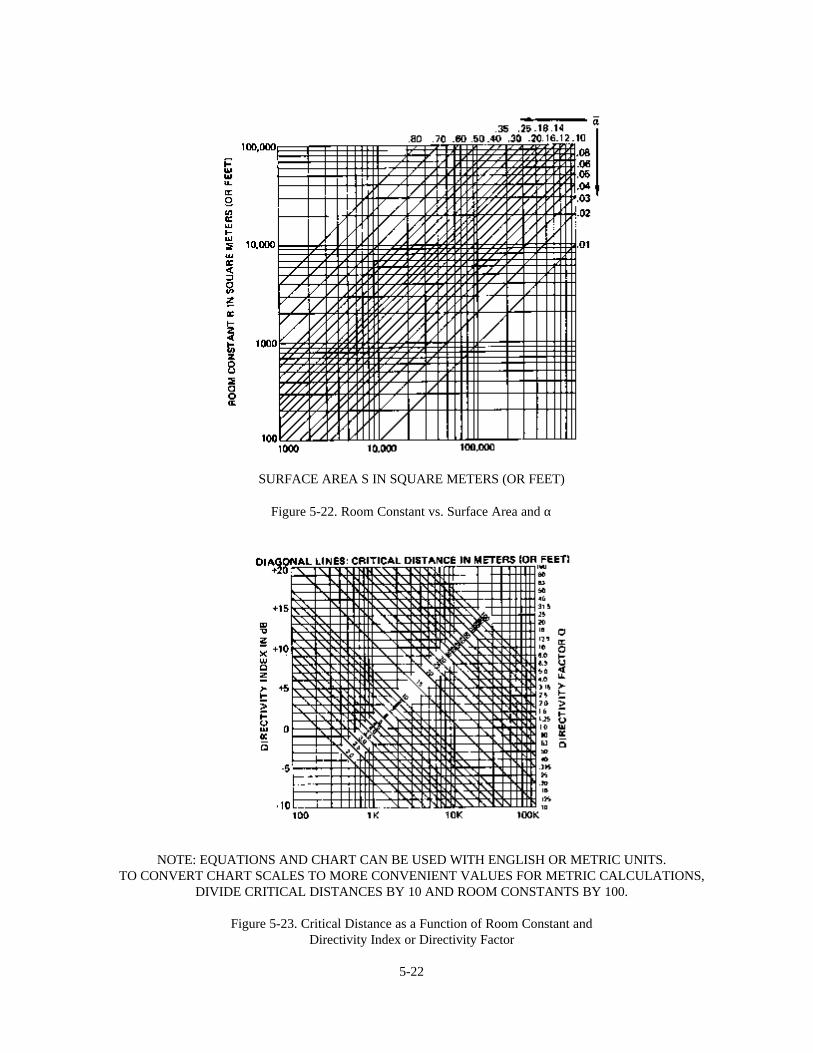
SURFACE AREA S IN SQUARE METERS (OR FEET)

Figure 5-22. Room Constant vs. Surface Area and α

NOTE: EQUATIONS AND CHART CAN BE USED WITH ENGLISH OR METRIC UNITS.TO CONVERT CHART SCALES TO MORE CONVENIENT VALUES FOR METRIC CALCULATIONS,

DIVIDE CRITICAL DISTANCES BY 10 AND ROOM CONSTANTS BY 100.

Figure 5-23. Critical Distance as a Function of Room Constant andDirectivity Index or Directivity Factor

5-22

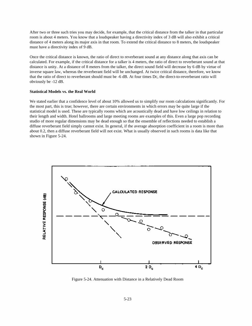
After two or three such tries you may decide, for example, that the critical distance from the talker in that particularroom is about 4 meters. You know that a loudspeaker having a directivity index of 3 dB will also exhibit a criticaldistance of 4 meters along its major axis in that room. To extend the critical distance to 8 meters, the loudspeakermust have a directivity index of 9 dB.

Once the critical distance is known, the ratio of direct to reverberant sound at any distance along that axis can becalculated. For example, if the critical distance for a talker is 4 meters, the ratio of direct to reverberant sound at thatdistance is unity. At a distance of 8 meters from the talker, the direct sound field will decrease by 6 dB by virtue ofinverse square law, whereas the reverberant field will be unchanged. At twice critical distance, therefore, we knowthat the ratio of direct to reverberant should must be -6 dB. At four times Dc, the direct-to-reverberant ratio willobviously be -12 dB.

Statistical Models vs. the Real World

We stated earlier that a confidence level of about 10% allowed us to simplify our room calculations significantly. Forthe most part, this is true; however, there are certain environments in which errors may be quite large if thestatistical model is used. These are typically rooms which are acoustically dead and have low ceilings in relation totheir length and width. Hotel ballrooms and large meeting rooms are examples of this. Even a large pop recordingstudio of more regular dimensions may be dead enough so that the ensemble of reflections needed to establish adiffuse reverberant field simply cannot exist. In general, if the average absorption coefficient in a room is more thanabout 0.2, then a diffuse reverberant field will not exist. What is usually observed in such rooms is data like thatshown in Figure 5-24.

Figure 5-24. Attenuation with Distance in a Relatively Dead Room

5-23

Peutz (9) has developed an empirical equation which will enable a designer to estimate the approximate slope of theattenuation curve beyond Dc in rooms with relatively low ceilings and low reverberation times:

∆ ≈ 0 4

60

. VhT

dB

In this equation, ∆ represents the additional fall-off in level in dB per doubling of distance beyond Dc. V isthe volume in meters3, h is the ceiling height in meters, and T60 is the reverberation time in seconds. In Englishunits (V in feet3 and h in feet), the equation is:

∆ ≈0 22

60

. VhT

dB

As an example, assume we have a room whose height is 3 meters and whose length and width are 15 and 10meters. Let us assume that the reverberation time is one second. Then:

∆ ≈⋅

=0 4 4503 1

2 8. . dB

Thus, beyond Dc we would observe an additional fall-off of level of about 3 dB per doubling of distance.

5-24

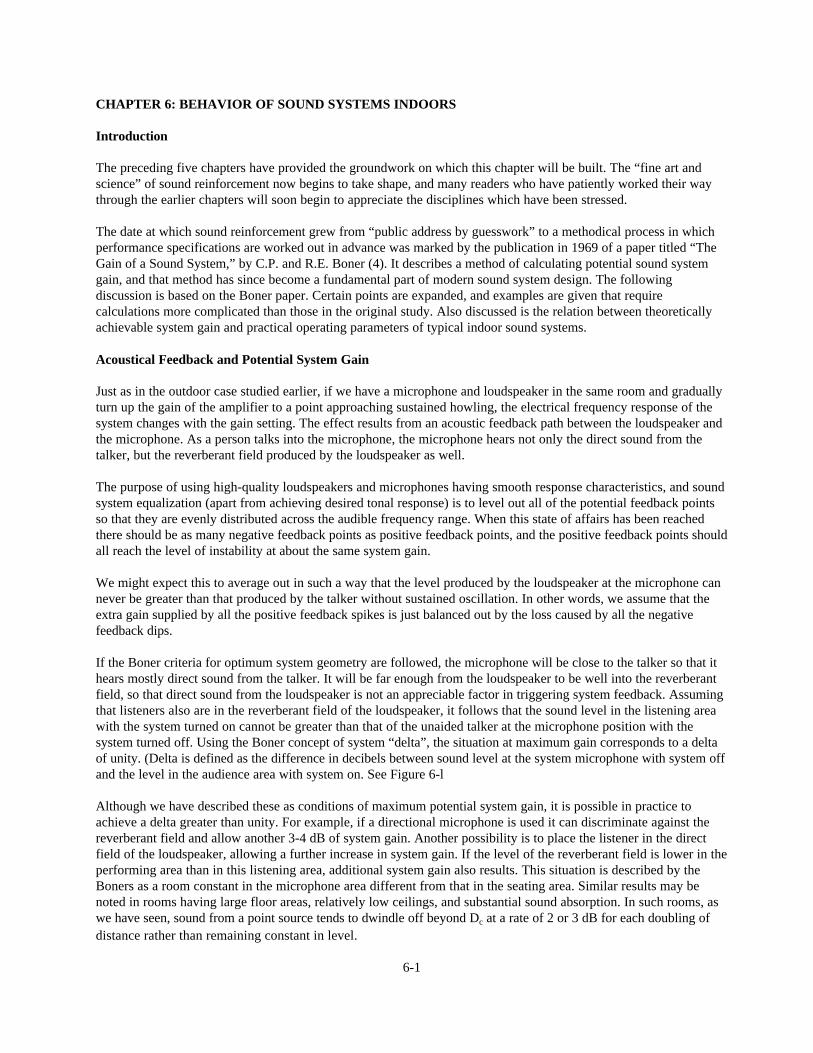
CHAPTER 6: BEHAVIOR OF SOUND SYSTEMS INDOORS

Introduction

The preceding five chapters have provided the groundwork on which this chapter will be built. The “fine art andscience” of sound reinforcement now begins to take shape, and many readers who have patiently worked their waythrough the earlier chapters will soon begin to appreciate the disciplines which have been stressed.

The date at which sound reinforcement grew from “public address by guesswork” to a methodical process in whichperformance specifications are worked out in advance was marked by the publication in 1969 of a paper titled “TheGain of a Sound System,” by C.P. and R.E. Boner (4). It describes a method of calculating potential sound systemgain, and that method has since become a fundamental part of modern sound system design. The followingdiscussion is based on the Boner paper. Certain points are expanded, and examples are given that requirecalculations more complicated than those in the original study. Also discussed is the relation between theoreticallyachievable system gain and practical operating parameters of typical indoor sound systems.

Acoustical Feedback and Potential System Gain

Just as in the outdoor case studied earlier, if we have a microphone and loudspeaker in the same room and graduallyturn up the gain of the amplifier to a point approaching sustained howling, the electrical frequency response of thesystem changes with the gain setting. The effect results from an acoustic feedback path between the loudspeaker andthe microphone. As a person talks into the microphone, the microphone hears not only the direct sound from thetalker, but the reverberant field produced by the loudspeaker as well.

The purpose of using high-quality loudspeakers and microphones having smooth response characteristics, and soundsystem equalization (apart from achieving desired tonal response) is to level out all of the potential feedback pointsso that they are evenly distributed across the audible frequency range. When this state of affairs has been reachedthere should be as many negative feedback points as positive feedback points, and the positive feedback points shouldall reach the level of instability at about the same system gain.

We might expect this to average out in such a way that the level produced by the loudspeaker at the microphone cannever be greater than that produced by the talker without sustained oscillation. In other words, we assume that theextra gain supplied by all the positive feedback spikes is just balanced out by the loss caused by all the negativefeedback dips.

If the Boner criteria for optimum system geometry are followed, the microphone will be close to the talker so that ithears mostly direct sound from the talker. It will be far enough from the loudspeaker to be well into the reverberantfield, so that direct sound from the loudspeaker is not an appreciable factor in triggering system feedback. Assumingthat listeners also are in the reverberant field of the loudspeaker, it follows that the sound level in the listening areawith the system turned on cannot be greater than that of the unaided talker at the microphone position with thesystem turned off. Using the Boner concept of system “delta”, the situation at maximum gain corresponds to a deltaof unity. (Delta is defined as the difference in decibels between sound level at the system microphone with system offand the level in the audience area with system on. See Figure 6-l

Although we have described these as conditions of maximum potential system gain, it is possible in practice toachieve a delta greater than unity. For example, if a directional microphone is used it can discriminate against thereverberant field and allow another 3-4 dB of system gain. Another possibility is to place the listener in the directfield of the loudspeaker, allowing a further increase in system gain. If the level of the reverberant field is lower in theperforming area than in this listening area, additional system gain also results. This situation is described by theBoners as a room constant in the microphone area different from that in the seating area. Similar results may benoted in rooms having large floor areas, relatively low ceilings, and substantial sound absorption. In such rooms, aswe have seen, sound from a point source tends to dwindle off beyond Dc at a rate of 2 or 3 dB for each doubling ofdistance rather than remaining constant in level.

6-1

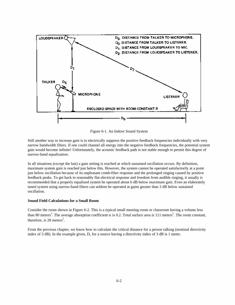
Figure 6-1. An Indoor Sound System

Still another way to increase gain is to electrically suppress the positive feedback frequencies individually with verynarrow bandwidth filters. If one could channel all energy into the negative feedback frequencies, the potential systemgain would become infinite! Unfortunately, the acoustic feedback path is not stable enough to permit this degree ofnarrow-band equalization.

In all situations (except the last) a gain setting is reached at which sustained oscillation occurs. By definition,maximum system gain is reached just below this. However, the system cannot be operated satisfactorily at a pointjust below oscillation because of its unpleasant comb-filter response and the prolonged ringing caused by positivefeedback peaks. To get back to reasonably flat electrical response and freedom from audible ringing, it usually isrecommended that a properly equalized system be operated about 6 dB below maximum gain. Even an elaboratelytuned system using narrow-band filters can seldom be operated at gains greater than 3 dB below sustainedoscillation.

Sound Field Calculations for a Small Room

Consider the room shown in Figure 6-2. This is a typical small meeting room or classroom having a volume lessthan 80 meters3. The average absorption coefficient α is 0.2. Total surface area is 111 meters2. The room constant,therefore, is 28 meters2.

From the previous chapter, we know how to calculate the critical distance for a person talking (nominal directivityindex of 3 dB). In the example given, Dc for a source having a directivity index of 3 dB is 1 meter.

6-2

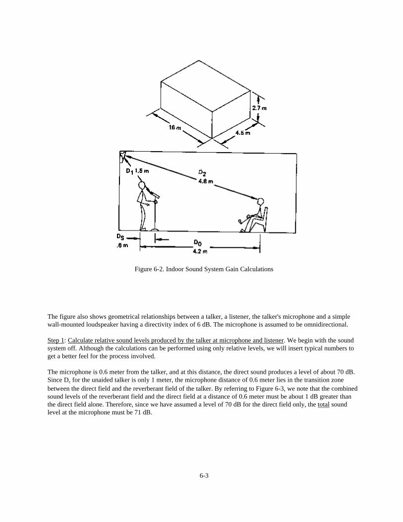
Figure 6-2. Indoor Sound System Gain Calculations

The figure also shows geometrical relationships between a talker, a listener, the talker's microphone and a simplewall-mounted loudspeaker having a directivity index of 6 dB. The microphone is assumed to be omnidirectional.

Step 1: Calculate relative sound levels produced by the talker at microphone and listener. We begin with the soundsystem off. Although the calculations can be performed using only relative levels, we will insert typical numbers toget a better feel for the process involved.

The microphone is 0.6 meter from the talker, and at this distance, the direct sound produces a level of about 70 dB.Since Dc for the unaided talker is only 1 meter, the microphone distance of 0.6 meter lies in the transition zonebetween the direct field and the reverberant field of the talker. By referring to Figure 6-3, we note that the combinedsound levels of the reverberant field and the direct field at a distance of 0.6 meter must be about 1 dB greater thanthe direct field alone. Therefore, since we have assumed a level of 70 dB for the direct field only, the total soundlevel at the microphone must be 71 dB.

6-3

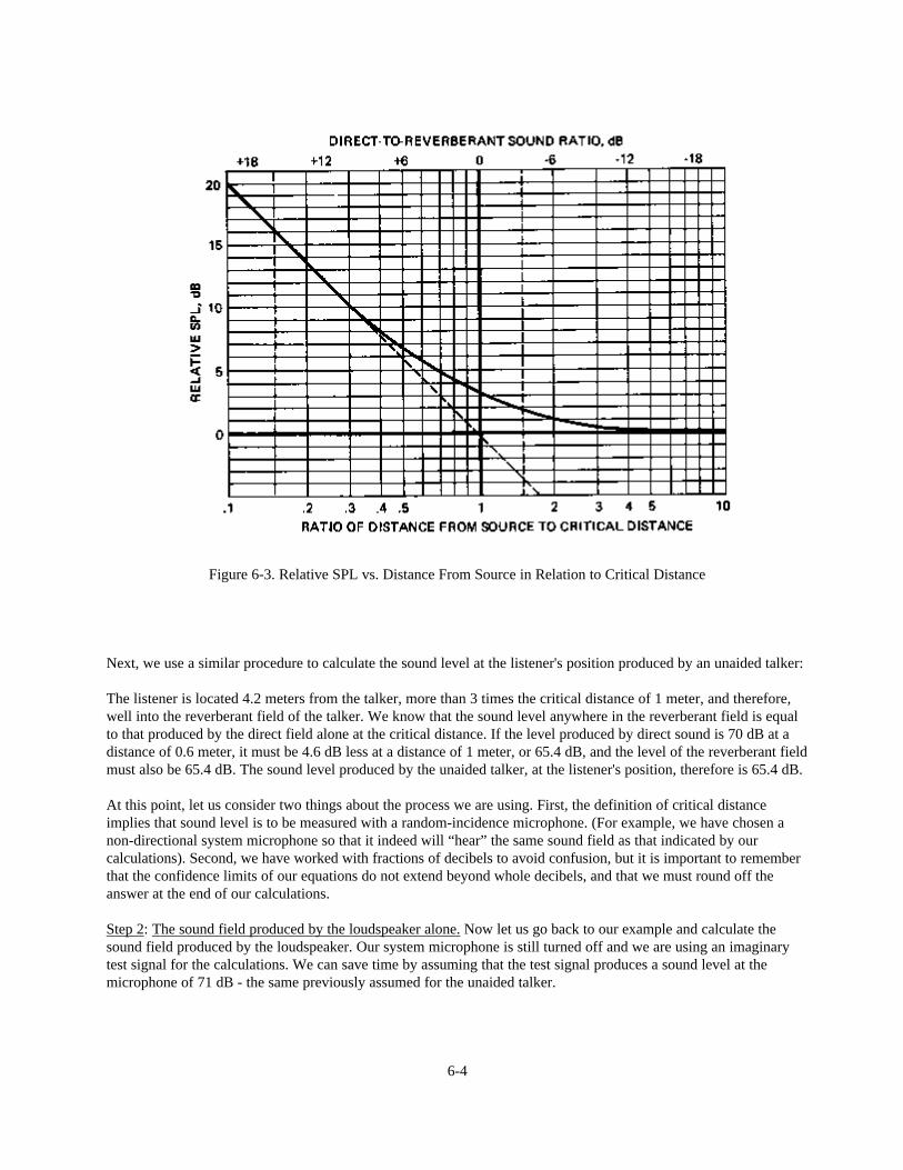
Figure 6-3. Relative SPL vs. Distance From Source in Relation to Critical Distance

Next, we use a similar procedure to calculate the sound level at the listener's position produced by an unaided talker:

The listener is located 4.2 meters from the talker, more than 3 times the critical distance of 1 meter, and therefore,well into the reverberant field of the talker. We know that the sound level anywhere in the reverberant field is equalto that produced by the direct field alone at the critical distance. If the level produced by direct sound is 70 dB at adistance of 0.6 meter, it must be 4.6 dB less at a distance of 1 meter, or 65.4 dB, and the level of the reverberant fieldmust also be 65.4 dB. The sound level produced by the unaided talker, at the listener's position, therefore is 65.4 dB.

At this point, let us consider two things about the process we are using. First, the definition of critical distanceimplies that sound level is to be measured with a random-incidence microphone. (For example, we have chosen anon-directional system microphone so that it indeed will “hear” the same sound field as that indicated by ourcalculations). Second, we have worked with fractions of decibels to avoid confusion, but it is important to rememberthat the confidence limits of our equations do not extend beyond whole decibels, and that we must round off theanswer at the end of our calculations.

Step 2: The sound field produced by the loudspeaker alone. Now let us go back to our example and calculate thesound field produced by the loudspeaker. Our system microphone is still turned off and we are using an imaginarytest signal for the calculations. We can save time by assuming that the test signal produces a sound level at themicrophone of 71 dB - the same previously assumed for the unaided talker.

6-4

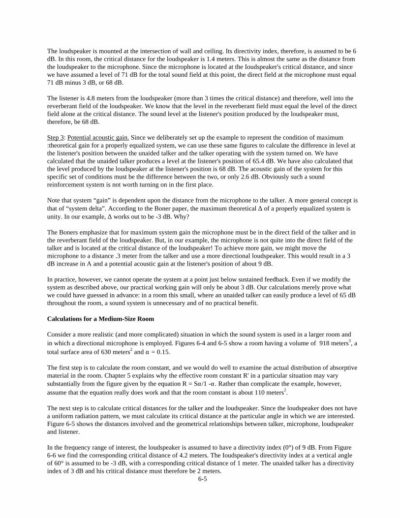
The loudspeaker is mounted at the intersection of wall and ceiling. Its directivity index, therefore, is assumed to be 6dB. In this room, the critical distance for the loudspeaker is 1.4 meters. This is almost the same as the distance fromthe loudspeaker to the microphone. Since the microphone is located at the Ioudspeaker's critical distance, and sincewe have assumed a level of 71 dB for the total sound field at this point, the direct field at the microphone must equal71 dB minus 3 dB, or 68 dB.

The listener is 4.8 meters from the loudspeaker (more than 3 times the critical distance) and therefore, well into thereverberant field of the loudspeaker. We know that the level in the reverberant field must equal the level of the directfield alone at the critical distance. The sound level at the listener's position produced by the loudspeaker must,therefore, be 68 dB.

Step 3: Potential acoustic gain. Since we deliberately set up the example to represent the condition of maximum:theoretical gain for a properly equalized system, we can use these same figures to calculate the difference in level atthe listener's position between the unaided talker and the talker operating with the system turned on. We havecalculated that the unaided talker produces a level at the listener's position of 65.4 dB. We have also calculated thatthe level produced by the loudspeaker at the listener's position is 68 dB. The acoustic gain of the system for thisspecific set of conditions must be the difference between the two, or only 2.6 dB. Obviously such a soundreinforcement system is not worth turning on in the first place.

Note that system “gain” is dependent upon the distance from the microphone to the talker. A more general concept isthat of “system delta”. According to the Boner paper, the maximum theoretical ∆ of a properly equalized system isunity. In our example, ∆ works out to be -3 dB. Why?

The Boners emphasize that for maximum system gain the microphone must be in the direct field of the talker and inthe reverberant field of the loudspeaker. But, in our example, the microphone is not quite into the direct field of thetalker and is located at the critical distance of the loudspeaker! To achieve more gain, we might move themicrophone to a distance .3 meter from the talker and use a more directional loudspeaker. This would result in a 3dB increase in A and a potential acoustic gain at the listener's position of about 9 dB.

In practice, however, we cannot operate the system at a point just below sustained feedback. Even if we modify thesystem as described above, our practical working gain will only be about 3 dB. Our calculations merely prove whatwe could have guessed in advance: in a room this small, where an unaided talker can easily produce a level of 65 dBthroughout the room, a sound system is unnecessary and of no practical benefit.

Calculations for a Medium-Size Room

Consider a more realistic (and more complicated) situation in which the sound system is used in a larger room andin which a directional microphone is employed. Figures 6-4 and 6-5 show a room having a volume of 918 meters3, atotal surface area of 630 meters2 and α = 0.15.

The first step is to calculate the room constant, and we would do well to examine the actual distribution of absorptivematerial in the room. Chapter 5 explains why the effective room constant R' in a particular situation may varysubstantially from the figure given by the equation R = Sα/1 -α. Rather than complicate the example, however,assume that the equation really does work and that the room constant is about 110 meters2.

The next step is to calculate critical distances for the talker and the loudspeaker. Since the loudspeaker does not havea uniform radiation pattern, we must calculate its critical distance at the particular angle in which we are interested.Figure 6-5 shows the distances involved and the geometrical relationships between talker, microphone, loudspeakerand listener.

In the frequency range of interest, the loudspeaker is assumed to have a directivity index (0°) of 9 dB. From Figure6-6 we find the corresponding critical distance of 4.2 meters. The Ioudspeaker's directivity index at a vertical angleof 60° is assumed to be -3 dB, with a corresponding critical distance of 1 meter. The unaided talker has a directivityindex of 3 dB and his critical distance must therefore be 2 meters.

6-5

Figure 6-4. A Sound System in a Medium-Size Room

Figure 6-5. Sound System in a Medium-Size Room, Gain Calculations

6-6

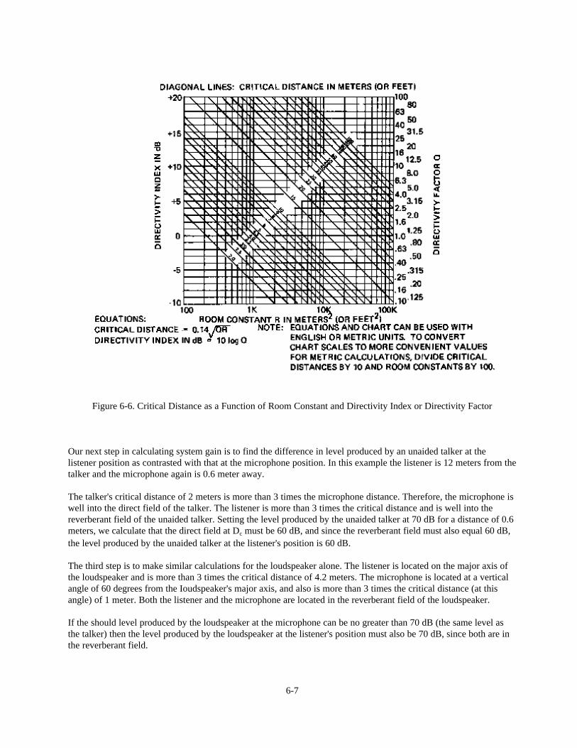
Figure 6-6. Critical Distance as a Function of Room Constant and Directivity Index or Directivity Factor

Our next step in calculating system gain is to find the difference in level produced by an unaided talker at thelistener position as contrasted with that at the microphone position. In this example the listener is 12 meters from thetalker and the microphone again is 0.6 meter away.

The talker's critical distance of 2 meters is more than 3 times the microphone distance. Therefore, the microphone iswell into the direct field of the talker. The listener is more than 3 times the critical distance and is well into thereverberant field of the unaided talker. Setting the level produced by the unaided talker at 70 dB for a distance of 0.6meters, we calculate that the direct field at Dc must be 60 dB, and since the reverberant field must also equal 60 dB,the level produced by the unaided talker at the listener's position is 60 dB.

The third step is to make similar calculations for the loudspeaker alone. The listener is located on the major axis ofthe loudspeaker and is more than 3 times the critical distance of 4.2 meters. The microphone is located at a verticalangle of 60 degrees from the Ioudspeaker's major axis, and also is more than 3 times the critical distance (at thisangle) of 1 meter. Both the listener and the microphone are located in the reverberant field of the loudspeaker.

If the should level produced by the loudspeaker at the microphone can be no greater than 70 dB (the same level asthe talker) then the level produced by the loudspeaker at the listener's position must also be 70 dB, since both are inthe reverberant field.

6-7

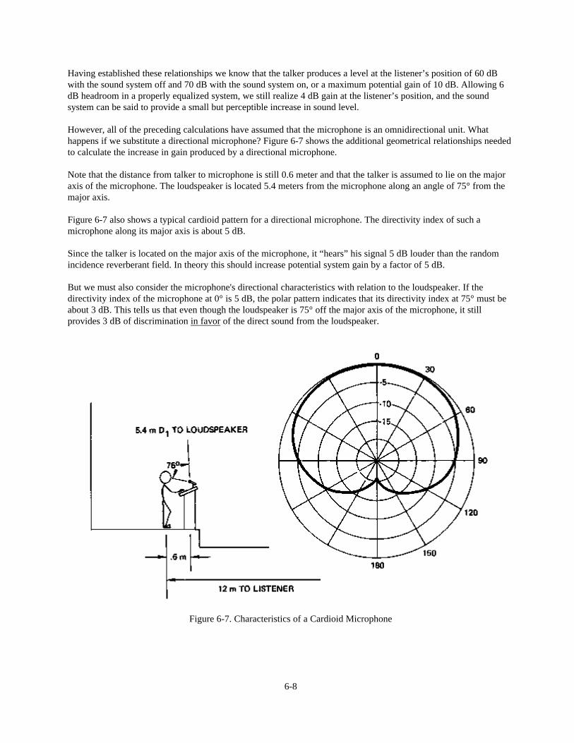
Having established these relationships we know that the talker produces a level at the listener’s position of 60 dBwith the sound system off and 70 dB with the sound system on, or a maximum potential gain of 10 dB. Allowing 6dB headroom in a properly equalized system, we still realize 4 dB gain at the listener’s position, and the soundsystem can be said to provide a small but perceptible increase in sound level.

However, all of the preceding calculations have assumed that the microphone is an omnidirectional unit. Whathappens if we substitute a directional microphone? Figure 6-7 shows the additional geometrical relationships neededto calculate the increase in gain produced by a directional microphone.

Note that the distance from talker to microphone is still 0.6 meter and that the talker is assumed to lie on the majoraxis of the microphone. The loudspeaker is located 5.4 meters from the microphone along an angle of 75° from themajor axis.

Figure 6-7 also shows a typical cardioid pattern for a directional microphone. The directivity index of such amicrophone along its major axis is about 5 dB.

Since the talker is located on the major axis of the microphone, it “hears” his signal 5 dB louder than the randomincidence reverberant field. In theory this should increase potential system gain by a factor of 5 dB.

But we must also consider the microphone's directional characteristics with relation to the loudspeaker. If thedirectivity index of the microphone at 0° is 5 dB, the polar pattern indicates that its directivity index at 75° must beabout 3 dB. This tells us that even though the loudspeaker is 75° off the major axis of the microphone, it stillprovides 3 dB of discrimination in favor of the direct sound from the loudspeaker.

Figure 6-7. Characteristics of a Cardioid Microphone

6-8

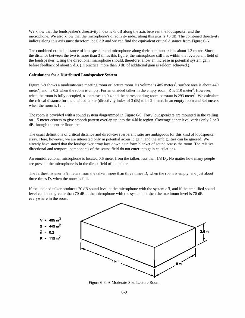
We know that the Ioudspeaker's directivity index is -3 dB along the axis between the loudspeaker and themicrophone. We also know that the microphone's directivity index along this axis is +3 dB. The combined directivityindices along this axis must therefore, be 0 dB and we can find the equivalent critical distance from Figure 6-6.

The combined critical distance of loudspeaker and microphone along their common axis is about 1.3 meter. Sincethe distance between the two is more than 3 times this figure, the microphone still lies within the reverberant field ofthe loudspeaker. Using the directional microphone should, therefore, allow an increase in potential system gainbefore feedback of about 5 dB. (In practice, more than 3 dB of additional gain is seldom achieved.)

Calculations for a Distributed Loudspeaker System

Figure 6-8 shows a moderate-size meeting room or lecture room. Its volume is 485 meters3, surface area is about 440meter2, and is 0.2 when the room is empty. For an unaided talker in the empty room, R is 110 meter2. However,when the room is fully occupied, α increases to 0.4 and the corresponding room constant is 293 meter2. We calculatethe critical distance for the unaided talker (directivity index of 3 dB) to be 2 meters in an empty room and 3.4 meterswhen the room is full.

The room is provided with a sound system diagrammed in Figure 6-9. Forty loudspeakers are mounted in the ceilingon 1.5 meter centers to give smooth pattern overlap up into the 4-kHz region. Coverage at ear level varies only 2 or 3dB through the entire floor area.

The usual definitions of critical distance and direct-to-reverberant ratio are ambiguous for this kind of loudspeakerarray. Here, however, we are interested only in potential acoustic gain, and the ambiguities can be ignored. Wealready have stated that the loudspeaker array lays down a uniform blanket of sound across the room. The relativedirectional and temporal components of the sound field do not enter into gain calculations.

An omnidirectional microphone is located 0.6 meter from the talker, less than 1/3 Dc. No matter how many peopleare present, the microphone is in the direct field of the talker.

The farthest listener is 9 meters from the talker, more than three times Dc when the room is empty, and just aboutthree times Dc when the room is full.

If the unaided talker produces 70 dB sound level at the microphone with the system off, and if the amplified soundlevel can be no greater than 70 dB at the microphone with the system on, then the maximum level is 70 dBeverywhere in the room.

Figure 6-8. A Moderate-Size Lecture Room

6-9

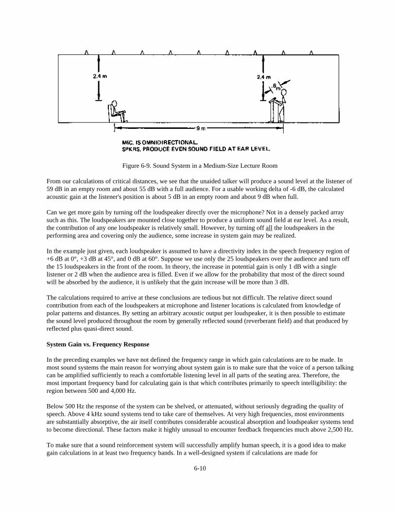
Figure 6-9. Sound System in a Medium-Size Lecture Room

From our calculations of critical distances, we see that the unaided talker will produce a sound level at the listener of59 dB in an empty room and about 55 dB with a full audience. For a usable working delta of -6 dB, the calculatedacoustic gain at the listener's position is about 5 dB in an empty room and about 9 dB when full.

Can we get more gain by turning off the loudspeaker directly over the microphone? Not in a densely packed arraysuch as this. The loudspeakers are mounted close together to produce a uniform sound field at ear level. As a result,the contribution of any one loudspeaker is relatively small. However, by turning off all the loudspeakers in theperforming area and covering only the audience, some increase in system gain may be realized.

In the example just given, each loudspeaker is assumed to have a directivity index in the speech frequency region of+6 dB at 0°, +3 dB at 45°, and 0 dB at 60°. Suppose we use only the 25 loudspeakers over the audience and turn offthe 15 loudspeakers in the front of the room. In theory, the increase in potential gain is only 1 dB with a singlelistener or 2 dB when the audience area is filled. Even if we allow for the probability that most of the direct soundwill be absorbed by the audience, it is unlikely that the gain increase will be more than 3 dB.

The calculations required to arrive at these conclusions are tedious but not difficult. The relative direct soundcontribution from each of the loudspeakers at microphone and listener locations is calculated from knowledge ofpolar patterns and distances. By setting an arbitrary acoustic output per loudspeaker, it is then possible to estimatethe sound level produced throughout the room by generally reflected sound (reverberant field) and that produced byreflected plus quasi-direct sound.

System Gain vs. Frequency Response

In the preceding examples we have not defined the frequency range in which gain calculations are to be made. Inmost sound systems the main reason for worrying about system gain is to make sure that the voice of a person talkingcan be amplified sufficiently to reach a comfortable listening level in all parts of the seating area. Therefore, themost important frequency band for calculating gain is that which contributes primarily to speech intelligibility: theregion between 500 and 4,000 Hz.

Below 500 Hz the response of the system can be shelved, or attenuated, without seriously degrading the quality ofspeech. Above 4 kHz sound systems tend to take care of themselves. At very high frequencies, most environmentsare substantially absorptive, the air itself contributes considerable acoustical absorption and loudspeaker systems tendto become directional. These factors make it highly unusual to encounter feedback frequencies much above 2,500 Hz.

To make sure that a sound reinforcement system will successfully amplify human speech, it is a good idea to makegain calculations in at least two frequency bands. In a well-designed system if calculations are made for

6-10

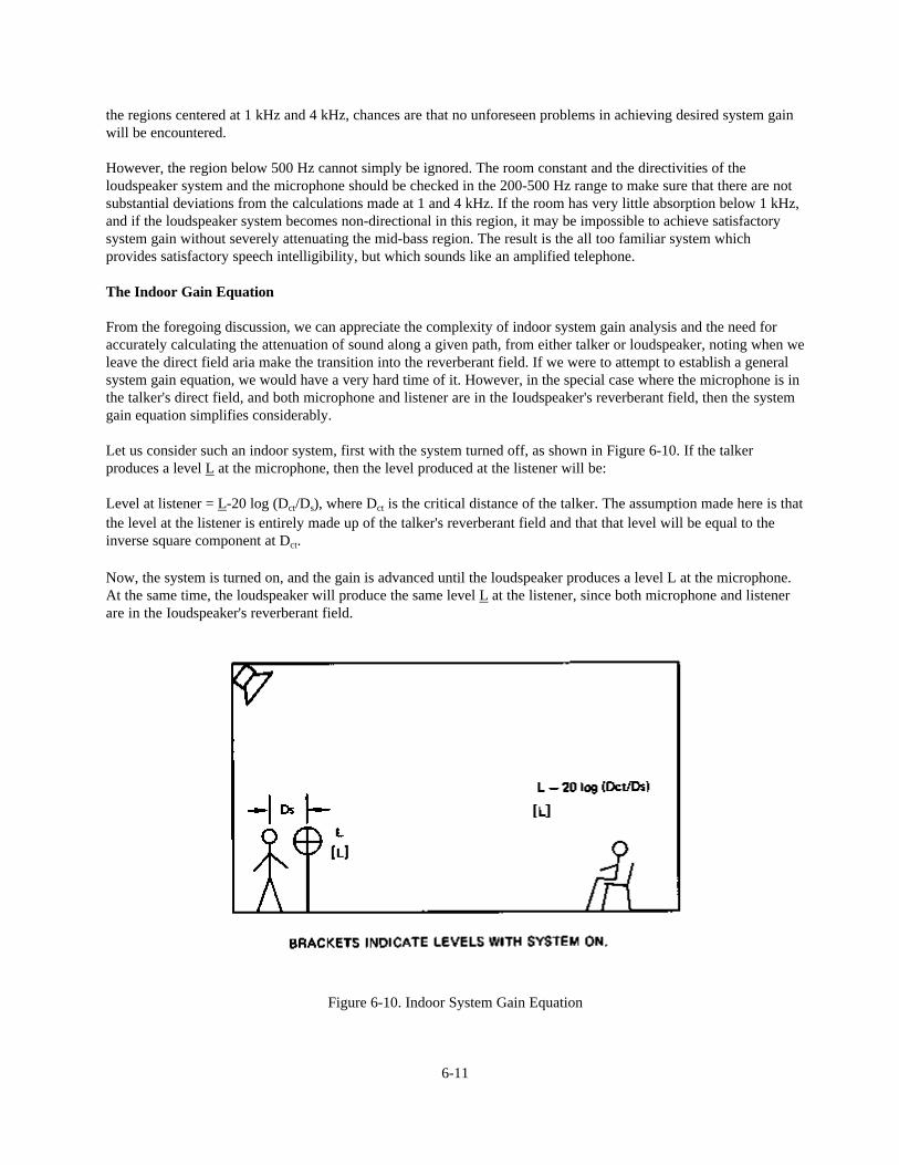
the regions centered at 1 kHz and 4 kHz, chances are that no unforeseen problems in achieving desired system gainwill be encountered.

However, the region below 500 Hz cannot simply be ignored. The room constant and the directivities of theloudspeaker system and the microphone should be checked in the 200-500 Hz range to make sure that there are notsubstantial deviations from the calculations made at 1 and 4 kHz. If the room has very little absorption below 1 kHz,and if the loudspeaker system becomes non-directional in this region, it may be impossible to achieve satisfactorysystem gain without severely attenuating the mid-bass region. The result is the all too familiar system whichprovides satisfactory speech intelligibility, but which sounds like an amplified telephone.

The Indoor Gain Equation

From the foregoing discussion, we can appreciate the complexity of indoor system gain analysis and the need foraccurately calculating the attenuation of sound along a given path, from either talker or loudspeaker, noting when weleave the direct field aria make the transition into the reverberant field. If we were to attempt to establish a generalsystem gain equation, we would have a very hard time of it. However, in the special case where the microphone is inthe talker's direct field, and both microphone and listener are in the Ioudspeaker's reverberant field, then the systemgain equation simplifies considerably.

Let us consider such an indoor system, first with the system turned off, as shown in Figure 6-10. If the talkerproduces a level L at the microphone, then the level produced at the listener will be:

Level at listener = L-20 log (Dct/Ds), where Dct is the critical distance of the talker. The assumption made here is thatthe level at the listener is entirely made up of the talker's reverberant field and that that level will be equal to theinverse square component at Dct.

Now, the system is turned on, and the gain is advanced until the loudspeaker produces a level L at the microphone.At the same time, the loudspeaker will produce the same level L at the listener, since both microphone and listenerare in the Ioudspeaker's reverberant field.

Figure 6-10. Indoor System Gain Equation

6-11

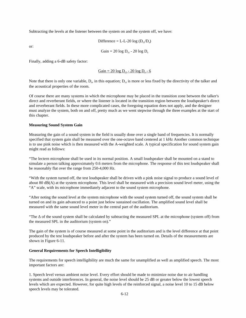
Subtracting the levels at the listener between the system on and the system off, we have:

Difference = L-L-20 log (Dct/Ds)or:

Gain = 20 log Dct - 20 log Ds

Finally, adding a 6-dB safety factor:

Gain = 20 log Dct - 20 log Ds - 6

Note that there is only one variable, Ds, in this equation; Dct is more or less fixed by the directivity of the talker andthe acoustical properties of the room.

Of course there are many systems in which the microphone may be placed in the transition zone between the talker'sdirect and reverberant fields, or where the listener is located in the transition region between the Ioudspeaker's directand reverberant fields. In these more complicated cases, the foregoing equation does not apply, and the designermust analyze the system, both on and off, pretty much as we went stepwise through the three examples at the start ofthis chapter.

Measuring Sound System Gain

Measuring the gain of a sound system in the field is usually done over a single band of frequencies. It is normallyspecified that system gain shall be measured over the one-octave band centered at 1 kHz Another common techniqueis to use pink noise which is then measured with the A-weighted scale. A typical specification for sound system gainmight read as follows:

“The lectern microphone shall be used in its normal position. A small loudspeaker shall be mounted on a stand tosimulate a person talking approximately 0.6 meters from the microphone. The response of this test loudspeaker shallbe reasonably flat over the range from 250-4,000 Hz.

“With the system turned off, the test loudspeaker shall be driven with a pink noise signal to produce a sound level ofabout 80 dB(A) at the system microphone. This level shall be measured with a precision sound level meter, using the“A” scale, with its microphone immediately adjacent to the sound system microphone.

“After noting the sound level at the system microphone with the sound system turned off, the sound system shall beturned on and its gain advanced to a point just below sustained oscillation. The amplified sound level shall bemeasured with the same sound level meter in the central part of the auditorium.

“The ∆ of the sound system shall be calculated by subtracting the measured SPL at the microphone (system off) fromthe measured SPL in the auditorium (system on).”

The gain of the system is of course measured at some point in the auditorium and is the level difference at that pointproduced by the test loudspeaker before and after the system has been turned on. Details of the measurements areshown in Figure 6-11.

General Requirements for Speech Intelligibility

The requirements for speech intelligibility are much the same for unamplified as well as amplified speech. The mostimportant factors are:

1. Speech level versus ambient noise level. Every effort should be made to minimize noise due to air handlingsystems and outside interferences. In general, the noise level should be 25 dB or greater below the lowest speechlevels which are expected. However, for quite high levels of the reinforced signal, a noise level 10 to 15 dB belowspeech levels may be tolerated.

6-12

Figure 6-11. Measurement of Sound System Gain and Delta ()

2. Reverberation time. Speech syllables occur three or four times per second. For reverberation times of 1.5 secondsor less, the effect of reverberant overhang on the clarity of speech will be minimal.

3. Direct-to-reverberant ratio. For reverberation times in excess of 1.5 seconds, the clarity of speech is a function ofboth reverberation time and the ratio of direct-to-reverberant sound.

In an important paper published in the Journal of the Audio Engineering Society (8), Peutz set forth a method ofestimating speech intelligibility which has found considerable application in sound system design. The Peutzfindings were compiled on the basis of data gathered over a period of years. The data and the method used to arriveat the published conclusion are clearly set forth in the paper itself. The conclusions can be summarized as follows:

1. In practice, the articulation loss of consonants can be used as a single indicator of intelligibility. Although theoriginal research of Peutz involved the Dutch language, the findings seem to be equally applicable to English.

2. As would be expected, the researchers found wide variations in both talkers and listeners. However, a 15%articulation loss of consonants seems to be the maximum allowable for acceptable speech intelligibility. In otherwords, if articulation loss of consonants exceeds 15% for the majority of listeners, most of these people will find theintelligibility of speech to be unacceptable.

3. The articulation loss of consonants can be estimated for typical rooms. Articulation loss of consonants is afunction of reverberation time and the direct-to-reverberant sound ratio.

4. As a listener moves farther from a talker (decreasing the direct-to-reverberant sound ratio) articulation loss ofconsonants increases. That is, intelligibility becomes less and less as the direct-to-reverberant ratio decreases.However, this relationship is maintained only to a certain distance, beyond which no further change takes place. Theboundary corresponds to a direct-to-reverberant ratio of -10 dB.

The last point is illustrated graphically in Figure 6-12, adapted from the Peutz paper. Each of the diagonal linescorresponds to a particular reverberation time. Each shelves at a point corresponding to a direct-to-reverberant

6-13

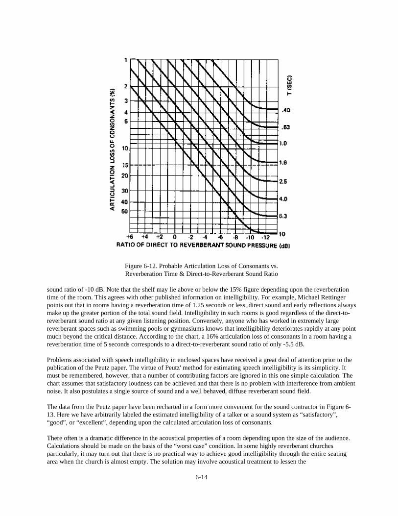
Figure 6-12. Probable Articulation Loss of Consonants vs.Reverberation Time & Direct-to-Reverberant Sound Ratio

sound ratio of -10 dB. Note that the shelf may lie above or below the 15% figure depending upon the reverberationtime of the room. This agrees with other published information on intelligibility. For example, Michael Rettingerpoints out that in rooms having a reverberation time of 1.25 seconds or less, direct sound and early reflections alwaysmake up the greater portion of the total sound field. Intelligibility in such rooms is good regardless of the direct-to-reverberant sound ratio at any given listening position. Conversely, anyone who has worked in extremely largereverberant spaces such as swimming pools or gymnasiums knows that intelligibility deteriorates rapidly at any pointmuch beyond the critical distance. According to the chart, a 16% articulation loss of consonants in a room having areverberation time of 5 seconds corresponds to a direct-to-reverberant sound ratio of only -5.5 dB.

Problems associated with speech intelligibility in enclosed spaces have received a great deal of attention prior to thepublication of the Peutz paper. The virtue of Peutz' method for estimating speech intelligibility is its simplicity. Itmust be remembered, however, that a number of contributing factors are ignored in this one simple calculation. Thechart assumes that satisfactory loudness can be achieved and that there is no problem with interference from ambientnoise. It also postulates a single source of sound and a well behaved, diffuse reverberant sound field.

The data from the Peutz paper have been recharted in a form more convenient for the sound contractor in Figure 6-13. Here we have arbitrarily labeled the estimated intelligibility of a talker or a sound system as “satisfactory”,“good”, or “excellent”, depending upon the calculated articulation loss of consonants.

There often is a dramatic difference in the acoustical properties of a room depending upon the size of the audience.Calculations should be made on the basis of the “worst case” condition. In some highly reverberant churchesparticularly, it may turn out that there is no practical way to achieve good intelligibility through the entire seatingarea when the church is almost empty. The solution may involve acoustical treatment to lessen the

6-14

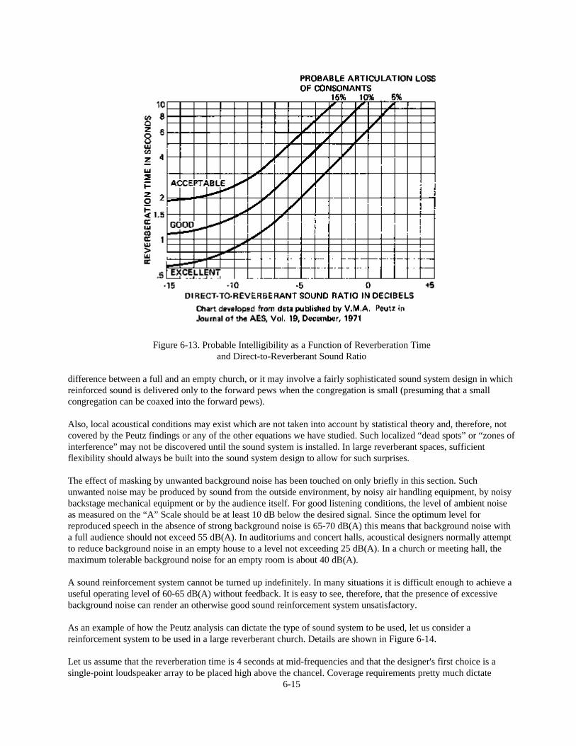
Figure 6-13. Probable Intelligibility as a Function of Reverberation Timeand Direct-to-Reverberant Sound Ratio

difference between a full and an empty church, or it may involve a fairly sophisticated sound system design in whichreinforced sound is delivered only to the forward pews when the congregation is small (presuming that a smallcongregation can be coaxed into the forward pews).

Also, local acoustical conditions may exist which are not taken into account by statistical theory and, therefore, notcovered by the Peutz findings or any of the other equations we have studied. Such localized “dead spots” or “zones ofinterference” may not be discovered until the sound system is installed. In large reverberant spaces, sufficientflexibility should always be built into the sound system design to allow for such surprises.

The effect of masking by unwanted background noise has been touched on only briefly in this section. Suchunwanted noise may be produced by sound from the outside environment, by noisy air handling equipment, by noisybackstage mechanical equipment or by the audience itself. For good listening conditions, the level of ambient noiseas measured on the “A” Scale should be at least 10 dB below the desired signal. Since the optimum level forreproduced speech in the absence of strong background noise is 65-70 dB(A) this means that background noise witha full audience should not exceed 55 dB(A). In auditoriums and concert halls, acoustical designers normally attemptto reduce background noise in an empty house to a level not exceeding 25 dB(A). In a church or meeting hall, themaximum tolerable background noise for an empty room is about 40 dB(A).

A sound reinforcement system cannot be turned up indefinitely. In many situations it is difficult enough to achieve auseful operating level of 60-65 dB(A) without feedback. It is easy to see, therefore, that the presence of excessivebackground noise can render an otherwise good sound reinforcement system unsatisfactory.

As an example of how the Peutz analysis can dictate the type of sound system to be used, let us consider areinforcement system to be used in a large reverberant church. Details are shown in Figure 6-14.

Let us assume that the reverberation time is 4 seconds at mid-frequencies and that the designer's first choice is asingle-point loudspeaker array to be placed high above the chancel. Coverage requirements pretty much dictate

6-15

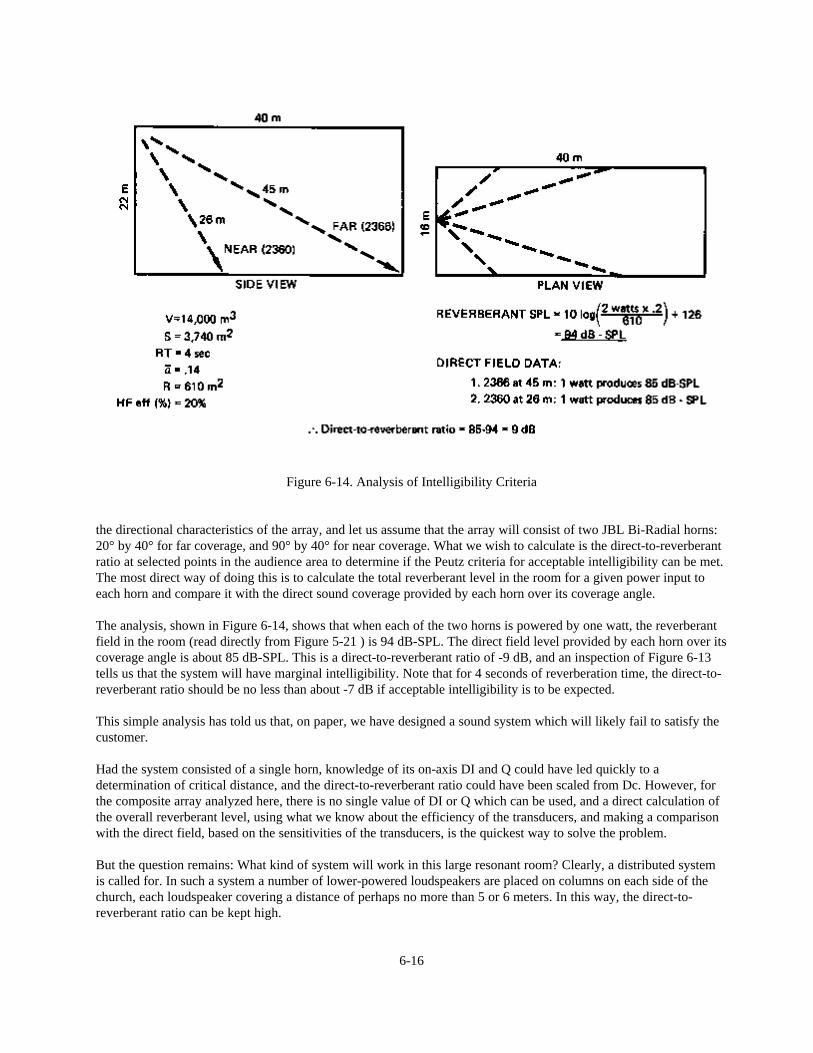
Figure 6-14. Analysis of Intelligibility Criteria

the directional characteristics of the array, and let us assume that the array will consist of two JBL Bi-Radial horns:20° by 40° for far coverage, and 90° by 40° for near coverage. What we wish to calculate is the direct-to-reverberantratio at selected points in the audience area to determine if the Peutz criteria for acceptable intelligibility can be met.The most direct way of doing this is to calculate the total reverberant level in the room for a given power input toeach horn and compare it with the direct sound coverage provided by each horn over its coverage angle.

The analysis, shown in Figure 6-14, shows that when each of the two horns is powered by one watt, the reverberantfield in the room (read directly from Figure 5-21 ) is 94 dB-SPL. The direct field level provided by each horn over itscoverage angle is about 85 dB-SPL. This is a direct-to-reverberant ratio of -9 dB, and an inspection of Figure 6-13tells us that the system will have marginal intelligibility. Note that for 4 seconds of reverberation time, the direct-to-reverberant ratio should be no less than about -7 dB if acceptable intelligibility is to be expected.

This simple analysis has told us that, on paper, we have designed a sound system which will likely fail to satisfy thecustomer.

Had the system consisted of a single horn, knowledge of its on-axis DI and Q could have led quickly to adetermination of critical distance, and the direct-to-reverberant ratio could have been scaled from Dc. However, forthe composite array analyzed here, there is no single value of DI or Q which can be used, and a direct calculation ofthe overall reverberant level, using what we know about the efficiency of the transducers, and making a comparisonwith the direct field, based on the sensitivities of the transducers, is the quickest way to solve the problem.

But the question remains: What kind of system will work in this large resonant room? Clearly, a distributed systemis called for. In such a system a number of lower-powered loudspeakers are placed on columns on each side of thechurch, each loudspeaker covering a distance of perhaps no more than 5 or 6 meters. In this way, the direct-to-reverberant ratio can be kept high.

6-16

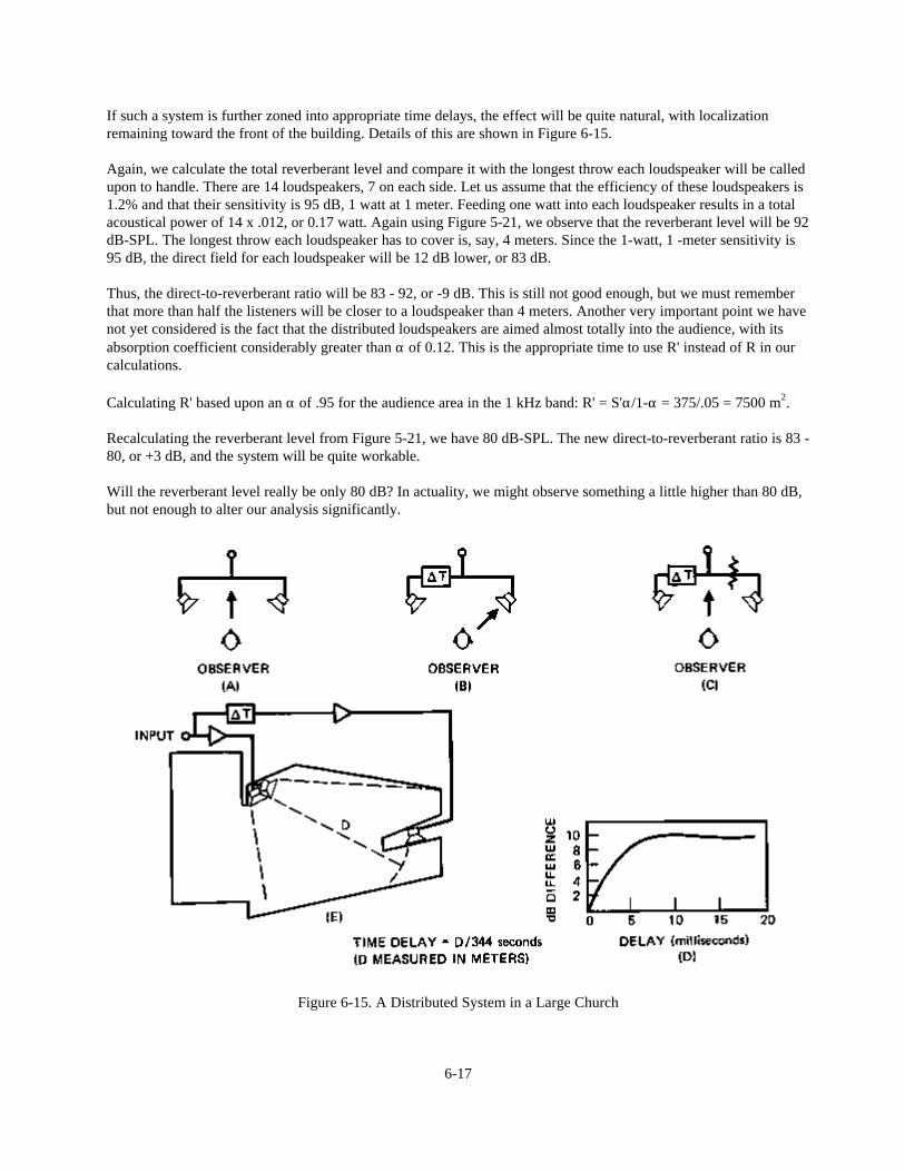
If such a system is further zoned into appropriate time delays, the effect will be quite natural, with localizationremaining toward the front of the building. Details of this are shown in Figure 6-15.

Again, we calculate the total reverberant level and compare it with the longest throw each loudspeaker will be calledupon to handle. There are 14 loudspeakers, 7 on each side. Let us assume that the efficiency of these loudspeakers is1.2% and that their sensitivity is 95 dB, 1 watt at 1 meter. Feeding one watt into each loudspeaker results in a totalacoustical power of 14 x .012, or 0.17 watt. Again using Figure 5-21, we observe that the reverberant level will be 92dB-SPL. The longest throw each loudspeaker has to cover is, say, 4 meters. Since the 1-watt, 1 -meter sensitivity is95 dB, the direct field for each loudspeaker will be 12 dB lower, or 83 dB.

Thus, the direct-to-reverberant ratio will be 83 - 92, or -9 dB. This is still not good enough, but we must rememberthat more than half the listeners will be closer to a loudspeaker than 4 meters. Another very important point we havenot yet considered is the fact that the distributed loudspeakers are aimed almost totally into the audience, with itsabsorption coefficient considerably greater than α of 0.12. This is the appropriate time to use R' instead of R in ourcalculations.

Calculating R' based upon an α of .95 for the audience area in the 1 kHz band: R' = S'α/1-α = 375/.05 = 7500 m2.

Recalculating the reverberant level from Figure 5-21, we have 80 dB-SPL. The new direct-to-reverberant ratio is 83 -80, or +3 dB, and the system will be quite workable.

Will the reverberant level really be only 80 dB? In actuality, we might observe something a little higher than 80 dB,but not enough to alter our analysis significantly.

Figure 6-15. A Distributed System in a Large Church

6-17

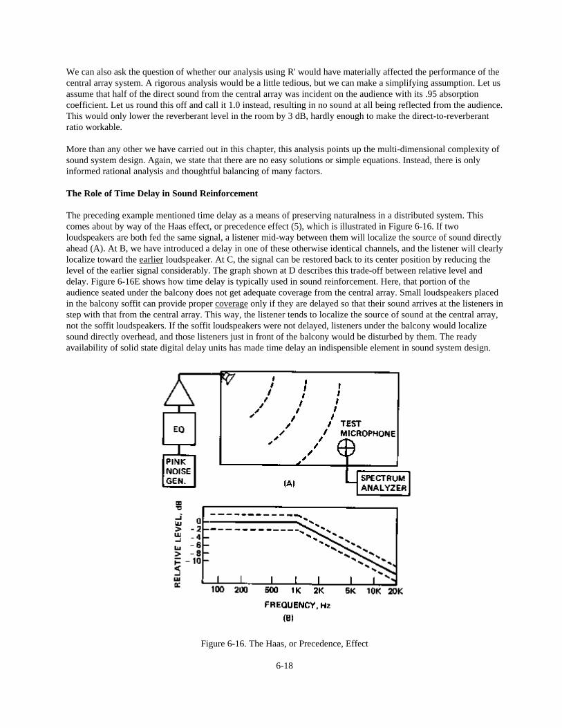
We can also ask the question of whether our analysis using R' would have materially affected the performance of thecentral array system. A rigorous analysis would be a little tedious, but we can make a simplifying assumption. Let usassume that half of the direct sound from the central array was incident on the audience with its .95 absorptioncoefficient. Let us round this off and call it 1.0 instead, resulting in no sound at all being reflected from the audience.This would only lower the reverberant level in the room by 3 dB, hardly enough to make the direct-to-reverberantratio workable.

More than any other we have carried out in this chapter, this analysis points up the multi-dimensional complexity ofsound system design. Again, we state that there are no easy solutions or simple equations. Instead, there is onlyinformed rational analysis and thoughtful balancing of many factors.

The Role of Time Delay in Sound Reinforcement

The preceding example mentioned time delay as a means of preserving naturalness in a distributed system. Thiscomes about by way of the Haas effect, or precedence effect (5), which is illustrated in Figure 6-16. If twoloudspeakers are both fed the same signal, a listener mid-way between them will localize the source of sound directlyahead (A). At B, we have introduced a delay in one of these otherwise identical channels, and the listener will clearlylocalize toward the earlier loudspeaker. At C, the signal can be restored back to its center position by reducing thelevel of the earlier signal considerably. The graph shown at D describes this trade-off between relative level anddelay. Figure 6-16E shows how time delay is typically used in sound reinforcement. Here, that portion of theaudience seated under the balcony does not get adequate coverage from the central array. Small loudspeakers placedin the balcony soffit can provide proper coverage only if they are delayed so that their sound arrives at the listeners instep with that from the central array. This way, the listener tends to localize the source of sound at the central array,not the soffit loudspeakers. If the soffit loudspeakers were not delayed, listeners under the balcony would localizesound directly overhead, and those listeners just in front of the balcony would be disturbed by them. The readyavailability of solid state digital delay units has made time delay an indispensible element in sound system design.

Figure 6-16. The Haas, or Precedence, Effect

6-18

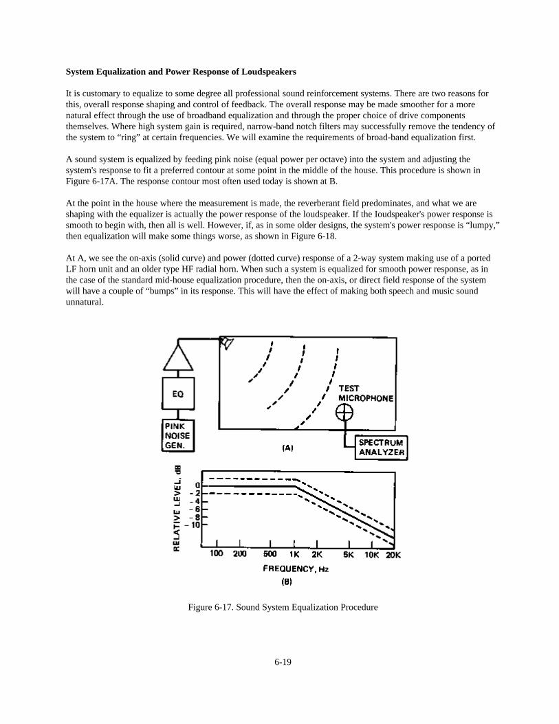
System Equalization and Power Response of Loudspeakers

It is customary to equalize to some degree all professional sound reinforcement systems. There are two reasons forthis, overall response shaping and control of feedback. The overall response may be made smoother for a morenatural effect through the use of broadband equalization and through the proper choice of drive componentsthemselves. Where high system gain is required, narrow-band notch filters may successfully remove the tendency ofthe system to “ring” at certain frequencies. We will examine the requirements of broad-band equalization first.

A sound system is equalized by feeding pink noise (equal power per octave) into the system and adjusting thesystem's response to fit a preferred contour at some point in the middle of the house. This procedure is shown inFigure 6-17A. The response contour most often used today is shown at B.

At the point in the house where the measurement is made, the reverberant field predominates, and what we areshaping with the equalizer is actually the power response of the loudspeaker. If the Ioudspeaker's power response issmooth to begin with, then all is well. However, if, as in some older designs, the system's power response is “lumpy,”then equalization will make some things worse, as shown in Figure 6-18.

At A, we see the on-axis (solid curve) and power (dotted curve) response of a 2-way system making use of a portedLF horn unit and an older type HF radial horn. When such a system is equalized for smooth power response, as inthe case of the standard mid-house equalization procedure, then the on-axis, or direct field response of the systemwill have a couple of “bumps” in its response. This will have the effect of making both speech and music soundunnatural.

Figure 6-17. Sound System Equalization Procedure

6-19

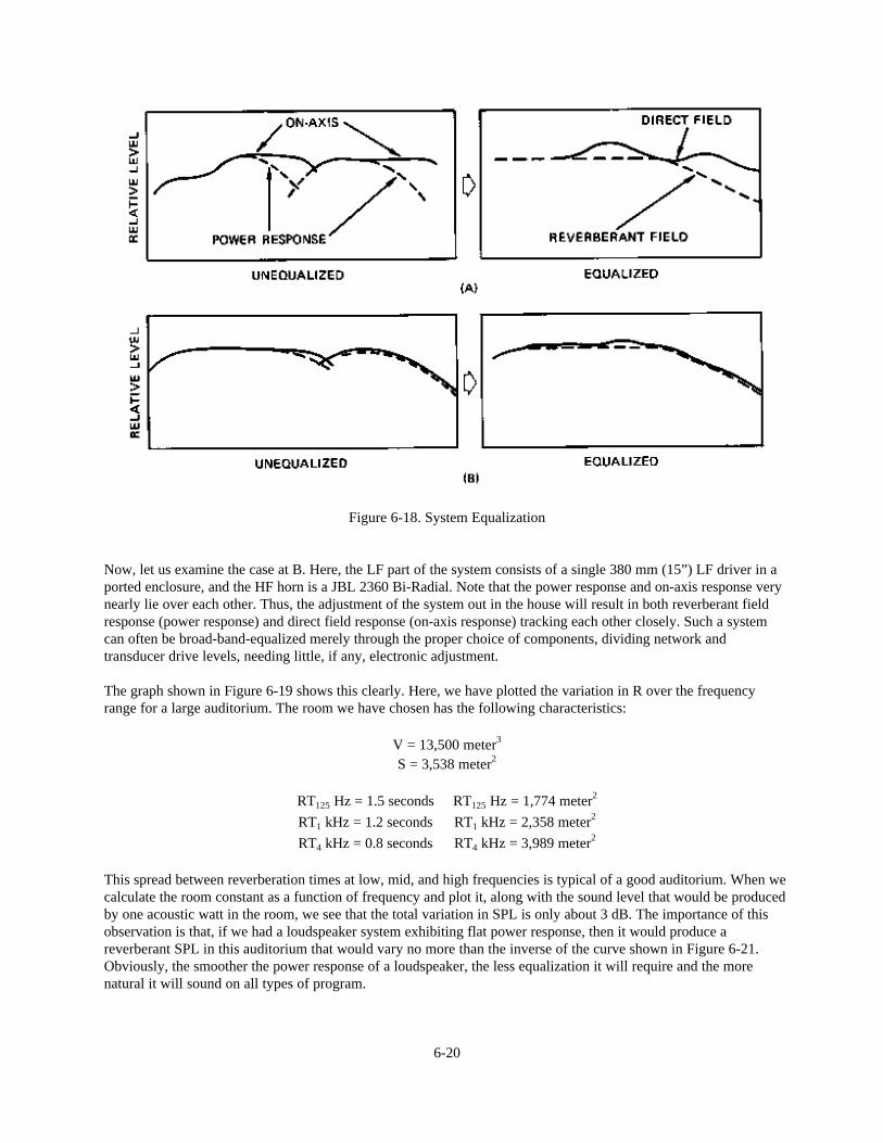
Figure 6-18. System Equalization

Now, let us examine the case at B. Here, the LF part of the system consists of a single 380 mm (15”) LF driver in aported enclosure, and the HF horn is a JBL 2360 Bi-Radial. Note that the power response and on-axis response verynearly lie over each other. Thus, the adjustment of the system out in the house will result in both reverberant fieldresponse (power response) and direct field response (on-axis response) tracking each other closely. Such a systemcan often be broad-band-equalized merely through the proper choice of components, dividing network andtransducer drive levels, needing little, if any, electronic adjustment.

The graph shown in Figure 6-19 shows this clearly. Here, we have plotted the variation in R over the frequencyrange for a large auditorium. The room we have chosen has the following characteristics:

V = 13,500 meter3

S = 3,538 meter2

RT125 Hz = 1.5 seconds RT125 Hz = 1,774 meter2

RT1 kHz = 1.2 seconds RT1 kHz = 2,358 meter2

RT4 kHz = 0.8 seconds RT4 kHz = 3,989 meter2

This spread between reverberation times at low, mid, and high frequencies is typical of a good auditorium. When wecalculate the room constant as a function of frequency and plot it, along with the sound level that would be producedby one acoustic watt in the room, we see that the total variation in SPL is only about 3 dB. The importance of thisobservation is that, if we had a loudspeaker system exhibiting flat power response, then it would produce areverberant SPL in this auditorium that would vary no more than the inverse of the curve shown in Figure 6-21.Obviously, the smoother the power response of a loudspeaker, the less equalization it will require and the morenatural it will sound on all types of program.

6-20

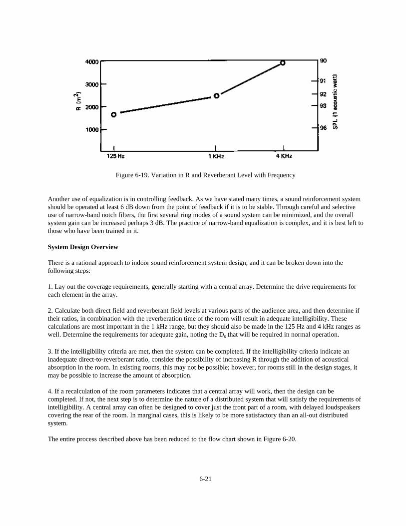
Figure 6-19. Variation in R and Reverberant Level with Frequency

Another use of equalization is in controlling feedback. As we have stated many times, a sound reinforcement systemshould be operated at least 6 dB down from the point of feedback if it is to be stable. Through careful and selectiveuse of narrow-band notch filters, the first several ring modes of a sound system can be minimized, and the overallsystem gain can be increased perhaps 3 dB. The practice of narrow-band equalization is complex, and it is best left tothose who have been trained in it.

System Design Overview

There is a rational approach to indoor sound reinforcement system design, and it can be broken down into thefollowing steps:

1. Lay out the coverage requirements, generally starting with a central array. Determine the drive requirements foreach element in the array.

2. Calculate both direct field and reverberant field levels at various parts of the audience area, and then determine iftheir ratios, in combination with the reverberation time of the room will result in adequate intelligibility. Thesecalculations are most important in the 1 kHz range, but they should also be made in the 125 Hz and 4 kHz ranges aswell. Determine the requirements for adequate gain, noting the Ds that will be required in normal operation.

3. If the intelligibility criteria are met, then the system can be completed. If the intelligibility criteria indicate aninadequate direct-to-reverberant ratio, consider the possibility of increasing R through the addition of acousticalabsorption in the room. In existing rooms, this may not be possible; however, for rooms still in the design stages, itmay be possible to increase the amount of absorption.

4. If a recalculation of the room parameters indicates that a central array will work, then the design can becompleted. If not, the next step is to determine the nature of a distributed system that will satisfy the requirements ofintelligibility. A central array can often be designed to cover just the front part of a room, with delayed loudspeakerscovering the rear of the room. In marginal cases, this is likely to be more satisfactory than an all-out distributedsystem.

The entire process described above has been reduced to the flow chart shown in Figure 6-20.

6-21

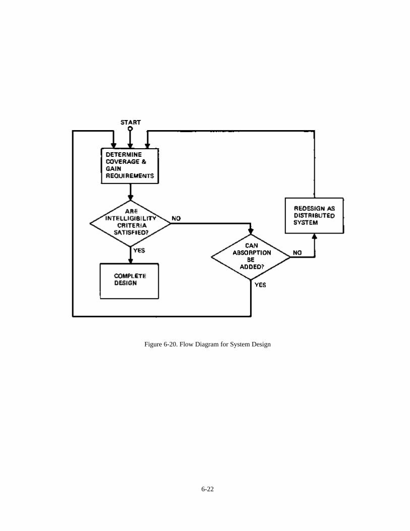
Figure 6-20. Flow Diagram for System Design

6-22

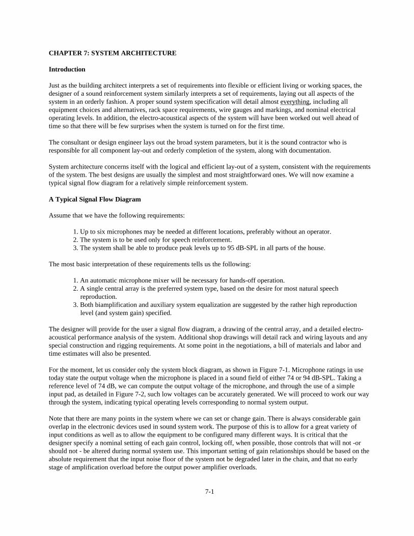
CHAPTER 7: SYSTEM ARCHITECTURE

Introduction

Just as the building architect interprets a set of requirements into flexible or efficient living or working spaces, thedesigner of a sound reinforcement system similarly interprets a set of requirements, laying out all aspects of thesystem in an orderly fashion. A proper sound system specification will detail almost everything, including allequipment choices and alternatives, rack space requirements, wire gauges and markings, and nominal electricaloperating levels. In addition, the electro-acoustical aspects of the system will have been worked out well ahead oftime so that there will be few surprises when the system is turned on for the first time.

The consultant or design engineer lays out the broad system parameters, but it is the sound contractor who isresponsible for all component lay-out and orderly completion of the system, along with documentation.

System architecture concerns itself with the logical and efficient lay-out of a system, consistent with the requirementsof the system. The best designs are usually the simplest and most straightforward ones. We will now examine atypical signal flow diagram for a relatively simple reinforcement system.

A Typical Signal Flow Diagram

Assume that we have the following requirements:

1. Up to six microphones may be needed at different locations, preferably without an operator.2. The system is to be used only for speech reinforcement.3. The system shall be able to produce peak levels up to 95 dB-SPL in all parts of the house.

The most basic interpretation of these requirements tells us the following:

1. An automatic microphone mixer will be necessary for hands-off operation.2. A single central array is the preferred system type, based on the desire for most natural speech reproduction.3. Both biamplification and auxiliary system equalization are suggested by the rather high reproduction level (and system gain) specified.

The designer will provide for the user a signal flow diagram, a drawing of the central array, and a detailed electro-acoustical performance analysis of the system. Additional shop drawings will detail rack and wiring layouts and anyspecial construction and rigging requirements. At some point in the negotiations, a bill of materials and labor andtime estimates will also be presented.

For the moment, let us consider only the system block diagram, as shown in Figure 7-1. Microphone ratings in usetoday state the output voltage when the microphone is placed in a sound field of either 74 or 94 dB-SPL. Taking areference level of 74 dB, we can compute the output voltage of the microphone, and through the use of a simpleinput pad, as detailed in Figure 7-2, such low voltages can be accurately generated. We will proceed to work our waythrough the system, indicating typical operating levels corresponding to normal system output.

Note that there are many points in the system where we can set or change gain. There is always considerable gainoverlap in the electronic devices used in sound system work. The purpose of this is to allow for a great variety ofinput conditions as well as to allow the equipment to be configured many different ways. It is critical that thedesigner specify a nominal setting of each gain control, locking off, when possible, those controls that will not -orshould not - be altered during normal system use. This important setting of gain relationships should be based on theabsolute requirement that the input noise floor of the system not be degraded later in the chain, and that no earlystage of amplification overload before the output power amplifier overloads.

7-1

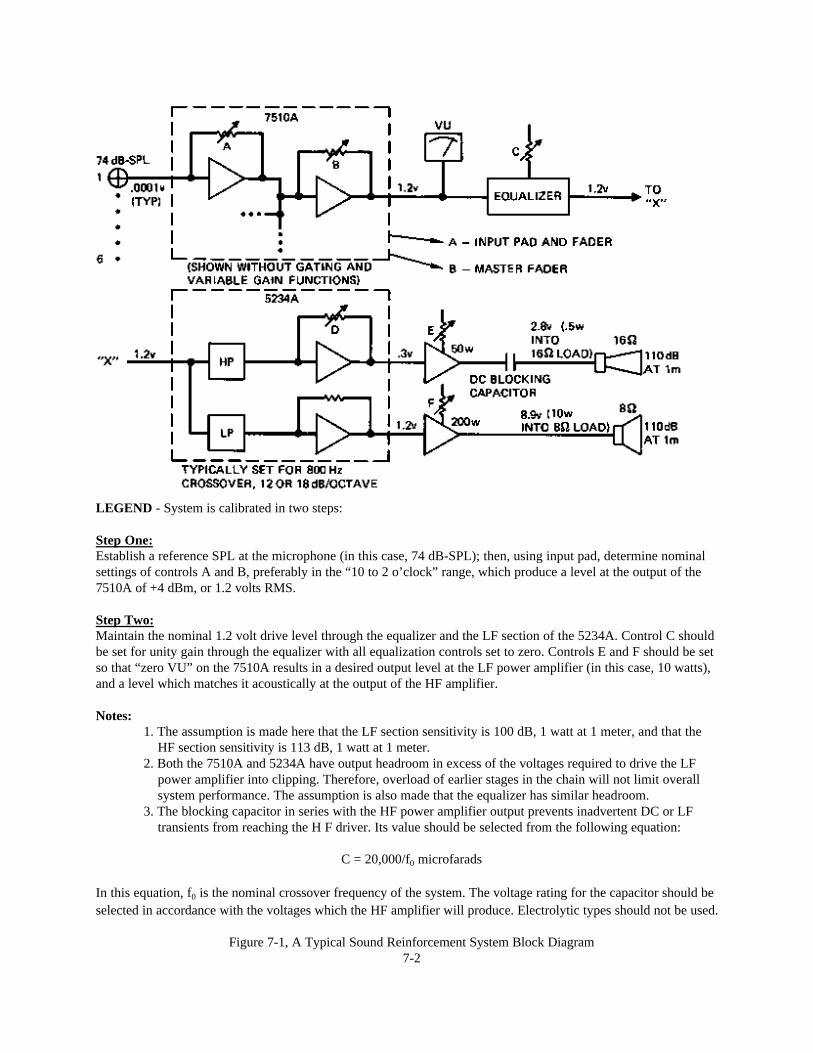
LEGEND - System is calibrated in two steps:

Step One:Establish a reference SPL at the microphone (in this case, 74 dB-SPL); then, using input pad, determine nominalsettings of controls A and B, preferably in the “10 to 2 o’clock” range, which produce a level at the output of the7510A of +4 dBm, or 1.2 volts RMS.

Step Two:Maintain the nominal 1.2 volt drive level through the equalizer and the LF section of the 5234A. Control C shouldbe set for unity gain through the equalizer with all equalization controls set to zero. Controls E and F should be setso that “zero VU” on the 7510A results in a desired output level at the LF power amplifier (in this case, 10 watts),and a level which matches it acoustically at the output of the HF amplifier.

Notes:1. The assumption is made here that the LF section sensitivity is 100 dB, 1 watt at 1 meter, and that the HF section sensitivity is 113 dB, 1 watt at 1 meter.2. Both the 7510A and 5234A have output headroom in excess of the voltages required to drive the LF power amplifier into clipping. Therefore, overload of earlier stages in the chain will not limit overall system performance. The assumption is also made that the equalizer has similar headroom.3. The blocking capacitor in series with the HF power amplifier output prevents inadvertent DC or LF transients from reaching the H F driver. Its value should be selected from the following equation:

C = 20,000/f0 microfarads

In this equation, f0 is the nominal crossover frequency of the system. The voltage rating for the capacitor should beselected in accordance with the voltages which the HF amplifier will produce. Electrolytic types should not be used.

Figure 7-1, A Typical Sound Reinforcement System Block Diagram7-2

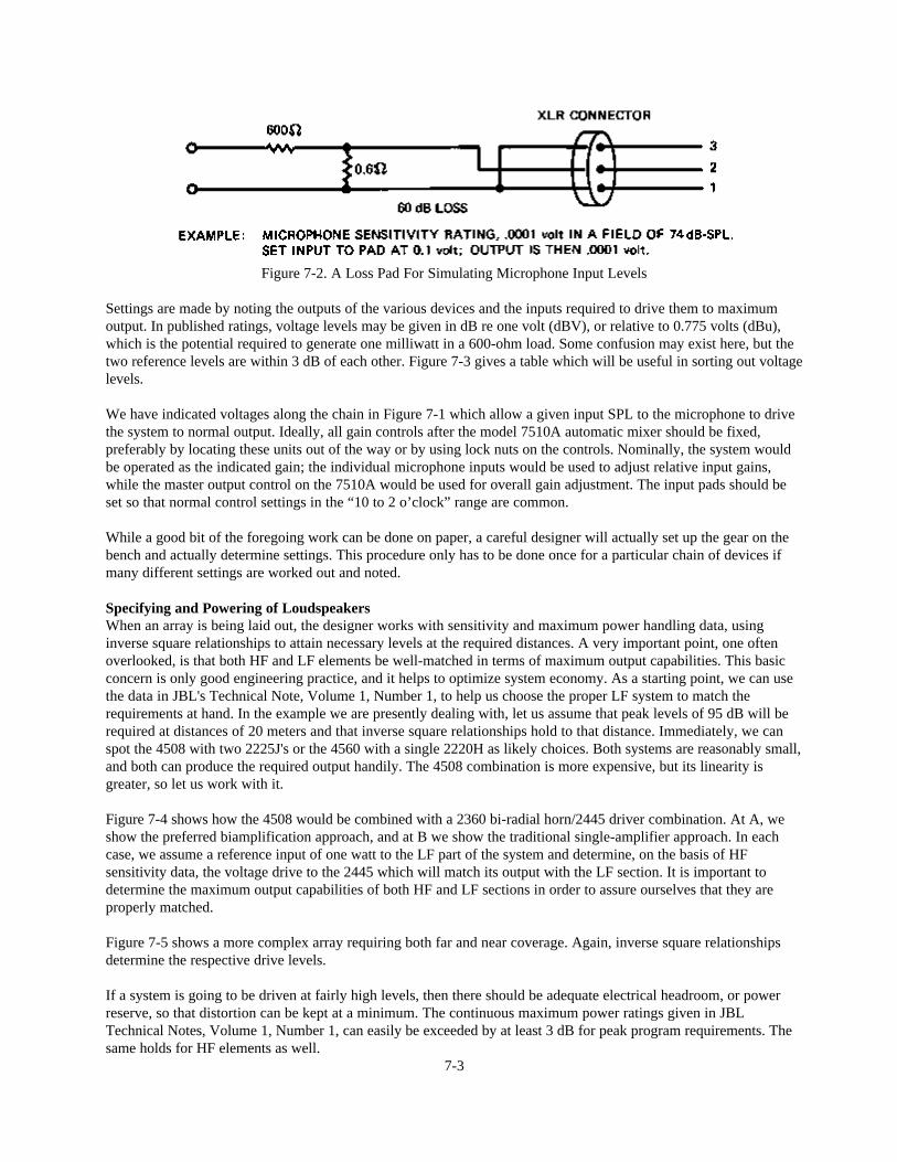
Figure 7-2. A Loss Pad For Simulating Microphone Input Levels

Settings are made by noting the outputs of the various devices and the inputs required to drive them to maximumoutput. In published ratings, voltage levels may be given in dB re one volt (dBV), or relative to 0.775 volts (dBu),which is the potential required to generate one milliwatt in a 600-ohm load. Some confusion may exist here, but thetwo reference levels are within 3 dB of each other. Figure 7-3 gives a table which will be useful in sorting out voltagelevels.

We have indicated voltages along the chain in Figure 7-1 which allow a given input SPL to the microphone to drivethe system to normal output. Ideally, all gain controls after the model 7510A automatic mixer should be fixed,preferably by locating these units out of the way or by using lock nuts on the controls. Nominally, the system wouldbe operated as the indicated gain; the individual microphone inputs would be used to adjust relative input gains,while the master output control on the 7510A would be used for overall gain adjustment. The input pads should beset so that normal control settings in the “10 to 2 o’clock” range are common.

While a good bit of the foregoing work can be done on paper, a careful designer will actually set up the gear on thebench and actually determine settings. This procedure only has to be done once for a particular chain of devices ifmany different settings are worked out and noted.

Specifying and Powering of LoudspeakersWhen an array is being laid out, the designer works with sensitivity and maximum power handling data, usinginverse square relationships to attain necessary levels at the required distances. A very important point, one oftenoverlooked, is that both HF and LF elements be well-matched in terms of maximum output capabilities. This basicconcern is only good engineering practice, and it helps to optimize system economy. As a starting point, we can usethe data in JBL's Technical Note, Volume 1, Number 1, to help us choose the proper LF system to match therequirements at hand. In the example we are presently dealing with, let us assume that peak levels of 95 dB will berequired at distances of 20 meters and that inverse square relationships hold to that distance. Immediately, we canspot the 4508 with two 2225J's or the 4560 with a single 2220H as likely choices. Both systems are reasonably small,and both can produce the required output handily. The 4508 combination is more expensive, but its linearity isgreater, so let us work with it.

Figure 7-4 shows how the 4508 would be combined with a 2360 bi-radial horn/2445 driver combination. At A, weshow the preferred biamplification approach, and at B we show the traditional single-amplifier approach. In eachcase, we assume a reference input of one watt to the LF part of the system and determine, on the basis of HFsensitivity data, the voltage drive to the 2445 which will match its output with the LF section. It is important todetermine the maximum output capabilities of both HF and LF sections in order to assure ourselves that they areproperly matched.

Figure 7-5 shows a more complex array requiring both far and near coverage. Again, inverse square relationshipsdetermine the respective drive levels.

If a system is going to be driven at fairly high levels, then there should be adequate electrical headroom, or powerreserve, so that distortion can be kept at a minimum. The continuous maximum power ratings given in JBLTechnical Notes, Volume 1, Number 1, can easily be exceeded by at least 3 dB for peak program requirements. Thesame holds for HF elements as well.

7-3

Figure 7-3, dBV and dBu

Figure 7-4. Matching HF and LF Components

7-4

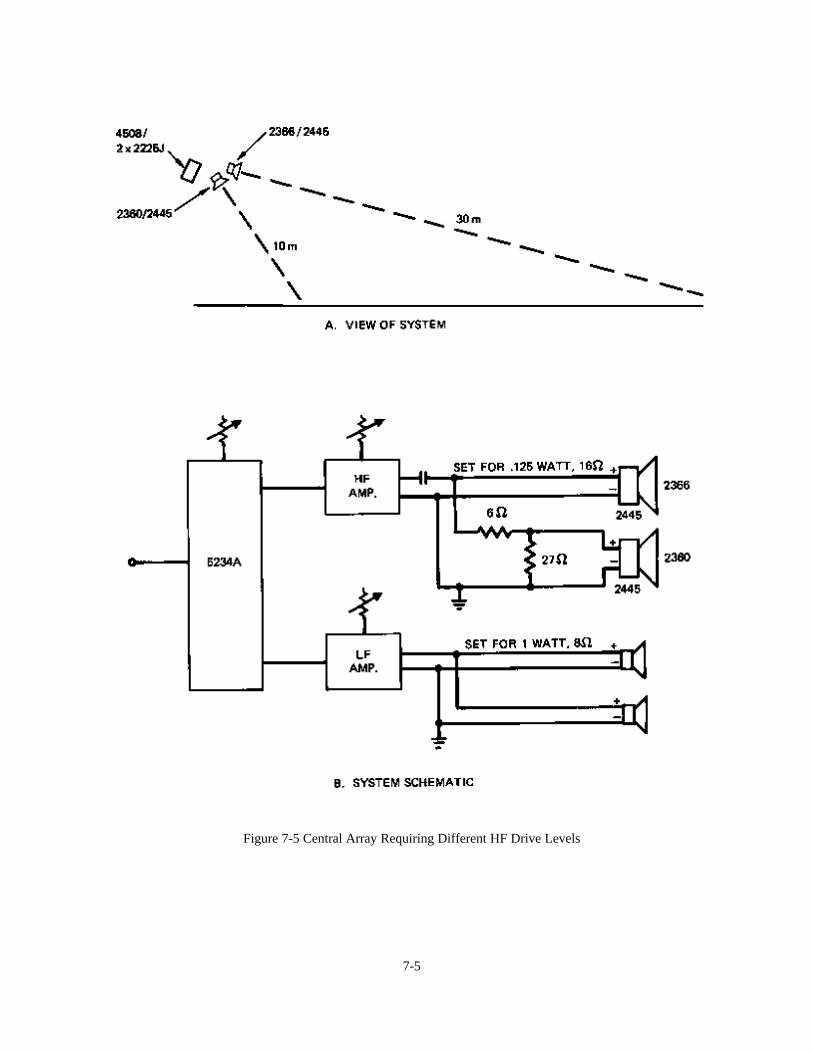
Figure 7-5 Central Array Requiring Different HF Drive Levels

7-5

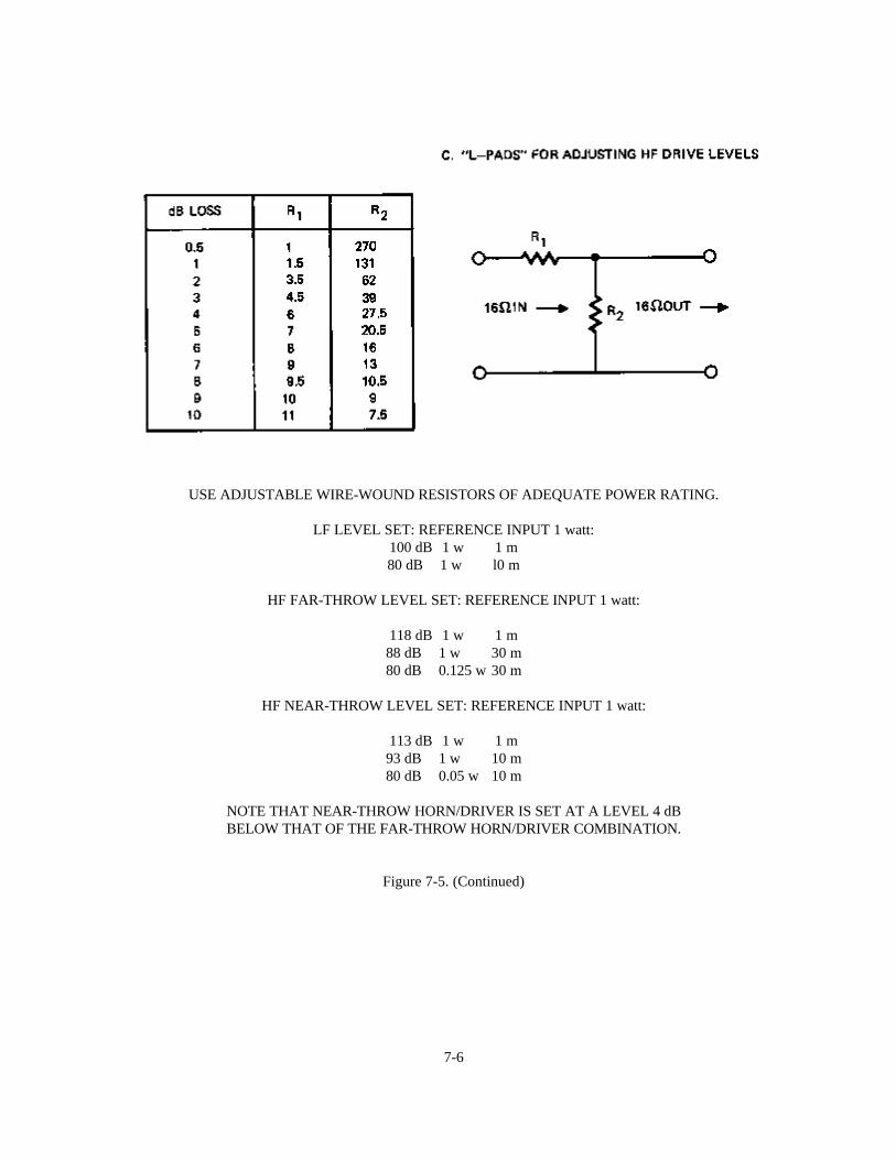
USE ADJUSTABLE WIRE-WOUND RESISTORS OF ADEQUATE POWER RATING.

LF LEVEL SET: REFERENCE INPUT 1 watt:100 dB 1 w 1 m80 dB 1 w l0 m

HF FAR-THROW LEVEL SET: REFERENCE INPUT 1 watt:

118 dB 1 w 1 m88 dB 1 w 30 m80 dB 0.125 w 30 m

HF NEAR-THROW LEVEL SET: REFERENCE INPUT 1 watt:

113 dB 1 w 1 m93 dB 1 w 10 m80 dB 0.05 w 10 m

NOTE THAT NEAR-THROW HORN/DRIVER IS SET AT A LEVEL 4 dBBELOW THAT OF THE FAR-THROW HORN/DRIVER COMBINATION.

Figure 7-5. (Continued)

7-6

In laying out and powering a system, we recommend that the design requirements be based on the conservativecontinuous output capabilities of the devices, allowing a 3-dB, or twice-power, safety margin over the averagecontinuous rating. Thus, a 4508 with a pair of 2225J's should be powered with 800 watts, ideally, for 3 dB headroomover the system's continuous rating of 400 watts.

The poling, or phasing, of HF and LF components is a very important consideration. In general, JBL's instructionsincluded with passive networks should be carefully followed. Where the 5234A is used, the poling of components isentirely in the hands of the contractor or designer. The important considerations are that there be no cancellationbetween the two components at the crossover frequency and that the voice coils lie, if possible, in the same plane - orbe displaced from each other an integral number of wavelengths at the crossover frequency. The 12 dB/octavenetworks require that one of the components be connected electrically out-of-phase for proper response. With the 18dB/octave networks, 1(he connection may be made either way. Please follow instructions where they are given, andby all means be consistent!

In the following sections of this chapter, we will present a number of case studies. For each of these, we will assumethat all calculations of gain and intelligibility requirements have been made and that the system satisfy thoserequirements. Our emphasis here will be primarily on the hardware implementation of the systems.

A - Multi-channel Reinforcement System in a Theater

Many of these systems are five-channel, in order to preserve a continuum of sound across the proscenium. Here, wewill consider only a three-channel system. Additional requirements of the system are:

1. Delayed feed to under-balcony areas2. Extra channels for on-stage monitoring (fold-back)3. Input facilities for sound effects

A typical theater will have a short reverberation time, and critical distance may be fairly large, due to the high valueof R. For realistic performance, high levels may be called for. Let us assume that the three arrays over theproscenium may be called upon to produce levels at 25 meters of 105 dB-SPL. As usual, the place to start is with LFrequirements. Referring to Technical Note Volume 1, Number 1, we see that a single 4508 with 2x2225J's willproduce a maximum continuous level of 96 dB at 30 meters. By inverse square law, this is equivalent of 97 dB at adistance of 25 meters. Figure 7-6 shows the effect of combining HF and LF elements. Crossing over at 800 Hz resultsin the entire audio band being almost equally divided between the LF and HF elements. Since the 2360/2445combination has adequate output reserve, it can be level-matched with the 4508/2225J combination at full output,and the combination of the two sections will result in a 3-dB level increase over either one alone.

Now we can consider the effect of adding all three channels together. For random program input, the averagesummation of the three will produce a level increase of 10 log (3), or about 5 dB. This puts us at 105 dB, our designgoal.

The heart of such a system as we are discussing here is the console. There are many stock units available today withfeatures tailored to theatrical use. Such units are far cheaper in cost that custom-designed units and should be usedwhen possible. Figure 7-7 shows the overall system lay-out. Biamplification is a necessity in such a system as this,and it is best if shielded leads can be run all the way up to the proscenium so that power amplifiers can be locatedadjacent to the loudspeaker systems. The alternative to this is to make long runs of very heavy gauge wire. Figure 7-8shows the resistance characteristics of various wire gauges as a function of distance. The goal in any long run shouldbe to keep the power loss 0.5 dB or less. Let us assume that there is a distance of 80 meters between the amplifierand the loudspeakers. The simple calculations show that AWG #10 copper wire, or larger, must be used in order tokeep losses at the .5 dB point. Distribution transformers, even of high quality and power rating, should not be usedin systems of this type to hold down line losses. As we have stated, the only sensible solution is to power theloudspeakers at the proscenium.

7-7

Figure 7-6. Acoustical Summation of HF and LF Sections

Figure 7-7. A Three-Channel Theater Reinforcement System

7-8

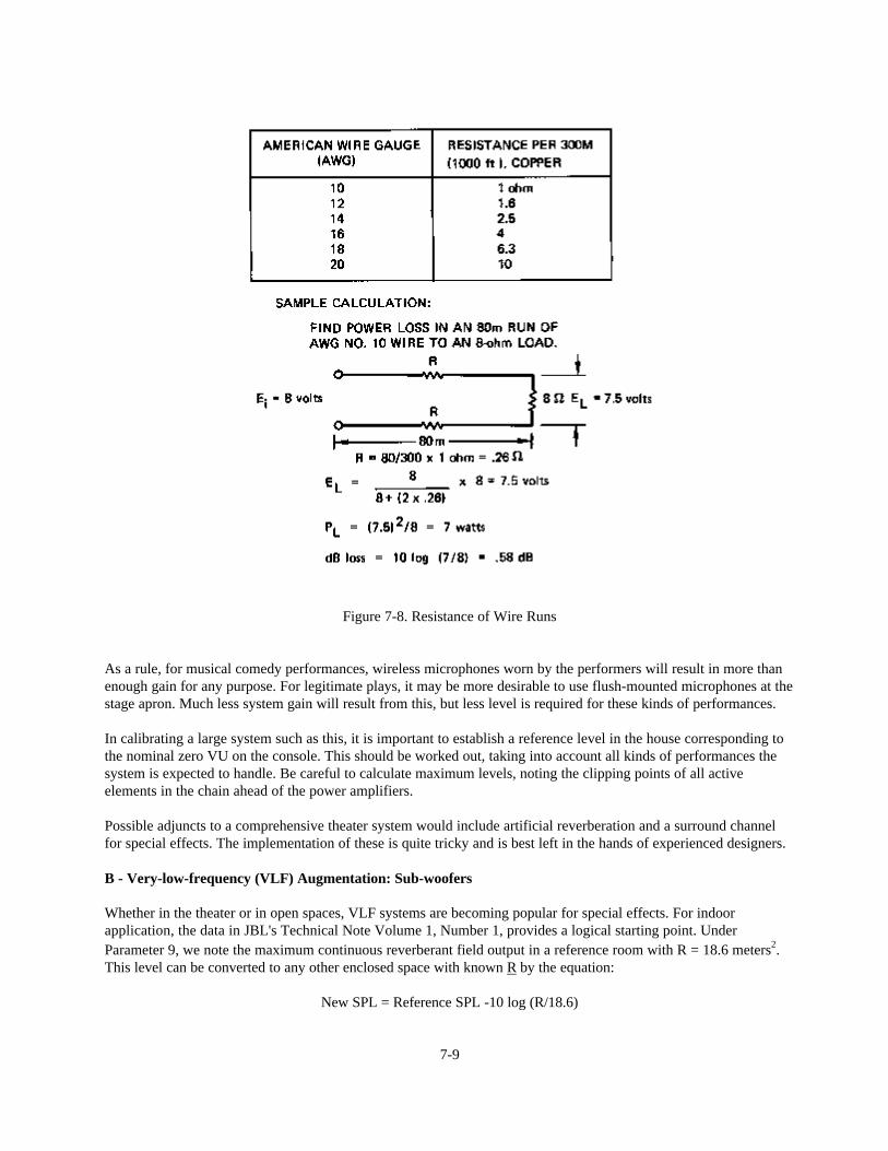
Figure 7-8. Resistance of Wire Runs

As a rule, for musical comedy performances, wireless microphones worn by the performers will result in more thanenough gain for any purpose. For legitimate plays, it may be more desirable to use flush-mounted microphones at thestage apron. Much less system gain will result from this, but less level is required for these kinds of performances.

In calibrating a large system such as this, it is important to establish a reference level in the house corresponding tothe nominal zero VU on the console. This should be worked out, taking into account all kinds of performances thesystem is expected to handle. Be careful to calculate maximum levels, noting the clipping points of all activeelements in the chain ahead of the power amplifiers.

Possible adjuncts to a comprehensive theater system would include artificial reverberation and a surround channelfor special effects. The implementation of these is quite tricky and is best left in the hands of experienced designers.

B - Very-low-frequency (VLF) Augmentation: Sub-woofers

Whether in the theater or in open spaces, VLF systems are becoming popular for special effects. For indoorapplication, the data in JBL's Technical Note Volume 1, Number 1, provides a logical starting point. UnderParameter 9, we note the maximum continuous reverberant field output in a reference room with R = 18.6 meters2.This level can be converted to any other enclosed space with known R by the equation:

New SPL = Reference SPL -10 log (R/18.6)

7-9

Since we are dealing with sound in the 20-25 Hz range up to 40-50 Hz, we have to make some simplifyingassumptions, since there is little measured data on enclosed spaces in the VLF range. Generally, it is safe to assumethat the room constant in the 25-50 Hz range is roughly the same as in the 125 Hz range. Exceptions here may berooms whose boundaries are fairly thin and flimsy. Even then, measured data may not differ from calculated data bymore than 2 or 3 dB.

Mutual coupling is an important factor in the summation of VLF systems. Figure 7-9A shows the transmissioncoefficient for a direct radiator as a function of cone diameters. The solid curve is for a single unit, and the dottedcurve is for two units operating together. In addition to the doubled power handling capability afforded by the twounits, the dotted curve shows a 3-dB increase in transmission coefficient at low frequencies. This is due basically tothe tendency of the two loudspeakers to behave as a single unit with larger cone diameter, and hence higherefficiency. Thus, at B, we see the relative responses of a single woofer (solid curve) compared to two such radiators(dashed curve). Note that the upper frequency transition point for the pair is 0.7 that of the single unit. The moresuch units we combine, the lower the effective cut-off frequency drops.

As an example, let us pick a large theater with the following physical parameters:

V = 14,000 meter3

S= 3700 meter2

T60 = 1.2 secondsR= 2500 meter2

Figure 7-9. Mutual Coupling

7-10

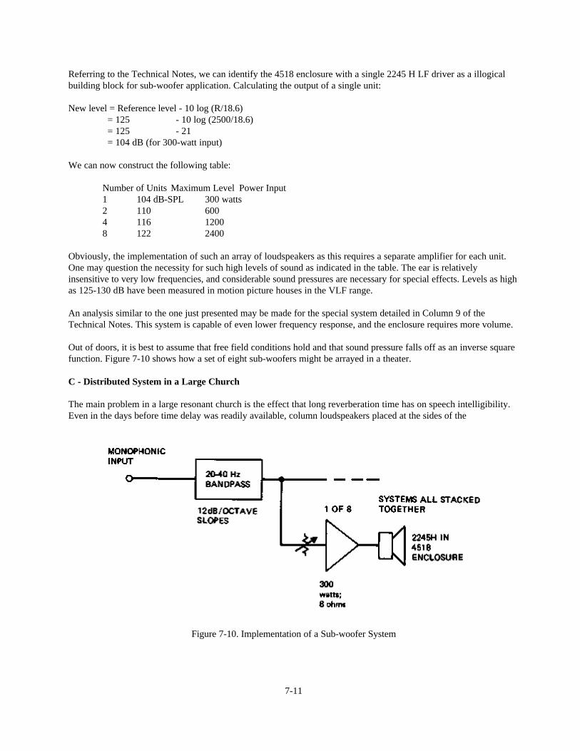
Referring to the Technical Notes, we can identify the 4518 enclosure with a single 2245 H LF driver as a illogicalbuilding block for sub-woofer application. Calculating the output of a single unit:

New level = Reference level - 10 log (R/18.6) = 125 - 10 log (2500/18.6) = 125 - 21 = 104 dB (for 300-watt input)

We can now construct the following table:

Number of Units Maximum Level Power Input1 104 dB-SPL 300 watts2 110 6004 116 12008 122 2400

Obviously, the implementation of such an array of loudspeakers as this requires a separate amplifier for each unit.One may question the necessity for such high levels of sound as indicated in the table. The ear is relativelyinsensitive to very low frequencies, and considerable sound pressures are necessary for special effects. Levels as highas 125-130 dB have been measured in motion picture houses in the VLF range.

An analysis similar to the one just presented may be made for the special system detailed in Column 9 of theTechnical Notes. This system is capable of even lower frequency response, and the enclosure requires more volume.

Out of doors, it is best to assume that free field conditions hold and that sound pressure falls off as an inverse squarefunction. Figure 7-10 shows how a set of eight sub-woofers might be arrayed in a theater.

C - Distributed System in a Large Church

The main problem in a large resonant church is the effect that long reverberation time has on speech intelligibility.Even in the days before time delay was readily available, column loudspeakers placed at the sides of the

Figure 7-10. Implementation of a Sub-woofer System

7-11

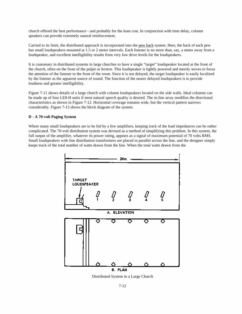
church offered the best performance - and probably for the least cost. In conjunction with time delay, columnspeakers can provide extremely natural reinforcement.

Carried to its limit, the distributed approach is incorporated into the pew back system. Here, the back of each pewhas small loudspeakers mounted at 1.5 or 2 meter intervals. Each listener is no more than, say, a meter away from aloudspeaker, and excellent intelligibility results from very low drive levels for the loudspeakers.

It is customary in distributed systems in large churches to have a single “target” loudspeaker located at the front ofthe church, often on the front of the pulpit or lectern. This loudspeaker is lightly powered and merely serves to focusthe attention of the listener to the front of the room. Since it is not delayed, the target loudspeaker is easily localizedby the listener as the apparent source of sound. The function of the nearer delayed loudspeakers is to provideloudness and greater intelligibility.

Figure 7-11 shows details of a large church with column loudspeakers located on the side walls. Ideal columns canbe made up of four LE8-H units if most natural speech quality is desired. The in-line array modifies the directionalcharacteristics as shown in Figure 7-12. Horizontal coverage remains wide, but the vertical pattern narrowsconsiderably. Figure 7-13 shows the block diagram of the system.

D - A 70-volt Paging System

Where many small loudspeakers are to be fed by a few amplifiers, keeping track of the load impedances can be rathercomplicated. The 70-volt distribution system was devised as a method of simplifying this problem. In this system, thefull output of the amplifier, whatever its power rating, appears as a signal of maximum potential of 70 volts RMS.Small loudspeakers with line distribution transformers are placed in parallel across the line, and the designer simplykeeps track of the total number of watts drawn from the line. When the total watts drawn from the

Distributed System in a Large Church

7-12

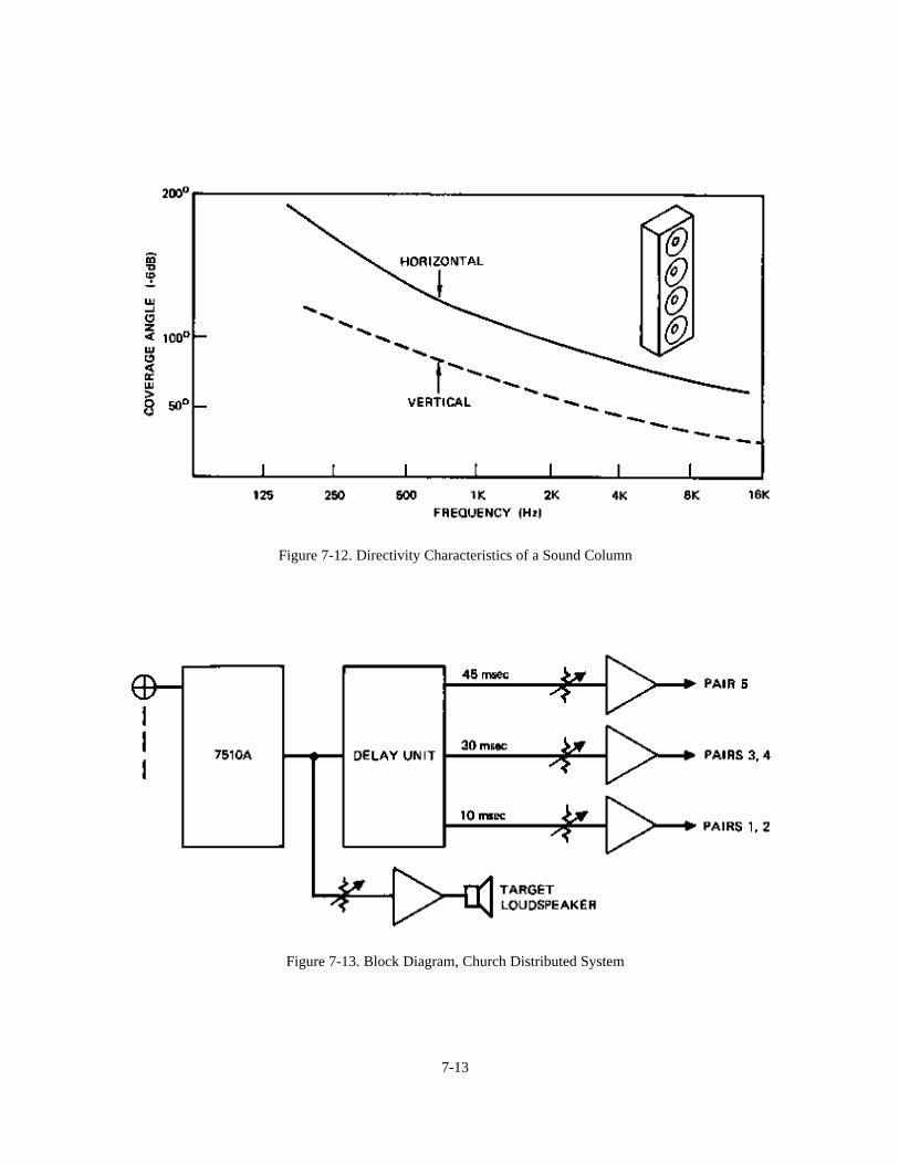
Figure 7-12. Directivity Characteristics of a Sound Column

Figure 7-13. Block Diagram, Church Distributed System

7-13

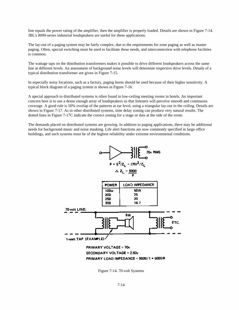
line equals the power rating of the amplifier, then the amplifier is properly loaded. Details are shown in Figure 7-14.JBL's 8000-series industrial loudspeakers are useful for these applications.

The lay-out of a paging system may be fairly complex, due to the requirements for zone paging as well as masterpaging. Often, special switching must be used to facilitate these needs, and interconnection with telephone facilitiesis common.

The wattage taps on the distribution transformers makes it possible to drive different loudspeakers across the sameline at different levels. An assessment of background noise levels will determine respective drive levels. Details of atypical distribution transformer are given in Figure 7-15.

In especially noisy locations, such as a factory, paging horns should be used because of their higher sensitivity. Atypical block diagram of a paging system is shown in Figure 7-16.

A special approach to distributed systems is often found in low-ceiling meeting rooms in hotels. An importantconcern here is to use a dense enough array of loudspeakers so that listeners will perceive smooth and continuouscoverage. A good rule is 50% overlap of the patterns at ear level, using a triangular lay-out in the ceiling. Details areshown in Figure 7-17. As in other distributed systems, time delay zoning can produce very natural results. Thedotted lines in Figure 7-17C indicate the correct zoning for a stage or dais at the side of the room.

The demands placed on distributed systems are growing. In addition to paging applications, there may be additionalneeds for background music and noise masking. Life alert functions are now commonly specified in large officebuildings, and such systems must be of the highest reliability under extreme environmental conditions.

Figure 7-14. 70-volt Systems

7-14

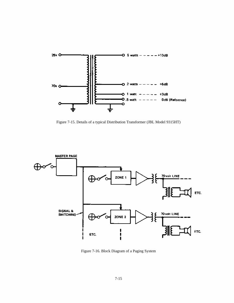
Figure 7-15. Details of a typical Distribution Transformer (JBL Model 9315HT)

Figure 7-16. Block Diagram of a Paging System

7-15

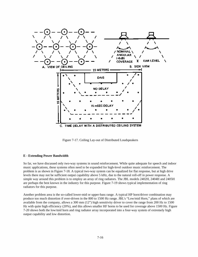
Figure 7-17. Ceiling Lay-out of Distributed Loudspeakers

E - Extending Power Bandwidth

So far, we have discussed only two-way systems in sound reinforcement. While quite adequate for speech and indoormusic applications, these systems often need to be expanded for high-level outdoor music reinforcement. Theproblem is as shown in Figure 7-18. A typical two-way system can be equalized for flat response, but at high drivelevels there may not be sufficient output capability above 5 kHz, due to the natural roll-off in power response. Asimple way around this problem is to employ an array of ring radiators. The JBL models 2402H, 2404H and 2405Hare perhaps the best known in the industry for this purpose. Figure 7-19 shows typical implementation of ringradiators for this purpose.

Another problem area is the so-called lower-mid or upper-bass range. A typical HP horn/driver combination mayproduce too much distortion if over-driven in the 800 to 1500 Hz range. JBL's “Low/mid Horn,” plans of which areavailable from the company, allows a 300 mm (12”) high sensitivity driver to cover the range from 200 Hz to 1500Hz with quite high efficiency (20%), and this allows smaller HF horns to be used for coverage above 1500 Hz. Figure7-20 shows both the low/mid horn and ring radiator array incorporated into a four-way system of extremely highoutput capability and low distortion.

7-16

Figure 7-18, Power Bandwidth Limitations

Figure 7-19. HF Augmentation with Ring Radiators

7-17

Figure 7-20. A Four-way System of High Output Capability

7-18

RECOMMENDED READING

Books and Anthologies:

1. D. and C. Davis, Sound System Engineering 2nd ed. (Howard F. Sams, Indianapolis, 1987)

2. J. Eargle, The Microphone Handbook. (Elar, Planview, New York, 1982)

3. Various, Sound Reinforcement. (an anthology of articles on sound reinforcement from the pages of the J. Audio Eng. Soc., vol. 1 through vol. 26).

Papers:

4. C. P. and R. E. Boner, “The Gain of a Sound System,” J. Audio Eng. Soc., vol. 17, no. 2 (1969).

5. H. Haas, “The Influence of a Single Echo on the Audibility of Speech,” J. Audio Eng. Soc., vol. 20 no. 2 (1972)

6. H.F. Hopkins and N. R. Stryker, “A Proposed Loudness-Efficiency Rating for Loudspeakers and the Determination of System Power Requirements for Enclosures,” Proceedings of the I. R. E., March 1948.

7. C.T. Molloy, “Calculation of the Directivity Index for Various Types of Radiators,” J. Acoust. Soc. Amer., vol. 20, p. 387-405 (1948).

8. V.M. A Peutz, “Articulation Loss of Consonants as a Criterion for Speech Transmission in a Room,” J. Audio Eng. Soc., vol. 19, no. 11 (1971).

9. V. M. A. Peutz, “Quasi-steady-state and Decaying Sound Fields,” Ingenieursblad, vol. 42, no. 18 (1973) (in Dutch)