Embed Size (px)
Citation preview

Louisiana State University Louisiana State University
LSU Digital Commons LSU Digital Commons
LSU Doctoral Dissertations Graduate School
5-14-2020
Source Apportionment of Ozone and Its Health Effects in North Source Apportionment of Ozone and Its Health Effects in North
China Plain and Southeast U.S. China Plain and Southeast U.S.
Kaiyu Chen Louisiana State University and Agricultural and Mechanical College
Follow this and additional works at: https://digitalcommons.lsu.edu/gradschool_dissertations
Part of the Environmental Engineering Commons
Recommended Citation Recommended Citation Chen, Kaiyu, "Source Apportionment of Ozone and Its Health Effects in North China Plain and Southeast U.S." (2020). LSU Doctoral Dissertations. 5254. https://digitalcommons.lsu.edu/gradschool_dissertations/5254
This Dissertation is brought to you for free and open access by the Graduate School at LSU Digital Commons. It has been accepted for inclusion in LSU Doctoral Dissertations by an authorized graduate school editor of LSU Digital Commons. For more information, please [email protected].

SOURCE APPORTIONMENT OF OZONE AND ITS HEALTH EFFECTS IN
NORTH CHINA PLAIN AND SOUTHEAST U.S.
A Dissertation
Submitted to the Graduate Faculty of the
Louisiana State University and
Agricultural and Mechanical College
in partial fulfillment of the
requirements for the degree of
Doctor of Philosophy
in
The Department of Civil and Environmental Engineering
by
Kaiyu Chen
B.S., China University of Mining and Technology, Beijing, 2014
M.S., China University of Mining and Technology, Beijing, 2017
May 2020

ii
ACKNOWLEDGEMENTS
I would like to thank my advisors, Dr. Hongliang Zhang and Xiuping Zhu, for their
supports on the projects and guiding me on my academic career. This dissertation would not
have been accomplished without their help.
Then, I want to show appreciation to my committee members (in the alphabetic order),
Dr. Eurico J D’Sa, Dr. Nina Lam and Dr. John Pardue for providing valuable suggestions on this
dissertation.
I also want to express my gratitude to all the instructors I have had courses with. Thanks
to my colleagues, my friends, our department and LSU for giving me an unforgettable 3 years’
experience in Baton Rouge. Especially, I would like to thank LSU HPC for providing great
computational resources for this work. I also want to thank Dr. Feng Chen, who is the LSU IT
Consultant, for his help in using LSU HPC resources.
Finally, I want to thank my parents and my families for their support and understanding
for my decisions. Their love always accompanies me and inspires me when difficulties come to
me. Without their understanding and love, I would never become what I am now.

iii
TABLE OF CONTENTS
ACKNOWLEDGEMENTS ..................................................................................................................... ii
LIST OF TABLES .................................................................................................................................. v
LIST OF FIGURES ............................................................................................................................... vii
LIST OF ABBREVIATIONS .................................................................................................................. x
ABSTRACT .......................................................................................................................................... xiv
CHAPTER 1. INTRODUCTION............................................................................................................. 1
CHAPTER 2. OVERVIEW OF OZONE SOURCE APPORTIONMENT TECHNIQUES ....................... 8 2.1 Introduction ................................................................................................................................... 8
2.2 DDM ........................................................................................................................................... 10
2.3 BFM ............................................................................................................................................ 13
2.4 OSAT .......................................................................................................................................... 14
2.5 Source-oriented methods .............................................................................................................. 17
2.6 O3 regime schemes....................................................................................................................... 19
2.7 O3 source apportionment in China ................................................................................................ 20
2.8 Conclusions ................................................................................................................................. 23
CHAPTER 3. IMPROVING OZONE SIMULATION IN THE NCP ..................................................... 25 3.1 Introduction ................................................................................................................................. 25
3.2 Methods ....................................................................................................................................... 27
3.4 Results and discussions ................................................................................................................ 32
3.5 Conclusions ................................................................................................................................. 48
CHAPTER 4. OZONE SOURCE APPORTIONMENT IN THE NCP ................................................... 49 4.1 Introduction ................................................................................................................................. 49
4.2 Methods ....................................................................................................................................... 51
4.3 Results and discussions ................................................................................................................ 55
4.4 Conclusions ................................................................................................................................. 70
CHAPTER 5. OZONE SOURCE APPORTIONMENT IN SOUTHEAST U.S. ..................................... 72 5.1 Introduction ................................................................................................................................. 72
5.2 Methods ....................................................................................................................................... 73
5.3 Results and discussions ................................................................................................................ 76
5.4 Conclusions ................................................................................................................................. 83

iv
CHAPTER 6. OZONE ASSOCIATED HEALTH RISK ANALYSIS .................................................... 85 6.1 Introduction ................................................................................................................................. 85
6.2 Methods ....................................................................................................................................... 87
6.3 Results and discussions ................................................................................................................ 89
6.4 Conclusions ............................................................................................................................... 101
CHAPTER 7. CONCLUSIONS ........................................................................................................... 103
REFERENCES.................................................................................................................................... 108
VITA .................................................................................................................................................. 124

v
LIST OF TABLES
1. Summarization of studies using DDM in O3 source apportionment. ....................................... 11
2. Summarization of studies using BFM in O3 source apportionment ......................................... 13
3. Summarization of studies using OSAT in O3 source apportionment. ...................................... 16
4. Summary of studies using 2R scheme in O3 source apportionment ........................................ 19
5. Scaling factors for VOCs emissions in NCP .......................................................................... 29
6. Scaling factor for NOx emissions in NCP .............................................................................. 30
7. NOx emission from each source for different inventory in NCP 2017 summer. ...................... 31
8. VOCs emission from each source for different inventory in 2017 summer. ............................ 31
9. Summertime model performances of meteorological conditions in NCP for temperature (T),
wind speed (WS), wind direction (WD) and relative humidity (RH). ......................................... 32
10. Model performances in 11 major cities in NCP for 8h-O3 simulation using EDGAR+ (E) and
MEIC (M). Units are ppb for OBS and PRE. Bold represents the statistical result exceeds
criteria. ...................................................................................................................................... 33
11. Summertime 8h-O3 contribution from background and emissions. Units are ppb. ................ 68
12. 8h-O3 concentration and its contribution from background and emissions in peak episodes.
Units are ppb. ............................................................................................................................ 68
13. Scaling factor for NOx emissions for major states in SUS. ................................................... 74
14. Scaling factor for VOCs emissions for major states in SUS ................................................. 74

vi
15. Model performances in 9 states in SUS for 8h-O3 simulation. Units are ppb for OBS and
PRE. Bold represents the statistical result exceeds criteria. ........................................................ 78
16. Provincial health risk analysis results within the NCP. Units for health endpoints are cases. 89
17. Provincial health risk analysis results within the NCP. Units for health endpoints are cases. 92
8. Comparison of health outcome with previous studies ............................................................ 95
19. Incidence of mortality of respiratory (RDM) and cardiovascular (CDM) diseases. Units are
cases per 100,000 people. ........................................................................................................ 101

vii
LIST OF FIGURES
1. Simulation domains. Coarse domain (36km by 36km) covers mainland China and part of
surrounding countries. NCP (d02) is included as the finer domain (12km by 12km). ................. 28
2. Averaged NOx and VOCs emission rates from MEIC and EDGAR+ and their differences
(subtracting EDGAR+ by MEIC) in summer 2017. Units are tons/month. ................................. 31
3. Model performance statistics on average daily 8h-O3 concentration. Summertime average
concentration (top), MFB, MFE, NME and NMB for 11 major cities are shown. Red lines
represent suggested criteria by US EPA for each index.............................................................. 35
4. Average daily 8h-O3 concentration in major cities. Results from EDGAR+ (E) and MEIC
(M),observation (Obs) and statistical results (NMB) are shown in each row. Units for O3
concentrations are ppb. .............................................................................................................. 37
5. Diurnal variations of 8h-O3 from EDGAR+, MEIC and observation (Obs), temperature (T)
and relative humidity (RH) in major cities, Units for O3 concentration are ppb, for T are ˚C, for
RH are %. ................................................................................................................................. 39
6. 8h-O3 concentrations in NCP for 2017 summer predicted by EDGAR+ and MEIC, and their
differences (subtracting EDGAR+ by MEIC). Units are ppb. .................................................... 41
7. Hourly 8h-O3 concentration at major cities for peak episodes. Units are ppb. ........................ 43
8. Spatial distribution of 8h-O3 concentrations in 3 peak concentration episodes predicted by
EDGAR+ and MEIC, and their differences (subtracting EDGAR+ by MEIC). Units are ppb. ... 45
9. Meteorological conditions in NCP during 3 peak episodes. T represents temperature, RH
represents relative humidity, WS represents wind speed, red arrows in the third row represent
wind direction, arrow length represents wind speed. .................................................................. 46
10. Averaged sources of NOx emissions in NCP 2017 summer. Units are tons/month. ............... 52
11. Averaged sources of VOCs emissions in NCP 2017 summer. Units are tons/month. ............ 52
12. Simulation domains and regional classifications for emissions. Coarse domain (36km by
36km) covers mainland China and part of surrounding countries. NCP (d02) is included as the
finer domain (12km by 12km). .................................................................................................. 55
13. Summertime 8h-O3 concentration in China and their contribution from background (BG) and
emissions (EM). Units are ppb. ................................................................................................. 56

viii
14. Summer 8h-O3 contribution from regional emission sources in China. Units are ppb. .......... 57
15. Summer 8h-O3 contribution from sectoral emission sources in China. Units are ppb............ 57
16. Summertime 8h-O3 concentration in NCP and their contribution from background (BG) and
emissions (EM). Units are ppb. ................................................................................................. 58
17. Summertime 8h-O3 contribution from sectoral emissions in NCP. Units are ppb. ................ 59
18. Summertime 8h-O3 contribution from regional emissions in NCP. Units are ppb. ................ 60
19. summer 8h-O3 contribution from NOx (8h-O3N) and VOCs (8h-O3V) in NCP. Units are ppb.
................................................................................................................................................. 61
20. Summertime NOx and VOCs regional contributions to 8h-O3 concentration. Units are ppb.. 62
21. Summertime NOx and VOCs sectoral contributions to 8h-O3 concentration. Units are ppb. . 64
22. 8h-O3 contributions from NOx (O3N), VOCs (O3V) and background (O3-BG) in the 3R
scenario (first row) and differences with 2R, NOx-limited and VOC-limited scenarios
(subtracting 3R by the results from each case). Units are ppb. ................................................... 65
23. 8h-O3 contributions from sectoral emissions in major city in summertime (left column) and
peak episodes (right column). Units are ppb. ............................................................................. 69
24. 8h-O3 contributions from regional emissions in major city in summertime (left column) and
peak episodes (right column). Units are ppb. ............................................................................. 70
25. Domain setting of SUS. Outer domain represents parent domain (36km by 36km) covered the
United State except Alaska, Hawaii etc. Nested 12km by 12km domain (d02) cover SUS in this
study. ........................................................................................................................................ 76
26. Summertime 8h-O3 concentration in U.S. and its contribution from background (BG) and
emissions (EM). Units are ppb. ................................................................................................. 77
27. Summertime 8h-O3 concentration in SUS and its contribution from background (BG) and
emissions (EM). Units are ppm. ................................................................................................ 78
28. 8h-O3 contributions from emissions of NOx and VOCs. Units are ppb. ................................ 79
29. 8h-O3 contributions from emission sectors. Units are ppb. ................................................... 80

ix
30. Summertime NOx and VOCs contributions to 8h-O3 by sectors. Units are ppb. .................... 81
31. Summertime average monthly emissions of NOx and VOCs and contribution from
anthropogenic sources in SUS. Units are tons/month. ................................................................ 82
32. Health end point results of five O3-associated diseases. Total shows the total mortality due to
O3-related diseases including RDM, CDM COPD, IHD and STK. Units are cases/grid. ............ 93
33. Difference of health endpoints between EDGAR+ and MEIC (subtracting EDGAR+ by
MEIC). Units are cases/grid. ..................................................................................................... 94
34. Spatial contributions from NOx and VOCs emissions to premature mortality. Units are
cases/grid cell. ........................................................................................................................... 97
35. Regional (left) and sectoral (right) emission contribution ratios to total premature mortality.
................................................................................................................................................. 97
36. Spatial contribution of health impacts from regional (left) and sectoral (right) emission
sources. Units are cases/grid cell. .............................................................................................. 98
37. O3-related health risk in SUS. First row represents the estimated premature mortality, bottom
row refers to the estimated impacts cases for ER visits and HA. Units are cases/grid. ................ 99
38. All-cause mortality contributions from BG and emission sources. Right panel shows the
contribution of emission related impacts from emission sources. ............................................. 100
39. Population in SUS (left) and NCP (right). Population data are both for 2015. .................... 101

x
LIST OF ABBREVIATIONS
AERO6 Aerosol module version 6
AQI Air Quality index
AQM Air Quality Models
BC Boundary conditions
BenMAP Benefits Mapping and Analysis Program
BFM Brute force method
BTH Beijing-Tianjin-Hebei region
BVOC Biogenic VOCs
CAMx Comprehensive Air Quality Models with Extensions
CDM Cardiovascular diseases mortality
CIESIN Center for International Earth Science Information Network
CMAQ Community Multi-scale Air Quality models
CNEMC China National Environmental Monitoring Center
COPD Chronic obstructive pulmonary diseases
CRF Concentration response function
CTMs Chemical transport models
DDM Decoupled Direct Method

xi
EDGAR Emission Database for Global Atmospheric Research
EPA Environmental Protect Agency
ER Emergency room
FINN Fire INventory from NCAR
GE Gross error
GEOS-Chem Goddard Earth Observing System chemical transport model
HA Hospital admission
HDDM High-order DDM
IC Initial condition
IHD Ischemic heart disease
MB Mean Bias
MCIP Meteorology-Chemistry Interface Processor
MEGAN Model for Emissions of Gases and Aerosols from Nature
MEIC Multi-resolution Emission Inventory for China
MFB Mean fractional bias
MFE Mean fractional error
NAQPMS Nested Air Quality Prediction Modeling System
NCAR National Center for Atmospheric Research

xii
NCL NCAR Command Language
NCP North China Plain
NMB Normalized mean bias
NME Normalized mean error
NOx Nitrogen oxides
O3 Ozone
O3N NOx-related O3
O3V VOCs-related O3
O3-BG O3 from background
O3-EM O3 from emissions
OMI Ozone monitoring Instrument
OSAT Ozone source apportionment technology
PRD Pearl River Delta
REAS Regional Emission Inventory in ASia
REAM Regional Chemical Transport Model
RH Relative humidity
RDM Respiratory diseases mortality
RMSE Root mean squared error

xiii
RR Relative risk
SUS Southeast U.S.
STK Strokes, including both ischemic and hemorrhagic strokes
T Temperature
VOCs Volatile organic compounds
WD Wind direction
WHO World Health Organization
WRF Weather Research and Forecasting model
WPS WRF Preprocessing System
WS Wind speed
YRD Yellow River Delta
8h-O3 Maximum daily 8 hourly O3
2R O3 two regime scheme
3R O3 three regime scheme

xiv
ABSTRACT
Ground-level ozone (O3), as one of six common air pollutants set by National Ambient Air Quality
Standards from the U.S. Environmental Protection Agency (EPA), is of great interest due to its
health and economical effects. However, O3 contributions from different emission sources are not
well understood due to its complicated nonlinear reactions. In this study, O3 source apportionment
methods and the applications are firstly reviewed to provide a comprehensive understanding for
O3 formations. Application of High-order Decoupled Direct Method (HDDM), brute force method
(BFM), O3 source apportionment technology (OSAT) and source-oriented method in O3
simulations are discussed in detail. And applications of different O3 regime schemes are compared
with each other. Improved three regime scheme (3R) has better performance in tracking O3
contributions from its precursors. Then, the Community Multi-scale Air Quality (CMAQ) model
is applied to predict O3 concentrations in NCP with meteorological conditions generated by the
Weather Research and Forecasting (WRF) model. Model performance from using anthropogenic
emissions from the updated Emissions Database for Global Atmospheric Research (EDGAR+)
and the Multi-resolution Emission Inventory for China (MEIC) are validated. The statistical
analysis reveals a better performance from EDGAR+. The source-oriented simulation with 3R
technique indicates that NOx emissions dominate in most regions while contributions from VOCs
are higher in megacities than in other regions in NCP. Industry, on-road and energy emissions are
major sources, which account for ~75% of total emission-related O3 formation. Emissions from
local and surrounding regions are the main O3 contributors and emissions from central China and
YRD have strong impacts in peak episodes. O3 simulation and source apportionment in SUS reveal
that NOx emissions from on-road, energy dominate the emission-related O3 while VOCs emissions
have less contribution except those from biogenic sectors. Health risk analysis indicates that more

xv
than 0.11 million premature mortalities are associated with O3 level in NCP due to respiratory
(0.04-0.05 million) and cardiovascular (0.07-0.06 million) diseases. A total of 0.03 all-cause
premature mortality is estimated for SUS with ~4.6 and ~7.9 thousand from respiratory and
cardiovascular diseases, respectively.
1
CHAPTER 1. INTRODUCTION
Tropospheric ozone (O3), as one of the six common air pollutants identified in the Clean
Air Act (CAA), is associated with adverse impacts on air quality, public health and ecosystem. It
is mostly referred to severe air pollution, mortality and life year lost from respiratory and
cardiovascular diseases, changes of vegetation and crop yield, and impacts on climate and land
surface changes 1-8. In 2015, the U.S. Environmental Protection Agency (EPA) revised the O3
standard to 70 parts per billion (ppb), and they declared that area meeting with the standard is
classified as “attainment” area 9. Increasing number of days with harmful observations
(concentration is higher than threshold of 70 ppb) is reported for both China and the U.S. 10-12. O3
in the air that people breath in can cause muscle constriction in airways and lead to breathing
difficulties when the concentration reaches an unhealthy level. Old people, children and people
with asthma are at high risk of suffering O3-related diseases. O3 also attacks sensitive vegetation,
causes reduction of photosynthesis and slows plant growth. As a result, vegetation functions are
decreased, and the ecological diversity is lost. Both China and U.S. are facing severe O3-related
issues. Around 4,700 O3-related mortalities and 36,000 life years lost were reported to be
associated with O3 concentrations in U.S. in 2015 13. In the same year, around 55,341 to 80,280
mortalities were estimated due to chronic obstructive pulmonary disease (COPD) in China, and
the cumulative population exposed to high maximum eight-hour average O3 (8h-O3)
concentrations (>100 μg/m3) was estimated to be 816.04 million 14. O3 level in 2000 induced 6.4%-
14.9% yield loss of food crop, and estimated O3 concentration in 2020 would cause 47.4 million
metric tons losses of four grain crop production in China 15.

2
With increasing attention paid on this specific pollutant, O3 is intensively monitored in
different countries and observational data have shown its temporal and spatial variations. An
averaged increase rate of 1.13 ± 0.01 ppb/year of 8h-O3 was observed in north of eastern China
from 2003 to 2015, and total O3 variations were due to short-term (36.4%), seasonal (57.6%) and
long-term (2.2%) changes16. Significant increases that averaged 1.7 ppb/year in June and 2.1
ppb/year in July to August during 2003-201517 were also observed in Mt. Tai (China). O3
concentration were also reported exceeding the ambient air quality standard by 100%-200% in
major urban centers over China 12. On the other hand, the U.S. has ineligible O3 issue as well.
Though significant decreases of O3 were observed in 83% (summer) and 43 % (spring) of
monitoring sites in eastern U.S., increases of springtime O3 were observed in 50% sites in western
U.S. Increases of springtime O3 were also observed in western U.S. rural sites by 0.2-0.5 ppb/year
while decreases of 8h-O3 were revealed in summertime 18, 19. Generally, China is experiencing
increasing O3 episodes, while the U.S. is experiencing complex seasonally and temporally O3
variations. Observation data offers information to understand historical trend of local O3 variations,
but that information is limited within certain geographical range.
Chemical transport models (CTMs) are essential tools for O3 simulation and predict O3
production and destruction involving the chemical and physical dynamic processes in the
atmosphere with commonly used chemical mechanisms, such as Carbon Bond and SAPRC 20, 21.
CTMs are widely applied in investigating O3 variations and their responses to changes of climate
conditions and emissions. For example, Li, et al. 22 analyzed the chemical productions and
transport impacts on diurnal O3 behavior in Mt. Tai (China) in June 2006 by applying the Nested
Air Quality Prediction Modeling System (NAQPMS) that indicated that around 60 ppb and 25 ppb
afternoon-maximum concentrations were due to regional transport and chemistry production,

3
respectively. Yang, et al. 23 applied a global 3D Goddard Earth Observing System chemical
transport model (GEOS-Chem) by investigating O3 variations under changes of sulfate and nitrate.
It was observed that O3 increased in most eastern China in winter, spring and fall when it was
dominated by impacts of sulfate while it decreased in summer since nitrate formation played a
leading role. Hu, et al. 24 applied the Regional Atmospheric Modeling System-Community
Multiple Air Quality (RAMS-CMAQ) model to simulate tropospheric O3 in the North China Plain
(NCP) for summer 2015 and found emissions from Shandong and Hebei attributed largest to not
only the highest local O3 concentration but also to Beijing and Tianjin. The Community Multi-
scale Air Quality model (CMAQ) was also used to estimate O3 response to reduction of
anthropogenic emissions in Eastern U.S.. Around 10 to 15 less exceeding days are estimated in
Washington, DC as the result of emission reductions since 2002 25. A regional model (CAMs)
nested in GEOS-Chem was applied in estimating background O3 variations in North America and
the U.S., and the results indicated an increasing trend of background O3 in western and
southwestern U.S which is associated with rising emissions in Asia and Mexico from past 5
decades26.
O3 is a secondary pollutant formed by photochemical reactions of nitrogen oxides (NOx)
and volatile organic compounds (VOCs). The photolysis of NO2 provides atomic oxygen in
forming O3, while VOCs oxidation provides peroxy radicals which helps to convert NO to NO2.
Thus, the relative abundances of NOx and VOCs would greatly affect O3 formation. Based on the
sensitivity of O3 to NOx and VOCs changes, O3 formation would be classified as NOx- or VOCs-
limited and switch from each other spatiotemporally 27, 28. For example, O3 formation in boundary
layer in Beijing was proved to be limited by VOCs in haze day while both NOx and VOCs limited
O3 photochemical productions in clean days 29. An analysis indicated that Boston, Pittsburgh,

4
Philadelphia and Washington, D.C were under NOx-limited condition while New York city was in
VOCs-limited regime 30. When it is decided as NOx- or VOCs- limited, O3 formation is regarded
only sensitive to single precursor, however, limiting condition is changing all the time.
Source apportionment of O3 is very important for designing control strategies, but it is very
challenging since O3 formation is highly sensitive to its precursors. To better understand O3 source
apportionment, multiple methods were applied to the air quality model to simulate O3 contribution
from its sources. O3 contributions from neither NOx or VOCs have been studied separately by
applying High-order Decoupled Direct Method (HDDM), which calculates the sensitivities to
perturbations in emissions 31. Brute force method (BFM) is another approach to investigate O3
contribution from specific source by zeroing emissions from a single source 32. Besides, O3 Source
Apportionment Technology (OSAT) uses non-reactive tagged tracers in transport and reaction
processes to track O3 sources by splitting the concentration changes based on emission ratios 33.
Source-oriented methods use reactive-tracers in all chemical and transport processes, it serve as
an advanced technique in O3 source apportionment analysis 34-36. O3 formation is strongly sensitive
to concentrations of precursors, and its source contributions are varied spatiotemporally, thus
improved source apportionment technique is necessary for more accurate results. The first
objective of this study is to overview source apportionment/sensitivity methods including source-
oriented methods, OSAT, HDDM and BFM. An overview of current research related to O3 source
apportionment in China will also be conducted to provide a clearer understanding of current O3
levels and its sources in China. This objective also includes solid evidence to support further
studies for better O3 simulation and source apportionment in China.
CTMs were very useful for understanding O3, but the accuracy was highly dependent on
emission inventories. Several emission inventories covering China and surrounding regions are

5
available for different simulation purposes37, 38. Inventories from regional to continental scales, for
different pollutant species and emission sectors 39-43 32 were created and were successfully applied
in O3 simulation. Widely used inventories such as Emission Database for Global Atmospheric
Research (EDGAR), Multi-resolution Emission Inventory for China (MEIC), MIX, Regional
Emission inventory in ASia (REAS) help to analyze air quality in China44-49. However, to a large
extent, these inventories are not entirely bottom-up, and they have been created for multiple
purposes for simulation, which leads to large uncertainties in simulation results 50. EDGAR and
MEIC are two most widely used inventories in O3 simulation in China, while their performances
in O3 simulation vary in years and regions 41, 51. The second objective of this study is to validate
model performance based on EDGAR and MEIC. Evaluating and improving their performance in
O3 prediction would provide convincing results for a deeper understanding of O3 formation, health
risks, and design of controlling strategies. This objective also supports the next objective in O3
source apportionment.
Source apportionment of O3 is very important to quantify source contributions and to
design control strategies, but complex nonlinear reactions of O3 precursors make it a challenge for
model simulation. To determine O3 contribution from NOx and VOCs, ratios of photochemical
chain reaction production rates, which are widely known as regime indicators, are introduced to
classify O3 contribution. Traditional two regime (2R) approach was implemented in the CMAQ
model 52 by applying indicator production ratio of H2O2/HNO3 with correlation coefficients
ranging from 0.58 to 0.99. An improved method that applied production ratio indicator of
(H2O2+ROOH)/HNO3 in three regime scheme (3R) was introduced into CMAQ 53 and compared
with traditional 2R method; results indicated higher contributions from NOx in high O3
concentration regions in China by 5 to 15 ppb. Results also varied when using different source

6
apportionment methods. The third objective of this study is to use improved source-oriented
version of CMAQ for O3 source apportionment in NCP. O3 precursors from different emission
sources will be tagged as tracers to quantify source contributions during study period. Regional
source apportionment will also be conducted in this study to provide evidence for regional
transport and their contributions.
O3 variations are very complicated in the U.S. It was observed that surface O3 decreased
by 6-10 ppb/decade in rural sites based on hourly O3 mixing ratios from 1989-2007 in eastern
U.S.54. Though O3 concentration decreased in eastern U.S. in past decades, an increasing number
of days that 8h-O3 level that were higher than the threshold was also observed in part of the U.S.55.
O3 concentration increased by 0.26 ppb/year in western U.S. based on observation data from 1987
to 2004, and springtime O3 concentrations were increasing since late 1970s. O3 mixing ratios
during 1995-2008 were analyzed and observed to increase; it was reported that the increases of
mixing ratios were heavily influenced by direct transport from Asia 56. O3 impacts from emission
sources, transport and forming processes and climate conditions were also briefly studied by
applying CTMs such as Regional Chemical Transport Model (REAM), GEOS-Chem and CMAQ
57-63. Although there are many studies on the U.S., there is no study that comprehensively explain
O3 contribution from each source in SUS. The fourth objective of this study is to apply similar
models mentioned in previous objectives to simulate O3 level and its source apportionment in SUS.
O3 simulation and source apportionment results in SUS will help to understand O3 spatiotemporal
variation patterns, sources of O3 formation and impact factors under complex climate conditions
in this region. Comparison between regions from developed country (SUS) and developing country
(NCP) will provides information for differences between these regions.

7
Human health impacts under certain O3 level are highly concerned. Short-term exposure to
daily 1-hour maximum O3, 8h-O3, daily and daytime averaged O3 were all shown to correspond to
increase of non-accidental mortality 64. Around 70800 premature mortalities were reported through
339 cities in China based on hourly O3 for the year 2015 65. Urbanization also induced increases
of O3, which resulted in 1,100 O3-associated premature mortality in the Pearl River Delta (PRD)
66. It was estimated that ~200,000 premature respiratory mortalities in China were associated with
long-term exposure while only ~34,000 were estimated in the U.S. 67. It was shown that mortality
of COPD, congestive heart failure and lung cancer increased by 1.03 (± 0.02) due to long-term
exposure to O3 in U.S. based on data recorded from 2000-2008 68. However, less studies focused
on this topic in NCP and SUS. Thus, more studies are needed for a comprehensive understanding
of the health effects and related sources in these regions 69. The last objective of this study is to
estimate health risk under simulated O3 level in NCP and SUS. Premature mortality due to
respiratory and cardiovascular diseases will be estimated. Attributions from each emission sources
will be also estimated.
With objectives listed above, this study aims to provide a comprehensive understanding
of formation, source attribution and health effects of O3 in NCP and SUS, which would offer
information for designing efficient O3 controlling strategies.

8
CHAPTER 2. OVERVIEW OF OZONE SOURCE
APPORTIONMENT TECHNIQUES
2.1 Introduction
To evaluate and quantify the impacts of emission sources, source apportionment provides
spatial and temporal assessments especially in the field of atmospheric science. There is no existing
technique that can directly distinguish O3 contribution from its sources by using observation data.
It is a challenge for scientists to figure out a reliable method to analyze and quantify the sources
of O3. Rapid development of computational resources supports the calculations in full-scale CTMs
by combining physical and chemical processes in the atmosphere. It also helps to extend the air
quality models (AQM) to further simulate the impacts from sources. This advanced technique is
widely used in air quality analysis and applied to estimate O3 contributions from its precursor
sources.
Source analysis technique has been applied to estimate air pollution and in support for
improving assessments for air pollutions and controlling strategies since 1960s 70, 71. To track air
pollutants contribution from specific source, the principal component analysis and the factor
analysis methods were initially applied in early studies for aromatic hydrocarbon content and
particle compositions72, 73. Following efforts focused on improving the atmospheric mass-balance
model introduced by Miller, et al. 74 and Winchester and Nifong 75. Though there were some
limitations initially, termed effective variance least squares helped to solve problems76.
Consequently, many source analysis methods were developed in the following years. Sensitive
equations and decoupled direct method (DDM) were recruited as the sensitivity analysis technique
in air quality models since 1976 77 and 198178. O3 source apportionment technology (OSAT) is an

9
advanced technique which quantitatively apportions the O3 pollution concentration at a user
specific location and time to emission sources by adding non-reactive tracers. This technique was
also compiled into AQMs to measure source contributions 79. The simplest technique called brute
force method (BFM) measures source contributions by conducting simulations with and without
given source emissions. An advanced approach, called source-oriented approach, tracks tagged
species in emission sources in air quality models, that allows sources contribution to be easily
calculated. The above approaches are the most commonly used current techniques in O3 source
apportionment; however, these usually investigate O3 and its contribution from precursors in high
O3 pollution region.
Source apportionment methods are widely used in distinguishing and quantifying source
contributions to O3. But their abilities and performances are varied since they estimate the
contribution in different ways. A comparison of OSAT and DDM indicated that they had a similar
agreement of major contributor of O3 productions in Lake Michigan but OSAT predicted greater
relative importance to anthropogenic emissions and boundary concentrations than DDM did80.
Comparison between OSAT and BFM also declared the similarity of these methods with
correlation coefficients ranging from 0.58 to 0.99, but results also indicated that OSAT had a high
sensitivity to secondary reactions than BFM81. OSAT and DDM agreed well on the top 10
contributors to O3 formation in eastern U.S. but OSAT indicated more contributions from
anthropogenic emissions but results from DDM shown a higher contribution from biogenic
emissions. And OSAT predicted more NOx-limited regions which were classified as VOCs-limited
in DDM 82. It is also pointed out that OSAT has a better performance in studying source
contributions while BFM prefers to reveal the response of changes of emission83. These methods
are commonly used in O3 simulations in China since increasing attention were paid to its severe

10
O3 pollution. To fully understand source apportionment to O3 formation, this work examines four
main source apportionment methods including DDM, BFM, OSAT and source-oriented methods
and their applications in China.
2.2 DDM
DDM, a direct investigation method, is applied in air quality models to calculate the
sensitivity coefficient to emission sources. DDM was initially developed in order to solve time-
dependent and non-stiff air pollution issues though chemical and meteorological models since
1980s 84. Finite-difference approximations were employed in DDM to estimating two or more
sensitivity coefficients simultaneously in linear, nonlinear and 3D-CTMs within simulations 85.
Hakami, et al. 86 applied DDM to estimate second- and third-order sensitivity coefficients, which
is called higher‐order decoupled direct method (HDDM). DDM and HDDM calculate sensitivity
coefficients following same functions. The outputs in target space and time period indicate the
relationship between pollutant concentrations and perturbations from user specific interests.
Following equations give a clear understanding to how HDDM works in air quality models.
Advantages of HDDM includes conceptually simpler, higher accurate in calculating first-order
sensitivities, and less array storage and lower program computing resources compared to other
direct methods.
Equation 1:
𝐶𝑗(𝑥, 𝑡) = 𝐶0(𝑥, 𝑡) + ∆휀𝑗𝑠𝑗(1)(𝑥, 𝑡) + 0.5 (∆휀𝑗(2)𝑠𝑗(2)(𝑥, 𝑡)) + 𝐻
Equation 2 :
𝑆𝑗(𝑥, 𝑡) = 𝛿𝐶𝑗(𝑥, 𝑡)/𝛿휀𝑗(𝑥, 𝑡)

11
Equation 1 and Equation 2 show the basic processes to estimate sensitivity coefficient (S).
The Cj in Equation 1: represents concentration of pollutant under perturbation of j in space x and
time step of t. C0 represent the base concentration (unperturbed) in same space and time. Sj
represents the sensitivity coefficient of pollutant j in space of x and time of t. Δεj is the fractional
perturbation of parameter j. sj(1), εj(2) and sj(2) represent first and second order sensitivity
coefficients, which can be calculated by Equation 2. H in Equation 1: represents higher order terms.
Due to its ability in sensitivity analysis, DDM is employed in air quality models to
estimated O3 and its impact factors. For example, DDM-3D was coupled with CIT
(California/Carnegie Institute of Technology) airshed model and indicated that uncertainty of
reaction rate constants have significant impacts on O3 levels in Los Angeles; the results also
suggested that uncertainty of O3 prediction depends highly on uncertainty of HNO3 formation rate
constants. Jeon, et al. 87 applied CMAQ model with DDM-3D technique and found that high O3
concentration in rural area of Chungcheong in the air mass from Seoul was very sensitive to NOx
mainly due to the contribution from VOCs emissions from biogenic sector. Following table
summarizes O3 source apportionment simulations in recent decades applying DDM.
Table 1. Summarization of studies using DDM in O3 source apportionment.
Model/methods Study field Study period Studied sources References
CMAQ/DDM Chungcheong,
Korea
Summer in 2009 and
2011 Emissions of NOx and BVOCs 87
CIT/DDM California, U.S. Aug. 1987 Gas phase reaction rates 88
CMAQ/DDM Texas, U.S. Aug. and Sep. in
2005
Emissions of NOx and VOCs
89
CAMx/DDM Houston, Texas,
U.S.
Jun. 2005
Emissions of NOx and VOCs
90
CIT/DDM Mexico–U.S.
border
July 1993
Emissions of NOx and VOCs
91
(Table cont’d)

12
Model/methods Study field Study period Studied sources References
CMAQ/DDM The U.S. Jan. and Jul. in 2011 O3 and HCHO precursors 92
CMAQ/DDM Central
California, U.S. July in 2007 OH productions 93
CMAQ/DDM Southeastern U.S. Aug. 2000 Emissions of NOx and VOCs 94
CAMx/DDM The U.S. 2006 Anthropogenic emissions of NOx
and VOCs
95
CMAQ/DDM
Eastern U.S.
2001–2002 and
2011–2012,
Mobile and EGU emission
sources of NOx and VOCs
96
CMAQ/DDM
Atlanta, U.S.
2001
Mobile and EGU emission
sources of NOx and VOCs
97
CMAQ/DDM
Texas, U.S.
August to
September 2006 Emissions of NOx 98
CAMx/DDM
Continental U.S.
and eastern U.S. July 2030 Emissions of NO2 99
CMAQ/HDDM East Asia 2007 Emissions of NOx and VOC 100
MAQSIP/DDM Central
California, U.S. August 1990 31 organic compounds and CO 101
CAMx/HDDM Texas, U.S. June 2005 Emissions of NOx and VOCs 90
CMAQ/DDM PRD, China October 2004 Emissions of NOx and VOCs 102
From Table 1, DDM is widely recruited in source apportionment studies especially applied
in CMAQ. The goals of most studies are to assess the relationship between O3 formation and
emissions of NOx and VOCs. However, DDM has its limitations in analyzing sensitivities to
secondary air pollutions such as O3; even HDDM has limitations in investigating source
contributions through nonlinear reactions. Its ability in simulating O3 source apportionment was
studied in 2002 79 and indicated that DDM can only explain 70% of O3 concentration through
first-order reactions; however, great uncertainties remained for the O3 contributions from higher
order reactions. In addition, DDM also takes more simulation resources compared to OSAT if it
considers higher order reactions. It is concluded that DDM, as a first order prefer technique, is
commonly regarded as source sensitive technique, and may not provide accurate results in O3
source analysis study.

13
2.3 BFM
CMAQ model and the Comprehensive Air Quality Model with Extensions (CAMx)
employed brute force method (BFM) to estimated single source contribution to air pollution 32, 103.
BFM is processed by comparing base simulation with control case. Emissions are remained
unchanged in base case while the target emission is removed in control case. The differences
between cases indicate the impacts from target sources. BFM is conceptually accurate for linear
chemistry and small emission changes. It also directly relates to impacts from emissions
controlling measures and also investigates indirect effects such as oxidant-limiting effects104.
Besides, BFM has strong ability in investigating the development of emission reduction scenarios,
thus it is used in air dispersion modeling 105. Though BFM is widely applied in air quality models,
most of these studies aim to analyze pollutants such as particulate matter instead of secondary air
pollutants. There are limited studies applying BFM as O3 source apportionment method since it
will miss information from secondary reactions after interested emissions are removed. A brief
summary of studies applied BFM in O3 source apportionment is listed in Table 2.
Table 2. Summarization of studies using BFM in O3 source apportionment
Models Study field Study period Studied sources Reference
NAQPMS Beijing, China August 2006 NOx and NMVOC 106
CAMx BTH region,
China Summer 2007 NOx and VOCs 107
CAMx
Mexico City
Metropolitan
Area (MCMA)
1991 to 2006
CO, NOx and VOCS
108
CMAQ California, U.S. Summer 2007 NOx and VOCs 32
CAMx The U.S. May-September 2011 BVOC 109
CMAQ The U.S. June and April 2011 Emissions from wildfires
and prescribed fire 110
(Table cont’d)
14
Models Study field Study period Studied sources Reference
CMAQ Western U.S. April–October 2007 Background O3 111
STEM-2K1/
MM5
Guangdong
province, China March 2001
Emissions from power
plant, transport and
industry
112
CMAQ Southern
California, U.S. July 2005 Seven emission sources 113
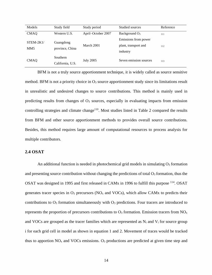
BFM is not a truly source apportionment technique, it is widely called as source sensitive
method. BFM is not a priority choice in O3 source apportionment study since its limitations result
in unrealistic and undesired changes to source contributions. This method is mainly used in
predicting results from changes of O3 sources, especially in evaluating impacts from emission
controlling strategies and climate change110. Most studies listed in Table 2 compared the results
from BFM and other source apportionment methods to provides overall source contributions.
Besides, this method requires large amount of computational resources to process analysis for
multiple contributors.
2.4 OSAT
An additional function is needed in photochemical grid models in simulating O3 formation
and presenting source contribution without changing the predictions of total O3 formation, thus the
OSAT was designed in 1995 and first released in CAMx in 1996 to fulfill this purpose 114. OSAT
generates tracer species in O3 precursors (NOx and VOCs), which allow CAMx to predicts their
contributions to O3 formation simultaneously with O3 predictions. Four tracers are introduced to
represents the proportion of precursors contributions to O3 formation. Emission tracers from NOx
and VOCs are grouped as the tracer families which are represented as Ni and Vi for source group
i for each grid cell in model as shown in equation 1 and 2. Movement of traces would be tracked
thus to apportion NOx and VOCs emissions. O3 productions are predicted at given time step and

15
locations in models, tracer families (O3Ni and O3Vi in Equation 3 and Equation 4) are generated
simultaneously to estimate the proportion of O3 formation to emissions of NOx and VOCs under
certain O3 regime scheme.
Equation 3 :
∑ 𝑁𝑖 = 𝑁𝑂𝑖 +𝑁𝑂2𝑖𝐼𝑖=1 , i=1, 2, 3…, I
Equation 4 :
∑ 𝑉𝑖 = 𝑉𝑂𝐶𝑠𝑖𝐼𝑖=1 , i=1, 2, 3…, I
Equation 5 :
∑ 𝑂3𝑁𝑖 + 𝑂3𝑉𝑖 = 𝑂3𝑖𝐼𝑖=1 , i=1, 2, 3…, I
OSAT is improved to advanced version to increase accuracy in calculating O3 contributions
from its sources by considering the feedbacks of reactions in O3 production and destruction.
Tagged atomic oxygen in predicted net O3 production are traced in deforming process, and O3
destruction rate due to reactions with species such as HOx (OH and HO2) helps to quantify the
potential O3 reformation. Such improvements were released in 2005 known as OSAT2 with
updated version of CAMx 115. A subsequent improvement (OSAT3) was released in 2015 along
with CAMx version of 6.3. The odd oxygen in chemical reactions of O3 reforming processes is
tagged with associated source groups, thus regenerated O3, NO and NO2 are evaluated. As results,
predicted O3N and O3V contain information of O3 reforming, and the accuracy of O3 source
apportionment is improved. This technique is commonly used in recent O3 source analysis,
summary of recent studies applying OSAT is listed in Table 3.
16
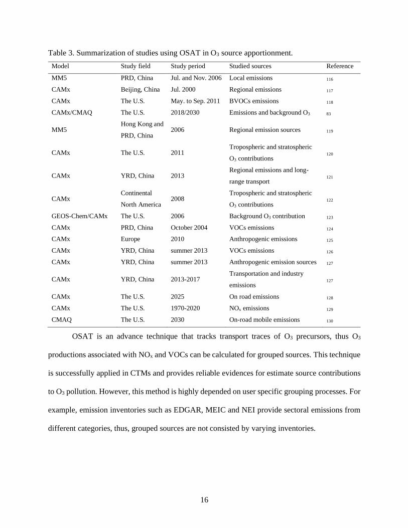
Table 3. Summarization of studies using OSAT in O3 source apportionment.
Model Study field Study period Studied sources Reference
MM5 PRD, China Jul. and Nov. 2006 Local emissions 116
CAMx Beijing, China Jul. 2000 Regional emissions 117
CAMx The U.S. May. to Sep. 2011 BVOCs emissions 118
CAMx/CMAQ The U.S. 2018/2030 Emissions and background O3 83
MM5 Hong Kong and
PRD, China 2006 Regional emission sources 119
CAMx The U.S. 2011 Tropospheric and stratospheric
O3 contributions 120
CAMx YRD, China 2013 Regional emissions and long-
range transport 121
CAMx Continental
North America 2008
Tropospheric and stratospheric
O3 contributions 122
GEOS-Chem/CAMx The U.S. 2006 Background O3 contribution 123
CAMx PRD, China October 2004 VOCs emissions 124
CAMx Europe 2010 Anthropogenic emissions 125
CAMx YRD, China summer 2013 VOCs emissions 126
CAMx YRD, China summer 2013 Anthropogenic emission sources 127
CAMx YRD, China 2013-2017 Transportation and industry
emissions 127
CAMx The U.S. 2025 On road emissions 128
CAMx The U.S. 1970-2020 NOx emissions 129
CMAQ The U.S. 2030 On-road mobile emissions 130
OSAT is an advance technique that tracks transport traces of O3 precursors, thus O3
productions associated with NOx and VOCs can be calculated for grouped sources. This technique
is successfully applied in CTMs and provides reliable evidences for estimate source contributions
to O3 pollution. However, this method is highly depended on user specific grouping processes. For
example, emission inventories such as EDGAR, MEIC and NEI provide sectoral emissions from
different categories, thus, grouped sources are not consisted by varying inventories.

17
2.5 Source-oriented methods
NOx and VOCs are regarded as main precursors of O3 formation, NO2 is formed through
the oxidation of NO by O3 while organic peroxy radicals (RO2) and hydroperoxy radicals (HO2),
which play important roles in forming O3 formation, are formed through reactions of VOCs131. O3-
oriented technique provides the detailed surface O3 source apportionment for multiple targets
(sources, regions and species) in single simulation in air quality models132, 133. This advanced
technique is developed to track O3 formation by tagging O3 precursors in their source emissions
while air quality model is conducting. As main precursor of O3, NOx emissions are always tagged
in this approach. Detail tagging method is briefly introduced in Zhang and Ying 134. Generally,
following reactions of Equation 6 and Equation 7, O3 formation from different sources can be
identified.
Equation 6:
NO2n+hv---NOn+O(3P)n, n=1,2,3…,N
Equation 7:
O(3P) n+O2---O3n, n=1,2,3…, N
In equation above, superscript n represents NOx emissions from source n, these functions
are added in air quality simulation so that O3 formation in simulation outputs show their source
tagged emissions.
As another main precursor, VOCs contributions to O3 formation is hard to evaluate since
their variety of components and intermediate reactions. As recorded in Ying and Krishnan 135,
reactions of a general reactive hydrocarbon (RH) from emission source n are tagged to tracking
VOCs contributions by following equation:

18
Equation 8:
RHn+HO—RO2n+H2O, n=1,2,3…, N
Equation 9:
RO2n+NO—NO2+ROn, n=1,2,3…, N
In these reaction processes, contribution of HO2 from emission sources can be directly
calculated and conversion rate (R) from NO to NO2 can be determined as F in following equations,
thus O3 apportionment can be estimated.
Equation 10:
Fn=R(NO2n)/R(NO2tot), n=1,2,3…, N
Equation 11:
O3n=Fn*O3tot, n=1,2,3…, N
R(NO2n) in Equation 10 represents conversion rate from source n, NO2tot represents overall
NO to NO2 concentration rate in all VOCs sources. O3tot is the predicted overall net O3 formation
rate. O3 contributions from VOCs emission sources can be calculated by applying above functions
in AQMs.
Based on source-oriented technique, O3 contribution from NOx and VOCs emissions can
be processed in single simulation, however uncertainties due to nonlinear photochemical reaction
rate which greatly varied from different NOx and VOCs concentration, multiple classification
schemes, such as NOx-sensitive, VOCs-sensitive, two-regime (2R) and three-regime (3R), are
applied in source oriented simulations to investigate O3 contribution from NOx and VOCs. In
following sections, these regime schemes will be brief reviewed.

19
2.6 O3 regime schemes
Four regime schemes are discussed in this section. These schemes are mostly used
independently in O3 simulation in which NOx or VOCs are determined as dominant precursor. In
case where NOx is determined as dominant precursor, O3 formation is attributed to NOx emission
only; similarly, the same idea for VOCs dominant regions. For example, Zhang and Ying 134
studied NOx contributions to O3 in Houston-Galveston-Brazoria (HGB) and Beaumont-Port Arthur
(BPA) in the U.S. were determined as NOx sensitive regions. However, it is hard to determine
whether O3 production generated in specific periods or regions is relative to NOx-sensitive or
VOCs-sensitive. 2R scheme is introduced to determine O3 attribution to NOx and VOCs. O3
production is attributed to either NOx or VOCs emissions based on O3 chemical formation regime.
Regime is classified by different indicator ratios. Kwok, et al.52 applied the ratio of production of
hydrogen peroxide to nitric acid, to determine if O3 product occurs in either NOx- or VOCs-
sensitive chemical regime. Besides, indicator ratio was set to 0.35 based on previous studies 136,
137. Some other indicators are also applied to identify O3 sensitivity to NOx and VOCs. Ratio of
H2O2/(O3+NO2), HCHO/NOy and HCHO/NOz were applied to determine VOCs-limited O3
formation with transit value of 0.02, 0.28 and 1, respectively138-141. Within these indicators,
production rate of H2O2/HNO3 is most widely recruited to identify O3 sensitivity to NOx and VOCs
as 2R in recent studies. A summary of recent studies that applied 2R in O3 source apportionment
analysis are listed in Table 4.
Table 4. Summary of studies using 2R scheme in O3 source apportionment
Model Study field Study period Study sources Reference
CAMx PRD, China Jun. 26–Jul. 2,
2000 NOx and VOCs emissions 142
(Table cont’d)

20
Model Study field Study period Study sources Reference
WRF-Chem Eastern China Summer 2011 Diurnal pattern and regional
sources
143
CCM/CHASER Japan 1980–2005 Regions of emission sources 144
CMAQ California, U.S. Jun. to Jul. 2007 Emissions of NOx and VOCs 52
CAMx YRD, China 2015 Emissions of NOx and VOCs 145
CAMx YRD, China Summer 2013 Emissions of NOx and VOCs 146
CAMX PRD, China 2006 Emissions of NOx and VOCs 147
Though 2R approach is mainly used as current O3 source analysis method, uncertainties
remain. A single threshold (ratio indicator) might not be sufficient since both NOx and VOCs
control O3 formation simultaneously. Thus, the transition regime is introduced to improve
measurement that O3 attribute to both NOx and VOCs. Thus, 3R scheme is improved to estimate
O3 contributions from transition regime. Based on analysis of O3 production efficiency and
formation kinetics136, production ratio of (H2O2+ROOH)/HNO3, as a widely used indicator, was
reevaluated based on 2R scheme in SAPRC photochemical mechanism in a model based
estimation 53. The transition regime is defined when ratio is between 0.047~5.142. 3R regime is
updated and validated in 2018, its ability in providing understanding of O3 attribution to NOx and
VOCs carried out a higher accurate result O3 contributions from its sources148.
2.7 O3 source apportionment in China
Severe O3 pollution is reported in previous studies in eastern China with high 8h-O3
concentration exceeding the Chinese National Ambient Air Quality Standard (CNAAQS) of 82
ppb (160µg/m3) especially in warm and dry summertime51. Many studies analyzed sources of O3
in China. Generally, a shifting trend from NOx-limited to VOCs-limited was observed in rural area
as the latitude increases, and NOx emissions were estimated as the dominant precursors in southern
China while rural regions in north China were classified as VOCs-sensitive area149. Surface O3
concentration in eastern China was more sensitive to photochemistry while the transport processes

21
dominate the O3 in western regions where the climate conditions such as cloud convections play
an important role in forming O3150. Biogenic emissions were listed as one of the major sources that
enhance O3 formation in southeast and east China, and it also shift the dominant precursor from
NOx to VOCs in these regions151, 152.
High O3 episodes were frequently observed in many Chinese areas such BTH region, YRD,
Sichuan Basin and PRD153, 154. Increasing O3 concentrations were proved to associated with growth
of NOx and VOCs emissions as the result from urbanization and economic development in recent
years. It is also revealed that high concentrations in summertime were due to on-road vehicles
emission of NOx and VOCs155. Research has focused on O3 and its source apportionment in high
risk areas to assess the dominant sources. Results are provided as solid evidence for making a
strategic policy to reduce O3 pollution in China.
It was reported that 8h-O3 concentration in YRD increased from 144 µg/m3 to 168 µg/m3
since 2013 to 2017. Emissions from industry and vehicle sectors were found to be as the major
sources127. Surface O3 in Shanghai was briefly analyzed since it was one of the biggest cities in
China located in YRD and suffered high summer O3 concentration by more than 300µg/m3 156. A
regional source apportionment study revealed that Shanghai was greatly affected by local emission
which account for ~28.9% of total O3. Contributions from emissions of surrounding regions also
caused significant increases of O3. Emissions from north Zhejiang provinces were estimated to
associate with ~19.9% of total O3 concentration in Shanghai 156, 157. Sectoral source apportionment
results revealed high contributions from industry (~39.2%), mobile source (~21.3%), biogenic
(~13.0%) and power plants (~7.1%) in Shanghai121. As one of major sources, biogenic emissions
of VOCs were estimated to contribute maximum of 36 µg/m3 O3 in YRD especially in rural area,
it also enhanced daytime O3 by maximum of ~15 µg/m3 158, 159.

22
PRD is another high-risk area where O3 is listed as the major air pollutant. High
concentration episodes were always observed in autumn at urban regions with maximum of > 100
ppb160, 161. Local emissions were evaluated cause more than 50% (maximum of ~70%) of total O3
formation, and mobile emission was the major source for high concentration episodes 116.
Emissions from central and west PRD were transported to south regions and induced high
concentration episodes with concentrations higher than 100 ppb under a low air pressure system
and slow south wind160. VOCs emissions were evaluated as dominant precursors in PRD, species
such as p-xylene, 1,2,4-trimethylbenzene, 2-methyl-2-butene, 1-butene and α-pinene were listed
as the dominant species. Besides, VOCs emissions were reported associate with ~64.1% of total
O3 formation potentials162, 163. Mobile source (40%) was also estimated as the major source of O3
followed by biogenic emissions (29%)164. An analysis in Guangzhou indicated a similar result of
contribution from mobile emission while the second source was industrial emission rather than
biogenic due to high urbanization and industrialization in this megacity165.
As one of most polluted regions, NCP is facing severe O3 pollution due to increasing
emissions of NOx and VOCs. Emissions from Hebei and Shandong provinces enhanced the O3
formation in summertime, which is always referred as the high concentration episode166. High O3
concentrations recorded in Beijing ranged from 80 to 159 ppb in urban area during summertime,
and the major source was estimated to NOx emissions especially those from urban area167, 168. O3
pollution in urban Beijing was also estimated due to emissions from Tianjin and the south Hebei
province169. Shandong was also reported to enhance O3 concentration in high concentration
episodes 170. Though O3 pollution in NCP is getting worse, there is insufficient data to fully analyze
O3 source apportionment in this region. Without solid evidence to quantify the effects from
emission sources, no effective controlling strategies could be implemented to reduce O3 pollution

23
in NCP; however increasing concern for this issue demands an improvement in air quality in
capital regions. Thus, greater effort should be put to analyze O3 and its source apportionment in
NCP.
2.8 Conclusions
Four main methods for O3 source analysis are reviewed in this chapter, and each approach
has their own limitations and advantages. As the source sensitive methods, DDM and BFM provide
limited information for source contribution from emissions. They miss information from complex
nonlinear chemical reactions and potential contributions from removed sources102. OSAT offers a
much more reliable and simpler way to estimate source contributions to O3. Tagged tracers help
to identify the source contributions. However, non-reactive tracers in this method limit its ability
to track source contribution during chemical reactions. An alternative method, the source-oriented
approach, clearly quantifies O3 contribution from its precursors. This method has a strong ability
in tracking O3 formation from non-linear chemical processes, O3 formation from NOx and VOCs
are involved. Thus, the tagged sources can be identified in simulation outputs. This method
overcomes limitations in methods mentioned above and has been widely accepted in recent O3
source apportionment studies. Though source-oriented approach has advantages in tracking
sources of precursors, limitations also existed. In most case, the study domain is not dominated by
single precursor, and is affected by seasons and regions. NOx- or VOCs-sensitive simulation might
not be able to provide accurate source apportionment. 2R scheme is introduced to fix this issue,
which solve most problem, but results would be varied due to application of different indicators.
O3 formations in “transition” regime also lead to uncertainties in 2R scheme. 3R is developed to
overcome this issue as it which offers higher accuracy results of contributions from NOx and VOCs
emissions.

24
Many studies analyzed O3 source apportionment in China and pointed out that emissions
from mobile vehicles, industry and biogenic cause high O3 concentration. O3 sensitivity to NOx
and VOCs were also analyzed. BVOCs was revealed to enhance O3 concentration significantly.
However, insufficient studies have been conducted to analyze O3 source apportionment in NCP
which is one of the most polluted regions in China. More attention should be put on this area. As
one of air pollutants, O3 leads to serious risk in human health and ecological lost. Efforts are needed
to improve accuracy in measuring O3 from complex non-linear photochemical processes, such as
evaluating a better regime indicator in 3R scheme for different locations. Choosing a reasonable
source apportionment method also makes sense in different simulation purposes. Although these
methods have their own limitations, they also provide realistic results in each study, which
contributes to a better understanding of O3 in the world.

25
CHAPTER 3. IMPROVING OZONE SIMULATION IN THE NCP
3.1 Introduction
Numerous studies have shown adverse environmental and public health impacts associated
with tropospheric O3 pollution 5, 171, 172. O3 exposure is associated with respiratory-related hospital
admissions, cardiovascular diseases, school day loss, asthma-related emergency department visits,
premature mortality, etc. 3-6. Fann, et al.13 revealed that 4700 deaths and 36,000 life-year losses
were due to long-term O3 exposure based on O3 concentration in 2005 across the continental United
States. In China, around 55 to 80 thousand mortalities in 2015 were attributed to chronic
obstructive pulmonary disease (COPD), and a total 816.04 million cumulative population was
estimated exposed to 8h-O3 concentrations (>100 μg/m3)14, 154. O3 level in 2000 also induced 6.4%-
14.9% yield loss of food crop, and estimated O3 concentration in 2020 would cause 47.4 million
metric tons loss of four grain crops produced in China 15.
Increasing O3 concentration were reported in many studies. Country scale statistical
analysis in 74 cities indicated that 8h- O3 increased from ~69 ppb in 2013 to 75 ppb in 2015, and
a 15% increase of non-compliant cities were also revealed with increasing O3 level in China 69.
An average increase rate of 1.13 ± 0.01 ppb/year of 8h- O3 was observed in north of eastern China
from 2003 to 2015, and total O3 variations were due to short-term (36.4%), seasonal (57.6%) and
long-term (2.2%) changes 16. About 50% of the days with O3 concentration exceeding 80 ppb in
Beijing-Tianjin region (maximum of 170 ppb) were reported during 1983-1986 173. Significant
increases were also observed in Mt. Tai with an average increase by 1.7 ppb/year in June and by
2.1 ppb/year in July to August during 2003-201517. Recent studies reveal that China is

26
experiencing severe O3 pollution, but O3 variations and its impact factors are not well studied.
Lacking comprehensive analysis leads to a challenge in lowering O3 pollution.
Chemical transport models (CTMs) are commonly used tools to understand the formation
and transport of O3. Li, et al.12 analyzed the impacts of chemical production and transport on
diurnal O3 behaviors in Mt. Tai and revealed that regional transport and chemistry production
contribute ~60 and ~25 ppb, respectively, in afternoon-maximum concentration in June 2006 based
on results obtained from the Nested Air Quality Prediction Modeling System (NAQPMS). Yang,
et al.23 applied global three-dimensional Goddard Earth Observing System chemical transport
model (GEOS-Chem) to analyze impacts of sulfate and nitrate on surface-layer O3 concentration
in China and indicated that sulfate dominates in O3 increases while nitrate dominates in O3
reductions. Hu, et al.24 simulated tropospheric O3 in the North China Plain (NCP) for 2015 summer
by applying the Community Multiscale Air Quality (CMAQ) model and found that emissions from
Shandong and Hebei make the largest contribution not only to the highest local O3 concentration
but also to Beijing and Tianjin. They also pointed out that most urban O3 pollutions are mainly
dominated by conditions sensitive to volatile organic components (VOCs), and figured out that
emission control strategies in industry, residential and power plant sectors would make significant
effects on reducing O3 concentration. Though O3 is receiving increasing attention, limited
understanding of its variation and impacts require comprehensive analysis in China specially in
the NCP 16, 17, 174, 175.
CTMs are very useful for understanding O3, but the accuracy is highly dependent on
emission inventories. Several emission inventories covering China and surrounding regions are
available for different simulation purposes37, 38. Inventories from regional to continental scales, for
different pollutant species and emission sectors 39-43 32 were created and were successfully applied
27
in O3 simulation in China, including Emission Database for Global Atmospheric Research
(EDGAR), Multi-resolution Emission Inventory for China (MEIC) and Regional Emission
inventory in ASia (REAS) 44-48. However, to a large extent, these inventories are not entirely from
bottom-up, leading to large uncertainties in simulation results 50. EDGAR and MEIC are two most
widely used inventories in China, while their performances in O3 simulation vary in years and
regions 41, 51. Evaluating and improving their performance in O3 prediction would provide
convincing results for deeper understanding of O3 formation, health risks, and design of controlling
strategies.
This study applies the CMAQ model to estimate the pollution level and health risks of O3
in the NCP during summer 2017 with the anthropogenic emission inventories of MEIC and
EDGAR+ (improved version of EDGAR). O3 variations and the impacts from meteorological
conditions and precursors emissions are discussed in detail.
3.2 Methods
3.2.1 Model description
O3 concentrations are simulated using the CMAQ model v5.0.1 176, 177 in 12km×12km
horizontal resolution domain (Figure 1) that covers NCP including Beijing, Tianjin, Hebei,
Shandong, part of Henan, Jiangsu, Anhui and Inner Mongolia (note that the map is generated by
using NCAR Command Language (NCL) 178). Initial and boundary conditions are both generated
by simulation on coarse domain (36 km ×36 km) which covers mainland China and part of
surrounding countries. Photochemical mechanism SAPRC-11177 and aerosol chemistry
mechanism AERO6 179 are used. The Weather Research and Forecasting (WRF) v 3.7.1177, 180, 181
model is applied to generate meteorological inputs with initial and boundary conditions from
National Centers for Environmental Prediction (NCEP) FNL (Final) Operational Global Analysis

28
data (http://dss.ucar.edu/datasets/ds083.2/)181, 182. Meteorology-Chemistry Interface Processor
(MCIP) v4.2 is applied to convert WRF outputs into CMAQ ready meteorological inputs. Different
anthropogenic emission inventories are re-gridded to designed domain by using the Spatial
Allocator 183. The Model for emissions of Gases and Aerosols from Nature (MEGAN) 184 is used
for biogenic emissions and the Fire Inventory from NCAR (FINN) 185 provides biomass burning
emissions.
Figure 1. Simulation domains. Coarse domain (36km by 36km) covers mainland China and part
of surrounding countries. NCP (d02) is included as the finer domain (12km by 12km).
3.2.2 Case description
3.2.2.1 EDGAR+ inventory
As precursors of O3 production NOx and VOCs play important roles in O3 simulation. Two
anthropogenic emission inventories with modified NOx and VOCs are applied in this study for

29
comparison. In first scenario, which is referred as “EDGAR+” hereinafter, anthropogenic
emissions of VOCs and NOx from EDGAR 186 for China are scaled to 2012 (off-road), 2015
(industry, residential, on-road and energy), and 2016 (industry, residential, on-road and energy for
Beijing) to represent as in 2017. Scaling factors for VOCs and NOx are shown as in Table 5 and
Table 6. On-road emissions are scaled down to the national total given for 2017 in China
Vehicle Environmental Management Annual Report
(http://dqhj.mee.gov.cn/jdchjgl/zhgldt/201806/P020180604354753261746.pdf). Emissions from
energy, residential and industry sectors are scaled down from KNMI (Royal Netherlands
Meteorological Institute) DECSO (Daily Emission estimates Constrained by Satellite
Observation) based on Ozone Monitoring Instrument (OMI) data 187, 188 to match year-on-year
reduction rate given for 2016 (4%) and 2017 (4.9%) in Government Working report. NOx
emissions in off-road and agriculture remain as in 2012 since there is not enough evidence to
determine scaling factors for them.
Table 5. Scaling factors for VOCs emissions in NCP
Agriculture Residential Industry Energy On-road Off-road
Beijing 3.64 0.08 1.13 1.19 1.59 1.39
Tianjin 21.87 0.04 4.31 2.90 0.67 7.44
Hebei 44.78 0.46 1.25 2.92 2.88 4.41
Shandong 22.39 0.40 1.58 4.16 2.39 3.58
Shanxi 37.78 0.42 0.24 2.62 2.17 3.57
Henan 13.75 0.46 1.07 2.24 3.09 2.01
Jilin 175.52 0.59 2.31 3.23 2.67 0.59
Liaoning 36.32 0.36 0.80 4.17 2.62 7.32
Heilongjiang 116.51 1.12 1.07 2.23 2.74 0.36
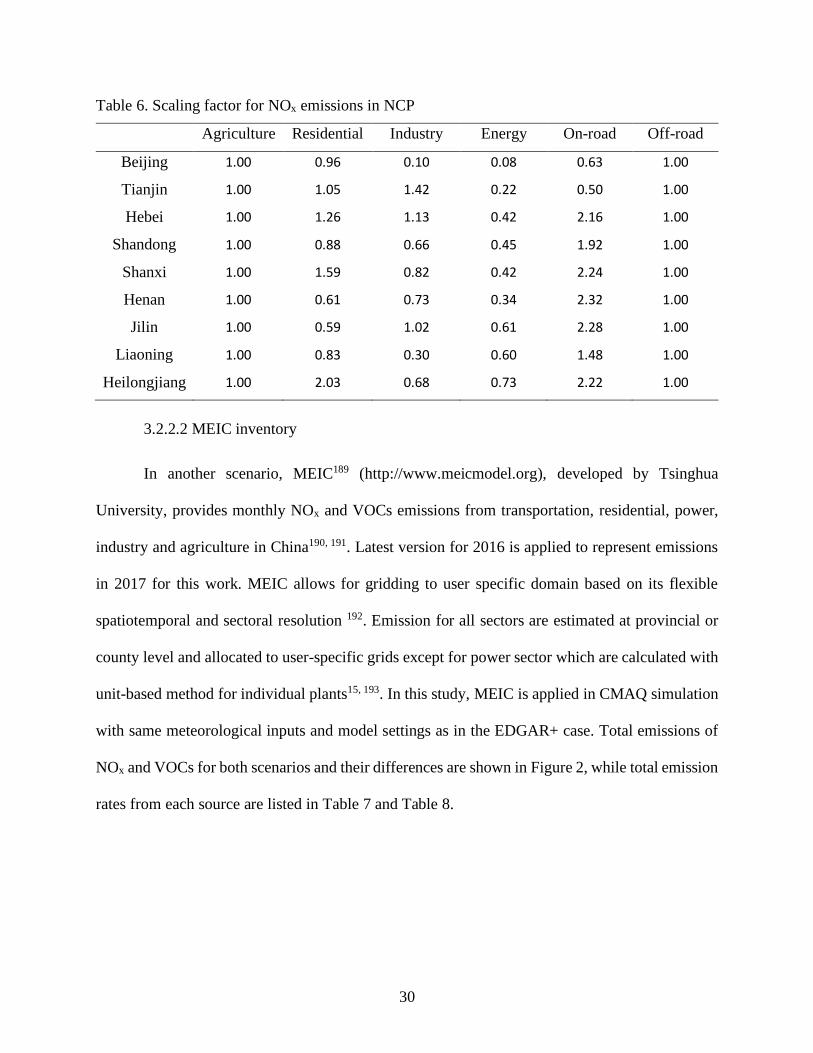
30
Table 6. Scaling factor for NOx emissions in NCP
Agriculture Residential Industry Energy On-road Off-road
Beijing 1.00 0.96 0.10 0.08 0.63 1.00
Tianjin 1.00 1.05 1.42 0.22 0.50 1.00
Hebei 1.00 1.26 1.13 0.42 2.16 1.00
Shandong 1.00 0.88 0.66 0.45 1.92 1.00
Shanxi 1.00 1.59 0.82 0.42 2.24 1.00
Henan 1.00 0.61 0.73 0.34 2.32 1.00
Jilin 1.00 0.59 1.02 0.61 2.28 1.00
Liaoning 1.00 0.83 0.30 0.60 1.48 1.00
Heilongjiang 1.00 2.03 0.68 0.73 2.22 1.00
3.2.2.2 MEIC inventory
In another scenario, MEIC189 (http://www.meicmodel.org), developed by Tsinghua
University, provides monthly NOx and VOCs emissions from transportation, residential, power,
industry and agriculture in China190, 191. Latest version for 2016 is applied to represent emissions
in 2017 for this work. MEIC allows for gridding to user specific domain based on its flexible
spatiotemporal and sectoral resolution 192. Emission for all sectors are estimated at provincial or
county level and allocated to user-specific grids except for power sector which are calculated with
unit-based method for individual plants15, 193. In this study, MEIC is applied in CMAQ simulation
with same meteorological inputs and model settings as in the EDGAR+ case. Total emissions of
NOx and VOCs for both scenarios and their differences are shown in Figure 2, while total emission
rates from each source are listed in Table 7 and Table 8.

31
Figure 2. Averaged NOx and VOCs emission rates from MEIC and EDGAR+ and their
differences (subtracting EDGAR+ by MEIC) in summer 2017. Units are tons/month.
Table 7. NOx emission from each source for different inventory in NCP 2017 summer.
MEIC (104 ktons/month) EDGAR+ (104 tons/month)
Agriculture NA Agriculture 6.19
Residential 4.18 Residential 3.57
Power 60.73 Energy 38.58
Industry 106.34 Industry 53.41
Transportation 83.05 On-road 38.10
NA NA Off-road 12.32
Total 254.30 Total 152.16
Table 8. VOCs emission from each source for different inventory in 2017 summer.
MEIC (103 ktons/month) EDGAR+ (103 ktons/month)
Agriculture NA Agriculture 1.90
Residential 4.21 Residential 3.15
Power 0.11 Energy 0.35
(Table cont’d)

32
MEIC (103 ktons/month) EDGAR+ (103 ktons/month)
Industry 24.77 Industry 16.15
Transportation 6.50 On-road 5.66
NA NA Off-road 0.29
Total 35.58 Total 27.50
3.4 Results and discussions
3.4.1 Overall performance
Predicted meteorological conditions (temperature (T), wind speed (WS), wind direction
(WD) and relative humidity (RH)) from WRF for the simulation period are validated using
observed data from National Climate Data Center (NCDC, https://www.ncdc.noaa.gov/). A total
of 108 stations are involved. The mean bias (MB), gross error (GE) and root mean squared error
(RMSE), as well as mean observation (OBS) and prediction (PRE) of meteorological parameters
are shown in Table 9. Statistical results are compared with benchmarks from Emery, et al. 194.
Generally, WRF slightly over-predicts temperature and wind speed but underestimates RH in
summer. Uncertainties of these biases are believed to result from the model itself including domain
resolution, model configuration and parameterization195. Though biases exist, predictions from
WRF are normally accepted in previous work over China with similar statistical results 196, 197.
Table 9. Summertime model performances of meteorological conditions in NCP for temperature
(T), wind speed (WS), wind direction (WD) and relative humidity (RH). T (℃) WS (m/s) WD (⁰) RH (%)
OBS 24.32 3.27 168.99 63.41
PRE 25.35 3.82 169.89 58.40
MB 1.03 0.56 1.71 -5.01
RMSE 2.72 1.85 58.51 15.3
GE 2.04 1.42 41.89 11.79
1. Benchmark of MB for T, WS and WD is ±0.5, ±0.5 and ±10, respectively.
2. Benchmark of GE for T, WS and WD is 2, 2 and 30, respectively.
3. Benchmark of RMSE for WS and WD is 2 and 30, respectively.

33
8h-O3 observations from CNEMC are used to validate model performance on O3. Table 10 shows the comparison of model and
predicted concentrations in 11 major cities in the NCP from June to August 2017, together with statistics including averaged observations
(OBS), averaged predictions (PRE), the mean fractional bias (MFB), the mean fractional error (MFE), the normalized mean error (NME)
and the normalized mean bias (NMB). For cities with multiple monitoring stations, averaged concentrations are applied. Different cutoffs
for O3 (from 40 to 60 ppb) are used to analyze the performance of the model as suggested by the US EPA198. In this study, 8h-O3
concentrations higher than 30 ppb are included in analysis based on a previous study 199.
Table 10. Model performances in 11 major cities in NCP for 8h-O3 simulation using EDGAR+ (E) and MEIC (M). Units are ppb for
OBS and PRE. Bold represents the statistical result exceeds criteria. City Baoding Beijing Datong Hohhot Jinan Shijiazhuang Taiyuan Tangshan Tianjin Xuzhou Zhengzhou
OBS 83.13 71.98 63.14 67.53 71.26 72.21 72.38 73.24 70.60 70.71 78.84
PRE (M) 78.17 80.62 65.17 63.76 71.77 79.10 67.99 51.47 68.19 65.08 74.3
PRE (E) 73.98 75.35 62.06 61.55 68.51 79.45 69.68 65.83 62.55 62.73 73.75
MFB (M) -0.05 0.11 0.05 -0.05 0.03 0.09 -0.05 -0.4 -0.15 -0.07 -0.06
MFB (E) -0.09 0.09 -0.03 -0.11 -0.01 0.06 -0.09 -0.17 -0.21 -0.06 -0.05
MFE (M) 0.20 0.25 0.14 0.16 0.17 0.23 0.19 0.49 0.40 0.21 0.16
MFE (E) 0.15 0.29 0.14 0.15 0.18 0.16 0.14 0.29 0.3 0.22 0.13
NME (M) 0.20 0.32 0.17 0.15 0.19 0.26 0.20 0.39 0.39 0.21 0.15
NME (E) 0.14 0.34 0.15 0.14 0.19 0.17 0.13 0.26 0.26 0.22 0.12
NMB (M) -0.02 0.20 0.09 -0.03 0.06 0.15 -0.02 -0.27 -0.01 -0.03 -0.04
NMB (E) -0.07 0.17 -0.01 -0.09 0.02 0.09 -0.08 -0.12 -0.15 -0.03 -0.04

34
Figure 3 and Table 10 indicates that simulations for each inventory generally agree well
with observed O3 concentrations in NCP. MEIC always predicts higher O3 concentration than
EDGAR+ except in Tangshan and Taiyuan. Over-predictions occur in Beijing, Datong, Jinan and
Shijiazhuang for MEIC. It is noted that significant exceedances are observed in Beijing and
Shijiazhuang for MEIC. On the other hand, EDGAR+ usually under-predict O3 in this period. The
NMB in most cities match the US EPA criteria 200 of ±0.15 except in Tangshan for MEIC. Similar
outcomes are observed in the NME. The NME for both scenarios generally agree well with US
EPA suggested criteria of 0.25 200 , but there are 3 and 1 exceedances for MEIC and EDGAR+,
respectively. It is noted that the only exceedance in EDGAR+ is 0.29 (Tangshan), but 3
exceedances are observed in MEIC with one extreme case (Tangshan, 0.32). The MFB and MFE
in EDGAR+ match suggested criteria of ±0.15 and 0.35 200 with only one slight exceedances in
Tangshan (MFB of -0.16). The MFB and MFE for MEIC also indicates that model results meet
performance goals in most cases except in Tangshan where both indices are not within suggested
criteria. Based on statistical results, EDGAR+ has better performance in major cities in NCP.
These major cities generally represent the air quality in the NCP, thus, both inventories result in
satisfactory model performances and are reliable for further analysis in this study. Though
uncertainties of O3 simulation are associated with meteorological field, emissions, model treatment,
and configurations 199, statistical results indicate the CMAQ model is capable of estimating
short/long term O3 concentrations variations and effects in NCP.

35
Figure 3. Model performance statistics on average daily 8h-O3 concentration. Summertime
average concentration (top), MFB, MFE, NME and NMB for 11 major cities are shown. Red
lines represent suggested criteria by US EPA for each index.
3.4.2 Temporal and spatial variations
Figure 4 illustrates the comparison of averaged daily 8h-O3 concentration from prediction
and observation in 8 major cities in NCP from June to August in 2017. Generally, predicted
concentration from EDGAR+ and MEIC agree well with observation. Results from both
inventories successfully match the absolute level and temporal variations in major cities, even
though biases occur in specific period. It is noted that predictions in late June and early July are
mostly lower than observations for most cities (except Shijiazhuang and Zhengzhou) especially

36
when O3 concentration is higher than 100 ppb. Unexpected biases exist for many reasons such as
uncertainties in meteorological conditions, inventories and model treatment and configuration 177.
In Beijing, under-predictions (~30 ppb) also occur in the beginning of August when O3
concentrations are ~120 ppb. Over-predictions are observed in late July and early August and part
of late August exceeding > 40 ppb. This uncertainty may due to uncertainties in precursor’s
emission (such as NO, NO2 and VOCs) inventories 201. Simulation in Tianjin indicates that
EDGAR+ has higher accuracy in June and July but fail in matching variations in early August.
MEIC yields similar predictions before mid-July but result in under-predictions in late July, and it
shows a better performance in August than EDGAR+. There are clear differences between
EDGAR+ and MEIC in Shijiazhuang before end of July, with MEIC predicting significantly
higher concentration (10~30 ppb) than EDGAR+. Both inventories over-predict by ~50 ppb on
around July 22nd. Over-predictions are also observed in Jinan during the same period. Another
significant over-prediction is observed in Xuzhou at the end of July and beginning of August where
the observation is lower than 60 ppb. Simulations in Hohhot generally agree well with observation
except two significant under-prediction periods (late June to early July and early August).
Zhengzhou also has great agreement with observation except that specific extreme bias occurs in
middle June and early August. Generally, EDGAR+ and MEIC predict similar O3 concentration,
and MEIC predicts slightly higher concentration than EDGAR+ in most cities. Comparison
between observations and model predictions help to point out that EDGAR+ has better predictions
in summertime at most cities.

37
Figure 4. Average daily 8h-O3 concentration in major cities. Results from EDGAR+ (E) and
MEIC (M), observation (Obs) and statistical results (NMB) are shown in each row. Units for O3
concentrations are ppb.
Average diurnal variation of 8h-O3 concentration and corresponding meteorological
conditions are shown in Figure 5. In Beijing, MEIC predicts significant higher concentration (~10
to 20 ppb) before noon time (12:00 pm) and lower after 15:00 pm till the sunrise in the next day
38
compared with observation data while over-predictions in EDGAR+ are lower (~5 to 10 ppb) than
MEIC during the day time compared with MEIC. Both EDGAR+ and MEIC over-predicts the
peak value before noon time. In Beijing, EDGAR+ shows a higher sensitivity to temperature since
peak concentrations are predicted when the temperature is also high while MEIC always predicts
peak concentration ~2 hours ahead of EDGAR+. MEIC and EDGAR+ have similar performance
in predicting concentration in Hohhot, and MEIC always predicts ~5 to 10 ppb higher
concentration during the nighttime than EDGAR+. In Hohhot, MEIC and EDGAR+ always predict
peak values at a similar time around noon time to afternoon (12:00pm – 18:00 pm) and agree well
with the observations. MEIC predicts higher concentration during morning to noon time in Jinan,
and a significant bias can be observed between MEIC and observation data. In contrast, EDGAR+
has a better accuracy in matching the daily peak value as well as daily variations in Jinan.
EDGAR+ predicts lower concentration by ~5 to ~10 ppb in Shijiazhuang then MEIC while both
inventories always over-predict peak concentration by ~10 ppb compared to observation data
during noon time. Significant under-predictions of ~10 to 20 ppb are observed using both
inventories at nighttime. Predictions in Tianjin indicate that both inventories perform well in
matching the peak concentration around noon time (12:00 pm) while significant under-predictions
are observed at nighttime with a maximum by more than 30 ppb before sunrise (~4:00 am).
Predictions in Zhengzhou indicate that MEIC and EDGAR+ yield slightly over-estimates (5 ppb
and 10 ppb for EDGAR+ and MEIC, respectively) O3 concentration in daytime while significantly
under-predicting (~10 ppb lower) at night. MEIC predicts ~5 ppb higher O3 concentration in
daytime when EDGAR+ match well with observation data in Xuzhou. However, EDGAR+ has a
lower accuracy in predicting concentration before 6:00am, in which MEIC matches well with
observed concentration.

39
Figure 5. Diurnal variations of 8h-O3 from EDGAR+, MEIC and observation (Obs), temperature
(T) and relative humidity (RH) in major cities, Units for O3 concentration are ppb, for T are ˚C,
for RH are %.

40
Generally, MEIC predicts a slightly higher (~5 ppb) concentration than EDGAR+ before
noon time (12:00 pm) but not higher or even lower when the temperature is high, and RH is at a
low value in the afternoon. It is noted that both inventories predict O3 peak value well or only
slightly higher (< 5 ppb) in diurnal variations. In nighttime, the model predicts lower concentration
especially the time before 6 am. In other words, model has better performance in daytime.
Variations in all cities indicate that O3 concentrations are greatly affected by RH and temperature.
Diurnal variation also reveals that high O3 concentration is correlated to high temperature and low
RH. In the meantime, it also provides valid evidence that EDGAR+ has a higher accuracy in
predicting O3 concentration in NCP.
Figure 6 shows the spatial distribution of averaged 8h-O3 concentrations in the summer for
MEIC and EDGAR+ and their differences. Overall, O3 concentration increases from inner land to
coastal area, from rural to urban area and around major cities in each province. For both inventories,
high O3 concentrations occur at Beijing, Tianjin, Hebei, coastal Shandong and Jiangsu and junction
regions between Hebei, Shanxi and Henan with >100 ppb. It is noted that O3 concentrations are
also very high on surface of Bohai Sea with ~90 ppb. Concentrations in the rest of area range from
~60 to 80 ppb. Compared to MEIC, EDGAR+ predicts higher concentrations in eastern Tianjin,
western Hebei, Qingdao and Yantai by ~10 ppb but lower concentration in the rest region,
especially in Beijing, northern Shandong and southern Jiangsu by >10 ppb. Generally, MEIC
predicts slightly higher O3 concentrations in most of NCP and ocean surface above the Bohai Sea
while EDGAR+ results in higher predictions in part of major cities. The differences between two
scenarios are mainly due to emissions as shown in Fig 1. Higher emissions in MEIC induce higher
O3 concentrations in NCP, but since the O3 formation is not a linear reaction from NOx and VOCs,

41
higher O3 concentration in EDGAR+ is also due to lower emissions in specific regions such as in
western Hebei province. Detailed analysis will be discussed in following sections.
Figure 6. 8h-O3 concentrations in NCP for 2017 summer predicted by EDGAR+ and MEIC, and
their differences (subtracting EDGAR+ by MEIC). Units are ppb.
3.4.3 Peak episodes
There are 3 peak episodes observed during the simulation period including June 14th to 21st,
June 22th to 29th and July 8th to 15th (Figure 7). O3 variations in 8 major cities for these episodes
are analyzed. Hourly 8h-O3 in Figure 7 indicate the variation during peak episodes, in which peak
daily 8h-O3 concentrations are >100 ppb. In Beijing, peak values for each episode are ~120 ppb.
Simulation results in June are mostly slightly lower than observation data while over-predictions
on June 19th and July 11th with ~30 and 50 ppb higher than peak value, respectively, are shown in
S4 and S6 for MEIC. On the other hand, predictions from EDGAR+ match better in these episodes
with bias less than ±20 ppb. The model has higher accuracy in predicting high concentrations in
Tianjin compared with in Beijing. Most peak values match well with observation as shown in S4
and S5 except on June 14th to 16th when under-prediction occurs in both scenarios. It is noted that
over-prediction also existed on June 23rd and July 9th though part of observation data is missing
for these days. Peak concentrations are also caught in Shijiazhuang except on June 27th. EDGAR+
42
and MEIC match high concentration during peak episode, but they also over-predict on some days
such as June 15th, June 18th, June 26th and July 14th. The peak value on June 15th in Jinan is under-
predicted. From July 8th to 15th, simulations mostly agree well with observed concentration with
maximum bias on July 10th with around 15-20 ppb. Simulations in Hohhot indicate that predictions
from MEIC correspond much more closely to the peak concentration in the study. Similar situation
also occurs in Zhengzhou that peak concentrations are matched well on June 25th and July 10th but
not on June 20th when prediction are ~20 ppb lower. Peak concentrations are under-predicted in
Datong on June 15th, 28th and July 13th while predictions during the other peak episodes match
well and slightly higher than observations except on June 16th where the simulation results are
extremely higher. Spatial plots of 8h-O3 concentrations in 3 episodes (Fig. 6) indicates that
EDGAR+ predicts higher 8h-O3 than MEIC in most regions especially in west Hebei and the Bohai
Sea (~10 to 30 ppb) but lower in some major cities such as Beijing, Tianjin, Shijiazhuang and
Jinan by 10 ppb.

43
Figure 7. Hourly 8h-O3 concentration at major cities for peak episodes. Units are ppb.

44
Compared with averaged summertime differences in
Figure 8, EDGAR+ predicts a higher concentration during peak episodes although its emissions
of O3 precursors are lower than those in MEIC. High concentrations occurring during these
episodes might be due to specific climate conditions and emissions. Figure 9 shows climate
conditions (average temperature (T), relative humidity (RH), wind speeds (WS) and wind
directions (WD)) in 3 episodes. Spatial variation of meteorological conditions indicates that high
O3 concentrations always occur in locations where the temperature is higher than in the
surrounding region such as in south Hebei and north Henan. Low relative humidity and slow
wind speed are also observed in these regions to be associated with high O3 concentration. It is
obvious that high temperature, low RH and steady low air flow conditions are associated with
high O3 production in NCP. However, the opposite situation occurs in Bohai sea where
temperature is lower than surrounding area with higher RH and WS. After comparison, it is
noted that wind direction has less influence on O3 production then other variables.

45
Figure 8. Spatial distribution of 8h-O3 concentrations in 3 peak concentration episodes predicted
by EDGAR+ and MEIC, and their differences (subtracting EDGAR+ by MEIC). Units are ppb.

46
Figure 9. Meteorological conditions in NCP during 3 peak episodes. T represents temperature,
RH represents relative humidity, WS represents wind speed, red arrows in the third row represent
wind direction, arrow length represents wind speed.
Besides meteorological conditions, emission of O3 precursors also help to explain high
concentration occurrences in NCP. Figure 2 (right panel) shows the differences in NOx and VOCs
emissions between EDGAR+ and MEIC which are associated with differences in O3
concentrations in these periods. As emissions are generated using weekly data so the emissions in
three peak episodes are same (for five workdays and two weekend days). Significantly lower NOx
emission is noticed in south Hebei, north Henan and northwest and west Shandong in EDGAR+
47
while VOCs emission in these regions are not significant lower or ever higher than MEIC. High
O3 concentration in central NCP could mainly be due to NOx emissions. lower NOx leads to high
O3 concentration when VOCs emission is not too low. However, in Beijing and Tianjin, both NOx
and VOCs emissions in EDGAR+ are lower than in MEIC. As a result, EDGAR+ predicts lower
O3 in these regions. In south Shandong province, lower NOx emission with higher VOCs emission
barely change O3 formation in these regions. Overall, since O3 concentration is greatly dependent
on emission of precursors, changes of NOx and VOCs would influence O3 concentration in
different direction. Compared to MEIC, significantly lower (>200 tons/month) of NOx and similar
(difference within 5 tons/month) VOCs emissions in EDGAR+ induce more O3 formation; less O3
is predicted when both NOx and VOCs emissions are significantly lower (>200 tons/month
and >10 tons/month, respectively); O3 concentrations are barely changed (within ±10 ppb) when
NOx emissions are significantly lower (>200 tons/month) and VOCs emissions are significantly
higher (>10 tons/month) in EDGAR+. Due to nonlinear reactions of O3 formation, NOx and VOCs
play different roles in forming O3 under different conditions. It is concluded that a higher
concentration is always associated with slight lower emission under high temperature, low RH and
steady wind field. Though there might be some other reasons that could explain O3 concentration
variations such as solar radiation, cloud accumulation and concentration of particular matters (PM),
analyzing impacts from changes of emissions and meteorological conditions helps to figure out
the relationship between O3 and its impact factors, which will provide deeper understanding of
their impacts on forming and transporting O3. It is also offered as evidence for designing strategies
and policies to reduce O3 pollution.

48
3.5 Conclusions
The WRF/CMAQ modeling system is applied to simulate O3 concentrations in the NCP
during summer 2017 and the results using EDGAR+ and MEIC are compared. Generally, both
emission inventories perform well in predicting O3 concentrations in major cities. Statistical
metrices indicate that EDGAR+ performs better with fewer and smaller exceedances of suggested
performance criteria compared to MEIC. EDGAR+ is slightly better in representing overall
concentrations in NCP while MEIC shows better ability in predicting peak daily 8h-O3
concentrations. EDGAR+ also shows higher accuracy in matching O3 concentration in daytime.
NOx and VOCs emissions play different roles in forming O3 under different conditions, and high
concentrations are always associated with slightly lower emissions under high temperature, low
RH and steady wind field.

49
CHAPTER 4. OZONE SOURCE APPORTIONMENT IN THE NCP
4.1 Introduction
With its adverse impacts on human health, ground-level O3 is receiving increasing attention
in recent years in China14, 15, 69. As one of the most polluted regions in China, the NCP is facing
severe O3 issues. A report pointed out that more than 50% of the days O3 concentrations were
higher than 80 ppb during 1983-1986 in central NCP (Beijing-Tianjin-Hebei region) with peak
value of 170 pp173. Many studies also provided evidence that O3 concentration increased from
1980 to 2003, with peak mixing ratio to be up to 286 ppb in Beijing in 2005174, 175, 202. A long-term
station recorded O3 concentration in the NCP also indicated an increase of 1.13 ppb/yr during
2003-2015203. Both long- and short-term analysis in the NCP show the increasing trend of O3
concentration but not enough studies have analyzed O3 and its sources. Thus, comprehensive
analysis is necessary to better understand the impact factors and source of O3 formation in this
area.
Chemical transport models (CTMs) are widely used to simulate O3 and understand its
sources and impact factors. Source apportionment of O3 is very important to quantify source
contributions, which helps to design control strategies. But complex nonlinear reactions of O3
precursors, nitrogen oxides (NOx) and volatile organic compounds (VOCs), make it a challenge
for model simulation. To determine O3 contributions from NOx and VOCs, ratios of photochemical
chain reaction production rates, widely known as regime indicators, are introduced to classify O3
contribution. Traditional two regime (2R) approach was implemented in the Community Multi-
scale Air Quality (CMAQ) model 52 by applying indicator ratio of H2O2/HNO3 with correlation
coefficients ranging from 0.58 to 0.99. An improved method applied production ratio of

50
(H2O2+ROOH)/HNO3 as the indicator in three regime scheme (3R) was introduced into CMAQ 53
and compared with traditional 2R method, and results indicated higher contributions from NOx in
high O3 concentration regions in China by 5 to 15 ppb. 3R scheme was shown to provide more
accurate O3 contribution from its precursors53. Traditional O3 Source Apportionment Method
(OSAT) uses non-reactive tagged tracers in transport and reaction processes to track O3 sources
by splitting the concentration changes based on emission ratios33. An improved source-oriented
method that applied in CMAQ using reactive-tracers in all processes are also used in O3 source
apportionment34-36. O3 formation is strongly sensitive to concentrations of precursors, and its
source contributions are varied spatiotemporally, thus improved source apportionment technique
is necessary for more accurate results. In this study, improved source-oriented version of CMAQ
combined with 3R scheme will be applied in simulating O3 contribution from its precursors.
Due to the ability in irritating respiratory and cardiovascular system, O3 causes cough,
asthma, lung function reduction and other diseases. It was reported that 0.52% and 0.64% increases
of daily mortality and cardiovascular/respiratory mortality are associated with 10 ppb increase of
weekly O3 concentration 204. It was also reported that 10 μg/m3 increases of 8h-O3 were related to
0.42%, 0.44% and 0.50% increases of non-accidental mortality, cardiovascular mortality and
respiratory mortality, respectively, in China205, 206. However, there are inusfficient studies focusing
on O3 source attribution to these human health risk.
This study will quantify O3 contribution to sectoral/regional emissions of NOx and VOCs
by using source-oriented version CMAQ model with improved 3R scheme in NCP. Regional and
city-scale analysis provide a comprehensive understanding of source impacts in high O3
concentration season. Results from this chapter would provide O3 source contribution for further
analysis of O3 impacts on human health, economic benefits and ecosystem.

51
4.2 Methods
4.2.1 Model description
O3 concentrations are simulated by applying the CMAQ model (version of 5.0.1) with
AERO6 aerosol chemistry mechanism and SAPRC99 photochemical mechanism179, 207. The
Weather Research and Forecasting (WRF) version of 3.7.1 generates meteorological inputs by
using initial condition (ICs) and boundary conditions (BCs) from WRF preprocessing system
(WPS), which applies FNL operational global analysis data from National Center for Atmospheric
Research (NCAR, http://dss.ucar.edu/datasets/ds083.2/). Meteorological inputs are converted to
CMAQ ready format by using Meteorology-Chemistry Interface Processor (MCIP) v4.2. In this
study, improved Emission Database of Gas and Atmospheric Research (EDGAR+), which is
validated in previous chapter, provides anthropogenic emissions from sources of agriculture,
residential, energy, industrial, off-road and on-road. Biogenic emissions are provided by the Model
for Emissions of Gases and Aerosols from Nature (MEGAN) 184, and Fire Inventory from NCAR
(FINN) 185 is used to generate open-burning (wildfires) emissions. NOx and VOCs emission from
these sectors in NCP are shown in Figure 10 and Figure 11.

52
Figure 10. Averaged sources of NOx emissions in NCP 2017 summer. Units are tons/month.
Figure 11. Averaged sources of VOCs emissions in NCP 2017 summer. Units are tons/month.
Tagged tracers are introduced into source-oriented version CMAQ in this work, which have
been successfully applied in many previous studies134, 208, 209. Generally, atomic oxygen (O(3P))
that created in photochemical reaction between O3 precursors are tagged for each emission sources
following reactions, which are recorded in previous works 135.
Equation 12:
𝑁𝑂2𝑛ℎ𝑣→ 𝑁𝑂𝑛 + 𝑂(3𝑃)𝑛 , 𝑛 = 1,2,3… , 𝑁

53
Equation 13:
𝑂(3𝑃)𝑛 + 𝑂2 → 𝑂3𝑛 , 𝑛 = 1,2,3… , 𝑁
Equation 14:
𝑅𝐻𝑛 + 𝐻𝑂 → 𝑅𝑂2𝑛 + 𝐻2𝑂, 𝑛 = 1,2,3… ,𝑁
Equation 15:
𝑅𝑂2𝑛 +𝑁𝑂 → 𝑁𝑂2𝑛 + 𝑅𝑂𝑛 , 𝑛 = 1,2,3… , 𝑁
Where n represents the identification number of emission source, N represents total number
of emission sources. NO2 and NO are tagged for tracking NOx attribution while reactive
hydrocarbon (RH) are tagged for VOCs. Contribution rate (R) from NO to NO2, which is from
attribution of RO2, can be calculated and presented as O3 contribution from VOCs as shown in
Equation 16 and Equation 17. Fn represents contribution from source n, and O3tot in this equation
stands for net O3 formation predicted in model. O3 contribution from source n can be calculated
following Equation 17 by adding these functions in air quality models.
Equation 16:
𝐹𝑛 =𝑅(𝑁𝑂2𝑛)
𝑅(𝑁𝑂2𝑡𝑜𝑡), 𝑛 = 1,2,3… , 𝑁
Equation 17:
𝑂3𝑛 = 𝐹𝑛 ∗ 𝑂3𝑡𝑜𝑡 , 𝑛 = 1,2,3… ,𝑁
Besides source attribution, O3 also sensitive to concentration of its precursors. Traditional
approaches classified O3 sensitivity to NOx and VOCs to NOx-limited, VOCs-limited and 2 regime
scheme (2R) when the indicator ratio of PH2O2/PHNO3 is ~0.3552. An improved 3 regime (3R)
scheme, which is approved provides higher accuracy in predicting O3 contribution from NOx and

54
VOCs in high polluted region in China, will be applied in this work. The indicator in this scheme
is defined between 0.047~5.14253, O3 production in this regime is classified contributions from
both NOx and VOCs.
4.2.2 Model application
O3 concentrations are simulated using the CMAQ model v5.0.1 with a coarse domain
(36km×36km) covering China (Figure 12) and nested finer domain (12km×12km) covering the
NCP, including complete Beijing, Tianjin, Hebei, Shandong and Shanxi and partial of Henan,
Jiangsu, Anhui, Inner Mongolia and the three northeast provinces. Both sectoral and regional
source apportionment will be conducted in this work. Based on classification in EDGAR+
(improved version of EDGAR as in Chapter 2), biogenic and open-burning sources, emissions are
grouped into 8 sources, including agriculture, energy, industrial, residential, on-road, off-road,
biogenic and wildfires.
Regional tracers are based on 9 provincial groups as shown in Figure 12, including Beijing,
Tianjin, Hebei, Shandong, north (Heilongjiang, Liaoning, Jilin and Inner Mongolia), West
(Shaanxi, Shanxi, Xinjiang, Ningxia and Qinghai), YRD (Zhejiang, Jiangsu and Shanghai), central
China (Henan, Hubei, Anhui) and others (emissions from other countries and the rest provinces in
China). It should be noted that only Beijing, Tianjin, Hebei, Shandong and Shanxi are fully
included in the finer domain, thus emission tracers are tagged only on emissions that are involved
in this domain.

55
Figure 12. Simulation domains and regional classifications for emissions. Coarse domain (36km
by 36km) covers mainland China and part of surrounding countries. NCP (d02) is included as the
finer domain (12km by 12km).
To compare results using different O3 regime schemes, four scenarios are created to
evaluate O3 contributions from sectoral emission sources. O3 regime schemes of 1) 3R scheme; 2)
2R scheme; 3) NOx-limited scheme and 4) VOCs-limited scheme are applied in source-oriented
simulation with same domain and mechanism settings.
4.3 Results and discussions
4.3.1 Overall O3 in coarse and finer domains
O3 concentrations in this chapter are generated from CMAQ using same mechanism and
settings as in Chapter 2, O3 source-oriented technique makes no change to overall O3 predictions,
thus model performances are validated, and the results are reliable for further analysis. In Figure
13, summertime 8h-O3 concentration and its contribution from background (BG) and emissions
(EM) in coarse domain are illustrated. It is obvious that NCP and YRD are in the highest

56
concentration region with more than 80 ppb in summertime. Concentrations in west and south
China are lower than 50 ppb except in the Sichuan Basin (~60 ppb), which is known as another
high-risk area 210. From this simulation, most O3 formation in low concentration area attributes to
BG, while anthropogenic and natural emissions have higher contributions to NCP and YRD by
more than 50 % (> 40 ppb) of total 8h-O3. Emissions play the essential roles in NCP, thus sectoral
and regional (provincial) contributions are investigated in following sectors.
Figure 13. Summertime 8h-O3 concentration in China and their contribution from background
(BG) and emissions (EM). Units are ppb.
From Figure 14, YRD, Shandong and Hebei are major sources to NCP, they contribute
around 20 ppb to surrounding regions and attribute maximum of 35 ppb locally. Though Beijing
and Tianjin have limited city area, emissions from these cities also cause maximum of 20 ppb to
local concentration. Contribution from north, central and other regions barely account for high
concentration in NCP. Sectoral contribution (Figure 15) reveals that energy and industry are major
sources (15-20 ppb) in NCP, followed by on-road (5 ppb) and biogenic emissions (5ppb).
Emissions from other sources provide limited O3 in NCP. It is concluded that emissions have
strong effects in NCP and their contributions to O3 are complicated, thus comprehensive analysis
for finer resolution is needed for more clear understanding.

57
Figure 14. Summer 8h-O3 contribution from regional emission sources in China. Units are ppb.
Figure 15. Summer 8h-O3 contribution from sectoral emission sources in China. Units are ppb.
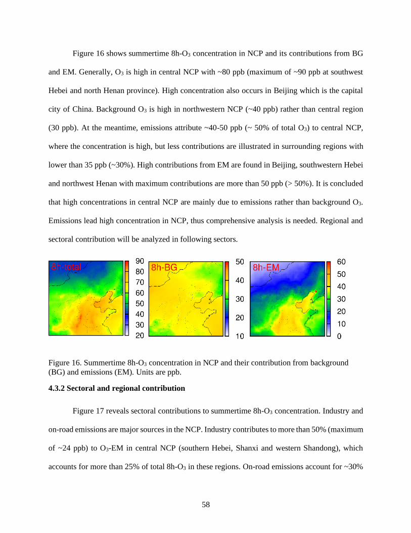
58
Figure 16 shows summertime 8h-O3 concentration in NCP and its contributions from BG
and EM. Generally, O3 is high in central NCP with ~80 ppb (maximum of ~90 ppb at southwest
Hebei and north Henan province). High concentration also occurs in Beijing which is the capital
city of China. Background O3 is high in northwestern NCP (~40 ppb) rather than central region
(30 ppb). At the meantime, emissions attribute ~40-50 ppb (~ 50% of total O3) to central NCP,
where the concentration is high, but less contributions are illustrated in surrounding regions with
lower than 35 ppb (~30%). High contributions from EM are found in Beijing, southwestern Hebei
and northwest Henan with maximum contributions are more than 50 ppb (> 50%). It is concluded
that high concentrations in central NCP are mainly due to emissions rather than background O3.
Emissions lead high concentration in NCP, thus comprehensive analysis is needed. Regional and
sectoral contribution will be analyzed in following sectors.
Figure 16. Summertime 8h-O3 concentration in NCP and their contribution from background
(BG) and emissions (EM). Units are ppb.
4.3.2 Sectoral and regional contribution
Figure 17 reveals sectoral contributions to summertime 8h-O3 concentration. Industry and
on-road emissions are major sources in the NCP. Industry contributes to more than 50% (maximum
of ~24 ppb) to O3-EM in central NCP (southern Hebei, Shanxi and western Shandong), which
accounts for more than 25% of total 8h-O3 in these regions. On-road emissions account for ~30%

59
of O3-EM in Beijing, Tianjin and central Hebei with maximum of ~50% (~10 ppb). High
contributions from energy sector are found at specific cities and regions in southern and
southwestern NCP by ~16 ppb, which accounts for maximum of 30% to total O3. Off-road
emissions contribute ~6 ppb to O3 along inland water channels in NCP and cause more than 10
ppb O3 above sea surface east to NCP. Residential, agriculture and biogenic emissions cause less
than 5 ppb in NCP, respectively. Wildfires also have low contributions except in south western
Hebei with maximum of ~5 ppb.
Figure 17. Summertime 8h-O3 contribution from sectoral emissions in NCP. Units are ppb.
Figure 18 reveals regional contributions to summertime 8h-O3 concentration. O3-EM is
generally affected by local emissions. For example, high concentrations in south Hebei, west
Shandong, Shanxi and north Henan are greatly dependent on local emissions (~70%) except O3
from background. Local emissions induce ~20 to 30 ppb O3 in high concentration region (with
maximum of ~35 ppb). It is noted that local emissions in Beijing and Tianjin provide maximum

60
of 20 ppb to local O3 formation, and they induce limited effects on each other (less than 5 ppb).
Due to being surrounded by Hebei, Beijing and Tianjin are affected by emissions from Hebei
significantly with 10% of total O3 from Hebei emissions (~10 ppb). Other provinces in NCP also
result in slightly effects on O3 formation in Beijing and Tianjin (less than 5 ppb). Local emissions
always result in 10 ppb O3 formation in conjunction area between neighbor provinces. At the
meantime, effects from long-distance transport are also observed. For instance, emissions in YRD
induce ~10 ppb O3 in whole southwestern Shandong and contribute to ~5 ppb O3 in southeastern
Hebei. Emissions from central China also affect O3 concentration in NCP by ~5 to 10 ppb.
Emissions from other regions (the rest provinces in China and other countries) have limited
impacts in NCP, but they affect O3 formation above ocean surface east to NCP by ~10 ppb.
Figure 18. Summertime 8h-O3 contribution from regional emissions in NCP. Units are ppb.

61
4.3.3 Source apportionment of O3 precursors
O3 contributions from total NOx and VOCs emissions are shown in Figure 19. Generally,
NOx accounts for more than 50% (maximum of ~80%) O3-EM in most provinces except Beijing
and Tianjin. NOx contributes to more than 25 ppb O3 formation in NCP, high contributions occur
in central NCP, which refers to south Hebei, north Henan and west Shandong with contributions
are evaluated to ~40 ppb. It is concluded that NOx is the major precursor in most NCP while
opposite phenomenon is observed at Shijiazhuang and southwestern Tianjin where VOCs
dominates O3 formation with more than 20 ppb while NOx induces ~10 ppb only. VOCs emissions
also dominate in specific cities such as Tianjin, Shijiazhuang, Baoding and Qingdao. VOCs
contributes less than 10 ppb to O3 in NOx dominant regions. O3 contributions from NOx and VOCs
emissions (by sectoral and regional groups) are detailed analysis from following discussions.
Figure 19. summer 8h-O3 contribution from NOx (8h-O3N) and VOCs (8h-O3V) in NCP. Units
are ppb.
Figure 20 shows regional contribution of summertime O3 from NOx and VOCs. Consisted
with previous discussion, local emissions (both NOx and VOCs) dominate local O3 formation. NOx
contributes more than 20 ppb to local O3 in high concentration regions such as south Hebei, north
Henan and west Shandong, which account for ~70% of total O3-EM in these regions. It is noted
that local NOx emissions also have significantly impacts to surrounding provinces and regions. For

62
example, NOx emissions from YRD induce ~5 to 10 ppb O3 in Shandong, which accounts for
approximately 20% of O3-EM. NOx dominant O3 formation lead high concentration in NCP for
most provinces except in Beijing and Tianjin. NOx accounts maximum of 40% O3-EM in Beijing
while NOx emission from Hebei accounts for 20%. VOCs emission affects less in most NCP
compared with NOx while VOCs also accounts for more than 30% of total 8h-O3 in specific regions
such as south Tianjin, Shijiazhuang, Tangshan, Taiyuan and Datong. Efforts from VOCs emissions
are much more significantly than NOx, thus VOCs dominates O3 formation in these regions.
Figure 20. Summertime NOx and VOCs regional contributions to 8h-O3 concentration. Units are
ppb.
Sectoral source apportionment results (Figure 21) reveal that O3 is mainly relied on NOx
emissions from all sources except biogenic emissions. Industry emissions induce maximum of ~20

63
ppb O3 formation related to NOx in central NCP. NOx emissions from energy sector also induce
~15 ppb in cities in south NCP. NOx emissions from on-road and off-road transportation form ~6
and ~9 ppb O3 in NCP, respectively. It is noted that they also form more than 10 ppb O3 above sea
surface east to NCP. VOCs emissions barely result in O3 formation (less than 2 ppb) for most
sources except the emission from industry and biogenic. VOCs emissions from industry cause 5
to 10 ppb O3 in specific cities such as Tianjin and Qingdao. High VOCs emissions from industry
and on-road transportation help to explain their contributions to O3 formation. Overall, NOx
emissions from industry, energy and on-road transportation contribute to greatly in NCP, they
provide ~75% of O3-EM, which account for ~40% of total O3 in NCP.

64
Figure 21. Summertime NOx and VOCs sectoral contributions to 8h-O3 concentration. Units are
ppb.
4.3.4 Comparison of 3R and other O3 regime schemes
O3 contributions from NOx and VOCs are calculated using different source analysis
techniques. In 3R scenario, NOx and VOCs related O3 formations in transition regime are classified
into O3N and O3V already, respectively. The concentrations and differences between each scenario
are shown in Figure 22. Basically, four source-oriented approaches predict same total O3
concentration in NCP, different attributions to NOx, VOCs and background compared with 3R are
shown. In first row, results from 3R indicate that high O3 concentrations are always occurred in
central NCP while north and northwest regions are under low concentration.

65
Figure 22. 8h-O3 contributions from NOx (O3N), VOCs (O3V) and background (O3-BG) in the
3R scenario (first row) and differences with 2R, NOx-limited and VOC-limited scenarios
(subtracting 3R by the results from each case). Units are ppb.
Due to O3 formations in NOx- and VOCs-limited cases only due to NOx and VOCs, thus
the differences with 3R are significant. O3V in VOCs-limited case is much higher (>20 ppb) than
in 3R widely in central NCP as well in surface of Bohai Sea. At the meantime, same situation

66
happens to NOx-limited case where O3 formation is due to NOx only, thus O3V is significantly
lower than in 3R. It is worthy to note that the differences between 3R and 2R provides interesting
findings. Generally, 3R predicts lower O3 contributions from NOx emission in NCP except in cities
such as Tianjin, Shijiazhuang and Taiyuan where more O3 formation (~6 ppb) are classified as to
from VOCs emissions. As results, 2R predicts more VOCs dominant cities than 3R, O3
contributions from VOCs are increased in these cities in 2R. Compared to single precursor limited
approaches, 3R predicts lower background O3 by ~ 5 ppb in central NCP. However, 2R has even
~3 ppb lower than 3R in these areas. Due to higher accurate O3 regime scheme that applied in
China, source apportionment results from this work indicate more contributions from NOx and less
from VOCs in major cities in NCP, these results help to better quantify impacts from emission
sources and for more accurate further analysis in O3-related impacts on human health, economic
benefits and ecosystem.
4.3.5 City scale analysis
Source apportionment analysis in major cities provide detailed evidences for controlling
strategies. Emissions and background contributions to total 8h-O3 in 8 NCP major cities are shown
in Table 11. Long-term urbanization and industrial development cause high contribution from
background O3 in NCP211, which accounts for ~50% of total O3 in these major cities. However, as
result of increasing emissions of O3 precursors (NOx and VOCs) 152, 212, O3 contributions from
emissions are nonnegligible. Emissions induce ~ 45% to 52% of total O3 in major cities except in
Datong where emissions only account for 35% of total O3. There are three peak episodes observed
in study period as discussed in chapter 2. O3 contributions from background O3 in these periods
are slightly higher while significant contributions from emissions are estimated as shown in Table
12. In all studied cities, high O3 concentrations are associated with emission sources which cause

67
more than 50% of total O3 formation (with maximum ~60% in Jinan and Taiyuan). It is concluded
that high pollution episodes are mainly due to emissions rather than background O3 contributions.
Sectoral source apportionment results (Figure 23) indicate industrial emission is the major source
of O3-EM, which results in more than 10 ppb O3 (more than ~33% of O3-EM, and maximum of
58% (Tianjin)). On-road and energy emissions also strongly affect O3 concentration. They account
for more than 70% (maximum of ~85%) O3-EM in major cities together with industrial emission.
Industry and on-road emissions account for ~65% of total O3 in Beijing as the results of high
population and emissions from mobile vehicles. It is noted that on-road emission has similar
attribution as industrial emissions in Beijing while it accounts significantly less in other major
cities. Energy emissions in Jinan has similar attribution as industrial emissions while on-road
emission has less impact on total O3-EM. Wildfires, agriculture, residential and biogenic emissions
are always having low impacts. Sectoral contributions in high concentration episodes reveal that
high O3 concentration in these periods are caused greatly from emission sources, which cause large
amount of O3 formation. More than 50 % of total O3 (more than 50 ppb) are estimated from
emission sources (as shown in right panel for each city in Figure 23). High emission contributions
are mainly caused from industry and energy emissions. In all major cities except Datong and
Baoding, contribution from industry emissions are increased by ~30 to 50% in high concentration
period, which refers to maximum of 10 ppb. Contributions from energy emissions are estimated
to more than twice in Baoding and Tangshan compared with regular summertime. It is also noted
that contribution from wildfire emissions also has obvious increase in Beijing.

68
Table 11. Summertime 8h-O3 contribution from background and emissions. Units are ppb.
8h-O3 Beijing Tianjin Shijiazhuang Baoding Tangshan Jinan Datong Taiyuan
Total 73.04 71.89 72.80 74.96 68.8 77.63 60.93 72.18
BG 37.54 38.21 38.69 37.52 37.27 36.53 39.27 38.87
EM 35.5 33.68 34.11 37.44 31.53 40.90 21.66 33.31
• EM: O3 contribution from emissions; BG: contribution from background
Table 12. 8h-O3 concentration and its contribution from background and emissions in peak episodes. Units are ppb.
8h-O3 Beijing Tianjin Shijiazhuang Baoding Tangshan Jinan Datong Taiyuan
Total 96.55 94.24 93.59 94.01 95.57 91.92 66.3 98.05
BG 41.54 42.48 41.72 41.56 40.22 37.19 39.8 40.24
EM 55.01 51.76 51.87 52.45 55.35 54.73 26.5 57.81
• EM: O3 contribution from emissions; BG: contribution from background

69
Figure 23. 8h-O3 contributions from sectoral emissions in major city in summertime (left
column) and peak episodes (right column). Units are ppb.
Regional source apportionment (Figure 24) reveals the similar results as other studies that
local emission would be the major source of O3-EM. However, impacts from surrounding regions
are also nonnegligible. For example, local emission in Beijing accounts for 50% of O3-EM while
emissions from Hebei also induce ~20% of them. Being Surrounded by Hebei makes Beijing very
sensitive to emissions from Hebei. However, Tianjin has different situation even if it is also
surrounded by Beijing and Hebei. O3-EM in Tianjin are mainly due to local emissions but less to
emissions from surrounding regions. It might be because the geophysical characters in Tianjin that
emissions from Hebei and Beijing will be limited locally or spread to ocean surface southeast to
Tianjin. Further analysis in needed in future for this. Emissions from north and central China also
has slight impacts on O3-EM in NCP with ~2-6 ppb. Analysis of regional source apportionment
indicates an interesting finding. Though contributions from local emission increased, emissions
from central China have strong impacts on increasing O3 concentration in central, south and
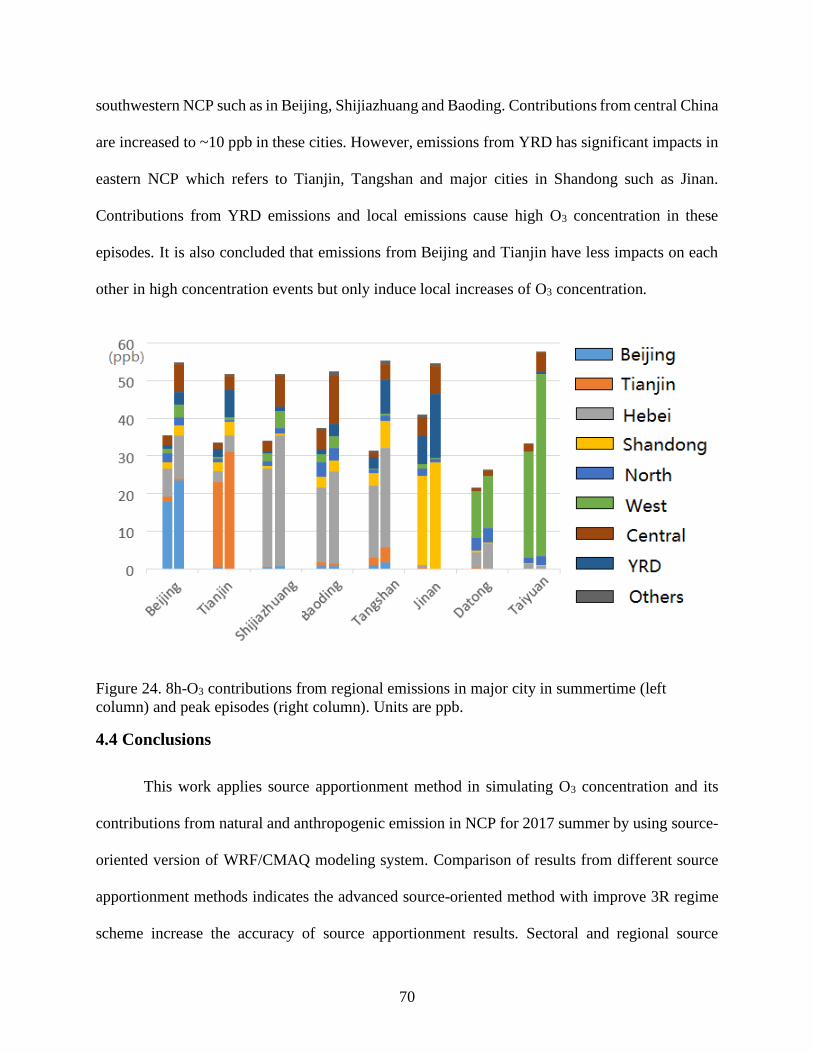
70
southwestern NCP such as in Beijing, Shijiazhuang and Baoding. Contributions from central China
are increased to ~10 ppb in these cities. However, emissions from YRD has significant impacts in
eastern NCP which refers to Tianjin, Tangshan and major cities in Shandong such as Jinan.
Contributions from YRD emissions and local emissions cause high O3 concentration in these
episodes. It is also concluded that emissions from Beijing and Tianjin have less impacts on each
other in high concentration events but only induce local increases of O3 concentration.
Figure 24. 8h-O3 contributions from regional emissions in major city in summertime (left
column) and peak episodes (right column). Units are ppb.
4.4 Conclusions
This work applies source apportionment method in simulating O3 concentration and its
contributions from natural and anthropogenic emission in NCP for 2017 summer by using source-
oriented version of WRF/CMAQ modeling system. Comparison of results from different source
apportionment methods indicates the advanced source-oriented method with improve 3R regime
scheme increase the accuracy of source apportionment results. Sectoral and regional source

71
apportionment analysis indicate that industry, energy and on-road emissions are the major sources.
Contributions from on-road and industry are significantly increased in peak episodes. Local
emissions and emissions from surrounding regions are main sources of O3 formation. Emissions
from central China have significant impacts in Beijing, central, south and southwestern NCP while
Tianjin, eastern NCP are more associated with emissions from local and YRD. This work provides
information for estimating regional and sectoral contributions to O3 pollution, which helps to
deeper understand the sources of high O3 concentration. It also offers solid evidences for further
estimation of health risk. An effective emission controlling strategies can be designed based on
results of this work to reduce O3 concentration in future.

72
CHAPTER 5. OZONE SOURCE APPORTIONMENT IN
SOUTHEAST U.S.
5.1 Introduction
O3 is a secondary pollutant which is associated with a long-standing air quality problem in
the U.S. for decades. Though O3 concentration has significantly decreased through efforts from
reducing anthropogenic emissions, many nonattainment events are observed over the U.S., and the
O3 concentration has remained higher than NAAQS requested threshold of 70 ppb in some regions
213 26, 55, 214. Many studies analyzed O3 variation trends and impact factors in high concentration
area over the U.S. A springtime increases of O3 concentration were reported in western U.S. rural
area by 0.2-0.5 ppb, while the increases were recorded in wintertime over eastern U.S.215. Dry
deposition was revealed as the primary sink for O3 and it was estimated to be increased in
southeastern U.S.216. The increased air stagnation also induced significantly positive effect to raise
O3 concentration associated with dry tropical weather in midwestern U.S.217. Global warming trend
was proved to induce high O3 concentration events in mid-Atlantic region of the U.S. under a 30-
years historical analysis218.
Increasing concern of O3 pollution requires researcher to analyze sources of O3 formation.
Background O3 concentration was estimated to shift maximum O3 event to early summer, and its
contribution from global anthropogenic emission was estimated to be increased over the past
decades especially in western U.S.26, 219. Decreases of emission of NOx and VOCs cause a
reduction of averaged ambient O3 concentration by ~22% since 1998 220. BVOC emission was
reported as the major source of VOCs emission in the U.S., which accounted for 75% to 80% of
total VOCs emissions. BVOC was classified as a significant contributor to regional O3

73
concentration in SUS118, 221. In peak episodes, reductions of NOx emissions from mobile vehicles
and point source were estimated to cause the largest reductions O3 concentration in Texas, U.S.222.
O3 formation is very sensitive to emissions of precursors, thus many approaches were
applied to quantify the O3 source contributions from NOx and VOCs. BVOC was estimated as the
major precursor of O3 formation for extreme O3 events in SUS223. But contributions from other
sources are not well studied. This work aims to quantify O3 sensitivity to precursors and
contribution from all emission sources, which will provide information to estimate health impacts,
economic benefits and further emission controlling strategies to reduce O3 concentration so that to
match NAAQS requested threshold.
5.2 Methods
5.2.1 Model description
O3 concentration and its contributions from emission sources are simulated by applying the
CMAQ model (version of 5.0.1) with SAPRC99 photochemical mechanism and AERO6 aerosol
chemistry179, 207. Meteorological conditions are generated by the Weather Research and
Forecasting (WRF) version of 3.7.1 with initial condition (ICs) and boundary conditions (BCs)
from WRF preprocessing system (WPS), which is obtained from FNL operational global analysis
data from National Center for Atmospheric Research (NCAR,
http://dss.ucar.edu/datasets/ds083.2/). Emission Database of Gas and Atmospheric Research
(EDGAR) provides anthropogenic emission of 2012 and they are scaled to 2016 based on EPA
National Emission Inventory (NEI) Technical Support Document (TSD)
(https://www.epa.gov/air-emissions-inventories/2014-national-emissions-inventory-nei-
technical-support-document-tsd) which includes variation trends of NOx and VOCs emissions for
each sector from 2012 by state scale. Scale factors for NOx and VOCs emissions in SUS are list in

74
Figure 14 and Figure 15. Biogenic emissions for 2016 are provided by the Model for emissions of
Gases and Aerosols from Nature (MEGAN) 184, and Fire Inventory from NCAR (FINN) 185 is used
to generate open-burning (wildfires) emissions for simulation period. O3 source-oriented method
is applied in tracking O3 contribution from emission sources by tagging reactive NOx and VOCs
tracers as descripted in chapter 3134, 208, 209. Benefits Mapping and Analysis Program (BenMAP)
model helps to analyzes health impacts associated with O3 by applying functions recruited from
the published epidemiology literature. These functions calculate health impacts by used value of
pollutant concentrations, population, incidence baseline rates and coefficients for different health
endpoints, which are from simulation results (pollutant concentration) and BenMAP database,
respectively, in every grid in study domain.
Table 13. Scaling factor for NOx emissions for major states in SUS.
LA AR MI TN AL GA FL NC SC
Energy 0.77 0.83 0.45 0.70 0.45 0.46 0.71 0.73 0.42
Industry 0.74 1.23 1.02 0.91 1.11 0.98 0.81 0.89 0.85
Residential 0.83 1.79 1.07 1.13 0.68 1.09 1.14 1.11 1.15
Agriculture 0.91 1.03 0.86 1.25 1.19 1.04 1.23 1.11 1.14
On-road 0.83 0.74 0.54 0.69 0.73 0.72 0.72 0.67 0.70
Off-road 0.43 0.84 1.19 0.78 0.98 0.77 0.94 0.82 0.97
Table 14. Scaling factor for VOCs emissions for major states in SUS
LA AR MI TN AL GA FL NC SC
Energy 0.86 0.97 0.92 0.98 1.17 0.96 0.96 0.94 0.80
Industry 0.98 1.22 0.89 0.81 0.82 1.21 0.94 1.11 0.89
Residential 1.38 1.03 0.48 1.29 1.60 1.74 0.98 1.48 1.46
Agriculture 1.07 1.12 1.20 1.20 1.09 1.06 0.91 1.15 1.06
On-road 0.68 0.79 0.62 0.72 0.75 0.73 0.68 0.64 0.79
Off-road 0.74 0.81 0.85 0.79 0.82 0.78 0.75 0.78 0.78
.

75
5.2.2 Model application
O3 and its source apportionment are simulated in a coarse domain with resolution of 36km
covering the U.S. except Alaska and Hawaii. Part of surrounding countries such Canada and
Mexico are also included. Nested finer domain covers SUS with resolution of 12km. Finer domain
includes Alabama (AL), Arkansas (AR), Florida (FL), Georgia (GA), Louisiana (LA), Mississippi
(MI), North Carolina (NC), South Carolina (SC) and Tennessee (TN) and part of neighbor states.
Domain settings are shown in Figure 25. Emissions from agriculture, energy, industry, on-road,
off-road, residential, biogenic and wildfires are tracked by tagging NOx and VOCs species in
emissions inputs. Meteorological and emission inputs for June are generated used to predict
summertime O3 behavior in both domains. Three regime scheme (3R) is applied as O3 sensitivity
chemical scheme to precursors of NOx and VOCs as described in previous chapter53.

76
Figure 25. Domain setting of SUS. Outer domain represents parent domain (36km by 36km)
covered the United State except Alaska, Hawaii etc. Nested 12km by 12km domain (d02) cover
SUS in this study.
5.3 Results and discussions
5.3.1 Overall O3 simulations
Summertime 8h-O3 concentrations in U.S. are simulated and shown in
Figure 26, its contributions from background and emission sources are also illustrated.
High concentrations occur in western, southwestern and northeastern U.S. with averaged
concentration of more than 50 ppb. Highest pollution event is observed in southwest California by
concentration of more than 70 ppb. Background O3 is the major source in western U.S., which
provides O3 formation ranged from 40 to 50 ppb in most west regions. However, contribution from
background O3 is decreased in central and eastern U.S., corresponds to ~30 ppb. Minimum

77
contribution is observed in SUS with less than 25 ppb. Emissions play essential roles in forming
O3 in coastal California and low background contribution area such as central and eastern regions.
Maximum contributions are predicted in southwest California and coastal northeastern U.S. by
more than 30 ppb. High contribution also occurs around Lake Michigan and Kentucky by ~20 to
30 ppb.
Figure 26. Summertime 8h-O3 concentration in U.S. and its contribution from background (BG)
and emissions (EM). Units are ppb.
Model performance of O3 predictions in SUS are validated following same suggested
statistic criteria 200 introduced in Chapter 2. Predicted O3 concentrations are compared with
observation data recorded from a total of 224 monitoring stations in SUS. The statistic results are
shown in Table 15. The MFE in all states match well with suggested benchmark of 0.35, but
slightly exceedances of MFB are found in GA, NC, SC and TN. The NMB in these regions also
exceed suggested criteria. Biases in these states are mainly due to uncertainties in domain edging
area. Model slightly overestimates concentrations in SUS, biases are less than 2 ppb in FL, LA and
MI, the best performance is found in LA with bias less than 1 ppb. However, model has a
significantly overpredictions in part of central and north SUS such as in NC and TN with
exceedances of both MFB and NMB. Biases are mainly due to uncertainties from emissions
inventories and model resolutions224, 225. Overall, 8h-O3 predictions in SUS agree well with
observation from a total of 244 monitoring stations in SUS. Results from this simulation are
reliable for further analysis. Overall, O3 concentrations in SUS (Figure 27) are less than 50 ppb

78
except north and west regions. A decrease trend is found from inner land to coastal area. However,
contribution from background is high in the northeastern Gulf of Mexico and coastal Florida and
Georgia by ~35-40 ppb but low in inland SUS where ~25-30 ppb O3 formations are estimated due
to background O3. It is noted that emissions strongly affect O3 formation in central and northwest
SUS. Detailed analysis is conducted in following section.
Table 15. Model performances in 9 states in SUS for 8h-O3 simulation. Units are ppb for OBS
and PRE. Bold represents the statistical result exceeds criteria.
AL AR FL GA LA MI NC SC TN Benchmark
OBS 39.13 41.88 36.45 41.31 39.05 41.00 44.39 41.18 43.58
PRE 45.31 46.93 37.03 50.20 39.24 42.81 53.20 50.40 53.58
MFB 0.12 0.10 -0.01 0.17 -0.03 0.02 0.17 0.19 0.20 ±0.15
MFE 0.25 0.23 0.28 0.29 0.29 0.23 0.25 0.27 0.27 0.35
NMB 0.18 0.15 0.04 0.24 0.02 0.07 0.22 0.26 0.27 ±0.15
Figure 27. Summertime 8h-O3 concentration in SUS and its contribution from background (BG)
and emissions (EM). Units are ppm.
5.3.2 Source apportionment in SUS
Figure 28 indicates that emissions from NOx dominate O3 formation in SUS and barely
O3 contributions are estimated from VOCs. NOx emissions have strong impacts in northwest
SUS, they cause more than 20 ppb O3 formation in this region. Their impacts are significantly
reduced from northwest to southeast regions, and they cause less than 10 ppb O3 in south SUS

79
and even less than 5 ppb in south Florida. Impacts from VOCs emissions are generally lower
than 2 ppb except in specific cities such as in Houston, Dallas and Nashville where ~5 ppb O3
are estimated to associate with VOCs emissions.
Figure 28. 8h-O3 contributions from emissions of NOx and VOCs. Units are ppb.
Sectoral contributions are shown in Figure 29. More than 10 ppb O3 are from on-road
emissions in north SUS, and contributions from on-road emissions are decreased to ~3 ppb in
central and south regions. Emissions from energy mainly induce O3 increasing in north and west
SUS by 6 to 8 ppb but cause less impacts on central and southeast regions with less than 2 ppb.
Industry has slightly lower contribution than energy emissions, it causes ~4 to 6 ppb O3 in specific
cities in central and west SUS. Besides, significant contributions from biogenic emissions are
found in west and northwest SUS, around 4 ppb O3 are estimated from biogenic sources. It is
concluded that on-road emissions are the major sources in SUS followed by emissions from energy,
industry and biogenic sector. On-road and biogenic emissions prefer to induce O3 concentration in
north and northwest area while emissions from energy and industry have strong impacts on specific
cities in north and west SUS.

80
Figure 29. 8h-O3 contributions from emission sectors. Units are ppb.
Since O3-EM in SUS is mainly dominated by NOx, a deeper analysis of its source
apportionment would carry out a comprehensive understanding. 8h-O3 contribution from emission
sources for NOx and VOCs are illustrated in Figure 30. It is noted that VOCs emissions has barely
impacts on O3 formation except the emissions from biogenic and industry. Biogenic emissions are
the major sources of VOCs-related O3, which cause significant impacts in northwestern regions.
VOCs industry emissions cause ~ 1 ppb O3 formation in Houston, Dallas and Atlanta, their impacts
on other SUS regions are less than 0.5 ppb. Contributions from NOx emission has similar spatial
pattern as total source contributions, which means a leading position of on-road emissions
followed by energy emissions.

81
Figure 30. Summertime NOx and VOCs contributions to 8h-O3 by sectors. Units are ppb.
5.3.3 Comparison with China
From the results of previous chapters, anthropogenic emissions induce higher contributions
in NCP, which lead average of ~30 ppb O3 in summertime and maximum of more than 50 ppb in
peak episodes. However, both anthropogenic emissions of NOx and VOCs are significantly lower
in SUS than in NCP. As shown in
Figure 31, summertime monthly average total NOx emissions are ~10-20 tons in SUS with
maximum of more than 200 tons in megacities such as Houston, Dallas and Atlanta. NOx emissions
are generally higher than 100 tons in central NCP with maximum of more than 300 in specific city
such as Beijing, Tianjin and Shijiazhuang. VOCs emissions in NCP also significantly higher than
SUS.

82
Figure 31. Summertime average monthly emissions of NOx and VOCs and contribution from
anthropogenic sources in SUS. Units are tons/month.
Both NCP and SUS has high energy NOx emissions but emissions from other sectors are
extremely lower in SUS especially for on-road, off-road and energy emissions which are major
sources in NCP. High emissions only occur in specific cities in SUS such as Houston, Dallas and
Atlanta while emissions in NCP are generally high in most central regions. It is noted that overall
NOx emissions are at the low level (by ~10-20 tons/month) in SUS while a decrease trend is found
in NCP from south to north (from 50 tons/month to less than 10 tons/month). VOCs emissions
from anthropogenic sources are all significantly lower in SUS with a maximum of ~8 tons/month
while the high VOCs emissions in NCP are more than 10 tons/month. As the major VOCs
contributors in SUS, emissions from on-road and industry are lower than half of them in NCP.
Generally, NOx and VOCs emissions in SUS are at low levels with only specific high emissions
in major cities in each state, and even the high emissions in these cities are much lower than in

83
most regions in NCP. Emissions in NCP are generally higher in south and central regions. O3 is
estimated to sensitive to emissions in both NCP and SUS, differences in emissions cause greatly
impacts on O3 formation, thus O3 source apportionment analysis in these regions helps to
understand different source contributions under various emission conditions.
Major anthropogenic emission sources are industry, energy and on-road which occupied
more than 70% of total O3-EM in NCP while on-road emissions are the only major anthropogenic
source in SUS, less contributions from industry and energy sectors are estimated. Compared to
anthropogenic emissions, biogenic emissions contribute less in NCP by causing less than 3 ppb O3
while it becomes one of the major sources in SUS followed by on-road and energy emission. The
maximum contribution from biogenic emissions of more than 5 ppb is occurred in western SUS.
Contributions from emission sources show different patterns in NCP and SUS, which request an
emergent requirement of reducing emissions from industry and energy so that the O3 pollution
could be reduced to matching its level in SUS.
5.4 Conclusions
This work simulates summertime O3 concentration in SUS and its contributions from
anthropogenic and natural emission sources. Model performances are validated. Though
overestimations are remained in northern SUS, simulation results are generally match agree well
with observation data and reliable for further analysis. High concentrations are found in north and
west regions with the concentration of 8h-O3 higher than 40 ppb. A decrease trend is found from
northwest to southeastern coastal regions. Background O3 contributes ~25 to 30 ppb in SUS while
emission sources have strong impacts in high concentration regions by inducing ~30 ppb O3
formation. O3 formation in SUS is mainly dominated by NOx while VOCs emissions cause
maximum of 5 ppb in Houston, Dallas and Nashville. Major contributors of NOx-related O3

84
formation are on-road emissions followed by energy, industry and biogenic emissions while
biogenic emissions are major sources of O3V. Comparison between SUS and NCP carries out that
anthropogenic emissions cause the high O3 pollution in NCP. Major sources in NCP are industry,
energy and on-road emissions while on-road emission is the only major source in SUS. Results of
this work provide information for further estimation of health risk analysis and offer solid evidence
for designing the controlling strategies to reduce O3 concentration in NCP.

85
CHAPTER 6. OZONE ASSOCIATED HEALTH RISK ANALYSIS
6.1 Introduction
Ground-level O3, which was listed as one of six major air pollutants as set in NAAQS by
EPA, is a highly toxic gas that have harmful effects on human health213, 226, 227. Inhaling O3 causes
irritation, inflammation and constriction to human respiratory system and results in health impacts
such as decreases of breathing functions, asthma attacks, hearth attacks and premature mortality
228, 229. Around 142 thousand premature mortalities were estimated with O3-related COPD caused
by long-term O3 exposure globally229. A total of 9-23 million annul asthma emergency room visits
were also reported correspond to O3 pollution around the world. At the meantime, China is shown
as one of the most polluted countries that largest impacts from O3-related health issues were
estimated 230.
China is experiencing O3 increases issue, a total of 318 cities were revealed to exceed WHO
recommended O3 concentration, and 69 of them failed to meet the NAAQS target of China231.
Many studies tried to quantify O3 impacts on human health in China. A total of 816.04 million
cumulative population was estimated exposed to a circumstance that 8h-O3 concentration is higher
than 100 µg/m3 in China, which results in around 55 to 80 thousand premature mortality caused
by COPD in 2015. At the meanwhile, Beijing, Shandong, YRD, PRD and Sichuan basin were
listed as high risk region14. A growth rate of mortality increased from 0.42% to 1.11% around
China as the result of O3-related health issue were estimated, which corresponded to 28 to 74
thousand premature mortality232. O3-related health risk is also detailed analyzed in high O3 risk
area. A 39.5% (1100 deaths) increased of premature mortality was estimated as result of O3

86
pollution in PRD233. An increase of 10 μg/m3 of 8h-O3 were associated with 0.55% increases of
total mortality in Jiangsu Province. Increases of mortality due to hypertension, coronary diseases
and stroke were revealed to associate with 10 μg/m3 increases of 8h-O3 country wide by 0.60%,
0.24% and 0.29%, respectively234. It was reported that more than 3 million respiratory symptoms
and 1 million cases of school-loss days would be avoided if O3 concentration could be controlled
to lower than 75 ppb in the U.S.235. Around 0.11% to 0.27% increases of O3-related daily mortality
were revealed on average across 50 cities in U.S., which were associated with increases of daily
1h-O3 by average of 4.8 ppb (maximum of 9.6 ppb) 236.
O3 exposure leads a series of adverse health effects including premature mortalities of
respiratory and cardiovascular diseases237, 238. The concentration response function (CRF) is
widely used in WHO and previous studies to quantify O3-related health impacts239, 240. The change
rates of 0.42%, 0.44% and 0.50% of mortality due to non-accidental causes, cardiovascular
diseases and respiratory diseases were estimated as the result of an increased 8h-O3 concentration
of 10 µg/m3, respectively241. Increase of 10 µg/m3 of daily averaged O3 concentration was also
estimated to cause increase of 0.6% nonaccidental mortality in China231. However, there is no
study detailed provides O3-related health impacts in NCP and their contribution from emission
sources. Studies in U.S. is also limited in analyzing health impacts from emission sources. This
study will recruit results from previous chapters and apply the reliable health analysis methods to
estimate O3-related health risk in NCP and SUS as well as source contribution in these regions.
Results of this study provides information to assess health risk caused by human activities and
quantify the contributions from emissions sources. Health analysis results would be further used
to estimation on economic benefits.

87
6.2 Methods
China-specific concentration-response functions (CRF) 242, 243 are adapted in this study to
estimate the health impacts due to exposure of O3. Cardiovascular and respiratory mortalities are
calculated in this study. Relative risk (RR) of Cardiovascular and respiratory disease mortalities
with a 95% confidence interval with corresponding 8h-O3 concentrations are calculated using
following equation:
Equation 18:
𝑅𝑅𝑖 = exp [𝛾(𝐶𝑖 − 𝐶0)]
Where i refers to the index of the domain grid. 𝛾 is fitted by meta-regression based on the
previous epidemiological studies for China 242. Ci and C0 are the pollution concentration in the
target grid and the threshold value, below which will induce no additional risk, respectively.
Threshold concentration of 8h-O3 is 35 ppb (equivalent to 70 μg/m3) in this work172. Extra health
impacts are resulted from concentration higher than the threshold value. The health endpoints (E)
for CRF is calculated based on following equation:
Equation 19:
𝐸 =∑𝑅𝑅𝑖 − 1
𝑅𝑅𝑖∗ 𝑃𝑖 ∗ 𝐹𝑖
𝑖
Where Pi and Fi refer to population and baseline incidence rate. It is noted that health
endpoints in this study include premature mortality due to respiratory diseases (RDM) and
cardiovascular diseases (CDM). Major respiratory and cardiovascular diseases including chronic
obstructive pulmonary disease (COPD) , ischemic heart disease (IHD) and strokes (STK, including
both ischemic and hemorrhagic strokes) are also calculated in this analysis. The baseline incidence
rates are obtained from the online GBD database (http://vizhub.healthdata.org/gbd-compare/). The

88
United Nations (UN)-adjusted population distribution for year of 2017 from the Center for
International Earth Science Information Network (CIESIN) is used to represent the population
exposure.
CRF is a long-term concentration related function, thus simulated summertime 8h-O3
concentrations are scaled to annual concentrations by applying provincial average ratio calculated
from observation data recorded in monitoring stations following Equation 20 for each grid.
Equation 20:
𝐴𝑛𝑛𝑢𝑎𝑙 8ℎ˗𝑂3(𝑆) = 𝑆𝑢𝑚𝑚𝑒𝑟 8ℎ˗𝑂3 (𝑆) ×𝐴𝑛𝑛𝑢𝑎𝑙 8ℎ˗𝑂3 (𝑂)
𝑆𝑢𝑚𝑚𝑒𝑟 8ℎ˗𝑂3 (𝑂)
S and O in equation (3) refer to concentration from simulation and observation,
respectively. Observation data are provided by China National Environmental Monitoring Center
(CNEMC, http: //113.108.142.147:20035/emcpublish/).
Benefits Mapping and Analysis Program (BenMAP) model helps to estimate the O3-related
health risk in SUS. Health endpoints includes mortality (all-cause, respiratory and
cardiopulmonary diseases), emergency room (ER) visits (for asthma) and hospital admissions (HA,
for all respiratory). Health impacts are calculated by applying recruited function from published
epidemiology literature in this model. Health impacts are associated with pollution concentrations,
population and incidence baseline rates, which are from results of previous chapters and BenMAP
database in U.S.

89
6.3 Results and discussions
6.3.1 Overall health risk in NCP
Based on discussions in previous chapters, simulation results for O3 concentrations in NCP
are in sufficient agreement with observations to act as basis for health impacts analysis. It is noted
that annual 8h-O3 concentrations are scaled from summertime concentration in this estimation.
Health risks are estimated for both MEIC and EDGAR+ simulation results. Health impacts in
Beijing, Tianjin, Hebei, Shandong and Shanxi are included in the following discussion while the
rest provinces are not included since they are not fully contained in the simulation domain. Results
from MEIC and EDGAR+ are listed in Table 16. Due to the higher predicted concentration, MEIC
results in a higher risk for all health endpoints. MEIC predicts a total of 0.13 million mortalities
for all causes (0.05 million for RDM and 0.08 million for CDM) while EDGAR+ predicts ~0.02
million fewer mortalities than MEIC (total of 0.04 and 0.07 million for RDM and CDM,
respectively). COPD is the major disease within RDM, accounting for around 1/3 of total mortality
in simulations. Both EDGAR+ and MEIC predict similar relative health impacts in different
provinces. Hebei and Shandong have the highest impacts with more than total of 0.04 million
mortalities. Shanxi also has high mortality followed by Beijing and Tianjin. With high population,
Beijing and Tianjin also have severe health problems under high O3 concentration. Beijing has
~0.01 million all-cause mortality, which is twice as high as in Tianjin.
Table 16. Provincial health risk analysis results within the NCP. Units for health endpoints are
cases.
Beijing Tianjin Hebei Shandong Shanxi Total
Total
mortality
EDGAR+ 9536 4809 40902 40840 16302 112390
MEIC 12062 5395 45460 48602 19022 130541
(Table cont’d)

90
1. Cardiovascular diseases mortality (CDM); respiratory diseases mortality (RDM); ischemic heart disease
(IHD); stroke (STK); chronic obstructive pulmonary disease (COPD).
2. Only Beijing, Tianjin, Hebei, Shandong, Shanxi are completely included in this study, the health result
for the rest provinces (Rest) are only refer to the part that included in this study domain.
3. Total mortality includes CDM and RDM only.
Due to higher accuracy of concentration results using EDGAR+, spatial distributions of
mortality from each disease in EDGAR+ results are shown in Figure 32. The differences between
EDGAR+ and MEIC are also shown in Figure 33. Health endpoints in major cities/provinces are
also listed in
Beijing Tianjin Hebei Shandong Shanxi Total
CDM EDGAR+ 5884 2975 25276 25341 10130 69606
MEIC 7389 3324 27991 29964 11750 80418
RDM EDGAR+ 3652 1834 15626 15499 6172 42783
MEIC 4673 2071 17469 18638 7272 50123
COPD EDGAR+ 3582 1798 15325 15200 6054 41959
MEIC 4583 2031 17132 18279 7132 49157
IHD EDGAR+ 2796 1614 12011 12042 4814 33277
MEIC 3511 1580 13301 14239 5583 38214
STK EDGAR+ 2745 1388 11792 11822 4726 32473
MEIC 3447 1551 13058 13978 5481 37515

91
Table 17. Due to the higher predicted concentration, MEIC results in a higher risk for all
health endpoints. MEIC predicts a total of 0.13 million mortalities for all causes (0.05 million for
RDM and 0.08 million for CDM) while EDGAR+ predicts ~0.02 million fewer mortalities than
MEIC (total of 0.04 and 0.07 million for RDM and CDM, respectively). COPD is the major disease
within RDM, accounting for around 1/3 of total mortality in simulations. The spatial pattern
indicates that adverse impacts usually peak at megacities in the central NCP such as Beijing,
Tianjin and Shijiazhuang. Although O3 concentrations are not always extremely high in Beijing,
high population density leads to this serious health impacts. Such situations are also observed in
capital cities in other provinces such as Zhengzhou, Shijiazhuang as well as some big cities with
large population such as Tianjin and Yantai. In north Henan and south Hebei, severe health impacts
are also estimated due to the high O3 concentration instead of high population density. However,
opposite to central NCP, adverse health impacts are not very serious in coastal regions where O3
concentrations are relatively lower compared to central NCP except in specific high population
cities. In north, west and northwest NCP, O3-related health impacts are very low due to both low
O3 concentration and population. Figure 33 reveals that EDGAR+ predicts lower health risk than
MEIC except in specific cities such as Tangshan, Shijiazhuang, Qingdao and Taiyuan by 10~20
cases/grid. It is significant that EDGAR+ predicts lower mortality (20 cases/grid) in Beijing, where
EDGAR+ has higher accuracy in predicting O3. It is believed that EDGAR+ also predicts health
risk more accurately than MEIC.

92
Table 17. Provincial health risk analysis results within the NCP. Units for health endpoints
are cases.
1. Cardiovascular diseases mortality (CDM); respiratory diseases mortality (RDM); ischemic heart disease (IHD); stroke (STK); chronic obstructive pulmonary disease (COPD).
2. Only Beijing, Tianjin, Hebei, Shandong, Shanxi are completely included in this study, the health result
for the rest provinces (Rest) are only refer to the part that included in this study domain.
3. Total mortality includes CDM and RDM only.
Province Beijing Tianjin Hebei Shandong Shanxi Total
Total
mortality
EDGAR+ 9536 4809 40902 40840 16302 112390
MEIC 12062 5395 45460 48602 19022 130541
CDM EDGAR+ 5884 2975 25276 25341 10130 69606
MEIC 7389 3324 27991 29964 11750 80418
RDM EDGAR+ 3652 1834 15626 15499 6172 42783
MEIC 4673 2071 17469 18638 7272 50123
COPD EDGAR+ 3582 1798 15325 15200 6054 41959
MEIC 4583 2031 17132 18279 7132 49157
IHD EDGAR+ 2796 1614 12011 12042 4814 33277
MEIC 3511 1580 13301 14239 5583 38214
STK EDGAR+ 2745 1388 11792 11822 4726 32473
MEIC 3447 1551 13058 13978 5481 37515

93
Figure 32. Health end point results of five O3-associated diseases. Total shows the total
mortality due to O3-related diseases including RDM, CDM COPD, IHD and STK. Units
are cases/grid.

94
Figure 33. Difference of health endpoints between EDGAR+ and MEIC (subtracting
EDGAR+ by MEIC). Units are cases/grid.
Health outcomes from EDGAR+ and MEIC are compared with others’ studies for China
as shown in Table 18. Most studies used similar function (CRF) to estimate health risk with
different corresponding concentrations and thresholds. Mostly, 8h-O3 is used as the concentration
metric in the CRF with a threshold of 75.2 μg/m3. This study uses a slightly lower threshold (70
μg/m3) which is validated and successfully used in previous works 172, 235. Though the national
health impacts from other studies are calculated for different years by using varied thresholds, this
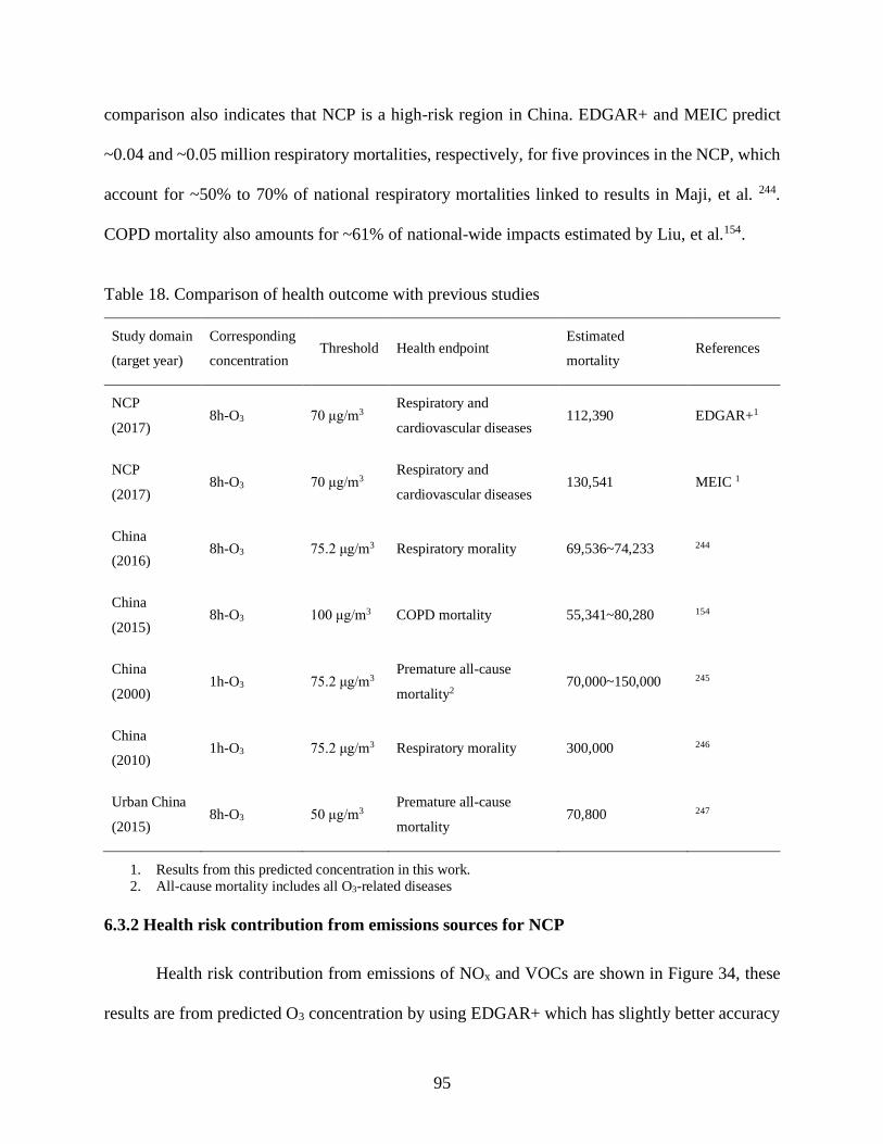
95
comparison also indicates that NCP is a high-risk region in China. EDGAR+ and MEIC predict
~0.04 and ~0.05 million respiratory mortalities, respectively, for five provinces in the NCP, which
account for ~50% to 70% of national respiratory mortalities linked to results in Maji, et al. 244.
COPD mortality also amounts for ~61% of national-wide impacts estimated by Liu, et al.154.
Table 18. Comparison of health outcome with previous studies
Study domain
(target year)
Corresponding
concentration Threshold Health endpoint
Estimated
mortality References
NCP
(2017) 8h-O3 70 μg/m3
Respiratory and
cardiovascular diseases 112,390 EDGAR+1
NCP
(2017) 8h-O3 70 μg/m3
Respiratory and
cardiovascular diseases 130,541 MEIC 1
China
(2016) 8h-O3 75.2 μg/m3 Respiratory morality 69,536~74,233 244
China
(2015) 8h-O3 100 μg/m3 COPD mortality 55,341~80,280 154
China
(2000) 1h-O3 75.2 μg/m3
Premature all-cause
mortality2 70,000~150,000 245
China
(2010) 1h-O3 75.2 μg/m3 Respiratory morality 300,000 246
Urban China
(2015) 8h-O3 50 μg/m3
Premature all-cause
mortality 70,800 247
1. Results from this predicted concentration in this work.
2. All-cause mortality includes all O3-related diseases
6.3.2 Health risk contribution from emissions sources for NCP
Health risk contribution from emissions of NOx and VOCs are shown in Figure 34, these
results are from predicted O3 concentration by using EDGAR+ which has slightly better accuracy

96
in matching averaged O3 concentration in NCP. Emission-related O3 causes ~46.5% of total
premature mortality while the rest of them are due to background O3 (53.5%). It is noted that NOx
is the major source in NCP while both NOx and VOCs have great impacts on megacities such as
Beijing, Tianjin and Shijiazhuang where have high level of both population and O3 pollution. For
major cities/provinces in NCP, total of 52,346 premature mortalities are estimated due to emissions.
NOx emissions cause 82.5% of emission-related premature mortality, correspond to 43,211 deaths.
Hebei and Shandong provinces have highest premature mortality, a total of 19.16 and 19.02
thousand deaths are estimated due to emissions, a total of 5 thousand mortalities are estimated for
Beijing. Source contributions to mortality are shown in Figure 35, which is associated with
concentration distribution. Industry, energy and on-road emissions are major sources that cause
79% of the total emission-related mortality. Emissions from Central China, Hebei and Shandong
provinces are the major sources of O3-related premature mortality, they cause a total of 55%
emission-related premature mortality. Spatial distribution of regional and sectoral emissions
contributions (Figure 36) indicates that local emissions are the major health issue sources, and
emissions in Hebei, Shandong and central China cause high health risk to central NCP, they cause
large amount mortality in central NCP. At the meantime, high contributions from emissions from
Beijing and Tianjin are also due to large population in these cities. Figure 36 also shows that
industry, energy, on- and off-road emissions are major sources in central and south NCP.

97
Figure 34. Spatial contributions from NOx and VOCs emissions to premature mortality. Units are
cases/grid cell.
Figure 35. Regional (left) and sectoral (right) emission contribution ratios to total premature
mortality.

98
Figure 36. Spatial contribution of health impacts from regional (left) and sectoral (right) emission sources. Units are cases/grid cell.
6.3.3 Health risk analysis in SUS and comparison with NCP
O3-related health endpoints are calculated and shown in Figure 37. All-cause mortality, respiratory mortality and cardiovascular
mortality are calculated based on simulation results in chapter 5. A total of ~35 thousand all-cause mortalities are estimated due to long-
term exposure to O3. Cardiovascular and respiratory diseases cause 7913 and 4605 mortalities, account for ~22% and ~13% of all-cause

99
mortality, respectively. High risk is estimated to associate with population density. Megacities
such as Houston, Dallas, Atlanta and Orlando are estimated as high risk area, with more than 40
premature mortality cases are calculated in each grid. More than 20 thousand ER visits and 6.5
million HA are estimated in this work. These results reveal that even O3 concentration is at a low
level, it remains a great potential risk for people who is sensitive to O3-related diseases.
Contribution of O3-related health impacts from O3 sources are shown in Figure 38. Emissions
cause a total of 12663 premature mortalities in SUS, account to 35% of total O3-related impacts.
As major sources, on-road emission cause 39% of emission-related health impact followed by
emissions from energy (20%) and biogenic (14%).
Figure 37. O3-related health risk in SUS. First row represents the estimated premature mortality,
bottom row refers to the estimated impacts cases for ER visits and HA. Units are cases/grid.

100
Figure 38. All-cause mortality contributions from BG and emission sources. Right panel shows
the contribution of emission related impacts from emission sources.
Results in SUS are compared with health impacts in NCP. Generally, less health impacts
are estimated in SUS than in NCP since lower level of both O3 concentration. Besides, population
density is another reason for this phenomenon. Population is high in big cities for both scenarios
such as Houston, Dallas, Atlanta, Beijing, Tianjin and Shijiazhuang where the O3 concentrations
are also relative higher than other cities (Figure 39). But NCP has large amount population in
central and south regions which refer to Hebei, Henan and Shandong provinces, where the
population remains in a high level. Population in rural SUS is in a significantly lower level, which
is equal to ~10% as in NCP, thus less health impacts are estimated in these regions. Different
incidence rates also help to explain the differences as shown in Table 19. NCP has more than twice
respiratory incidence rate than SUS and has a similar cardiovascular diseases incidence rate of
mortality. However, though less people suffered from respiratory diseases, large amount people
has high risk in cardiovascular diseases, which leads high mortality of CDM in SUS.
64%
33%
3%BG
NOxemissions
VOCsemissions
3%
20%
11%
8%39%
3%
14%2%
Agricuture
Energy
Industry
Off-Road
On-road
Residential
Biogenic
Wildfires

101
Figure 39. Population in SUS (left) and NCP (right). Population data are both for 2015.
Table 19. Incidence of mortality of respiratory (RDM) and cardiovascular (CDM) diseases. Units
are cases per 100,000 people.
SUS NCP
RMD 18-40 ~82
CMD 220-360 ~78
• Incidence rates are calculated based on dataset recruited in BenMAP and GBD.
6.4 Conclusions
This chapter detailed analyzed O3-related health risk in NCP and SUS. A total of ~ 0.11
million and 0.12 million premature mortalities are estimated by using different emission
inventories in NCP. A major contribution from COPD is estimated to account for ~33.3% of total
mortality. Emission-related health impacts account for ~46.5% of total mortality in NCP based on
simulation from EDGAR+. Emissions from Hebei and Shandong dominate the impacts in high
risk area (central NCP). Emissions from industry, energy and on-road sectors correspond to 79%
of emission-related mortality in this study. Health risk analysis in SUS indicate that nature and
anthropogenic emissions have less contribution to O3-related health problems, the major source is
the background O3. In emission-related mortality, on-road emissions are the major sources
followed by energy and biogenic emissions. Differences between NCP and SUS are mainly due to

102
different emissions, population and incidence rates. This simulation quantifies the health risk
contribution from emission sources, which can be used in further estimation of economic loss and
helps to deeper understand impacts from O3 pollution.

103
CHAPTER 7. CONCLUSIONS
This study builds a fully understanding of current O3 pollution in China and approaches in
estimating source contributions firstly. Then a comprehensive analysis of O3, its impact factors
and source apportionment is conducted for 2017 summertime in NCP. A source apportionment
analysis was also conducted for SUS for comparison with NCP. This study provides valuable
results for designing O3 controlling strategies in China. At the end, O3-related health risk analysis
in the last chapter, which helps to quantify health impacts from current O3 pollution and their
contributions from emissions sources.
Chapter 2 provides a brief overview of four major O3 source apportionment approaches
including DDM, BFM, OSAT and source-oriented methods. These methods are developed to
quantify impacts from user specific sources by different ways. Each method has its own advantages
and limitations. DDM has limitation in estimate contribution through high order chemical reactions,
which causes significant uncertainty in tracking source contributions from secondary pollutants
such as O3. BMF can quantify effects of emission control policies in lowing O3 but it is not a
quantifying method to estimate current contribution from emissions sources. Both OSAT and O3-
oriented method are commonly used to quantify O3 contribution from emission sources. But
without the reactive tracer, OSAT misses information through O3 forming processes and causes
limitations in the result. Thus O3-oriented method would be a better approach, which is applied in
following chapters to quantify emission impacts on O3 concentration. Overview of current O3
source apportionment studies in China provides a clear result that China is experiencing severe O3
pollution and the O3 concentration is increasing in recent years. Anthropogenic emission of NOx
and VOCs and their effects on O3 formation are commonly studied in China, but there is no a

104
sufficient study provides a comprehensive understanding in NCP where is one of the high O3 risk
area in China.
CTMs are a widely used method to analyze O3 behaviors, but uncertainty remains in its
sensitivity to emission inventory. To fully understand O3 pollution in NCP, Chapter 3 simulates
2017 summertime O3 concentration in NCP by using WRF/CMAQ system and compare the
performances from using different emission inventories, this objective aims to evaluated
performances from different inventories and improves simulation accuracy. In this chapter, model
performances are validated, performances in EDGAR+ and MEIC are compared with each other.
Statistical results reveal that EDGAR+ has an overall better performance in both regional scales
and city scale while MEIC has better ability in predicting peak O3 value. Summertime O3
concentration are estimated higher than ~70 ppb in major cities in NCP. Significantly high
concentrations are found in Beijing, Tianjin, south Hebei, west Shandong and north Henan with
maximum of ~90 ppb, and these regions are classified as high risk area. O3 analysis of diurnal and
peak episodes indicates that high concentrations are always associated with slightly lower
emissions under high temperature, low RH and steady wind field. Emissions could lead significant
variations of O3 predictions. Compare to MEIC, significant lower (< 200 tons/month) of NOx and
similar (difference within ±5 tons/month) VOCs emissions in EDGAR+ induce more O3 formation;
less O3 is predicted when both NOx and VOCs emissions are significantly lower (<200 tons/month
and <10 tons/month, respectively); O3 concentrations are barely changed (within ±10 ppb) when
NOx emissions are significantly lower (<200 tons/month) and VOCs emissions are significantly
higher (>10 tons/month) in EDGAR+.
The source apportionment analysis of 2017 summertime O3 in NCP is conducted in Chapter
4. Due to its better accuracy in matching overall O3concentration and spatiotemporal variations,

105
EDGAR+ is applied in this simulation. This objective aims to deeper understand effects from
emission sources. O3 contributions from emission sources are quantified by sectoral and regional
analysis. Overall, emission sources contribute ~30%-50% to total O3 concentration in NCP, and
the contributions are increased to ~50%-60% in peak episodes when O3 concentration is higher
than ~90 ppb in major cities. NOx emissions are estimated to dominate O3 concentrations in most
NCP while VOCs emissions have significant impacts in megacities such as Tianjin and
Shijiazhuang. Emissions from industry sector are the major contributors to O3 formation followed
by energy and on-road emissions, and they cause ~75% of total emission-related O3 formation in
study period. Local emissions are classified as the major contributors while impacts of emissions
from surrounding regions are also important. Emissions from Hebei, Shandong and central China
are the major sources of high concentration in NCP. In addition, emissions from central China
have significant impacts in Beijing, central, south and southwestern NCP while Tianjin, western
NCP are more associated with emissions from local and YRD especially in high concentration
episodes.
Source apportionment study in SUS is conducted in Chapter 5, O3 concentrations are
predicted by using scaled EDGAR inventory. Similar analysis methods as used as in NCP scenario
help to detailed analyze sectoral contribution to O3 formation from emission sources. The results
are compared to NCP to understand the differences between developing and developed countries.
Both NCP and SUS have general high sensitivity to NOx emission than to VOCs. High
contributions are always found in megacities in NCP and SUS where NOx emissions are high in
these regions. It is different to NCP that anthropogenic emissions have significantly less
contributions in SUS while contribution from biogenic emissions dominate the O3 formation
especially in Florida. Biogenic emissions are generally have slightly impacts in NCP. The main

106
reason of this phenomenon is the low anthropogenic emissions in SUS. Total NOx and VOCs
emissions in SUS are much lower than in NCP. Though most anthropogenic emissions are low,
contribution from on-road emissions also cause ~5-8 ppb O3 in SUS.
O3-related health risk analysis are shown in Chapter 6 for both NCP and SUS and their
contributions from emission sources. Generally, the health impacts are calculated associate with
pollution concentration, population and baseline incidence rates. Estimating functions are from
previous epidemiological studies that indicate a certain threshold of O3 concentration, beyond
which will cause additional adverse health effects. Health impacts due to emission sources are
quantified. There are total of ~0.11 thousand premature mortalities due to respiratory and
cardiovascular diseases estimated in NCP based on EDGAR+ while MEIC predicts slightly higher
(by 0.12 thousand) mortality for same period. COPD is the major disease that causes ~40% of total
premature mortality. Source contribution results are consisted with concentration results in chapter
5. NOx emissions cause 82.5% of emission-related premature mortality, correspond to 43,211
deaths. Industry, energy and on-road emissions cause ~79% of emission-related premature
mortality. Emissions from central China, Hebei and Shandong provinces are the major regional
sources that cause ~55% of total death. It is noted that emissions from Beijing and Tianjin also has
high contribution to local premature mortality even their contributions to concentration is not that
high, the main reason is the high population in these regions. A total of 35175 all-cause mortalities
are estimated in this study for SUS, which is mainly due to respiratory (4605) and cardiovascular
(7913) diseases. a total of 22 thousand ER visits and 6.5 million hospital admissions indicates that
even O3 concentration is not at a high value, its impact on human health remains significantly.
Health impacts in SUS are mainly from on-road, energy and biogenic emissions, which account
for ~73% of total emission-related mortality.
107
This work details overview O3 source apportionment methods and applies in analyzing O3
behaviors in NCP and SUS and their source contributions. Though extensive work has been done
to deeper understand O3 in NCP and SUS, there are still uncertainties remain to be improved in
future. A year-long improvement of emission inventory should be conducted to provide long-term
O3 simulation in both high and low concentration seasons and thus to increase accurate of the
results from source apportionment and health risk analysis. Furthermore, to measure the long-term
O3 behavior and its impacts, simulation period should be extent to decades in cases. Historical and
future potential changes would lead a deeper understanding of O3 pollution. To comprehensive
analyze current O3 pollution in China, a national wide investigation is also needed to fully evaluate
emission contributions not only in high risk regions but also in increasing developing regions such
as south and southeastern China, where emissions structures are different with NCP and so as to
their contributions. Finally, a further study on O3-related impacts on economic and ecosystem
should be processed to evaluate the total impacts from O3 pollution.

108
REFERENCES
1. Karlsson, P. E.; Klingberg, J.; Engardt, M.; Andersson, C.; Langner, J.; Karlsson, G. P.; Pleijel, H., Past, present and future concentrations of ground-level ozone and potential impacts on ecosystems and human health in northern Europe. Science of The Total Environment 2017, 576, 22-35.
2. Feng, Z.; De Marco, A.; Anav, A.; Gualtieri, M.; Sicard, P.; Tian, H.; Fornasier, F.; Tao, F.; Guo, A.; Paoletti, E., Economic losses due to ozone impacts on human health, forest productivity and crop yield across China. Environment International 2019, 131, 104966.
3. Hubbell, B. J.; Hallberg, A.; McCubbin, D. R.; Post, E., Health-related benefits of attaining the 8-hr ozone standard. Environmental health perspectives 2004, 113, (1), 73-82.
4. Orru, H.; Andersson, C.; Ebi, K. L.; Langner, J.; Åström, C.; Forsberg, B., Impact of climate change on ozone-related mortality and morbidity in Europe. European Respiratory Journal 2013, 41, (2), 285-294.
5. Wang, Y.; Zu, Y.; Huang, L.; Zhang, H.; Wang, C.; Hu, J., Associations between daily outpatient visits for respiratory diseases and ambient fine particulate matter and ozone levels in Shanghai, China. Environmental pollution 2018, 240, 754-763.
6. Lippmann, M., Health effects of ozone a critical review. Japca 1989, 39, (5), 672-695.
7. Chuwah, C.; van Noije, T.; van Vuuren, D. P.; Stehfest, E.; Hazeleger, W., Global impacts of surface ozone changes on crop yields and land use. Atmospheric Environment 2015, 106, 11-23.
8. Sicard, P.; Anav, A.; Marco, A. D.; Paoletti, E., Projected global ground-level ozone impacts on vegetation under different emission and climate scenarios. Atmospheric Chemistry and Physics 2017, 17, (19), 12177-12196.
9. McCarthy, J. E.; Lattanzio, R. K. In Ozone Air Quality Standards: EPA's 2015 Revision, 2014; Library of Congress, Congressional Research Service: 2014.
10. McGlynn, D.; Mao, H.; Wu, Z.; Sive, B.; Sharac, T. J. A., Understanding long-term variations in surface ozone in United States (US) National Parks. 2018, 9, (4), 125.
11. Levelt, P. F.; Joiner, J.; Tamminen, J.; Veefkind, J. P.; Bhartia, P. K.; Carn, S. J. A. C.; Physics, The Ozone Monitoring Instrument: overview of 14 years in space. 2018, 18, 5699.
12. Wang, T.; Xue, L.; Brimblecombe, P.; Lam, Y. F.; Li, L.; Zhang, L. J. S. o. t. T. E., Ozone pollution in China: A review of concentrations, meteorological influences, chemical precursors, and effects. 2017, 575, 1582-1596.
13. Fann, N.; Lamson, A. D.; Anenberg, S. C.; Wesson, K.; Risley, D.; Hubbell, B. J., Estimating the national public health burden associated with exposure to ambient PM2. 5 and ozone. Risk Analysis: An International Journal 2012, 32, (1), 81-95.
14. Liu, H.; Liu, S.; Xue, B.; Lv, Z.; Meng, Z.; Yang, X.; Xue, T.; Yu, Q.; He, K. J. A. e., Ground-level ozone pollution and its health impacts in China. 2018, 173, 223-230.
15. Feng, Z.; Hu, E.; Wang, X.; Jiang, L.; Liu, X. J. E. P., Ground-level O3 pollution and its impacts on food crops in China: a review. 2015, 199, 42-48.
16. Ma, Z.; Xu, J.; Quan, W.; Zhang, Z.; Lin, W.; Xu, X., Significant increase of surface ozone at a rural site, north of eastern China. Atmospheric Chemistry and Physics 2016, 16, (6), 3969-3977.

109
17. Sun, L.; Xue, L.; Wang, T.; Gao, J.; Ding, A.; Cooper, O. R.; Lin, M.; Xu, P.; Wang, Z.; Wang, X., Significant increase of summertime ozone at Mount Tai in Central Eastern China. Atmospheric Chemistry and Physics 2016, 16, (16), 10637-10650.
18. Cooper, O. R.; Gao, R. S.; Tarasick, D.; Leblanc, T.; Sweeney, C., Long‐term ozone trends at rural ozone
monitoring sites across the United States, 1990–2010. Journal of Geophysical Research: Atmospheres 2012, 117, (D22).
19. Lin, M.; Horowitz, L. W.; Payton, R.; Fiore, A. M.; Tonnesen, G., US surface ozone trends and extremes from 1980 to 2014: quantifying the roles of rising Asian emissions, domestic controls, wildfires, and climate. Atmospheric Chemistry & Physics 2017, 17, (4).
20. Canty, T.; Hembeck, L.; Vinciguerra, T.; Anderson, D.; Goldberg, D.; Carpenter, S.; Allen, D.; Loughner, C.; Salawitch, R.; Dickerson, R. J. A. C. P., Ozone and NOx chemistry in the eastern US: evaluation of CMAQ/CB05 with satellite (OMI) data. 2015, 15, (19), 10965-10982.
21. Seinfeld, J., Improving Chemical Mechanisms for Ozone and Secondary Organic Carbon. 2018.
22. Li, J.; Pochanart, P.; Wang, Z.; Liu, Y.; Yamaji, K.; Takigawa, M.; Kanaya, Y.; Akimoto, H., Impact of chemical production and transport on summertime diurnal ozone behavior at a mountainous site in North China Plain. Sola 2008, 4, 121-124.
23. Yang, Y.; Hong, L.; Si-Jia, L., Simulated impacts of sulfate and nitrate aerosol formation on surface-layer ozone concentrations in China. Atmospheric and Oceanic Science Letters 2014, 7, (5), 441-446.
24. Hu, X.-M.; Ma, Z.; Lin, W.; Zhang, H.; Hu, J.; Wang, Y.; Xu, X.; Fuentes, J. D.; Xue, M., Impact of the Loess Plateau on the atmospheric boundary layer structure and air quality in the North China Plain: A case study. Science of the Total Environment 2014, 499, 228-237.
25. Loughner, C. P.; Follette-Cook, M. B.; Duncan, B. N.; Hains, J.; Pickering, K. E.; Moy, J.; Tzortziou, M. J. J. o. t. A.; Association, W. M., The benefits of lower ozone due to air pollution emission reductions (2002–2011) in the Eastern US during extreme heat. 2020, 1-13.
26. Nopmongcol, U.; Jung, J.; Kumar, N.; Yarwood, G. J. A. e., Changes in US background ozone due to global anthropogenic emissions from 1970 to 2020. 2016, 140, 446-455.
27. Stockwell, W. R.; Lawson, C. V.; Saunders, E.; Goliff, W. S., A review of tropospheric atmospheric chemistry and gas-phase chemical mechanisms for air quality modeling. Atmosphere 2012, 3, (1), 1-32.
28. Sillman, S., Overview: Tropospheric ozone, smog and ozone-NOx-VOC sensitivity. Treatise on Geochemistry 2003.
29. Chi, X.; Liu, C.; Xie, Z.; Fan, G.; Wang, Y.; He, P.; Fan, S.; Hong, Q.; Wang, Z.; Yu, X., Observations of ozone vertical profiles and corresponding precursors in the low troposphere in Beijing, China. Atmospheric Research 2018, 213, 224-235.
30. Chang, C.-Y.; Faust, E.; Hou, X.; Lee, P.; Kim, H. C.; Hedquist, B. C.; Liao, K.-J., Investigating ambient ozone formation regimes in neighboring cities of shale plays in the Northeast United States using photochemical modeling and satellite retrievals. Atmospheric environment 2016, 142, 152-170.
31. Cohan, D. S. In Applicability of CMAQ-DDM to Source Apportionment and Control Strategy Development, 3rd Annual CMAS Models-3 Users’ Conference, RTP, NC,(October 2004), 2004; 2004.
32. Kelly, J. T.; Baker, K. R.; Napelenok, S. L.; Roselle, S. J., Examining single-source secondary impacts estimated from brute-force, decoupled direct method, and advanced plume treatment approaches. Atmospheric Environment 2015, 111, 10-19.

110
33. Yarwood, G.; Wilson, G.; Morris, R.; Yocke, M. J. E. I. C. r. t. t. S. C. A. Q. M. D., Diamond Bar, CA, User's Guide to the Urban Airshed Model with Ozone Source Apportionment Development. 1997.
34. Zhang, H.; Ying, Q. J. A. e., Contributions of local and regional sources of NOx to ozone concentrations in Southeast Texas. 2011, 45, (17), 2877-2887.
35. Ying, Q.; Krishnan, A. J. J. o. G. R. A., Source contributions of volatile organic compounds to ozone formation in southeast Texas. 2010, 115, (D17).
36. Wang, P.; Chen, Y.; Hu, J.; Zhang, H.; Ying, Q. J. E. s.; technology, Attribution of Tropospheric Ozone to NO x and VOC Emissions: Considering Ozone Formation in the Transition Regime. 2018, 53, (3), 1404-1412.
37. Wang, X.; Liang, X.-Z.; Jiang, W.; Tao, Z.; Wang, J. X.; Liu, H.; Han, Z.; Liu, S.; Zhang, Y.; Grell, G. A. J. A. E., WRF-Chem simulation of East Asian air quality: Sensitivity to temporal and vertical emissions distributions. 2010, 44, (5), 660-669.
38. Wang, Y.; Zhang, Y.; Hao, J.; Luo, M. J. A. C.; Physics, Seasonal and spatial variability of surface ozone over China: contributions from background and domestic pollution. 2011, 11, (7), 3511.
39. Zhao, B.; Wang, P.; Ma, J.; Zhu, S.; Pozzer, A.; Li, W. J. A. C.; Discussions, P., A high-resolution emission inventory of primary pollutants for the Huabei region, China. 2011, 11, (7).
40. Zhang, H.; Li, J.; Ying, Q.; Yu, J. Z.; Wu, D.; Cheng, Y.; He, K.; Jiang, J. J. A. e., Source apportionment of PM2. 5 nitrate and sulfate in China using a source-oriented chemical transport model. 2012, 62, 228-242.
41. Ma, J.; Van Aardenne, J., Impact of different emission inventories on simulated tropospheric ozone over China: a regional chemical transport model evaluation. 2004.
42. Su, S.; Li, B.; Cui, S.; Tao, S. J. E. s.; technology, Sulfur dioxide emissions from combustion in China: from 1990 to 2007. 2011, 45, (19), 8403-8410.
43. Zhao, Y.; Wang, S.; Duan, L.; Lei, Y.; Cao, P.; Hao, J. J. A. E., Primary air pollutant emissions of coal-fired power plants in China: Current status and future prediction. 2008, 42, (36), 8442-8452.
44. Ohara, T.; Yamaji, K.; Uno, I.; Tanimoto, H.; Sugata, S.; Nagashima, T.; Kurokawa, J.-i.; Horii, N.; Akimoto, H., Long-term simulations of surface ozone in East Asia during 1980–2020 with CMAQ and REAS inventory. In Air Pollution Modeling and Its Application XIX, Springer: 2008; pp 136-144.
45. Verstraeten, W. W.; Neu, J. L.; Williams, J. E.; Bowman, K. W.; Worden, J. R.; Boersma, K. F. J. N. g., Rapid increases in tropospheric ozone production and export from China. 2015, 8, (9), 690-695.
46. Tang, H.; Takigawa, M.; Liu, G.; Zhu, J.; Kobayashi, K. J. G. C. B., A projection of ozone‐induced wheat
production loss in C hina and I ndia for the years 2000 and 2020 with exposure‐based and flux‐based
approaches. 2013, 19, (9), 2739-2752.
47. Ma, Z.; Xu, J.; Quan, W.; Zhang, Z.; Lin, W.; Xu, X. J. A. C.; Physics, Significant increase of surface ozone at a rural site, north of eastern China. 2016, 16, (6).
48. Kang, M.; Guo, H.; Wang, P.; Fu, P.; Ying, Q.; Liu, H.; Zhao, Y.; Zhang, H., Characterization and source apportionment of marine aerosols over the East China Sea. Science of the Total Environment 2019, 651, 2679-2688.

111
49. Li, M.; Zhang, Q.; Kurokawa, J.-i.; Woo, J.-H.; He, K.; Lu, Z.; Ohara, T.; Song, Y.; Streets, D. G.; Carmichael, G. R. J. A. C.; Physics, MIX: a mosaic Asian anthropogenic emission inventory under the international collaboration framework of the MICS-Asia and HTAP. 2017, 17, (2).
50. Hu, J.; Li, X.; Huang, L.; Ying, Q.; Zhang, Q.; Zhao, B.; Wang, S.; Zhang, H., Ensemble prediction of air quality using the WRF/CMAQ model system for health effect studies in China. Atmos. Chem. Phys. 2017, 17, (21), 13103-13118.
51. Li, K.; Jacob, D. J.; Liao, H.; Shen, L.; Zhang, Q.; Bates, K. H. J. P. o. t. N. A. o. S., Anthropogenic drivers of 2013–2017 trends in summer surface ozone in China. 2019, 116, (2), 422-427.
52. Kwok, R.; Baker, K.; Napelenok, S.; Tonnesen, G., Photochemical grid model implementation and application of VOC, NO x, and O 3 source apportionment. Geoscientific Model Development 2015, 8, (1), 99-114.
53. Wang, P.; Chen, Y.; Hu, J.; Zhang, H.; Ying, Q., Attribution of Tropospheric Ozone to NO x and VOC Emissions: Considering Ozone Formation in the Transition Regime. Environmental science & technology 2018, 53, (3), 1404-1412.
54. Bloomer, B. J.; Vinnikov, K. Y.; Dickerson, R. R., Changes in seasonal and diurnal cycles of ozone and temperature in the eastern US. Atmospheric Environment 2010, 44, (21-22), 2543-2551.
55. Keiser, D.; Lade, G.; Rudik, I., Air pollution and visitation at US national parks. Science advances 2018, 4, (7), eaat1613.
56. Cooper, O. R.; Parrish, D.; Stohl, A.; Trainer, M.; Nédélec, P.; Thouret, V.; Cammas, J.-P.; Oltmans, S.; Johnson, B.; Tarasick, D., Increasing springtime ozone mixing ratios in the free troposphere over western North America. Nature 2010, 463, (7279), 344-348.
57. Nopmongcol, U.; Jung, J.; Kumar, N.; Yarwood, G., Changes in US background ozone due to global anthropogenic emissions from 1970 to 2020. Atmospheric environment 2016, 140, 446-455.
58. Verstraeten, W. W.; Neu, J. L.; Williams, J. E.; Bowman, K. W.; Worden, J. R.; Boersma, K. F., Rapid increases in tropospheric ozone production and export from China. Nature geoscience 2015, 8, (9), 690.
59. Zhang, Y.; Wang, Y., Climate-driven ground-level ozone extreme in the fall over the Southeast United States. Proceedings of the National Academy of Sciences 2016, 113, (36), 10025-10030.
60. Travis, K. R.; Jacob, D. J., Systematic bias in evaluating chemical transport models with maximum daily 8 h average (MDA8) surface ozone for air quality applications: a case study with GEOS-Chem v9. 02. Geoscientific Model Development 2019, 12, (8), 3641-3648.
61. Johnson, M.; Kuang, S.; Wang, L.; Newchurch, M., Evaluating summer-time ozone enhancement events in the southeast United States. Atmosphere 2016, 7, (8), 108.
62. Hodzic, A.; Madronich, S., Response of surface ozone over the continental United States to UV radiation declines from the expected recovery of stratospheric ozone. npj Climate and Atmospheric Science 2018, 1, (1), 35.
63. Camalier, L.; Cox, W.; Dolwick, P., The effects of meteorology on ozone in urban areas and their use in assessing ozone trends. Atmospheric Environment 2007, 41, (33), 7127-7137.
64. Li, T.; Yan, M.; Ma, W.; Ban, J.; Liu, T.; Lin, H.; Liu, Z., Short-term effects of multiple ozone metrics on daily mortality in a megacity of China. Environmental science and pollution research 2015, 22, (11), 8738-8746.

112
65. Xiang, J.; Weschler, C. J.; Zhang, J.; Zhang, L.; Sun, Z.; Duan, X.; Zhang, Y., Ozone in Urban China: Impact on Mortalities and Approaches for Establishing Indoor Guideline Concentrations. Indoor air 2019.
66. Yim, S. H.; Wang, M.; Gu, Y.; Yang, Y.; Dong, G.; Li, Q., Effect of Urbanization on Ozone and Resultant Health Effects in the Pearl River Delta Region of China. Journal of Geophysical Research: Atmospheres 2019.
67. Seltzer, K. M.; Shindell, D. T.; Malley, C. S., Measurement-based assessment of health burdens from long-term ozone exposure in the United States, Europe, and China. Environmental Research Letters 2018, 13, (10), 104018.
68. Turner, M. C.; Jerrett, M.; Pope III, C. A.; Krewski, D.; Gapstur, S. M.; Diver, W. R.; Beckerman, B. S.; Marshall, J. D.; Su, J.; Crouse, D. L., Long-term ozone exposure and mortality in a large prospective study. American journal of respiratory and critical care medicine 2016, 193, (10), 1134-1142.
69. Wang, T.; Xue, L.; Brimblecombe, P.; Lam, Y. F.; Li, L.; Zhang, L., Ozone pollution in China: A review of concentrations, meteorological influences, chemical precursors, and effects. Science of the Total Environment 2017, 575, 1582-1596.
70. Colucci, J. M.; Begeman, C. R., The Automotive Contribution to Air-Borne Polynuclear Aromatic Hydrocarbons in Detroit: Informative Report No. 6. Journal of the Air Pollution Control Association 1965, 15, (3), 113-122.
71. Hopke, P. K., Review of receptor modeling methods for source apportionment. Journal of the Air & Waste Management Association 2016, 66, (3), 237-259.
72. Prinz, B.; Stratmann, H., The possible use of factor analysis in investigating air quality. Staub-Reinhalt Luft 1968, 28, 33-39.
73. Blifford Jr, I. H.; Meeker, G. O., A factor analysis model of large scale pollution. Atmospheric Environment (1967) 1967, 1, (2), 147-157.
74. Miller, M.; Friedlander, S.; Hidy, G., A chemical element balance for the Pasadena aerosol. Journal of Colloid and Interface Science 1972, 39, (1), 165-176.
75. Winchester, J. W.; Nifong, G. D., Water pollution in Lake Michigan by trace elements from pollution aerosol fallout. Water, Air, and Soil Pollution 1971, 1, (1), 50-64.
76. Watson, J. G.; Cooper, J. A.; Huntzicker, J. J., The effective variance weighting for least squares calculations applied to the mass balance receptor model. Atmospheric Environment (1967) 1984, 18, (7), 1347-1355.
77. Dickinson, R. P.; Gelinas, R. J., Sensitivity analysis of ordinary differential equation systems—a direct method. Journal of computational physics 1976, 21, (2), 123-143.
78. Dunker, A. M., Efficient calculation of sensitivity coefficients for complex atmospheric models. Atmospheric Environment (1967) 1981, 15, (7), 1155-1161.
79. Dunker, A. M.; Yarwood, G.; Ortmann, J. P.; Wilson, G. M., Comparison of source apportionment and source sensitivity of ozone in a three-dimensional air quality model. Environmental science & technology 2002, 36, (13), 2953-2964.
80. Dunker, A. M.; Yarwood, G.; Ortmann, J. P.; Wilson, G. M. J. E. s.; technology, Comparison of source apportionment and source sensitivity of ozone in a three-dimensional air quality model. 2002, 36, (13), 2953-2964.

113
81. Kwok, R.; Baker, K.; Napelenok, S.; Tonnesen, G. J. G. M. D., Photochemical grid model implementation and application of VOC, NOx, and O3 source apportionment. 2015, 8, (1), 99-114.
82. Zhang, Y.; Vijayaraghavan, K.; Seigneur, C. J. J. o. G. R. A., Evaluation of three probing techniques in a three‐dimensional air quality model. 2005, 110, (D2).
83. Collet, S.; Minoura, H.; Kidokoro, T.; Sonoda, Y.; Kinugasa, Y.; Karamchandani, P.; Johnson, J.; Shah, T.; Jung, J.; DenBleyker, A. J. J. o. t. A.; Association, W. M., Future year ozone source attribution modeling studies for the eastern and western United States. 2014, 64, (10), 1174-1185.
84. Christiansen, J., Second joint conference on applications of air pollution meteorology. 1980.
85. Dunker, A. M., The decoupled direct method for calculating sensitivity coefficients in chemical kinetics. The Journal of chemical physics 1984, 81, (5), 2385-2393.
86. Hakami, A.; Odman, M. T.; Russell, A. G., High-order, direct sensitivity analysis of multidimensional air quality models. Environmental Science & Technology 2003, 37, (11), 2442-2452.
87. Jeon, W.-B.; Lee, S.-H.; Lee, H.; Park, C.; Kim, D.-H.; Park, S.-Y., A study on high ozone formation mechanism associated with change of NOx/VOCs ratio at a rural area in the Korean Peninsula. Atmospheric Environment 2014, 89, 10-21.
88. Yang, Y.-J.; Wilkinson, J. G.; Odman, M. T.; Russell, A. G., Ozone sensitivity and uncertainty analysis using DDM-3D in a photochemical air quality model. In Air Pollution Modeling and Its Application XIII, Springer: 2000; pp 183-194.
89. Kim, S.; Byun, D. W.; Cohan, D., Contributions of inter-and intra-state emissions to ozone over Dallas-Fort Worth, Texas. Civil Engineering and Environmental Systems 2009, 26, (1), 103-116.
90. Cohan, D. S.; Koo, B.; Yarwood, G., Influence of uncertain reaction rates on ozone sensitivity to emissions. Atmospheric Environment 2010, 44, (26), 3101-3109.
91. Mendoza-Dominguez, A.; Wilkinson, J. G.; Yang, Y.-J.; Russell, A. G., Modeling and direct sensitivity analysis of biogenic emissions impacts on regional ozone formation in the Mexico-US border area. Journal of the Air & Waste Management Association 2000, 50, (1), 21-31.
92. Luecken, D.; Napelenok, S.; Strum, M.; Scheffe, R.; Phillips, S., Sensitivity of ambient atmospheric formaldehyde and ozone to precursor species and source types across the United States. Environmental science & technology 2018, 52, (8), 4668-4675.
93. Dunker, A. M.; Koo, B.; Yarwood, G., Ozone sensitivity to isoprene chemistry and emissions and anthropogenic emissions in central California. Atmospheric environment 2016, 145, 326-337.
94. Cohan, D. S.; Hakami, A.; Hu, Y.; Russell, A. G., Nonlinear response of ozone to emissions: Source apportionment and sensitivity analysis. Environmental Science & Technology 2005, 39, (17), 6739-6748.
95. Downey, N.; Emery, C.; Jung, J.; Sakulyanontvittaya, T.; Hebert, L.; Blewitt, D.; Yarwood, G., Emission reductions and urban ozone responses under more stringent US standards. Atmospheric Environment 2015, 101, 209-216.
96. Henneman, L. R.; Liu, C.; Hu, Y.; Mulholland, J. A.; Russell, A. G., Air quality modeling for accountability research: Operational, dynamic, and diagnostic evaluation. Atmospheric environment 2017, 166, 551-565.

114
97. Henneman, L. R.; Chang, H. H.; Liao, K.-J.; Lavoué, D.; Mulholland, J. A.; Russell, A. G., Accountability assessment of regulatory impacts on ozone and PM 2.5 concentrations using statistical and deterministic pollutant sensitivities. Air Quality, Atmosphere & Health 2017, 10, (6), 695-711.
98. Tang, W.; Cohan, D.; Pour-Biazar, A.; Lamsal, L.; White, A.; Xiao, X.; Zhou, W.; Henderson, B.; Lash, B., Influence of satellite-derived photolysis rates and NO x emissions on Texas ozone modeling. Atmospheric Chemistry and Physics 2015, 15, (4), 1601-1619.
99. Dunker, A. M.; Koo, B.; Yarwood, G., Source apportionment of the anthropogenic increment to ozone, formaldehyde, and nitrogen dioxide by the path-integral method in a 3D model. Environmental science & technology 2015, 49, (11), 6751-6759.
100. Itahashi, S.; Uno, I.; Kim, S., Seasonal source contributions of tropospheric ozone over East Asia based on CMAQ–HDDM. Atmospheric environment 2013, 70, 204-217.
101. Hakami, A.; Harley, R.; Milford, J.; Odman, M.; Russell, A., Regional, three-dimensional assessment of the ozone formation potential of organic compounds. Atmospheric Environment 2004, 38, (1), 121-134.
102. Wang, X.; Zhang, Y.; Hu, Y.; Zhou, W.; Zeng, L.; Hu, M.; Cohan, D. S.; Russell, A. G., Decoupled direct sensitivity analysis of regional ozone pollution over the Pearl River Delta during the PRIDE-PRD2004 campaign. Atmospheric environment 2011, 45, (28), 4941-4949.
103. Byun, D.; Schere, K. L., Review of the Governing Equations, Computational Algorithms, and Other Components of the Models-3 Community Multiscale Air Quality (CMAQ) Modeling System. Applied Mechanics Reviews 2006, 59, (2), 51-77.
104. Burr, M. J.; Zhang, Y., Source apportionment of fine particulate matter over the Eastern U.S. Part I: source sensitivity simulations using CMAQ with the Brute Force method. Atmospheric Pollution Research 2011, 2, (3), 300-317.
105. Nguyen, N. P.; Marshall, J. D., Impact, efficiency, inequality, and injustice of urban air pollution: variability by emission location. Environmental Research Letters 2018, 13, (2), 024002.
106. Tang, X.; Wang, Z.; Zhu, J.; Gbaguidi, A. E.; Wu, Q.; Li, J.; Zhu, T., Sensitivity of ozone to precursor emissions in urban Beijing with a Monte Carlo scheme. Atmospheric Environment 2010, 44, (31), 3833-3842.
107. Qu, Y.; An, J.; Li, J.; Chen, Y.; Li, Y.; Liu, X.; Hu, M., Effects of NO x and VOCs from five emission sources on summer surface O 3 over the Beijing-Tianjin-Hebei region. Advances in Atmospheric Sciences 2014, 31, (4), 787-800.
108. Zavala, M.; Lei, W.; Molina, M.; Molina, L., Modeled and observed ozone sensitivity to mobile-source emissions in Mexico City. Atmospheric Chemistry and Physics 2009, 9, (1), 39-55.
109. Zhang, R.; Cohan, A.; Biazar, A. P.; Cohan, D. S., Source apportionment of biogenic contributions to ozone formation over the United States. Atmospheric environment 2017, 164, 8-19.
110. Baker, K.; Woody, M.; Tonnesen, G.; Hutzell, W.; Pye, H.; Beaver, M.; Pouliot, G.; Pierce, T., Contribution of regional-scale fire events to ozone and PM2. 5 air quality estimated by photochemical modeling approaches. Atmospheric Environment 2016, 140, 539-554.
111. Dolwick, P.; Akhtar, F.; Baker, K. R.; Possiel, N.; Simon, H.; Tonnesen, G., Comparison of background ozone estimates over the western United States based on two separate model methodologies. Atmospheric Environment 2015, 109, 282-296.

115
112. Wang, X.; Carmichael, G.; Chen, D.; Tang, Y.; Wang, T., Impacts of different emission sources on air quality during March 2001 in the Pearl River Delta (PRD) region. Atmospheric Environment 2005, 39, (29), 5227-5241.
113. Minoura, H.; Chow, J. C.; Watson, J. G.; Fu, J. S.; Dong, X.; Yang, C.-E., Vertical circulation of atmospheric pollutants near mountains during a Southern California ozone episode. Aerosol and Air Quality Research 2016, 16, (10), 2396-2404.
114. Dunker, A. M.; Koo, B.; Yarwood, G. J. E. s.; technology, Source apportionment of the anthropogenic increment to ozone, formaldehyde, and nitrogen dioxide by the path-integral method in a 3D model. 2015, 49, (11), 6751-6759.
115. Price, J.; Yarwood, G.; Koo, B. J. C., Final Report Improved OSAT, APCA and PSAT Algorithms for CAMx. 2015, 582, 15-50417.
116. Li, Y.; Lau, A. H.; Fung, J. H.; Zheng, J.; Zhong, L.; Louie, P. K. K. J. J. o. G. R. A., Ozone source apportionment (OSAT) to differentiate local regional and super‐regional source contributions in the
Pearl River Delta region, China. 2012, 117, (D15).
117. Wang, X.; Li, J.; Zhang, Y.; Xie, S.; Tang, X. J. S. i. C. S. B. C., Ozone source attribution during a severe photochemical smog episode in Beijing, China. 2009, 52, (8), 1270-1280.
118. Zhang, R.; Cohan, A.; Biazar, A. P.; Cohan, D. S. J. A. e., Source apportionment of biogenic contributions to ozone formation over the United States. 2017, 164, 8-19.
119. Li, Y.; Lau, A. K.; Fung, J. C.; Ma, H.; Tse, Y. J. A. e., Systematic evaluation of ozone control policies using an Ozone Source Apportionment method. 2013, 76, 136-146.
120. Baker, K. R.; Emery, C.; Dolwick, P.; Yarwood, G. J. A. E., Photochemical grid model estimates of lateral boundary contributions to ozone and particulate matter across the continental United States. 2015, 123, 49-62.
121. Li, H.; Li, L.; Huang, C.; An, J.; Yan, R.; Huang, H.; Wang, Y.; Lu, Q.; Wang, Q.; Lou, S. J. H. J. k. X. H. K., Ozone source apportionment at urban area during a typical photochemical pollution episode in the summer of 2013 in the Yangtze River Delta. 2015, 36, (1), 1-10.
122. Yarwood, G.; Emery, C.; Baker, K.; Dolwick, P., Resolving and Quantifying Ozone Contributions from Boundary Conditions Within Regional Models. In Air Pollution Modeling and its Application XXIII, Springer: 2014; pp 445-450.
123. Lefohn, A. S.; Emery, C.; Shadwick, D.; Wernli, H.; Jung, J.; Oltmans, S. J. J. A. E., Estimates of background surface ozone concentrations in the United States based on model-derived source apportionment. 2014, 84, 275-288.
124. Zhang, Y.; Su, H.; Zhong, L.; Cheng, Y.; Zeng, L.; Wang, X.; Xiang, Y.; Wang, J.; Gao, D.; Shao, M. J. A. E., Regional ozone pollution and observation-based approach for analyzing ozone–precursor relationship during the PRIDE-PRD2004 campaign. 2008, 42, (25), 6203-6218.
125. Karamchandani, P.; Long, Y.; Pirovano, G.; Balzarini, A.; Yarwood, G. J. A. C.; Physics, Source-sector contributions to European ozone and fine PM in 2010 using AQMEII modeling data. 2017, 17, (9), 5643.
126. Li, L.; An, J.; Shi, Y.; Zhou, M.; Yan, R.; Huang, C.; Wang, H.; Lou, S.; Wang, Q.; Lu, Q. J. A. e., Source apportionment of surface ozone in the Yangtze River Delta, China in the summer of 2013. 2016, 144, 194-207.

116
127. Li, L.; An, J.; Huang, L.; Yan, R.; Huang, C.; Yarwood, G. J. A. e., Ozone source apportionment over the Yangtze River Delta region, China: Investigation of regional transport, sectoral contributions and seasonal differences. 2019, 202, 269-280.
128. Zawacki, M.; Baker, K. R.; Phillips, S.; Davidson, K.; Wolfe, P. J. A. e., Mobile source contributions to ambient ozone and particulate matter in 2025. 2018, 188, 129-141.
129. Nopmongcol, U.; Alvarez, Y.; Jung, J.; Grant, J.; Kumar, N.; Yarwood, G. J. A. E., Source contributions to United States ozone and particulate matter over five decades from 1970 to 2020. 2017, 167, 116-128.
130. Collet, S.; Kidokoro, T.; Karamchandani, P.; Jung, J.; Shah, T. J. J. o. t. A.; Association, W. M., Future year ozone source attribution modeling study using CMAQ-ISAM. 2018, 68, (11), 1239-1247.
131. Klemm, O.; Stockwell, W.; Schlager, H.; Krautstrunk, M., NOx or VOC limitation in East German ozone plumes? Journal of atmospheric chemistry 2000, 35, (1), 1-18.
132. Yarwood, G.; Stoeckenius, T.; Wilson, G.; Morris, R.; Yocke, M., Development of a methodology to assess geographic and temporal ozone control strategies for the South Coast Air Basin. Prepared for South Coast Air Quality Management District, Diamond Bar, CA 1996.
133. Yarwood, G.; Wilson, G.; Morris, R.; Yocke, M., User's Guide to the Urban Airshed Model with Ozone Source Apportionment Development. ENVIRON International Corporation report to the South Coast Air Quality Management District, Diamond Bar, CA 1997.
134. Zhang, H.; Ying, Q., Contributions of local and regional sources of NOx to ozone concentrations in Southeast Texas. Atmospheric environment 2011, 45, (17), 2877-2887.
135. Ying, Q.; Krishnan, A., Source contributions of volatile organic compounds to ozone formation in southeast Texas. Journal of Geophysical Research: Atmospheres 2010, 115, (D17).
136. Sillman, S., The use of NO y, H2O2, and HNO3 as indicators for ozone‐NO x‐hydrocarbon sensitivity in
urban locations. Journal of Geophysical Research: Atmospheres 1995, 100, (D7), 14175-14188.
137. Sillman, S., The relation between ozone, NOx and hydrocarbons in urban and polluted rural environments. Atmospheric Environment 1999, 33, (12), 1821-1845.
138. Tonnesen, G. S.; Dennis, R. L., Analysis of radical propagation efficiency to assess ozone sensitivity to hydrocarbons and NO x: 1. Local indicators of instantaneous odd oxygen production sensitivity. Journal of Geophysical Research: Atmospheres 2000, 105, (D7), 9213-9225.
139. Lu, C. H.; Chang, J. S., On the indicator‐based approach to assess ozone sensitivities and emissions
features. Journal of Geophysical Research: Atmospheres 1998, 103, (D3), 3453-3462.
140. Martin, R. V.; Fiore, A. M.; Van Donkelaar, A., Space‐based diagnosis of surface ozone sensitivity to
anthropogenic emissions. Geophysical Research Letters 2004, 31, (6).
141. Zhang, Y.; Wen, X. Y.; Wang, K.; Vijayaraghavan, K.; Jacobson, M. Z., Probing into regional O3 and particulate matter pollution in the United States: 2. An examination of formation mechanisms through a process analysis technique and sensitivity study. Journal of Geophysical Research: Atmospheres 2009, 114, (D22).
142. Wang, X.; Li, J.; Zhang, Y.; Xie, S.; Tang, X., Ozone source attribution during a severe photochemical smog episode in Beijing, China. Science in China Series B: Chemistry 2009, 52, (8), 1270-1280.

117
143. Gao, J.; Zhu, B.; Xiao, H.; Kang, H.; Hou, X.; Yin, Y.; Zhang, L.; Miao, Q., Diurnal variations and source apportionment of ozone at the summit of Mount Huang, a rural site in Eastern China. Environmental pollution 2017, 222, 513-522.
144. Nagashima, T.; Sudo, K.; Akimoto, H.; Kurokawa, J.; Ohara, T., Long-term change in the source contribution to surface ozone over Japan. Atmospheric Chemistry and Physics 2017, 17, (13), 8231-8246.
145. Li, L.; An, J.; Huang, L.; Yan, R.; Huang, C.; Yarwood, G., Ozone source apportionment over the Yangtze River Delta region, China: Investigation of regional transport, sectoral contributions and seasonal differences. Atmospheric environment 2019, 202, 269-280.
146. Li, L.; An, J.; Shi, Y.; Zhou, M.; Yan, R.; Huang, C.; Wang, H.; Lou, S.; Wang, Q.; Lu, Q., Source apportionment of surface ozone in the Yangtze River Delta, China in the summer of 2013. Atmospheric environment 2016, 144, 194-207.
147. Li, Y.; Lau, A. H.; Fung, J. H.; Zheng, J.; Zhong, L.; Louie, P., Ozone source apportionment (OSAT) to differentiate local regional and super‐regional source contributions in the Pearl River Delta region,
China. Journal of Geophysical Research: Atmospheres 2012, 117, (D15).
148. Wang, P.; Chen, Y.; Hu, J.; Zhang, H.; Ying, Q., Source apportionment of summertime ozone in China using a source-oriented chemical transport model. Atmospheric Environment 2019, 211, 79-90.
149. Luo, C.; St. John, J.; Xiuji, Z.; Lam, K.; Wang, T.; Chameides, W. J. J. o. G. R. A., A nonurban ozone air pollution episode over eastern China: Observations and model simulations. 2000, 105, (D2), 1889-1908.
150. Ma, J.; Zhou, X.; Hauglustaine, D. J. J. o. G. R. A., Summertime tropospheric ozone over China simulated with a regional chemical transport model 2. Source contributions and budget. 2002, 107, (D22), ACH 2-1-ACH 2-11.
151. Liu, X.-H.; Zhang, Y.; Xing, J.; Zhang, Q.; Wang, K.; Streets, D. G.; Jang, C.; Wang, W.-X.; Hao, J.-M. J. A. E., Understanding of regional air pollution over China using CMAQ, part II. Process analysis and sensitivity of ozone and particulate matter to precursor emissions. 2010, 44, (30), 3719-3727.
152. Wang, Y.; Shen, L.; Wu, S.; Mickley, L.; He, J.; Hao, J., Sensitivity of surface ozone over China to 2000–2050 global changes of climate and emissions. Atmospheric Environment 2013, 75, 374-382.
153. Wang, S.; Hao, J. J. J. o. E. S., Air quality management in China: Issues, challenges, and options. 2012, 24, (1), 2-13.
154. Liu, H.; Liu, S.; Xue, B.; Lv, Z.; Meng, Z.; Yang, X.; Xue, T.; Yu, Q.; He, K., Ground-level ozone pollution and its health impacts in China. Atmospheric Environment 2018, 173, 223-230.
155. Wang, S.; Zhao, M.; Xing, J.; Wu, Y.; Zhou, Y.; Lei, Y.; He, K.; Fu, L.; Hao, J. J. E. s.; technology, Quantifying the air pollutants emission reduction during the 2008 Olympic Games in Beijing. 2010, 44, (7), 2490-2496.
156. Shu, L.; Wang, T.; Xie, M.; Li, M.; Zhao, M.; Zhang, M.; Zhao, X. J. A. e., Episode study of fine particle and ozone during the CAPUM-YRD over Yangtze River Delta of China: Characteristics and source attribution. 2019, 203, 87-101.
157. Wu, J.; Wang, Q.; Chen, H.; Zhang, Y.; Wild, O. J. A.; Research, A. Q., On the origin of surface ozone episode in Shanghai over Yangtze River Delta during a prolonged heat wave. 2017, 17, (11), 2804-2815.
158. Liu, Y.; Li, L.; An, J.; Huang, L.; Yan, R.; Huang, C.; Wang, H.; Wang, Q.; Wang, M.; Zhang, W. J. A. E., Estimation of biogenic VOC emissions and its impact on ozone formation over the Yangtze River Delta region, China. 2018, 186, 113-128.
118
159. Han, Z.; Ueda, H.; Matsuda, K. J. T. B. C.; Meteorology, P., Model study of the impact of biogenic emission on regional ozone and the effectiveness of emission reduction scenarios over eastern China. 2005, 57, (1), 12-27.
160. Shen, J.; Zhang, Y.; Wang, X.; Li, J.; Chen, H.; Liu, R.; Zhong, L.; Jiang, M.; Yue, D.; Chen, D. J. A. E., An ozone episode over the Pearl River Delta in October 2008. 2015, 122, 852-863.
161. Zheng, J.; Zhong, L.; Wang, T.; Louie, P. K.; Li, Z. J. A. E., Ground-level ozone in the Pearl River Delta region: Analysis of data from a recently established regional air quality monitoring network. 2010, 44, (6), 814-823.
162. Zheng, J.; Shao, M.; Che, W.; Zhang, L.; Zhong, L.; Zhang, Y.; Streets, D. J. E. s.; technology, Speciated VOC emission inventory and spatial patterns of ozone formation potential in the Pearl River Delta, China. 2009, 43, (22), 8580-8586.
163. Shao, M.; Zhang, Y.; Zeng, L.; Tang, X.; Zhang, J.; Zhong, L.; Wang, B. J. J. o. E. M., Ground-level ozone in the Pearl River Delta and the roles of VOC and NOx in its production. 2009, 90, (1), 512-518.
164. Cheng, H.; Guo, H.; Saunders, S.; Lam, S.; Jiang, F.; Wang, X.; Simpson, I.; Blake, D.; Louie, P.; Wang, T. J. A. E., Assessing photochemical ozone formation in the Pearl River Delta with a photochemical trajectory model. 2010, 44, (34), 4199-4208.
165. Yang, W.; Chen, H.; Wang, W.; Wu, J.; Li, J.; Wang, Z.; Zheng, J.; Chen, D. J. E. P., Modeling study of ozone source apportionment over the Pearl River Delta in 2015. 2019, 253, 393-402.
166. Han, X.; Zhu, L.; Wang, S.; Meng, X.; Zhang, M.; Hu, J., Modeling study of impacts on surface ozone of regional transport and emissions reductions over North China Plain in summer 2015. Atmospheric Chemistry and Physics 2018, 12207.
167. Wang, T.; Ding, A.; Gao, J.; Wu, W. S., Strong ozone production in urban plumes from Beijing, China. In 2006; Vol. 33.
168. Fu, J. S.; Streets, D. G.; Jang, C. J.; Jiming, H.; Kebin, H.; Litao, W.; Qiang, Z., Modeling Regional/Urban Ozone and Particulate Matter in Beijing, China. Journal of the Air & Waste Management Association (Air & Waste Management Association) 2009, 59, (1), 37-44.
169. Wang, X.; Li, J.; Zhang, Y.; Xie, S.; Tang, X., Ozone source attribution during a severe photochemical smog episode in Beijing, China. In 2009; Vol. 52, pp 1270-1280.
170. Liu, H.; Zhang, M.; Han, X.; Li, J.; Chen, L., Episode analysis of regional contributions to tropospheric ozone in Beijing using a regional air quality model. Atmospheric Environment 2019, 199, 299-312.
171. Guo, B.; Chen, F.; Deng, Y.; Zhang, H.; Qiao, X.; Qiao, Z.; Ji, K.; Zeng, J.; Luo, B.; Zhang, W., Using rush hour and daytime exposure indicators to estimate the short-term mortality effects of air pollution: A case study in the Sichuan Basin, China. Environmental Pollution 2018, 242, 1291-1298.
172. Xie, Y.; Dai, H.; Zhang, Y.; Hanaoka, T.; Masui, T., Health and economic impacts of ozone pollution in China: a provincial level analysis. Atmos. Chem. Phys. Discuss. 2017, 1-63.
173. Weihan, S.; Wenzhi, S.; Chao, L.; Qiupeng, Z.; Wilson, Y. J. T. E. M. C. W., OZONE POLLUTION IN BEIJING-TIANJIN AREA. Acta Scientiae Circumstantiae 1987, (4), 15.
174. Wang, T.; Ding, A.; Gao, J.; Wu, W. S., Strong ozone production in urban plumes from Beijing, China. Geophysical Research Letters 2006, 33, (21).

119
175. Wang, W.-N.; Cheng, T.-H.; Gu, X.-F.; Chen, H.; Guo, H.; Wang, Y.; Bao, F.-W.; Shi, S.-Y.; Xu, B.-R.; Zuo, X., Assessing spatial and temporal patterns of observed ground-level ozone in China. Scientific reports 2017, 7, (1), 3651.
176. Appel, K.; Pouliot, G.; Simon, H.; Sarwar, G.; Pye, H.; Napelenok, S.; Akhtar, F.; Roselle, S., Evaluation of dust and trace metal estimates from the Community Multiscale Air Quality (CMAQ) model version 5.0. Geoscientific Model Development 2013, 6, 1859-1899.
177. Hu, J.; Chen, J.; Ying, Q.; Zhang, H., One-year simulation of ozone and particulate matter in China using WRF/CMAQ modeling system. 1foldr Import 2019-10-08 Batch 1 2016.
178. Language, N. C., The NCAR Command Language (Version 6.3. 0)[Software]. 2016.
179. Binkowski, F. S.; Roselle, S. J., Models‐3 Community Multiscale Air Quality (CMAQ) model aerosol
component 1. Model description. Journal of geophysical research: Atmospheres 2003, 108, (D6).
180. Hu, J.; Li, X.; Huang, L.; Qi, Y.; Zhang, Q.; Zhao, B.; Wang, S.; Zhang, H., Ensemble prediction of air quality using the WRF/CMAQ model system for health effect studies in China. Atmospheric Chemistry and Physics 2017, 17, (21), 13103.
181. NCEP FNL Operational Model Global Tropospheric Analyses, continuing from July 1999. In Research Data Archive at the National Center for Atmospheric Research, Computational and Information Systems Laboratory: Boulder, CO, 2000.
182. Liu, S.; Xing, J.; Zhang, H.; Ding, D.; Zhang, F.; Zhao, B.; Sahu, S. K.; Wang, S., Climate-driven trends of biogenic volatile organic compound emissions and their impacts on summertime ozone and secondary organic aerosol in China in the 2050s. Atmospheric Environment 2019, 218, 117020.
183. Ran, L.; Loughlin, D. H.; Yang, D.; Adelman, Z.; Baek, B. H.; Nolte, C. G., ESP v2.0: enhanced method for exploring emission impacts of future scenarios in the United States – addressing spatial allocation. Geoscientific Model Development 2015, 8, (6), 1775-1787.
184. Guenther, A.; Jiang, X.; Heald, C.; Sakulyanontvittaya, T.; Duhl, T.; Emmons, L.; Wang, X., The Model of Emissions of Gases and Aerosols from Nature version 2.1 (MEGAN2. 1): an extended and updated framework for modeling biogenic emissions. 2012, 5, (6), 1471-1492.
185. Wiedinmyer, C.; Akagi, S.; Yokelson, R.; Emmons, L.; Al-Saadi, J.; Orlando, J.; Soja, A., The Fire INventory from NCAR (FINN)–a high resolution global model to estimate the emissions from open burning. Geoscientific Model Development Discussions 2010, 3, (4), 2439-2476.
186. Janssens-Maenhout, G.; Pagliari, V.; Guizzardi, D.; Muntean, M., Global emission inventories in the Emission Database for Global Atmospheric Research (EDGAR)–Manual (I). Gridding: EDGAR emissions distribution on global gridmaps, Publications Office of the European Union, Luxembourg 2013.
187. Wang, S.; Xing, J.; Chatani, S.; Hao, J.; Klimont, Z.; Cofala, J.; Amann, M. J. A. E., Verification of anthropogenic emissions of China by satellite and ground observations. 2011, 45, (35), 6347-6358.
188. Ding, J.; Mijling, B.; Levelt, P. F. J. A. M. T., Space-based NO x emission estimates over remote regions improved in DECSO. 2017, 10, (3), 925-938.
189. Qi, J.; Zheng, B.; Li, M.; Yu, F.; Chen, C.; Liu, F.; Zhou, X.; Yuan, J.; Zhang, Q.; He, K., A high-resolution air pollutants emission inventory in 2013 for the Beijing-Tianjin-Hebei region, China. Atmospheric Environment 2017, 170, 156-168.

120
190. Wang, X.; Wang, W.; Yang, L.; Gao, X.; Nie, W.; Yu, Y.; Xu, P.; Zhou, Y.; Wang, Z., The secondary formation of inorganic aerosols in the droplet mode through heterogeneous aqueous reactions under haze conditions. Atmospheric Environment 2012, 63, 68-76.
191. Lei, Y.; Zhang, Q.; Nielsen, C.; He, K., An inventory of primary air pollutants and CO2 emissions from cement production in China, 1990–2020. Atmospheric Environment 2011, 45, (1), 147-154.
192. Saikawa, E.; Kim, H.; Zhong, M.; Avramov, A.; Zhao, Y.; Janssens-Maenhout, G.; Jurokawa, J.; Klimont, Z.; Wagner, F.; Naik, V., Comparison of emissions inventories of anthropogenic air pollutants and greenhouse gases in China. Atmospheric Chemistry and Physics 2017, 17, (10), 6393-6421.
193. Zhao, Y.; Xia, Y.; Zhou, Y., Assessment of a high-resolution NOX emission inventory using satellite observations: A case study of southern Jiangsu, China. Atmospheric Environment 2018, 190, 135-145.
194. Emery, C.; Tai, E.; Yarwood, G., Enhanced meteorological modeling and performance evaluation for two Texas ozone episodes. Prepared for the Texas natural resource conservation commission, by ENVIRON International Corporation 2001.
195. Kota, S. H.; Guo, H.; Myllyvirta, L.; Hu, J.; Sahu, S. K.; Garaga, R.; Ying, Q.; Gao, A.; Dahiya, S.; Wang, Y.; Zhang, H., Year-long simulation of gaseous and particulate air pollutants in India. Atmospheric Environment 2018, 180, 244-255.
196. Guo, H.; Chen, K.; Wang, P.; Hu, J.; Ying, Q.; Gao, A.; Zhang, H., Simulation of summer ozone and its sensitivity to emission changes in China. Atmospheric Pollution Research 2019, 10, (5), 1543-1552.
197. Wang, P.; Guo, H.; Hu, J.; Kota, S. H.; Ying, Q.; Zhang, H., Responses of PM2. 5 and O3 concentrations to changes of meteorology and emissions in China. Science of the Total Environment 2019, 662, 297-306.
198. USEPA, O. Guidance on the Use of Models and Other Analyses in Attainment Demonstrations for the 8-hour Ozone NAAQS; US EPA Report No. EPA-454/R-05-002. Office of Air Quality Planning and Standards, Research Triangle Park, North Carolina, US, 2005.: 2005.
199. Meehl, G. A.; Hu, A.; Santer, B. D.; Xie, S.-P., Contribution of the Interdecadal Pacific Oscillation to twentieth-century global surface temperature trends. Nature Climate Change 2016, 6, (11), 1005-1008.
200. EPA, U., Guidance on the use of models and other analyses for demonstrating attainment of air quality goals for ozone, PM2. 5, and regional haze. US Environmental Protection Agency, Office of Air Quality Planning and Standards 2007.
201. Wei, W.; Lv, Z. F.; Li, Y.; Wang, L. T.; Cheng, S.; Liu, H., A WRF-Chem model study of the impact of VOCs emission of a huge petro-chemical industrial zone on the summertime ozone in Beijing, China. Atmospheric Environment 2018, 175, 44-53.
202. Shao, M.; Tang, X.; Zhang, Y.; Li, W., City clusters in China: air and surface water pollution. Frontiers in Ecology and the Environment 2006, 4, (7), 353-361.
203. Ma, Z.; Xu, J.; Quan, W.; Zhang, Z.; Lin, W.; Xu, X. J. A. C.; Physics, Significant increase of surface ozone at a rural site, north of eastern China. 2016, 16, (6), 3969-3977.
204. Bell, M. L.; McDermott, A.; Zeger, S. L.; Samet, J. M.; Dominici, F., Ozone and short-term mortality in 95 US urban communities, 1987-2000. Jama 2004, 292, (19), 2372-2378.
205. Yan, M.; Liu, Z.; Liu, X.; Duan, H.; Li, T., Meta-analysis of the Chinese studies of the association between ambient ozone and mortality. Chemosphere 2013, 93, (6), 899-905.
206. Zhang, Y.; Huang, W.; London, S. J.; Song, G.; Chen, G.; Jiang, L.; Zhao, N.; Chen, B.; Kan, H., Ozone and daily mortality in Shanghai, China. Environmental health perspectives 2006, 114, (8), 1227-1232.

121
207. Hu, J.; Chen, J.; Ying, Q.; Zhang, H., One-year simulation of ozone and particulate matter in China using WRF/CMAQ modeling system. Atmospheric Chemistry & Physics 2016, 16, (16), 10333-10350.
208. Mysliwiec, M. J.; Kleeman, M. J., Source apportionment of secondary airborne particulate matter in a polluted atmosphere. Environmental science & technology 2002, 36, (24), 5376-5384.
209. Hu, J.; Jathar, S.; Zhang, H.; Ying, Q.; Chen, S.-H.; Cappa, C. D.; Kleeman, M. J., Long-term particulate matter modeling for health effect studies in California–Part 2: Concentrations and sources of ultrafine organic aerosols. Atmospheric Chemistry and Physics 2017, 17, (8), 5379-5391.
210. Qiao, X.; Guo, H.; Wang, P.; Tang, Y.; Ying, Q.; Zhao, X.; Deng, W.; Zhang, H., Fine Particulate Matter and Ozone Pollution in the 18 Cities of the Sichuan Basin in Southwestern China: Model Performance and Characteristics. Aerosol and Air Quality Research 2019, 19, 2308-2319.
211. Gong, X.; Hong, S.; Jaffe, D. A., Ozone in China: Spatial distribution and leading meteorological factors controlling O3 in 16 Chinese cities. Aerosol Air Qual. Res 2018, 18, 2287-2300.
212. Wu, Y.; Zhang, S.; Hao, J.; Liu, H.; Wu, X.; Hu, J.; Walsh, M. P.; Wallington, T. J.; Zhang, K. M.; Stevanovic, S., On-road vehicle emissions and their control in China: A review and outlook. Science of the Total Environment 2017, 574, 332-349.
213. 600/R-10/076F, U. E. P. A. J. E., Integrated science assessment for ozone and related photochemical oxidants. 2013.
214. Parrish, D. D.; Ennis, C. A. J. A. C.; Physics, Estimating background contributions and US anthropogenic enhancements to maximum ozone concentrations in the northern US. 2019, 19, (19), 12587-12605.
215. Lin, M.; Horowitz, L. W.; Payton, R.; Fiore, A. M.; Tonnesen, G. J. A. C.; Physics, US surface ozone trends and extremes from 1980 to 2014: quantifying the roles of rising Asian emissions, domestic controls, wildfires, and climate. 2017, 17, (4).
216. Baublitz, C.; Fiore, A. M.; Clifton, O.; Mao, J.; Li, J.; Horowitz, L. W.; Paulot, F.; Correa, G. J. J. A., The sensitivity of Southeast US ozone abundance and production to dry deposition. 2019, 2019, A31C-03.
217. Jing, P.; Lu, Z.; Steiner, A. L. J. A. E., The ozone-climate penalty in the Midwestern US. 2017, 170, 130-142.
218. Archer, C. L.; Brodie, J. F.; Rauscher, S. A. J. J. o. A. M.; Climatology, Global warming will aggravate ozone pollution in the US Mid-Atlantic. 2019, 58, (6), 1267-1278.
219. Parrish, D. D.; Young, L. M.; Newman, M. H.; Aikin, K. C.; Ryerson, T. B. J. J. o. G. R. A., Ozone design values in Southern California's air basins: Temporal evolution and US background contribution. 2017, 122, (20), 11,166-11,182.
220. Simon, H.; Reff, A.; Wells, B.; Xing, J.; Frank, N. J. E. s.; technology, Ozone trends across the United States over a period of decreasing NOx and VOC emissions. 2015, 49, (1), 186-195.
221. Fiore, A. M.; Horowitz, L. W.; Purves, D. W.; Levy, H.; Evans, M. J.; Wang, Y.; Li, Q.; Yantosca, R. M. J. J. o. G. R. A., Evaluating the contribution of changes in isoprene emissions to surface ozone trends over the eastern United States. 2005, 110, (D12).
222. Cao, T.; Lin, C. J.; Yang, W.; Huang, S.; Chu, H.-w.; Ho, T. C. In Application of ABaCAS-TX for ozone non-attainment in Southeast Texas, 16th Annual CMAS Conference, Chapel Hill, NC, USA, 2017; 2017; pp 23-25.
223. Zhang, Y.; Wang, Y. J. P. o. t. N. A. o. S., Climate-driven ground-level ozone extreme in the fall over the Southeast United States. 2016, 113, (36), 10025-10030.

122
224. Liu, B.; Xue, Z.; Zhu, X.; Jia, C. J. E. p., Long-term trends (1990–2014), health risks, and sources of atmospheric polycyclic aromatic hydrocarbons (PAHs) in the US. 2017, 220, 1171-1179.
225. McDonald, B. C.; McKeen, S. A.; Cui, Y. Y.; Ahmadov, R.; Kim, S.-W.; Frost, G. J.; Pollack, I. B.; Peischl, J.; Ryerson, T. B.; Holloway, J. S. J. E. s.; technology, Modeling ozone in the eastern US using a fuel-based mobile source emissions inventory. 2018, 52, (13), 7360-7370.
226. Lefohn, A. S.; Malley, C. S.; Simon, H.; Wells, B.; Xu, X.; Zhang, L.; Wang, T. J. A. e., Responses of human health and vegetation exposure metrics to changes in ozone concentration distributions in the European Union, United States, and China. 2017, 152, 123-145.
227. Yari, A. R.; Goudarzi, G.; Geravandi, S.; Dobaradaran, S.; Yousefi, F.; Idani, E.; Jamshidi, F.; Shirali, S.; Khishdost, M.; Mohammadi, M. J. J. T. r., Study of ground-level ozone and its health risk assessment in residents in Ahvaz City, Iran during 2013. 2016, 35, (3-4), 201-206.
228. Bylin, G.; Cotgreave, I.; Gustafsson, L.; Nyberg, F.; Pershagen, G.; Sundell, J.; Victorin, K.; Zuber, A. J. S. J. o. W., Environment; Health, Health risk evaluation of ozone. 1996, 1-102.
229. Lelieveld, J.; Evans, J. S.; Fnais, M.; Giannadaki, D.; Pozzer, A. J. N., The contribution of outdoor air pollution sources to premature mortality on a global scale. 2015, 525, (7569), 367-371.
230. Anenberg, S. C.; Henze, D. K.; Tinney, V.; Kinney, P. L.; Raich, W.; Fann, N.; Malley, C. S.; Roman, H.; Lamsal, L.; Duncan, B. J. E. h. p., Estimates of the global burden of ambient PM 2.5, ozone, and NO 2 on asthma incidence and emergency room visits. 2018, 126, (10), 107004.
231. Maji, K. J.; Ye, W.-F.; Arora, M.; Nagendra, S. S. J. E. p., Ozone pollution in Chinese cities: Assessment of seasonal variation, health effects and economic burden. 2019, 247, 792-801.
232. Feng, Z.; De Marco, A.; Anav, A.; Gualtieri, M.; Sicard, P.; Tian, H.; Fornasier, F.; Tao, F.; Guo, A.; Paoletti, E. J. E. i., Economic losses due to ozone impacts on human health, forest productivity and crop yield across China. 2019, 131, 104966.
233. Yim, S. H. L.; Wang, M.; Gu, Y.; Yang, Y.; Dong, G.; Li, Q. J. J. o. G. R. A., Effect of urbanization on ozone and resultant health effects in the Pearl River Delta region of China. 2019, 124, (21), 11568-11579.
234. Yin, P.; Chen, R.; Wang, L.; Meng, X.; Liu, C.; Niu, Y.; Lin, Z.; Liu, Y.; Liu, J.; Qi, J., Ambient ozone pollution and daily mortality: a nationwide study in 272 Chinese cities. Environmental health perspectives 2017, 125, (11), 117006.
235. Berman, J. D.; Fann, N.; Hollingsworth, J. W.; Pinkerton, K. E.; Rom, W. N.; Szema, A. M.; Breysse, P. N.; White, R. H.; Curriero, F. C., Health benefits from large-scale ozone reduction in the United States. Environmental health perspectives 2012, 120, (10), 1404-1410.
236. Bell, M. L.; Goldberg, R.; Hogrefe, C.; Kinney, P. L.; Knowlton, K.; Lynn, B.; Rosenthal, J.; Rosenzweig, C.; Patz, J. A., Climate change, ambient ozone, and health in 50 US cities. Climatic Change 2007, 82, (1-2), 61-76.
237. Jerrett, M.; Burnett, R. T.; Pope III, C. A.; Ito, K.; Thurston, G.; Krewski, D.; Shi, Y.; Calle, E.; Thun, M. J. N. E. J. o. M., Long-term ozone exposure and mortality. 2009, 360, (11), 1085-1095.
238. Bates, D. V. J. E., Ambient ozone and mortality. 2005, 16, (4), 427-429.
239. Anderson, H. R.; Atkinson, R. W.; Peacock, J.; Marston, L.; Konstantinou, K.; Organization, W. H. Meta-analysis of time-series studies and panel studies of particulate matter (PM) and ozone (O3): report of a WHO task group; Copenhagen: WHO Regional Office for Europe: 2004.

123
240. Xiang, J.; Weschler, C. J.; Zhang, J.; Zhang, L.; Sun, Z.; Duan, X.; Zhang, Y. J. I. a., Ozone in urban China: Impact on mortalities and approaches for establishing indoor guideline concentrations. 2019, 29, (4), 604-615.
241. Yan, M.; Liu, Z.; Liu, X.; Duan, H.; Li, T. J. C., Meta-analysis of the Chinese studies of the association between ambient ozone and mortality. 2013, 93, (6), 899-905.
242. Gu, Y.; Wong, T.; Law, C.; Dong, G.; Ho, K.; Yang, Y.; Yim, S., Impacts of sectoral emissions in China and the implications: air quality, public health, crop production, and economic costs. Environmental Research Letters 2018, 13, (8), 084008.
243. Gu, Y.; Yim, S. H. L., The air quality and health impacts of domestic trans-boundary pollution in various regions of China. 2016; Vol. 97.
244. Maji, K. J.; Ye, W.-F.; Arora, M.; Nagendra, S. S., Ozone pollution in Chinese cities: Assessment of seasonal variation, health effects and economic burden. Environmental pollution 2019, 247, 792-801.
245. Anenberg, S. C.; Horowitz, L. W.; Tong, D. Q.; West, J. J., An estimate of the global burden of anthropogenic ozone and fine particulate matter on premature human mortality using atmospheric modeling. Environmental health perspectives 2010, 118, (9), 1189-1195.
246. Malley, C. S.; Henze, D. K.; Kuylenstierna, J. C.; Vallack, H. W.; Davila, Y.; Anenberg, S. C.; Turner, M. C.; Ashmore, M. R., Updated global estimates of respiratory mortality in adults≥ 30 years of age
attributable to long-term ozone exposure. Environmental health perspectives 2017, 125, (8), 087021.
247. Xiang, J.; Weschler, C. J.; Zhang, J.; Zhang, L.; Sun, Z.; Duan, X.; Zhang, Y., Ozone in urban China: Impact on mortalities and approaches for establishing indoor guideline concentrations. Indoor air 2019, 29, (4), 604-615.
124
VITA
Kaiyu Chen was born in 1991 in Fujian Province, People’s Republic of China. He
graduated with a Bachelor of Science in Environmental Engineering in 2014 from China
University of Mining and Technology, Beijing, China. He received his Master of Science in
Environmental Engineering in 2017 from China University of Mining and Technology, Beijing,
China and his thesis was entitled “Tracking the traces of invasive plant species in China”.