Embed Size (px)
Citation preview

1
Sourcing Substitution and Related Price Index Biases
Alice O. Nakamura, W. Erwin Diewert, John S. Greenlees, Leonard I. Nakamura
and Marshall B. Reinsdorf1
March 20, 2014 draft
Journal of Economic Literature Classification Numbers: C43, C67, C82, D24, D57, E31, F1
Keywords: Outlet substitution, bias in price indexes, offshoring, outsourcing, GDP bias, import price index, producer price index, intermediate input.
Abstract
We define a class of bias problems that arise when purchasers shift their expenditures among sellers charging different prices for units the purchasers view as the same product but that are not regarded as being the same for the purposes of price measurement. For businesses purchasing from other businesses, these sorts of shifts can cause sourcing substitution bias in the Producer Price Index (PPI) and the Import Price Index (MPI), as well as potentially in the proposed new true Input Price Index (IPI). Similarly, when consumers shift their expenditures for the same products temporally to take advantage of promotional sales or among retailers charging different per unit prices, this can cause a promotions bias problem in the Consumer Price Index (CPI) or a CPI outlet substitution bias. We provide a common framework for these bias problems. Ideal target indexes are defined and discussed that could greatly reduce these biases. We also address the challenges national statistics agencies must surmount to produce price index measures more like the specified target ones.
1. Introduction
Price indexes are fundamentally important for understanding what is happening to
national economies. Unfortunately, for reasons we explain, price index bias problems seem
likely to have grown with the evolution of information technologies and accompanying changes
1 The corresponding author is Alice Nakamura is with the University of Alberta and can be reached at [email protected]. The authors names appear in alphebetical order. Erwin Diewert is with the University of British Columbia and the University of New South Wales, and can be reached at [email protected]. John Greenlees is recently retired, and was formerly with the BLS. He can be reached now at [email protected]. Leonard Nakamura is a Vice President and Economist with the Philadelphia Federal Reserve Bank and can be reached at [email protected]. Marshall Reinsdorf is with the US Bureau of Economic Analysis and can be reached at [email protected]. The paper reflects the views of the authors; not the views of the Federal Reserve Bank of Philadelphia or of the US Federal Reserve System or the US Bureau of Economic Analysis (BEA). Our research draws on papers presented and discussions at two Washington, DC conferences: “Measurement Issues Arising from the Growth of Globalization” held November 6-7, 2009, and “Measuring the Effects of Globalization” held February 28th and March 1st, 2013. Partial support from the Social Sciences and Humanities Research Council of Canada (SSHRC) is gratefully acknowledged. Brent Moulton, Emi Nakamura and Jón Steinsson made especially valuable contributions. The term “hybrid” that used for the generalized price index formulas we recommend was suggested to Marshall Reinsdorf by Harlan Lopez of the Central Bank of Nicaragua. Thanks are also due to Bill Alterman and Michael Horrigan for helpful comments. Any remaining errors or misinterpretations and all opinions are the responsibility of the authors.
2
in business price-setting and product variant development practices, as well as with the growth in
the amount and timeliness of price information available to potential buyers. We argue, however,
that specific changes to statistics agency practices and data handling capabilities can greatly
reduce the bias problems we focus on.
We recommend alternatives to the conventional price indexes. The alternative indexes
use unit values to combine transactions that take place at different prices for homogenous
product units.2 They reduce to the conventional price indexes when there is truly just one price
per product each time period. This recommendation is in line with the advice provided in several
international price index manuals (e.g., ILO et al. 2004a, 2004b and 2009). For example, in the
manual for the Producer Price Index (PPI) it is stated:
“[H]aving specified the product to be priced..., data should be collected on both
the value of the total sales in a particular month and the total quantities sold in
order to derive a unit value to be used as the price….” (ILO et al., 2004a, para.
9.71)3
Some of the prices used in a typical PPI are calculated in this way, yet as a rule, the conventional
statistical agency practice does not measure prices as unit values.4 The conventional practice of
national statistics agencies is to collect the price of a precisely defined product at a particular
establishment and designed point in time, with this collection process being designed to yield a
unique price each period for the given product-establishment combination.5
Section 2 introduces the issues. Section 3 provides notation and definitions used in the
rest of the paper. The Laspeyres, Paasche and Fisher price index formulas are introduced in the
2 We are not referring here to units of different size of the same type of product such as milk of the same sort from the same producer but sold in different sized cartoons. We consider those to be different products, just as they would be designated by different Universal Product Codes in the records of a business. Note also that we are not using the term unit value to mean the price per some set unit of weight or volume (like the price per ounce). Rather we are using the term to mean the average price per unit of a product as it is sold (e.g., the price per box or bag). In other words, we are using the term “unit” as it is used in the official statistics literature rather than adopting the term “item” used for the same thing in the world of commerce. Using the term item would ease the problems of interacting with the business community and business information data systems, and would avoid confusion with the “unit price” that grocers in many jurisdictions are required by law to display for all their products, but it would make the paper harder to read for the official statistics community which is where we are trying to gain support for our reform proposals first at least. 3 http://www.ilo.org/public/english/bureau/stat/download/cpi/corrections/chapter9.pdf 4 Statistical agencies with practices more in line with our recommendation are noted in section 7. In addition to those agencies, many countries use monthly unit values for some of the prices used to compile their PPI. 5 See, for example, the Bureau of Labor Statistics (2007a-d).

3
basic forms in which these are usually presented in textbooks and in the economics, accounting
and price index scholarly literatures. Next we develop hybrid price index formulas that explicitly
allow for possible price differences in a given time period for homogeneous units of each
product. A form of the unit value with grouped transactions allows us to represent various biases
that can result from use of a single price observation per product-establishment cell to estimate
inflation when transactions take place at multiple prices.
In section 4, we use our bias formula for a Laspeyres type price index to characterize
sources of price index bias that arise because of the conventional practices for collecting and
using price quote versus value share data. The biases discussed include the recognized problem
of CPI outlet substitution bias,6 the CPI promotions bias defined in this paper, and what Diewert
and Nakamura (2010/2011) define as sourcing substitution bias in the PPI and MPI.7 We deal
briefly as well with sourcing bias in the proposed new Input Price Index (IPI).
The Bureau of Labor Statistics (BLS) of the United States produces the price indexes we
focus on in this paper. The BLS largely abandoned the use of unit values in price index
compilation because of advice from experts, including the 1961 report of the Stigler Committee,
and research by its own staff (exemplified by Alterman, 1991).8 In section 5, we examine the
problems with unit values that are highlighted in the Stigler Committee report and also by
Alterman (1991). We explain why the main basis of condemnation in those historical reports
does not pertain to our present unit value recommendation.
Nevertheless, there are formidable practical challenges to implementing unit values as we
recommend. Producers give their products identifying names and product numbers. In particular,
most producers give their products identifiers called Universal Product Codes (UPCs). UPCs
have come to play a fundamentally important role in business information systems and in
product unit tracking in business inventory, transportation, and supply chain management
6 Reinsdorf (1993) and Diewert (1995/2012, 1998) defined and brought attention to this price index bias problem. For related materials, see Greenlees and McClelland (2011), Moulton (1993, 1996a, 1996b), Reinsdorf (1994a, 1994b, 1994c, 1999a, 1999b), Reinsdorf and Moulton (1997), and also Nakamura (1999), Hausman (2003), and White (2000). 7 Diewert and Nakamura (2010/2011) define this bias problem and provide a measurement formula for it, having been inspired to work on this problem by the arguments and empirical evidence of Houseman (2007, 2009, 2010, 2011) and Mandel (2007, 2009). See also Houseman et al. (2011), Inklaar (2012), and Fukao and Arai (2013). 8 Price Statistics Review Committee (1961). Reinsdorf and Triplett (2009) review the context and content of the Stigler Committee’s recommendations.

4
systems. UPCs are assigned and printed on product unit packaging by producers in conformity
with internationally agreed on rules and guidelines. For example, once a 10.75-ounce can of
Campbell’s tomato soup is shipped out from the production facility carrying the UPC that
Campbell’s has assigned to that product, then that UPC stays with that soup can wherever it goes.
However, along the way from the original producer to the final purchaser, a unit of a
product can take on auxiliary attributes that may matter to the final purchaser and may be
associated with price differences. For example, some of the cans of tomato soup may be shipped
by the producer to convenience stores and some may be shipped to super stores.
On the other hand, UPCs are often defined at too fine a level of detail to keep all the
products with functionally identical physical characteristics together, making it necessary to
aggregate some UPCs as we discuss in sections 5.3 and 5.4 (see also Reinsdorf, 1999b). A
producer might bring out a slightly reformulated product with a different UPC and with a price
that yields a higher profit margin.9 If the quality change is trivial, the reformulated version of the
product should be treated as a continuation of the original version so that the price increase can
be captured. Moreover, some products with different UPCs are nearly, or even totally, identical
in their physical attributes despite coming from different producers.
How, then, can we best measure price change over time when units of precisely defined
and interchangeable product items are sold at different prices in the same time period and market
area, and sometimes even by the same business? And when is it best to treat highly similar but
commercially distinguishable products as separate products for inflation measurement purposes?
Consideration of these questions requires an understanding of the role of measures of inflation in
the compilation of other key economic performance measures for nations: the topic of section 6.
Finally in section 7 we suggest possible changes to conventional price index making practices.
Two brief appendices provide additional materials that some readers may find helpful. In
appendix A, we show with a numerical example that the featured bias problem in the example
cannot be fixed simply by adopting a superlative price index formula like the Fisher.10 Appendix
9 See Nakamura and Steinsson (2008, 2012) for more on this sort of “price flexibility” and its significance for understanding and for the management of inflationary pressures in the macro economy. 10 Superlative indexes, defined by Diewert (1976, 1992) have many desirable properties when it comes to taking account of buyer substitution behavior, but cannot properly account for the effects on the prices paid by buyers when that changes because buyers progressively learn about cheaper sources of products rather than because of suppliers lowering their prices. See also Diewert (1987, 2013a, 2013b), Diewert et al. (2002), Diewert and Nakamura (1993,

5
B demonstrates why, ideally, the same product definitions should be used for both price quote
collection and for the collection of the data needed to compute value share weights.
This paper is written with three different groups of readers in mind. One group consists of
those who view unit averaging all observable prices to form unit values as an inferior practice.
We hope to persuade these readers that for a wide class of price index uses, including the
deflation of gross domestic product (GDP) components, it is important that the price quotes
utilized are representative of the prices for the transactions that make up the associated value
aggregates.
A second group we hope will benefit from this paper are those who were already
convinced by what early contributors to the price index literature -- Walsh (1901, p. 96; 1921, p.
88), Davies (1924, p. 183; 1932, p. 59), and Fisher (1922, p. 318), in particular -- wrote long ago
on the use of unit values in price indexes. These are experts who hold the view that there is no
need to elaborate on the issues we deal with in this paper. We hope to persuade these readers that
there is considerable value in having a more explicit exposition of these issues. We hope too that
these readers will turn their research efforts towards helping to develop feasible implementation
strategies for the sort of approach that we recommend.
A third group of readers that we hope to engage with this paper are those not previously
acquainted with some of the price index bias problems that we focus on, including the sourcing
substitution bias problems defined by Diewert and Nakamura (2010/2011) and for which
Houseman et al. (2011) provide the first empirical results. We hope to provide these readers with
a readily understandable exposition of these biases. We feel it is crucial for economists at large
to understand how these inflation measurement distortions arise and why they have likely
become more serious in recent years.
2. Background Material
In this paper, we focus mostly on three main price indexes produced by the BLS: the
Consumer Price Index (CPI), the Producer Price Index (PPI), and the Import Price Index (MPI).
We seek to focus attention on one aspect of conventional official statistics price index making
2007), and Nakamura (2013) regarding aspects of the Fisher index of relevance for the use of price indexes in the making of productivity indexes for nations.

6
and abstract from many other important issues in the process. It should also be noted that
although our discussion will focus on the handling of prices for physical products with associated
UPC codes, the major price indexes include services as well as goods categories.
Knowing some specifics of how price indexes are produced is helpful for considering
price index bias problems. The official price indexes used to measure inflation first aggregate
price relatives into elementary indexes for narrow categories of products, such as men’s suits or
crude petroleum. They then aggregate the elementary indexes, in most cases employing a
Laspeyres or similar formula.11 Price relatives are ratios of current to previous period prices for
specific products sold by specific establishments. The aggregation formula for an elementary
price index typically includes weights for the price relatives that reflect shares of the total value
of the transactions (and may also take sample selection probabilities into account). Similarly,
weights that reflect shares of total expenditure comprised by the products covered by each of the
elementary indexes are used to aggregate the elementary indexes to arrive at higher-level and
overall inflation measures like the All Items CPI or the PPI for Final Demand.
The CPI is intended to measure the inflation experience of households, so the value share
weights used for the CPI are based on household survey information. However, the product units
included in the CPI basket are priced at selected retail outlets because it is operationally easier to
collect prices from businesses.
The PPI primarily measures changes in prices received by domestic businesses in selling
their products to other domestic or foreign businesses. Selected products are regularly priced at
selected establishments of domestic producers. The PPI value share weights are based on what
domestic businesses report as their sales revenues by product.
BLS produces the MPI as part of its International Prices Program. The MPI is intended to
be a measure of the inflation experience of domestic purchasers of imported products. Products
are priced at selected US importer establishments, and the value share weights are based on US
survey and customs data for all imports.
We find it useful to differentiate what we call primary product and auxiliary product
attributes. We define primary product attributes (or simply primary attributes) as characteristics
11 The Laspeyres formula is defined below. It can be calculated in multiple stages of aggregation, or in a single step. The Paasche index, also defined below, shares this convenient property.

7
a product unit has when first sold by the original producer and that continue to be characteristics
of the product unit regardless of where and how it may be resold on its way to the final purchaser.
We define auxiliary product unit attributes (referred to sometimes simply as auxiliary attributes)
as attributes that a product unit acquires as a consequence of where and how it is sold. For
example, being sold during a promotional sale is a potentially relevant auxiliary attribute of a
product unit in studies of price evolution and consumer behavior. As Hausman and Leibtag
(2007, 2010) note, most product markets offer a selection of differentiated product items to
consumers, and this differentiation can include the different amenities provided by the different
retail outlets where consumers shop. It is useful to differentiate these sorts of product unit
attributes from the primary (or physical) product attributes that come from the good’s producer
and stay with it wherever it is sold.
3. Basic, Hybrid and Conventional Versions of Laspeyres, Paasche and Fisher Price
Indexes
We begin in this section with basic formulas for the Laspeyres, Paasche and Fisher price
indexes. These are the usual definitions given in economics and accounting textbooks and in the
relevant scholarly literatures, although it is important to note that the US CPI relies on a
weighted geometric mean formula to compute elementary indexes for physical commodities. We
next take up the case of multiple transactions per product. The price indexes we develop for the
multiple transactions case are what we recommend be used: that is, these are what we
subsequently specify to be the target indexes.
We next show how our indexes for the multiple transactions case can be modified to
allow for grouping the transactions each period. We then use our grouped transactions price
index formulas to relate what we label as conventional formulas, which embody a key feature of
current statistical agency practice, to our target indexes. Once we can explicitly relate the
conventional to our target indexes, we show that formulas for the bias of the conventional
indexes are easily derived.
3.1 Basic versus Hybrid Price Indexes

8
We denote by N,,1n the products in the domain of definition for a price index. The
time period is denoted by t. All the price indexes considered involve two time periods (e.g., two
months for a monthly index) denoted as 0t and 1t . Each of the tnJ transactions for product
n in period t ( tnJ,,1j ) involves a seller k and a purchaser k. Hence, for transaction j in time
period t for product n, j,tk,k,nq is the quantity of the product bought by purchaser k from seller k.
This quantity is given in terms of the same units of measure used in reporting the price per unit
of the product, and that price is denoted by j,tk,k,np .
In each segment of the paper, we simplify this notation to show just the superscripts and
subscripts needed there. Hence, in the rest of this section, just the superscript t and the subscript
n are used. The total nominal revenue received or remittance paid for product n in period t
( 1,0t ) is thus denoted here by tnR , and the total received or paid for all N products is
(1) tn
N1n
tn
N1n
tn
t qpRR .
The basic Laspeyres price index ( LP ) is given by12
(2)
N1n 0
n
1n0
nN1n
0n
0n
N1n
0n
0n0
n
1n
N1n
0n
0n
N1n
0n
1n1,0
Lp
pS
qp
qpp
p
qp
qpP ;
the basic Paasche index ( PP ) is given equivalently by
(3)
11
0n
1nN
1n1nN
1n1n
0n
N1n
1n
1n1,0
Pp
pS
qp
qpP
;
and the basic Fisher price index ( FP ) is
(4) 2/11,0P
1,0L
1,0F )PP(P ,
where tnS in (2) and in (3) denotes the value share of tR for product n in period t given by
12 See, for example, UNECE et al. (2009, Chapter 10, p. 147, expression 10.1). There the quantity weights are for a base period other than the base period for the price observations because of the additional time often needed to obtain the data for estimating the index weights. We ignore this additional complication in this paper.

9
(5) t
tn
N1n
tn
tn
tn
tnt
nR
R
qp
qpS
.
From the final expression in (2) and also in (3), and from (4), we see that the basic Laspeyres,
Paasche and Fisher price indexes are all summary metrics for price relatives given for product n
( N,,1n ) by
(6) 0n
1n p/p .
To evaluate a basic price index formula like (2) or (3), each specified product covered by
the index can only have one price in each time period. Historically, competitive forces have been
appealed to as a justification for this one price per product approximation to reality. Yet many
businesses no longer set their prices on a product-by-product basis (if, indeed, most ever did that).
Rather they use pricing strategies aimed at maximizing their overall rate of return on their
product sales in which products are offered for sale at differing prices within a given market area
and even sometimes by a single supplier.13 Kaplan and Menzio (2014) use a large dataset of
prices for retail store transactions and show that the coefficient of variation of the average UPC
price is 19 percent. The rapid rise of online retail promises even greater opportunities for
complex pricing strategies (Tran, 2014).
3.2 Allowing for Multiple Transactions per Product at Multiple Prices
Suppose there are multiple transactions per product each period and that a product can
sell for different prices in these transactions. Suppose, too, that we have the price and quantity
details for the transactions. For these data to be used for price index evaluation, either we need a
way of choosing one representative price per product for each product (the conventional
approach), or the raw data must be represented using some sort of price and quantity summary
statistics. We use the word “must” because, in general, the number of transactions will not be the
same from one time period to the next. Hence, the transactions data must be summarized in some
way to have paired observations on the price in the two time periods covered by the index that
13 There are many documented examples of narrowly defined products for both households and businesses being available from different producers for different prices. See, for example, Foster, Haltiwanger, and Syverson (2008), Byrne, Kovak and Michaels (2009) and Klier and Ruberstein (2009).

10
can be used to form price relatives. Generating price observations that can be compared over
time is a necessary step in constructing price indexes using scanner or other raw transactions data.
The existence of multiple prices for a product in a time period can cause two kinds of
bias in a price index. The “formula bias” problem arises if a single price is selected to represent
the multiple prices that exist in a given time period, and the formula for the elementary price
index is an arithmetic average of price relatives calculated as the ratio of the selected price for
period 1 to the selected price for period 0. When multiple prices are present in the population
and a single price is selected to represent the population in the price index, the price that is used
in the price index becomes a random variable. Assuming that the two random variables are not
perfectly correlated, the expected value of a ratio of random variables is an increasing function of
the variance of the denominator, so the greater the variance of the price observations, the greater
the upward bias in the average of price relatives. In the CPI of the US and many other countries,
formula bias is avoided by using geometric means to form the elementary indexes. The
geometric mean of a set of price relatives is the same as the ratio of geometric means of the
prices, so a geometric mean elementary index is, in effect, a ratio of average prices. The variance
of the denominator will be so small that formula bias is not a problem if many price observations
are averaged and the index is calculated as a ratio of the average prices.
The second kind of bias that can occur if a single price is used to represent the multiple
prices that are present in a time period is that the behavior of the selected price may be
unrepresentative of what is going on with the distribution of prices that are available to buyers.
It is this problem that the rest of this paper will focus on. Nevertheless, it should be noted here
that the unit value approach that we will recommend for reasons of maintaining sample
representativeness also has benefits for eliminating formula bias and improving the statistical
properties of the index. (For addition background on formula bias see Reinsdorf, 1999a;
McClelland and Reinsdorf, 1999; and Reinsdorf and Triplett, 2009.)
We denote the yet-to-be specified price and quantity summary statistics for each product
n in each period t by S,tnp and S,t
nq . The nominal value of the jth transaction is j,tn
j,tn
j,tn qpR .
Thus the nominal value of all transactions for product n in period t is
(7) tn
tn J
1jj,t
nj,t
nJ
1jj,t
ntn qpRR .

11
If the important auxiliary product unit attributes do not vary across transactions, the following
condition should hold for each of the N products covered by the price index:
(8)
S,0n
S,1n
S,0n
S,1n
0n
1n
q
q
p
p
R
R .
This condition says that the growth in the per period value of all transactions for product n from
period 0 to 1 can be expressed as the product of a pure price change ratio times a pure quantity
change ratio. We call this condition the product level product rule.14
The product level product rule will always hold if for each period ( 1,0t ) the product of
the price and quantity summary statistics equals the nominal value figure:
(9) S,tn
S,tn
tn qpR .
Moreover, it is readily apparent that condition (9) will always hold if the quantity and price
summary statistics are defined for each period ( 1,0t ) as
(10) tn
J1j
j,tn
S,tn qqq
tn and
(11) ,tn
,tn
tn
S,tn pq/Rp ,
where the dot ( ) replaces the index over which the summation is taken to compute the per unit
price average.15 The price summary statistic given in (11) is the period t unit value for product n.
The quantity summary statistic given in (10) is the total quantity transacted of product n in the
given period t.
14 While not defining the product level product rule that we do here, von der Lippe and Diewert (2010) do make a similar sort of argument. They note that economic agents often purchase and sell the same commodity at different prices over a single accounting period. They assert that a bilateral index number formula requires that these multiple transactions in a single commodity be summarized in terms of a single price and quantity for the period. They explain moreover that if the quantity is taken to be the total number of units purchased or sold during the period and it is desired to have the product of the price summary statistic and the total quantity transacted equal to the value of the transactions during the period, then the single price must be the average value. They note that this point was also made by Walsh (1901, p. 96; 1921, p. 88) and Davies (1924, 1932) and more recently by Diewert (1995/2012). See Diewert (1987) and Diewert and Nakamura (2007) on the conventional product test. 15 Note that if there truly is just one price each unit time period as each product n is defined, then each individual
price observation equals ,tnp for the given t,n combination. Hence condition (11) will be satisfied when the
conventional statistical agency practice of utilizing a single price observation for each product in each time period is followed.
12
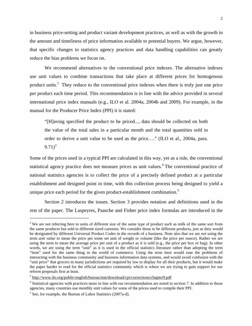
Substituting the period t unit value, ,tnp , for the price variable t
np in the basic
specifications for the Laspeyres and Paasche indexes given in (2) and (3), and redefining the
quantity variable as the summation over all transactions in the given period, we obtain,
respectively, the following expressions for what we call the hybrid Laspeyres index (the
HLaspeyres index for short)16
(12)
,0
n
,1nN
1n0n
N1n
0n
,0n
N1n
0n
,0n
,0n
,1n
N1n
0n
,0n
N1n
0n
,1n1,0
HLp
pS
qp
qp
p
p
qp
qpP
and for the hybrid Paasche index (the HPaasche index)
(13)
11
,0n
,1nN
1n1n
N1n
1n
,0n
N1n
1n
,1n1,0
HPp
pS
qp
qpP
.
Thus the hybrid Fisher index (the HFisher) is given by
(14) 2/11,0AP
1,0AL
1,0HF )PP(P .
The value share weights in (12) and (13), 0nS and 1
nS , are given for all n by
(15) ttn
tn R/RS ,
with tnR now given by (7) and where N
1ntn
t RR .
The HLaspeyres, HPaasche and HFisher indexes use unit values for the first stage of
aggregation, so they can explicitly accommodate a product being transacted at multiple prices
within a unit time period. They reduce to the basic formulas in situations in which there truly is
just one price per period for each product. From (12)-(14), we see too that the HLaspeyres,
HPaasche and HFisher indexes are summary metrics for relatives of average prices (i.e., what we
will refer to as unit value price relatives) defined as:
(16) )p/p( ,0n
,1n
.
16 The term “hybrid” was suggested to Marshall Reinsdorf by Harlan Lopez of the Central Bank of Nicaragua.

13
These unit value price relatives reduce to the usual price relatives given in (6) when there is just
one price per period for each product. Thus the HLaspeyres, HPaasche and HFisher formulas are
generalizations of the basic formulas.
Analysts who have estimated price indexes using raw scanner or other transactions level
data17 from merchants or from financial markets are, in fact, already accustomed to evaluating
price indexes based on unit value price relatives,18 but they have not always made this practice
explicit by spelling out the data processing specifics. By calling attention to how formulas (12)-
(16) depart from the corresponding basic formulas, and by providing terminology for these
practices, we hope to facilitate efforts aimed at finding practical solutions to the problems
statistical agencies face in dealing with the reality of multiple prices per product per period.
3.3 An Important Historical Clarification
We chose to label as “Hybrid” indexes the Laspeyres, Paasche and Fisher formulas given
in (12)-(14) above. But, in fact, these are the “true” Laspeyres, Paasche and Fisher indexes as
introduced by the original authors. Only one of the multiple authors of this paper (namely, Erwin
Diewert) had the language skills need to go back to the original German articles by Laspeyres
(1871) and Paasche (1874). However, Walsh (1901, 1921) and Fisher (1922) wrote in English
and are quite explicit that unit value prices and total quantities transacted in the given time period
and market place are the “right” p’s and q’s that should be used in a bilateral index number
formula at the first stage of aggregation over transactions that take place at different prices
within the period.
Of course, when authors put their creations into the public domain, they cannot control
how others alter what they originally proposed. It is clear that large numbers of authors have
defined and used the indexes as in (2)-(4) above, which are what we have labelled as the “Basic”
indexes. And official statistics agencies have typically defined and used the indexes in the form
we give subsequently (in (31)-(33)), and which we have labelled the “Conventional” indexes. It
17 By “raw” we mean transactions data not already aggregated over time. Providers of what is labelled as “transactions data” often, in fact, deliver data sets consisting of the total quantities transacted and the unit values for some unit time period such as a week. See, for instance, Nakamura, Nakamura and Nakamura (2011) for a study done using transactions data of this sort. 18 See, for example, Ivancic, Diewert and Fox (2011) and Nakamura, Nakamura and Nakamura (2011).

14
is in this context, and in the context of uses we make of the indexes subsequently in this paper,
that we refer to formulas (12)-(14) as “Hybrid” indexes.
3.4 Working with Grouped Transactions Data
Suppose we want to divide up the transactions for the N products covered by a price
index according to one or more auxiliary attributes. For transaction j for product n in period t, the
price and quantity are denoted here by j,tnp and j,t
nq . We can designate a total of C exhaustive
and mutually exclusive groups for the transactions: GC,,1G . For each group of transactions,
the total quantity and the average price (i.e., the group quantity and the group unit value) are
given, respectively, by
(17)
Gcj
j,tn
Gc,tn qq and Gc,t
nGcj
j,tn
j,tn
Gc,tn q/)qp(p
.
Hence for each product n, the overall quantity transacted in period t can be represented as:
(18)
GC
1GGcGcj
j,tn
GC,tn
1G,tn
tn qqqq .
The overall unit price for product n in period t can now be given as
(19) ,tnp
GC1GGc
Gc,tn
Gc,tn
tn
GC1GGc
Gc,tn
Gc,tn
tn
GC1GGc
GCj
j,tn
j,tn spq/)qp(q/)qp( ,
where for group GC,,1GGc , we have the following for the quantity shares, Gc,tns , for groups
GC,,1Gc we have
(20) tn
Gc,tn
Gc,tn q/qs with 1ss GC,t
n1G,t
n .
Note that the quantity shares defined in (20) can only be meaningfully computed when
the product units being added are homogeneous with respect to their primary attributes. With
this proviso, when the total quantity transacted in period t is computed as in (18) and the period t
unit value for each product n is computed as in (19), then the HLaspeyres, HPaasche and HFisher
formulas given in (12)-(14) can be evaluated. In other words, the only adjustment needed in this
grouped transactions case is to use (18) and (19), rather than (10) and (11), to compute the
quantity and price summary statistics.

15
3.5 A Formula for the Bias in Conventional Laspeyres, Paasche and Fisher Indexes
As noted, with some exceptions the conventional statistical agency practice is to collect
just one price to represent a product in an establishment in a time period. Without loss of
generality, we denote the one transaction used in the conventional index as transaction 1 (i.e., as
1j ). The full set of transactions in a given period t for each product n can then be divided into
two mutually exclusive and exhaustive groups, G1 and G2, with G1 containing the single
transaction used in compiling a conventional price index and G2 containing the rest of the
transactions, which are transactions ignored in the conventional way of compiling the index.
Hence for G1, the quantity and price summary statistics can be denoted, respectively, as
(21) 1,tn
1G,tn qq and 1,t
n1G,t
n pp ,
and, from (17), we see that for group G2 we have
(22)
2Gj
2G,tn
J2j
j,tn
2G,tn qqq
tn and 2G,t
nj,t
n2Gj
j,tn
2G,tn
j,tn
J2j
j,tn
2G,tn q/)qp(q/)qp(p
tn
,
where 2G,tnq is the quantity total and 2G,t
np is the unit value for the G2 transactions.
The total quantity transacted for each product n in period t is the sum of the transactions
quantities for the G1 and the G2 groups, so we have
(23) 2G,tn
1G,tn
2Gj
j,tn
1Gj
j,tn
J1j
j,tn
tn qqqqqq
tn
.
And, from the last expression in (19), the overall unit price for product n in period t is
(24) ,spspp G2t,n
G2t,n
G1t,n
G1t,n
,tn
where now for the quantity share statistics we have:
(25) tn
1G,tn
1G,tn q/qs and t
n2G,t
n2G,t
n q/qs with 1ss 2G,tn
1G,tn .
For our price index bias analyses in section 4, it will prove useful to define a factor
relating the average of the G2 transaction prices to the single G1 price. The product specific
discount factor, tnd , is defined such that one minus this discount factor is the factor of
proportionality relating the average for the ignored G2 prices to the G1 price:

16
(26) 1G,tn
tn
2G,tn p)d1(p .
When the average price for the G2 transactions for product n in period t is less than the
corresponding G1 price, then tnd will be strictly between 0 and 1. When the average for the G2
prices is greater than the G1 price, then tnd will be negative, making )d1( t
n greater than 1.
The overall average price can now be represented as follows for product n in period t:
(27)
.pout factoring after p)sd-(1
1ss here w spd-)ss(p
spd-spsp
(26)usingsp)d-1(sp
(24)using )spsp(p
1G,tn
1G,tn
G2t,n
tn
2G,tn
1G,tn
2G,tn
1G,tn
tn
2G,tn
1G,tn
1G,tn
2G,tn
1G,tn
tn
2G,tn
1G,tn
1G,tn
1G,tn
2G,tn
1G,tn
tn
1G,tn
1G,tn
2G,tn
2G,tn
1G,tn
1G,tn
,tn
We see from the last line of (27) that what we label as the price quote representativeness term,
given by )sd1( 2G,tn
tn , relates the unit value for all the period t transactions for product n to the
one price quote used when following conventional index making practice.
Now define a product specific price index representativeness factor 1,0n as the ratio of
the price quote representativeness terms for period 1 versus period 0:
(28) .sd1
sd12G,0
n0n
2G,1n
1n1,0
n
This price index representativeness factor equals 1 when the representativeness term has the
same value in both period 0 and period 1. So long as this factor is approximately equal to 1, then
the overall average price for product n is related in the same manner in both periods 0 and 1 to
the one price quote conventionally utilized each period. In contrast, values of 1,0n that are
appreciably different from 1 indicate that there is a difference between periods 0 and 1 in how
the overall average price relates to the price quote utilized. (Note that 1,0n exists and is positive
if there are at least two transactions per period; 2G,tns must be strictly less than 1 because G1 must
contain a transaction for some positive quantity in both time periods and tnd must be strictly less
than 1 since the average G2 price is positive in either time period.)

17
The last expression for the HLaspeyres price index given in (12) can now be restated to
incorporate the relative price index representativeness factor 1,0n :
(29)
.(28) using p
pS
p
psd1
sd1
S
(27) using p)sd1(
p)sd1(S
p
pSP
N1n 1G,0
n
1G,1n1,0
n0n
N1n 1G,0
n
1G,1n2G,0
n0n
2G,1n
1n
0n
N1n 1G,0
n2G,0
n0n
1G,1n
2G,1n
1n0
n,0
n
,1nN
1n0n
1,0HL
Similarly, the HPaasche price index given in (13) can be restated as
(30)
1
N1n
1
1G,0n
1G,1n1,0
n1n
1,0HP
p
pSP
.
The HFisher counterpart of (29) and (30) is still given by (14), but with the HLaspeyres and
HPaasche components now given by (29) and (30).
We are now ready to define the price index formulas we will refer to as conventional.19
To obtain the conventional Laspeyres price index ( 1,0CLP ), we substitute )p/p( 1G,0
n1G,1
n for
)p/p( ,0n
,1n
in the first expression for 1,0HLP given in (29), in accord with the conventional practice
of only using one price observation per product in each time period:
(31)
N
1n 1G,0n
1G,1n0
n1,0
CLp
pSP .
19 In defining these formulas, we ignore the important aspect of conventional practice that is the focus of the Lowe index literature: namely, that the data used in estimating the value shares is collected separately from the price information used in index making, and is not usually even for the same time periods. See Diewert (1993) and Balk (2008, chapter 1) for more on this issue.

18
Similarly, to obtain the conventional Paasche price index ( 1,0CPP ), we substitute )p/p( 1G,0
n1G,1
n for
)p/p( ,0n
,1n
in the first expression for 1,0HPP given in (30), again in accord with the conventional
practice of only using one price observation per product in each time period:
(32)
1
N1n
1
1G,0n
1G,1n1
n1,0
CPp
pSP
.
The conventional Fisher price index ( 1,0CFP ) is given by:
(33) 2/11,0CP
1,0CL
1,0CF )PP(P .
In the index number literature, the term “bias” refers to a systematic difference between
the result that would be obtained for some index in use or considered for use versus a specified
target index. To this point, we have only demonstrated the price index representativeness factor
as an outcome of sampling error: basing an index on one product item will yield a different
answer from using the entire population of product prices. In section 4 below, however, we
present reasons why the price of the selected item could have a systematically different
expectation from the population unit value. If we use ALP given in (29) as the target index, then
the bias of the conventional Laspeyres index given in (31) is:
(34)
1G,0n
1G,1n1,0
nN
1n0n1G,0
n
1G,1nN
1n0n
HLCL1,0
CL
p
pS
p
pS
PPB
1G,0
n
1G,1nN
1n0n
1,0n
p
pS)1(
1G,0
n
1G,1n0
nN
1n 2G,0n
0n
2G,0n
0n
2G,1n
1n
p
pS
sd1
sdsd using (28).
Similarly, using (32) and (30), for the conventional Paasche index, the bias is:

19
(35) 1
N1n
1
1G,0n
1G,1n1,0
n1n
1
N1n
1
1G,0n
1G,1n1
n
HPCP1,0
CP
p
pS
p
pS
PPB
It is cumbersome to develop a bias formula for the conventional Fisher index given in
(33). However, as Diewert and Nakamura (2010/2011, appendix) explain, it is straightforward to
develop formulas for the differences between the arithmetic averages of the Laspeyres and
Paasche components for the conventional and for the target Laspeyres and Paasche components,
respectively, of the conventional and the target Fisher indexes. 20 Thus the bias of the
conventional Fisher index can be approximated by
(36) ]2/)PP[(]2/)PP[(PPB 1,0HP
1,0HL
1,0CP
1,0CL
1,0HF
1,0CF
1,0CF .
4. Different Sorts of Price Index Selection Bias
In the following section, we show how expression (34) can be used to represent and
provide a framework of analysis for multiple sorts of price index bias. We focus here on the
Laspeyres bias formula because the BLS (and other statistical agencies) mostly use the
Laspeyres index in their inflation measurement programs. However, comparable results for the
Paasche and Fisher formulas can be derived starting instead from (35) or (36).
4.1 Outlet Substitution Bias in the CPI
For the CPI, the BLS collects prices from selected retail outlets. In an effort to control for
possible price determining factors that can differ even for the same commercial product (i.e., to
control for what we call auxiliary product unit attributes), the BLS only forms price relatives for
product units sold at the same retail outlet (see Greenlees and McClelland, 2011). Suppose,
however, that households mostly care about what they must pay for products characterized by
their primary attributes (including the brand and producer), and hence shift their expenditures
among retail outlets in response to advertising about pricing policies and temporary promotional
sales. The benefits of this sort of price-informed shopping in terms of the prices actually paid for
20 For more, see Diewert and Nakamura (2010/2011, appendix).

20
the products used by any one consumer will be missed by a practice of only pairing prices for the
same retail outlet in forming price relatives. If the ratio of the average price paid to the price
used in the index is falling because opportunities for paying discounted prices are increasing, the
conventional index will be upward biased.
The potential for outlet-specific price relative evaluation to cause CPI price index bias
was noted decades ago. In a 1962 report, Edward Denison raised the concern that, in his words,
“revolutionary changes in establishment type that have taken place in retail trade” may have
caused “a substantial upward bias” in the CPI (p. 162).21
Marshall Reinsdorf empirically investigated Denison’s CPI bias hypothesis. The BLS
produces average price (AP) series for selected food groups. These are unit value series for
certain food categories, though not for strictly homogenous products as we advocate. Reinsdorf
(1993) compared selected AP series for food and gasoline with the corresponding CPI
component series. He discovered that from 1980 to 1990, the CPI and AP series for comparable
products diverged by roughly 2 percentage points a year, with the CPI series rising faster than
the AP series, as would be expected if the CPI systematically fails to capture the benefits to
consumers of price-motivated retail outlet switching. These empirical results captured the
attention of Erwin Diewert, inspiring him to derive a formula for what he called the outlet
substitution bias problem (Diewert, 1998).
Reinsdorf (1999a) later found that formula bias in the CPI caused part of the divergences
between CPIs and corresponding AP series, so the outlet substitution effects turned out to be
0.25 percent per year for both food and gasoline. The combined efforts of Reinsdorf and Diewert
then galvanized other economists and price statisticians to take the outlet substitution bias
problem seriously.22
If a significant number of consumers regularly switch where they shop among multiple
retail outlets depending on the product prices each is currently offering, then we would expect
tnd defined in (26) to be strictly between 0 and 1 in value for both periods 0 and 1. This alone,
21 For more on the practical aspects of these “revolutionary changes” that Denison (1962) noted and foresaw, see Brown (1997), Garg et al. (1999), Freeman et al. (2011), Hausman and Leibtag (2007, 2010), and Senker (1990). 22 Important papers on this topic include Moulton (1993, 1996a, 1996b), Hausman (2003), Hausman and Leibtag (2007, 2010), and Greenlees and McClelland (2011). Also, White (2000) presents related evidence for Canada.

21
however, will not cause a bias problem. We see from (34) that the key question is whether the
term 2G,tn
tnsd has been changing in value over time. If the value of this term happened to
stabilize, there would be no outlet substitution bias then. We believe, however, that the G2
quantity share ( 2G,tns ) has been growing over time for two sorts of complimentary reasons. The
first is that modern information technologies have made it cheaper and easier for retailers to hold
temporary promotional sales, which tend to generate high demand. The second is that there have
been steady improvements in consumer access to current information about retail prices at
different outlets in their market area including now even smart phone geo-targeted advertising.
Hence we expect the Laspeyres index bias given by (34) to be positive.
4.2 CPI Promotional Sale Bias
Outlet substitution bias discussed above can result from a failure to capture a growing
trend for consumers to take advantage of temporary sale and other price differences among retail
outlets. However, even at for the same retail outlet, units of a product are often sold at both
regular and promotional sale prices within a month, which is the unit time period for the CPI.
The frequency of temporary sales is believed to have been increasing in the US. The information
available to consumers about sale pricing has been steadily expanding too, presumably allowing
consumers to take progressively greater advantage of temporary promotional sale prices.23
The BLS collects and uses for the CPI whatever prices are in effect at the time the price
quotes are collected from each selected retail outlet, regardless of whether the prices are
identified as “sale” or “regular” prices.24 Temporary sales are believed to be in effect for any one
product at any one outlet for less than half of the days or hours of business. Hence the value of
tnd is expected to be predominantly between 0 and 1. Nevertheless, because the capture of
regular or sale prices is random, the value of can be either positive or negative.
23 For more on the importance of temporary sales for explaining retail price dynamics, see Pashigian (1988), Pesendorfer (2002), and Nakamura and Steinsson (2008, 2012). 24 The same is true for Statistics Canada (1996, p. 5): “Since the Consumer Price Index is designed to measure price changes experienced by Canadian consumers, the prices used in the CPI are those that any consumer would have to pay on the day of the survey. This means that if an item is on sale, the sale price is collected.” The BLS does, however, have other special procedures for handling sale prices of apparel at the end of the selling season.

22
The volumes sold at promotional sale prices tend to be large and, as already stated, the
frequency of temporary sales is believed to have been rising in the US at least. As is evident
from equation (28), the sign of the change in the term 2G,tn
tnsd determines the sign of promotions
bias.25 Because the US CPI includes sales prices in proportion to the percent of time in which
they are offered, increased frequency of sales could result in either a rise or a fall in this term. A
fall would occur if the increased frequency of sale price offerings increased the relative
frequency of sale prices being selected for the CPI by more than it increased the relative
frequency of sale prices being paid by consumers. On the other hand, if consumers’ costs of
acquiring information fall, the term would likely rise, implying positive promotions bias.
Information costs have, indeed, fallen, so promotions bias may be positive on average.26
4.3 Sourcing Substitution Biases in the PPI and MPI
Finding cheaper input sources and then making sourcing substitutions is a prevalent
strategy for lowering business costs. Empirical evidence suggests that this sort of supplier
switching behavior plays an economically important role in the survival and growth of new firms
(e.g., Foster, Haltiwanger, and Syverson, 2008; Bergin, Feenstra and Hanson, 2009).27 If both the
old and the new suppliers are domestic, it is the uses of the Producer Price Index (PPI) as a
deflator for inputs that can be affected. If both the old and the new suppliers are foreign, it is the
Import Price Index (MPI) that can be affected.
For both the PPI and MPI cases, we would expect the values of tnd in (26) to be strictly
between 0 and 1. Moreover, we would expect the G2 quantity share ( 2G,tns ) to have been
growing over time due to expanding information availability about suppliers and their prices,
25 The statistical agencies for some US trading partners such as Japan exclude temporary sale prices in compiling their Consumer Price Index (CPI). For example, price collectors are instructed by the Statistics Bureau of Japan not to collect sale prices. More specifically, price collectors are instructed that “the following prices are excluded: Extra-low prices due to the bargain sales, clearance sales, discount sales, etc., which are held for less than seven days,” Statistics Bureau of Japan (2012, p. 3, item 10). See also Imai, Shimizu and Watanabe (2012). This methodology difference could definitely affect inter-nation comparisons of inflation, economic growth and well being, and formula (34) can be useful for understanding these effects. 26 We thank Brent Moulton for comments that greatly improved this section of the paper. 27 Supply chain models like what Oberfield (2013) specifies assume that much of what typically is measured as technical progress in fact reflects the cost savings from supplier switches.

23
enabling purchasers to take greater advantage of lower price offers. Hence we would expect
positive biases in the relevant price indexes from sourcing substitutions. Houseman et al. (2011)
provide relevant empirical evidence for the MPI case.
We next provide a simple example illustrating this bias problem for the MPI. Then we go
on to take up two other possible sorts of producer sourcing changes that may cause bias problems.
4.4 An Example of MPI Sourcing Substitution Bias Due to Import Sourcing Switches
Here we distinguish a supplier (k) from a buyer ( k ). For our example, businesses 1 and
2 are foreign suppliers (hence 2,1k ) and businesses 3 and 4 are domestic buyers (hence
4,3k ) for a single product. The quantities and prices are denoted by tk,kq and t
k,kp . With
only one product, a Laspeyres (or Paasche or Fisher) price index reduces simply to a ratio of a
single price or average price for the one product in each of the two time periods for the price
index.
Table 1. Value Flows for the Four Businesses
Output flows Input flows
Business 1 Business 2 Business 3 Business 4
Period 0 value flows
03,1
03,1 qp 0
4,20
4,2 qp 03,1
03,1 qp 0
4,20
4,2 qp
Period 1 value flows
13,1
13,1 qp 1
4,21
4,21
3,21
3,2 qpqp 13,2
13,2
13,1
13,1 qpqp 1
4,21
4,2 qp
The value flows summarized in table 1 reflect the following specifics:
Business 1 is a developed country supplier to business 3, with this supply arrangement
having been in place already for more than two periods as of the start of period 0 for this
example.
Business 2 is a cheaper, developing country supplier that has a supply arrangement with
business 4 that was in place already for more than two periods as of the start of period 0.

24
Business 3 purchases from business 1 in both periods 0 and 1. In period 1, business 3 also
enters into a new purchasing relationship with the low cost supplier 2. This is a simplified
situation of the sort explored empirically by Houseman et al. (2011). What a new supplier
charges has no effect on the “conventional” price index.
Business 4 has had an ongoing purchasing relationship with business 2, and continues to
buy exclusively from business 2 in periods 0 and 1.
The following inequalities hold: 0pp 04,2
03,1 , 0pp 1
4,21
3,1 , 0pp 13,2
13,1 .
The price indexes for domestic businesses 3 and 4 can be regarded as MPI index series.
The conventional price index for business 4, )4(CLP , is the same as our hybrid Laspeyres
target price index for that business, )4(HLP , because business 4 uses just one supplier each period.
There is no bias problem for )4(CLP . For this case, the conventional price index equals the target
price index:
(37) )4(HL
04,2
14,2
)4(CL Pp/pP .
In contrast, we can show that the conventional price index for business 3 is biased, and
we can show what the bias depends on. For business 3, the conventional price index is:
(38) i1p/pP 03,1
13,1
)3(CL ,
where )i1( is the measured inflation rate using this conventional price index. This conventional
price index takes no account of the fact that in period 1, business 3 not only bought from
business 1 but also used a new supplier, business 2. In contrast, and under our assumption that
business 3 views the products from the two suppliers as equivalent, the specified target index for
business 3 uses the information for all the transactions in period 1. This price information is
summarized in period 1 by the unit value, 13,p ; i.e., we have
(39) 13,2
13,2
13,1
13,11
3,21
3,1
13,2
13,2
13,1
13,11
3, spspqq
qpqpp
,
where

25
(40) )qq(
qs
13,2
13,1
13,11
3,1
, )qq(
qs
13,2
13,1
13,21
3,2
, and 1ss 13,2
13,1 .
Hence the target output price index for business 3 is given by
(41) 13,2
03,1
13,2
13,1
03,1
13,1
03,1
13
)3(HL s)p/p(s)p/p(p/uP .
It is the price charged by the lower priced supplier, business 2, that is ignored by the
conventional price index for business 3. The price charged by business 2 is what constitutes the
G2 group price for this example, whereas 13,1p is the G1 price. Using (26), we have
(42) 13,2
113,1 p)d1(p using (38) and (42),
where 1d0 1 . In period 0, there is only the one supplier for business 3. Hence applying (34)
yields:28
(43)
(38). using 0)i1(sd
p
psd
PPB
13,2
1
03,1
13,11
3,21
)3(HL
)3(CL
1,0CL
The last two lines of (43) are convenient alternative expressions for the sourcing substitution bias
of )3(CLP .
We note that the last expression in (43) is the same as equation (12) in Diewert and
Nakamura (2010/2011).29 This bias is seen to depend on:
The rate of price inflation as measured by the conventional index;
The proportional cost advantage of any ignored supply source(s); and,
The quantity share for any ignored supply source(s).
28 Note that the terms in (34) involving 0nd drop out of the final expression in this case, and also here we have
1S0 because, in period 0, there is only the one supplier for business 3 charging a single price. 29 Equation (2) in Reinsdorf and Yuskavage (2014) modifies this formula to use a value share weight instead of a quantity share by multiplying by a factor that is between 1 and 1/d1. Also, Houseman et al. (2010, p. 70) derive a formula for calculating quantity shares from value shares and the discount d1. A related formula for outlet substitution bias is found in Diewert (1998, p. 51).

26
If estimates can be made for the above factors, then a rough approximation to the bias given in
(43) can be made using this formula, which is a special case of our general bias formula (34).
4.5 Domestic to Foreign Supplier Switches and a Proposed True Input Price Index (IPI)
We next consider the case of a business that switches from using a domestic supplier to a
foreign one, thereby benefitting from an input cost decrease. Neither the PPI nor the MPI can
capture the cost savings from this sort of a sourcing substitution. The PPI’s domain of definition
does not include imports, and the MPI measures price changes beginning in the second month in
which a newly selected imported product is observed. The resulting price index coverage gap is
worrisome since most of the increase in the relative importance of trade in the US economy is
accounted for by the expansion of imports of intermediate products.30
The pricing gap between the PPI and the MPI programs could be closed by creating a true
Input Price Index (IPI) program that is defined to measure the inflation experience of producers
in buying their inputs from all sources: foreign as well as domestic. In this case, the price
evolutions measured should include those associated with shifts in purchase shares from more to
less expensive domestic producers, and from more to less expensive foreign producers, as well as
from domestic to cheaper foreign producers.
The BLS has put forward a plan for a true IPI (Alterman 2008, 2009, 2013). With an IPI,
a newly imported product that matches the primary attributes of a domestically supplied product
could be brought into the IPI as a directly comparable substitute. Also, in principle, the purchaser
of the inputs would be able to report the price per unit irrespective of the sources for inputs they
treat as homogeneous in terms of what is done with the product purchases.
However, if the current BLS practice of not averaging prices over units of a product with
different prices and from different suppliers is adopted for the IPI program too, then the new IPI
could also be subject to sourcing substitution bias.31 This IPI bias could be represented using (34)
in the same manner as for the PPI and MPI cases except that purchases for domestic as well as
30 See Yuskavage, Strassner, and Mediros (2008), Kurz and Lengermann (2008), and Eldridge and Harper (2010). 31 This point was independently noted by both Diewert and Nakamura (2010/2011) and by Reinsdorf and Yuskavage (2014).

27
imported inputs would now be covered. For the same sorts of reasons discussed above for the
PPI and MPI, we would expect this bias problem to be positive and growing.32
4.6 Inflation Measurement Problems Due to the Initial Switch to Outsourcing
When a business switches from in-house production to procurement of an intermediate
input, this is usually done in hopes of realizing cost savings. The fact that this sort of cost savings
will not be picked up by the PPI or MPI programs is sometimes treated as an aspect of the new
goods price index bias problem even if there is nothing new in terms of the input in question. We
note, however, that there will usually be no way for a business to make this sort of a change
without alterations to the operating processes of the business. Alternatively, therefore, this sort of
sourcing change might be viewed as a business technology change that should be counted as a
contribution to productivity growth. Nevertheless, regardless of which of these perspectives is
adopted, this sort of change is outside the scope of this paper.
5. Five Sorts of Barriers to Adoption of Unit Values for Official Statistics Purposes
The target indexes we recommend incorporate unit values. As we have noted, there are
impediments to the adoption of indexes like this by statistics agencies in their official published
series. Here we deal with what we see as the main impediments grouped under five subheadings.
5.1 Impediment 1: Bad Reputation Due to Historical Misuse of Unit Value Indexes
The Price Statistics Review Committee chaired by George Stigler, also known as the
Stigler Committee, considered the relative merits of unit value versus what is referred to as
specification pricing and recommended the latter. Under the heading of “Specification vs. Unit
Pricing,” the Stigler Committee report33 states that:
“In 1934, the Bureau of Labor Statistics adopted ‘specification’ pricing, and since
then has sought to price narrowly defined commodities and services to obtain
32 An additional conceptual test is international aggregation as in Maddison (2001). The sum of world GDP should be a consistent measure of world investment and consumption; this implies that exports and imports (with shipping costs) equate across nations in real terms. Eliminating sourcing biases moves us toward an ability to meet this test. 33 See the Price Statistics Review Committee of the National Bureau of Economic Research (1961).

28
price relatives for price indexes…. The Committee believes that in principle the
specification method of pricing is the appropriate method for price indexes. The
changing unit values of a broad class of goods (say shirts or automobiles) reflect
both the changes in prices of comparable items and the shifting composition of
lower and higher quality items.” [italics added]
Note, however, that the Stigler Committee’s opposition to unit values did not arise in the context
of price collection for carefully and very narrowly specified products as we are recommending;
rather it arose in the context of prices collected for what nowadays would be viewed as very
broadly specified products.
The Stigler Committee report recommended the use of probability sampling methods by
the BLS, and these methods led to heterogeneous samples of items being selected. In addition,
back then, the price of new cars was based on the average of what were referred to as the “low
priced three” makes of automobile (Chevrolet, Ford, and Plymouth), with no adjustment for
quality as the models evolved over time. The Committee report particularly was concerned that,
“In the case of the Farm Indexes the classes over which unit values are computed are still often
too wide (p. 33).” An accompanying study by Rees (1961) argued that the Farm Index measure
of rugs, which did not specify the fiber content, failed to capture a substantial rise in the price of
wool rugs reflected in the BLS data (and in Sears and Ward catalogs) because it increasingly
captured the pricing of wool-rayon blend rugs (pp.150-153).34 Similarly, the old US Census
Bureau unit value indexes for imports and exports were based on customs administrative data for
very broad product categories. As a result, the Census Bureau unit value average prices were
clearly subject to mix shifts.
As part of its response to the Stigler Report, in 1973 the BLS began producing
rudimentary versions of an Import Price Index (MPI) and an Export Price Index (XPI) using
price quotes and value share weights produced by methods similar to those used for the PPI
program. Full coverage of import and export goods categories was achieved by 1982 for the MPI
and XPI.35 Nevertheless, the Census Bureau unit value indexes were not discontinued until July
1989. Alterman (1991) takes advantage of data from the overlap years to conduct a comparative
34 From 1948 to 1959, the relevant BLS price index services and Sears and Ward prices grew 50 percent, whereas the Farm Index series grew less than 10 percent. 35 See also Silver (2010).

29
empirical study of the Census unit value indexes versus the MPI and XPI produced by BLS. That
study notes that if unit values are computed for what, in fact, are different products, then those
price indexes will reflect not only the underlying price changes, but also any changes in product
mix as well. By way of example, he goes on to state that if there were a market shift, say, “from
cheap economy cars to expensive luxury cars, the unit value of the commodity (autos) will
increase, even if all prices for individual products remain constant.” This clarifying remark
makes it clear that Alterman, in his 1991 paper, is referring to the commodity categories the
Bureau of Census used in constructing their unit value indexes rather than to precisely and very
narrowly defined products. Alterman’s remark was true for the customs data that the Bureau of
Census used in constructing their unit value indexes but does not pertain to our proposals.
Alterman (1991) also reports an interesting anomaly along with his other findings:
“In comparing price trends of imported products, the BLS series, surprisingly,
registered a consistently higher rate of increase between 1985 and 1989. Between
March 1985 and June 1989 the BLS index rose 20.8 percent, while the equivalent
unit-value index increased just 13.7 percent…. With the exception of motor
vehicles, the major import components -- foods, feeds, and beverages, industrial
supplies and materials, capital goods, and consumer goods -- all show larger
increases in the BLS series than in the unit value series. The most dramatic
difference between the two series is found in the comparison for imported
consumer goods. Between March 1985 and June 1989 the BLS series recorded a
30.7 percent increase, while the comparable unit-value series rose just 10.3
percent.” [italics added]
As Alterman explains, his discovery that the Census Bureau unit value series show smaller price
increases for imports than the MPI contradicts a common presumption about the nature of unit
value indexes. This is the presumption that quality levels tend to rise over time, so that the failure
to adjust for product mix changes within the product categories for which prices are being
averaged will typically cause unit value indexes based on broad product categories to overstate
the true price increases.36
36 Alterman (1991) proposes and checks out other possible explanations as well for the results he observed, but reports that those other hypotheses were rejected by the data.

30
We, however, now suspect that what Alterman identified as an “anomalous” result is
likely a manifestation of sourcing substitution bias in the MPI: a problem that would not have
affected the Census unit value series in the same way. In particular, the MPI produced by the
BLS could not capture direct cost savings that buyers achieved by switching to lower cost
suppliers. In contrast, the old Census unit value series probably did capture at least some of those
price motivated buying switches among products sharing the same, or almost the same, primary
attributes.37
5.2 Impediment 2: Questions Regarding the Proper Treatment of Auxiliary Attributes
Producers of mass marketed products try to ensure the consistency of the units of what
they label as being the same commercial product. Producers usually want it to be the case that
units of what they label as “a product” can be advertised and sold interchangeably. For example,
a 10.75-ounce can of Campbell’s tomato soup, as this is defined by the company that owns the
brand, is intended by Campbell’s to be the same product no matter when, where or how a can of
the soup is purchased. As noted, however, units of a homogeneous product that all have the same
primary attributes can acquire different auxiliary attributes such as having been sold at regular
price or during a temporary promotional sale, or at a neighborhood convenience store versus a
superstore.
And yet, when it comes to using units of a product (e.g., cans of soup or tins of tuna)
purchased, say, from different outlets to take advantage of price promotions, typically no account
is taken of the foregone effort or time of the family member who did the shopping in terms of
how the product units are utilized. This is in line with current practices for compiling the Gross
Domestic Product (GDP). That aggregate is compiled for the US by the Bureau of Economic
Analysis (BEA) following the guidelines of the System of National Accounts (SNA). It is
explicit in the SNA that no account is taken of unpaid time expenditures of household members,
whether for picking up groceries at a superstore, rather than, say, a nearby convenience store, or
37 Written comments by Pinelopi Koujianou Goldberg on Nakamura and Steinsson (2012), shared with us by those authors, led us to see this point, and made us aware that similar issues may affect a variety of other studies and views on changes over time in price flexibility and related issues for the US economy and for international comparisons.

31
for any other activity.38 Moreover, the nominal value of the consumption aggregate includes all
sales of consumer products at the prices for which they were, in fact, purchased. One main
purpose of the CPI program is to provide components to be used for constructing deflators for
the consumption aggregate of the GDP.
We can, nevertheless, see reasons for wanting to hold a variety of auxiliary attributes
constant in estimating the price relatives that are used in compiling a price index. After all,
customers are willing to pay more per unit for the soup cans sold in a convenience store, and, in
that sense, those cans of soup are definitely of “higher quality” than lower priced units of the
product sold at a discount super store. If that product differentiation is adopted for price quote
collection purposes, however, then it is important for the auxiliary product attributes to be taken
into account as well in collecting the data for and in producing the product-specific value-share
weights for the price index. The question of how auxiliary product unit attributes should be
treated is deep, and largely beyond the scope of this paper.
5.3 Impediment 3: Producer Goods with Different UPCs but the Same Primary
Attributes
The mechanics of price measurement for producer goods are greatly simplified when the
products can be specified as individual product UPCs or pre-defined groups of these. It is the
primary product characteristics that usually matter for how product units are utilized in a
production process, and differences in primary attributes are always reflected in different UPCs.
Nevertheless, UPCs for product units sometimes differ even though the product units are
identical for practical purposes. For example, many large manufacturers issue precise
specifications for needed intermediate products, and then purposely select multiple suppliers
from among the businesses that bid on the supply contract opportunity. If intermediate product
units are produced according to identically the same specifications, but by different producers,
the product units from each producer will have producer-specific UPCs regardless of whether
there is any difference in any product attribute other than the identity of the producer. For price
index compilation purposes, units of products that are not treated differently by the final user
should usually be treated as the same product even when their UPCs may differ.
38 http://unstats.un.org/unsd/nationalaccount/

32
When the same product can have more than one UPC, those UPCs should be grouped
together and a single unit value price should be computed for the group each period. Defining
classification systems of UPCs can be a laborious process, however. In addition, if a producer
indicates that the product units from different suppliers are used or sold in the same way except
for some allowance for a quality difference (e.g., purchase order adjustments to allow for
supplier specific defect rates), then the producer could also be asked to report and evaluate the
quality difference, and that information could be used in implementing quality adjustments so
that the product units from the different suppliers can all be treated as units of the same constant
quality product.
5.4 Impediment 4: Consumer Products Sharing Primary Attributes but Not UPCs
Concerns have also been raised regarding the inflation measurement implications of a
growing proliferation of retail products with different UPCs even when the producer is the same
and the primary product attribute differences are trivial. One reason for this proliferation may be
that producers supplying retail products fear that their customers may switch to buying the
products of competitors if they raise their prices in an obvious way. Hence they instead bring out
new versions of the product that are minor variants on existing ones: variants advertised as being
new and improved and that are offered at increased prices that yield higher profit margins. The
corresponding old versions may then be discontinued.39
Another reason for the introduction by a producer of a new product that intentionally has
primary attributes that are highly similar to the attributes of an existing product may be a desire
to take market share from competitors with successful products. In these cases, the producer
wants the new product to differ enough from the old one to avoid successful trademark or patent
infringement lawsuits, but hopes that potential users will judge the new product to be the same
(or better) than the old one they were purchasing. For example, large grocery store chains often
introduce their own “private label” variants of popular established brand name products.
Similarly, clothing makers often try to bring out styles like those of popular designers. And
pharmaceutical companies often try to find ways of producing drugs with the same or better
effectiveness as the successful drugs produced by competitors. Foreign producers seeking to
39 See Nakamura and Steinsson (2008, 2012).
33
break into or expand in the US domestic market are another source of products with different
UPCs but that are deliberately similar to existing products in terms of the primary attributes.
Conversely, but equivalently for measurement purposes, a producer may have the goal of
maintaining a constant price by replacing a product with another that is less costly to produce.
Examples of the type often cited in the media would be the substitution of a slightly smaller
chocolate bar or package of coffee, with a new UPC, in lieu of raising the product price. Again,
such a strategy can make it difficult for the statistical agency to identify and measure the quality-
adjusted price increase.
Although statistical agencies like BLS do not average over changing sets of multiple
price quotes for individual products, for price change to be measured correctly, unit values are
sometimes defined in BLS price index programs to encompass multiple UPCs that represent the
same product. The task of determining when consumer products with different UPCs are, in fact,
sufficiently similar that they should be treated as the same for inflation measurement purposes
may be harder than the corresponding problem discussed above for producer products. There are
three reasons for this:
Consumers are far more numerous than producers, and they generally each buy much
smaller amounts than producers purchasing intermediate products. Hence the product use
views and experiences of much larger user groups would need to be considered to follow
an approach for consumers like what we suggest above for producers.
Producers inevitably keep and analyze data about the performance of units of an
intermediate product that are obtained from different suppliers. Consumers, on the other
hand, are not usually in a position to systematically note primary attribute quality
differences for similar product units from different producers.
Producer products that are similar enough that it might make sense to consider them as
being the same product were often requested by the purchaser. Thus the attempted
sameness is an openly declared objective to satisfy specifications issued by the purchaser.
In contrast, sameness in the consumer case that results from an effort to expand or enter
into a market by competing with the product of a competitor is usually illegal if the
duplication is exact. Hence, for consumer products, design work is needed to produce a
similar product that is nonetheless sufficiently different so that allegations of patent

34
infringement can be defended against. Foreign suppliers trying to gain market share from
domestic producers of consumer products often invest heavily in that sort of product
design work. A great deal of effort can go into legally producing an almost identical
product to one that already is being sold by some other producer.
Even when a very similar new product is developed by a producer as an alternative for
one of their own established products, perhaps in the hopes of being able to use the new product
as a means of making a de facto price adjustment, design work is usually required. This is so no
matter how small the differences may seem in terms of the primary product attributes. From
some perspectives, product development should be treated as part of productivity growth rather
than as a price change mechanism. Hence maybe these products truly should be treated as new
products rather than as quality adjusted old products. Kaplan and Menzio (2014) offer data on
the distribution of prices across similar products as well as within UPCs; their analysis sheds
some light on the relative importance of alternative product specification methods. However, we
do not attempt to provide answers here to these difficult questions.
Nevertheless, the issue of when and how to average prices over units of consumer
products with very similar primary attributes, as is now sometimes done on the consumer side
using hedonic and other quality adjustment methods, must be faced whether or not our
recommendation to use unit value price indexes is adopted. BLS is already engaged on an
ongoing basis in deciding when different product versions are similar enough to be treated as the
same thing, and those important efforts are outside of the scope of this paper and are not covered
here.
5.5 Impediment 5: A Need to Change Current Data Collection Arrangements
The most straightforward impediment to conquer might be the most serious. The
information requirements for a unit value price approach based on narrowly defined products are
much larger than for the approaches used for conventional price indexes. Nevertheless, private
businesses have paved the way. Businesses formerly carried out their decision making and
forecasting using sample and other sorts of incomplete information for their own transactions. In
contrast, modern big businesses strive to operate with full, real time transactional visibility.
35
Thus the nature of the needed changes at the BLS and other national statistics agencies
can be seen from the way in which large private sector businesses have remade their data
systems over the recent decades and have then also remade their business processes to utilize
their improved information capabilities. The needed hardware and software have been developed.
Nevertheless, moving a national statistics agency into a position of roughly equivalent data
storage and handling capabilities with what big companies now have will require large budget
allocations and substantial investments in training and hiring people with the needed capabilities.
Private sector data system experts do not have official statistics expertise, and those already with
the statistical agencies have had no opportunity to master data capture, warehousing and
utilization methods of the sort that have become common for big businesses, or the intricacies of
Universal Product Codes (the UPCs).40
It is instructive to briefly examine the steps that the private sector had to take to attain
their modern data handling capabilities. The 1961 Stigler Report was written before the business
world had UPCs. Indeed, for most of this century, as stores got bigger and varieties multiplied,
the only way for a grocer or other retailer to find out what was in stock was by physically
counting all the cans, boxes, and bags. The achievement of widespread use of UPCs was the
result of sustained business world efforts of many sorts. A machine readable product code design
had to be devised and agreed on. Equipment for cost effectively reading the product codes and
for storing and processing the product code data had to be invented, produced, purchased and put
to use by businesses. A product code numbering system had to be invented and agreed on. And
an organization had to be developed to oversee the assignment and use of product codes. Also,
business processes had to be redesigned to make use of the product code data.
More than a decade before the Stigler Report was written, Bernard Silver and Norman
Joseph Woodland developed and in 1952 were granted a patent for a barcode design consisting
of concentric circles that could be scanned from any direction. However, without a cheap, fast
and convenient way to read and record barcode data, their invention could not be put to applied
use. The development of cheap lasers and integrated circuits in the 1960s made barcode scanners
and barcode data handling potentially affordable for retailers. However, the original Silver-
40 There is an even larger knowledge gap opening up between the business world and the official statistics agencies as the business world now begins to move from UPCs and bar code scanners to Electronic Product Code (EPC) and Radio Frequency Identification (RFID) usage. See Roberti (2005) for more on the nature and reasons for this continuing evolution.

36
Woodland “bulls eye” barcode design performed poorly in an important field test. Also, there
was the challenge still to be met of getting all needed participants to more forward together.
In the early 1970s, IBM researcher George J. Laurer devised a new barcode design for
which the field test results were acceptable. He then succeeded as well in getting the US
Supermarket Ad Hoc Committee interested in what was named the IBM Uniform Product Code
(UPC) system.41 On April 3, 1973, the Ad Hoc Committee voted to accept the symbol proposed
by IBM.
Standardization made it worth the expense for manufacturers to put bar codes on their
packages and for printers to develop the needed new ink types, plates, and other necessities for
reproducing the code with the accuracy required for the UPC scanners, and the Ad Hoc
Committee succeeded in bringing the grocery industry and other needed participants together to
implement UPC scanning at the point of sale (POS). This included agreement on a standardized
system for assigning and retiring barcode product numbers. The nonprofit Uniform Code
Council (UCC) was established. Businesses applied for registration with the UCC, which
eventually changed its name to Global Standards One (GS1).42 Each business that was accepted
as a registered member began paying an annual fee and was then issued a manufacturer
identification number and given training on how to register their products and to assign and retire
UPCs as needed.
Use of scanners grew slowly at first. In 1978 less than one percent of grocery stores
nationwide had scanners. By mid-1981 the figure was 10 percent. Three years later it was 33
percent. And by 1999, it was already over 60 percent.43
GS1 today manages what is collectively referred to as the Global Trade Item Number
(GTIN) System which includes the UPCs.44 The official GS1 member organization for the US is
now called GS1 US. The modern logistics, inventory management, and pricing and advertising
operations of businesses of many sorts, especially including grocers and general merchandise
41 The Ad Hoc Committee consisted primarily of Presidents, Vice-Presidents, and CEOs who were selected from manufacturers, distributors, and retailers so as to insure that the interests of all parts of the grocery supply chain were represented. In addition to being corporate executives, the individuals selected for the Committee had significant knowledge, respect, and influence within the entire industry. 42 http://www.upccode.net/upc-guide/uniform-code-council.html 43 For more on this history, see Kennedy (2013). 44 http://www.gs1.org/epcglobal/about
37
retailers, would be inconceivable without the information derived from tracking product units
identified by UPCs.
In 1999, the Supermarket Ad Hoc Committee commissioned PriceWaterhouseCoopers to
make a report examining the extent to which the claims of the original Ad Hoc Committee
business plan had materialized (Garg, Jones and Sheedy, 1999). The resulting report finds that
the direct savings from barcode adoption proved greater than originally projected (i.e., savings at
the checkout counter). The report also finds, however, that it was the general merchandise
companies that managed to most fully realize the projected indirect savings from barcode
scanning rather than the supermarkets, and argues that the supermarkets have been losing market
share to super stores because of this reality. The indirect savings, which had been envisioned by
the original Ad Hoc Committee, pertain to business functions such as inventory management.
We see Walmart as the most notable example of this last point.
From 1973 on, as grocery and other retail chain stores grew, the chains almost all
established semi-autonomous regional data centers that collected and processed barcode scanner
data. The reason for the regional data centers that most chains created and many still have is that
the volume of the barcode data seemed too large for processing in a single data warehouse for
even a mid-sized chain store. Nevertheless, in 1979 Walmart built an initial company-wide data
warehouse (Metters and Walton, 2007). Walmart was also the first large retailer to give its
suppliers point-of-sale (POS) and inventory data for their products, thereby helping them reduce
costs due to under or over producing. Walmart recognized that by sharing this information with
its supply chain partners, they could all gain from improved coordination.
To improve the reliability of access to its data warehouse, in 1987, Walmart also built the
world’s largest private sector satellite communications system. Then in 1991, the company
reportedly spent $4 billion more to create their new Retail Link company-wide data warehouse.
Nowadays, Walmart suppliers are able to monitor in almost real time how their products are
selling on Walmart store shelves everywhere that Walmart carries their products. The POS data
is credited with enabling Walmart suppliers to reduce their inventories, shorten their lead times,
and increase their profitability. Also, with product items being electronically identified at the
checkout counters and with financial as well as physical inventory records being updated on an
on-going almost real-time basis, store managers in Walmart outlets everywhere as well as those
in the company headquarters can plan better.

38
Investments that bring the data capabilities of official statistics agencies more into line
with what big companies have would pay big dividends.45 Our reform suggestions are presented
in the final section. However, before proceeding to those suggestions, we briefly note how price
indexes affect some other key economic performance metrics.
6. Inflation Measurement Effects on Other Economic Performance Measures
Price indexes are used to measure inflation for nations and to transform nominal into real
values. Real values of national output are then used to measure economic growth, and for
creating measures of productivity growth and growth in material well-being over time.
Previously we defined tR in (1) as the sum of either the nominal period t revenue for all
products sold by some economic entity or the nominal period t remittance paid (i.e., the cost) for
all products bought by a given economic entity. However, outputs need to be distinguished from
inputs for productivity and economic well-being measurement purposes. Productivity is a
measure of the efficiency of an economic entity in turning inputs into desired outputs (see e.g.,
Diewert 2007, and Diewert and Nakamura, 2007), and economic well-being is usually gauged by
restating in per capita terms a measure of the total output for a nation (like GDP).
For some given economic entity, here we redefine tR , tnp , t
nq and the index limits of N
and J as pertaining just to output products (rather than including inputs too as in our previous
definitions). Thus the total nominal revenue in period t for a specified economic entity is now
given by
(44) j,tn
N1n
J1j
j,tn
N1n
tn
t qpRRtn .
And here we redefine 1,0P as an index measure of output price change from 0t to 1t .
The most commonly used productivity performance metric for nations is labor
productivity growth. Suppose tL is defined as a pure quantity measure of labor services input
such as aggregate hours of work. Labor productivity growth from period 0 to 1, denoted here by
45 Walmart’s superior information systems have even enabled the company to respond better to emergencies such as hurricanes than government agencies, as was widely reported during Hurricane Katrina ( see, e.g. Barbaro and Gillis, 2005).

39
1,0LP , can be measured as the ratio of real revenue growth to a growth ratio for aggregate hours
of work:
(45) 01
1,0011,0
L/L
P/)R/R(LP .
The interpretation people want to make of labor productivity values is that values greater than
one (less than one) mean that real GDP has grown faster (slower) over time than the quantity of
labor required to produce the real output.
We now consider how the price index bias problems discussed in previous sections of
this paper could distort measures of real GDP growth. Nominal GDP for period t is defined as
(46) )MX(GICGDP ,
where C denotes aggregate consumption, I is investment, G is government expenditure, X is
exports, and M is imports. If inflation is overestimated (underestimated) for the C component of
GDP, this will cause the growth of real GDP to be underestimated (overestimated) since C enters
with a positive sign into GDP. If inflation is overestimated (underestimated) for the M
component of GDP, this will cause the growth of real GDP to also be overestimated
(underestimated) since M enters with a negative sign into GDP.
The outlet substitution bias problem explained in section 4.1 is believed to have
contributed to the overestimation of inflation for C, and hence to the underestimation of real
GDP growth. The MPI sourcing substitution problem explained in section 4.3 is also believed to
have contributed to an overestimation of inflation, for imports in this case, but this would
contribute to an overestimate, rather than an underestimate, for GDP growth because M enters
the expression for GDP with a negative sign.46
The extent to which these bias effects on real GDP cancel each other out is an empirical
question. Although for the US the C component of nominal GDP is much larger than the M
portion, there are fairly narrow limits on the proportion by which it makes sense for a retailer
46 We focus on just the bias problems for the CPI and MPI here because those bias problems affect the computation of real GDP. In contrast, whereas bias problems for the PPI or the proposed IPI are relevant for estimation of real input values for intermediate products, these problems do not affect in any direct way the computation of official real GDP estimates, and hence do not directly affect the labor productivity growth estimates of official statistics agencies like the BLS. Houseman (2007, 2009, 2010, 2011) and Mandel (2007, 2009) have explored and helped raise interest in these issues. See also Strassner et al. (2009), Fukao and Arai (2013), Inklaar (2012), and Howells et al. (2013).

40
selling in any given market area to undercut the prices of competitors. This places bounds on the
likely size of the CPI outlet substitution bias problem. In contrast, intermediate product supply
contracts can be very large and suppliers sometimes have labor, raw materials access, patent,
government subsidy, or other cost advantages that make it possible for them to profitably sell
their products, if they wish, at prices far below what competitors are charging. Hence it is
plausible that positive MPI bias problems have outweighed positive CPI bias problems, resulting
in the systematic overestimation of real GDP growth. There is an urgent need for empirical
research on this point.
Haskel, Lawrence, Leamer, and Slaughter (2012) paint a vivid picture of real income
declines for the large majority of Americans over the previous decade. They classify US workers
into five groups by their levels of education: five groups that all enjoyed substantial increases in
average real income in the second half of the 1900s. However, since 2000, these same groups of
workers suffered real average income declines. This is perplexing, Haskel et al. note, since the
US economy enjoyed superior measured labor productivity growth.47 They point out that the last
10 to 15 years have also brought dramatic changes in economic globalization, but that
connections between globalization and the observed economic trends are unclear based on
available research. Our own results, considered along with other findings cited in our paper, raise
the possibility in our minds that price index bias problems that have been indirectly worsened by
the growth of electronic information processing and communications and associated business
process changes (changes that enabled globalization) may have hampered efforts to understand
the economic effects of globalization.
We conclude with suggested changes in official statistics price measurement that we feel
could improve this situation.
7. Possible Price Measurement Practice Reforms
We have shown that the bias formulas derived in this paper can be used to represent the
sourcing substitution bias problem in the Import Price Index (MPI) and in the Producer Price
Index (PPI), as well as the outlet substitution and promotions biases in the Consumer Price Index
(CPI). Our recommendations in this final section are aimed at reducing the noted bias problems.
47 Haskel et al. (2012) refer to BLS data series #PRS85006092 at http://www.bls.gov.

41
Our main recommendation is that when the same product is sold at multiple prices during
a time period, the conventional practice of using a single price observation per period on a
product in a given establishment to represent each price distribution during the time period
should be replaced by the use of unit value prices. Hence we argue for greater adoption of unit
value based price indexes to handle cases of multiple prices for the same product in the same
period. This implies a need for modifications of data collection operations and compilation
procedures. In the text, these modifications are part of what we allude to as the fifth and most
serious of the impediments to the adoption of unit value based price indexes. We propose a way
here in which the BLS might proceed incrementally toward a capability for unit value based
price index compilation.
At present, the BLS price quote collection operation for the CPI, PPI, and MPI starts with
selecting establishments on a probabilistic basis from comprehensive lists of various sorts, and
then proceeds with the selection of products on a probabilistic basis at each selected
establishment. Then, the BLS collects a single price quote each pricing period (typically a month)
for each selected product at each of the selected establishments.48 The way product versions are
selected for pricing at different establishments does not usually result in the same product
version being chosen for price collection at multiple business establishments. Moreover, even
when the BLS price collection approach does yield multiple price observations for the same
product version, the BLS does not average over changing sets of the price observations.49 In
addition, for producer products, an effort is made to only make price comparisons over time for
the same buyer-seller pairs. These are the main reasons why the BLS price collection operations
could not, at present, support a switch to compiling unit value based price indexes.
Yet most businesses in a developed country like the US have their full transactions data
for at least the current month readily available in electronic form. Hence, with equal ease, a
business could give the BLS the quantity of the selected product that was bought or sold along
with the price per unit that the BLS presently collects. Feenstra and Shields (1996) made this
recommendation almost 20 years ago. Moreover, most modern businesses could provide their
48 So, if an establishment, in fact, charged or paid multiple per unit prices for a chosen product in a given month, there will be no evidence of this in the BLS price quote data. 49 As noted above, the geometric mean indexes used in the CPI amount to averaging prices, but the sample of prices that are averaged is held constant between the two time periods being compared. In contrast, unit value indexes allow the composition of the averages to change.

42
quantity as well as price data for all transactions over some recent time period, such as a month,
for a list of UPC-identified products. Moreover, the respondent burden would barely vary
depending on the length of the product list. Hence, perhaps the same basic probabilistic selection
approach for products at each selected establishment could be retained, but the products selected
at each establishment could be added to a common product list for all establishments, and then a
month worth of transactions data could be obtained from all selected establishments for all
products on the common list.50 The BLS would then have the option of producing various sorts
of unit value price indexes.
If averaging of prices for UPC-identified products is done over time, month by month, for
each establishment, it should be possible to produce unit value based price indexes that are
largely free of promotions bias problems. However, the outlet substitution bias would remain so
long as there is no averaging over establishments. Alternatively, if averaging of prices for UPC-
identified products is carried out for establishments in each designated geographical area as well
as over time, month by month, then it should be possible to produce unit value based price
indexes that are largely free of outlet substitution as well as promotions bias problems.
Unfortunately though, even averaging over establishments and time will not help with
MPI and PPI bias problems due to the fact that units of intermediate products are often bought
from multiple suppliers and product units from different producers have different UPCs even if
all other primary attributes are identical. Thus the sourcing substitution bias problem would
remain. Nor would this averaging of prices help with the product substitution bias phenomenon
identified by Nakamura and Steinsson: another important case in which the UPCs differ for
product items with essentially the same primary attributes.
At least for producer intermediate products, however, the user of the intermediate product
units is in a position to specify the UPCs that are for the same product from their perspective.
Hence, we recommend asking all producers from whom price quotes are collected if they regard
some of the UPC-identified products they purchase as identical in that they use the product units
interchangeably and in identically the same manner. Moreover, if a producer indicates that the
product units from different suppliers are used or sold in the same way except for some
allowance for a quality difference (e.g., purchase order adjustments to allow for supplier specific
defect rates), then the producer could also be asked to report and evaluate the quality difference, 50 It is important for this sampling to include Internet and multi-channel retailers (Metters and Walton, 2007).

43
and that information could be used in implementing quality adjustments so that the product units
from the different suppliers can all be treated as units of the same constant quality product.
As we have noted, there are also four other sorts of impediments to the adoption of unit
value based price indexes by an official statistics agency like the BLS. One is an established and
somewhat indiscriminant prejudice against unit values. We have argued that the reasons that led
to this prejudice do not apply when the unit values are for UPC-identified or similarly very
narrowly defined products, which is what we recommend.51
We differentiate what we call primary product and auxiliary product attributes. We define
primary product attributes as characteristics a product unit has when first sold by the original
producer and that continue to be characteristics of the product unit regardless of where and how
it may be resold. We define auxiliary product unit attributes as attributes that a product unit
acquires as a consequence of where and how it is sold. A second impediment we then identify is
that some of what a producer ships out as units of the same product can acquire additional
auxiliary price determining attributes depending on where and how the product units are sold.
We note that there are difficult conceptual and operational questions that arise regarding the
treatment of those auxiliary product attributes.
We can, as already acknowledged, see reasons for wanting to hold a variety of auxiliary
attributes constant in estimating the price relatives that are used in compiling a price index.
However, if an auxiliary attribute is used in product differentiation for price quote collection
purposes, then it is important for that same auxiliary product attribute to be taken into account
too in collecting the data for and in producing the product-specific value-share weights for a
price index.
A third impediment is that there are unresolved issues regarding the price measurement
appropriateness and the operational difficulty of recognizing the sameness of units of producer
intermediate inputs from different suppliers that are viewed as identical (or almost so) by the
businesses using these inputs. Related issues arise as well for consumer products, and we label
those issues as the fourth impediment. So, both impediments 3 and 4 relate to situations where
the UPC product definitions may be narrower than ideal for inflation measurement purposes. We
view the task of determining when units of consumer products with different UPCs are, in fact,
51 Indeed, the UPC-identified products may be too narrowly defined in some cases so sometimes it may be judged to be better for inflation measurement purposes to treat a stated group of UPCs as all for the same product.

44
the same or sufficiently similar that they should be treated as the same for inflation measurement
purposes as intrinsically harder than the corresponding problem discussed above for producer
products.
Clearly we do not provide full solutions to all the problems noted,52 and some of our
proposed solutions may prove to be suboptimal. We offer these suggestions in the spirit of a
search for better ways that we believe possible now given product code and other modern
information technology developments.
The incremental new transactions data collection approach outlined above would allow
estimates to be made of the importance of the identified price index bias problems, since this
recommended approach nests the current BLS price quote collection processes. The BLS could
also draw on the growing experiences of other national statistics agencies that are now producing
unit value based price indexes based on electronic data from businesses (though, as we
understand, without designating them as different from the conventional price indexes or
explaining the relationship).53
We note too that the suggested incremental new data collection approach would vastly
enrich the BLS research databases, in addition to contributing to the price index improvement
agenda. Price indexes are ubiquitously used as measures of inflation and as deflators. In addition,
however, the BLS research databases have been enabling a true empirical examination of the
origins and transmissions of price signals in the US economy. 54 If the BLS is given the
52 For example, we have not made a start even on considering the problems of producing unit values for products such as computers that are currently handled using hedonic methods (see, for example, Baldwin et al., 1996; Berndt and Rappaport, 2001; Pakes, 2003; and Pakes and Erickson, 2011), or pharmaceuticals and medical services (Berndt and Newhouse (2012). 53 The Australian Bureau of Statistics and the New Zealand Bureau of Statistics have been reportedly exploring ways of obtaining supermarket scanner data directly from the main supermarket chains in those nations and then of using weekly unit value prices for grocery products that are computed by the statistical agencies directly from grocery store scanner data. Also, as, Guðmundsdóttir, Guðnason, and Jónsdóttir (2008) explain, Statistics Iceland collects electronic data from the information systems of firms. Besides prices and quantities, the data Statistics Iceland harvests show customer identifiers and business terms for each customer at the time of the trade. Statistics Iceland reports that electronic data collection has resulted in lower collection costs and lighter response burdens for the participating firms. Statistics Iceland also reports that from when the agency switched to electronic data collection from firms, they were also able to adopt a superlative approach for price index compilation. Feenstra, Mandel, Reinsdorf, and Slaughter (2013) analyzed several sources of mismeasurement in the US terms of trade and found that one important source of bias comes from the fact that the import and export price indexes published by the BLS are Laspeyres indexes, rather than being based on a superlative formula. 54 The CPI Research Database is a confidential data set that contains all the product-level nonshelter price and characteristics data that were used to construct the CPI from 1988 to the present. The goods and services included in the CPI Research Database represent about 70% of consumer expenditures, the excluded categories being rent and

45
resources55 needed to harness the power of the new information technologies, including the
product codes now ubiquitously used by businesses, and if our recommendations are accepted,
we believe the eventual result will be far superior price indexes and great improvements as well
in the accuracy of the host of other economic measures that embed price indexes as components
parts, and an even greater flowering of insights into price signals which are fundamental to the
functioning of a free market economy.
Appendix A: Putting the Picture Together with a Final Example
The BLS collects and uses prices for the CPI regardless of whether they are “regular” or
“sale” prices. In contrast, as noted in the text, some US trading partners, like Japan and also the
EU countries, exclude sale prices in compiling their CPI programs. A numerical example may
help clarify why this choice matters. Consider the table A-1 hypothetical data.
Table A-1. Regular and Temporary Sale Transactions Data for a Product
Price ($) Quantity Transaction
value ($)
Period ( 0t )
1. Regular price transactions for product n 00.2 000,2 4,000
2. Temporary sale discount price transactions 00.1 000,3 3,000
3. Total 5,000 7,000
Period ( 1t )
4. Regular price transactions for product n 20.2 000,1 2,200
5. Temporary sale discount price transactions 15.1 000,4 4,600
6. Total 5,000 6,800
Case 1. Suppose that only the regular price quotes are used for compiling a price index.
As for the estimates of the value weights, following conventional practice, suppose these come
owners’ equivalent rent. Nakamura and Steinsson (2008, 2012) created analogous data sets from the production files underlying the PPI and also the MPI and XPI. Those datasets have become the new Research Databases for the PPI and international prices program. These BLS research databases are enabling far reaching and fundamental advances in economic understanding. 55 It is possible that more than financial resources will be required. Participation in all BLS price surveys is voluntary, unlike the situation in many nations, and some businesses may consider the provision of electronic price and quantity data to be more burdensome than the current BLS data collection procedures.

46
from a household survey that does not distinguish between regular and sale transactions and will
reflect all transactions for a product. With the hypothetical data in rows 1 and 4 of table A-1 for
regular price transactions, the resulting Laspeyres, Paasche and Fisher price indexes all equal
1.1.56
Case 2. Next suppose that both the regular and sale prices are used, treating the items of
product n sold at regular price as a different product from the items sold during temporary sale
periods. If we do that, we get57 121.1P 1,0L , 333.1P 1,0
P , and 2/11,0P
1,0L
1,0F )PP(P =1.127.58 Note
that only the quantities of the product sold at regular price are used now as weights for the
observed regular price quotes, and only the quantities of the product sold at a temporary sale
price are used as weights for those price quotes, which is what one might expect to be the
procedural implication of treating the two groups of units of the product as different products.
Case 3. Finally, suppose we treat each unit of a product as being the same regardless of
whether it is sold at regular price or at a discount during a temporary sale period. In this case, we
first compute the average price for the product n in each period:
4.1000,3000,2
000,3$000,4$p ,0
n
and 36.1000,4000,1
600,4$200,2$p ,1
n
.
Using the average prices for the price variable and the total transactions volumes for the quantity
variable in each price index, now we get 9714.PPP 1,0F
1,0P
1,0L .59
In period 0 and also in period 1, the quantity of 5,000 units of product n was transacted.
These transactions had a nominal value of $4,000 in period 0 and $6,800 in period 1. If we
deflate the period 1 nominal value by .9714, we get a real value of $7,000, so we find no change
in the “real value” from period 0 to 1: a result that is in agreement with the data on the physical
quantities transacted. This result only pertains to the last of the above approaches for calculating
a price index; the others do not yield this outcome.
56 1.1)items000,3000,2(00.2$
)items000,3000,2(20.2$1,0LP
, 1.1)items000,4000,1(00.2$
)items000,4000,1(20.2$1,0PP
, and 2/11,0P
1,0L
1,0F )PP(P .
57 We note again that the US CPI actually would employ a geometric mean, rather than Laspeyres, formula.
58 1.1)items000,300.1($)items000,200.2($
)items000,315.1($)items000,220.2($1,0LP
, 3.1)items000,400.1($)items000,100.2($
)items000,415.1($)items000,120.2($1,0PP
.
59 971.)items000,3000,2(40.1$
)items000,3000,2(36.1$1,0LP
and 971.)items000,4000,1(40.1$
)items000,4000,1(36.1$1,0LP
.

47
Appendix B: An Example Showing How Product Definitions Matter
The producer-side product substitution bias problems identified by Nakamura and
Steinsson and the sourcing substitution bias problems identified by Diewert and Nakamura (2010)
have in common the fact that the solutions to both necessarily involve some sort of averaging of
per unit prices for products with different UPCs. As already noted, these bias problems force a
consideration of how products are defined.
UPCs have the desirable attributes of being documented and electronically recognizable.
Also, business data systems are built to keep track of product purchases and sales using UPC
information, making it easy for businesses to provide information to statistical agencies for
products identified by UPCs.
Consider the case of an economy with just two commercially distinct output products, A
and B. We will briefly examine the measurement consequences of treating the two products as
distinct for both price and value share data collection purposes versus grouping them together ass
a single product. We will assume we have full price and quantity data for all transactions for the
two products in both periods 0t and 1t , and that there truly is just one price per product in
each time period.
In row 1 of table 1 we show the nominal output growth ratio. Below that on the left hand
side we show the Fisher price index, the real output growth ratio created by deflating the nominal
revenue ratio by the Fisher price index (which equals the Fisher quantity index), and the Fisher
labor productivity index. (The results if a Laspeyres price index is used instead can be seen by
ignoring the second term in the left hand column and not taking the indicated square root in both
row 2 and row 3 and also in the numerator in row 4.)
The counterpart expressions that are obtained if we use the same full transactions data but
treat products A and B as the same product for measurement purposes are shown on the right-
hand side of the table. The nominal revenue ratio is shown in the middle of row 1 because it is
unchanged by whether we treat products A and B as distinct or as the same product for
measurement purposes.
The consequences of choices made about product definitions are clearest perhaps from
the quantity growth ratios in row 3. When we distinguish the products, the quantity growth

48
measure involves price weighted aggregates whereas when we treat the units of A and B as all
being units of the same product, then the numbers of units of each are simply added into the total
for each period without the use of weights.

49
Table B-1. The Consequences of Treating Two Products as Distinct versus the Same
Using a Fisher price index for deflation with A and B
treated as separate products
Using a Fisher price index for
deflation with A and B treated as
the same product
1
0B
0B
0A
0A
1B
1B
1A
1A
0
1
qpqp
qpqp
R
R
2 )2/1(
1B
0B
1A
0A
1B
1B
1A
1A
0B
0B
0A
0A
0B
1B
0A
1A1,0
Fqpqp
qpqp
qpqp
qpqpP
)qq/()qpqp(
)qq/()qpqp(P
0B
0A
0B
0B
0A
0A
1B
1A
1B
1B
1A
1A1,0
F
1B
1A
0B
0A
0
1
R
R
3 )2/1(
0B
1B
0A
1A
1B
1B
1A
1A
0B
0B
0A
0A
1B
0B
1A
0A1,0
F0
1
qpqp
qpqp
qpqp
qpqpP/
R
R
0
B0A
1B
1A1,0
F0
1
qqP/
R
R
4
0B
0A
1B
1A
)2/1(
0B
0B
0A
0A
1B
0B
1A
0A
0B
0B
0A
0A
1B
0B
1A
0A
1,0F
LL/LL
qpqp
qpqp
qpqp
qpqp
LP
0B
0A
1B
1A
0B
0A
1B
1A
1,0F
LL/LL
LP

50
References
Alterman, William F. (1991), “Price Trends in US Trade: New Data, New Insights,” in Peter Hooper and J. David Richardson (eds.), International Economic Transactions: Issues in Measurement and Empirical Research, University of Chicago Press for the National Bureau of Economic Research (NBER), pp. 109-143. http://www.nber.org/chapters/c8429.pdf
Alterman, William F. (2008), “Globalization and Price Measurement Challenges and Options”, power point presentation at the “World Congress on National Accounts and Economic Performance Measures for Nations,” Washington, DC, May 13-17.
Alterman, William F. (2009), “Producing an Input Price Index,” presented at the “Measurement Issues Arising from the Growth of Globalization,” presented at the “Measurement Issues Arising from the Growth of Globalization Conference,” November 6-7, 2009, Washington, DC.
Alterman, William G. (2013), “Producing an Input Price Index,” presented at the conference titled “Measuring the Effects of Globalization” held February 28-March 1, 2013 at the Sphinx Club, Washington, DC. http://www.upjohn.org/MEG/papers/Alterman_input_price_index.pdf
Baldwin, A., P. Despres, A. Nakamura and M. Nakamura (1996), “New Goods from the Perspective of Price Index Making in Canada and Japan,” Chapter 11 in Timothy F. Bresnahan and Robert J. Gordon (eds.), The Economics of New Goods, University of Chicago Press for the National Bureau of Economic Research. http://www.nber.org/chapters/c6074
Barbaro, Michael and Justin Gillis. (2005.) , “Wal-Mart at Forefront of Hurricane Relief,” The Washington Post, September 6. See http://www.washingtonpost.com/wpdyn/content/article/2005/09/05/AR2005090501598.html
Balk, B. M. (2008), Price and Quantity Index Numbers; Models for Measuring Aggregate Change and Difference, Cambridge University Press.
Bergin, Paul R., Robert C. Feenstra and Gordon H. Hanson (2009), “Offshoring and Volatility: Evidence from Mexico’s Maquiladora Industry,” American Economic Review, 2009, 99(4), 1664-1674.
Berndt, Ernst R. and Neal J. Rappaport (2001), “Price and Quality of Desktop and Mobile Personal Computers: A Quarter Century Historical Overview,” American Economic Review, Vol. 91, No. 2, May 2001, 268-273.
Berndt, Ernst R. and Richard G. Frank (2007), “Medicare Part D and Prescription Drug Prices”, Survey of Current Business, 87(6) June, 59-71.
Berndt, Ernst R. and Joseph P. Newhouse (2012), “Pricing and Reimbursement in U.S. Pharmaceutical Markets”, Chapter 8 in Patricia M. Danzon and Sean N. Nicholson (eds.), The Oxford Handbook on the Economics of the Biopharmaceutical Industry, New York: Oxford University Press, 201-265.
Brown, Stephen A. (1997), Revolution at the Checkout Counter, Harvard University Press.
Bureau of Labor Statistics (BLS) (2007a), “Producer Prices,” Chapter 14 in The BLS Handbook of Methods Contents. http://www.bls.gov/opub/hom/homch14.htm
Bureau of Labor Statistics (BLS) (2007b), “International Price Program,” Chapter 15 in The BLS Handbook of Methods. http://www.bls.gov/opub/hom/homch15_a.htm
Bureau of Labor Statistics (BLS) (2007c), “Consumer Expenditures and Income,” Chapter 16 in The BLS Handbook of Methods. http://www.bls.gov/opub/hom/homch16.htm
Bureau of Labor Statistics (BLS) (2007d/2013), “The Consumer Price Index,” Chapter 17 in The BLS Handbook of Methods. http://www.bls.gov/opub/hom/pdf/homch17.pdf
Byrne, D., B.K. Kovak and R. Michaels (2009), “Offshoring and Price Measurement in the Semiconductor Industry,” presented at the “Measurement Issues Arising from the Growth of Globalization” Conference held November 6-7, 2009 in Washington, DC.
Davies, G.R. (1924), “The Problem of a Standard Index Number Formula”, Journal of the American Statistical Association 19, 180-188.
Davies, G.R. (1932), “Index Numbers in Mathematical Economics,” Journal of the American Statistical Association 27, 58-64.
Denison, Edward (1962), The sources of economic growth in the United States and the alternatives before us. New York: Committee for Economic Development.

51
Diewert, W. Erwin (1976), “Exact and superlative index numbers”, Journal of Econometrics, 4, 115-145; reprinted as in: Essays in Index Number Theory, (Vol. 1), W. Erwin Diewert and Alice O. Nakamura (eds.) (1993), North-Holland, Amsterdam, 223-252.
Diewert, W. Erwin (1987), “Index Numbers,” in J. Eatwell, M. Malgate, and P. Newman, eds., The New Palgrave: A Dictionary of Economics, vol. 2, MacMillan Press, 767-780.
Diewert, W. Erwin (1992), “Fisher Ideal Output, Input, and Productivity Indexes Revisited,” Journal of Productivity Analysis 3: 211-248; reprinted as Chapter 13 in W. E. Diewert and A. Nakamura (1993, 211-248).
Diewert, W.E. (1993), “The Early History of Price Index Research,” in W.E. Diewert and A.O. Nakamura (eds.), Essays in Index Number Theory, Volume 1, Amsterdam: North-Holland.
Diewert, W. Erwin (1995/2012), “Axiomatic and Economic Approaches to Elementary Price Indexes,” Discussion paper, Department of Economics, University of British Columbia. http://faculty.arts.ubc.ca/ediewert/axio.pdf Published in W. Erwin Diewert, Bert M. Balk, Dennis Fixler, Kevin J. Fox and Alice O. Nakamura (eds.), Price and Productivity Measurement: Index Number Theory, Volume 6, Trafford Press.
Diewert, W. Erwin (1998), “Index Number Issues in the Consumer Price Index,” Journal of Economic Perspectives 12 (1) Winter, 47-58.
Diewert, W. Erwin (2007), “Measuring Productivity in the System of National Accounts.” Discussion Paper No. 07-06. Vancouver, Canada: Department of Economics, University of British Columbia. http://www.econ.ubc.ca/diewert/dp0706.pdf
Diewert, W. Erwin (2013a), “The Consumer Price Index: Recent Developments,” Discussion Paper 13-12, School of Economics, University of British Columbia. http://www.price.e.u-tokyo.ac.jp/img/news/0300Diewert.pdf
Diewert, W. Erwin (2013b), “Irving Fisher and Index Number Theory,” History of Economics Society 35 (2), 199-232.
Diewert, W. Erwin, C. Ehemann and M.B. Reinsdorf (2002), “Additive Decompositions for Fisher, Törnqvist and Geometric Mean Indexes”, Journal of Economic and Social Measurement 28, 51-61.
Diewert, W. Erwin and Alice O. Nakamura (1993), Essays in Index Number Theory, Vol. I, Amsterdam: North-Holland.
Diewert, W. Erwin and Alice O. Nakamura (2007), “The Measurement of Productivity for Nations,” in J. Heckman and E. Leamer (eds.) Handbook of Econometrics, Volume 6, Part A, North Holland, pp. 4501-4586.
Diewert, W. Erwin and Alice O. Nakamura (2010/2011), “Bias Due to Input Source Substitutions: Can It Be Measured?” Discussion Paper 10-06, Department of Economics, University of British Columbia; also available online in the attachment to Susan Houseman (2011), “Research Spotlight Offshoring and Import Price Measurement Selected Research From the Conference on “Measurement Issues Arising From the Growth of Globalization,” Survey of Current Business, Vol. 91, No. 2, 237-266. http://www.bea.gov/scb/toc/0211cont.htm
Eldridge, Lucy E, and Michael J. Harper (2010), “Effects of Imported Intermediate Inputs on Productivity,” Monthly Labor Review 133 (June): 3-15.
Foster, Lucia, John Haltiwanger, and Chad Syverson (2008), “Reallocation, Firm Turnover, and Efficiency: Selection on Productivity or Profitability?” American Economic Review 98 (1), 394-425.
Garg, Vineet, Charles Jones and Christopher Sheedy (1999), “17 Billion Reasons to Say Thanks: The 25th Anniversary of the UPC and It’s Impact on the Grocery Industry,” PriceWaterhouseCoopers. http://idhistory.com/smithsoniancelebration/17BillionReasons.pdf
Greenlees, John S., and Robert McClelland (2011), “New Evidence on Outlet Substitution Effects in Consumer Price Index Data,” Review of Economics and Statistics 93 (May), 632-646. http://www.indexmeasures.ca/dc2008/papers/GreenleesMcClelland%20World%20Congress%20May%2015.doc
Guðmundsdóttir, Heiðrún, Rósmundur Guðnason, and Guðrún R. Jónsdóttir (2008), “Electronic Data Collection Methods; the Use of Transaction Data for PPI,” The 2008 World Congress on National Accounts and Economic Performance Measures for Nations, Washington DC 12-17, Version, 8 May 2008.

52
Haskel, Jonathan, Robert Z. Lawrence, Edward E. Leamer, and Matthew J. Slaughter (2012), “Globalization and US Wages: Modifying Classic Theory to Explain Recent Facts,” Journal of Economic Perspectives 26 (2) Spring, 119-140.
Hausman, Jerry A. (2003), “Sources of Bias and Solutions to Bias in the CPI”, Journal of Economic Perspectives, 17 (1), 23-44.
Hausman, Jerry and Ephraim Leibtag (2007), “Consumer Benefits from Increased Competition in Shopping Outlets: Measuring the Effect of Wal-Mart,” Journal of Applied Econometrics 22 (7), 1157-1177.
Hausman, Jerry, and Ephraim Leibtag (2010), “CPI Bias from Supercenters: Does the BLS Know that Wal-Mart Exists?” in W. Erwin Diewert, John Greenlees, and Charles R. Hulten (eds.), Price Index Concepts and Measurement, NBER-Studies in Income and Wealth, University of Chicago Press, 203-231.
Howells, Thomas F. III, Matthew Russell, Jon D. Samuels, and Erich H. Strassner (2013), “Imports and Estimates of Industry Growth and Productivity,” presented at the conference titled “Measuring the Effects of Globalization” held February 28-March 1, 2013 at the Sphinx Club, Washington, DC. http://www.upjohn.org/MEG/papers/Imports%20Industry%20GDP%20HRSS.pdf
Robert C. Feenstra, Benjamin R. Mandel, Marshall B. Reinsdorf, and Matthew J. Slaughter (2013). "Effects of Terms of Trade Gains and Tariff Changes on the Measurement of US Productivity Growth," Economic Policy, 5 (1), February, 59-93.
Feenstra, Robert C. and Clinton R. Shiells (1996), “Bias in US Import Prices and Demand,” chapter 6 in Timothy F. Bresnahan and Robert J. Gordon (eds.), The Economics of New Goods, National Bureau of Economic Research, NBER Studies in Income and Wealth 58, University of Chicago Press, pp. 249-276. http://www.nber.org/chapters/c6069
Fisher, Irving (1922), The Making of Index Numbers, Boston: Houghton-Mifflin.
Freeman, Richard B., Alice O. Nakamura, Leonard I. Nakamura, Marc Prud’homme, and Amanda Pyman (2011), “Wal-Mart Innovation and Productivity: a Viewpoint,” Canadian Journal of Economics 44 (2) May, 486-508.
Fukao, Kyoji and Sonoe Arai (2013), “Offshoring Bias in Japan’s Manufacturing Sector,” East Asian Industrial Productivity Project. http://www.upjohn.org/MEG/papers/Offshoring%20Bias%20in%20Japan.pdf
Garg, Vineet, Charles Jones and Christopher Sheedy (1999), “17 Billion Reasons to Say Thanks: The 25th Anniversary of the UPC and It’s Impact on the Grocery Industry,” PriceWaterhouseCoopers. http://idhistory.com/smithsoniancelebration/17BillionReasons.pdf
Houseman, Susan N. (2007), “Outsourcing, Offshoring, and Productivity Measurement in US Manufacturing.” International Labour Review 146(1-2):61–80. http://research.upjohn.org/up_workingpapers/130/
Houseman, Susan N. (2009), “Measuring Offshore Outsourcing and Offshoring Problems for Economic Statistics,” Upjohn Institute Employment Research. http://www.upjohninst.org/publications/newsletter/SNH_109.pdf
Houseman, Susan N. (2010), “Offshoring Bias in US Manufacturing: Implications for Productivity and Value Added,” Board of Governors of the Federal Reserve System, International Finance Discussion Papers, Number 1007. http://www.federalreserve.gov/pubs/ifdp/2010/1007/ifdp1007.pdf
Houseman, Susan N. (2011), “Research Spotlight Offshoring and Import Price Measurement Selected Research From the Conference on “Measurement Issues Arising From the Growth of Globalization,” Survey of Current Business 91 (2), 237-266.
Houseman, Susan N., Christopher Kurz, Paul Lengermann, and Benjamin Mandel (2011), “Offshoring Bias in US Manufacturing,” Journal of Economic Perspectives 25 (2), 111-132.
Imai, S., C. Shimizu and T. Watanabe (2012), “How Fast Are Prices in Japan Falling?” Working Paper CARF-F-298, University of Tokyo. http://www.carf.e.u-tokyo.ac.jp/pdf/workingpaper/fseries/310.pdf
Inklaar, Robert (2012), “Offshoring bias in manufacturing growth across advanced and emerging economies,” University of Groningen.
https://pwt.sas.upenn.edu/workshop2012/Offshoring%20bias%20in%20manufacturing%20growth.pdf
International Labor Organization (ILO, 2004a), International Monetary Fund, Organization for Economic Cooperation and Development, Eurostat, United Nations, and World Bank, Consumer Price Index Manual: Theory and Practice (Geneva, International Labor Organization). Available for free on the Internet at: www.ilo.org/public/english/bureau/stat/guides/cpi/index.htm.

53
International Labor Organization (ILO, 2004b), International Monetary Fund, Organization for Economic Cooperation and Development, UN Economic Commission for Europe, and World Bank, Producer Price Index Manual: Theory and Practice (Washington, International Monetary Fund). Available for free on the Internet at: http://www.imf.org/np/sta/tegppi/index.htm and also at http://www.cbs.gov.il/price_new/b_1_1link1.pdf .
International Labor Organization (ILO, 2009), International Monetary Fund, Organization for Economic Cooperation and Development, Eurostat, United Nations, and World Bank, Export and Import Price Index Manual: Theory and Practice (Washington, International Monetary Fund). Available for free on the Internet at: http://www.imf.org/external/np/sta/xipim/pdf/xipim.pdf
Ivancic, Lorraine, W. Erwin Diewert and Kevin J. Fox (2011), “Scanner Data, Time Aggregation and the Construction of Price Indexes,” Journal of Econometrics 161 (1), 24-35.
Kaplan, Greg and Guido Menzio, “The Morphology of Price Dispersion,” (2014) NBNER Working Paper 19877.
Kennedy, Pagan (2013), “Who Made That Universal Product Code?” January 4, 2013 New York Times. http://www.nytimes.com/2013/01/06/magazine/who-made-that-universal-product-code.html?_r=0
Klier, T.H. and J.M. Rubenstein (2009), “Imports of Intermediate Parts in the Auto Industry -- A Case Study,” presented at the “Measurement Issues Arising from the Growth of Globalization” Conference held November 6-7, 2009 in Washington, DC.
Kurz, Christopher and Paul Lengermann (2008), “Outsourcing and US Economic Growth: The Role of Imported Intermediate Inputs.” Federal Reserve Board, paper prepared for the “2008 World Congress on National Accounts and Economic Performance Measures for Nations”.
Laspeyres, E. (1871), “Die Berechnung einer mittleren Waarenpreissteigerung,” Jahrbücher für Nationalökonomie und Statistik 16, 296-314.
Maddison, Angus (2001), The World Economy: A Millenial Perspective, Organization for Economic Cooperation and Development.
Mandel, Michael (2007), “The Real Costs of. Offshoring,” Business Week, June 18. http://www.businessweek.com/magazine/content/07_25. /b4039001.htm
Mandel, Michael (2009), “Growth: Why the Stats Are Misleading,” Business Week, June 3. http://www.businessweek.com/magazine/content/09_24/b4135000594984.htm .
McClelland, Robert, and Marshall Reinsdorf (1999), “Small Sample Bias in Geometric Mean and Seasoned CPI Component Indexes,” U.S. Bureau of Labor Statistics Working Paper 324, August, 1999.
Metters, Richard and Steve Walton (2007), “Strategic Supply Chain Choices for Multi-Channel Internet Retailers,” Service Business, 317-331.
Moulton, Brent R. (1993), “Basic Components of the CPI: Estimation of Price Changes,” Monthly Labor Review (December), 13-24.
Moulton, Brent R. (1996a), “Bias in the Consumer Price Index: What is the Evidence,” Journal of Economic Perspectives Fall, 159-178.
Moulton, Brent R. (1996b), “Estimation of Elementary Indexes of the Consumer Price Index,” Proceedings of the Business and Economic Statistics Section, American Statistical Association.
Nakamura, Alice O. (2013), “Irving Fisher’s Progeny and the 2008 Financial Crisis,” Journal of the History of Economic Thought 35 (2) June, 185-197. http://journals.cambridge.org/action/displayAbstract?fromPage=online&aid=8913212
Nakamura, Alice O., Emi Nakamura and Leonard I. Nakamura (2011), “Price Dynamics, Retail Chains and Inflation Measurement,” Journal of Econometrics 161(1) March, 47-55.
Nakamura, E., and J. Steinsson (2008), “Five Facts about Prices: A Reevaluation of Menu Cost Models.” Quarterly Journal of Economics 123(4): 1415–1464. http://www.columbia.edu/~en2198/papers/fivefacts.pdf
Nakamura, Emi and Jon Steinsson (2012), “Lost in Transit: Product Replacement Bias and Pricing to Market,” American Economic Review 102(7), 3277-3316, December 2012. http://www.columbia.edu/~en2198/papers/ippsubs.pdf
Nakamura, Leonard I. (1999), “The Measurement of Retail Output and the Retail Revolution,” Canadian Journal of Economics, 32 (2) April 1999, 408-425.

54
Oberfield, Ezra (2013), “Business Networks, Production Chains, and Productivity: A Theory of Input-Output Architecture,” Princeton University working paper. http://economics.emory.edu/home/assets/Seminars%20Workshops/Seminar_2013_Oberfield.pdf
Paasche, H. (1874), “Über die Preisentwicklung der letzten Jahre nach den Hamburger Borsennotirungen,” Jahrbücher für Nationalökonomie und Statistik 12, 168-178.
Pakes A. (2003), “A Reconsideration of Hedonic Price Indexes with an Application to PC's,” American Economic Review, 93 (5), 1578-1596.
Pakes A, and T. Erickson (2011), “An Experimental Component Index for the CPI: From Annual Computer Data to Monthly Data on Other Goods,” American Economic Review. 101(5), 1707-1738.
Pashigian, B. Peter, “Demand Uncertainty and Sales: A Study of Fashion and Markdown Pricing,” American Economic Review, 78 (1988), 936–953.
Pesendorfer, Martin, “Retail Sales: A Study of Pricing Behavior in Supermarkets,” Journal of Business, 75 (2002), 33–66.
Price Statistics Review Committee of the National Bureau of Economic Research (1961), The Price Statistics of the Federal Government, National Bureau of Economic Research.
Rees, Albert (1961), “Alternative Retail Price Indexes for Selected Nondurable Goods, 1947-59,” in The Price Statistics of the Federal Government, Report of the Price Statistics Review Committee, published by the NBER, 137-172. http://www.nber.org/chapters/c6491.pdf
Reinsdorf, Marshall (1993), “The Effect of Outlet Price Differentials on the US Consumer Price Index,” in Foss, Manser, and Young (eds.), Price Measurements and Their Uses, NBER Studies in Income and Wealth 57, University of Chicago Press, Chicago, 227-254.
Reinsdorf, Marshall (1994a), “The Effect of Price Dispersion on Cost of Living Indexes,” International Economic Review 35, 137-149.
Reinsdorf, Marshall (1994b), “New Evidence on the Relation between Inflation and Price Dispersion,” American Economic Review 84, 720-731.
Reinsdorf, Marshall (1994c), “Price Dispersion, Seller Substitution and the US CPI,” Working Paper 252, Bureau of Labor Statistics, Washington D.C., March.
Reinsdorf, Marshall, (1999a), “Formula Bias and Within-Stratum Substitution Bias in the US CPI,” Review of Economics and Statistics 58 (2), 175-187.
Reinsdorf, Marshall, (1999b): “Using Scanner Data to Construct CPI Basic Component Indexes.” Journal of Business and Economic Statistics 17, no. 2, April: 151-160.
Reinsdorf, Marshall, and Brent R. Moulton (1997), “The Construction of basic components of cost-of-living indexes,” in Bresnahan and Gordon (eds.), The Economics of New Goods. NBER Studies in Income and Wealth 58, University of Chicago Press, Chicago, 397-436.
Reinsdorf, Marshall, and Jack Triplett (2009), “A Review of Reviews: Ninety Years of Professional Thinking About the Consumer Price Index and How to Measure It.” In W.E. Diewert, J. Greenlees and C. Hulten (eds.), Price Index Concepts and Measurement. Studies in Income and Wealth No. 70, Univ. of Chicago Press for NBER, 2009, 17-83.
Reinsdorf, Marshall B., and Robert E. Yuskavage (2014), “Effects of Offshoring and Country Substitution on Measurement of Prices and Productivity,” working paper, US Bureau of Economic Analysis.
Roberti, Mark (2005), “The History of RFID Technology,” RFID Journal. http://www.rfidjournal.com/articles/view?1338
Senker, Jaqueline (1990), “Technology and Competitive Strategy in Food Retailing,” in Loverige, Ray and Pitt (eds.), The Strategic Management of Technological Innovation. John Wiley & Sons.
Silver, Mick (2010), “The Wrongs and Rights of Unit Value Indices,” Review of Income and Wealth Series 56, Special Issue 1, S206-S223.
Statistics Bureau of Japan (2012), “Outline of the Retail Price Survey.” http://www.stat.go.jp/english/data/kouri/pdf/outline.pdf and http://www.stat.go.jp/english/data/kouri/
Statistics Canada (1996), Your Guide to the Consumer Price Index, Catalogue no. 62-557-XPB. http://www.statcan.gc.ca/pub/62-557-x/62-557-x1996001-eng.pdf

55
Strassner, Erich H., Robert E. Yuskavage, and Jennifer Lee (2009), “Imported Inputs and Industry Contributions to Economic Growth: An Assessment of Alternative Approaches.” Paper presented at the conference “Measurement Issues Arising from the Growth of Globalization” Washington, DC, November 6-7.
Tran, Allen (2014), “The Aggregate Impact of Online Retail,” UCLA working paper.
United Nations Economic Commission for Europe (UNECE, 2009), International Labour Office, International Monetary Fund, Organisation for Economic Co-operation and Development (OECD), the Statistical Office of the European Communities (Eurostat), the World Bank, and the UK Office for National Statistics (ONS). Practical Guide to Producing Consumer Price Indices. http://www.unece.org/fileadmin/DAM/stats/publications/Practical_Guide_to_Producing_CPI.pdf
von der Lippe, Peter and W.Erwin Diewert (2010), “Notes on Unit Value Index Bias,” Journal of Economics and Statistics (Jahrbuecher fuer Nationaloekonomie und Statistik) 230 (6) December, 690-708.
Walsh, C. M. (1901), The Measurement of General Exchange Value, New York: Macmillan and Co.
Walsh, C. M. (1921), The Problem of Estimation, London: P.S. King & Son.
White, Alan G. (2000), “Outlet Types and the Canadian Consumer Price Index,” Canadian Journal of Economics 33 (May), 488-505.
Yuskavage, R.E., E.H. Strassner, and G.W. Medeiros (2008), “Outsourcing and Imported Inputs in the US Economy: Insights from the Integrated Economic Accounts.” Paper presented at the 2008 World Congress on National Accounts and Economic Performance Measures for Nations, held in Arlington, VA, May 12–17.