Space Heat Recovery from Refrigeration - ETCC ca

PG&E’s Emerging Technologies Program ET12PGE1391

Space Heat Recovery from Refrigeration

Final Performance Report

ET Project Number: ET12PGE1391

Product Manager: Randy Cole

Project Manager: Phil Broaddus Pacific Gas and Electric Company Prepared By: VaCom Technologies 71 Zaca Lane, Suite 120 San Luis Obispo, California, 93401 Issued: July 7, 2015

Copyright, 2015, Pacific Gas and Electric Company. All rights reserved.

i


ACKNOWLEDGEMENTS

Pacific Gas and Electric Company’s Emerging Technologies Program is responsible for this

project. It was developed as part of Pacific Gas and Electric Company’s Emerging

Technology – Technology Assessment program under internal project number

ET12PGE1391. VaCom Technologies conducted this technology evaluation for Pacific Gas

and Electric Company with overall guidance and management from Randy Cole, Product

Manager. For more information on this project, contact Randy Cole at [email protected].

LEGAL NOTICE

This report was prepared for Pacific Gas and Electric Company for use by its employees and

agents. Neither Pacific Gas and Electric Company nor any of its employees and agents:

(1) makes any written or oral warranty, expressed or implied, including, but not limited to

those concerning merchantability or fitness for a particular purpose;

(2) assumes any legal liability or responsibility for the accuracy, completeness, or usefulness

of any information, apparatus, product, process, method, or policy contained herein; or

(3) represents that its use would not infringe any privately owned rights, including, but not

limited to, patents, trademarks, or copyrights.

ii


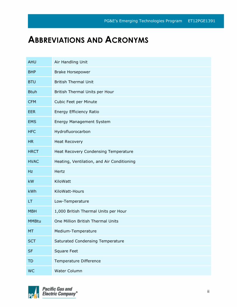
ABBREVIATIONS AND ACRONYMS

AHU Air Handling Unit

BHP Brake Horsepower

BTU British Thermal Unit

Btuh British Thermal Units per Hour

CFM Cubic Feet per Minute

EER Energy Efficiency Ratio

EMS Energy Management System

HFC Hydrofluorocarbon

HR Heat Recovery

HRCT Heat Recovery Condensing Temperature

HVAC Heating, Ventilation, and Air Conditioning

Hz Hertz

kW KiloWatt

kWh KiloWatt-Hours

LT Low-Temperature

MBH 1,000 British Thermal Units per Hour

MMBtu One Million British Thermal Units

MT Medium-Temperature

SCT Saturated Condensing Temperature

SF Square Feet

TD Temperature Difference

WC Water Column

iii


TABLE OF FIGURES Figure 1: Schematic Drawing of Heat Recovery System ..................... 5

Figure 2: Instrumentation Diagram for Heat Recovery Evaluation ....... 6

Figure 3: Heat Recovered and Consequent Natural Gas Savings Per

Month ......................................................................... 7

Figure 4: Electric Energy Usage for AHU Supply Fan, Compressors,

and Condenser Fans Per Month ...................................... 9

Figure 5: Net Energy Penalty Per Component for Full Test Period ..... 10

Figure 6: Holdback SCT and Mixed Return/Outside Air Temperature

for One Recovery System for 48 Hour Sample Period ...... 13

Figure 7: Pressure Drop across Holdback Valve and Valve Position

for One Sample Week ................................................. 14

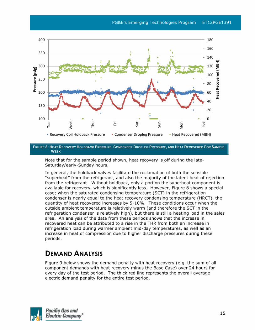
Figure 8: Heat Recovery Holdback Pressure, Condenser Dropleg

Pressure, and Heat Recovered For Sample Week ............ 15

Figure 9: Energy Penalty (Heat Recovery minus Base Case) for 24-

hour periods .............................................................. 16

Figure 10: Electric Demand by Component for Sample 24-Hour

Period ....................................................................... 16

Figure 11: Ambient Drybulb Temperature for Subject Test Period

from Actual Data and DOE-2.2R Analysis....................... 18

Figure 12: Bin Analysis of Ambient Drybulb Temperature from Test

Data and DOE-2.2R Simulation .................................... 18

Figure 13: Base Case Heating Fuel Usage for Main Sales Air

Handling Unit from DOE-2.2R Simulation and Observed

during Test Period ...................................................... 19

Figure 14: Heating Fuel Usage with Heat Recovery for Main Sales

Air Handling Unit from DOE-2.2R Simulation and

Observed during Test Period ........................................ 20

Figure 15: Refrigeration Load From Doe-2.2r Energy Model And

From Test Data .......................................................... 21

Figure 16: Total Refrigeration Load for Subject Test Period from

DOE-2.2R Energy Model and from Test Data .................. 22

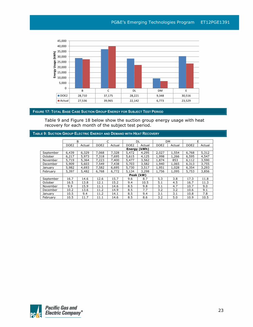
Figure 17: Total Base Case Suction Group Energy for Subject Test

Period ....................................................................... 23

Figure 18: Total Suction Group Energy with Heat Recovery for

Subject Test Period .................................................... 24

Figure 19: Net Electric Suction Group Energy Penalty from DOE-

2.2R Energy Model and from Test Data ......................... 24

Figure 20: Base Case Condenser Fan Energy for Subject Test

Period from DOE2 Analysis and from Test Data .............. 25

iv


Figure 21: Total Condenser Fan Energy with Heat Recovery for

Subject Test Period .................................................... 26

Figure 22: Difference in Base Case Condenser Fan Energy versus

with Heat Recovery .................................................... 27

Figure 23: AHU Supply Fan Energy for Subject Test Period from

DOE2 Analysis and Calculated from Actual Data ............. 28

Figure 24: VaCom Panel Simple Wiring Schematic .......................... 35

Figure 25: Schematic Drawing of Air Handling Unit, Showing 4-

Circuit Heat Recovery Coil ........................................... 38

Figure 26: Graph of Condenser Capacity and Condenser Power

versus Fan Speed ....................................................... 40

Figure 27: Flowchart of Calculations ............................................. 42

Figure 28: Typical Daily Fan Power Profiles For The Seasons4 Air

Handling Unit Supply Fan ............................................ 49

Figure 29: Average Hourly Heat Recovery Condensing Temperature

(Hrct) For Each Month................................................. 51

Figure 30: Natural Gas Usage History By Month, With And Without

Heat Recovery ........................................................... 53

Figure 31: Breakdown Of Natural Gas End-Use By Month Without

Heat Recovery ........................................................... 54

Figure 32: Breakdown Of Natural Gas End-Use By Month With Heat

Recovery ................................................................... 55

Figure 33: Electric Energy Usage By Month, With And Without Heat

Recovery ................................................................... 56

Figure 34: load profiles for Santa Clara County protocol b, shown

with comparable loads from The san diego and

encinitas Stores. ........................................................ 59

Figure 35: Load profiles for Santa Clara Store Protocol C, shown

with comparable loads from the San Diego and

Encinitas Stores ......................................................... 60

Figure 36: Load Profiles For Santa Clara County Protocol DL, Shown

With Comparable Loads From the San Diego And

Encinitas Stores ......................................................... 60

Figure 37: Load Profiles For Santa Clara County Protocol DM,

Shown With Comparable Loads From The San Diego

And Encinitas Stores .................................................. 60

Figure 38: Load Profiles For Santa Clara County Protocol E, Shown

With Comparable Loads From San Diego and Encinitas

Stores ....................................................................... 61

Figure 39: Natural Gas Usage For the Santa Clara County Store,

Compared To Two Other Supermarkets ......................... 62

v


TABLE OF TABLES Table 1: Heat Recovery Evaluation Results Summary ........................ 2

Table 2: Main AHU Supply Fan Static Pressure, Power, and Energy

Usage ......................................................................... 8

Table 3: Summary of E-19 Electric Energy Schedule ....................... 10

Table 4: Summary of G-NR1 Natural Gas Schedule ......................... 11

Table 5: Electric Energy and Demand Cost, and Natural Gas Cost,

for the Test Period ...................................................... 11

Table 6: Hours with Ambient DBT Below 65°F: Actual Data vs.

DOE-2.2R Simulation .................................................. 19

Table 7: Refrigeration Load from DOE-2.2R Energy Model and from

Test Data .................................................................. 21

Table 8: Base Case Suction Group Electric Energy and Demand ....... 22

Table 9: Suction Group Electric Energy and Demand with Heat

Recovery ................................................................... 23

Table 10: Base Case Condenser Fan Energy for Subject Test Period

from DOE2 Analysis and from Test Data ........................ 25

Table 11: Condenser Fan Energy with Heat Recovery for Subject

Test Period from DOE2 Analysis and from Test Data ....... 26

Table 12: AHU Supply Fan Electric Energy Usage from DOE2

Analysis and Calculated from Actual data ...................... 27

Table 13: Calculated Charge Increase for Subject Heat Recovery

System ..................................................................... 30

Table 14: Calculated Charge Increase for Subject Heat Recovery

System with Low-Charge Condensers ........................... 31

Table 15: R-507A Refrigerant Charge Per System in Pounds ............ 31

Table 16: Heat Recovery Project Cost Estimate .............................. 32

Table 17: Simple Payback, Net Present Value, and Internal Rate of

Return Analysis without Incentives ............................... 32

Table 18: Simple Payback, Net Present Value, and Internal Rate of

Return Analysis with Incentives .................................... 32

Table 19: Sensors Added for the Field Study .................................. 34

Table 20: .csv File Format ........................................................... 36

Table 21: Instrumentation Connected to Danfoss EMS System ......... 37

Table 22: Condenser Part-Load Performance from Laboratory

Testing ..................................................................... 40

Table 23: Air Handling Unit Properties .......................................... 48

Table 24: Heat Recovery Coil Parameters ...................................... 48

vi


Table 25: Heat Recovery Coil Capacity .......................................... 49

Table 26: PG&E E-19V Energy Tarriff ............................................ 51

Table 27: DOE2 Simulation Results............................................... 52

Table 28: Whole-Building Peak Demand By Month, With And

Without Heat Recovery ............................................... 57

Table 29: refrigeration loads from stores that were monitoried ........ 58

Table 30: Envelope Description .................................................... 63

Table 31: Lighting Power ............................................................. 63

Table 32: Hussmann Protocol Refrigeration System Summary ......... 64

Table 33: Krack LAVE Condenser Summary ................................... 65

Table 34: Open Case Summary .................................................... 66

Table 35: Open Case LED Light Summary ..................................... 67

Table 36: Door Case Summary .................................................... 67

Table 37: Summary Of Assumed Background Loads Per Space ........ 68

Table 38: Abbreviated List Of Loads For The Bakery Space .............. 68

Table 39: Assumed Background Natural Gas Loads ......................... 69

vii


TABLE OF CONTENTS

ABBREVIATIONS AND ACRONYMS _____________________________________________ II

TABLE OF FIGURES ________________________________________________________ III

TABLE OF TABLES _________________________________________________________ V

TABLE OF CONTENTS ______________________________________________________VII

EXECUTIVE SUMMARY _____________________________________________________ 1

HISTORY _______________________________________________________________ 4

ASSESSMENT OBJECTIVES __________________________________________________ 4

TECHNOLOGY EVALUATION ________________________________________________ 4

TEST METHODOLOGY _____________________________________________________ 6

RESULTS________________________________________________________________ 6

Natural Gas Usage and Savings................................................. 7

Electric Energy Usage and Penalty ............................................. 7

AHU Supply Fan Energy ...................................................... 7

Condenser Fan Energy ........................................................ 8

Compressor Energy ............................................................ 8

Electric Energy Usage and Penalty Results ............................. 9

Cost Results ......................................................................... 10

ANALYSIS _____________________________________________________________ 12

Holdback valve Operation ....................................................... 12

Valve Control and Pressure Drop Analysis ............................ 13

Demand Analysis .................................................................. 15

Loads and Energy Usage versus DOE2 Analysis ......................... 17

Comparison of Ambient Temperature Data .......................... 17

Refrigeration System Performance ..................................... 20

AHU Supply Fan Energy .................................................... 27

Heat Recovered versus Whole Building THR ......................... 29

Refrigerant Charge Analysis ............................................... 29

Economics Analysis ............................................................... 31

CONCLUSIONS _________________________________________________________ 33

APPENDIX A: ANALYSIS PLAN______________________________________________ 34

Instrumentation .................................................................... 34

viii


Danfoss EMS System Instrumentation ..................................... 36

Analysis Plan ........................................................................ 37

Pre-Installation Instrumentation commissioning ................... 37

Instrumentation Field Commissioning ................................. 37

Static Pressure Drop across Air Handling Unit Components: ... 38

Airflow Symmetry across Heat Recovery Coil Circuits: ........... 38

Amperage Draw and Power Factors: ................................... 38

Data Collection ................................................................ 39

Measuring Heat Recovery Performance ............................... 39

Establishing Base Case Performance ................................... 39

Calculations Summary ...................................................... 42

Calculations for Therm Savings .......................................... 42

Calculations for Net Electric Energy Penalty ......................... 43

APPENDIX B: DOE-2.2R SIMULATION _______________________________________ 48

Heat Recovery System Description .......................................... 48

Air Handling Unit and Heat Recovery Control ............................ 48

Supply Fan Control ................................................................ 49

Holdback Valve Control .......................................................... 50

Outside Air ........................................................................... 51

Energy Costs ........................................................................ 51

Results ................................................................................ 52

Natural Gas Usage ............................................................ 52

Electrical Energy Usage ..................................................... 55

Condenser Efficiency Considerations ................................... 57

Model Calibration and Validation ............................................. 57

Field Testing of Technology ............................................... 57

Natural Gas Usage Analysis ............................................... 61

APPENDIX C: BUILDING SUMMARY __________________________________________ 63

Envelope and Lighting Power .................................................. 63

Hussmann Protocol Refrigeration Systems ................................ 64

Krack Air-Cooled Condensers .................................................. 64

Refrigerated Display Cases and Walk-Ins ................................. 65

Refrigerated Display Cases and Walk-Ins ................................. 67

Electric Energy ...................................................................... 67

Natural Gas .......................................................................... 69

1


EXECUTIVE SUMMARY Pacific Gas & Electric Company (PG&E) worked with a retail grocery store chain to study

heat recovery in a new supermarket in Santa Clara County, California. Energy analysis and

field monitoring were conducted to better understand the natural gas savings and

consequent electric energy penalty associated with a heat recovery system using the heat

from the market’s refrigeration systems to heat the sales area. PG&E assisted the

Customer and its controls and equipment vendors during the design and construction phase

of the new supermarket to evaluate multiple design options, configure the recovery system,

size and select the heat exchanger and holdback valves, and prepare control sequences of

operation for the heat recovery controls. PG&E also assisted during start-up and

commissioning phases.

PROJECT DESCRIPTION

The subject system is a direct-condensing system using heat from four of the store’s six

distributed refrigeration systems, with the four systems rejecting heat via a four-circuit

parallel refrigerant-to-air heat exchanger coil in the main air handling unit that serves the

store’s sales area. Electronic pressure regulating “holdback” valves at the outlet of the heat

exchanger facilitate both sensible and latent heat exchange—significantly increasing the

quantity of heat recovered (versus systems without holdback valves, where only a portion

of the latent heat is available), with a consequent increase in compressor discharge

pressures and consumed compressor energy (which is typical for systems with holdback

pressure control, but is less than the resulting heating energy and cost savings).

The performance of the heat recovery system was evaluated versus a theoretical Base Case

system consisting of the same refrigeration and HVAC systems operating with the same

ambient conditions, refrigeration loads, and heating loads as the system with heat recovery,

but absent of all of the components related to heat recovery. The Base Case system

performance was calculated analytically.

The refrigeration systems and air handling unit were outfitted with instrumentation and data

acquisition equipment to monitor electric energy and natural gas usage. An on-site

monitoring panel collected the sensor data and transmitted it for processing via wireless

modem. The instrumentation included sensors to monitor the refrigerant pressure and

temperature inside and downstream of the recovery coil, air temperature entering and

leaving each recovery coil circuit, air flowrate, and natural gas flowrate. The store’s

Danfoss energy management system (EMS) was also used to obtain additional refrigeration

system data for the compressors, condensers, and other system operating parameters.

Several challenges were encountered, including:

Complications with incorporating the holdback valves into the heat recovery design.

Contractors, controls vendors, and equipment vendors hesitated to use the valves,

instead opting to use the less sophisticated (and lower performing) design without

holdback pressure control. PG&E worked closely with the vendors and contractors to

incorporate the holdback valves and pump-out circuits into the construction

drawings, properly size the coil and valves, and to develop functional descriptions of

the valve control sequences.

2


Delays in the construction schedule, related to changes in the store’s corporate

ownership as well as post-construction store design changes. The store was

originally scheduled to open on October 18, 2013, but the grand opening did not

occur until May 2, 2014. Final commissioning of the heat recovery systems was not

complete until August, 2014. In response, the monitoring phase of this Emerging

Technologies study was shortened from 12 months to 6 months.

Issues with automatic data transfer from the Danfoss EMS system, requiring close

cooperation between PG&E, Danfoss, and the Customer’s IT department, and

multiple software revisions by Danfoss to its StoreView remote access software.

Instrument failures that occurred during the construction and monitoring phase,

notably the supply air flowrate meter (installed during the construction phase, the

pressure lines from the pitot arrays were disconnected from the

transducer/transmitter when the ceiling tiles were hung), and the natural gas flow

meter (the original diaphragm-style meters were destroyed by natural gas inrush.

After two diaphragm-style meters failed, a more robust rotary-style meter was used

instead. Neither PG&E or the meter vendor had experience with this failure mode

before).

The heat recovery system was fully commissioned in August, 2014. The dataset for this

analysis starts on September 1, 2014, and ends on February 28, 2015.

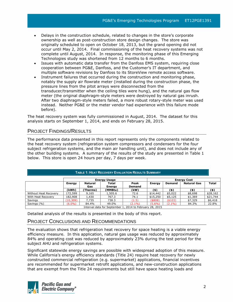
PROJECT FINDINGS/RESULTS

The performance data presented in this report represents only the components related to

the heat recovery system (refrigeration system compressors and condensers for the four

subject refrigeration systems, and the main air handling unit), and does not include any of

the other building systems. A summary of the results of the study are presented in Table 1

below. This store is open 24 hours per day, 7 days per week.

TABLE 1: HEAT RECOVERY EVALUATION RESULTS SUMMARY

Energy Usage Energy Cost

Energy Natural

Gas

Total

Energy

Peak

Demand

Energy Demand Natural Gas Total

(kWh) (Therms) (MMBtu) (kW) ($) ($) ($) ($)

Without Heat Recovery 172,599 9,165 1,505.6 72.6 $14,442 $5,022 $8,698 $28,162

With Heat Recovery 182,908 1,430 767.3 74.1 $15,250 $5,125 $1,369 $21,744

Savings (10,309) 7,735 738.3 (1.5) ($808) ($103) $7,329 $6,418

Savings (%) (6.0%) 84.4% 49.0% (2.1%) (5.6%) (2.1%) 84.3% 22.8%

Interval data for September 1, 2014 to February 28, 2015

Detailed analysis of the results is presented in the body of this report.

PROJECT CONCLUSIONS AND RECOMMENDATIONS

The evaluation shows that refrigeration heat recovery for space heating is a viable energy

efficiency measure. In this application, natural gas usage was reduced by approximately

84% and operating cost was reduced by approximately 23% during the test period for the

subject AHU and refrigeration systems.

Significant statewide energy savings are possible with widespread adoption of this measure.

While California’s energy efficiency standards (Title 24) require heat recovery for newly

constructed commercial refrigeration (e.g. supermarket) applications, financial incentives

are recommended for supermarket retrofit applications, and new-construction applications

that are exempt from the Title 24 requirements but still have space heating loads and

3


refrigeration capacity. However, substantial market support and training by the California

utility companies (beyond just incentives) is needed to achieve the intended savings levels

and market penetration, while balancing electric energy penalty and refrigerant charge

increase. Specifically, the industry seems to have lost much of the technical understanding

related to holdback valve utilization and control.

The focus of this project was a direct-condensing heat recovery system, where heat is

exchanged from refrigerant directly to air. Other heat recovery configurations are viable,

with comparable (or even higher) savings expectations, which would be more suitable for

retrofit applications. One configuration in particular is the indirect design, where recovered

heat is transferred from the refrigerant to an intermediate fluid (normally water or water-

glycol) which is circulated through a fluid-to-air heat exchanger located in the air handling

unit airstream.

4


HISTORY Use of heat from refrigeration systems to provide space heating in supermarkets has a long

history and at one time was used extensively and provided all or most of the heat in many

stores, both in California and across the US. However, heat recovery became less common

in recent decades, largely because of the perception that heat recovery systems significantly

increase refrigerant charge and leakage. Many supermarket chains are again considering

low-charge heat recovery systems as a way to reduce natural gas usage and operating

costs, and in order to meet sustainability objectives. In addition, the 2013 California Title

24 Building Energy Efficiency Standards include requirements for heat recovery systems in

new-construction projects. Title 24 mandates that at least 25% of the heat of rejection

(THR) from refrigeration systems shall be used for space heating in new supermarkets.

ASSESSMENT OBJECTIVES This project assessed the natural gas energy savings from a direct-condensing refrigerant-

to-air heat recovery system for space heating in a supermarket in Santa Clara County,

California. The project compared the performance of the heat recovery system to a “Base

Case” system with no refrigeration heat recovery, a standard natural-gas furnace for space

heating, and typical distributed single-stage R-507A parallel commercial refrigeration

systems.

This project provides the necessary instrumentation, data acquisition equipment, and

analysis required to monitor and evaluate the electric energy and natural gas usage of the

refrigeration systems and air handling unit. The data was processed and compared to a

theoretical scenario consisting of refrigeration and HVAC systems with no connected heat

recovery capacity.

TECHNOLOGY EVALUATION The subject heat recovery system consists of a four-circuit direct-condensing heat recovery

coil installed inside the main air handling unit (AHU) that serves the supermarket’s main

sales area. Within the AHU, the coil is located upstream of the natural gas furnace, with

each coil circuit connected to the discharge of one of four refrigeration systems

(designations B, C, D, and E). The heat recovery coil is connected in series with the air-

cooled refrigeration condensers for each refrigeration system. Three-way control valves

divert refrigerant from the refrigeration compressors to the heat recovery coil and then to

the refrigeration condensers when the system is in heat recovery mode. When the system

is not in heat recovery mode, the three-way valve diverts refrigerant directly to the

refrigeration condensers. Because the system is designed to operate with or without the

reclaim activated, the sizing and specification of the condensers is equivalent to a design

without reclaim. Pump-out circuits are included to evacuate the heat recovery coils to the

refrigeration suction header when the system is not in heat recovery mode.

5


Four electronic holdback valves located immediately downstream of each of the heat

recovery coil circuits control the refrigerant pressure inside the coil. Holding the refrigerant

inside the coil at a higher pressure induces condensation of the refrigerant from a vapor

state to mostly liquid, recovering much of the latent heat that would otherwise not be

available without holdback valves. The valves are controlled so that the temperature

difference (TD) between the mixed return/outside air and the refrigerant condensing

temperature inside the heat recovery coil is held constant (subject to programmed

maximum and minimum condensing temperatures). Figure 1 below is a schematic drawing

of a refrigeration heat recovery system. For simplicity, only one of four circuits is shown.

FIGURE 1: SCHEMATIC DRAWING OF HEAT RECOVERY SYSTEM

Heat recovery is the primary source for space heating. The AHU natural gas furnace is used

only when heat recovery from all four refrigeration systems are already active and

additional heating capacity is required. Staging of this process consists of:

Stage 1: Heat recovery from Refrigeration Systems B and C

Stage 2: Includes Stage 1, and adds the heat recovery from Refrigeration Systems D

and E

Stage 3: Includes Stages 1 and 2, and adds the AHU natural gas furnace

6


TEST METHODOLOGY Pressure and temperature sensors were added to the four subject refrigeration systems.

Airflow, natural gas flow, and air temperature sensors were added to the air handling unit

where the heat recovery condensing coil is installed. A monitoring panel located in the

condenser section of the air handling unit collected the sensor data and transmitted it for

processing via wireless modem. The store’s Danfoss energy management system was also

used to obtain additional refrigeration system data for the compressors, condensers, air

handling unit, space temperature and relative humidity, outside ambient temperature, and

other system operating parameters.

FIGURE 2: INSTRUMENTATION DIAGRAM FOR HEAT RECOVERY EVALUATION

For a detailed description of the evaluation methodology, refer to Appendix A: Analysis Plan.

RESULTS

Presented below are the results for the heat recovery ET project. The recovery system is

expected to save gas that would have been used in the furnace to heat the supply air, while

using more electricity because of an increase in load on the AHU fan and an elevated energy

usage in the refrigeration. The results are presented in the following sections:

Natural Gas Usage and Savings

Electric Energy Usage and Penalty

Cost Results

The dataset for this analysis starts on September 1, 2014, and ends on February 28, 2015

7


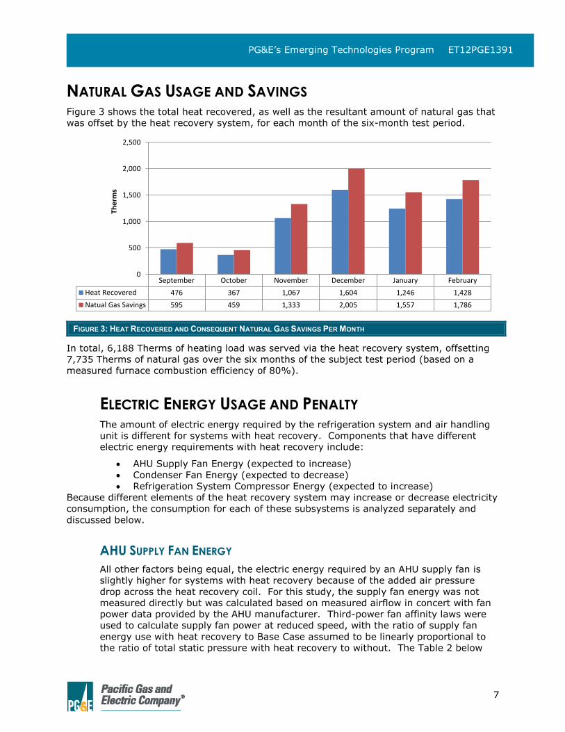
NATURAL GAS USAGE AND SAVINGS Figure 3 shows the total heat recovered, as well as the resultant amount of natural gas that

was offset by the heat recovery system, for each month of the six-month test period.

FIGURE 3: HEAT RECOVERED AND CONSEQUENT NATURAL GAS SAVINGS PER MONTH

In total, 6,188 Therms of heating load was served via the heat recovery system, offsetting

7,735 Therms of natural gas over the six months of the subject test period (based on a

measured furnace combustion efficiency of 80%).

ELECTRIC ENERGY USAGE AND PENALTY The amount of electric energy required by the refrigeration system and air handling

unit is different for systems with heat recovery. Components that have different

electric energy requirements with heat recovery include:

AHU Supply Fan Energy (expected to increase)

Condenser Fan Energy (expected to decrease)

Refrigeration System Compressor Energy (expected to increase)

Because different elements of the heat recovery system may increase or decrease electricity

consumption, the consumption for each of these subsystems is analyzed separately and

discussed below.

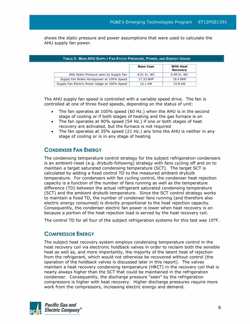
AHU SUPPLY FAN ENERGY

All other factors being equal, the electric energy required by an AHU supply fan is

slightly higher for systems with heat recovery because of the added air pressure

drop across the heat recovery coil. For this study, the supply fan energy was not

measured directly but was calculated based on measured airflow in concert with fan

power data provided by the AHU manufacturer. Third-power fan affinity laws were

used to calculate supply fan power at reduced speed, with the ratio of supply fan

energy use with heat recovery to Base Case assumed to be linearly proportional to

the ratio of total static pressure with heat recovery to without. The Table 2 below

September October November December January February

Heat Recovered 476 367 1,067 1,604 1,246 1,428

Natual Gas Savings 595 459 1,333 2,005 1,557 1,786

0

500

1,000

1,500

2,000

2,500

The

rms

8


shows the static pressure and power assumptions that were used to calculate the

AHU supply fan power.

TABLE 2: MAIN AHU SUPPLY FAN STATIC PRESSURE, POWER, AND ENERGY USAGE

Base Case With Heat

Recovery

AHU Static Pressure seen by Supply Fan 4.01 In. WC 4.49 In. WC

Supply Fan Brake Horsepower at 100% Speed 17.33 BHP 19.4 BHP

Supply Fan Electric Power Usage at 100% Speed 14.1 kW 15.8 kW

The AHU supply fan speed is controlled with a variable speed drive. The fan is

controlled at one of three fixed speeds, depending on the status of unit:

The fan operates at 100% speed (60 Hz.) when the AHU is in the second

stage of cooling or if both stages of heating and the gas furnace is on

The fan operates at 90% speed (54 Hz.) if one or both stages of heat

recovery are activated, but the furnace is not required

The fan operates at 35% speed (21 Hz.) any time the AHU is neither in any

stage of cooling or is in any stage of heating

CONDENSER FAN ENERGY

The condensing temperature control strategy for the subject refrigeration condensers

is an ambient-reset (e.g. drybulb-following) strategy with fans cycling off and on to

maintain a target saturated condensing temperature (SCT). The target SCT is

calculated by adding a fixed control TD to the measured ambient drybulb

temperature. For condensers with fan cycling control, the condenser heat rejection

capacity is a function of the number of fans running as well as the temperature

difference (TD) between the actual refrigerant saturated condensing temperature

(SCT) and the ambient drybulb temperature. Since the SCT control strategy works

to maintain a fixed TD, the number of condenser fans running (and therefore also

electric energy consumed) is directly proportional to the heat rejection capacity.

Consequently, the condenser electric fan power is lower when heat recovery is on

because a portion of the heat rejection load is served by the heat recovery coil.

The control TD for all four of the subject refrigeration systems for this test was 10°F.

COMPRESSOR ENERGY

The subject heat recovery system employs condensing temperature control in the

heat recovery coil via electronic holdback valves in order to reclaim both the sensible

heat as well as, and more importantly, the majority of the latent heat of rejection

from the refrigerant, which would not otherwise be recovered without control (the

operation of the holdback valves is discussed later in this report). The valves

maintain a heat recovery condensing temperature (HRCT) in the recovery coil that is

nearly always higher than the SCT that could be maintained in the refrigeration

condenser. Consequently, the discharge pressure “seen” by the refrigeration

compressors is higher with heat recovery. Higher discharge pressures require more

work from the compressors, increasing electric energy and demand.

9


ELECTRIC ENERGY USAGE AND PENALTY RESULTS

Figure 4 illustrates the calculated electric energy use by month for the refrigeration

system compressors and condensers, and for the air handling unit supply fan. The

electric energy use was calculated based on performance data provided by the

component manufacturer, and measured capacity and run-times from the test data.

The top figure shows the calculated Base Case energy usage, while the bottom figure

shows the energy usage with the heat recovery system.

FIGURE 4: ELECTRIC ENERGY USAGE FOR AHU SUPPLY FAN, COMPRESSORS, AND CONDENSER FANS PER MONTH

Figure 5 below shows the total energy penalty (calculated as energy usage with heat

recovery minus Base Case energy usage) for the entire test period, for each of the

components analyzed in this study.


Base Case Supply Fan 3,389 3,260 4,660 9,173 6,977 5,081

Base Case Condensers 3,959 3,581 2,711 3,555 2,782 2,371

Base Case Compressors 25,823 22,517 17,398 22,514 17,924 14,959

0

10,000

20,000

30,000

40,000

50,000

60,000

Ene

rgy

(kW

h)


Supply Fan with HR 3,795 3,650 5,218 10,271 7,812 5,689

Condenser with HR 3,528 3,349 1,942 2,178 2,454 1,421

Compressors with HR 26,530 23,384 19,407 26,010 19,246 17,063

0

10,000

20,000

30,000

40,000

50,000

60,000

Ene

rgy

(kW

h)

10


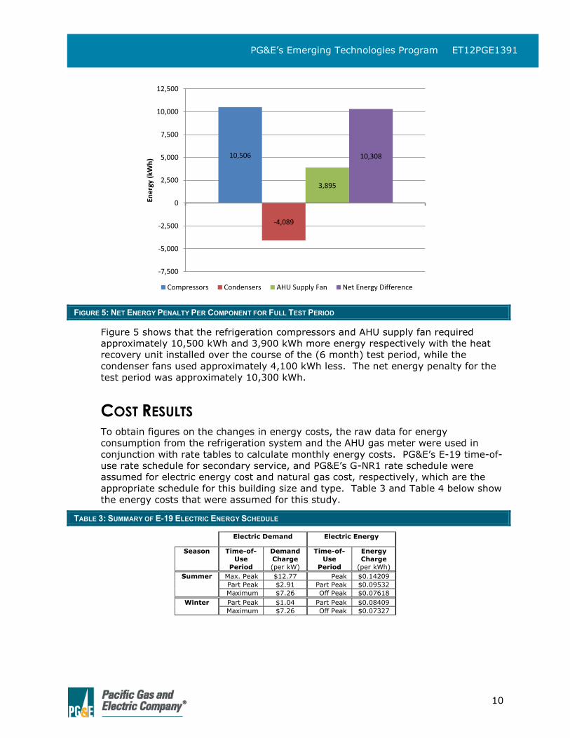
FIGURE 5: NET ENERGY PENALTY PER COMPONENT FOR FULL TEST PERIOD

Figure 5 shows that the refrigeration compressors and AHU supply fan required

approximately 10,500 kWh and 3,900 kWh more energy respectively with the heat

recovery unit installed over the course of the (6 month) test period, while the

condenser fans used approximately 4,100 kWh less. The net energy penalty for the

test period was approximately 10,300 kWh.

COST RESULTS To obtain figures on the changes in energy costs, the raw data for energy

consumption from the refrigeration system and the AHU gas meter were used in

conjunction with rate tables to calculate monthly energy costs. PG&E’s E-19 time-of-

use rate schedule for secondary service, and PG&E’s G-NR1 rate schedule were

assumed for electric energy cost and natural gas cost, respectively, which are the

appropriate schedule for this building size and type. Table 3 and Table 4 below show

the energy costs that were assumed for this study.

TABLE 3: SUMMARY OF E-19 ELECTRIC ENERGY SCHEDULE

Electric Demand Electric Energy

Season Time-of-

Use

Period

Demand

Charge

(per kW)

Time-of-

Use

Period

Energy

Charge

(per kWh)

Summer Max. Peak $12.77 Peak $0.14209

Part Peak $2.91 Part Peak $0.09532

Maximum $7.26 Off Peak $0.07618

Winter Part Peak $1.04 Part Peak $0.08409

Maximum $7.26 Off Peak $0.07327

10,506

-4,089

3,895

10,308

-7,500

-5,000

-2,500

0

2,500

5,000

7,500

10,000

12,500

Ene

rgy

(kW

h)

Compressors Condensers AHU Supply Fan Net Energy Difference

11


TABLE 4: SUMMARY OF G-NR1 NATURAL GAS SCHEDULE

Summer Winter

First 4,000 Therms Excess Therms First 4,000 Therms Excess Therms

Procurement $0.56306 $0.56306 $0.56306 $0.56306

Transportation $0.32278 $0.16637 $0.39418 $0.20318

Total Charge $0.88584 $0.72943 $0.95724 $0.76624

Table 5 below summarizes the electric energy, electric demand, and natural gas cost

by month, as well as the aggregate cost results for the test period.

TABLE 5: ELECTRIC ENERGY AND DEMAND COST, AND NATURAL GAS COST, FOR THE TEST PERIOD

Base Case With Heat Recovery Difference

Month

Energy

Cost ($)

Demand

Cost ($)

Total

Energy

Cost ($)

Energy

Cost ($)

Demand

Cost ($)

Total

Energy

Cost ($)

Energy

Cost ($)

Demand

Cost ($)

Total

Energy

Cost ($)

September $2,964 $1,650 $4,615 $3,019 $1,686 $4,704 $54 $35 $90

October $2,842 $1,535 $4,376 $2,934 $1,570 $4,505 $93 $35 $128

November $2,080 $439 $2,519 $2,229 $449 $2,678 $149 $10 $159

December $2,283 $467 $2,750 $2,490 $472 $2,962 $207 $5 $212

January $2,168 $451 $2,618 $2,309 $465 $2,774 $141 $15 $156

February $2,105 $480 $2,585 $2,269 $483 $2,753 $164 $3 $167

TOTAL $14,442 $5,022 $19,463 $15,250 $5,125 $20,376 $809 $104 $912

Natural Gas Usage (Therms) Cost ($)

Month Base Case

With Heat

Recovery Base Case

With Heat

Recovery Savings

September 595 0 $527 $0 $527

October 459 0 $407 $0 $407

November 2,061 728 $1,973 $697 $1,276

December 2,005 0 $1,919 $0 $1,919

January 1,658 101 $1,587 $97 $1,490

February 2,387 602 $2,285 $576 $1,709

Total: 9,165 1,430 $8,698 $1,369 $7,329

Energy Cost

Energy Demand Total Electric Energy Natural Gas Total

($) ($) ($) ($) ($)

Without Heat Recovery $14,442 $5,022 $19,464 $8,698 $28,162

With Heat Recovery $15,250 $5,125 $20,375 $1,369 $21,744

Savings ($808) ($103) ($911) $7,329 $6,418

Savings (%) (5.6%) (2.1%) (4.7%) 84.3% 22.8%

Table 5 shows that heat recovery offset $7,300, or 84%, of natural gas cost for heating

energy. The consequent increase in electric energy and demand cost was $911, or 5%.

Overall, the heat recovery system saved approximately $6,400, or 23% of the total energy

cost for these 6 months.

12


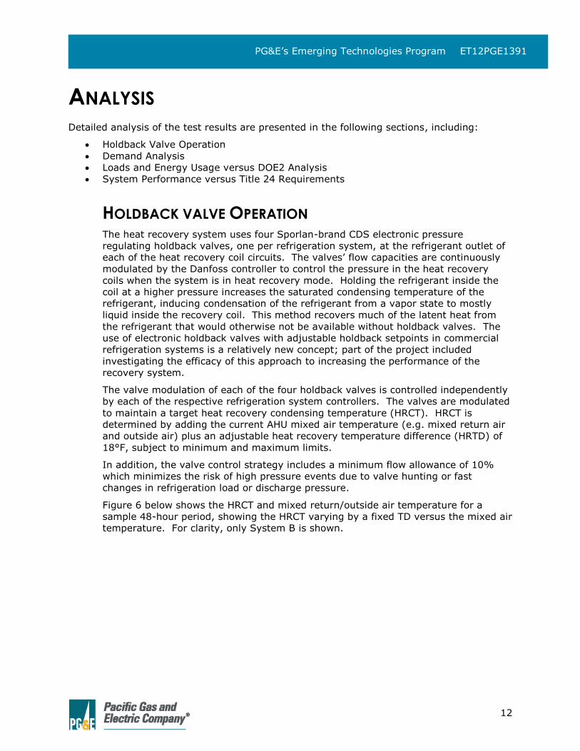
ANALYSIS Detailed analysis of the test results are presented in the following sections, including:

Holdback Valve Operation

Demand Analysis

Loads and Energy Usage versus DOE2 Analysis

System Performance versus Title 24 Requirements

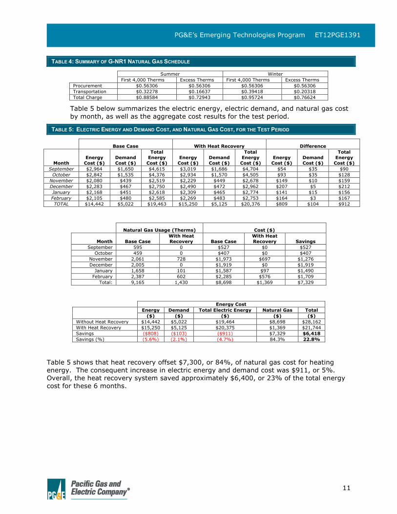
HOLDBACK VALVE OPERATION The heat recovery system uses four Sporlan-brand CDS electronic pressure

regulating holdback valves, one per refrigeration system, at the refrigerant outlet of

each of the heat recovery coil circuits. The valves’ flow capacities are continuously

modulated by the Danfoss controller to control the pressure in the heat recovery

coils when the system is in heat recovery mode. Holding the refrigerant inside the

coil at a higher pressure increases the saturated condensing temperature of the

refrigerant, inducing condensation of the refrigerant from a vapor state to mostly

liquid inside the recovery coil. This method recovers much of the latent heat from

the refrigerant that would otherwise not be available without holdback valves. The

use of electronic holdback valves with adjustable holdback setpoints in commercial

refrigeration systems is a relatively new concept; part of the project included

investigating the efficacy of this approach to increasing the performance of the

recovery system.

The valve modulation of each of the four holdback valves is controlled independently

by each of the respective refrigeration system controllers. The valves are modulated

to maintain a target heat recovery condensing temperature (HRCT). HRCT is

determined by adding the current AHU mixed air temperature (e.g. mixed return air

and outside air) plus an adjustable heat recovery temperature difference (HRTD) of

18°F, subject to minimum and maximum limits.

In addition, the valve control strategy includes a minimum flow allowance of 10%

which minimizes the risk of high pressure events due to valve hunting or fast

changes in refrigeration load or discharge pressure.

Figure 6 below shows the HRCT and mixed return/outside air temperature for a

sample 48-hour period, showing the HRCT varying by a fixed TD versus the mixed air

temperature. For clarity, only System B is shown.

13


FIGURE 6: HOLDBACK SCT AND MIXED RETURN/OUTSIDE AIR TEMPERATURE FOR ONE RECOVERY SYSTEM FOR 48 HOUR

SAMPLE PERIOD

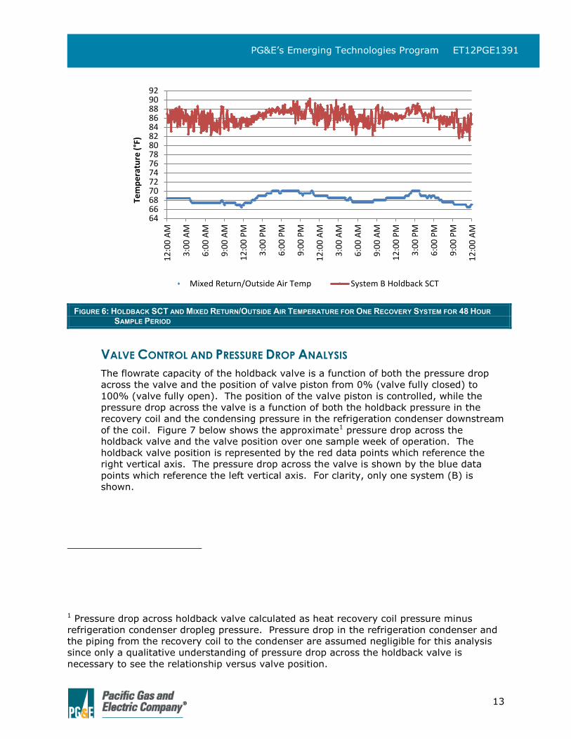
VALVE CONTROL AND PRESSURE DROP ANALYSIS

The flowrate capacity of the holdback valve is a function of both the pressure drop

across the valve and the position of valve piston from 0% (valve fully closed) to

100% (valve fully open). The position of the valve piston is controlled, while the

pressure drop across the valve is a function of both the holdback pressure in the

recovery coil and the condensing pressure in the refrigeration condenser downstream

of the coil. Figure 7 below shows the approximate1 pressure drop across the

holdback valve and the valve position over one sample week of operation. The

holdback valve position is represented by the red data points which reference the

right vertical axis. The pressure drop across the valve is shown by the blue data

points which reference the left vertical axis. For clarity, only one system (B) is

shown.

1 Pressure drop across holdback valve calculated as heat recovery coil pressure minus

refrigeration condenser dropleg pressure. Pressure drop in the refrigeration condenser and

the piping from the recovery coil to the condenser are assumed negligible for this analysis

since only a qualitative understanding of pressure drop across the holdback valve is

necessary to see the relationship versus valve position.

646668707274767880828486889092

12

:00

AM

3:0

0 A

M

6:0

0 A

M

9:0

0 A

M

12

:00

PM

3:0

0 P

M

6:0

0 P

M

9:0

0 P

M

12

:00

AM

3:0

0 A

M

6:0

0 A

M

9:0

0 A

M

12

:00

PM

3:0

0 P

M

6:0

0 P

M

9:0

0 P

M

12

:00

AM

Tem

pe

ratu

re (

°F)

Mixed Return/Outside Air Temp System B Holdback SCT

14


FIGURE 7: PRESSURE DROP ACROSS HOLDBACK VALVE AND VALVE POSITION FOR ONE SAMPLE WEEK

Figure 7 shows that the relationship between the valve position and the pressure

drop are inversely related; the valve is only partially open when pressure drop is

high, and is nearly (and at times fully) open when pressure drop is low, which

matches expectations.

The quantity of heat recovered for the same test period as above is shown in Figure

8. The heat recovery coil holdback pressure and condenser dropleg pressure are

shown in blue and red, respectively, and reference the left vertical axis, while the

heat recovered is shown in green and references the right vertical axis.

0%

20%

40%

60%

80%

100%

120%

140%

160%

180%

200%

0

10

20

30

40

50

60

70

80

Tue

We

d

Thu

Fri

Sat

Sun

Mo

n

Tue

Val

ve P

osi

tio

n (

% O

pe

n)

Pre

ssu

re d

rop

(p

si)

Pressure Drop across Heat Recovery Holdback Valve Holdback Valve % Open

15


FIGURE 8: HEAT RECOVERY HOLDBACK PRESSURE, CONDENSER DROPLEG PRESSURE, AND HEAT RECOVERED FOR SAMPLE

WEEK

Note that for the sample period shown, heat recovery is off during the late-

Saturday/early-Sunday hours.

In general, the holdback valves facilitate the reclamation of both the sensible

“superheat” from the refrigerant, and also the majority of the latent heat of rejection

from the refrigerant. Without holdback, only a portion the superheat component is

available for recovery, which is significantly less. However, Figure 8 shows a special

case; when the saturated condensing temperature (SCT) in the refrigeration

condenser is nearly equal to the heat recovery condensing temperature (HRCT), the

quantity of heat recovered increases by 5-10%. These conditions occur when the

outside ambient temperature is relatively warm (and therefore the SCT in the

refrigeration condenser is relatively high), but there is still a heating load in the sales

area. An analysis of the data from these periods shows that the increase in

recovered heat can be attributed to a rise in the THR from both an increase in

refrigeration load during warmer ambient mid-day temperatures, as well as an

increase in heat of compression due to higher discharge pressures during these

periods.

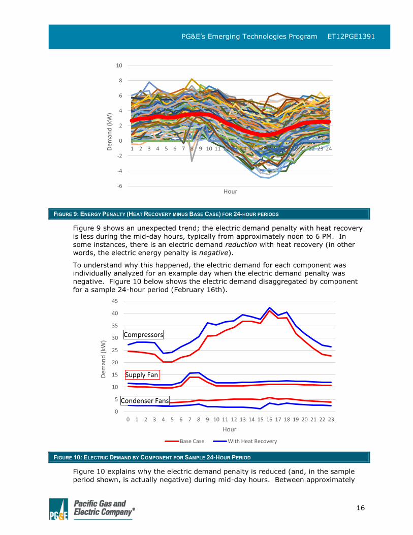
DEMAND ANALYSIS Figure 9 below shows the demand penalty with heat recovery (e.g. the sum of all

component demands with heat recovery minus the Base Case) over 24 hours for

every day of the test period. The thick red line represents the overall average

electric demand penalty for the entire test period.

0

20

40

60

80

100

120

140

160

180

100

150

200

250

300

350

400

Tue

We

d

Thu

Fri

Sat

Sun

Mo

n

Tue

He

at R

eco

vere

d (

MB

H)

Pre

ssu

re (

psi

g)

Recovery Coil Holdback Pressure Condenser Dropleg Pressure Heat Recovered (MBH)

16


FIGURE 9: ENERGY PENALTY (HEAT RECOVERY MINUS BASE CASE) FOR 24-HOUR PERIODS

Figure 9 shows an unexpected trend; the electric demand penalty with heat recovery

is less during the mid-day hours, typically from approximately noon to 6 PM. In

some instances, there is an electric demand reduction with heat recovery (in other

words, the electric energy penalty is negative).

To understand why this happened, the electric demand for each component was

individually analyzed for an example day when the electric demand penalty was

negative. Figure 10 below shows the electric demand disaggregated by component

for a sample 24-hour period (February 16th).

FIGURE 10: ELECTRIC DEMAND BY COMPONENT FOR SAMPLE 24-HOUR PERIOD

Figure 10 explains why the electric demand penalty is reduced (and, in the sample

period shown, is actually negative) during mid-day hours. Between approximately

-6

-4

-2

0

2

4

6

8

10

1 2 3 4 5 6 7 8 9 10 11 12 13 14 15 16 17 18 19 20 21 22 23 24Dem

and

(kW

)

Hour

0

5

10

15

20

25

30

35

40

45

0 1 2 3 4 5 6 7 8 9 10 11 12 13 14 15 16 17 18 19 20 21 22 23

Dem

and

(kW

)

Hour

Base Case With Heat Recovery

Compressors

Supply Fan

Condenser Fans

17


noon and six PM, the compressor demand with heat recovery is nearly equal to the

Base Case demand (e.g. near-zero penalty), and the condenser fan demand

reduction with heat recovery is larger than the demand penalty from the AHU supply

fan, resulting in a net reduction in electric demand with heat recovery. For the

example period, the maximum demand reduction is approximately 3 kW.

During mid-day, the ambient temperature (and therefore the SCT in the refrigeration

condenser) is higher, and in some cases, is nearly equal to the holdback condensing

pressure in the heat recovery coil. In this situation the compressor demand with

heat recovery is nearly equal to the Base Case demand since, all other factors being

equal, the demand penalty with heat recovery is due to the increase in discharge

pressure from the holdback valves. Concurrently, the condenser fan demand is

reduced because heat recovery reduces the THR load on the condenser. The net

effect is a reduction in energy penalty.

This scenario only occurs when the ambient drybulb temperature is relatively high

and there is a need for heating capacity. During peak demand periods when energy

prices are high (during the hot summer months), the heating load will be zero. Heat

recovery will not reduce electric demand during peak demand periods, and static

pressure penalty of the heat recovery coil in the air handling unit will actually be a

slight demand penalty.

LOADS AND ENERGY USAGE VERSUS DOE2 ANALYSIS Before the heat recovery system was designed, the supermarket used for this

analysis was evaluated using DOE-2.2R energy simulation software. The DOE-2.2R

energy model was calibrated using metered energy data from comparable stores

from the same national chain in comparable climates. The energy model was used

to predict energy cost and savings for the proposed heat recovery system, and was

also used as a sizing tool during the design phase of the heat recovery system.

DOE2 has the capability to explicitly model direct-condensing heat recovery systems

for space heating, including the heat recovery holdback valve, heat recovery supply

line pressure losses, holdback valve pressure losses, and refrigeration compressor

energy penalty. This analysis also considers the air handling unit (AHU) airside

pressure penalty associated with the heat recovery coil.

For more information about the DOE-2.2R energy model, see Appendix B: DOE-2.2R

Simulation.

This section compares the data collected during the test phase of the project to the

DOE-2.2R energy simulation results, and includes the following sections:

Comparison of Ambient Temperature Data

Comparison of Natural Gas Usage

Comparison of Refrigeration System Performance

COMPARISON OF AMBIENT TEMPERATURE DATA

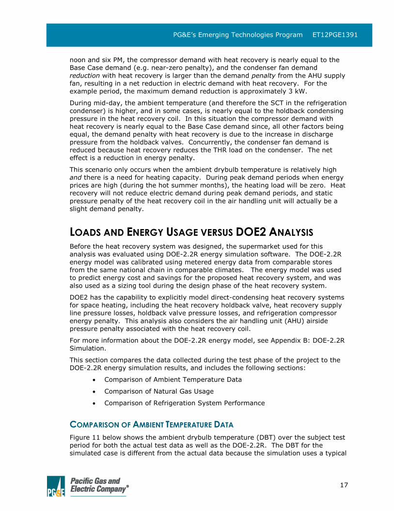
Figure 11 below shows the ambient drybulb temperature (DBT) over the subject test

period for both the actual test data as well as the DOE-2.2R. The DBT for the

simulated case is different from the actual data because the simulation uses a typical

18


meteorological year data file which contains aggregated weather information from

many years of measured data.

FIGURE 11: AMBIENT DRYBULB TEMPERATURE FOR SUBJECT TEST PERIOD FROM ACTUAL DATA AND DOE-2.2R ANALYSIS

Figure 11 shows that the actual DBT and the DOE-2 simulated DBT trend similarly, in

general, with comparable differences in daytime and nighttime temperature swings.

However, the chart shows that the DOE-2 simulated DBT is uniformly lower than the

actual DBT.

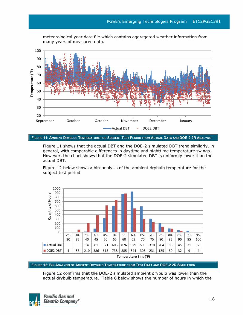
Figure 12 below shows a bin-analysis of the ambient drybulb temperature for the

subject test period.

FIGURE 12: BIN ANALYSIS OF AMBIENT DRYBULB TEMPERATURE FROM TEST DATA AND DOE-2.2R SIMULATION

Figure 12 confirms that the DOE-2 simulated ambient drybulb was lower than the

actual drybulb temperature. Table 6 below shows the number of hours in which the

20

30

40

50

60

70

80

90

100

September October October November December January

Tem

pe

ratu

re (

°F)

Actual DBT DOE2 DBT

25-30

30-35

35-40

40-45

45-50

50-55

55-60

60-65

65-70

70-75

75-80

80-85

85-90

90-95

95-100

Actual DBT 14 81 321 605 876 929 593 310 204 86 45 31 2

DOE2 DBT 4 58 210 386 613 738 885 544 305 231 125 80 32 9 4

0100200300400500600700800900

1000

Qu

anti

ty o

f H

ou

rs

Temperature Bins (°F)

19


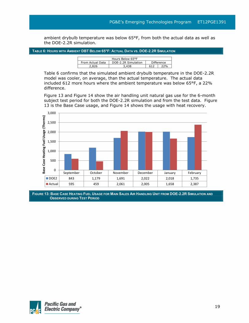
ambient drybulb temperature was below 65°F, from both the actual data as well as

the DOE-2.2R simulation.

TABLE 6: HOURS WITH AMBIENT DBT BELOW 65°F: ACTUAL DATA VS. DOE-2.2R SIMULATION

Hours Below 65°F

From Actual Data DOE-2.2R Simulation Difference

2,826 3,438 612 22%

Table 6 confirms that the simulated ambient drybulb temperature in the DOE-2.2R

model was cooler, on average, than the actual temperature. The actual data

included 612 more hours where the ambient temperature was below 65°F, a 22%

difference.

Figure 13 and Figure 14 show the air handling unit natural gas use for the 6-month

subject test period for both the DOE-2.2R simulation and from the test data. Figure

13 is the Base Case usage, and Figure 14 shows the usage with heat recovery.

FIGURE 13: BASE CASE HEATING FUEL USAGE FOR MAIN SALES AIR HANDLING UNIT FROM DOE-2.2R SIMULATION AND

OBSERVED DURING TEST PERIOD


DOE2 843 1,179 1,691 2,022 2,018 1,735

Actual 595 459 2,061 2,005 1,658 2,387

0

500

1,000

1,500

2,000

2,500

3,000

Bas

e C

ase

He

atin

g Fu

el U

sage

(Th

erm

s)

20


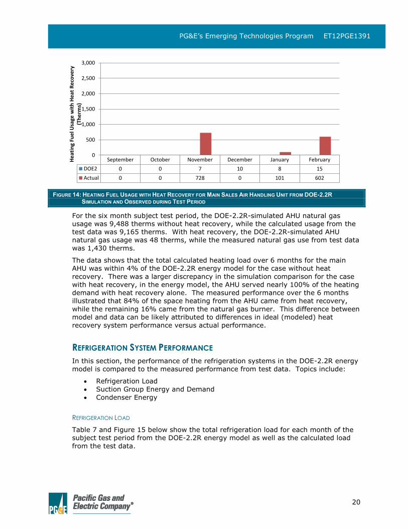
FIGURE 14: HEATING FUEL USAGE WITH HEAT RECOVERY FOR MAIN SALES AIR HANDLING UNIT FROM DOE-2.2R

SIMULATION AND OBSERVED DURING TEST PERIOD

For the six month subject test period, the DOE-2.2R-simulated AHU natural gas

usage was 9,488 therms without heat recovery, while the calculated usage from the

test data was 9,165 therms. With heat recovery, the DOE-2.2R-simulated AHU

natural gas usage was 48 therms, while the measured natural gas use from test data

was 1,430 therms.

The data shows that the total calculated heating load over 6 months for the main

AHU was within 4% of the DOE-2.2R energy model for the case without heat

recovery. There was a larger discrepancy in the simulation comparison for the case

with heat recovery, in the energy model, the AHU served nearly 100% of the heating

demand with heat recovery alone. The measured performance over the 6 months

illustrated that 84% of the space heating from the AHU came from heat recovery,

while the remaining 16% came from the natural gas burner. This difference between

model and data can be likely attributed to differences in ideal (modeled) heat

recovery system performance versus actual performance.

REFRIGERATION SYSTEM PERFORMANCE

In this section, the performance of the refrigeration systems in the DOE-2.2R energy

model is compared to the measured performance from test data. Topics include:

Refrigeration Load

Suction Group Energy and Demand

Condenser Energy

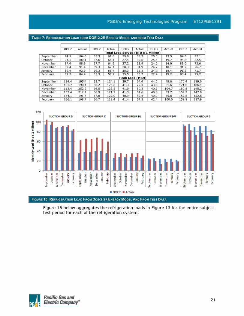
REFRIGERATION LOAD

Table 7 and Figure 15 below show the total refrigeration load for each month of the

subject test period from the DOE-2.2R energy model as well as the calculated load

from the test data.


DOE2 0 0 7 10 8 15

Actual 0 0 728 0 101 602

0

500

1,000

1,500

2,000

2,500

3,000

He

atin

g Fu

el U

sage

wit

h H

eat

Re

cove

ry

(Th

erm

s)

21


TABLE 7: REFRIGERATION LOAD FROM DOE-2.2R ENERGY MODEL AND FROM TEST DATA

DOE2 Actual DOE2 Actual DOE2 Actual DOE2 Actual DOE2 Actual

Total Load Served (BTU x 1 Million)

September 94.5 104.6 35.3 61.6 25.9 35.7 25.0 23.5 94.3 92.1

October 94.1 100.1 37.6 65.1 27.4 35.6 25.4 19.7 94.8 82.5

November 87.4 88.9 37.7 64.6 27.2 33.9 24.0 14.0 89.0 73.6

December 89.4 91.4 39.3 67.1 28.3 34.9 24.7 18.1 91.2 76.7

January 89.4 92.9 39.3 65.4 28.3 35.3 24.7 18.4 91.2 71.7

February 82.2 84.4 35.3 59.2 25.5 30.7 22.4 19.2 83.4 75.2

Peak Load (MBH)

September 184.4 195.4 55.7 124.1 39.7 64.4 44.0 48.6 170.4 189.0

October 181.7 190.1 56.2 126.6 41.3 79.3 43.8 81.6 171.0 186.1

November 153.4 252.2 56.5 123.5 41.0 80.3 40.3 104.7 150.8 145.2

December 157.4 212.1 56.9 121.7 41.3 64.6 40.8 53.7 154.3 147.8

January 164.1 191.4 57.0 122.0 40.9 80.4 40.9 55.8 157.8 152.8

February 166.1 168.7 56.7 118.4 41.4 64.5 42.4 100.0 159.8 187.9

FIGURE 15: REFRIGERATION LOAD FROM DOE-2.2R ENERGY MODEL AND FROM TEST DATA

Figure 16 below aggregates the refrigeration loads in Figure 13 for the entire subject

test period for each of the refrigeration system.

22


FIGURE 16: TOTAL REFRIGERATION LOAD FOR SUBJECT TEST PERIOD FROM DOE-2.2R ENERGY MODEL AND FROM TEST

DATA

For the subject test period, the total refrigeration load served by the refrigeration

systems was 1,736 million BTUs. The DOE-2.2R energy model predicted a

refrigeration load of 1,614 million BTUs, within 8% of the test data.

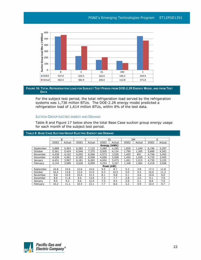
SUCTION GROUP ELECTRIC ENERGY AND DEMAND

Table 8 and Figure 17 below show the total Base Case suction group energy usage

for each month of the subject test period.

TABLE 8: BASE CASE SUCTION GROUP ELECTRIC ENERGY AND DEMAND

B C DL DM E


Energy (kWh)

September 5,888 5,903 6,582 7,122 5,080 4,285 1,850 1,549 6,196 5,297

October 5,361 5,424 6,546 7,375 5,005 4,124 1,790 1,265 5,689 4,542

November 4,438 4,162 6,055 6,596 4,573 3,526 1,455 841 4,748 3,493

December 4,428 4,061 6,183 6,508 4,656 3,508 1,454 1,039 4,735 3,445

January 4,451 3,997 6,181 6,265 4,654 3,473 1,451 1,015 4,730 3,155

February 4,144 3,989 5,628 6,099 4,253 3,227 1,348 1,064 4,418 3,596

Peak (kW)

September 16.8 14.6 12.6 14.6 9.5 8.7 5.3 3.8 17.3 11.8

October 16.4 13.8 12.0 15.0 9.3 10.5 5.0 4.5 16.6 11.3

November 9.8 14.8 10.6 14.3 8.1 9.8 3.1 4.6 10.6 9.0

December 8.6 11.8 9.6 13.8 7.3 7.7 2.8 3.0 9.1 7.9

January 8.9 9.2 9.6 12.4 7.3 9.4 2.8 3.1 8.8 7.5

February 10.2 11.1 10.4 13.1 7.7 8.6 3.2 4.9 10.4 9.7

B C DL DM E

DOE2 537.0 224.5 162.6 146.2 543.9

Actual 562.3 382.9 206.0 112.8 471.8

0

100

200

300

400

500

600

Suct

ion

Gro

up

Lo

ad (

Btu

x 1

Mill

ion

)

23


FIGURE 17: TOTAL BASE CASE SUCTION GROUP ENERGY FOR SUBJECT TEST PERIOD

Table 9 and Figure 18 below show the suction group energy usage with heat

recovery for each month of the subject test period.

TABLE 9: SUCTION GROUP ELECTRIC ENERGY AND DEMAND WITH HEAT RECOVERY

B C DL DM E


Energy (kWh)

September 6,439 6,329 7,068 7,328 5,472 4,295 2,027 1,554 6,768 5,312

October 6,217 5,973 7,318 7,695 5,615 4,125 1,998 1,266 6,595 4,547

November 5,719 5,364 7,223 7,400 5,477 3,562 1,874 853 6,112 3,590

December 5,909 5,603 7,549 7,438 5,703 3,582 1,940 1,065 6,313 3,755

January 5,982 4,693 7,582 6,695 5,730 3,517 1,951 1,028 6,354 3,293

February 5,397 5,482 6,768 6,772 5,134 3,298 1,756 1,095 5,753 3,856

Peak (kW)

September 16.7 14.6 12.6 15.7 9.6 8.7 5.3 3.8 17.3 11.8

October 16.5 13.8 12.1 15.2 9.4 10.5 5.1 4.5 16.7 11.3

November 9.9 15.9 11.1 14.6 8.5 9.8 3.1 4.7 10.7 9.0

December 10.2 13.6 11.2 14.9 8.5 7.7 3.2 3.2 10.6 9.1

January 10.5 9.4 11.2 14.1 8.5 9.4 3.1 3.1 10.8 7.8

February 10.5 11.7 11.1 14.6 8.5 8.6 3.2 5.0 10.9 10.5

B C DL DM E

DOE2 28,710 37,175 28,221 9,348 30,516

Actual 27,536 39,965 22,142 6,773 23,529

0

5,000

10,000

15,000

20,000

25,000

30,000

35,000

40,000

45,000

Ene

rgy

Usa

ge (

kWh

)

24


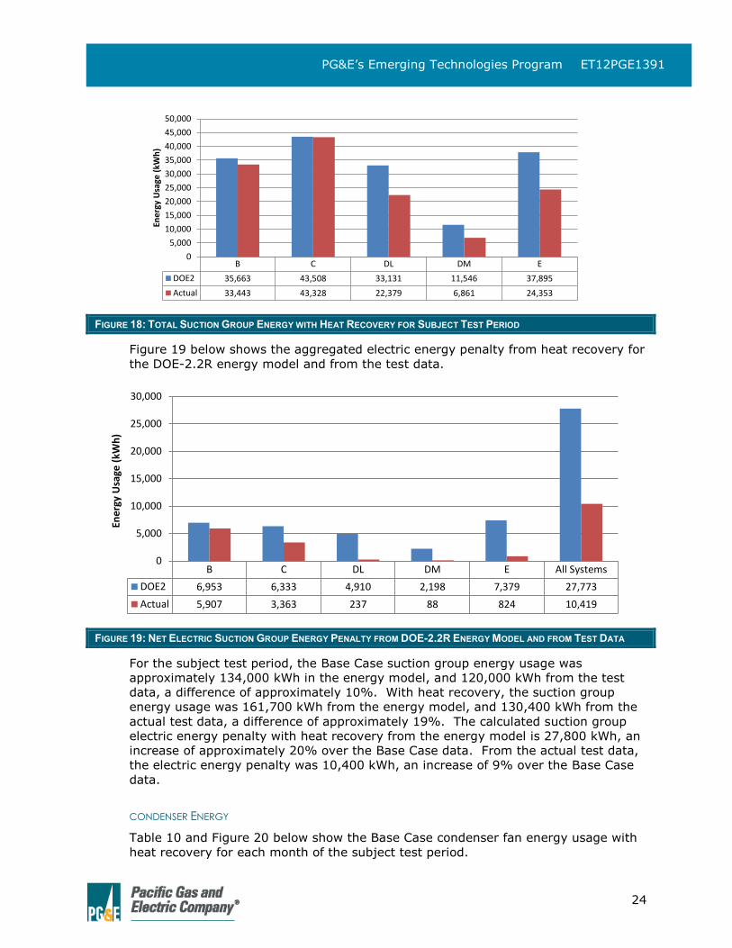
FIGURE 18: TOTAL SUCTION GROUP ENERGY WITH HEAT RECOVERY FOR SUBJECT TEST PERIOD

Figure 19 below shows the aggregated electric energy penalty from heat recovery for

the DOE-2.2R energy model and from the test data.

FIGURE 19: NET ELECTRIC SUCTION GROUP ENERGY PENALTY FROM DOE-2.2R ENERGY MODEL AND FROM TEST DATA

For the subject test period, the Base Case suction group energy usage was

approximately 134,000 kWh in the energy model, and 120,000 kWh from the test

data, a difference of approximately 10%. With heat recovery, the suction group

energy usage was 161,700 kWh from the energy model, and 130,400 kWh from the

actual test data, a difference of approximately 19%. The calculated suction group

electric energy penalty with heat recovery from the energy model is 27,800 kWh, an

increase of approximately 20% over the Base Case data. From the actual test data,

the electric energy penalty was 10,400 kWh, an increase of 9% over the Base Case

data.

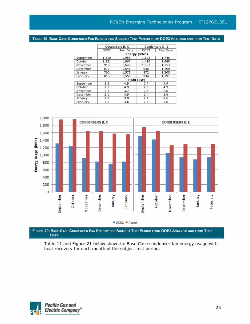
CONDENSER ENERGY

Table 10 and Figure 20 below show the Base Case condenser fan energy usage with

heat recovery for each month of the subject test period.

B C DL DM E

DOE2 35,663 43,508 33,131 11,546 37,895

Actual 33,443 43,328 22,379 6,861 24,353

0

5,000

10,000

15,000

20,000

25,000

30,000

35,000

40,000

45,000

50,000

Ene

rgy

Usa

ge (

kWh

)

B C DL DM E All Systems

DOE2 6,953 6,333 4,910 2,198 7,379 27,773

Actual 5,907 3,363 237 88 824 10,419

0

5,000

10,000

15,000

20,000

25,000

30,000

Ene

rgy

Usa

ge (

kWh

)

25


TABLE 10: BASE CASE CONDENSER FAN ENERGY FOR SUBJECT TEST PERIOD FROM DOE2 ANALYSIS AND FROM TEST DATA

Condensers B, C Condensers D, E

DOE2 Test Data DOE2 Test Data

Energy (kWh)

September 1,310 1,958 1,502 1,746

October 1,231 1,967 1,410 1,648

November 919 1,649 1,052 1,253

December 817 1,641 936 1,290

January 760 1,575 872 1,205

February 818 1,558 934 1,291

Peak (kW)

September 2.5 4.9 2.7 4.9

October 2.5 4.9 2.8 4.9

November 2.1 3.7 2.4 2.8

December 2.1 4.9 2.4 2.6

January 2.2 3.9 2.4 2.6

February 2.2 4.6 2.5 2.8

FIGURE 20: BASE CASE CONDENSER FAN ENERGY FOR SUBJECT TEST PERIOD FROM DOE2 ANALYSIS AND FROM TEST

DATA

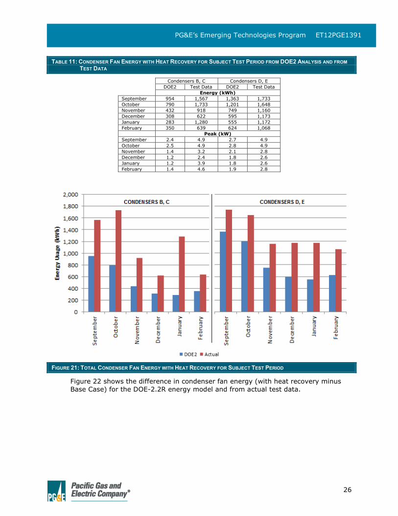
Table 11 and Figure 21 below show the Base Case condenser fan energy usage with

heat recovery for each month of the subject test period.

26


TABLE 11: CONDENSER FAN ENERGY WITH HEAT RECOVERY FOR SUBJECT TEST PERIOD FROM DOE2 ANALYSIS AND FROM

TEST DATA

Condensers B, C Condensers D, E

DOE2 Test Data DOE2 Test Data

Energy (kWh)

September 954 1,567 1,363 1,733

October 790 1,733 1,201 1,648

November 432 918 749 1,160

December 308 622 595 1,173

January 283 1,280 555 1,172

February 350 639 624 1,068

Peak (kW)

September 2.4 4.9 2.7 4.9

October 2.5 4.9 2.8 4.9

November 1.4 3.2 2.1 2.8

December 1.2 2.4 1.8 2.6

January 1.2 3.9 1.8 2.6

February 1.4 4.6 1.9 2.8

FIGURE 21: TOTAL CONDENSER FAN ENERGY WITH HEAT RECOVERY FOR SUBJECT TEST PERIOD

Figure 22 shows the difference in condenser fan energy (with heat recovery minus

Base Case) for the DOE-2.2R energy model and from actual test data.

27


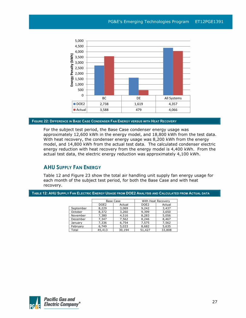
FIGURE 22: DIFFERENCE IN BASE CASE CONDENSER FAN ENERGY VERSUS WITH HEAT RECOVERY

For the subject test period, the Base Case condenser energy usage was

approximately 12,600 kWh in the energy model, and 18,800 kWh from the test data.

With heat recovery, the condenser energy usage was 8,200 kWh from the energy

model, and 14,800 kWh from the actual test data. The calculated condenser electric

energy reduction with heat recovery from the energy model is 4,400 kWh. From the

actual test data, the electric energy reduction was approximately 4,100 kWh.

AHU SUPPLY FAN ENERGY

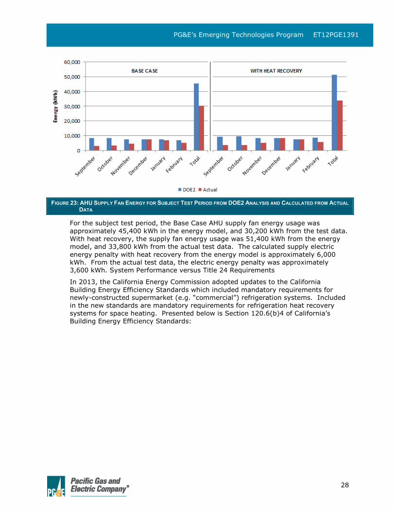
Table 12 and Figure 23 show the total air handling unit supply fan energy usage for

each month of the subject test period, for both the Base Case and with heat

recovery.

TABLE 12: AHU SUPPLY FAN ELECTRIC ENERGY USAGE FROM DOE2 ANALYSIS AND CALCULATED FROM ACTUAL DATA

Base Case With Heat Recovery

DOE2 Actual DOE2 Actual

September 8,229 3,069 9,242 3,437

October 8,372 3,260 9,399 3,650

November 7,380 4,516 8,283 5,056

December 7,347 7,562 8,246 8,467

January 7,336 6,754 7,575 7,562

February 6,749 5,033 8,682 5,635

Total 45,413 30,194 51,427 33,808

BC DE All Systems

DOE2 2,738 1,619 4,357

Actual 3,588 479 4,066

0

500

1,000

1,500

2,000

2,500

3,000

3,500

4,000

4,500

5,000

Ene

rgy

Pe

nal

ty (

kWh

)

28


FIGURE 23: AHU SUPPLY FAN ENERGY FOR SUBJECT TEST PERIOD FROM DOE2 ANALYSIS AND CALCULATED FROM ACTUAL

DATA

For the subject test period, the Base Case AHU supply fan energy usage was

approximately 45,400 kWh in the energy model, and 30,200 kWh from the test data.

With heat recovery, the supply fan energy usage was 51,400 kWh from the energy

model, and 33,800 kWh from the actual test data. The calculated supply electric

energy penalty with heat recovery from the energy model is approximately 6,000

kWh. From the actual test data, the electric energy penalty was approximately

3,600 kWh. System Performance versus Title 24 Requirements

In 2013, the California Energy Commission adopted updates to the California

Building Energy Efficiency Standards which included mandatory requirements for

newly-constructed supermarket (e.g. “commercial”) refrigeration systems. Included

in the new standards are mandatory requirements for refrigeration heat recovery

systems for space heating. Presented below is Section 120.6(b)4 of California’s

Building Energy Efficiency Standards:

29


4. Refrigeration Heat Recovery.

A. HVAC systems shall utilize heat recovery from refrigeration system(s) for space heating, using no less than 25 percent of the sum of the design Total Heat of Rejection of all refrigeration systems that have individual Total Heat of Rejection values of 150,000 Btu/h or greater at design conditions.

EXCEPTION 1 to Section 120.6(b)4A: Stores located in Climate Zone 15.

EXCEPTION 2 to Section 120.6(b)4A: HVAC systems or refrigeration systems that are reused for an addition or alteration.

B. The increase in hydrofluorocarbon refrigerant charge associated with refrigeration heat recovery equipment and piping shall be no greater than 0.35 lbs per 1,000 Btu/h of heat recovery heating capacity.

The heat recovery requirement of Title 24 (Section 120.6(b)4) applies to newly-

constructed supermarkets, and newly-constructed additions to existing supermarkets

where additional refrigeration capacity and space heating capacity are both included

in the expansion design. The requirement does not apply to retrofits.

Also included in the new standards are requirements for condenser efficiency and

control. Relevant to this study is the requirement that refrigeration head pressure

shall be allowed to float to 70°F SCT or less, with mandatory ambient-following (e.g.

variable setpoint or drybulb reset logic) controls and variable-speed condenser fan

control.

The supermarket used for this study was permitted for construction before January

1, 2014, and is therefore not required to comply with the Title-24 standards.

However, the heat recovery system was scrutinized in the context of the Title 24

requirements in the following sections, which include:

Heat Recovered versus Whole-Building THR

Refrigerant Charge Analysis

HEAT RECOVERED VERSUS WHOLE BUILDING THR

Per Title 24 requirements, heat recovery capacity at design conditions shall be at

least 25% of the total heat rejection (THR) of all the refrigeration systems in the

building whose THR is higher than 150 MBH. The design documentation for the

subject store states that the THR at design conditions is 1,980 MBH, and the design

heat recovery coil capacity is 781 MBH—39% of the whole-store design THR.

Therefore, the subject recovery system would comply with the minimum heat

recovery capacity requirements in Title 24.

REFRIGERANT CHARGE ANALYSIS

Subsection B of the Title 24 heat recovery standards prohibits heat recovery designs

which increase hydrofluorocarbon (HFC) refrigerant charge by more than 0.35 lbs for

30


every MBH of heat recovery heating capacity added, at design conditions, versus a

comparably-sized refrigeration system without heat recovery. The requirement is

motivated by the recognition that more refrigerant charge increases refrigerant

emissions to the atmosphere, with HFC refrigerants exhibiting global warming

potentials that are several thousand times higher than carbon dioxide (the global

warming potential of R-507A, the refrigerant in the subject test system, is almost

4,000 times higher than CO2).

Refrigerant charge goes up due to the addition of the recovery coil itself and the

additional piping between the compressors and the recovery coil. In addition, the

refrigerant leaving the recovery coil and entering the refrigerant condenser is mostly

condensed, which increases the charge in the outdoor condenser compared with

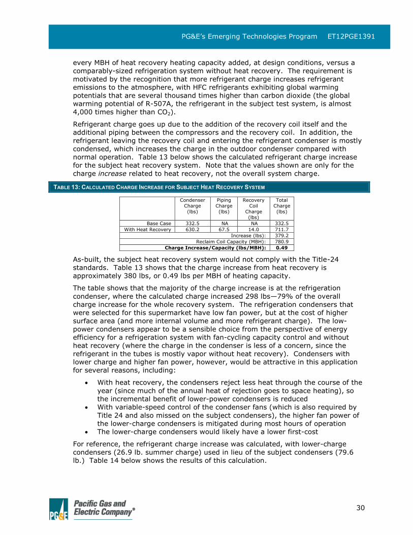
normal operation. Table 13 below shows the calculated refrigerant charge increase

for the subject heat recovery system. Note that the values shown are only for the

charge increase related to heat recovery, not the overall system charge.

TABLE 13: CALCULATED CHARGE INCREASE FOR SUBJECT HEAT RECOVERY SYSTEM

Condenser

Charge

(lbs)

Piping

Charge

(lbs)

Recovery

Coil

Charge

(lbs)

Total

Charge

(lbs)

Base Case 332.5 NA NA 332.5

With Heat Recovery 630.2 67.5 14.0 711.7

Increase (lbs): 379.2

Reclaim Coil Capacity (MBH): 780.9

Charge Increase/Capacity (lbs/MBH): 0.49

As-built, the subject heat recovery system would not comply with the Title-24

standards. Table 13 shows that the charge increase from heat recovery is

approximately 380 lbs, or 0.49 lbs per MBH of heating capacity.

The table shows that the majority of the charge increase is at the refrigeration

condenser, where the calculated charge increased 298 lbs—79% of the overall

charge increase for the whole recovery system. The refrigeration condensers that

were selected for this supermarket have low fan power, but at the cost of higher

surface area (and more internal volume and more refrigerant charge). The low-

power condensers appear to be a sensible choice from the perspective of energy

efficiency for a refrigeration system with fan-cycling capacity control and without

heat recovery (where the charge in the condenser is less of a concern, since the

refrigerant in the tubes is mostly vapor without heat recovery). Condensers with

lower charge and higher fan power, however, would be attractive in this application

for several reasons, including:

With heat recovery, the condensers reject less heat through the course of the

year (since much of the annual heat of rejection goes to space heating), so

the incremental benefit of lower-power condensers is reduced

With variable-speed control of the condenser fans (which is also required by

Title 24 and also missed on the subject condensers), the higher fan power of

the lower-charge condensers is mitigated during most hours of operation

The lower-charge condensers would likely have a lower first-cost

For reference, the refrigerant charge increase was calculated, with lower-charge

condensers (26.9 lb. summer charge) used in lieu of the subject condensers (79.6

lb.) Table 14 below shows the results of this calculation.

31


TABLE 14: CALCULATED CHARGE INCREASE FOR SUBJECT HEAT RECOVERY SYSTEM WITH LOW-CHARGE CONDENSERS

Condenser Charge

(lbs)

Piping Charge

(lbs)

Recovery Coil

Charge

(lbs)

Total Charge

(lbs)

Base Case 112.4 NA NA 112.4

With Heat Recovery 213.0 67.5 14.0 294.5

Increase (lbs): 182.1

Reclaim Coil Capacity (MBH): 780.9

Charge Increase/Capacity (lbs/MBH): 0.23

With lower-charge condensers, the subject test system could easily comply with the

Title 24 requirements, with the calculated charge increasing only 0.23 lbs per MBH of

heat rejection capacity—33% lower than the Title 24 requirement and 52% lower

than the as-built design.

Moreover, the series-connected, direct-condensing heat recovery design analyzed

here results in the largest increase in refrigerant charge relative to other recovery

designs. Alternative designs include heat recovery heat exchangers that are piped in

parallel with the refrigeration condensers (e.g. parallel-connected direct-condensing),

and indirect heat recovery systems where heat is exchanged first with a water or

water/glycol loop in a close-coupled refrigerant/water heat exchanger, and then

pumped to water/air heat exchangers in one or more air handling units. Parallel-

connected heat recovery systems require no additional refrigerant charge since the

refrigeration condenser is not used when heat recovery is on. Indirect heat recovery

designs also require little additional refrigerant, since the refrigerant-to-fluid heat

exchanger can be mounted close to the compressors, reducing refrigerant charge in

the piping between the compressor racks and the heat recovery heat exchanger.

For reference, the total charge for each system is shown in Table 15 below. The

information was provided by the refrigeration contractor.

TABLE 15: R-507A REFRIGERANT CHARGE PER SYSTEM IN POUNDS

System

Charge

(lbs)

A 350

B 575

C 600

D 575

E 550

F 450

ECONOMICS ANALYSIS In this section, a cost estimate and economic analysis of the project is performed.

Table 16 below shows an estimation of the installation costs for the heat recovery

system.

32


TABLE 16: HEAT RECOVERY PROJECT COST ESTIMATE

Item Quantity Cost per Unit ($)

Cost ($)

Materials

4-circuit direct-condensing reclaim coil (materials and installation) 1 $4,300 $4,300

Three-Way Refrigerant Control Valves 4 $250 $1,000

Electronic Holdback Valves 4 $350 $1,400

Check Valves 4 $60 $240

Pump-Out Solenoid Valves 4 $75 $300

Additional Piping and Insulation $3,890 $3,890

Additional Refrigerant 182 lbs. $3.79/lb $690

Labor

Engineering 40 hours $95/hr $3,800

Piping Installation 16 hours $60/hr $960

Controls programming, tuning 10 hours $115/hr $1,150

Total Estimated Cost: $17,730

Table 17 below shows the calculated simple payback, net present value (NPV) and

internal rate of return (IRR) for this project. The utility cost savings represent the

expectation based on DOE2.2R modeling analysis, which represents the annual

expectations for savings and operating cost. The NPV and IRR results are based on

an assumed escalation rate of 4% and a discount rate of 8% over 15 years.

TABLE 17: SIMPLE PAYBACK, NET PRESENT VALUE, AND INTERNAL RATE OF RETURN ANALYSIS WITHOUT INCENTIVES

Annual Utility Cost Savings vs. Base Case $9,395

Heat Recovery Additional Capital Cost $17,730

Simple Payback 1.9

Net Present Value (NPV) $83,799

Internal Rate of Return (IRR) 57%

Table 17 shows that the simple payback is less than two years without utility

incentives. Table 18 below shows the calculated simple payback, NPV, and IRR with

utility incentives. The incentive amount was assumed to be $1.00 per therm of

natural gas savings, with a cost limit of 50% of the measure capital cost (which is a

factor for this analysis).

TABLE 18: SIMPLE PAYBACK, NET PRESENT VALUE, AND INTERNAL RATE OF RETURN ANALYSIS WITH INCENTIVES

Annual Utility Cost Savings vs. Base Case $9,395

Heat Recovery Additional Capital Cost $17,730

Utility Incentive $8,865

Additional Capital Cost with Utility Incentives $8,865

Simple Payback 0.9

Net Present Value (NPV) $92,664

Internal Rate of Return (IRR) 110%

With utility incentives, the simple payback could be less than one year.

Furthermore, the economics of heat recovery in other locations would likely be even

more attractive for several reasons, including:

The heating load in the host site’s town is relatively low

o The number of annual heating design hours at 65°F is only 1,196

o The ambient drybulb temperature is normally mild (the average annual

drybulb temperature is 60.3°F, and the 0.4% design drybulb is

88.4°F)

o The humidity (the biggest driver of heating load) is low (0.4% design

RH: 68% at 74.4°F mean coincident drybulb)

Natural gas prices in the host site’s town are relatively low

Electric energy prices in host site’s town are relatively high

33


CONCLUSIONS

In six months of testing, there was a measured heat recovery system offset of 7,740 therms

of natural gas. During that time, the refrigeration system energy usage went up by 10,300

kWh. The Net energy savings was 738.3 Million BTUs. The net energy cost savings was

$6,400. The scope of this evaluation was limited to heat recovery for just the main sales

area air handling unit, although the supermarket HVAC demand is met with several other

additional HVAC units, all of which are equipped with natural gas furnaces and outside air

dampers. Further optimization of the HVAC design approach could yield even more savings

from heat recovery, by utilizing heat recovery capacity to serve the heating load that is

currently served by secondary rooftop units. In addition to this, the same system operating

in different (colder) climates or with different energy rate structures will both perform

differently and have different savings. The system considered in this study was operated in

a relatively mild climate with relative minor heating needs. The same arrangement installed

in a colder climate may demonstrate much larger savings.

Heat recovery for space heating should be adopted as an energy efficiency measure, and

significant statewide energy savings are possible with widespread adoption. While

California’s energy efficiency standards (Title 24) require heat recovery for newly

constructed commercial refrigeration (e.g. supermarket) applications, financial incentives

are recommended for supermarket retrofit applications, and new-construction applications

that are exempt from the Title 24 requirements but still have space heating loads and

refrigeration capacity. However, substantial market support and training by the California

utility companies (beyond just incentives) is needed to achieve the intended savings levels

and market penetration, while balancing electric energy penalty and refrigerant charge

increase. Specifically, the industry seems to have lost much of the technical understanding

related to holdback valve utilization and control.

The focus of this project was a direct-condensing heat recovery system, where heat is

exchanged from refrigerant directly to air. Other heat recovery configurations are viable,

with comparable (or even higher) savings expectations, which would be more suitable for

retrofit applications. One configuration in particular is the indirect design, where recovered

heat is transferred from the refrigerant to an intermediate fluid (normally water or water-

glycol) which is circulated through a fluid-to-air heat exchanger located in the air handling

unit airstream.

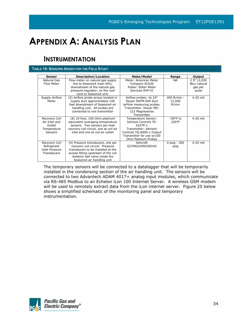
34


APPENDIX A: ANALYSIS PLAN

INSTRUMENTATION TABLE 19: SENSORS ADDED FOR THE FIELD STUDY

Sensor Description/Location Make/Model Range Output

Natural Gas

Flow Meter

Flow meter on natural gas supply

line to Seasons4 main AHU,

downstream of the natural gas pressure regulator, on the roof

next to Seasons4 unit.

Meter: American Meter

Company AC630

Pulser: Elster Meter Services RVP-VI

NA 2 ft3 (2,030

Btu) natural

gas per pulse

Supply Airflow

Meter

(5) Airflow probe arrays located in

supply duct approximately 100

feet downstream of Seasons4 air

handling unit. All probes are

connected to one transmitter

Airflow probes: 4x 24"

Dwyer DAFM-009 duct

airflow measuring probes.

Transmitter: Dwyer MS-

121 Magnesense

Transmitter

400 ft/min -

12,000

ft/min

4-20 mA

Recovery Coil

Air Inlet and

Outlet

Temperature

Sensors

(8) 10-foot, 100-Ohm platinum

equivalent averaging temperature

sensors. Two sensors per heat

recovery coil circuit, one at coil air

inlet and one at coil air outlet

Temperature Sensor:

Johnson Controls TE-

6337P-1

Transmitter: Johnson

Controls TQ-6000-1 Output Transmitter for use w/100

Ohm Platinum Probes

-50°F to

220°F

4-20 mA

Recovery Coil

Refrigerant

Inlet Pressure

Transducers

(4) Pressure transducers, one per

recovery coil circuit. Pressure

transducers to be installed at the

access fitting upstream of the coil

isolation ball valve inside the

Seasons4 air handling unit

Ashcroft

G27M0242M2300#G

0 psig - 300

psig

4-20 mA

The temporary sensors will be connected to a datalogger that will be temporarily

installed in the condensing section of the air handling unit. The sensors will be

connected to two Advantech ADAM 4017+ analog input modules, which communicate

via RS-485 Modbus to an Echelon iLon 100 Internet Server. A wireless GSM modem

will be used to remotely extract data from the iLon internet server. Figure 25 below

shows a simplified schematic of the monitoring panel and temporary

instrumentation.

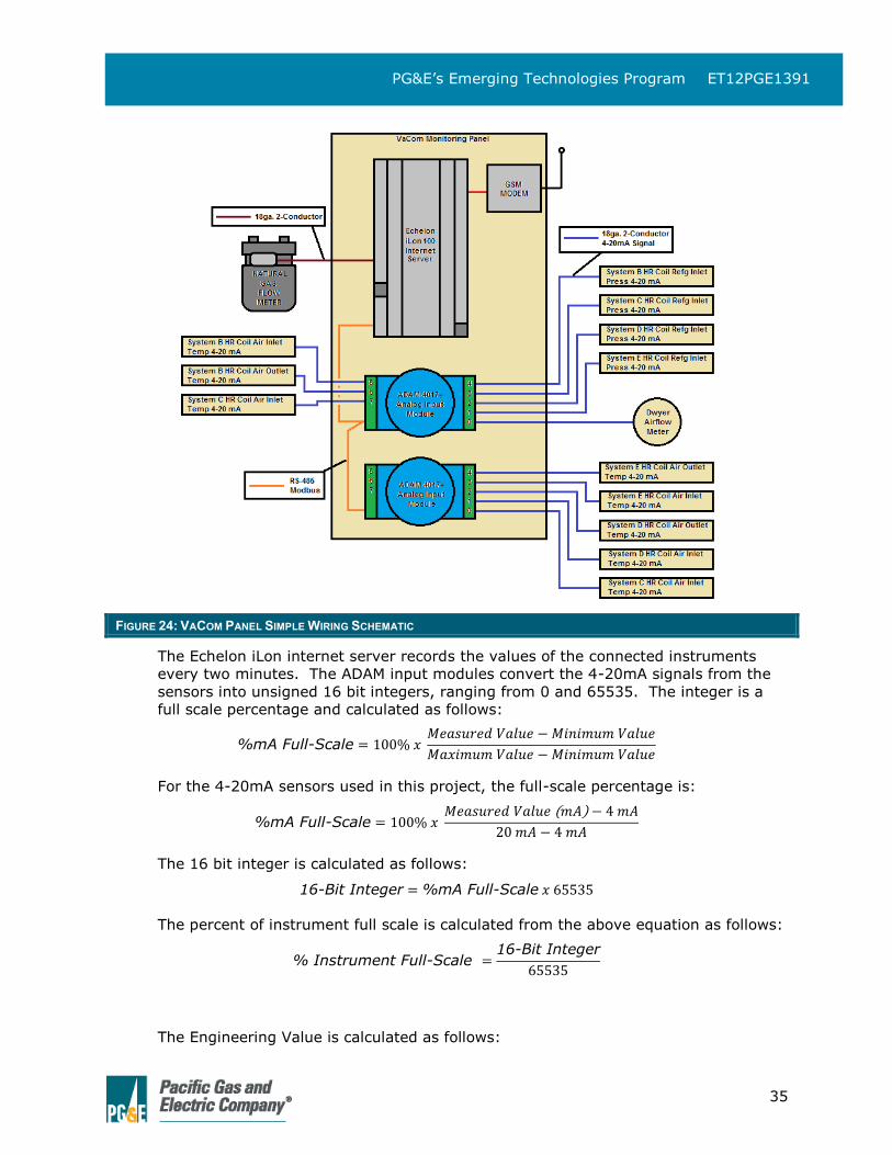
35


FIGURE 24: VACOM PANEL SIMPLE WIRING SCHEMATIC

The Echelon iLon internet server records the values of the connected instruments

every two minutes. The ADAM input modules convert the 4-20mA signals from the

sensors into unsigned 16 bit integers, ranging from 0 and 65535. The integer is a

full scale percentage and calculated as follows:

%mA Full-Scale = 100% 𝑥 𝑀𝑒𝑎𝑠𝑢𝑟𝑒𝑑 𝑉𝑎𝑙𝑢𝑒 − 𝑀𝑖𝑛𝑖𝑚𝑢𝑚 𝑉𝑎𝑙𝑢𝑒

𝑀𝑎𝑥𝑖𝑚𝑢𝑚 𝑉𝑎𝑙𝑢𝑒 − 𝑀𝑖𝑛𝑖𝑚𝑢𝑚 𝑉𝑎𝑙𝑢𝑒

For the 4-20mA sensors used in this project, the full-scale percentage is:

%mA Full-Scale = 100% 𝑥 𝑀𝑒𝑎𝑠𝑢𝑟𝑒𝑑 𝑉𝑎𝑙𝑢𝑒 (𝑚𝐴) − 4 𝑚𝐴

20 𝑚𝐴 − 4 𝑚𝐴

The 16 bit integer is calculated as follows:

16-Bit Integer = %mA Full-Scale 𝑥 65535

The percent of instrument full scale is calculated from the above equation as follows:

% Instrument Full-Scale =16-Bit Integer

65535

The Engineering Value is calculated as follows:

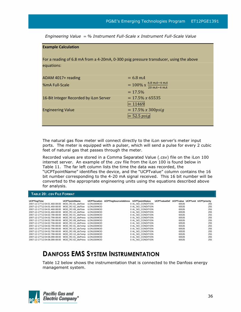
36


Engineering Value = % Instrument Full-Scale x Instrument Full-Scale Value

Example Calculation

For a reading of 6.8 mA from a 4-20mA, 0-300 psig pressure transducer, using the above

equations:

ADAM 4017+ reading = 6.8 𝑚𝐴

%mA Full-Scale = 100% x 6.8 𝑚𝐴−4 𝑚𝐴

20 𝑚𝐴−4 𝑚𝐴

= 17.5%

16-Bit Integer Recorded by iLon Server = 17.5% 𝑥 65535

= 11469

Engineering Value = 17.5% 𝑥 300𝑝𝑠𝑖𝑔

= 52.5 𝑝𝑠𝑖𝑔

The natural gas flow meter will connect directly to the iLon server’s meter input

ports. The meter is equipped with a pulser, which will send a pulse for every 2 cubic

feet of natural gas that passes through the meter.

Recorded values are stored in a Comma Separated Value (.csv) file on the iLon 100

internet server. An example of the .csv file from the iLon 100 is found below in

Table 11. The far left column lists the time the data was recorded, the

“UCPTpointName” identifies the device, and the “UCPTvalue” column contains the 16

bit number corresponding to the 4-20 mA signal received. This 16 bit number will be

converted to the appropriate engineering units using the equations described above

for analysis.

TABLE 20: .CSV FILE FORMAT

DANFOSS EMS SYSTEM INSTRUMENTATION Table 12 below shows the instrumentation that is connected to the Danfoss energy

management system.

UCPTlogTime UCPTpointName UCPTlocation UCPTlogSourceAddress UCPTpointStatus UCPTvalueDef UCPTvalue UCPTunit UCPTpriority

2007-12-17T12:04:01.460-08:00 MOD_RC-01_disFlow iLON100/MOD 0 AL_NO_CONDITION 65535 255




2007-12-17T12:04:02.790-08:00 MOD_RC-01_disPress iLON100/MOD 0 AL_NO_CONDITION 65535 255




2007-12-17T12:04:02.790-08:00 MOD_RC-01_disTemp iLON100/MOD 0 AL_NO_CONDITION 65535 255






37


TABLE 21: INSTRUMENTATION CONNECTED TO DANFOSS EMS SYSTEM

Pressure Temperature Status

Sensors at Refrigeration Compressor Racks

Suction Pressure (1 per

Suction Group, 5 Total)

Suction Temperature Compressor Run Proofs

Discharge Pressure (1 per

Protocol Unit, 4 Total)

Compressor Alarms

Sensors at Condenser

Dropleg Pressure (1 per

Condenser)

Ambient Temperature (1

per Condenser)

Fan Run Proof

Fan Speed

Sensors in Air Handling Unit

Heat Recovery Coil Holdback

Pressure (1 per Circuit, 4

Total)

Sales Area Space

Temperature

Air Flow Switch

Sales Area Space Humidity

Supply Air Temperature

Return Air Temperature

(sensor to be relocated to

account for outside air)

Heat Recovery Coil Inlet

Temperature (1 per Circuit,

4 Total)

Heat Recovery Coil Outlet Temperature (1 per Circuit,

4 Total)

Heat Recovery Coil

Holdback Valve Outlet

Temperature (1 per Circuit,

4 Total)

The refrigeration system controllers are Danfoss AK-SC 255 units. These units have

enough memory to store history data at 1-minute intervals for over one year.

ANALYSIS PLAN

PRE-INSTALLATION INSTRUMENTATION COMMISSIONING

Each instrument will be tested at a known set of conditions to verify they are

functioning properly before they are installed in the field. The data acquisition

system will also be tested for proper operation. An EXTECH CMM-15 signal

generator will be used to generate outputs between 4 mA and 20 mA to verify that

the signal is read accurately by the ADAM-4017+ analog input module and recorded

correctly in the data file written by the iLon 100 e3 internet server. The signals will

also be verified with a digital multimeter. A test log .csv file will be generated with

the recorded values and their corresponding time stamp. This log will be correlated

to the physical test logs to validate the monitoring system from source to data log.

INSTRUMENTATION FIELD COMMISSIONING

After the refrigeration and HVAC systems are installed and the system controls have

been installed, and commissioned, the temporary field instruments will be

commissioned to ensure accuracy and proper operation. During the instrumentation

field commissioning period, several parameters will be measured and recorded,

which will be necessary to calculate net Therm savings and consequent energy

penalty:

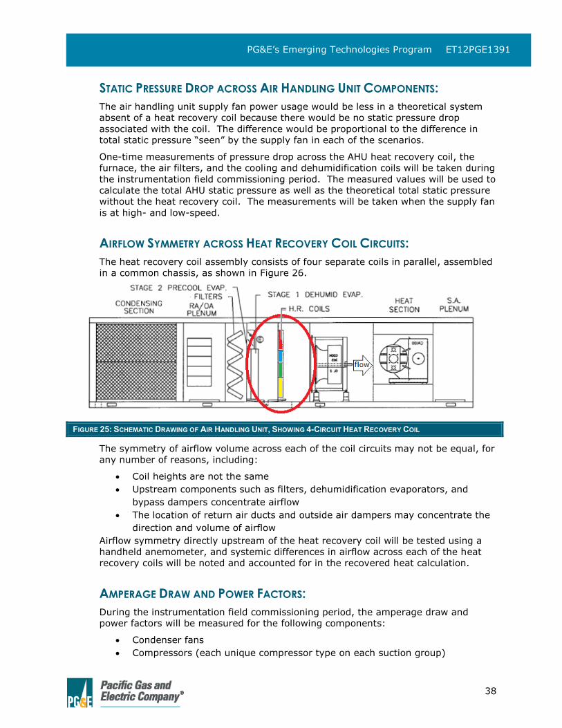
38


STATIC PRESSURE DROP ACROSS AIR HANDLING UNIT COMPONENTS:

The air handling unit supply fan power usage would be less in a theoretical system

absent of a heat recovery coil because there would be no static pressure drop

associated with the coil. The difference would be proportional to the difference in

total static pressure “seen” by the supply fan in each of the scenarios.

One-time measurements of pressure drop across the AHU heat recovery coil, the

furnace, the air filters, and the cooling and dehumidification coils will be taken during

the instrumentation field commissioning period. The measured values will be used to

calculate the total AHU static pressure as well as the theoretical total static pressure

without the heat recovery coil. The measurements will be taken when the supply fan

is at high- and low-speed.

AIRFLOW SYMMETRY ACROSS HEAT RECOVERY COIL CIRCUITS:

The heat recovery coil assembly consists of four separate coils in parallel, assembled

in a common chassis, as shown in Figure 26.

FIGURE 25: SCHEMATIC DRAWING OF AIR HANDLING UNIT, SHOWING 4-CIRCUIT HEAT RECOVERY COIL

The symmetry of airflow volume across each of the coil circuits may not be equal, for

any number of reasons, including:

Coil heights are not the same

Upstream components such as filters, dehumidification evaporators, and

bypass dampers concentrate airflow

The location of return air ducts and outside air dampers may concentrate the

direction and volume of airflow

Airflow symmetry directly upstream of the heat recovery coil will be tested using a

handheld anemometer, and systemic differences in airflow across each of the heat

recovery coils will be noted and accounted for in the recovered heat calculation.

AMPERAGE DRAW AND POWER FACTORS:

During the instrumentation field commissioning period, the amperage draw and

power factors will be measured for the following components:

Condenser fans

Compressors (each unique compressor type on each suction group)

39


Seasons4 air handling unit supply fan (at high- and low-speed)

DATA COLLECTION

The data measured by the added instrumentation will be transmitted via wireless

modem to VaCom’s EnergyDashboard (EDB) server for processing and automated

analysis. In addition, operations data from the Danfoss control system will be

manually downloaded weekly and sent to EDB for processing as well (Danfoss is

developing a PC-based software tool called AK-EM 800 that can automatically

download history files from Danfoss EMS systems. This tool may be used in lieu of

manual download when it is available). The processed data and efficiency

comparisons of the test and reference systems will be viewable using web access to

EnergyDashboard, and will be designed to allow user selection of time intervals and

levels of comparison.

MEASURING HEAT RECOVERY PERFORMANCE

The primary measurement metrics for this study are Therms of natural gas heating

energy saved by heat recovery, and the additional energy consumed by the

refrigeration suction groups and air handling unit supply fan as a result of heat

recovery. The natural gas savings will be found by calculating the total heat

recovered from the refrigeration system, and then calculating the equivalent amount

of natural gas required by the furnace to add the same quantity of heat in the Base

Case. The additional energy will be equal to the sum total of the required energy for

the refrigeration compressors, refrigeration condensers, and air handling unit supply

fan, minus the required energy for the same components in the theoretical Base

Case.

ESTABLISHING BASE CASE PERFORMANCE

For this analysis, the basis of comparison for the heat recovery system is a

theoretical system consisting of the same refrigeration and HVAC components, and

the same ambient conditions, refrigeration loads, and heating loads as the system

with heat recovery, but absent all of the components related to heat recovery. In

order to calculate the performance of the Base Case system, a Base Case

performance establishment period will be held where the heat recovery system is

disabled for approximately 2 weeks. Data collected during this period will be used to

calculate several performance metrics for the Base Case system, which are described

below:

REFRIGERATION SYSTEM CONDENSER CAPACITY:

Condenser capacity is a function of the condenser fan speed as well as the

temperature difference (TD) between the actual refrigerant saturated condensing

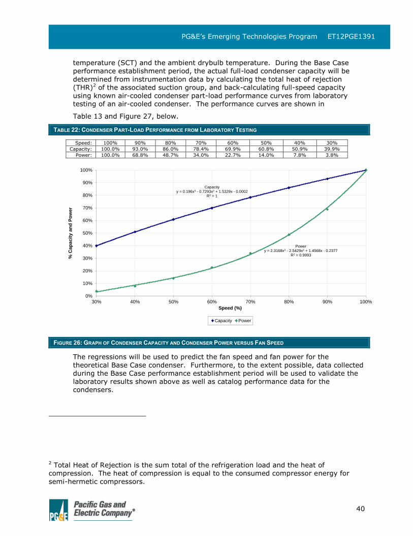
40


temperature (SCT) and the ambient drybulb temperature. During the Base Case

performance establishment period, the actual full-load condenser capacity will be

determined from instrumentation data by calculating the total heat of rejection

(THR)2 of the associated suction group, and back-calculating full-speed capacity

using known air-cooled condenser part-load performance curves from laboratory

testing of an air-cooled condenser. The performance curves are shown in

Table 13 and Figure 27, below.

TABLE 22: CONDENSER PART-LOAD PERFORMANCE FROM LABORATORY TESTING

Speed: 100% 90% 80% 70% 60% 50% 40% 30%

Capacity: 100.0% 93.0% 86.0% 78.4% 69.9% 60.8% 50.9% 39.9%

Power: 100.0% 68.8% 48.7% 34.0% 22.7% 14.0% 7.8% 3.8%

FIGURE 26: GRAPH OF CONDENSER CAPACITY AND CONDENSER POWER VERSUS FAN SPEED

The regressions will be used to predict the fan speed and fan power for the

theoretical Base Case condenser. Furthermore, to the extent possible, data collected

during the Base Case performance establishment period will be used to validate the

laboratory results shown above as well as catalog performance data for the

condensers.

2 Total Heat of Rejection is the sum total of the refrigeration load and the heat of

compression. The heat of compression is equal to the consumed compressor energy for

semi-hermetic compressors.

Capacityy = 0.196x3 - 0.7293x2 + 1.5329x - 0.0002

R2 = 1

Powery = 2.3168x3 - 2.5429x2 + 1.4568x - 0.2377

R2 = 0.9993

0%

10%

20%

30%

40%

50%

60%

70%

80%

90%

100%

30% 40% 50% 60% 70% 80% 90% 100%

% C

ap

ac

ity a

nd

Po

we

r

Speed (%)

Capacity Power

41


BASE CASE FURNACE EFFICIENCY:

Over the course of the Base Case performance establishment period, furnace

efficiency will be calculated by dividing the energy input into the airstream by the

total potential heat from the natural gas stream. Energy input will be calculated

from the supply air flowrate, the mixed return/outside air temperature, and the

supply air temperature. Potential heat from the natural gas stream will be a known

quantity from the natural gas flow meter and the thermodynamic properties of

natural gas.

In the Seasons4 main air handling unit, the natural gas furnace is downstream of the

heat recovery coil. In the Base Case, the furnace efficiency is expected to be higher

than when heat recovery is on because the system exergy will be higher; the

temperature of the air entering the furnace will be lower in the Base Case, meaning

the temperature difference between the air and the furnace will be larger. The larger

TD will result in more energy entering the supply airstream per unit of natural gas

burned, and thus higher efficiency.

BASE CASE REFRIGERATION SYSTEM OPTIMUM CONTROL TD

The refrigeration control temperature difference (control TD) may be optimized for

each of the four subject refrigeration systems during the Base Case performance

establishment period. The control TD is the temperature difference between the

target refrigeration saturated condensing temperature (SCT) and the ambient

drybulb temperature, and in general is optimized so that the combined total of

compressor and condenser power is as low as possible. In the Base Case, the

refrigeration condenser will reject all of the system total heat of rejection (THR)

whereas the majority of the THR will be absent in the Heat Recovery scenario, as the

heat will be used for space heating. Therefore, the optimum control TD might be

different for the Base Case than when heat recovery is on.

The optimum Base Case control TD may be a moving target. There may be no

opportunity to collect data when the target SCT is in the control range3 during the

first few months of operation, since the ambient drybulb temperature will likely be

too low. It may be necessary to collect additional Base Case data during warm-

weather conditions. Having a theoretical Base Case control TD that is different than

the heat recovery scenario would only be justified if there are enough hours where

the refrigeration system is in the control range and heat recovery is on at the same

time to influence the economics. It is possible that the “optimum” control TD will be

more influenced by peak hot-weather conditions when heat recovery is likely to be

off, in which case the Base Case control TD and the heat recovery control TD will be

the same.

3 Control Range is when the target SCT for control is between the programmed maximum

and minimum values, and is therefore calculated from the Control TD and ambient drybulb

temperature.

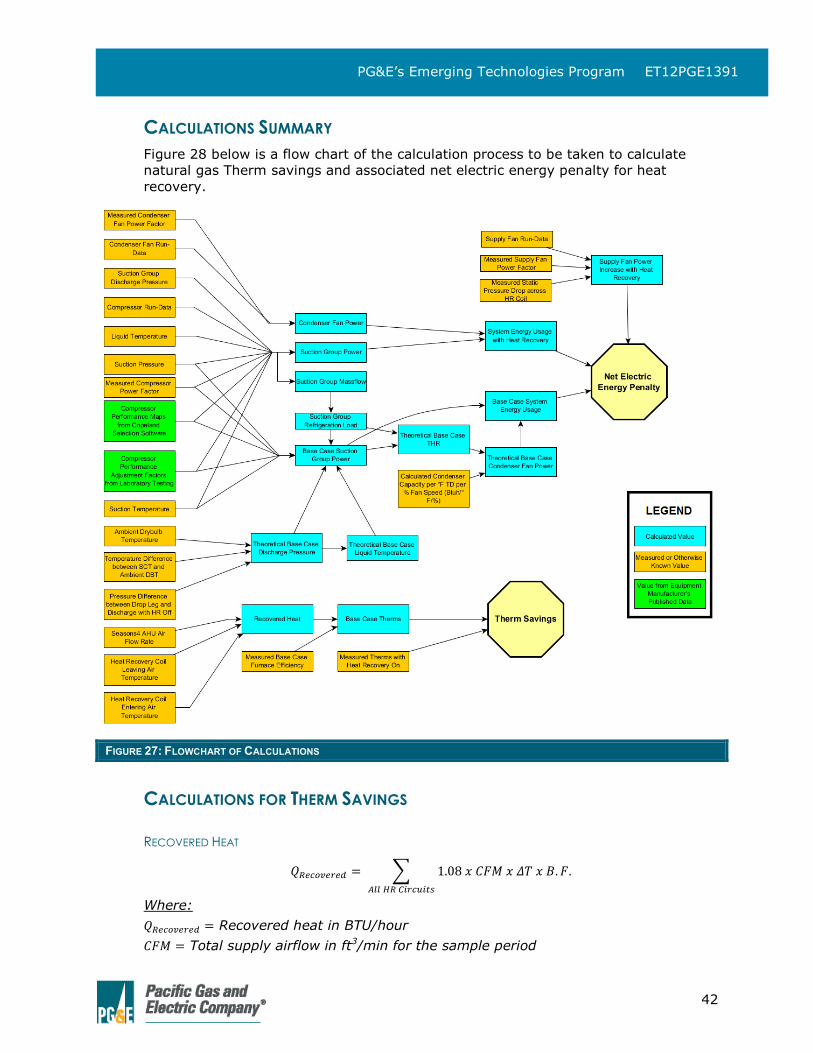
42


CALCULATIONS SUMMARY

Figure 28 below is a flow chart of the calculation process to be taken to calculate

natural gas Therm savings and associated net electric energy penalty for heat

recovery.

FIGURE 27: FLOWCHART OF CALCULATIONS

CALCULATIONS FOR THERM SAVINGS

RECOVERED HEAT

𝑄𝑅𝑒𝑐𝑜𝑣𝑒𝑟𝑒𝑑 = ∑ 1.08 𝑥 𝐶𝐹𝑀 𝑥 𝛥𝑇 𝑥 𝐵. 𝐹.

𝐴𝑙𝑙 𝐻𝑅 𝐶𝑖𝑟𝑐𝑢𝑖𝑡𝑠

Where:

𝑄𝑅𝑒𝑐𝑜𝑣𝑒𝑟𝑒𝑑 = Recovered heat in BTU/hour

𝐶𝐹𝑀 = Total supply airflow in ft3/min for the sample period

43


𝛥𝑇 = Air temperature rise across heat recovery circuit for the sample period

𝐵𝐹 = Airflow % bias factor, found by measuring airflow symmetry at the heat

recovery coil during instrumentation field commissioning

BASE CASE THERMS

𝐵𝑎𝑠𝑒 𝐶𝑎𝑠𝑒 𝑇ℎ𝑒𝑟𝑚𝑠 = 𝑄𝑅𝑒𝑐𝑜𝑣𝑒𝑟𝑒𝑑

𝑒𝑓𝑢𝑟𝑛𝑎𝑐𝑒

Where:

𝑒 = Base Case furnace efficiency, calculated during Base Case performance

establishment period

THERM SAVINGS

𝑇ℎ𝑒𝑟𝑚 𝑆𝑎𝑣𝑖𝑛𝑔𝑠 = 𝐵𝑎𝑠𝑒 𝐶𝑎𝑠𝑒 𝑇ℎ𝑒𝑟𝑚𝑠 − 𝑇ℎ𝑒𝑟𝑚𝑠 𝑤𝑖𝑡ℎ 𝐻𝑒𝑎𝑡 𝑅𝑒𝑐𝑜𝑣𝑒𝑟𝑦

CALCULATIONS FOR NET ELECTRIC ENERGY PENALTY

SUCTION GROUP POWER CALCULATION

𝑃𝑆𝑢𝑐𝑡 𝐺𝑟𝑝 = ∑ (𝑃𝐶𝑜𝑚𝑝 𝑀𝑎𝑝𝑠 𝑥 𝑅𝐹 𝑥 𝑈𝑙𝑑 𝑥 𝑐)

𝐴𝑙𝑙 𝐶𝑜𝑚𝑝𝑠

Where:

𝑃𝑆𝑢𝑐𝑡 𝐺𝑟𝑝 = Total suction group electric power in kW

𝑃𝐶𝑜𝑚𝑝 𝑀𝑎𝑝𝑠 = Compressor power in kW from manufacturer's published performance

maps4

𝑅𝐹 = % compressor run fraction for the sample period

𝑈𝑙𝑑 = % compressor unloader fraction for sample period5

4 Performance Map is a table of compressor massflow and power for varying saturated

suction temperatures and saturated discharge temperatures. See Appendix B for sample

compressor performance maps.

5 The lead compressors of two of the suction groups have digital unloaders, which can

rapidly cycle the compressor pumping capacity off and on, allowing the suction groups to

more precisely match the attached load by modulating the “pulse-width” of the lead

compressor pumping capacity. The compressor unloader fraction is only relevant for

calculating the lead compressor power and massflow.

44


𝑐 = % adjustment factor, derived from comparing published compressor power data

to the power measured during instrumentation field commissioning

SUCTION GROUP MASSFLOW CALCULATION

ṁ𝑆𝑢𝑐𝑡 𝐺𝑟𝑝 = ∑ (ṁ𝐶𝑜𝑚𝑝 𝑀𝑎𝑝𝑠 𝑥 𝑅𝐹 𝑥 𝑈𝑙𝑑 𝑥 𝑐 𝑥 𝑆𝑇𝐴𝐹)

𝐴𝑙𝑙 𝐶𝑜𝑚𝑝𝑠

Where:

ṁ𝑆𝑢𝑐𝑡 𝐺𝑟𝑝 = Total suction group refrigerant massflow in lb./Hr

ṁ𝐶𝑜𝑚𝑝 𝑀𝑎𝑝𝑠 = Compressor refrigerant massflow in lb./Hr from manufacturer's

published performance maps

𝑅𝐹 = % compressor run fraction for sample period

𝑈𝑙𝑑 = % compressor unloader fraction for sample period

𝑐 = % adjustment factor, derived from comparing published data to measured power

𝑆𝑇𝐴𝐹 = Suction Temperature Adjustment Factor, a factor applied to published

compressor capacity ratings, based on laboratory testing of compressor massflow at

varying return gas temperatures. This parameter is variable based on the average

suction temperature for the sample period

SUCTION GROUP LOAD CALCULATION

𝑄𝑆𝑢𝑐𝑡 𝐺𝑟𝑝 = ṁ𝑆𝑢𝑐𝑡 𝐺𝑟𝑝(ℎ𝑣𝑎𝑝𝑜𝑟 − ℎ𝑙𝑖𝑞𝑢𝑖𝑑)

Where:

𝑄𝑆𝑢𝑐𝑡 𝐺𝑟𝑝 = Total suction group refrigeration load in BTU/Hr for the sample period

ṁ𝑆𝑢𝑐𝑡 𝐺𝑟𝑝 = Compressor refrigerant massflow in lb./Hr

ℎ𝑣𝑎𝑝𝑜𝑟 = Enthalpy of refrigerant vapor entering the suction group suction header,

calculated from saturated suction pressure, return gas temperature, and refrigerant

thermodynamic properties

ℎ𝑙𝑖𝑞𝑢𝑖𝑑 = Enthalpy of refrigerant liquid supplied to refrigeration loads, calculated from

dropleg pressure, a one-time measurement of condenser liquid subcooling taken

during instrumentation field commissioning, and refrigerant thermodynamic

properties for Medium Temperature suction groups, and a one-time measurement of

liquid subcooling and refrigerant thermodynamic properties for Low Temperature

suction groups

THEORETICAL BASE CASE DISCHARGE PRESSURE

𝑃𝑡ℎ𝑒𝑜𝑟𝑒𝑡𝑖𝑐𝑎𝑙 = [Refrigerant saturation pressure at [𝑇𝑎𝑚𝑏𝑖𝑒𝑛𝑡 + 𝛥𝑇]] + 𝛥𝑃𝑑𝑖𝑠𝑐ℎ𝑎𝑟𝑔𝑒 𝑐𝑖𝑟𝑐𝑢𝑖𝑡

Where:

𝑇𝑎𝑚𝑏𝑖𝑒𝑛𝑡 = Ambient drybulb temperature, measured at the condenser air inlet for each

refrigeration system for the sample period

45


𝛥𝑇 = Temperature difference between saturated condensing temperature (SCT,

based on pressure measured at condenser dropleg) and ambient drybulb

temperature for the sample period

𝛥𝑃𝑑𝑖𝑠𝑐ℎ𝑎𝑟𝑔𝑒 𝑐𝑖𝑟𝑐𝑢𝑖𝑡 = Pressure drop between compressor discharge pressure and dropleg

pressure, taken from data collected during the Base Case performance establishment

period

THEORETICAL BASE CASE LIQUID TEMPERATURE

For MT Systems:

𝑇𝑙𝑖𝑞𝑢𝑖𝑑,𝑡ℎ𝑒𝑜𝑟𝑒𝑡𝑖𝑐𝑎𝑙 = [saturation temperature at theoretical Base Case disch. P] − 𝑇𝑎𝑚𝑏.𝑆𝐶

For LT Systems:

𝑇𝑙𝑖𝑞𝑢𝑖𝑑,𝑡ℎ𝑒𝑜𝑟𝑒𝑡𝑖𝑐𝑎𝑙 = 𝑆𝑢𝑏𝑐𝑜𝑜𝑙𝑒𝑟 𝑡𝑒𝑚𝑝𝑒𝑟𝑎𝑡𝑢𝑟𝑒 𝑠𝑒𝑡𝑝𝑜𝑖𝑛𝑡

Where:

𝑇𝑎𝑚𝑏.𝑆𝐶 = Ambient subcooling, measured during instrumentation field commissioning.

Ambient subcooling is the difference between the refrigerant saturation temperature

at the dropleg pressure transducer and the actual liquid temperature.

BASE CASE SUCTION GROUP POWER CALCULATION

Base Case suction group power will be derived from the same measured suction

pressure, suction temperature, and compressor maps used to calculate the suction

group power in the Heat Recovery scenario, but the calculation will be based on the

refrigeration load, and the theoretical Base Case discharge pressure instead of the

actual discharge pressure for the sample period. The EnergyDashboard software will

automatically calculate the required lead compressor unloader pulse-width

percentage, and will select the mix of compressors necessary to satisfy the load

based on the programmed compressor sequence for each suction group.

THEORETICAL BASE CASE TOTAL HEAT OF REJECTION (THR)

𝑇𝐻𝑅𝐵𝑎𝑠𝑒𝐶𝑎𝑠𝑒 = 𝑅𝑒𝑓𝑔. 𝐿𝑜𝑎𝑑 + 𝐵𝑎𝑠𝑒 𝐶𝑎𝑠𝑒 𝑆𝑢𝑐𝑡. 𝐺𝑟𝑝 𝑃𝑤𝑟 𝑥 3413

Where:

𝑅𝑒𝑓𝑔. 𝐿𝑜𝑎𝑑 = Calculated refrigeration load in BTU/hour for the sample period

𝐵𝑎𝑠𝑒 𝐶𝑎𝑠𝑒 𝑆𝑢𝑐𝑡. 𝐺𝑟𝑝 𝑃𝑜𝑤𝑒𝑟 = Calculated theoretical Base Case suction group power for

the sample period, in kW

THEORETICAL BASE CASE CONDENSER FAN POWER

The theoretical Base Case condenser fan power will be calculated in four steps:

1. Determine the fraction of condenser capacity required to meet the theoretical Base

Case Total Heat of Rejection

46


𝐶𝑎𝑝𝑎𝑐𝑖𝑡𝑦 𝐹𝑟𝑎𝑐𝑡𝑖𝑜𝑛 = 𝑇𝐻𝑅𝐵𝑎𝑠𝑒𝐶𝑎𝑠𝑒

𝐶𝑜𝑛𝑑𝑒𝑛𝑠𝑒𝑟 𝐶𝑎𝑝𝑎𝑐𝑖𝑡𝑦 𝑎𝑡 100% 𝐹𝑎𝑛 𝑆𝑝𝑒𝑒𝑑 𝑎𝑡 𝐴𝑝𝑝𝑙𝑖𝑒𝑑 𝑇𝐷

Where the Condenser Capacity at 100% Fan Speed at the Applied TD is the capacity

per °F TD which was determined in the Base Case performance establishment period,

multiplied by the temperature difference between the SCT and the ambient drybulb

temperature

2. Determine the theoretical Base Case condenser % fan speed. The fan speed is the

independent variable in the following equation, which is based on laboratory testing

of an air-cooled condenser:

𝐶𝑜𝑛𝑑𝑒𝑛𝑠𝑒𝑟 𝐶𝑎𝑝𝑎𝑐𝑖𝑡𝑦 % = 0.196𝑥3 − 0.7239𝑥2 + 1.5329𝑥 − 0.0002

The independent variable in a third-order polynomial can be determined with the

following equation:

Where, for this analysis:

a = 0.196

b = -0.7239

c = 1.5329

d = -0.0002

3. Calculate % fan power from % fan speed. % fan power is the dependent variable in

the following equation, which is based on laboratory testing of an air-cooled

condenser:

% 𝐹𝑎𝑛 𝑃𝑜𝑤𝑒𝑟 = 2.317𝑥3 − 2.543𝑥2 + 1.4568𝑥 − 0.238

(Coefficients are irrational numbers—only four significant digits are shown, but the

actual calculation will include as many significant figures as the EnergyDashboard

calculation tool will allow)

4. Calculate fan power

𝑃𝑐𝑜𝑛𝑑 𝑓𝑎𝑛 = % 𝐹𝑎𝑛 𝑃𝑜𝑤𝑒𝑟 𝑥 𝑀𝑒𝑎𝑠𝑢𝑟𝑒𝑑 𝐹𝑎𝑛 𝑃𝑜𝑤𝑒𝑟 𝑎𝑡 100% 𝑆𝑝𝑒𝑒𝑑 𝑓𝑟𝑜𝑚 𝐶𝑜𝑚𝑚𝑖𝑠𝑠𝑖𝑜𝑛𝑖𝑛𝑔

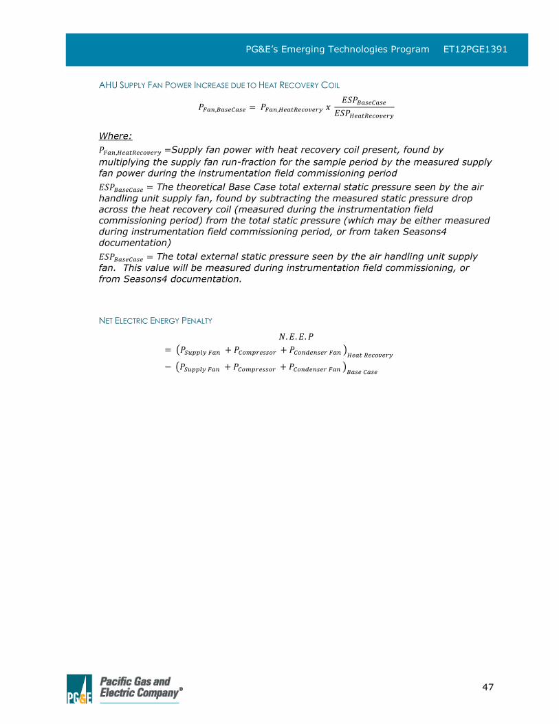
47


AHU SUPPLY FAN POWER INCREASE DUE TO HEAT RECOVERY COIL

𝑃𝐹𝑎𝑛,𝐵𝑎𝑠𝑒𝐶𝑎𝑠𝑒 = 𝑃𝐹𝑎𝑛,𝐻𝑒𝑎𝑡𝑅𝑒𝑐𝑜𝑣𝑒𝑟𝑦 𝑥 𝐸𝑆𝑃𝐵𝑎𝑠𝑒𝐶𝑎𝑠𝑒

𝐸𝑆𝑃𝐻𝑒𝑎𝑡𝑅𝑒𝑐𝑜𝑣𝑒𝑟𝑦

Where:

𝑃𝐹𝑎𝑛,𝐻𝑒𝑎𝑡𝑅𝑒𝑐𝑜𝑣𝑒𝑟𝑦 =Supply fan power with heat recovery coil present, found by

multiplying the supply fan run-fraction for the sample period by the measured supply

fan power during the instrumentation field commissioning period

𝐸𝑆𝑃𝐵𝑎𝑠𝑒𝐶𝑎𝑠𝑒 = The theoretical Base Case total external static pressure seen by the air

handling unit supply fan, found by subtracting the measured static pressure drop

across the heat recovery coil (measured during the instrumentation field

commissioning period) from the total static pressure (which may be either measured

during instrumentation field commissioning period, or from taken Seasons4

documentation)

𝐸𝑆𝑃𝐵𝑎𝑠𝑒𝐶𝑎𝑠𝑒 = The total external static pressure seen by the air handling unit supply

fan. This value will be measured during instrumentation field commissioning, or

from Seasons4 documentation.

NET ELECTRIC ENERGY PENALTY

𝑁. 𝐸. 𝐸. 𝑃

= (𝑃𝑆𝑢𝑝𝑝𝑙𝑦 𝐹𝑎𝑛 + 𝑃𝐶𝑜𝑚𝑝𝑟𝑒𝑠𝑠𝑜𝑟 + 𝑃𝐶𝑜𝑛𝑑𝑒𝑛𝑠𝑒𝑟 𝐹𝑎𝑛 )𝐻𝑒𝑎𝑡 𝑅𝑒𝑐𝑜𝑣𝑒𝑟𝑦

− (𝑃𝑆𝑢𝑝𝑝𝑙𝑦 𝐹𝑎𝑛 + 𝑃𝐶𝑜𝑚𝑝𝑟𝑒𝑠𝑠𝑜𝑟 + 𝑃𝐶𝑜𝑛𝑑𝑒𝑛𝑠𝑒𝑟 𝐹𝑎𝑛 )𝐵𝑎𝑠𝑒 𝐶𝑎𝑠𝑒

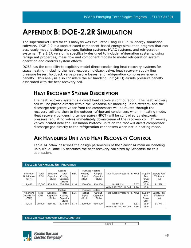
48


APPENDIX B: DOE-2.2R SIMULATION The supermarket used for this analysis was evaluated using DOE-2.2R energy simulation

software. DOE-2.2 is a sophisticated component-based energy simulation program that can

accurately model building envelope, lighting systems, HVAC systems, and refrigeration

systems. The 2.2R version is specifically designed to include refrigeration systems, using

refrigerant properties, mass flow and component models to model refrigeration system

operation and controls system effects.

DOE2 has the capability to explicitly model direct-condensing heat recovery systems for

space heating, including the heat recovery holdback valve, heat recovery supply line

pressure losses, holdback valve pressure losses, and refrigeration compressor energy

penalty. This analysis also considers the air handling unit (AHU) airside pressure penalty

associated with the heat recovery coil.

HEAT RECOVERY SYSTEM DESCRIPTION The heat recovery system is a direct heat recovery configuration. The heat recovery

coil will be placed directly within the Seasons4 air handling unit airstream, and the

discharge refrigerant vapor from the compressors will be routed through the

recovery coil and then to the outdoor refrigerant condensers when in heating mode.

Heat recovery condensing temperature (HRCT) will be controlled by electronic

pressure regulating valves immediately downstream of the recovery coil. Three-way

valves located near the Hussmann Protocol units on the roof will divert compressor

discharge gas directly to the refrigeration condensers when not in heating mode.

AIR HANDLING UNIT AND HEAT RECOVERY CONTROL Table 14 below describes the design parameters of the Seasons4 main air handling

unit, while Table 15 describes the heat recovery coil sized by Seasons4 for this

application.

TABLE 23: AIR HANDLING UNIT PROPERTIES

Cooling Furnace Heating

Minimum

Outside Air

(CFM)

Total

CFM

Sensible

Capacity

(Btuh)

Total

Cooling

Capacity

(Btuh)

EER Heating

Input

(Btuh)

Output

Capacity

(Btuh)

Total Static Pressure (in. WC) Supply

Fan

Power

(BHP)

Supply Fan

Efficiency

(%)

9,420 20,000 439,313 524,884 11.4 1,200,000 960,000 No HR Coil 3.67 15.9 91.7%

With 0.49" WC HR Coil 4.16 18.0

Cooling Furnace Heating

Minimum

Outside Air

(CFM)

Total

CFM

Sensible

Capacity

(Btuh)

Total

Cooling

Capacity

(Btuh)

EER Heating

Input

(Btuh)

Output

Capacity

(Btuh)

Total Static Pressure (in. WC) Supply

Fan

Power

(BHP)

Supply Fan

Efficiency

(%)

9,420 20,000 439,313 524,884 11.4 1,200,000 960,000 No HR Coil 3.67 15.9 91.7%

With 0.49" WC HR Coil 4.16 18.0

TABLE 24: HEAT RECOVERY COIL PARAMETERS

Rows 4

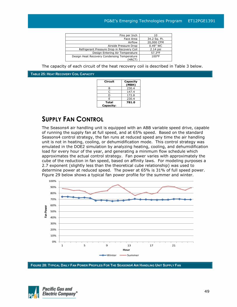
49


Fins per Inch 10

Face Area 34.2 Sq. Ft.

Airflow 20,000 CFM

Airside Pressure Drop 0.49” WC

Refrigerant Pressure Drop in Recovery Coil 2.14 psi

Design Entering Air Temperature 57.3°F

Design Heat Recovery Condensing Temperature (HRCT)

100°F

The capacity of each circuit of the heat recovery coil is described in Table 3 below.

TABLE 25: HEAT RECOVERY COIL CAPACITY

Circuit Capacity

(MBH)

B 230.4

C 147.4

D 172.8

E 230.4

Total Capacity:

781.0

SUPPLY FAN CONTROL The Seasons4 air handling unit is equipped with an ABB variable speed drive, capable

of running the supply fan at full speed, and at 65% speed. Based on the standard

Seasons4 control strategy, the fan runs at reduced speed any time the air handling

unit is not in heating, cooling, or dehumidification mode. This control strategy was

emulated in the DOE2 simulation by analyzing heating, cooling, and dehumidification

load for every hour of the year, and generating a minimum flow schedule which

approximates the actual control strategy. Fan power varies with approximately the

cube of the reduction in fan speed, based on affinity laws. For modeling purposes a

2.7 exponent (slightly less than the theoretical cube relationship) was used to

determine power at reduced speed. The power at 65% is 31% of full speed power.

Figure 29 below shows a typical fan power profile for the summer and winter.

FIGURE 28: TYPICAL DAILY FAN POWER PROFILES FOR THE SEASONS4 AIR HANDLING UNIT SUPPLY FAN

0%

10%

20%

30%

40%

50%

60%

70%

80%

90%

100%

1 5 9 13 17 21

Fan

Pow

er

Hour

Winter Summer

50


The analysis model incorporated the current Seasons4 fan control logic, which only

reduces fan speed in the “deadband” when there is no heating or cooling. This

strategy could be improved, and in fact, may not be compliant with the intent of the

new Title 24 fan speed requirements for packaged HVAC units. A more advanced

strategy with speed control based on the demand for heating and cooling may

provide considerable additional fan savings and reduced pressure drop penalty at the

heat recovery coil (likely enough to completely offset the heat recovery electric

energy penalty) as well as providing improved latent cooling performance. This

opportunity should be considered for additional savings and as a possibly component

of future heat recovery integration, but in order to reduce the number of study

variables, only implemented after the benefit of heat recovery by itself has been

determined.

HOLDBACK VALVE CONTROL Sporlan model CDS electronic pressure regulating valves will be used for the heat

recovery holdback valves, and will be controlled to a recovery condensing pressure

setpoint. The control parameter will be the heat recovery condensing temperature

(HRCT) setpoint. The target HRCT in the heat recovery coil circuit will be set at a

value determined by adding the actual mixed return/outside air temperature in the

Seasons4 unit and a preset temperature difference value (assumed to be 20°F for

this analysis).

This variable HRCT setpoint will also be bounded by a maximum HRCT setpoint of

95°F and a minimum HRCT setpoint, which will be determined from the operating

saturated condensing temperature (SCT) at the refrigeration condenser plus a preset

temperature difference, e.g. 10°F. The latter value will insure there will always be

pressure drop across the heat recovery holdback valve and resulting flash gas to

maintain a reasonable velocity in the heat recovery piping and condenser; which

serves the purpose of avoiding excessive charge in the condenser and piping during

heat recovery.

The DOE2 TEMP-RESET scheduling capability was utilized to simulate the proposed

electronic holdback valve control. The TEMP-RESET schedule correlates a

temperature control parameter (HRCT setpoint in this case) to entering air

temperature using a linear relationship, with user-selectable maximums and

minimums. Figure 30 below shows the average HRCT setpoint for each month.

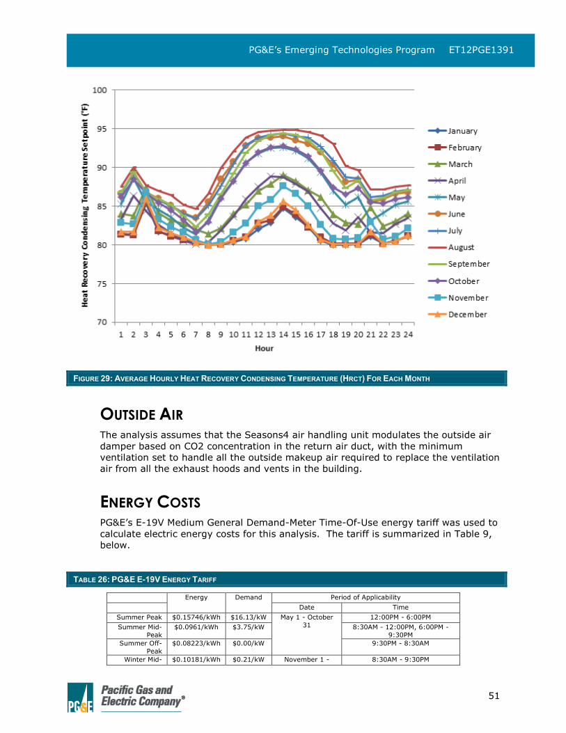
51


FIGURE 29: AVERAGE HOURLY HEAT RECOVERY CONDENSING TEMPERATURE (HRCT) FOR EACH MONTH

OUTSIDE AIR The analysis assumes that the Seasons4 air handling unit modulates the outside air

damper based on CO2 concentration in the return air duct, with the minimum

ventilation set to handle all the outside makeup air required to replace the ventilation

air from all the exhaust hoods and vents in the building.

ENERGY COSTS PG&E’s E-19V Medium General Demand-Meter Time-Of-Use energy tariff was used to

calculate electric energy costs for this analysis. The tariff is summarized in Table 9,

below.

TABLE 26: PG&E E-19V ENERGY TARIFF

Energy Demand Period of Applicability

Date Time

Summer Peak $0.15746/kWh $16.13/kW May 1 - October

31

12:00PM - 6:00PM

Summer Mid-

Peak

$0.0961/kWh $3.75/kW 8:30AM - 12:00PM, 6:00PM -

9:30PM

Summer Off-

Peak

$0.08223/kWh $0.00/kW 9:30PM - 8:30AM

Winter Mid- $0.10181/kWh $0.21/kW November 1 - 8:30AM - 9:30PM

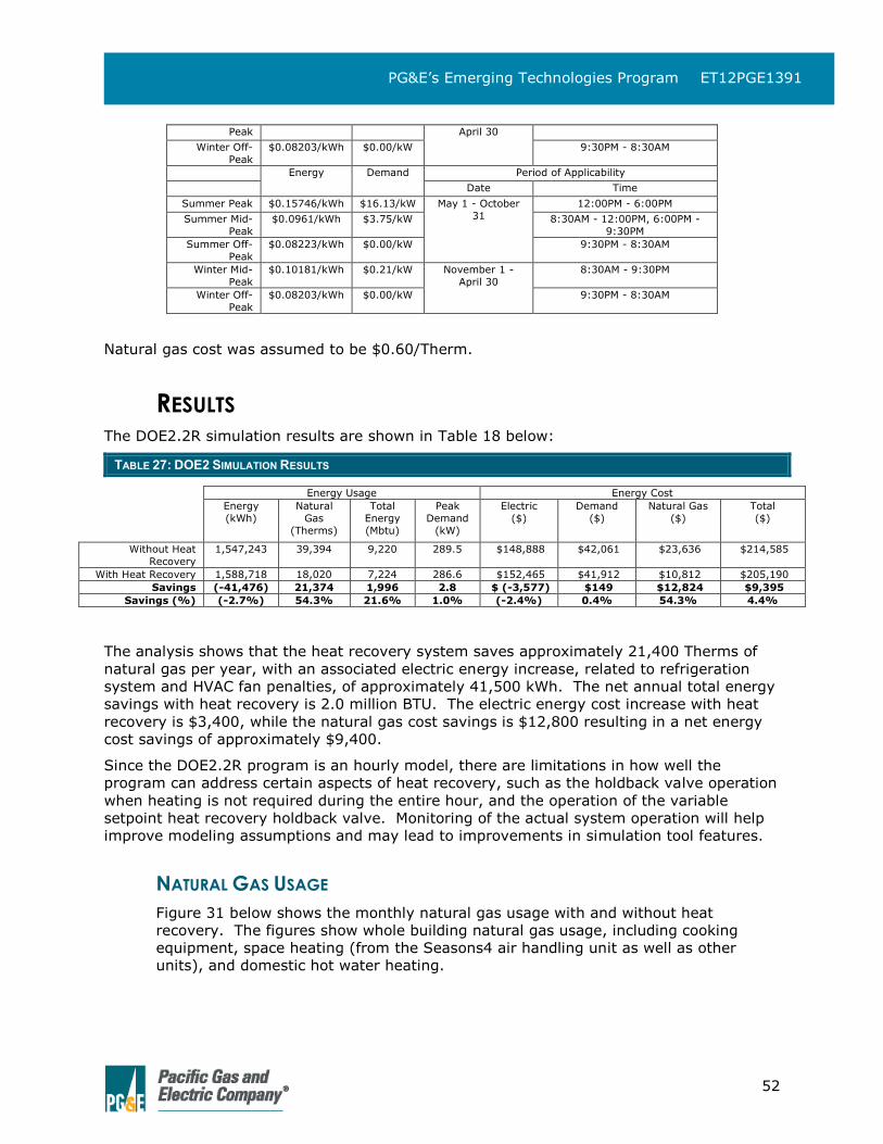
52


Peak April 30

Winter Off-

Peak

$0.08203/kWh $0.00/kW 9:30PM - 8:30AM

Energy Demand Period of Applicability

Date Time

Summer Peak $0.15746/kWh $16.13/kW May 1 - October

31

12:00PM - 6:00PM

Summer Mid-

Peak

$0.0961/kWh $3.75/kW 8:30AM - 12:00PM, 6:00PM -

9:30PM

Summer Off-

Peak

$0.08223/kWh $0.00/kW 9:30PM - 8:30AM

Winter Mid-

Peak

$0.10181/kWh $0.21/kW November 1 -

April 30

8:30AM - 9:30PM

Winter Off-

Peak

$0.08203/kWh $0.00/kW 9:30PM - 8:30AM

Natural gas cost was assumed to be $0.60/Therm.

RESULTS The DOE2.2R simulation results are shown in Table 18 below:

TABLE 27: DOE2 SIMULATION RESULTS

Energy Usage Energy Cost

Energy

(kWh)

Natural

Gas

(Therms)

Total

Energy

(Mbtu)

Peak

Demand

(kW)

Electric

($)

Demand

($)

Natural Gas

($)

Total

($)

Without Heat

Recovery

1,547,243 39,394 9,220 289.5 $148,888 $42,061 $23,636 $214,585

With Heat Recovery 1,588,718 18,020 7,224 286.6 $152,465 $41,912 $10,812 $205,190

Savings (-41,476) 21,374 1,996 2.8 $ (-3,577) $149 $12,824 $9,395

Savings (%) (-2.7%) 54.3% 21.6% 1.0% (-2.4%) 0.4% 54.3% 4.4%

The analysis shows that the heat recovery system saves approximately 21,400 Therms of

natural gas per year, with an associated electric energy increase, related to refrigeration

system and HVAC fan penalties, of approximately 41,500 kWh. The net annual total energy

savings with heat recovery is 2.0 million BTU. The electric energy cost increase with heat

recovery is $3,400, while the natural gas cost savings is $12,800 resulting in a net energy

cost savings of approximately $9,400.

Since the DOE2.2R program is an hourly model, there are limitations in how well the

program can address certain aspects of heat recovery, such as the holdback valve operation

when heating is not required during the entire hour, and the operation of the variable

setpoint heat recovery holdback valve. Monitoring of the actual system operation will help

improve modeling assumptions and may lead to improvements in simulation tool features.

NATURAL GAS USAGE

Figure 31 below shows the monthly natural gas usage with and without heat

recovery. The figures show whole building natural gas usage, including cooking

equipment, space heating (from the Seasons4 air handling unit as well as other

units), and domestic hot water heating.

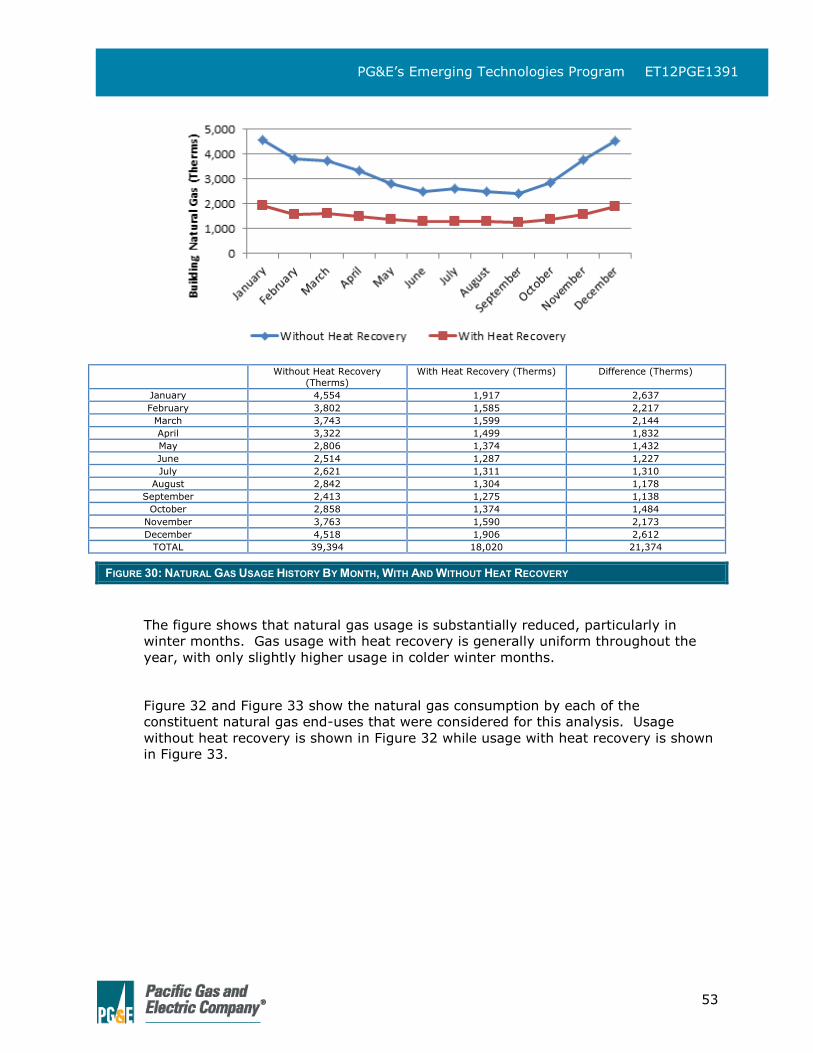
53


Without Heat Recovery

(Therms)

With Heat Recovery (Therms) Difference (Therms)

January 4,554 1,917 2,637

February 3,802 1,585 2,217

March 3,743 1,599 2,144

April 3,322 1,499 1,832

May 2,806 1,374 1,432

June 2,514 1,287 1,227

July 2,621 1,311 1,310

August 2,842 1,304 1,178

September 2,413 1,275 1,138

October 2,858 1,374 1,484

November 3,763 1,590 2,173

December 4,518 1,906 2,612

TOTAL 39,394 18,020 21,374

FIGURE 30: NATURAL GAS USAGE HISTORY BY MONTH, WITH AND WITHOUT HEAT RECOVERY

The figure shows that natural gas usage is substantially reduced, particularly in

winter months. Gas usage with heat recovery is generally uniform throughout the

year, with only slightly higher usage in colder winter months.

Figure 32 and Figure 33 show the natural gas consumption by each of the

constituent natural gas end-uses that were considered for this analysis. Usage

without heat recovery is shown in Figure 32 while usage with heat recovery is shown

in Figure 33.

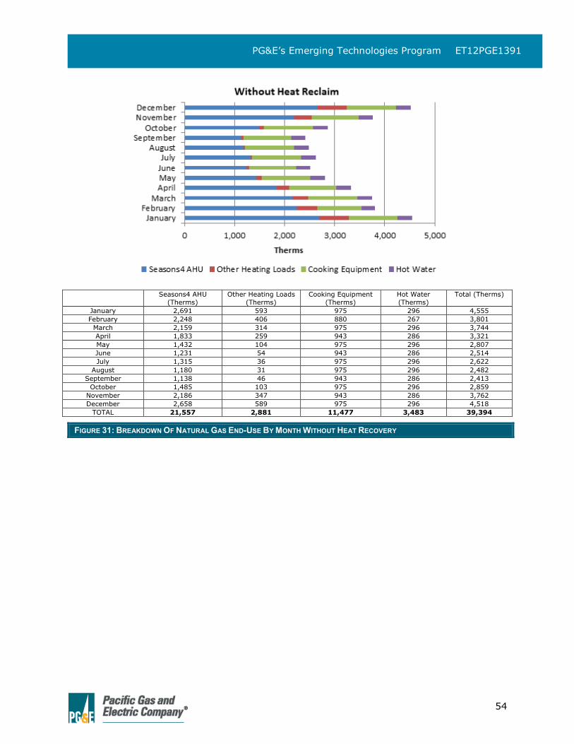
54


Seasons4 AHU

(Therms)

Other Heating Loads

(Therms)

Cooking Equipment

(Therms)

Hot Water

(Therms)

Total (Therms)

January 2,691 593 975 296 4,555

February 2,248 406 880 267 3,801

March 2,159 314 975 296 3,744

April 1,833 259 943 286 3,321

May 1,432 104 975 296 2,807

June 1,231 54 943 286 2,514

July 1,315 36 975 296 2,622

August 1,180 31 975 296 2,482

September 1,138 46 943 286 2,413

October 1,485 103 975 296 2,859

November 2,186 347 943 286 3,762

December 2,658 589 975 296 4,518

TOTAL 21,557 2,881 11,477 3,483 39,394

FIGURE 31: BREAKDOWN OF NATURAL GAS END-USE BY MONTH WITHOUT HEAT RECOVERY

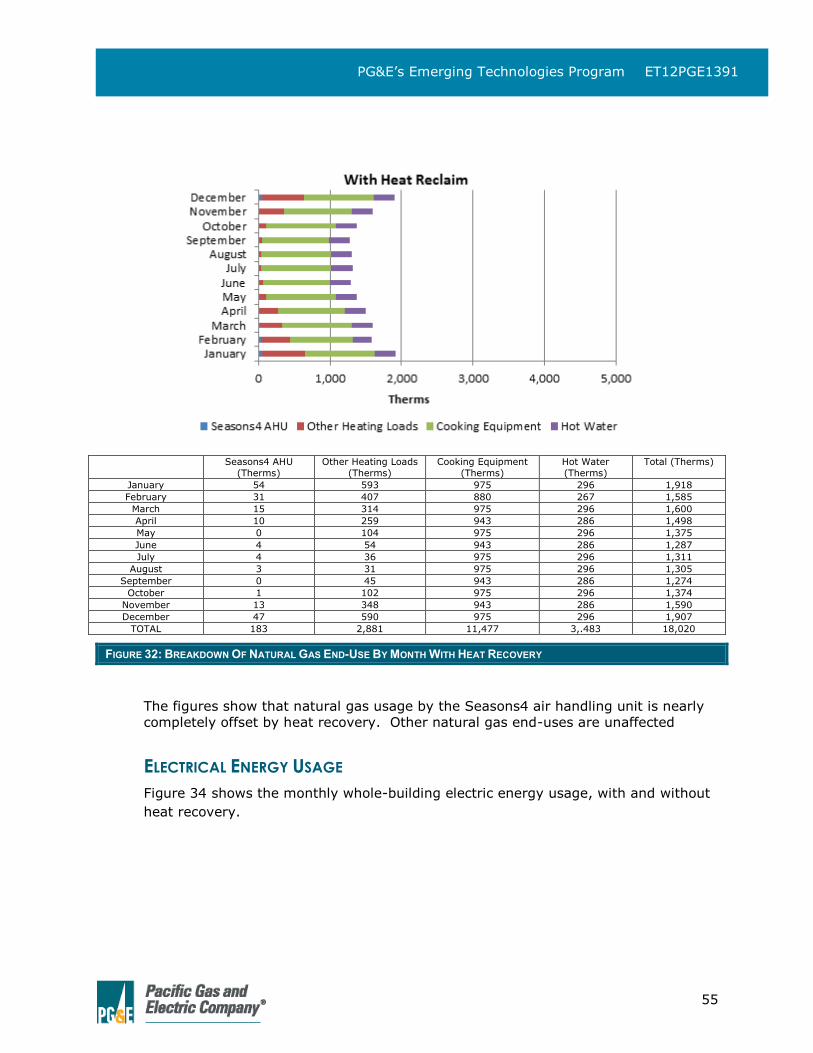
55


Seasons4 AHU

(Therms)

Other Heating Loads

(Therms)

Cooking Equipment

(Therms)

Hot Water

(Therms)

Total (Therms)

January 54 593 975 296 1,918

February 31 407 880 267 1,585

March 15 314 975 296 1,600

April 10 259 943 286 1,498

May 0 104 975 296 1,375

June 4 54 943 286 1,287

July 4 36 975 296 1,311

August 3 31 975 296 1,305

September 0 45 943 286 1,274

October 1 102 975 296 1,374

November 13 348 943 286 1,590

December 47 590 975 296 1,907

TOTAL 183 2,881 11,477 3,.483 18,020

FIGURE 32: BREAKDOWN OF NATURAL GAS END-USE BY MONTH WITH HEAT RECOVERY

The figures show that natural gas usage by the Seasons4 air handling unit is nearly

completely offset by heat recovery. Other natural gas end-uses are unaffected

ELECTRICAL ENERGY USAGE

Figure 34 shows the monthly whole-building electric energy usage, with and without

heat recovery.

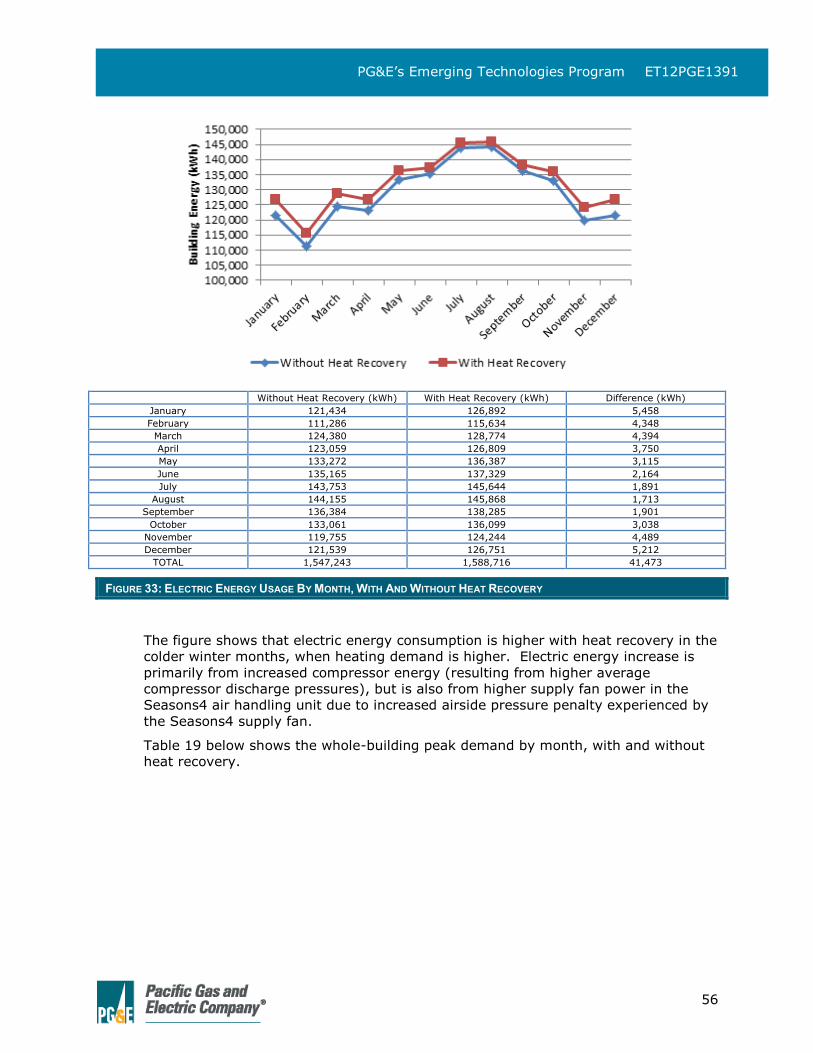
56


Without Heat Recovery (kWh) With Heat Recovery (kWh) Difference (kWh)

January 121,434 126,892 5,458

February 111,286 115,634 4,348

March 124,380 128,774 4,394

April 123,059 126,809 3,750

May 133,272 136,387 3,115

June 135,165 137,329 2,164

July 143,753 145,644 1,891

August 144,155 145,868 1,713

September 136,384 138,285 1,901

October 133,061 136,099 3,038

November 119,755 124,244 4,489

December 121,539 126,751 5,212

TOTAL 1,547,243 1,588,716 41,473

FIGURE 33: ELECTRIC ENERGY USAGE BY MONTH, WITH AND WITHOUT HEAT RECOVERY

The figure shows that electric energy consumption is higher with heat recovery in the

colder winter months, when heating demand is higher. Electric energy increase is

primarily from increased compressor energy (resulting from higher average

compressor discharge pressures), but is also from higher supply fan power in the

Seasons4 air handling unit due to increased airside pressure penalty experienced by

the Seasons4 supply fan.

Table 19 below shows the whole-building peak demand by month, with and without

heat recovery.

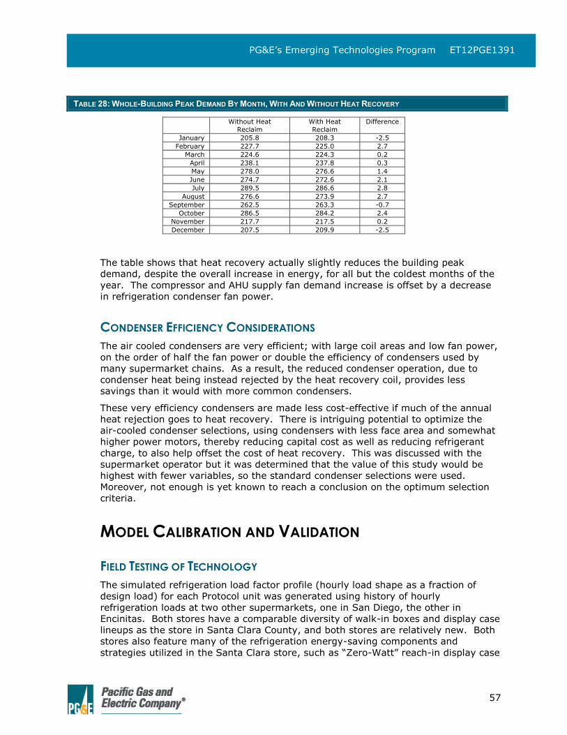
57


TABLE 28: WHOLE-BUILDING PEAK DEMAND BY MONTH, WITH AND WITHOUT HEAT RECOVERY

Without Heat

Reclaim

With Heat

Reclaim

Difference

January 205.8 208.3 -2.5

February 227.7 225.0 2.7

March 224.6 224.3 0.2

April 238.1 237.8 0.3

May 278.0 276.6 1.4

June 274.7 272.6 2.1

July 289.5 286.6 2.8

August 276.6 273.9 2.7

September 262.5 263.3 -0.7

October 286.5 284.2 2.4

November 217.7 217.5 0.2

December 207.5 209.9 -2.5

The table shows that heat recovery actually slightly reduces the building peak

demand, despite the overall increase in energy, for all but the coldest months of the

year. The compressor and AHU supply fan demand increase is offset by a decrease

in refrigeration condenser fan power.

CONDENSER EFFICIENCY CONSIDERATIONS

The air cooled condensers are very efficient; with large coil areas and low fan power,

on the order of half the fan power or double the efficiency of condensers used by

many supermarket chains. As a result, the reduced condenser operation, due to

condenser heat being instead rejected by the heat recovery coil, provides less

savings than it would with more common condensers.

These very efficiency condensers are made less cost-effective if much of the annual

heat rejection goes to heat recovery. There is intriguing potential to optimize the

air-cooled condenser selections, using condensers with less face area and somewhat

higher power motors, thereby reducing capital cost as well as reducing refrigerant

charge, to also help offset the cost of heat recovery. This was discussed with the

supermarket operator but it was determined that the value of this study would be

highest with fewer variables, so the standard condenser selections were used.

Moreover, not enough is yet known to reach a conclusion on the optimum selection

criteria.

MODEL CALIBRATION AND VALIDATION

FIELD TESTING OF TECHNOLOGY

The simulated refrigeration load factor profile (hourly load shape as a fraction of

design load) for each Protocol unit was generated using history of hourly

refrigeration loads at two other supermarkets, one in San Diego, the other in

Encinitas. Both stores have a comparable diversity of walk-in boxes and display case

lineups as the store in Santa Clara County, and both stores are relatively new. Both

stores also feature many of the refrigeration energy-saving components and

strategies utilized in the Santa Clara store, such as “Zero-Watt” reach-in display case

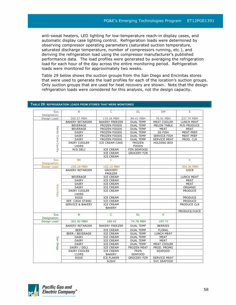
58


anti-sweat heaters, LED lighting for low-temperature reach-in display cases, and

automatic display case lighting control. Refrigeration loads were determined by

observing compressor operating parameters (saturated suction temperature,

saturated discharge temperature, number of compressors running, etc.), and

deriving the refrigeration load using the compressor manufacturer’s published

performance data. The load profiles were generated by averaging the refrigeration

load for each hour of the day across the entire monitoring period. Refrigeration

loads were monitored for approximately two weeks.

Table 29 below shows the suction groups from the San Diego and Encinitas stores

that were used to generate the load profiles for each of the location’s suction groups.

Only suction groups that are used for heat recovery are shown. Note that the design

refrigeration loads were considered for this analysis, not the design capacity.

TABLE 29: REFRIGERATION LOADS FROM STORES THAT WERE MONITORED

Sys.

Designation:

B C DL DM E

Design Load: 260.57 MBH 119.36 MBH 84.41 MBH 76.91 MBH 237.74 MBH

Santa

Cla

ra C

ounty

BAKERY RETARDER BAKERY FREEZER DUAL TEMP MEAT COOLER LUNCH MEAT

BEVERAGE FROZEN FOODS DUAL TEMP MELON TABLE M/D PRODUCE

BEVERAGE FROZEN FOODS DUAL TEMP MEAT MEAT

DAIRY FROZEN FOODS DUAL TEMP SS FISH MEAT PREP

DAIRY FROZEN FOODS DUAL TEMP SERVICE FISH MEAT PREP

DAIRY FROZEN FOODS DUAL TEMP SERVICE MEAT PROD. CLR

DAIRY COOLER 14DRS

ICE CREAM CAKE FROZEN FOODS

HOLDING BOX

M/D DELI ICE CREAM FZN SEAFOOD

ICE CREAM GROCERY FZR

ICE CREAM

Sys.

Designation:

BR C E

Design Load: 236.18 MBH 152.10 MBH 304.36 MBH

Encin

itas

BAKERY RETARDER GROCERY

FREEZER

JUICE

BEVERAGE ICE CREAM LUNCH MEAT

DAIRY ICE CREAM MEAT

DAIRY ICE CREAM MEAT

DAIRY ICE CREAM ORGANIC

DAIRY COOLER

14DRS

ICE CREAM PRODUCE

EGGS ICE CREAM PRODUCE

REF. CASH STAND ICE CREAM PRODUCE

SERVICE & BAKERY ICE CREAM

BAKERY

PRODUCE CLR

PRODUCE/JUICE

Sys.

Designation:

B C DL E

Design Load: 301.92 MBH 160.42 74.78 MBH 197.71

San D

iego

BAKERY RETARDER BAKERY FREEZER DUAL TEMP BERRIES

BEER ICE CREAM DUAL TEMP FLORAL

BEER / BEVERAGE ICE CREAM DUAL TEMP LUNCH MEAT

DAIRY ICE CREAM DUAL TEMP MEAT

DAIRY ICE CREAM DUAL TEMP MEAT

DAIRY ICE CREAM DUAL TEMP MEAT COOLER

DAIRY / DELI ICE CREAM FROZEN MEAT PROD. PROMO

DAIRY COOLER

11DRS

ICE CREAM

BAKERY

FRZN

SEAFOOD

SEAFOOD

EGGS ICE FLAKER GROCERY FZR SERVICE MEAT

SUSHI SVC SEAFOOD

59


Figure 36 through Figure 40 show the load profiles for the two stores as well as the

simulated load profile for the Santa Clara store. On average, all suction groups were

observed to be approximately 40%-65% loaded (vs. the design load) during the two-week

monitoring period.

FIGURE 34: LOAD PROFILES FOR SANTA CLARA COUNTY PROTOCOL B, SHOWN WITH COMPARABLE LOADS FROM THE SAN

DIEGO AND ENCINITAS STORES.

0%

10%

20%

30%

40%

50%

60%

70%

1 4 7 10 13 16 19 22

% o

f Des

ign

Load

Hour

Protocol B

Simulation Encinitas San Diego

60


FIGURE 35: LOAD PROFILES FOR SANTA CLARA STORE PROTOCOL C, SHOWN WITH COMPARABLE LOADS FROM THE SAN

DIEGO AND ENCINITAS STORES

FIGURE 36: LOAD PROFILES FOR SANTA CLARA COUNTY PROTOCOL DL, SHOWN WITH COMPARABLE LOADS FROM THE SAN


FIGURE 37: LOAD PROFILES FOR SANTA CLARA COUNTY PROTOCOL DM, SHOWN WITH COMPARABLE LOADS FROM THE

SAN DIEGO AND ENCINITAS STORES

61


FIGURE 38: LOAD PROFILES FOR SANTA CLARA COUNTY PROTOCOL E, SHOWN WITH COMPARABLE LOADS FROM SAN


NATURAL GAS USAGE ANALYSIS

Simulated natural gas usage for the Santa Clara County location energy model

(without heat recovery) was compared to real usage history from supermarkets from

the same chain located in the same climate zone as the subject store. The usage-

histories being compared to 2007-year histories are for a store in Mill Valley,

California, and a store in Soquel, California. The Santa Clara County store energy

model is in-between Mill Valley and Soquel in terms of floor area (53,500 SF versus

43,900 SF for Mill Valley and 67,100 SF for Soquel). Lighting power density for the

Mill Valley (2.24 Watts/SF) and Soquel (1.74 Watts/SF) are higher than Santa Clara

County location (1.04 Watts/SF). Figure 13 below shows the monthly natural gas

usage for the two stores, along with the simulated natural gas usage for the Santa

Clara County store.

62


Month Santa Clara

County

Mill Valley Soquel

January 4,555 5,010 5,139

February 3,801 4,151 5,460

March 3,744 3,862 4,704

April 3,321 2,908 4,229

May 2,807 3,674 4,373

June 2,514 3,683 3,524

July 2,622 2,492 3,000

August 2,482 1,998 2,405

September 2,413 1,755 2,612

October 2,859 2,486 2,287

November 3,762 2,880 4,020

December 4,518 5,471 5,169

FIGURE 39: NATURAL GAS USAGE FOR THE SANTA CLARA COUNTY STORE, COMPARED TO TWO OTHER SUPERMARKETS

The figure shows that the simulated natural gas usage is generally comparable to the

two other stores. The lighting power density at the Santa Clara County location is

lower than Mill Valley and Soquel, which would expectedly increase natural gas

usage. The host site, however, also utilizes heat pumps instead of natural gas

heaters for several secondary heating loads, and also has less display case lighting

and reach-in anti-sweat heater energy. Identify all the variables that will provide the

output performance of each technology/product and power input to the

technology/product so that the efficiency of the technology/product can be

determined.

63


APPENDIX C: BUILDING SUMMARY The supermarket used for this analysis is approximately 54,000 S.F., out of which 53,500

S.F. is refrigerated or conditioned. The main sales area is conditioned by the Season4 air

handling unit. Other areas are conditioned using Trane packaged rooftop units and Fujitsu

heat pumps.

Refrigeration is accomplished by one low-temperature (LT) system, two dual-temperature

(DT) systems and three medium-temperature (MT) systems, which use R-507 refrigerant.

The refrigeration systems consist of six distributed Hussmann Protocol parallel rack

systems, utilizing Copeland scroll compressors. Krack air cooled units work as the

refrigeration condensers. The following tables outline the primary building systems and

components that were considered in the analysis.

For this analysis the store was assumed to be open 24 hours per day, 7 days per week.

ENVELOPE AND LIGHTING POWER Building construction details and lighting power are described in Figure 35 and Figure

36 below.

TABLE 30: ENVELOPE DESCRIPTION

Wall Construction Mass Heavy Wall. U-factor: 0.65

Roof Insulation Wood Framed and Other Roof. U-factor: 0.039

Roof Absorptivity Absorptivity = 0.45

TABLE 31: LIGHTING POWER

Space Area

(SF)

Lighting Power

Density

(Watts/SF)

Total

Power

(Watts)

Sales 38,309 1.04 39,972

Bakery 1,635 1.74 2,840

Pharmacy 288 2.17 625

Deli 1,247 1.84 2,296

Receiving 6,462 0.40 2,578

Produce Prep 288 1.71 492

Offices/Restrooms 2,315 1.26 2,909

Meat Prep 880 2.09 1,836

Total 51,424 1.04 53,547

64


HUSSMANN PROTOCOL REFRIGERATION SYSTEMS The Santa Clara County store uses Hussmann Protocol parallel rack distributed

refrigeration systems. Table 22 below summarizes the design parameters for the

systems.

TABLE 32: HUSSMANN PROTOCOL REFRIGERATION SYSTEM SUMMARY

System

Configuration

Hussmann Protocol single-stage parallel systems with scroll compressors

Design saturated suction temperatures and design loads as follows:

Protocol A

Suction Group AL: -15°F, 11.1 MBH Suction Group AM: +18°F, 198.36 MBH

Protocol B: +24°F, 260.57 MBH

Protocol C: -20°F, 119.36 MBH

Protocol D

Suction Group DL: -23°F, 84.41 MBH

Suction Group DM: +18°F,76.91 MBH

Protocol E: +24°F, 237.74 MBH

Protocol F: +18°F, 39.8 MBH

Compressor

Quantity and Model

Copeland scroll compressors

Protocol A

Suction Group AL: (1) ZF11K4E economized Suction Group AM: (5) ZB45KCE

Protocol B: (6) ZB45KCE

Protocol C: (6) ZF18KVE economized

Protocol D

Suction Group DL: (1) ZFD18KVE economized digital, (3) ZF18KVE economized

Suction Group DM: (1) ZBD45KCE digital, (1) ZB45KCE digital

Protocol E: (6) ZB45KCE

Protocol F: (6) ZB45KCE

Refrigerant R-507

The compressor control strategy includes electronic sequencing and floating suction

pressure logic, allowing the refrigeration system suction pressure to float rather than

operating at a fixed suction setpoint. During low-load periods, the compressors

operate at a higher suction temperature, improving compressor pumping efficiency,

while still maintaining temperature setpoint in the display cases and walk-ins. All

suction groups except suction group AL were assumed to have floating suction

pressure control.

Suction groups DL and DM each have one compressor which features Copeland’s

digital unloaders. The “digital” feature of these compressors allows the suction

group capacity to more closely match the required refrigeration load, compared to

cycling the compressors off and on, resulting in more stable and higher average

suction pressures on all systems.

KRACK AIR-COOLED CONDENSERS The Protocol refrigeration systems are served by Krack LEVE air-cooled refrigeration

condensers.

65


TABLE 33: KRACK LAVE CONDENSER SUMMARY

Protocol Condenser Make/Model

Capacity (MBH at

10°F TD)

Number of Fans

kW/Fan Specific Efficiency at 10°F TD

(Btuh/Watt)

A Krack LAVE 15410 282 5 0.41 139

B,C Krack LEVE 26410 338 6 0.41 139

D,E Krack LEVE 26410 338 6 0.41 139

F Krack LEVE 16410 338 6 0.41 139

The refrigeration condensing control strategy includes floating head pressure to 70°F

saturated condensing temperature (SCT) with ambient following control logic and

condenser fan cycling control. The ambient following control logic sets the target

SCT by adding a fixed control temperature difference (TD) to the ambient

temperature. For this analysis, the ambient-following control TDs were initially

simulated at the design TDs and then checked to determine if a lower TD would

increase savings. The optimum TD was determined iteratively and then increased by

two degrees to avoid over-optimization of simulation results.

As noted previously in the report, these condensers are very efficient (low fan

power).

REFRIGERATED DISPLAY CASES AND WALK-INS The refrigerated display cases are summarized in the following tables. Table 24

summarizes the open cases.

66


TABLE 34: OPEN CASE SUMMARY

Suction Group

Description Case Model Case Length

(ft)

Number of Canopy

Lights

Number of Shelf Lights

Design Load

(MBH)

AM Sandwich

Prep

Hussmann CSP 10 Two rows Zero rows 12.50

AM Ref. Front

Case

Hussmann FMSS 10 Zero rows Zero rows 4.50

AM Pick-up Hussmann FC-2D 2 Two rows Zero rows 0.80

AM Grab and Go Structural Concepts

FSE65R and

FDSC45R

20 Two rows Zero rows 16.55

AM Grab and Go Hussmann E3 16 Two rows Three Lit Shelves 19.50

AM Sushi Hussmann Q3-SP 6 Two rows Zero rows 6.96

AM Service Deli Hussmann ESBDVS 24 Two rows Zero rows 7.56

AM Cheese Table Hussmann RI-4 12 One row Three Lit Shelves 24.60

AM Pizza Hussmann D5XLEP 6 Two rows Five Lit Shelves 7.95

AM Cheese Hussmann Q1-SS 24 Zero rows Zero rows 15.48

AM Service and

Bakery

Hussmann C3VB96 12 Two rows Zero rows 13.20

AM Bakery Hussmann RI-3 10 One row Two Lit Shelves 17.33

AM Island Dairy Columbus

IMBRSS8216


B Dairy Hussmann D5XLEP 76 Two rows Zero rows 106.68

B Beverage Hussmann D5XLEP 64 Two rows Zero rows 80.96

B Deli Hussmann D5XLEP 12 Two rows Zero rows 22.92

DL Dual Temp Hussmann

FWG/FWEG

36 Zero rows Zero rows 37.86

DM Seafood Hussmann Q3-SS 8 One row Two Lit Shelves 10.00

DM Service

Seafood

Hussmann Q1-FC 12 Two rows Zero rows 2.70

DM Service Meat Hussmann Q3-MC 12 Two rows Zero rows 4.32

DM Melon Hussmann RI-2 8 One row Two Lit Shelves 11.11

E Lunch Meat Hussmann D5XLEP 28 Two rows Zero rows 39.76

E Meat Hussmann M5XEP 52 Two rows Three Lit Shelves 49.86

E Dairy Hussmann P4XEP 28 Two rows Zero rows 36.12

F Floral Borgen 13 Two rows Zero rows 11.43

F Berry Hussmann E3 24 Two rows Three Lit Shelves 28.32

F Produce Hussmann P2XEP 56 Two rows Zero rows 49.84

F Produce Hussmann D5XLEP 54 Two rows Zero rows 68.31

F Organic Hussmann

C2XXLEP


F Beverage End Hussmann D5XLEP 6 Two rows Zero rows 7.59

The medium-temperature display cases include Hussmann EcoShine II Plus LED

lights. The following table outlines the assumed power consumption for the LED

lights.

67


TABLE 35: OPEN CASE LED LIGHT SUMMARY

Suction Group

Description Model Line Up Length

(ft)

Canopy LED Watts/12 ft

Shelf LED Watts/12 ft

AM Service Deli ESBDVS 24 93 0

AM Pizza D5XLEP 6 93 158

B Dairy D5XLEP 76 93 0

B Beverage D5XLEP 64 93 0

B Deli D5XLEP 16 93 0

DM Seafood Q3-SS 8 63 63

DM Service Seafood Q1-FC 12 63 0

DM Service Meat Q3-MC 12 63 0

E Lunch Meat D5XLEP 28 93 0

E Meat M5XEP 52 93 95

E Dairy D5XLEP 24 93 0

F Produce P2XEP 56 93 0

F Produce D5XLEP 54 93 0

F Organic C2XXLEP 16 93 0

F Beverage End D5XLEP 6 93 0

F Produce P4XEP 28 93 95

Display case lights are automatically controlled by the store’s EMS system. For this

analysis the display case lights are assumed to be automatically turned off between

11pm and 6 am.

The low-temperature reach-in display cases include Hussmann’s “Zero-Watt”

Hussmann RL Innovator II doors. The frame anti-sweat heaters in the Innovator II

doors draw 54 watts, while the door anti-sweat heaters draw no power. Table 26

below summarizes the assumed power consumption of the anti-sweat heaters.

TABLE 36: DOOR CASE SUMMARY

Suction

Group

Case Line

Up

Case Model No. of Door Lights Case

Length

(Door)

Lighting

kW/door

C Ice Cream Hussmann RL Two vertical LED lights at each

mullion and one vertical LED light

at each end.

51 0.0270

C Frozen

Food

Hussmann RL Two vertical LED lights at each


at each end.

72 0.0270

DL Frozen

Food

Hussmann RL Two vertical LED lights at each


at each end.

8 0.0270

REFRIGERATED DISPLAY CASES AND WALK-INS Included in this project are assumptions for process electric and natural gas

consumption. The following are descriptions of both background electric and natural

gas loads included in this analysis.

ELECTRIC ENERGY Table 27 describes the background electric power loads per space that were included

in the simulation:

68


TABLE 37: SUMMARY OF ASSUMED BACKGROUND LOADS PER SPACE

Space Power (kW)

Bakery 20.3

Customer Service 0.11

Deli Department 8.86

Stockrooms 7.86

Employee Room 0.14

Meat Department 3.40

Sales Area 5.11

All remaining spaces 0.25 Watts/SF

Loads considered as part of this analysis include kitchen equipment, exhaust fans,

stand-alone refrigerators, cash registers, vending machines, computers, and task

lighting, among other loads. The background energy loads are subject to assumed

24-hour load profiles that were developed for each space. The estimated usage

patterns of the individual equipment loads were aggregated into overall space load

profiles for each of the mentioned spaces and departments. The following DOE2

code snippet is an example 24-hour load profile developed for the Bakery Space:

Bakery_Pwr_Sched = SCHEDULE

TYPE = FRACTION

THRU DEC 31 (ALL)

(1,2) (0)

(3,4) (0)

(5,6) (0)

(7,8) (0)

(9,10) (0.575)

(11,12) (1)

(13,14) (0.913)

(15,16) (0.284)

(17,18) (0.077)

(19,20) (0.077)

(21,22) (0.077)

(23,24) (0.077)

..

The following is an abbreviated example of the loads that were accounted for in the

simulation. The example below shows the estimated power and duty cycle of a

shortened list of equipment in the Bakery Space:

TABLE 38: ABBREVIATED LIST OF LOADS FOR THE BAKERY SPACE

Department Load HP Amps Phase Volts Est. Power

(Watts)

Est.

Duty Cycle

Bakery Cash Register 3 1 120 72 100%

Debit Machine 1.6 1 120 38 100%

80 Quart Mixer 3 3 208 2,798 80%

Spiral Mixer 15 3 208 12,503 50%

Icing Warmer 12.5 3 208 900 75%

Donut Fryer 1.7 3 120 50 100%

Proofer 42.5 1 120 4,800 25%

Proofer Control Power 3.5 1 120 84 25%

69


NATURAL GAS The following table describes the kitchen equipment that was simulated as a

background natural gas load in the simulation:

TABLE 39: ASSUMED BACKGROUND NATURAL GAS LOADS

Load Rated MBH

Pan Washer 55

Donut Fryer 60

Rack/Revolving Oven 275

Dishwasher 25

Pizza Oven 190

Chicken Fryer 44

Gas ReThermalizer 55

Combo Oven 82

It was assumed that all natural gas equipment operates approximately three hours

per day.

Documents

Space Heat Recovery from Refrigeration - ETCC ca