Embed Size (px)
Citation preview

Space-Time Coded Modulation Design in Slow Fading
by
Akrum Elkhazin
A thesis submitted in conformity with the requirementsfor the degree of Doctorate of Philosophy in Applied Science
Graduate Department of Electrical and Computer EngineeringUniversity of Toronto
Copyright c© 2009 by Akrum Elkhazin
Abstract
Space-Time Coded Modulation Design in Slow Fading
Akrum Elkhazin
Doctorate of Philosophy in Applied Science
Graduate Department of Electrical and Computer Engineering
University of Toronto
2009
This dissertation examines multi-antenna transceiver design over flat-fading wireless
channels. Bit Interleaved Coded Modulation (BICM) and MultiLevel Coded Modula-
tion (MLCM) transmitter structures are considered, as well as the used of an optional
spatial precoder under slow and quasi-static fading conditions. At the receiver, Multi-
Stage Decoder (MSD) and Iterative Detection and Decoding (IDD) strategies are applied.
Precoder, mapper and subcode designs are optimized for different receiver structures over
the different antenna and fading scenarios.
Under slow and quasi-static channel conditions, fade resistant multi-antenna trans-
mission is achieved through a combination of linear spatial precoding and non-linear
multi-dimensional mapping. A time-varying random unitary precoder is proposed, with
significant performance gains over spatial interleaving. The fade resistant properties of
multidimensional random mapping are also analyzed. For MLCM architectures, a group
random labelling strategy is proposed for large antenna systems.
The use of complexity constrained receivers in BICM and MLCM transmissions is
explored. Two multi-antenna detectors are proposed based on a group detection strategy,
whose complexity can be adjusted through the group size parameter. These detectors
show performance gains over the the Minimum Mean Squared Error (MMSE) detector
in spatially multiplexed systems having an excess number of transmitter antennas.
A class of irregular convolutional codes is proposed for use in BICM transmissions.
ii

An irregular convolutional code is formed by encoding fractions of bits with different
puncture patterns and mother codes of different memory. The code profile is designed
with the aid of extrinsic information transfer charts, based on the channel and mapping
function characteristics. In multi-antenna applications, these codes outperform convolu-
tional turbo codes under independent and quasi-static fading conditions.
For finite length transmissions, MLCM-MSD performance is affected by the mapping
function. Labelling schemes such as set partitioning and multidimensional random la-
belling generate a large spread of subcode rates. A class of generalized Low Density
Parity Check (LDPC) codes is proposed, to improve low-rate subcode performance. For
MLCM-MSD transmissions, the proposed generalized LDPC codes outperform conven-
tional LDPC code construction over a wide range of channels and design rates.
iii

Dedication
I would like to dedicate this to my lord, God almighty, the One, Lord of the heavens
and earth, our creator and sustainer, the giver of knowledge and judge over all things. I
present this humble contribution to the body of knowledge only through Allah will and
guidance, and in spite of my own weaknesses and short comings along the way. There is
not one novel contribution or seminal idea in the document the came solely from me, or
my intelligence: All knowledge comes from God. This is truth.
iv

Acknowledgements
I am grateful to all those people who have supported me directly or indirectly, morally
or materially, during my Ph.D. years. At the top of the list are my co-supervisors
Professor Subbarayan Pasupathy and Professor Konstantinos Plataniotis, who have been
patient with their guidance, helping shape my research and writing skills over the years.
My supervisors have been a spring board for ideas and offer great technical and moral
support.
I would like to thank Professor Teng Joon Lim and Professor Dimitris Hatzinakos,
who were on my defence committee and have given me suggestions about my research
on different occasions. I am also grateful to the external examiner on my defence com-
mittee, Professor Tho Le-Ngoc, who has given me many constructive comments on my
dissertation. I would like to thank my friend Milton Kooistra, who has helped me with
proof reading.
I am grateful to my parents for their effort and guidance in raising me, and for their
moral and financial support during my graduate studies. May Allah give them good in
this world, and good in the next world, and protection from the punishment of the fire.
I have to acknowledge my wife, Jameelah, who has been a moral support through
some difficult periods, and always behind me to the fullest of her ability.
v
Contents
Abstract ii
List of Acronyms viii
List of Tables xi
List of Figures xi
1 Introduction 1
1.1 Wireless Communications Background . . . . . . . . . . . . . . . . . . . 1
1.2 Coded Modulation . . . . . . . . . . . . . . . . . . . . . . . . . . . . . . 2
1.3 Receiver Structures . . . . . . . . . . . . . . . . . . . . . . . . . . . . . . 4
1.4 Binary Codes . . . . . . . . . . . . . . . . . . . . . . . . . . . . . . . . . 6
1.5 Fading . . . . . . . . . . . . . . . . . . . . . . . . . . . . . . . . . . . . . 10
1.6 Multi-Antenna Communications . . . . . . . . . . . . . . . . . . . . . . . 12
1.7 Scope and Overview . . . . . . . . . . . . . . . . . . . . . . . . . . . . . 14
2 Generalized Low Density Parity Check Codes 17
2.1 Introduction . . . . . . . . . . . . . . . . . . . . . . . . . . . . . . . . . . 17
2.2 Multilevel Coded Modulation Design . . . . . . . . . . . . . . . . . . . . 19
2.3 GLDPC Code Structure . . . . . . . . . . . . . . . . . . . . . . . . . . . 22
2.4 GLDPC Code Design and Analysis through EXIT Charts . . . . . . . . . 25
vi

2.5 Generalized Check Node Design . . . . . . . . . . . . . . . . . . . . . . . 30
2.6 Code Graph Construction with Cycles . . . . . . . . . . . . . . . . . . . 34
2.7 Results . . . . . . . . . . . . . . . . . . . . . . . . . . . . . . . . . . . . . 36
2.8 Summary . . . . . . . . . . . . . . . . . . . . . . . . . . . . . . . . . . . 48
3 Irregular Convolutional Coding 49
3.1 Introduction . . . . . . . . . . . . . . . . . . . . . . . . . . . . . . . . . . 49
3.2 Trellis Termination . . . . . . . . . . . . . . . . . . . . . . . . . . . . . . 51
3.3 Irregular Trellis Concatenation . . . . . . . . . . . . . . . . . . . . . . . . 55
3.4 Irregular Code Design using EXIT Charts . . . . . . . . . . . . . . . . . 57
3.5 Simulated Results . . . . . . . . . . . . . . . . . . . . . . . . . . . . . . . 66
3.6 Summary . . . . . . . . . . . . . . . . . . . . . . . . . . . . . . . . . . . 73
4 Iterative Space-Time Detection 75
4.1 Introduction . . . . . . . . . . . . . . . . . . . . . . . . . . . . . . . . . . 75
4.2 System Model . . . . . . . . . . . . . . . . . . . . . . . . . . . . . . . . . 77
4.2.1 Layered Space-Time Transmitter . . . . . . . . . . . . . . . . . . 77
4.2.2 Channel Model . . . . . . . . . . . . . . . . . . . . . . . . . . . . 78
4.2.3 IDD Layered Receiver . . . . . . . . . . . . . . . . . . . . . . . . 79
4.3 Detector Design . . . . . . . . . . . . . . . . . . . . . . . . . . . . . . . . 80
4.3.1 Reduced Dimension MAP Detector . . . . . . . . . . . . . . . . . 80
4.3.2 Group MAP Detector . . . . . . . . . . . . . . . . . . . . . . . . 83
4.4 BER Analysis . . . . . . . . . . . . . . . . . . . . . . . . . . . . . . . . . 85
4.5 Simulated Results . . . . . . . . . . . . . . . . . . . . . . . . . . . . . . 91
4.6 Summary . . . . . . . . . . . . . . . . . . . . . . . . . . . . . . . . . . . 98
5 Space-Time Coding Over Slow Fading Channels 100
5.1 Introduction . . . . . . . . . . . . . . . . . . . . . . . . . . . . . . . . . . 100
5.2 System Model . . . . . . . . . . . . . . . . . . . . . . . . . . . . . . . . . 102
vii
5.2.1 Space-Time Coded Modulation Transmission . . . . . . . . . . . . 103
5.2.2 Space-Time Receiver . . . . . . . . . . . . . . . . . . . . . . . . 104
5.3 Space-Time MLCM Design . . . . . . . . . . . . . . . . . . . . . . . . . . 106
5.3.1 Precoder Design . . . . . . . . . . . . . . . . . . . . . . . . . . . . 108
5.3.2 Space-Time Mapping . . . . . . . . . . . . . . . . . . . . . . . . . 112
5.4 Space-Time Iterative Receiver Design . . . . . . . . . . . . . . . . . . . . 117
5.4.1 MLCM Rate Allocation . . . . . . . . . . . . . . . . . . . . . . . 117
5.4.2 EXIT Chart Analysis . . . . . . . . . . . . . . . . . . . . . . . . . 119
5.4.3 Comparison with MSD . . . . . . . . . . . . . . . . . . . . . . . . 120
5.5 Simulated Results . . . . . . . . . . . . . . . . . . . . . . . . . . . . . . . 121
5.6 Summary and Conclusions . . . . . . . . . . . . . . . . . . . . . . . . . . 136
6 Summary and Conclusions 138
6.1 Key Contributions . . . . . . . . . . . . . . . . . . . . . . . . . . . . . . 138
6.2 Future Directions . . . . . . . . . . . . . . . . . . . . . . . . . . . . . . . 140
6.2.1 Methods . . . . . . . . . . . . . . . . . . . . . . . . . . . . . . . . 140
6.2.2 Applications . . . . . . . . . . . . . . . . . . . . . . . . . . . . . . 142
A Appendix 144
A.1 Relationship between RDMAP/GMAP detectors and MAP/MMSE detector144
A.2 Evaluation of Noise Correlation Eigenvalues . . . . . . . . . . . . . . . . 146
A.3 MLCM-MSD rate and EXIT curve optimization over slow fading . . . . . 147
Bibliography 149
viii
abbrev. Name
APP a posteriori probability
AWGN Additive White Gaussian Noise
BCJR Bahl-Cocke-Jelinek-Raviv
BICM Bit-Interleaved Coded Modulation
BLAST Bell Layered Space-Time
BER Bit Error Rate
bps Bits per second
CDMA Code Division Multiple Access
CM constrained modulation
CSI Channel State Information
EXIT Extrinsic Information Transfer
FER Frame Error Rate
GLDPC Generalize Low Density Parity Check
GMAP Group Maximum a posteriori
IDD Iterative Detection and Decoding
ISI Intersymbol Interference
LDPC Low Density Parity Check
LLR Log Likelihood Ratio
ix
abbrev. Name
MAC Multiply and Accumulate
MAP Maximum a posteriori
MIMO Multiple-Input Multiple-Output
MI Mutual Information
ML Maximum Likelihood
MLCM Multilevel Coded Modulation
MMSE Minimum Mean Square Error
MQAM Multiple Quadrature Amplitude Modulation
MSD Multi-Stage Decoder
OFDM Orthogonal Frequency Division Multiplexing
PEG Progressive Edge Growth
PSK Phase Shift Keying
RSC Recursive Systematic Convolutional
QAM Quadrature Amplitude Modulation
RDMAP Reduced Dimension Maximum a posteriori
SISO Soft-Input Soft-Output
SNR Signal-to-Noise Ratio
TCM Trellis Coded Modulation
x
List of Tables
2.1 Optimal GLDPC check node degrees as function of the code rate and codeword
length. . . . . . . . . . . . . . . . . . . . . . . . . . . . . . . . . . . . . . . . . . . 37
2.2 Optimal LDPC check node degree as function of the code rate and codeword
length. . . . . . . . . . . . . . . . . . . . . . . . . . . . . . . . . . . . . . . . . . . 37
2.3 Threshold values EbN0
(dB) for GLDPC codes, LDPC codes and LDPC codes with
Hadamard constraints . . . . . . . . . . . . . . . . . . . . . . . . . . . . . . . . . 40
3.1 Generators for RSC mother codes . . . . . . . . . . . . . . . . . . . . . . . . . . . 61
3.2 Puncture Patterns for m0 = 1 RSC mother codes (octal) . . . . . . . . . . . . . 62
3.3 Puncture Patterns for m0 = 2 RSC mother codes (octal) . . . . . . . . . . . . . 62
3.4 Puncture Patterns for m0 = 3 RSC mother codes (octal) . . . . . . . . . . . . . 63
3.5 Puncture Patterns for m0 = 4 RSC mother codes (octal) . . . . . . . . . . . . . 63
3.6 Puncture Patterns for m0 = 5 RSC mother codes (octal) . . . . . . . . . . . . . 63
3.7 Puncture Patterns for m0 = 6 RSC mother codes (octal) . . . . . . . . . . . . . 65
3.8 Puncture Patterns for m0 = 7 RSC mother codes (octal) . . . . . . . . . . . . . 65
3.9 Code SNR threshold values in decibels for different labelling functions, channels
and constellations. . . . . . . . . . . . . . . . . . . . . . . . . . . . . . . . . . . . 68
3.10 AWGN code coefficients for memory M = 7 design with random MQAM. . . . . 70
4.1 Complexity of RDMAP, GMAP, MAP and MMSE, detectors per coded bit. . . . 91
xi
List of Figures
1.1 Bit-Interleaved Coded Modulation . . . . . . . . . . . . . . . . . . . . . . . . . . 3
1.2 Multilevel Coded Modulation . . . . . . . . . . . . . . . . . . . . . . . . . . . . . 4
1.3 Multistage Decoder . . . . . . . . . . . . . . . . . . . . . . . . . . . . . . . . . . . 5
1.4 Iterative Detection and Decoding . . . . . . . . . . . . . . . . . . . . . . . . . . . 6
1.5 Regular LDPC graph (left) and EXIT chart (right) . . . . . . . . . . . . . . . . . 8
2.1 Plot of the inverse MI function (top) and its derivative (bottom) as a function
of rate for the binary AWGN channel . . . . . . . . . . . . . . . . . . . . . . . . . 21
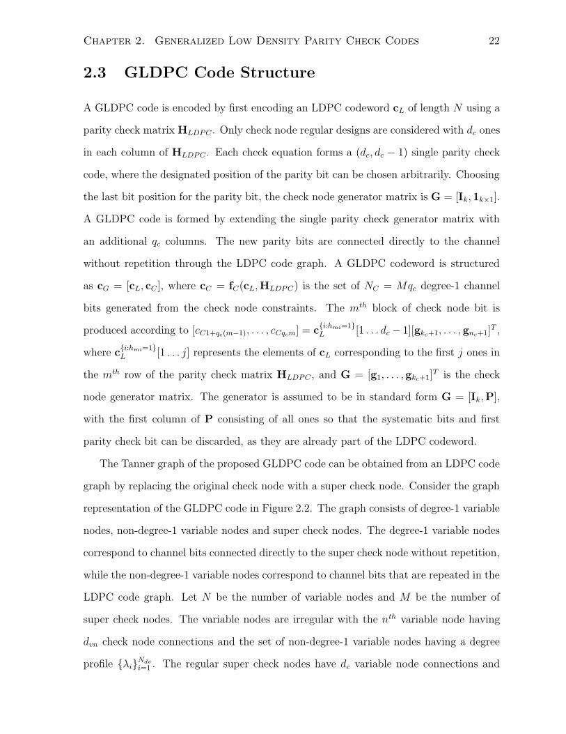
2.2 Graph of irregular LDPC code with generalized check node . . . . . . . . . . . . 23
2.3 EXIT chart of GLDPC code over BICM channel . . . . . . . . . . . . . . . . . . 30
2.4 EXIT chart for super check nodes with dc = 7 and qc = [0 . . . 6] (left) and
irregular repetition codes with dv = [2 . . . 8] (right) . . . . . . . . . . . . . . . . . 33
2.5 BER of GLDPC codes, LDPC codes and LDPC codes with Hadamard constraints
over AWGN channel at rates r = 0.05, 0.1, 0.2, 0.3 for transmission of Nu =
2000 uncoded bits . . . . . . . . . . . . . . . . . . . . . . . . . . . . . . . . . . . 38
2.6 FER of GLDPC codes, LDPC codes and LDPC codes with Hadamard constraints
over AWGN channel at rates r = 0.05, 0.1, 0.2, 0.3 for transmission of Nu =
2000 uncoded bits . . . . . . . . . . . . . . . . . . . . . . . . . . . . . . . . . . . 39
2.7 Rate-loss of GLDPC and LDPC codes as a function of rate for Nc = 250, 4000 41
2.8 Power-loss of GLDPC and LDPC codes as a function of rate for Nc = 250, 4000 42
xii
2.9 Rate-loss for 16-QAM MLCM-MSD transmission using GLDPC (top) and LDPC
(bottom) subcodes and different labelling functions for packet lengths of Nc =
250, 4000 . . . . . . . . . . . . . . . . . . . . . . . . . . . . . . . . . . . . . . . 43
2.10 Rate-loss for 256-QAM MLCM-MSD transmission using GLDPC (top) and LDPC
(bottom) subcodes and different labelling functions for packet lengths of Nc =
250, 4000 . . . . . . . . . . . . . . . . . . . . . . . . . . . . . . . . . . . . . . . 44
2.11 FER of LDPC and GLDPC coded MLCM-MSD systems over AWGN channel
using 16-QAM . . . . . . . . . . . . . . . . . . . . . . . . . . . . . . . . . . . . . 45
2.12 Conditional pdf of messages from the first subchannel using Gray and Anti-
Natural labelling at transmission rates r = 1, 2 . . . . . . . . . . . . . . . . . . 46
2.13 Comparison of GLDPC coded BICM-IDD and MLCM-MSD transmissions at
rates r = 1, 2, 3 . . . . . . . . . . . . . . . . . . . . . . . . . . . . . . . . . . . . 47
3.1 Recursive systematic convolutional code with generator goct = [7 5], with corre-
sponding trellis. Also shown is the projected trellis over m0 = 3 space. . . . . . . 54
3.2 EXIT Curves for rate 1/2, 1/4 convolutional outer codes for code memory
M = 1, . . . , 7 . . . . . . . . . . . . . . . . . . . . . . . . . . . . . . . . . . . . . 59
3.3 EXIT curves for punctured subcode set for code memory M = 1, . . . , 7 . . . . . 64
3.4 Channel EXIT curves for different 16-QAM mapping functions over the AWGN
and 2× 2 MIMO fading channel. . . . . . . . . . . . . . . . . . . . . . . . . . . . 67
3.5 Optimized outer code EXIT curve for different mapping functions over the AWGN
channel at a binary code rate of 1/2 . . . . . . . . . . . . . . . . . . . . . . . . . 69
3.6 FER performance of 16-QAM BICM system over AWGN channel using fixed and
variable sized trellises. . . . . . . . . . . . . . . . . . . . . . . . . . . . . . . . . . 71
3.7 AWGN channel performance of proposed codes for 2000 symbol transmissions. . 72
3.8 AWGN channel performance of proposed codes for 250 symbol transmissions. . . 72
3.9 2 × 2 MIMO channel performance using proposed codes for 1000 symbol trans-
missions. . . . . . . . . . . . . . . . . . . . . . . . . . . . . . . . . . . . . . . . . . 73
xiii
3.10 2 × 2 MIMO channel performance using proposed codes for 125 symbol trans-
missions. . . . . . . . . . . . . . . . . . . . . . . . . . . . . . . . . . . . . . . . . . 74
4.1 Layered Space-Time Transmitter . . . . . . . . . . . . . . . . . . . . . . . . . . . 78
4.2 IDD Layered Receiver . . . . . . . . . . . . . . . . . . . . . . . . . . . . . . . . . 79
4.3 Uncoded BER performance of RDMAP and GMAP detectors for N = 6, M = 6
system using QPSK modulation with NG = 1, 2, 3, 4. . . . . . . . . . . . . . . . 92
4.4 Uncoded BER performance of RDMAP and GMAP detectors for QPSK system
with N = 6, NG = 3 and different M . . . . . . . . . . . . . . . . . . . . . . . . . 93
4.5 Coded BER comparison of RDMAP, GMAP, MMSE, and MAP detectors using
QPSK for N = 6, M = 3 system and N = 6, M = 5 system. Group size NG = 4
for the RDMAP and GMAP detectors. . . . . . . . . . . . . . . . . . . . . . . . . 94
4.6 Coded BER as a function of the number of turbo iterations for RDMAP and
GMAP detectors using QPSK for N = 6, M = 3 system with NG = 4. . . . . . . 96
4.7 Coded BER comparison of RDMAP and GMAP detectors for N = 10, M = 4
QPSK system with NG = 1, 2, 4, 5. . . . . . . . . . . . . . . . . . . . . . . . . . . 97
4.8 Coded BER comparison of MMSE, RDMAP and GMAP detectors for N =
4, M = 2 system using 16-QAM modulation with NG = 2, 4. . . . . . . . . . . . . 98
5.1 Space-Time MLCM Transmitter . . . . . . . . . . . . . . . . . . . . . . . . . . . 103
5.2 CM capacity as a function of the unconstrained capacity for unprecoded and
isotropic unitary precoded systems . . . . . . . . . . . . . . . . . . . . . . . . . . 111
5.3 Subchannel capacities as a function of the CM Capacity for unprecoded system . 113
5.4 Subchannel capacities as a function of the CM Capacity for spatial interleaving
and isotropic unitary precoding . . . . . . . . . . . . . . . . . . . . . . . . . . . . 114
5.5 Subchannel capacities as a function of the unconstrained capacity for random
labelling with and without random isotropic unitary precoding . . . . . . . . . . 116
5.6 FER performance of BICM-IDD and MLCM-MSD systems using QPSK over
2 × 2 quasi-static Rayleigh fading channel for different mapping and precoder
choices . . . . . . . . . . . . . . . . . . . . . . . . . . . . . . . . . . . . . . . . . . 123
xiv
5.7 FER performance of BICM-IDD and MLCM-MSD systems using 16-QAM over
2 × 2 quasi-static Rayleigh fading channel for different mapping, precoder and
detector choices. Target error rate of FER=0.005 . . . . . . . . . . . . . . . . . . 124
5.8 FER performance of BICM-IDD and MLCM-MSD systems using 16-QAM over
2 × 2 quasi-static Rayleigh fading channel for different mapping, precoder and
detector choices. Target error rate of FER=0.1 . . . . . . . . . . . . . . . . . . . 125
5.9 FER performance of BICM-IDD and MLCM-MSD systems using 16-QAM over
2 × 2 quasi-static Rayleigh fading channel for different mapping, precoder and
detector choices and block size Ns = 250. . . . . . . . . . . . . . . . . . . . . . . 126
5.10 FER performance of BICM-IDD and MLCM-MSD systems using QPSK over
4 × 4 quasi-static Rayleigh fading channel for different mapping and precoder
choices . . . . . . . . . . . . . . . . . . . . . . . . . . . . . . . . . . . . . . . . . . 127
5.11 FER performance of BICM-IDD system using 16-QAM over 4 × 4 quasi-static
Rayleigh fading channel for different mapping, and detector choices, and block
size Ns = 1000. . . . . . . . . . . . . . . . . . . . . . . . . . . . . . . . . . . . . . 128
5.12 FER performance of MLCM-MSD system using 16-QAM over 4× 4 quasi-static
Rayleigh fading channel for different mapping, precoder and detector choices,
and block size Ns = 1000. . . . . . . . . . . . . . . . . . . . . . . . . . . . . . . . 129
5.13 FER performance of BICM-IDD and MLCM-MSD system using 16-QAM over
4 × 4 quasi-static Rayleigh fading channel for different mapping, precoder and
detector choices, and block size Ns = 250. . . . . . . . . . . . . . . . . . . . . . . 130
5.14 FER performance of BICM-IDD and MLCM-MSD system using QPSK over 4×2
quasi-static Rayleigh fading channel for different mapping, precoder and detector
choices, and block size Ns = 1000. . . . . . . . . . . . . . . . . . . . . . . . . . . 131
5.15 FER performance of BICM and MLCM system using 16-QAM over 4× 2 quasi-
static Rayleigh fading channel for different mapping, precoder and detector
choices, and block size Ns = 1000. . . . . . . . . . . . . . . . . . . . . . . . . . . 131
xv
5.16 FER performance of BICM-IDD and MLCM-MSD system using 16-QAM over
2× 2 doppler Rayleigh fading channel with ∆fdop = 0.01 for different mapping,
precoder and detector choices, and block size Ns = 1000. . . . . . . . . . . . . . . 133
5.17 FER performance of BICM-IDD and MLCM-MSD system using 16-QAM over
2× 2 doppler Rayleigh fading channel with ∆fdop = 0.01 for different mapping,
precoder and detector choices, and block size Ns = 250. . . . . . . . . . . . . . . 133
5.18 FER performance of BICM-IDD and MLCM-MSD systems using 16-QAM over
2 × 2 Rician channel with unity k-factor for different mapping, precoder and
detector choices, and block size Ns = 1000. . . . . . . . . . . . . . . . . . . . . . 134
5.19 FER performance of BICM-IDD and MLCM-MSD systems using 16-QAM over
2×2 correlated Rayleigh fading channel (α = 0.5) for different mapping, precoder
and detector choices, and block size Ns = 1000. . . . . . . . . . . . . . . . . . . . 135
5.20 FER performance of BICM-IDD and MLCM-MSD systems using 16-QAM over
2× 2 urban microcell environment for different mapping, precoder and detector
choices, and block size Ns = 1000. . . . . . . . . . . . . . . . . . . . . . . . . . . 136
5.21 FER performance of BICM-IDD and MLCM-MSD systems using 16-QAM over
2 × 2 suburban macrocell environment for different mapping, precoder and de-
tector choices, and block size Ns = 1000. . . . . . . . . . . . . . . . . . . . . . . . 137
xvi

Chapter 1
Introduction
1.1 Wireless Communications Background
Wireless personal communications has seen explosive growth in the last twenty years,
finding application in a plethora of consumer devices. In the 1980s, personal wireless
communications was in its infancy, relatively speaking. Passive paging networks and first
generation analog cell phone networks were in place, although cell phones had a high
mobile unit cost and power consumption that limited size, battery life and consumer
accessibility. One also has to mention wireless phone technology that represented the
last leg in the telephony network. In addition, citizens’ band radios continue to be ad
hoc voice networks with low cost walkie talkies handsets that date back to the Second
World War.
At present, a wide array of wireless communications devices play an increasingly
larger role in everyday life. Third generation cell phone systems support an enriched
range of services that include voice, email, internet connectivity, streamed multimedia,
and video conversations. Wireless local area networks first grew with home networking
products that have made their way into businesses and university networks with improved
security and reliability. Wireless local area networks have permeated public places such
1
Chapter 1. Introduction 2
as hotels, cafes, malls and convention facilities. Broadband wireless is encroaching on
the market that provides the last mile of service, traditionally dominated by cable and
digital subscriber line providers. Finally, a wide range of products have been developed
based on wireless personal area networks, such as Bluetooth. These products provide
wireless connectivity to hand held, miniature and peripheral devices.
Next generation wireless systems are converging based on the demand for high-
bandwidth multimedia applications over packet based networks. Transmission through-
put comes at the cost of other system constraints such as transmission power that is
limited by battery life, and spectral bandwidth that is often shared by a number of users.
The capacity of the physical wireless channel is limited by channel fading characteristics.
In a scattered fading environment where multiple reflections of the transmitter signal
are received, random motion leads to periods where the reflected signals interfere de-
structively. Periods of destructive interference or deep fades make it difficult to transmit
reliably with at a high throughput. Multi-antenna communications has emerged as a
means to mitigate fading, because of the large number of wireless links between trans-
mitter and receiver antenna pairs. It has been shown that the channel capacity grows
with the minimum of the number of transmitter and receiver antennas in highly scattered
environments [1, 2]
1.2 Coded Modulation
Most data communication systems involve some kind of error correcting code, and high
throughput applications often require a non-binary modulation format. Many wireless
transmissions can be thus classified as coded modulation systems, involving one or more
binary codes connected to a mapping or modulation block. An early form of coded
modulation is trellis coded modulation, which has been employed for a number of years
in telephone modems [3]. Trellis coded modulation is a multilevel code that maps different
Chapter 1. Introduction 3
S/POuter
Code P
Pre
coder
Mapper
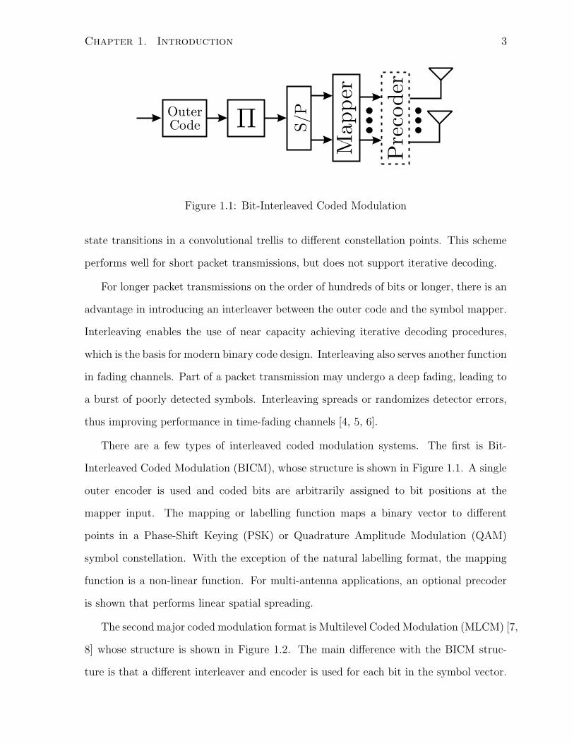
Figure 1.1: Bit-Interleaved Coded Modulation
state transitions in a convolutional trellis to different constellation points. This scheme
performs well for short packet transmissions, but does not support iterative decoding.
For longer packet transmissions on the order of hundreds of bits or longer, there is an
advantage in introducing an interleaver between the outer code and the symbol mapper.
Interleaving enables the use of near capacity achieving iterative decoding procedures,
which is the basis for modern binary code design. Interleaving also serves another function
in fading channels. Part of a packet transmission may undergo a deep fading, leading to
a burst of poorly detected symbols. Interleaving spreads or randomizes detector errors,
thus improving performance in time-fading channels [4, 5, 6].
There are a few types of interleaved coded modulation systems. The first is Bit-
Interleaved Coded Modulation (BICM), whose structure is shown in Figure 1.1. A single
outer encoder is used and coded bits are arbitrarily assigned to bit positions at the
mapper input. The mapping or labelling function maps a binary vector to different
points in a Phase-Shift Keying (PSK) or Quadrature Amplitude Modulation (QAM)
symbol constellation. With the exception of the natural labelling format, the mapping
function is a non-linear function. For multi-antenna applications, an optional precoder
is shown that performs linear spatial spreading.
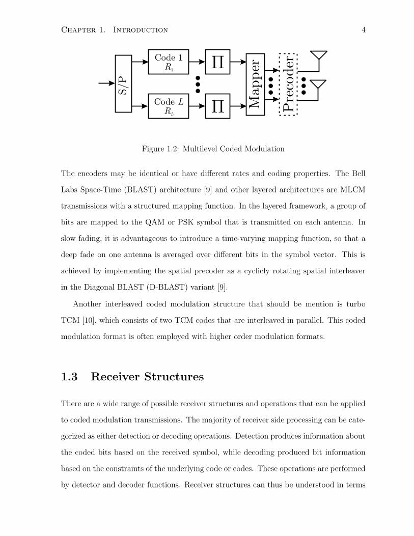
The second major coded modulation format is Multilevel Coded Modulation (MLCM) [7,
8] whose structure is shown in Figure 1.2. The main difference with the BICM struc-
ture is that a different interleaver and encoder is used for each bit in the symbol vector.
Chapter 1. Introduction 4
S/P
Code 1R1
P
Code L
RL
P Pre
coder
Mapper
Figure 1.2: Multilevel Coded Modulation
The encoders may be identical or have different rates and coding properties. The Bell
Labs Space-Time (BLAST) architecture [9] and other layered architectures are MLCM
transmissions with a structured mapping function. In the layered framework, a group of
bits are mapped to the QAM or PSK symbol that is transmitted on each antenna. In
slow fading, it is advantageous to introduce a time-varying mapping function, so that a
deep fade on one antenna is averaged over different bits in the symbol vector. This is
achieved by implementing the spatial precoder as a cyclicly rotating spatial interleaver
in the Diagonal BLAST (D-BLAST) variant [9].
Another interleaved coded modulation structure that should be mention is turbo
TCM [10], which consists of two TCM codes that are interleaved in parallel. This coded
modulation format is often employed with higher order modulation formats.
1.3 Receiver Structures
There are a wide range of possible receiver structures and operations that can be applied
to coded modulation transmissions. The majority of receiver side processing can be cate-
gorized as either detection or decoding operations. Detection produces information about
the coded bits based on the received symbol, while decoding produced bit information
based on the constraints of the underlying code or codes. These operations are performed
by detector and decoder functions. Receiver structures can thus be understood in terms

Chapter 1. Introduction 5
Det. 1P
-1
PDec. 1
Det. 2P
-1
PDec. 2
Det. LP
-1
PDec. L
y1
y2
yM
y
^b1
^b2
^ bL
Figure 1.3: Multistage Decoder
of how the detector and decoder block are connected and interact.
The simplest receiver structure is the one-shot receiver that calls the detector once and
passes coded bit information to the decoder, which then produces uncoded bit decisions.
The one-shot receiver can be applied to either BICM or MLCM transmissions, although it
is in general not capacity achieving for higher order modulation formats. Gray labelling
is typically used with this structure so as to minimized detector message correlation.
More correlated labelling functions require decoder feedback in order to avoid significant
performance loss.
The next receiver structure is the MultiStage Decoder (MSD), shown in Figure 1.3.
The MSD is based on sequential detection and decoding of bits in the symbol vector. At
the lth stage, the lth bit in the symbol vector is detected and decoded, using previously
decoded bit decisions in the detection operation. In order to perform complete decoding
at each stage, each bit in the symbol vector must be encoded independently, thus the MSD
can only be applied to MLCM transmissions. MLCM-MSD systems are near capacity
achieving for many channels with appropriately constructed subcodes. They are less
effective for shorter packet transmissions because of the block length reduction associated
with using independent subcodes.
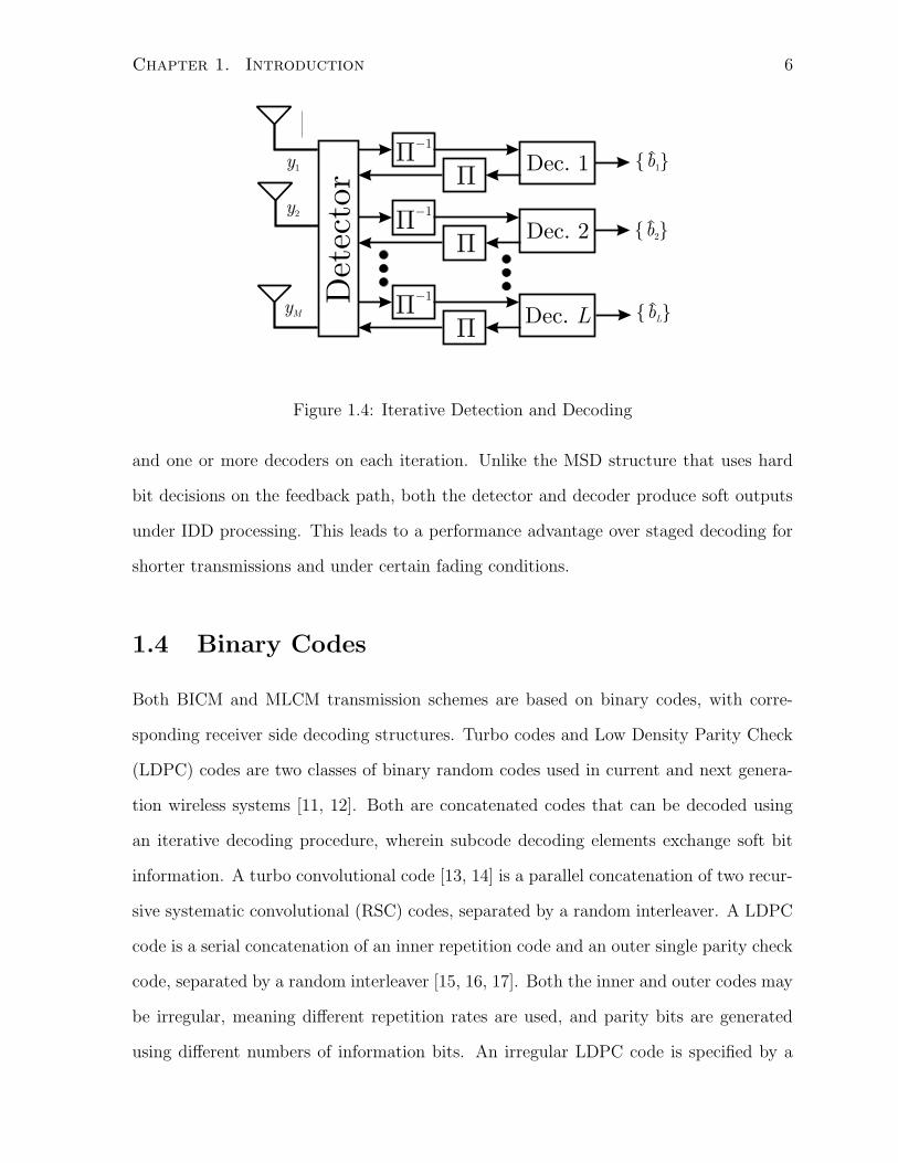
The last receiver structure is the Iterative Detection and Decoding (IDD) structure,
shown in Figure 1.4. The IDD receiver passes soft bit information between the detector
Chapter 1. Introduction 6
y1
y2
yM
^b1
^b2
^ bL
Det
ecto
r
P-1
PDec. 1
P-1
PDec. 2
P-1
PDec. L
Figure 1.4: Iterative Detection and Decoding
and one or more decoders on each iteration. Unlike the MSD structure that uses hard
bit decisions on the feedback path, both the detector and decoder produce soft outputs
under IDD processing. This leads to a performance advantage over staged decoding for
shorter transmissions and under certain fading conditions.
1.4 Binary Codes
Both BICM and MLCM transmission schemes are based on binary codes, with corre-
sponding receiver side decoding structures. Turbo codes and Low Density Parity Check
(LDPC) codes are two classes of binary random codes used in current and next genera-
tion wireless systems [11, 12]. Both are concatenated codes that can be decoded using
an iterative decoding procedure, wherein subcode decoding elements exchange soft bit
information. A turbo convolutional code [13, 14] is a parallel concatenation of two recur-
sive systematic convolutional (RSC) codes, separated by a random interleaver. A LDPC
code is a serial concatenation of an inner repetition code and an outer single parity check
code, separated by a random interleaver [15, 16, 17]. Both the inner and outer codes may
be irregular, meaning different repetition rates are used, and parity bits are generated
using different numbers of information bits. An irregular LDPC code is specified by a

Chapter 1. Introduction 7
code profile, which is the relative fraction of different repetition rates and parity bits
used to generate the code.
For long code construction, irregular LDPC codes can be designed to perform to
within a fraction of a decibel of the channel capacity. Turbo codes have higher error
floor, and incur significant decoding latency for longer code lengths because of the serial
nature of encoding and decoding. For shorter transmissions, message correlation in the
decoding process tends to limit performance. The LDPC code graphs is sparse and more
sensitive to message correlation, where as the convolutional trellis is more structured
and less affected by message correlation. Accordingly, convolutional turbo codes tend to
outperform LDPC codes at shorter block lengths.
The design and analysis of LDPC and convolutional turbo codes is well understood
for binary channels such as the binary Additive White Gaussian Noise (AWGN) chan-
nel [13, 14, 16, 17]. Code design rules can be derived from the analysis of the iterative
decoding process, typically under the assumption that the decoding graph is loop-free.
Under the loop-free assumption, LDPC code performance can be predicted by analyzing
the evolution of the check and repetition node message densities [18]. Within a density
evolution framework, an irregular LDPC code profile can be found through optimiza-
tion, although the process is computational intensive. In order to simplify analysis, the
message densities are often assumed to be Gaussian. With the Gaussian assumption,
the convergence process can be visualized in an Extrinsic Information Transfer (EXIT)
chart, which can be constructed for convolutional turbo codes [19] and LDPC codes [20].
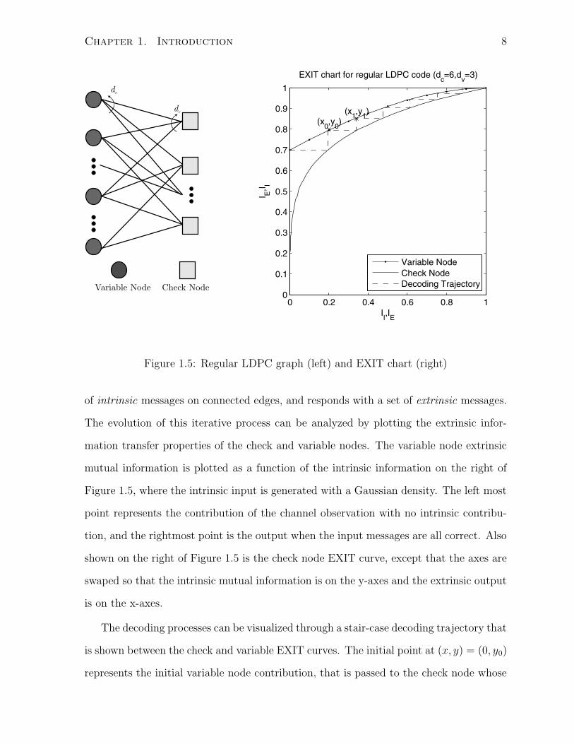
EXIT chart analysis is applied throughout this dissertation and is worth some dis-
cussion. Consider a regular LDPC code with dv parity checks per bit and dc bits per
parity check. The bi-partite graph representing such a code is shown in Figure 1.5 on the
left, where the variable and check nodes correspond to repetition and single parity check
codes. Decoding is accomplished through an iterative exchange of messages between
check and variable node elements. On each iteration, each node element receives a set
Chapter 1. Introduction 8
Variable Node Check Node
dv
dc
Figure 1.5: Regular LDPC graph (left) and EXIT chart (right)
of intrinsic messages on connected edges, and responds with a set of extrinsic messages.
The evolution of this iterative process can be analyzed by plotting the extrinsic infor-
mation transfer properties of the check and variable nodes. The variable node extrinsic
mutual information is plotted as a function of the intrinsic information on the right of
Figure 1.5, where the intrinsic input is generated with a Gaussian density. The left most
point represents the contribution of the channel observation with no intrinsic contribu-
tion, and the rightmost point is the output when the input messages are all correct. Also
shown on the right of Figure 1.5 is the check node EXIT curve, except that the axes are
swaped so that the intrinsic mutual information is on the y-axes and the extrinsic output
is on the x-axes.
The decoding processes can be visualized through a stair-case decoding trajectory that
is shown between the check and variable EXIT curves. The initial point at (x, y) = (0, y0)
represents the initial variable node contribution, that is passed to the check node whose

Chapter 1. Introduction 9
output has extrinsic mutual information x0, represented by the point (x, y) = (x0, y0).
Based on the check node output x0, the variable node outputs y1, followed in turn by the
check node output x1. The decoding process continues to the point where the variable
and check node curves intersect. If this point is at x = y = 1, then the messages are all
correct and successful decoding is predicted. If on the other hand the two curve intersect
a some point before x = y = 1, some messages bits are in error causing a packet decoding
error. One constraining factor in the decoding analysis is the shape of the detector and
decoder curves. The region between the two curves needs to be minimized, as this area
approximately represents the code’s capacity loss [21]. The check and variable node
EXIT curves are generally chosen to approximately match, so that a decoding tunnel is
opened with a small increase in the channel Signal-to-Noise power Ratio (SNR).
For non-binary channels, the code design problem depends on the receiver structure.
When the iterative receiver is applied, EXIT chart analysis can be used to design either
the outer code in a BICM transmission, or a set of identical subcodes in a MLCM
transmission. A non-concatenated outer code may be used, since iterative processing
is applied between the detector and decoder. In fact, using a concatenated outer code
can increase receiver latency, since several decoder sub-iteration are required for each
detector call. Most often a single outer code such as a convolutional code is employed.
In this case, EXIT charts can be used to match the detector and decoder EXIT curves.
The mapping function strongly influences the slope of the detector curve, while code
properties determine the shape of the decoder curve.
The MSD receiver can only be applied to MLCM transmissions. The subcodes in an
MLCM transmission are determined through a decomposition of the channel capacity
into a set of virtual binary channels. The channel capacity C = I(b;y) is the mutual
information between the binary symbol vector b and noisy channel observation y. This
Chapter 1. Introduction 10
capacity can be decomposed as
I(B;y) = I(b1;y) + I(b2;y|b1) + . . . + I(bL;y|b1, . . . ,bL−1) (1.1)
= C1 + C2 + . . . CL (1.2)
where Cl is the capacity of the lth virtual channel. The lth virtual subchannel is formed
using a single information bit bl, assuming lower index bits bi, i < l are known, and
treating higher index bits bi, i > l as a noise contribution. These channels are virtual
since they require knowledge of lower index bits. Knowledge of lower index bits is only
available in a multistage receiver, provided that previous decoded stages are error-free.
Error-free decoding is ensured by encoding each symbol bit at rate slightly lower rate
than the corresponding subchannel capacity. The distribution of subchannel capacities
is largely determined by the mapping scheme used.
1.5 Fading
Fading generally refers to the fluctuation in the envelope of the transmitted signal. The
classification of fading depends on the distances considered. Over a large distance scale,
the gradual attenuation of the receiver signal as a function of physical distance is known
as large-scale fading or path-loss. Over a small distances, rapid fluctuations in the signal
envelope is referred to as small-scale fading. This phenomena stems from the fact that
the received signal contains many reflections of the transmitted signal with different am-
plitudes and phases. Phase differences are far more critical than variations in amplitude,
as the former can give rise to destructive interference which significantly limits channel
capacity. The mitigation of small-scale fading is a central concern in wireless transceiver
design.
Small-scale fading can be further classified based on the symbol interval used. If the
multi-path components have a delay spread that is comparable or longer than the symbol
Chapter 1. Introduction 11
time, then the signal undergo frequency-selective fading that leads to Inter-Symbol In-
terference (ISI). Frequency-selective fading is maybe accommodated with a multi-carrier
modulation such as Orthogonal Frequency Division Multiplexing (OFDM), which uses a
set of orthogonal sub-carriers that each sees a frequency-flat channel. The symbol time
is also key factor when considering time-varying channel characteristics. If the channel
undergos significant changes over a few symbols, then it is classified as a fast-fading chan-
nel, otherwise it is known as a slow-fading channel. In a fast-fading environment where
channel estimation may be difficult, differential modulation is often used as it enables de-
tection without explicit channel knowledge. A limiting case of slow-fading is quasi-static
fading, wherein the channel remains constant for the duration of a packet transmission.
Channel fading characteristics significantly affect link capacity and reliability. High
throughput reliable communications is particularly problematic in a frequency-flat quasi-
static fading channel. The quasi-static fading condition means that if the channel is bad,
it is bad for the whole packet, and that packet will likely be decoded erroneously. A time-
varying channel will average good and bad portions of the channel, and it is unlikely the
channel will remain bad for an entire packet. A frequency-flat channel is one where the
entire transmission bandwidth experiences the same fading phenomenon, be it good or
bad. In frequency selective fading, different parts of the transmission bandwidth undergo
different fading phenomena, and it is improbable that the entire spectrum will be in a
deep fade.
For multi-antenna communications, the spatial fading properties of the wireless chan-
nel become more significant. The simplest spatial fading channel is the Rayleigh channel,
which assumes an infinite number of isotropically distributed scatters with no line-of-
sight component. The addition of a line-of-sight component leads to Rician fading with
a slight increases in channel capacity. Antenna correlation due to insufficient antenna
spacing is often modelled with a correlated Rayleigh channel model. A number of more
realistic channel models have been developed to model indoor and outdoor wireless chan-

Chapter 1. Introduction 12
nels [22, 23, 24, 25, 26, 27]. These models account for antenna geometries and polariza-
tion, as well as different environmental scenarios such as urban versus rural conditions.
Particular fading scenarios such as the urban canyon [26, 27] and keyhole fading [24, 28]
around building openings have also been modelled.
1.6 Multi-Antenna Communications
Multi-antenna communications can improve both the reliability and data throughput of
a wireless link. Transmission reliability is improved through spatial diversity, wherein
redundant copies of the transmitted signal are sent on different transmitter antennas.
Transmission throughput can be increased through spatial multiplexing, which sends
independent data on each transmitter antenna. In the high SNR region, transmission
capacity grows with the minimum of the number transmitter and receiver antennas in a
scattered environment [1, 2]. There is a tradeoff between diversity and multiplexing, such
that increased capacity comes at the cost of reduced diversity. A broad range of multi-
antenna coding strategies have been developed that exploit diversity and multiplexing
gains to different degrees. These strategies can be classified based on the number of
symbols spanned by the underlying code or coded modulation scheme.
Transmissions of a few symbols are best coded with space-time block codes. These
codes are generally based on transmitting multiple copies of symbols on different trans-
mitter antennas with appropriate scaling. The code structure and coefficients are often
determined using rank and determinant criteria derived from the eigenvalue distribu-
tion of the combined code/channel correlations matrix [29]. The well known Alamouti
code [30] is a rate-one orthogonal space-time block code for two transmitter antennas.
This design has been generalized to larger systems in [31], however, there is a rate limita-
tion with orthogonal designs. Higher rates are possible with quasi-orthogonal space-time
block codes [32, 33], which relax the constraint of linear decoding complexity for ad-

Chapter 1. Introduction 13
ditional rate. Linear dispersion codes are a class of space-time block codes whose code
coefficients are found through numerical optimization. Optimization techniques based on
both mutual information and the determinant and rank criteria were initially proposed
in [34], but better performance is possible by direct minimization of the block error rate
through stochastic gradient search methods [35].
For transmissions longer than a few symbols, Maximum Likelihood (ML) decoding
performance is not possible using space-time block codes alone because of the computa-
tional infeasibility. Space-time trellis coded modulation systems have been proposed [29]
whose state mapping is determined through the rank and determinant criteria. For packet
lengths on the order of hundreds of symbols, trellis coded modulation is outperformed
by time-interleaving schemes such as BICM or MLCM.
BICM and MLCM architectures can be extended to space-time applications thorough
the choice of the symbol mapper and precoder. The precoder is the linear component
of the space-time coded modulation and the symbol mapper the non-linear component.
Spatial precoders have been designed for BICM systems under different fading condi-
tions [36, 37, 38, 39, 40, 41, 42]. In the MLCM framework, the D-BLAST variant of the
layered architecture implements the spatial precoder as a spatial interleaver. This leads
to a performance improvement under slow and quasi-static fading conditions. Precoders
have also been designed correlated for fading channels [43, 44]
Multi-dimensional mapping is a particularly useful coding strategy under slow fading
conditions. The most promising fade resistant mapping strategy is multi-dimensional
random labelling [45, 46], although other coding and mapping strategies have been pro-
posed [47]. Multi-dimensional random labelling generally uses a pseudo-random mapping
function that changes between symbols and is known at the receiver. Random map-
ping leads to highly correlated detector symbol messages, whose statistical properties
are less sensitive to the effects of fading. In a MLCM-MSD framework, near capac-
ity achieving performance is possible using random labelling under quasi-static fading

Chapter 1. Introduction 14
conditions [45, 46].
Multi-dimensional random labelling posses a few design challenges. Since random
labelling requires optimal detection, it may be computationally infeasible for large sys-
tems. In MLCM-MSD transmissions, random labelling leads to a large subchannel ca-
pacity spread that requires subcodes to be designed over a wide range of rates. The
LDPC codes used in [45, 46] incur a significant capacity loss for low rate subcodes.
In BICM-IDD transmissions, random labelling leads to steeply sloped channel EXIT
curves. This is problematic for many existing code design procedures. To our knowledge,
multi-dimensional random labelling has not been used in BICM systems to mitigate slow
fading.
1.7 Scope and Overview
There are range of wireless communications systems that can benefit from multi-antenna
solutions. Many of these systems involve multiple users sharing the communications chan-
nel, and others involve multi-carrier modulation formats, such as OFDM, that mitigate
the effects of frequency selective fading. As the focus of this work is on the multi-antenna
aspects of the system, the remaining design factors will be kept as simple as possible.
To this end, the scope of this dissertation is limited to single-carrier single-user trans-
missions of an independent binary data source. Extensions to multimedia applications,
multi-carrier OFDM, and multiuser systems are discussed as future work in Chapter 6.
In addition, we only consider coded modulation designs with transmissions lengths in
the range of hundreds-to-thousands of symbols. We also focus on high-rate designs that
exploit the multiplexing gain of multi-antenna wireless channels.
The next major design considerations are the channel fading characteristics and how
the channel is know at the transmitter and receiver. We consider frequency-flat fading
channels, and focus on the slow fading scenario where channel coherence time is signif-
Chapter 1. Introduction 15
icantly larger than the symbol time. Under slow-fading conditions, there is negligible
ISI due to Doppler in the pulse shaping filter, and channel estimation is generally not
a challenging problem. Channel estimation is avoided altogether in this dissertation by
assuming perfect channel state information (CSI) at the receiver. It is further assumed
that CSI is not available to the transmitter.
Different transmitter and receiver configurations are considered. Precoder and map-
per designs are proposed for BICM and MLCM transmissions based on channel fading
characteristics and receiver complexity constraints. Two suboptimal detectors are pro-
posed based on a group detection strategy. Within a BICM-IDD framework, a class of
irregular convolutional codes are proposed, which can be designed to suit different chan-
nel conditions. For MLCM-MSD systems, a class of generalized LDPC codes is proposed
with performance gains over fading and non-fading channels.
Chapter 2 examines the use of LDPC codes in coded modulation systems. For finite
length MLCM-MSD transmissions, set partitioning labelling minimizes capacity loss pro-
vided that efficient binary codes can be constructed over a wide rate range. Conventional
LDPC codes perform well for moderate-to-high rate construction, but not in the low rate
region. A class of generalized LDPC codes is proposed with improved low rate perfor-
mance. This is achieved through a generalized check node that connects additional check
node parity bits to the channel without repetition. The proposed generalized LDPC
codes can also be designed for BICM-IDD systems.
Chapter 3 develops an irregular convolutional code construction procedure within a
BICM-IDD system. A convolutional code can be made irregular using generator polyno-
mials of different memory, and a set of puncture patterns that produce different subcode
rates. The generator/puncture pattern combination makes a subcode, and the weighted
sum of subcodes forms the overall code. An irregular code profile is determined through
EXIT chart analysis, and different concatenation strategies are proposed to connect vary-
ing size trellises. The proposed codes outperform turbo codes and MLCM-MSD designs

Chapter 1. Introduction 16
over multi-antenna channels.
Chapter 4 develops two detectors based on a group detection strategy that can op-
erate within a IDD receiver. These detectors are useful in systems having a large con-
stellation and number of transmitter antennas, such that the optimal detector becomes
computationally infeasible. A suboptimal decision is made using a subset of the symbol
vector, treating the remaining signal contribution as noise that is suppressed through
filtering. The proposed detectors have a significant performance improvement over linear
processing detectors in spatially multiplexed systems having fewer receiver antennas than
transmitter antennas.
Chapter 5 tackles the problem of multi-antenna precoder and mapper design under
slow fading. The BICM and MLCM coding strategies developed in Chapter 2 and Chap-
ter 3 are extended to the slow fading conditions, and the detection strategies developed
in Chapter 4 are applied where appropriate. Isotropic unitary random precoding is pre-
sented as an alternative to the spatial interleaving strategy used in layered multiplexing
schemes. Unitary precoding does not affect receiver complexity and allows the use of a
linear detector. Random multidimensional mapping is discussed as an effective non-linear
spatial coding technique that requires a high complexity detector. Under optimal detec-
tion, the IDD receiver is shown to have a fundamental performance advantage over the
MSD receiver in quasi-static fading, regardless of packet length. For large constellations,
a group random mapping strategy is proposed for MLCM-MSD systems where optimal
detection is not feasible.

Chapter 2
Generalized Low Density Parity
Check Codes
Low density parity check codes are widely used in coded modulation systems in both bit-
interleaved and multilevel coded modulation structures. In MLCM systems, set partition
labelling has a rate advantage over other formats, but generates a wide range of sub code
rates that may be difficult to implement. Conventional LDPC code construction incurs
a significant capacity loss for low rate subcodes. A class of generalized LDPC codes is
proposed in this chapter that improves conventional LDPC code performance in the low
rate region. These codes are designed for MSD and IDD decoding.
2.1 Introduction
The interaction between the code and mapping function plays a large role in the design
of coded modulation systems. For LDPC binary code, Gray mapping has traditionally
been used in both MLCM and BICM configurations. Gray mapping minimizes capacity
loss when the one-shot receiver is applied [5, 48, 49, 50]. Other labelling schemes have
been proposed for BICM-IDD systems [6, 51, 52, 53], however Gray mapping is still a
good choice with LDPC outer codes [20]. In the MLCM-MSD structure, set partitioning
17
Chapter 2. Generalized Low Density Parity Check Codes 18
labelling was originally proposed in [7] and was later shown to have better performance
than other labelling formats [8] for finite length transmissions. Set partitioning has a
capacity advantage over over schemes under MSD decoder, but generally requires efficient
subcodes to be designed over a wide range of rates.
Low Density Parity Check (LDPC) codes [15] have been the subject of great interest
since their rediscovery in [16, 17] because of their Shannon capacity approaching per-
formance with a simple belief propagation (BP) decoder. A conventional LDPC code is
based on a sparse parity check matrix whose rows represent single parity check codes and
whose columns represent repetition codes. Several generalized LDPC codes have been
proposed [54, 55, 56, 57, 58, 58, 59, 60] that replace the single parity check codes with
other block codes.
Existing LDPC and Generalized LDPC (GLDPC) designs, with the exception of [60],
have limitations in the low rate region. Low code rates lead to variable node performance
that is relatively insensitive to changes in the SNR, thus incurring a significant SNR
penalty to open a decoding tunnel. In addition, low rate LDPC codes have parity check
matrices that are almost square, for which it is difficult to find high girth graphs at
moderate code lengths because of the large relative number of check equations. The
solution in [60] is to link the check node performance to the channel SNR by connecting
additional parity bits directly to the channel. The Hadamard check node used in [60] has
limited design options, since it is only suited for the very low rate range R ≤ 0.05.
This chapter develops a set of irregular LDPC codes with generalized check nodes
having improved low rate r < 1/3 performance. These codes can improve MLCM-MSD
performance over a wide range of design rates when set partitioning labelling is used. Set
partitioning labelling generates a large spread of subcode rates, thereby benefitting from
improved low rate construction. It will be shown that mapping schemes generating low
and very high rate subcodes have a rate advantage over Gray mapping, which produces
concentrated subcode rates.
Chapter 2. Generalized Low Density Parity Check Codes 19
An LDPC code is generalized by extending the single parity codes with additional
parity bits that are connected directly to the channel without repetition. For binary
channels or virtual binary channels in a staged decoder, irregular code profiles can be
found through optimization over a conventional 2-dimensional EXIT chart. For BICM-
IDD designs, the variable and check node EXIT curves are mutually dependent, requiring
several 2-dimensional EXIT chart optimizations within a fixed point iteration framework.
Only check node regular designs are considered. The check node generator matrix is found
through area maximization, also within an EXIT chart framework.
2.2 Multilevel Coded Modulation Design
This section examines MLCM-MSD design for finite length construction. Consider a
modulated symbol s that has a symbol alphabet of size 2L, that is formed according to
s = m(b), where b ∈ BL. The symbol is passed through an AWGN channel according to
y = s + n (2.1)
where n is a complex AWGN noise source with variance σ2n. The set subcode rates is
determined through a decomposition of the constrained modulation (CM) capacity, which
is given by
CCM = I(s; y) = s− Es,y
(
log2
∑
s′∈S p(y|s)p(y|s)
)
(2.2)
= L− Es,y
(
log2
∑
s′∈S exp(‖y − s‖2/(2σ2n))
exp(‖y − s‖2/(2σ2n))
)
(2.3)
where S is the set of possible transmitted symbols, and equiprobable transmitted symbols
and perfect receiver CSI is assumed. The CM capacity can be decomposed into L parallel
subchannels using the chain rule of mutual information as:
I(b; y) = I(b1;y) + I(b2; y|b1) + . . . + I(bL; y|b1, . . . ,bL−1) (2.4)

Chapter 2. Generalized Low Density Parity Check Codes 20
The capacity of each subchannel is Cl = I(bl; y|b1, . . . ,bl−1), provided that lower level
subchannel bits have been decoded correctly. The decomposition in (2.4) implies that
if an MLCM encoding is used with code rates that are matched to the subchannel ca-
pacities rl = Cl, a multistage decoding strategy can be applied with capacity achieving
performance [7, 8] for ideal subcodes. For practical codes, a subcode rate less than the
corresponding capacity must be used to ensure the desired level of FER performance.
A detection error is declared if there is an error in any level, and detection errors ap-
pear relatively independently across subchannels under correct decision feedback. Let
fNcFER(r, C) be the FER of a GLDPC code of length Nc and rate r transmitted across a
binary AWGN channel of capacity C. The optimal set of rates is found by the condition
fNcFER(ri, Ci) = fNc
FER(rj, Cj) ∀ i, j (2.5)
whose optimality is proven in [8, 61].
The total capacity loss∑
l (Cl − rl) is affected by the mapping function that de-
termines the set of subchannel rates, and the FER function fNcFER(r, C). The effect of
mapping on capacity loss was characterized in [8] using random error exponents, and set
partition was found to outperform other labelling schemes. The analysis in [8] does not,
however, give much insight into how capacity loss is affected by the properties of the map-
ping function. Consider the relationship between rate-loss ∆r, which is the rate penalty
paid to sustain a desired level of performance, and power-loss ∆P , which is the addition
transmission power required to sustain that desired level of performance. The entities are
approximately related by derivative approximation ∆P ≈ δPδr
∆r or ∆r ≈ ∆P/ δPδr
, where
δPδr
is the derivative of the power threshold function P (r), which is the minimum SNR
required to support at transmission rate r. The threshold function and its derivative are
shown in Figure 2.1. One can see that the derivative function is lowest in the region
r = [0.4, 0.8] and increases sharply in the low rate region r < 0.25 and the very high rate
region r > 0.9. In the low and very high rate regions, a small subchannel rate-loss leads
to a large increase in the effective SNR of the corresponding virtual channel based on

Chapter 2. Generalized Low Density Parity Check Codes 21
0 0.1 0.2 0.3 0.4 0.5 0.6 0.7 0.8 0.9 1−20
0
20
40
60
80
100
rate
SN
R(d
B)
P(r)dP/dr
Figure 2.1: Plot of the inverse MI function (top) and its derivative (bottom) as a function
of rate for the binary AWGN channel
the derivative approximation. In other words, the power penalty incurred to sustain a
certain level of FER performance translates into a smaller capacity loss in the low and
very high rate regions. It is then advantageous to use mapping functions that generates
subchannel capacities in these regions.
Labelling functions and detection orders that lead to a large spread of subchannel
capacities have a smaller rate-loss than those yielding concentrated capacities. The set
partitioning strategy in [7, 8] maximizes the minimum intra-set distance leading to a
large spread of subcode rates. For an QAM modulation, set partitioning reduces to
natural labelling with a least significant bit first detection order. For the AWGN channel
considered in this chapter, a single code can be mapped to the same bit positions in the
in-phase and quadrature-phase components, thereby doubling the code block length. For
fading channels that are considered in later chapters, the in-phase and quadrature-phase
signal components may experience different degrees of fading, and it is useful to map
separate codes to each signal component.
Chapter 2. Generalized Low Density Parity Check Codes 22
2.3 GLDPC Code Structure
A GLDPC code is encoded by first encoding an LDPC codeword cL of length N using a
parity check matrix HLDPC . Only check node regular designs are considered with dc ones
in each column of HLDPC . Each check equation forms a (dc, dc − 1) single parity check
code, where the designated position of the parity bit can be chosen arbitrarily. Choosing
the last bit position for the parity bit, the check node generator matrix is G = [Ik,1k×1].
A GLDPC code is formed by extending the single parity check generator matrix with
an additional qc columns. The new parity bits are connected directly to the channel
without repetition through the LDPC code graph. A GLDPC codeword is structured
as cG = [cL, cC ], where cC = fC(cL,HLDPC) is the set of NC = Mqc degree-1 channel
bits generated from the check node constraints. The mth block of check node bit is
produced according to [cC1+qc(m−1), . . . , cCqcm] = ci:hmi=1L [1 . . . dc− 1][gkc+1, . . . ,gnc+1]
T ,
where ci:hmi=1L [1 . . . j] represents the elements of cL corresponding to the first j ones in
the mth row of the parity check matrix HLDPC , and G = [g1, . . . ,gkc+1]T is the check
node generator matrix. The generator is assumed to be in standard form G = [Ik,P],
with the first column of P consisting of all ones so that the systematic bits and first
parity check bit can be discarded, as they are already part of the LDPC codeword.
The Tanner graph of the proposed GLDPC code can be obtained from an LDPC code
graph by replacing the original check node with a super check node. Consider the graph
representation of the GLDPC code in Figure 2.2. The graph consists of degree-1 variable
nodes, non-degree-1 variable nodes and super check nodes. The degree-1 variable nodes
correspond to channel bits connected directly to the super check node without repetition,
while the non-degree-1 variable nodes correspond to channel bits that are repeated in the
LDPC code graph. Let N be the number of variable nodes and M be the number of
super check nodes. The variable nodes are irregular with the nth variable node having
dvn check node connections and the set of non-degree-1 variable nodes having a degree
profile λiNdvi=1 . The regular super check nodes have dc variable node connections and
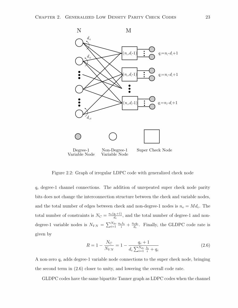
Chapter 2. Generalized Low Density Parity Check Codes 23
q dc c c= - +1n
q dc c c= - +1n
q dc c c= - +1n
Degree-1Variable Node
Non-Degree-1Variable Node
Super Check Node
dv2
(nc, -1)dc
(nc, -1)dc
(nc, -1)dc
dv1
dvN
N M
Figure 2.2: Graph of irregular LDPC code with generalized check node
qc degree-1 channel connections. The addition of unrepeated super check node parity
bits does not change the interconnection structure between the check and variable nodes,
and the total number of edges between check and non-degree-1 nodes is ne = Mdc. The
total number of constraints is NC = ne(qc+1)dc
, and the total number of degree-1 and non-
degree-1 variable nodes is NV N =∑Ndv
i=1neλi
i+ neqc
dc. Finally, the GLDPC code rate is
given by
R = 1− NC
NV N
= 1− qc + 1
dc
∑Ndv
i=1λi
i+ qc
(2.6)
A non-zero qc adds degree-1 variable node connections to the super check node, bringing
the second term in (2.6) closer to unity, and lowering the overall code rate.
GLDPC codes have the same bipartite Tanner graph as LDPC codes when the channel
Chapter 2. Generalized Low Density Parity Check Codes 24
nodes are omitted. It follows that GLDPC codes can be decoded using a BP decoder
with different check node update rules to account for the addition channel connections.
The GLDPC graph in Figure 2.2 has three kinds of connections: variable-to-check node,
variable-to-channel node, and check-to-channel node. Let Uv↔c, Uch↔v and Uch↔c denote
the set of edges between variable and check nodes, channel and variable nodes, and
channel and check nodes, respectively. These three types of bidirectional edges can be
further divided into six types of unidirectional edges denoted, Uv→c, Uc→v, Uch→v, Uv→ch,
Uch→c, and Uc→ch. Associated with each type of edge is a message type and an update
rule for that message type. For the type of v → c edges, let vn be the set of nvn extrinsic
messages coming from variable node n going to check nodes, and let vm be the set of nc
variable node extrinsic messages going to check node m. Since there is only one type of
edge from variable to check nodes, we have vn = vm. For the c → v edge type, let
um, un be the set of extrinsic messages coming from check node m and going to variable
node n. For the Uch↔v edge types, let xn, wn be the extrinsic message coming from and
going to the nth variable node. Similarly, for the Uch↔c edge types, let zm, ym be extrinsic
message vectors of size qc coming from and going to the mth check node.
The update rule for the channel nodes depends on the coded modulation structure.
Based on a channel observation y, an extrinsic output is produced for the lth bit in the
binary symbol vector b according to
λE[bl] = log
∑
b:bl=1 exp(
−‖y−m(b)‖2
σ2n
)
+∑
m log bmeλI [bm]+bm
1+eλI [bm]
∑
b:bl=0 exp(
−‖y−m(b)‖2
σ2n
)
+∑
m log bmeλI [bm]+bm
1+eλI [bm]
− λI [bl] (2.7)
where λI[bl] is the intrinsic input for bit bl. In an MLCM-MSD scheme, each bit is mapped
to a separate code. During the decoding of the lth stage, a constant message is sent
from corresponding channel nodes that is based on channel observations and previously
decoded bits. In the case of the IDD receiver, the channel message is updated every
iteration or at some larger period. In addition, the channel nodes have L connections
instead of the single channel node connections shown in Figure 2.2. These channel node
Chapter 2. Generalized Low Density Parity Check Codes 25
connections are randomly assigned to variable and check nodes. For either the MSD or
IDD receiver structure, the channel updates wn, ym are based on (2.7). Following
the message-passing algorithm in [18], the lth to (l + 1)th stage update equations for the
four remaining message types are given as follows:
vln =
dvn∑
i=1
ulni + wn − ul
n
xln =
dvn∑
i=1
ulni
ul+1mi =
∑
b∈Bkvn ,bi=1 exp(−12bG[vl
m, ylm])
∑
b∈Bkvn ,bi=1 exp(−12bG[vl
m, ylm])− vl
mi
zl+1mi =
∑
b∈Bkvn ,bi=1 exp(−12bG[vl
m, ylm])
∑
b∈Bkvn ,bi=1 exp(−12bG[vl
m, ylm])− yl
mi (2.8)
with v0n = 0, x0
n = 0 ∀ n.
2.4 GLDPC Code Design and Analysis through EXIT
Charts
There are six message densities whose evolution under iterative message passing needs
to be analyzed. Let Ia→b be the average mutual information (MI) conveyed by messages
coming from node type a going to node type b, which is referred to as an extrinsic MI
IEa→b in the update of a and an intrinsic MI IE
a→b in the update of b. The MI for the
six message densities are denoted, Ich→v, Ich→c, Iv→c, Iv→ch, Ic→v, Ic→ch. The evolution of
these message densities can be analyzed using a 2-dimensional EXIT chart [19, 20] in a
fixed point iteration optimization involving the MI functions of all the densities. These
MI functions can be derived by expressing the node update equations in terms of mutual
information. For the channel nodes, it can be observed that the extrinsic MI is the
same for channel-to-variable and channel-to-check node messages, provided that channel
degree-1 bits and non-degree-1 bits are randomly distributed in the symbol vectors. The
Chapter 2. Generalized Low Density Parity Check Codes 26
extrinsic channel MI can be expressed as
IEch→v = IE
ch→c = fch(IIch) (2.9)
where IIch = (1−αD1)I
Iv→ch+αD1I
Ic→ch is the average detector intrinsic MI, and αD1 is the
fraction for degree-1 bits in the GLDPC codeword. For the binary AWGN channel, the
channel message MI can be found in terms of the noise variance as fch(IIch) = J(4/σ2
n) [19],
where
J(σ2Z) = 1−
∫
exp(−(x− σ2Z/2)2/2σ2
Z)√
2πσ2Z
log2[1− e−x]dx (2.10)
IN coded modulation systems, fch(IIch) is determined through Monte Carlo simulations.
For the variable nodes, the MI transfer functions can be derived from the first two update
equations in (2.8) as
IEv→c = fv→c(I
Ic→v, I
Ich→v, λj) =
∑
j
λjJ((j − 1)J−1(IIc→v) + J−1(II
ch→v))
IEv→ch = fv→ch(I
Ic→v, λj) =
∑
j
λjJ(jJ−1(IIc→v)) (2.11)
It will also be useful to represent the inverse functions MI function as I Ic→v = f−1
v→c(IEv→c, I
Ich→v, λj).
The check node MI transfer functions are expressed as
IEc→v = fc→v(I
Iv→c, I
Ich→c)
IEc→ch = fc→ch(I
Iv→c, I
Ich→c) (2.12)
Even though the analysis of the proposed GLDPC codes involves more message types
than for LDPC codes, the optimization of the variable node degree profile remains the
same when the remaining MI functions are fixed. Following the LDPC code EXIT chart
analysis in [20], the variable degree is chosen to maximize the code rate constrained by
the condition that the variable-to-check MI function is greater than the inverse check-to-
variable MI function. This condition is graphically represented by plotting the variable-
to-check MI function on the X − Y axis, plotting the check-to-variable MI function on
the Y − X axis, and ensuring a gap or decoding tunnel exits between the two curves.
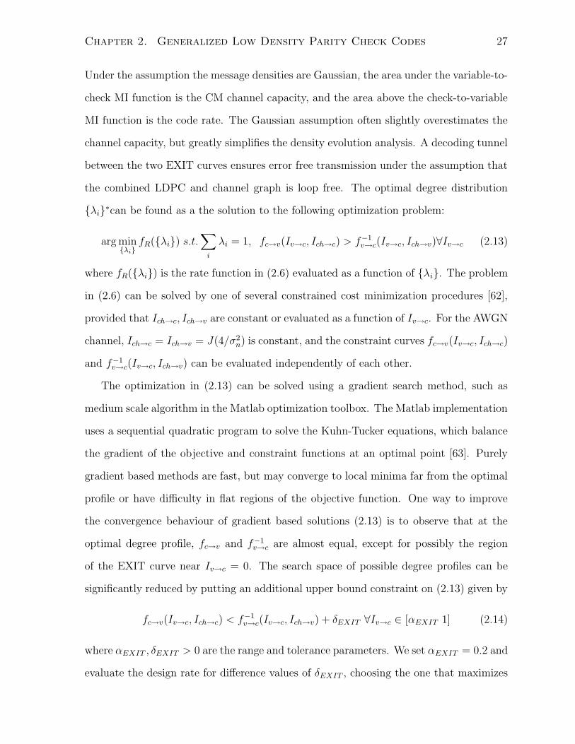
Chapter 2. Generalized Low Density Parity Check Codes 27
Under the assumption the message densities are Gaussian, the area under the variable-to-
check MI function is the CM channel capacity, and the area above the check-to-variable
MI function is the code rate. The Gaussian assumption often slightly overestimates the
channel capacity, but greatly simplifies the density evolution analysis. A decoding tunnel
between the two EXIT curves ensures error free transmission under the assumption that
the combined LDPC and channel graph is loop free. The optimal degree distribution
λi∗can be found as a the solution to the following optimization problem:
arg minλi
fR(λi) s.t.∑
i
λi = 1, fc→v(Iv→c, Ich→c) > f−1v→c(Iv→c, Ich→v)∀Iv→c (2.13)
where fR(λi) is the rate function in (2.6) evaluated as a function of λi. The problem
in (2.6) can be solved by one of several constrained cost minimization procedures [62],
provided that Ich→c, Ich→v are constant or evaluated as a function of Iv→c. For the AWGN
channel, Ich→c = Ich→v = J(4/σ2n) is constant, and the constraint curves fc→v(Iv→c, Ich→c)
and f−1v→c(Iv→c, Ich→v) can be evaluated independently of each other.
The optimization in (2.13) can be solved using a gradient search method, such as
medium scale algorithm in the Matlab optimization toolbox. The Matlab implementation
uses a sequential quadratic program to solve the Kuhn-Tucker equations, which balance
the gradient of the objective and constraint functions at an optimal point [63]. Purely
gradient based methods are fast, but may converge to local minima far from the optimal
profile or have difficulty in flat regions of the objective function. One way to improve
the convergence behaviour of gradient based solutions (2.13) is to observe that at the
optimal degree profile, fc→v and f−1v→c are almost equal, except for possibly the region
of the EXIT curve near Iv→c = 0. The search space of possible degree profiles can be
significantly reduced by putting an additional upper bound constraint on (2.13) given by
fc→v(Iv→c, Ich→c) < f−1v→c(Iv→c, Ich→v) + δEXIT ∀Iv→c ∈ [αEXIT 1] (2.14)
where αEXIT , δEXIT > 0 are the range and tolerance parameters. We set αEXIT = 0.2 and
evaluate the design rate for difference values of δEXIT , choosing the one that maximizes
Chapter 2. Generalized Low Density Parity Check Codes 28
the design rate while keeping the constraints below a certain threshold.
In BICM-IDD systems, the two sides of the second constraint in (2.13) are coupled by
the channel node MI, and the variable degree profile must be jointly analyzed with the
remaining MI functions. Let y = Iv→c be the independent variable typically plotting on
the y-axis of the EXIT chart and let the solution to (2.13) be represented in functional
form as,
λ∗i = fopt(Iv→c, Ic→v, Ich→v) (2.15)
The optimal degree profile can be found from (2.15), provided that Ic→v(y) and Ich→v(y)
can be expressed in terms of y. The entities Ic→v(y) and Ich→v(y) are, however, dependent
on the degree profile through equations (2.11) and (2.9). The MI update equations (2.9),
(2.11) and (2.12), and the degree profile optimization function can be iteratively applied
with the objective of finding a steady-state relationship between the functions Ic→v(y),
Ic→v(y), Ich→v(y), Ich→c(y) and Iv→ch(y) after some number of iterations. The update
equations for the MI functions for the kth iteration, k ≥ 1 are given by,
λ∗jk+1(y) ← fopt(y, Ik
c→v(y), Ikch→v(y))
Ik+1c→v(y) ← f−1
v→c(y, Ikch→v(y), λjk)
Ik+1c→ch(y) ← fc→ch(y, Ik
ch→c(y))
Ikv→ch(y) ← fv→ch(I
kc→v(y), λjk)
Ikch→v(y) = Ik
ch→c(y) ← fch((1− α)Ikv→ch(y) + αIk
c→ch(y)) (2.16)
For the first iteration, the second and fifth update equations in (2.16) are dependent on
the degree profile, which is not available at startup. The effectiveness of the fixed point
update equations is dependent on the initial choices for the MI functions. In order to find
a good initial estimate for the MI functions, we run the MI function update equations
in (2.16) without updating λ∗jk(y) for a few iterations, replacing the second and fifth
Chapter 2. Generalized Low Density Parity Check Codes 29
update equation in (2.16) with
Ik+1c→v(y) ← fc→v(y, Ik
ch→v(y), λjk)
Ikv→ch(y) ← Ik
c→v(y) (2.17)
For the first equation in (2.17), we have used the fact that when a good code profile is
found, fc→v = f−1v→c because of the curve matching property, and in the second equations
we have omitted the function fv→ch. Although in general, fv→ch(y) 6= y, channels that
are well suited to LDPC codes have relatively flat EXIT curves, and the channel MI
function is only slightly affected by a change in the fv→ch(y) function.
The operation of the MI function update equations in (2.16) can be visualized through
an EXIT chart example. Consider a GLDPC coded BICM transmission over an AWGN
channel using 16-QAM modulation, Gray labelling, and a GLDPC code rate of R = 0.25,
with check node parity check matrix
P =
1 0 1 1 0 0
0 1 1 0 1 0
1 0 0 0 1 1
0 1 1 0 0 1
1 1 0 1 0 1
1 1 1 1 1 1
, (2.18)
and variable degree profile λ(x) = 0.156x2 + .738x3 + 0.0634x4 + 0.0146x9 + 0.0146x10 +
0.129x11 found using (2.13) that leads to threshold SNR of 0.48dB, which is the minimum
SNR for which the EXIT constraints are satisfied at the given code rate. The channel ex-
trinsic message MI function Ich→v(x) and the variable-to-check node MI function Iv→c(x)
are plotted in Figure 2.3 on the y-axis against x = Ic→v on the x-axis. Also shown in Fig-
ure 2.3, is the channel extrinsic message MI Ich→c(y) and the variable-to-check node MI
function Iv→c(y) on the x-axis against y = Ic→v on the y-axis. The channel MI functions
seen by the variable and check nodes have the same start and end points, with the one
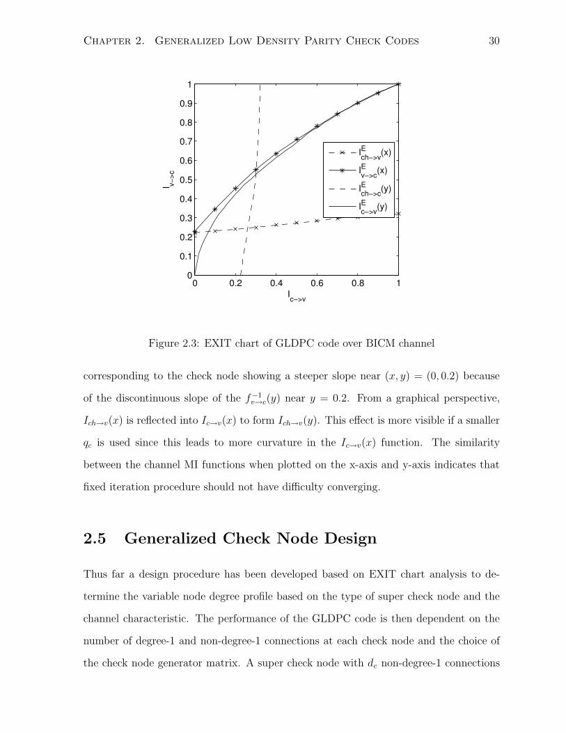
Chapter 2. Generalized Low Density Parity Check Codes 30
0 0.2 0.4 0.6 0.8 10
0.1
0.2
0.3
0.4
0.5
0.6
0.7
0.8
0.9
1
Ic−>v
I v−>c
IEch−>v(x)
IEv−>c(x)
IEch−>c(y)
IEc−>v(y)
Figure 2.3: EXIT chart of GLDPC code over BICM channel
corresponding to the check node showing a steeper slope near (x, y) = (0, 0.2) because
of the discontinuous slope of the f−1v→c(y) near y = 0.2. From a graphical perspective,
Ich→v(x) is reflected into Ic→v(x) to form Ich→v(y). This effect is more visible if a smaller
qc is used since this leads to more curvature in the Ic→v(x) function. The similarity
between the channel MI functions when plotted on the x-axis and y-axis indicates that
fixed iteration procedure should not have difficulty converging.
2.5 Generalized Check Node Design
Thus far a design procedure has been developed based on EXIT chart analysis to de-
termine the variable node degree profile based on the type of super check node and the
channel characteristic. The performance of the GLDPC code is then dependent on the
number of degree-1 and non-degree-1 connections at each check node and the choice of
the check node generator matrix. A super check node with dc non-degree-1 connections
Chapter 2. Generalized Low Density Parity Check Codes 31
and qc degree-1 connections is formed by a (qc + dc, dc − 1) block code with a generator
matrix G = [Ik,P], with the first column of P consisting of all ones. When the number
of degree-1 and non-degree-1 connections has been fixed, what remains is determining
the last qc columns of the parity check matrix P.
EXIT chart can be useful in finding a good super check node generator matrix, espe-
cially since the overall code performance is analyzed using EXIT charts in the previous
section. There are a couple of factors that influence super check node design. The first
is how closely the check node EXIT curve can be matched by repetition code curve. The
mismatched area is direct rate-loss. The second factor has to do with how the check
node EXIT curve shifts with a change in channel SNR and is determined by the number
of channel connections qc. A large value of qc gives rise to a check node MI function
that is sensitive to the channel SNR, so a small power-loss is incurred to open a decod-
ing tunnel of sufficient size to achieve error free transmission for finite packet lengths.
Unfortunately, a large qc value leads to curve matching problems that were pointed out
in [60] and will be further discussed later in this section. In order to balance these two
factors, it is necessary to determine P for different values of dc and qc, simulate the FER
performance for the packet length of interest, and choose the parity check matrix with
the smallest FER.
The super check node in general has two MI functions, with IEc→v = fc→v(I
Iv→c, I
Ich→c)
determining the MI going to the variable nodes and IEc→ch = fc→ch(I
Iv→c, I
Ich→c) determin-
ing the MI going to the channel nodes. For the purposes of designing the check node
generator, only the output IEc→v is considered and not IE
c→ch. For the binary AWGN chan-
nel or MLCM-MSD system, IEc→ch is not used entirely, and for the BICM-IDD system,
the variable node EXIT curve is much steeper than the channel EXIT curve, thus IEc→v
has a significantly larger effect on system performance than IEc→ch. Another simplifying
assumption employed for check node generator design is that the intrinsic channel and
variable node messages are independent, which is strictly the case for the binary AWGN
Chapter 2. Generalized Low Density Parity Check Codes 32
channel. For the BICM-IDD system, the assumption of independent inputs should not
significantly affect the resulting check node parity check matrix if the mapping function
is chosen to minimize symbol message correlation.
A family of K codes can be formed by extending a (dc, dc − 1) single parity check
code through the addition of columns to the parity check matrix in a recursive manner.
The first code in the set has parity check matrix P1 = 1(dc−1)×1. The lth matrix is
formed from the (l − 1)th matrix according to Pl = [Pl−1,pl], where pl ∈ Bdc−1. What
is required is a criterion to determine pl from Pl−1. From the EXIT chart in Figure 2.3,
convergence is predicted if the check node curve stays below the variable node curve.
This suggests that maximizing the area to the right of the check node curve should lead
to a low convergence SNR. One complication is that as the design rate and qc increases,
the check node curve tends to lift away from the y-axis at the origin and cannot be closely
matched by the variable node curve. The area under the check node curve fc→v(y, IIch→c)
near y = 0 is not recoverable by a repetition code, and so the domain of y can be limited
to y ∈ [β 1], 0 < β < 1. Let fEc→v(I
Iv→c, I
Ich→c,P) and fAPP
c→v (IIv→c, I
Ich→c,P) be the check
node extrinsic and a posteriori output, respectively. For a previous parity check matrix
Pl−1, the current parity vector pl can be found using the following selection criterion:
arg maxp∈SAd(Pl−1)
∫ 1
β
fEc→v(y, II
ch→c, [Pl−1,p]) + fAPPc→v (y, II
ch→c, [Pl−1,p])dy (2.19)
where SAd(P) = Bdc−1 − col(P) − cols(Ik) is the set of admissible p vectors and col(X)
represent the set of column vectors forming X. Both the extrinsic and APP functions are
averaged in (2.19). The gap between the APP and extrinsic functions is greatest near the
middle of the [0 1] domain, thus the inclusion of the APP function in (2.19) places more
weight on the area under the extrinsic curve near the center of the domain, which results
in slightly better performance. For a channel message MI of I Ich→c = 0.25, the recursive
application of (2.19) yields a family of check nodes whose transfer characteristics are
shown in Figure 2.4 (left), for dc = 7, qc = [0 . . . 6] and β = 0, 0.5. The parity check
matrices used to generate the first six curves in Figure 2.4 (left) are a subset of the matrix

Chapter 2. Generalized Low Density Parity Check Codes 33
0 0.2 0.4 0.6 0.8 10
0.2
0.4
0.6
0.8
1
IIc−>v
IE v−>c
0 0.2 0.4 0.6 0.8 10
0.2
0.4
0.6
0.8
1
II v−>c
IEc−>v
β=0β=0.5
Figure 2.4: EXIT chart for super check nodes with dc = 7 and qc = [0 . . . 6] (left) and
irregular repetition codes with dv = [2 . . . 8] (right)
in (2.18) for the β = 0.5 case. Shown in Figure 2.4 (right) is the set of repetition code
transfer functions for dv = [2 . . . 8] generated at the same channel MI. One can see that
the check and variable node curves have complementary shapes for the β = 0.5 case, but
the check node curves lift away from the y-axis for the β = 0 case leading to a rate-loss.
In the β = 0.5 case, a super check node EXIT curve can be matched with a low rate
repetition code, provided that the number of degree-1 check node bits is not too large.
The choice of the admissible set of vectors in (2.19) used to generate the kth code in
the family is worth some discussion. Vectors corresponding to the non-degree-1 bits and
previously selected degree-1 bits are removed from the admissible set in (2.19) in order
to minimize the rate-loss in the region near y = 0. The repetition of a non-degree-1 bits
as a degree-1 bits will cause the check node MI function to be more heavily influenced by
IIch→c. Since II
ch→c is unchanged over y, the repetition of a non-degree-1 bit will raise the
check node MI function all over, including the region near y = 0 that is unrecoverable.
Allowing the repetition of degree-1 bits has a similar, but lesser effect.
The family of check node codes generated using (2.19) is dependent on the channel
Chapter 2. Generalized Low Density Parity Check Codes 34
SNR through IIch→c, and so different parity check matrices can be generated that are
suited to various SNR ranges. The check node MI functions fEc→v(I
Iv→c, I
Ich→c,P) and
fEc→ch(I
Iv→c, I
Ich→c,P) can be evaluated using Monte Carlo simulation and tabulated for
different P over the input space IIv→c, I
Ich→c ∈ [0 1]. Using the tabulated values, the
check node MI functions can be efficiently evaluated for an arbitrary I Iv→c, I
Ich→c using
2-dimensional interpolation.
2.6 Code Graph Construction with Cycles
Thus far, GLDPC code design has been discussed without consideration to how the LDPC
code graph is constructed, or how cycles or loops in the graph affect performance. Loops
in the GLDPC graph, or the combined channel and GLDPC code graph, have a negative
effect on BP decoder performance. This is because loops lead to a correlated intrinsic
input and an overconfident extrinsic output that will degrade decoding performance. For
long codes, the code graphs can be efficiently built from randomly constructed graphs
with near capacity achieving performance [16, 18], since the average minimum distance
between nodes in the graph is large. The performance of random code construction is
often improved by removing loops of length 4 in a post-processing step.
When constructing short-to-moderate length codes, more attention has to be paid to
the distribution of loops within the code graph, especially short loops which should be
avoided. The Progressive Edge Growth (PEG) algorithm constructs the code graph in an
edge-by-edge manner with the objective of minimizing the graph girth, or shortest cycle
in the graph [64]. The PEG algorithm maintains a set of connected nodes with minimum
distance dmin. At each step, it forms a spanning tree for the set of connected nodes
with the aim of finding a new connection whose minimum distance to the connected set
is dmin or more. If this is not possible, a connection is made that maximizes the new
dmin. Variations on the PEG algorithm have been proposed [65, 66], that use slightly
Chapter 2. Generalized Low Density Parity Check Codes 35
different selection criteria when there are several candidate nodes with the same dmin.
These modifications to the approach in [64] offer a slight performance improvement in
the high SNR region. The PEG algorithm from [64] has been used to design the code
graphs for the GLDPC codes developed in this chapter.
A graph’s girth is a good indication of the performance gap between finite length code
performance and the theoretical EXIT chart predicted performance under the cycle free
assumption. For a fixed code rate, graph girth for PEG and other construction methods
increases with code length and decreases with both check and variable node degrees. For
a fixed number of information bits, the maximum graph girth increases with the code
rate. To see this, consider an irregular rate r = 0.01 LDPC code of length 1000, with 990
checks, which certainly containing loops of length 4. In comparison, the PEG algorithm
can produce a graph of girth 10, for a r = 0.5 regular LDPC code of the same length.
The relationship between girth and code rate is significant for GLDPC codes that are
based on a higher rate LDPC subcode. The rate r = 0.25 GLDPC design example in
Figure 2.3 is based on a rate R = 0.678 LDPC subcode. For a codeword length of 8000,
the PEG algorithm produces a GLDPC code graph of girth 8, which compares to a girth
of 4 for a similar LDPC code design. In comparison to low rate LDPC codes, GLDPC
codes can be designed with larger girths, and enjoy a smaller performance loss from the
predicted threshold.
The graph produced by the PEG algorithm does not account for loops induced by
channel message correlation under iterative detection and decoding. Correlated extrinsic
channel messages introduce smaller loops in the combined code and channel graph that
cannot be easily avoided using a graph construction procedure like PEG. For example,
consider a rate R = 1/2 LDPC code that is mapped to a symbol with two bits. If the
symbol mapping is treated as a constraint, there are as many constraints as codeword
bits, leading to linearly dependent parity check rows and loops of length four. Although
loops induced by the channel graph cannot be avoided, its effect on the BP decoder
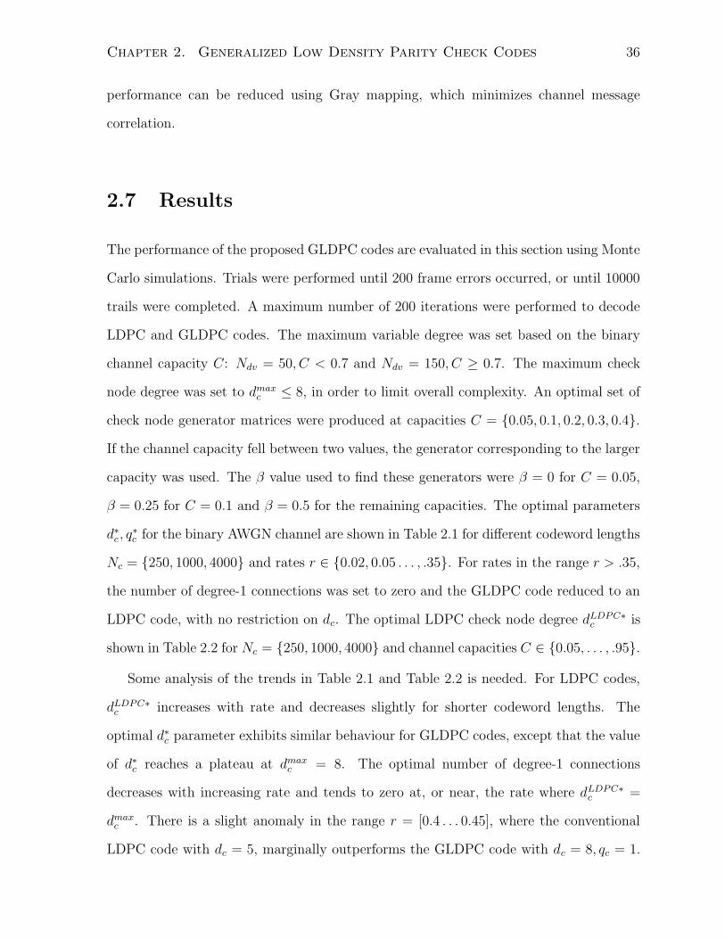
Chapter 2. Generalized Low Density Parity Check Codes 36
performance can be reduced using Gray mapping, which minimizes channel message
correlation.
2.7 Results
The performance of the proposed GLDPC codes are evaluated in this section using Monte
Carlo simulations. Trials were performed until 200 frame errors occurred, or until 10000
trails were completed. A maximum number of 200 iterations were performed to decode
LDPC and GLDPC codes. The maximum variable degree was set based on the binary
channel capacity C: Ndv = 50, C < 0.7 and Ndv = 150, C ≥ 0.7. The maximum check
node degree was set to dmaxc ≤ 8, in order to limit overall complexity. An optimal set of
check node generator matrices were produced at capacities C = 0.05, 0.1, 0.2, 0.3, 0.4.
If the channel capacity fell between two values, the generator corresponding to the larger
capacity was used. The β value used to find these generators were β = 0 for C = 0.05,
β = 0.25 for C = 0.1 and β = 0.5 for the remaining capacities. The optimal parameters
d∗c , q
∗c for the binary AWGN channel are shown in Table 2.1 for different codeword lengths
Nc = 250, 1000, 4000 and rates r ∈ 0.02, 0.05 . . . , .35. For rates in the range r > .35,
the number of degree-1 connections was set to zero and the GLDPC code reduced to an
LDPC code, with no restriction on dc. The optimal LDPC check node degree dLDPC∗c is
shown in Table 2.2 for Nc = 250, 1000, 4000 and channel capacities C ∈ 0.05, . . . , .95.
Some analysis of the trends in Table 2.1 and Table 2.2 is needed. For LDPC codes,
dLDPC∗c increases with rate and decreases slightly for shorter codeword lengths. The
optimal d∗c parameter exhibits similar behaviour for GLDPC codes, except that the value
of d∗c reaches a plateau at dmax
c = 8. The optimal number of degree-1 connections
decreases with increasing rate and tends to zero at, or near, the rate where dLDPC∗c =
dmaxc . There is a slight anomaly in the range r = [0.4 . . . 0.45], where the conventional
LDPC code with dc = 5, marginally outperforms the GLDPC code with dc = 8, qc = 1.
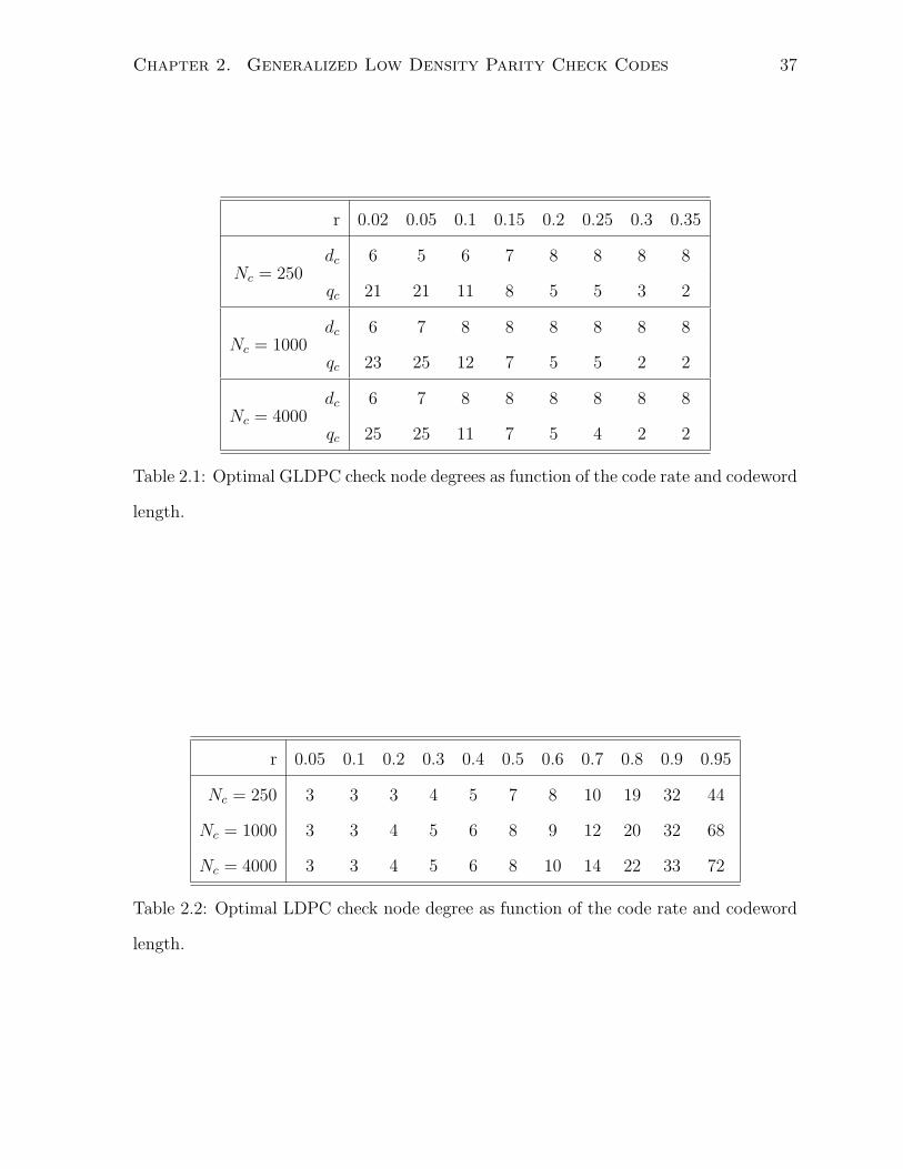
Chapter 2. Generalized Low Density Parity Check Codes 37
r 0.02 0.05 0.1 0.15 0.2 0.25 0.3 0.35
Nc = 250dc 6 5 6 7 8 8 8 8
qc 21 21 11 8 5 5 3 2
Nc = 1000dc 6 7 8 8 8 8 8 8
qc 23 25 12 7 5 5 2 2
Nc = 4000dc 6 7 8 8 8 8 8 8
qc 25 25 11 7 5 4 2 2
Table 2.1: Optimal GLDPC check node degrees as function of the code rate and codeword
length.
r 0.05 0.1 0.2 0.3 0.4 0.5 0.6 0.7 0.8 0.9 0.95
Nc = 250 3 3 3 4 5 7 8 10 19 32 44
Nc = 1000 3 3 4 5 6 8 9 12 20 32 68
Nc = 4000 3 3 4 5 6 8 10 14 22 33 72
Table 2.2: Optimal LDPC check node degree as function of the code rate and codeword
length.
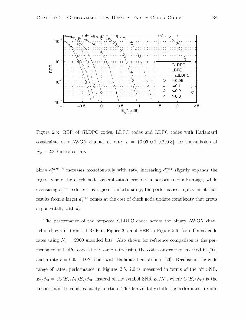
Chapter 2. Generalized Low Density Parity Check Codes 38
−1 −0.5 0 0.5 1 1.5 2 2.510−4
10−3
10−2
10−1
BE
R
Eb/N0(dB)
GLDPCLDPCHadLDPCr=0.05r=0.1r=0.2r=0.3
Figure 2.5: BER of GLDPC codes, LDPC codes and LDPC codes with Hadamard
constraints over AWGN channel at rates r = 0.05, 0.1, 0.2, 0.3 for transmission of
Nu = 2000 uncoded bits
Since dLDPC∗c increases monotonically with rate, increasing dmax
c slightly expands the
region where the check node generalization provides a performance advantage, while
decreasing dmaxc reduces this region. Unfortunately, the performance improvement that
results from a larger dmaxc comes at the cost of check node update complexity that grows
exponentially with dc.
The performance of the proposed GLDPC codes across the binary AWGN chan-
nel is shown in terms of BER in Figure 2.5 and FER in Figure 2.6, for different code
rates using Nu = 2000 uncoded bits. Also shown for reference comparison is the per-
formance of LDPC code at the same rates using the code construction method in [20],
and a rate r = 0.05 LDPC code with Hadamard constraints [60]. Because of the wide
range of rates, performance in Figures 2.5, 2.6 is measured in terms of the bit SNR,
Eb/N0 = 2C(Es/N0)Es/N0, instead of the symbol SNR Es/N0, where C(Es/N0) is the
unconstrained channel capacity function. This horizontally shifts the performance results
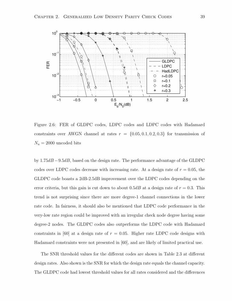
Chapter 2. Generalized Low Density Parity Check Codes 39
−1 −0.5 0 0.5 1 1.5 2 2.510−3
10−2
10−1
100
FER
Eb/N0(dB)
GLDPCLDPCHadLDPCr=0.05r=0.1r=0.2r=0.3
Figure 2.6: FER of GLDPC codes, LDPC codes and LDPC codes with Hadamard
constraints over AWGN channel at rates r = 0.05, 0.1, 0.2, 0.3 for transmission of
Nu = 2000 uncoded bits
by 1.75dB−9.5dB, based on the design rate. The performance advantage of the GLDPC
codes over LDPC codes decrease with increasing rate. At a design rate of r = 0.05, the
GLDPC code boasts a 2dB-2.5dB improvement over the LDPC codes depending on the
error criteria, but this gain is cut down to about 0.5dB at a design rate of r = 0.3. This
trend is not surprising since there are more degree-1 channel connections in the lower
rate code. In fairness, it should also be mentioned that LDPC code performance in the
very-low rate region could be improved with an irregular check node degree having some
degree-2 nodes. The GLDPC codes also outperforms the LDPC code with Hadamard
constraints in [60] at a design rate of r = 0.05. Higher rate LDPC code designs with
Hadamard constraints were not presented in [60], and are likely of limited practical use.
The SNR threshold values for the different codes are shown in Table 2.3 at different
design rates. Also shown is the SNR for which the design rate equals the channel capacity.
The GLDPC code had lowest threshold values for all rates considered and the differences
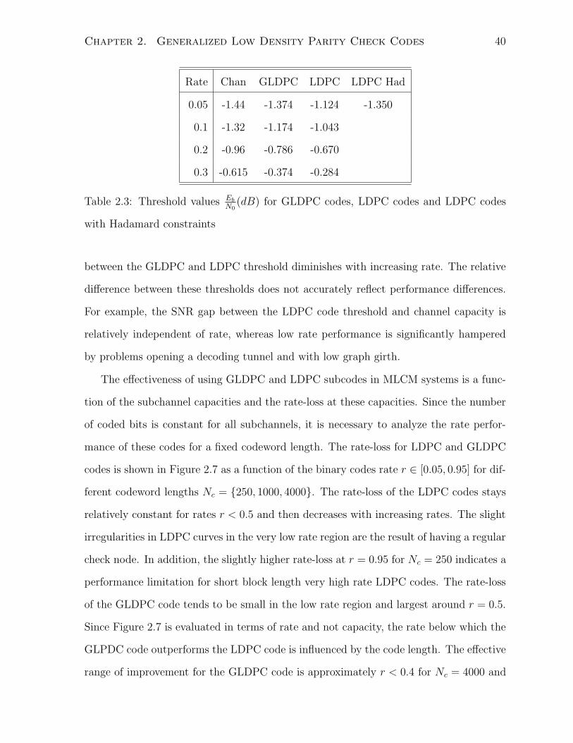
Chapter 2. Generalized Low Density Parity Check Codes 40
Rate Chan GLDPC LDPC LDPC Had
0.05 -1.44 -1.374 -1.124 -1.350
0.1 -1.32 -1.174 -1.043
0.2 -0.96 -0.786 -0.670
0.3 -0.615 -0.374 -0.284
Table 2.3: Threshold values Eb
N0(dB) for GLDPC codes, LDPC codes and LDPC codes
with Hadamard constraints
between the GLDPC and LDPC threshold diminishes with increasing rate. The relative
difference between these thresholds does not accurately reflect performance differences.
For example, the SNR gap between the LDPC code threshold and channel capacity is
relatively independent of rate, whereas low rate performance is significantly hampered
by problems opening a decoding tunnel and with low graph girth.
The effectiveness of using GLDPC and LDPC subcodes in MLCM systems is a func-
tion of the subchannel capacities and the rate-loss at these capacities. Since the number
of coded bits is constant for all subchannels, it is necessary to analyze the rate perfor-
mance of these codes for a fixed codeword length. The rate-loss for LDPC and GLDPC
codes is shown in Figure 2.7 as a function of the binary codes rate r ∈ [0.05, 0.95] for dif-
ferent codeword lengths Nc = 250, 1000, 4000. The rate-loss of the LDPC codes stays
relatively constant for rates r < 0.5 and then decreases with increasing rates. The slight
irregularities in LDPC curves in the very low rate region are the result of having a regular
check node. In addition, the slightly higher rate-loss at r = 0.95 for Nc = 250 indicates a
performance limitation for short block length very high rate LDPC codes. The rate-loss
of the GLDPC code tends to be small in the low rate region and largest around r = 0.5.
Since Figure 2.7 is evaluated in terms of rate and not capacity, the rate below which the
GLPDC code outperforms the LDPC code is influenced by the code length. The effective
range of improvement for the GLDPC code is approximately r < 0.4 for Nc = 4000 and
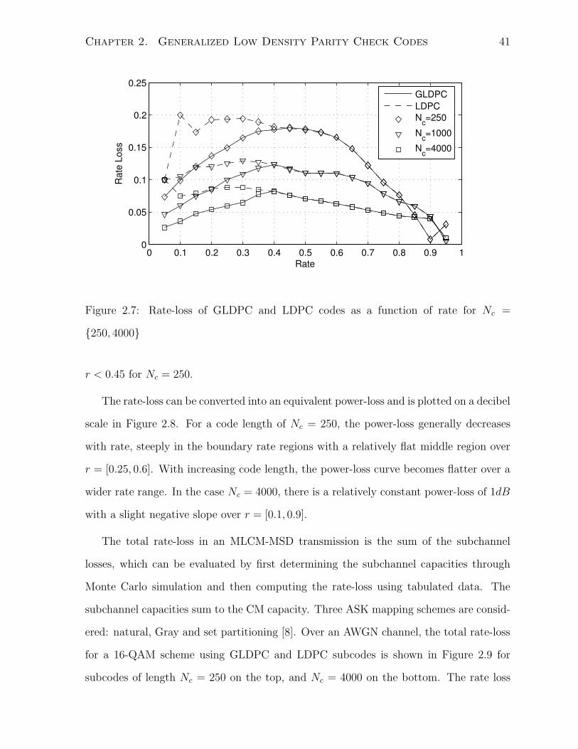
Chapter 2. Generalized Low Density Parity Check Codes 41
0 0.1 0.2 0.3 0.4 0.5 0.6 0.7 0.8 0.9 10
0.05
0.1
0.15
0.2
0.25
Rat
e Lo
ss
Rate
GLDPCLDPCNc=250
Nc=1000
Nc=4000
Figure 2.7: Rate-loss of GLDPC and LDPC codes as a function of rate for Nc =
250, 4000
r < 0.45 for Nc = 250.
The rate-loss can be converted into an equivalent power-loss and is plotted on a decibel
scale in Figure 2.8. For a code length of Nc = 250, the power-loss generally decreases
with rate, steeply in the boundary rate regions with a relatively flat middle region over
r = [0.25, 0.6]. With increasing code length, the power-loss curve becomes flatter over a
wider rate range. In the case Nc = 4000, there is a relatively constant power-loss of 1dB
with a slight negative slope over r = [0.1, 0.9].
The total rate-loss in an MLCM-MSD transmission is the sum of the subchannel
losses, which can be evaluated by first determining the subchannel capacities through
Monte Carlo simulation and then computing the rate-loss using tabulated data. The
subchannel capacities sum to the CM capacity. Three ASK mapping schemes are consid-
ered: natural, Gray and set partitioning [8]. Over an AWGN channel, the total rate-loss
for a 16-QAM scheme using GLDPC and LDPC subcodes is shown in Figure 2.9 for
subcodes of length Nc = 250 on the top, and Nc = 4000 on the bottom. The rate loss
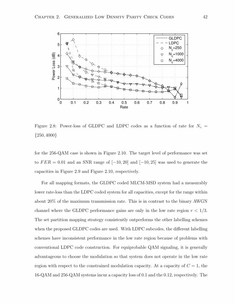
Chapter 2. Generalized Low Density Parity Check Codes 42
0 0.1 0.2 0.3 0.4 0.5 0.6 0.7 0.8 0.9 10
1
2
3
4
5
6
Rate
Pow
er L
oss
(dB
)
GLDPCLDPCNc=250
Nc=1000
Nc=4000
Figure 2.8: Power-loss of GLDPC and LDPC codes as a function of rate for Nc =
250, 4000
for the 256-QAM case is shown in Figure 2.10. The target level of performance was set
to FER = 0.01 and an SNR range of [−10, 20] and [−10, 25] was used to generate the
capacities in Figure 2.9 and Figure 2.10, respectively.
For all mapping formats, the GLDPC coded MLCM-MSD system had a measurably
lower rate-loss than the LDPC coded system for all capacities, except for the range within
about 20% of the maximum transmission rate. This is in contrast to the binary AWGN
channel where the GLDPC performance gains are only in the low rate region r < 1/3.
The set partition mapping strategy consistently outperforms the other labelling schemes
when the proposed GLDPC codes are used. With LDPC subcodes, the different labelling
schemes have inconsistent performance in the low rate region because of problems with
conventional LDPC code construction. For equiprobable QAM signaling, it is generally
advantageous to choose the modulation so that system does not operate in the low rate
region with respect to the constrained modulation capacity. At a capacity of C = 1, the
16-QAM and 256-QAM systems incur a capacity loss of 0.1 and the 0.12, respectively. The

Chapter 2. Generalized Low Density Parity Check Codes 43
0 0.2 0.4 0.6 0.8 1 1.2 1.4 1.6 1.8 20
0.1
0.2
0.3
0.4
Rat
e−lo
ss
Rate−Loss, 16QAM, Nc=250
0 0.2 0.4 0.6 0.8 1 1.2 1.4 1.6 1.8 20
0.05
0.1
0.15
0.2
CCM
Rat
e−lo
ss
Rate−Loss, 16QAM, Nc=4000
Nc=GLDPC
Nc=LDPC
NatGraySet Partition
Figure 2.9: Rate-loss for 16-QAM MLCM-MSD transmission using GLDPC (top) and
LDPC (bottom) subcodes and different labelling functions for packet lengths of Nc =
250, 4000

Chapter 2. Generalized Low Density Parity Check Codes 44
0 0.5 1 1.5 2 2.5 3 3.5 40
0.2
0.4
0.6
0.8
Rat
e−lo
ss
Rate−Loss, 256QAM, Nc=250
0 0.5 1 1.5 2 2.5 3 3.5 40
0.1
0.2
0.3
0.4
CCM
Rat
e−lo
ss
Rate−Loss, 256QAM, Nc=4000
Nc=GLDCP
Nc=LDPC
NatGraySet Partition
Figure 2.10: Rate-loss for 256-QAM MLCM-MSD transmission using GLDPC (top) and
LDPC (bottom) subcodes and different labelling functions for packet lengths of Nc =
250, 4000

Chapter 2. Generalized Low Density Parity Check Codes 45
0.5 1 1.5 2 2.5 3 3.5 4
10−3
10−2
10−1
100
Eb/N0(dB)
FER
GLDPCLDPCr=1r=1,Modr=2
Figure 2.11: FER of LDPC and GLDPC coded MLCM-MSD systems over AWGN chan-
nel using 16-QAM
larger loss in the 256-QAM case results from low capacity subchannels that lead to zero-
rate subcodes. A zero-rate subcode is equivalent to encoding a pseudo-random binary
sequence which is quite power inefficient, since this subchannel increases the symbol
energy without providing any additional transmission rate.
The performance of the 16-QAM MLCM-MSD system using LDPC and GLDPC sub-
codes is shown in Figure 2.11 for transmissions of Ns = 2000 symbols with a throughput
of r = 1, 2 bits per channel use. The use of GLDPC codes improved system performance
by 0.7dB in the r = 1 system and 0.2dB in the r = 2 system. In the r = 1 case,
system performance was improved when the rate of the first subcode was reduced by
0.012, shown with a label ’Mod’ in Figure 2.11. Similar rate reduction did not produce
appreciable performance improvement in the r = 2 system.
The need for a rate adjustment in the rate r = 1 system stems from non-Gaussianity in
the channel node message densities when set partitioning labelling is used. Consider de-
tecting the least significant bit first in a natural 4-ASK modulation, and let −3,−1, 1, 3
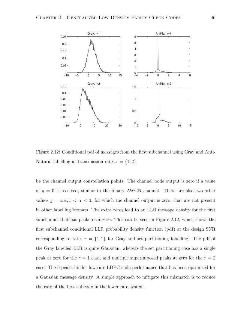
Chapter 2. Generalized Low Density Parity Check Codes 46
−10 −5 0 5 10 150
0.05
0.1
0.15
0.2
0.25Gray, r=1
−4 −2 0 2 4 60
1
2
3
4
5
6AntiNat, r=1
−10 0 10 20 300
0.02
0.04
0.06
0.08
0.1
0.12Gray, r=2
−10 −5 0 5 10 150
0.5
1
1.5AntiNat, r=2
Figure 2.12: Conditional pdf of messages from the first subchannel using Gray and Anti-
Natural labelling at transmission rates r = 1, 2
be the channel output constellation points. The channel node output is zero if a value
of y = 0 is received, similar to the binary AWGN channel. There are also two other
values y = ±α, 1 < α < 3, for which the channel output is zero, that are not present
in other labelling formats. The extra zeros lead to an LLR message density for the first
subchannel that has peaks near zero. This can be seen in Figure 2.12, which shows the
first subchannel conditional LLR probability density function (pdf) at the design SNR
corresponding to rates r = 1, 2 for Gray and set partitioning labelling. The pdf of
the Gray labelled LLR is quite Gaussian, whereas the set partitioning case has a single
peak at zero for the r = 1 case, and multiple superimposed peaks at zero for the r = 2
case. These peaks hinder low rate LDPC code performance that has been optimized for
a Gaussian message density. A simple approach to mitigate this mismatch is to reduce
the rate of the first subcode in the lower rate system.
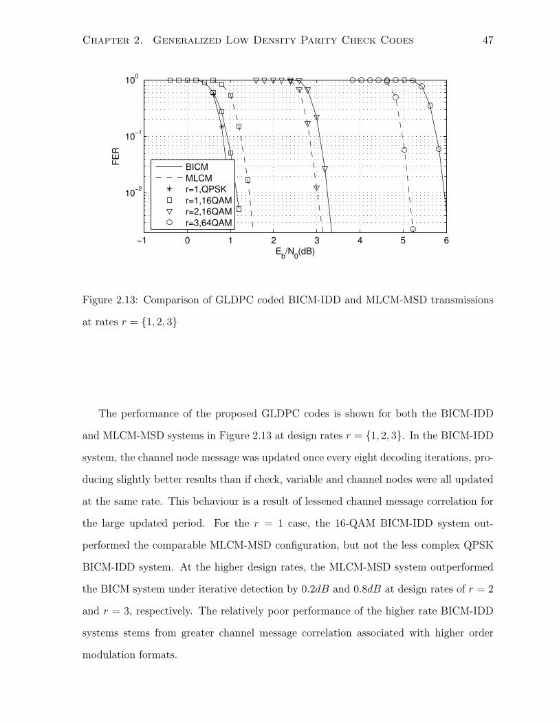
Chapter 2. Generalized Low Density Parity Check Codes 47
−1 0 1 2 3 4 5 6
10−2
10−1
100
FER
Eb/N0(dB)
BICMMLCMr=1,QPSKr=1,16QAMr=2,16QAMr=3,64QAM
Figure 2.13: Comparison of GLDPC coded BICM-IDD and MLCM-MSD transmissions
at rates r = 1, 2, 3
The performance of the proposed GLDPC codes is shown for both the BICM-IDD
and MLCM-MSD systems in Figure 2.13 at design rates r = 1, 2, 3. In the BICM-IDD
system, the channel node message was updated once every eight decoding iterations, pro-
ducing slightly better results than if check, variable and channel nodes were all updated
at the same rate. This behaviour is a result of lessened channel message correlation for
the large updated period. For the r = 1 case, the 16-QAM BICM-IDD system out-
performed the comparable MLCM-MSD configuration, but not the less complex QPSK
BICM-IDD system. At the higher design rates, the MLCM-MSD system outperformed
the BICM system under iterative detection by 0.2dB and 0.8dB at design rates of r = 2
and r = 3, respectively. The relatively poor performance of the higher rate BICM-IDD
systems stems from greater channel message correlation associated with higher order
modulation formats.

Chapter 2. Generalized Low Density Parity Check Codes 48
2.8 Summary
In this chapter, a set of generalized irregular LDPC codes is developed by extending
single parity check codes with additional parity bits that are connected directly to the
channel without repetition. These codes are aimed at the low rate R < 1/3 region where
conventional LDPC code have low girth problems and require a large power loss to open a
decoding tunnel. The generalization of the check node with degree-1 channel connections
increases the area under the check node EXIT curve and the rate of the LDPC subcode.
The use of a higher rate LDPC subcode mitigates adverse low rate effects. In coded
modulation systems, the proposed codes improve MLCM-MSD performance over a wide
range of rates, when set partitioning labelling is used. The GLDPC coded MLCM-MSD
system also outperforms comparable BICM-IDD systems for higher order modulation
formats.

Chapter 3
Irregular Convolutional Coding
The GLDPC codes developed in the last chapter were rendered ineffective under iterative
detection and decoding because of message correlation introduced by the multiple serially
concatenated structure. BICM transmissions are usually coded with a single outer code
such as a convolutional code, or a parallel concatenated outer code such as a turbo code.
This chapter develops an irregular convolutional coding structure for use as an outer code
in a BICM system. These codes can be designed to suit different mapping choices and
channel conditions.
3.1 Introduction
Since the discovery of turbo codes [13, 14], iterative decoding of concatenated convolu-
tional codes has been the subject of much research interest and a part of many existing
wireless standards. In comparison to LDPC codes, turbo codes perform better over short
blocks and slightly worse for longer transmissions. In coded modulation applications,
turbo codes and convolutional codes are widely used in BICM-IDD systems with itera-
tive detection and decoding [67, 68, 69, 70, 71, 52, 72]. The outer code design is influenced
by the channel, mapping, and modulation.
EXIT charts are a useful outer code design tool in BICM-IDD systems. Under IDD
49

Chapter 3. Irregular Convolutional Coding 50
processing, messages are passed between the outer decoder and the channel detector.
The evolution of mutual information for these messages can be represented on an EXIT
chart, and the code design problem becomes one of finding a code with an EXIT curve
that matches the channel EXIT curve [72, 21]. Gray mapping has an almost horizontal
EXIT curve for many channels and is generally well paired with a turbo code outer code.
For other mapping formats, it is more difficult to find an off-the-shelf outer code with
good EXIT curve matching properties.
There are two approaches to mitigate capacity loss due to EXIT curve mismatch
that can be employed separately or together. The first to use an irregular outer code
to influence the decoder EXIT curve, and the second is to control the shape of the
decoder EXIT curve through a multi-dimensional mapping function. The latter approach
is used in [67, 68, 69, 73, 74, 52, 40, 42], which applies the binary switching algorithm
to optimize the detector EXIT curve. Alternatively, the decoder EXIT curve can be
controlled through puncturing. In [72, 75, 76], an irregular convolutional code is formed
using a set of subcodes produced from a convolutional mother code and a set of rate
compatible puncture patterns. For turbo codes, EXIT curve shape can be manipulated to
some extent using regular repetition and puncturing of the systematic or parity bits [77].
This chapter extends the work on irregular convolutional codes in [72] by introducing
irregularity through generators of different memory. In [72], a single low-rate mother code
is used with a rate compatible set of puncture patterns to produce a set of subcodes.
These subcodes can be represented as a family of non-intersecting ‘S’ shaped EXIT
curves, where each curve consists of two flat regions with a steeply sloped transition
region in the middle. The set of EXIT curves are approximately a horizontal shift of
each other. The use of irregular puncturing alone allow some flexibility to design a
decoder EXIT to match the channel and mapper characteristic. More efficient codes can
be designed with an expanded set of subcodes that differ in terms of both horizontal
alignment and steepness of the transition region. The steepness of the transition region
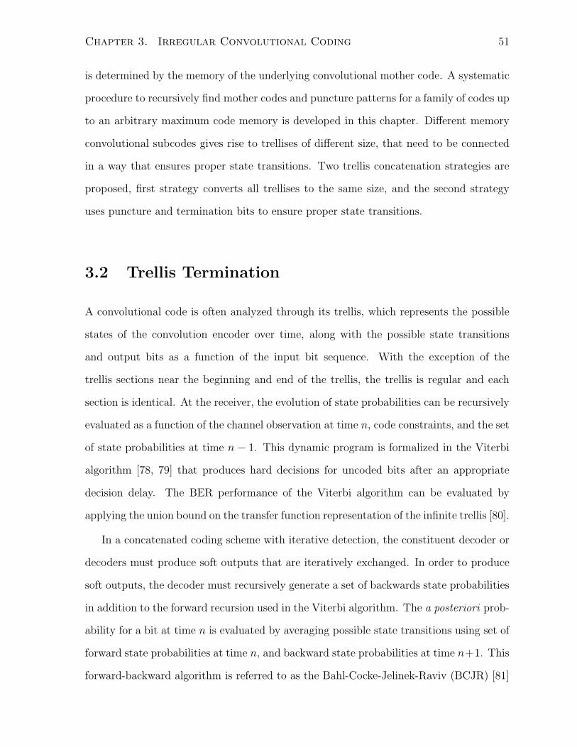
Chapter 3. Irregular Convolutional Coding 51
is determined by the memory of the underlying convolutional mother code. A systematic
procedure to recursively find mother codes and puncture patterns for a family of codes up
to an arbitrary maximum code memory is developed in this chapter. Different memory
convolutional subcodes gives rise to trellises of different size, that need to be connected
in a way that ensures proper state transitions. Two trellis concatenation strategies are
proposed, first strategy converts all trellises to the same size, and the second strategy
uses puncture and termination bits to ensure proper state transitions.
3.2 Trellis Termination
A convolutional code is often analyzed through its trellis, which represents the possible
states of the convolution encoder over time, along with the possible state transitions
and output bits as a function of the input bit sequence. With the exception of the
trellis sections near the beginning and end of the trellis, the trellis is regular and each
section is identical. At the receiver, the evolution of state probabilities can be recursively
evaluated as a function of the channel observation at time n, code constraints, and the set
of state probabilities at time n − 1. This dynamic program is formalized in the Viterbi
algorithm [78, 79] that produces hard decisions for uncoded bits after an appropriate
decision delay. The BER performance of the Viterbi algorithm can be evaluated by
applying the union bound on the transfer function representation of the infinite trellis [80].
In a concatenated coding scheme with iterative detection, the constituent decoder or
decoders must produce soft outputs that are iteratively exchanged. In order to produce
soft outputs, the decoder must recursively generate a set of backwards state probabilities
in addition to the forward recursion used in the Viterbi algorithm. The a posteriori prob-
ability for a bit at time n is evaluated by averaging possible state transitions using set of
forward state probabilities at time n, and backward state probabilities at time n+1. This
forward-backward algorithm is referred to as the Bahl-Cocke-Jelinek-Raviv (BCJR) [81]
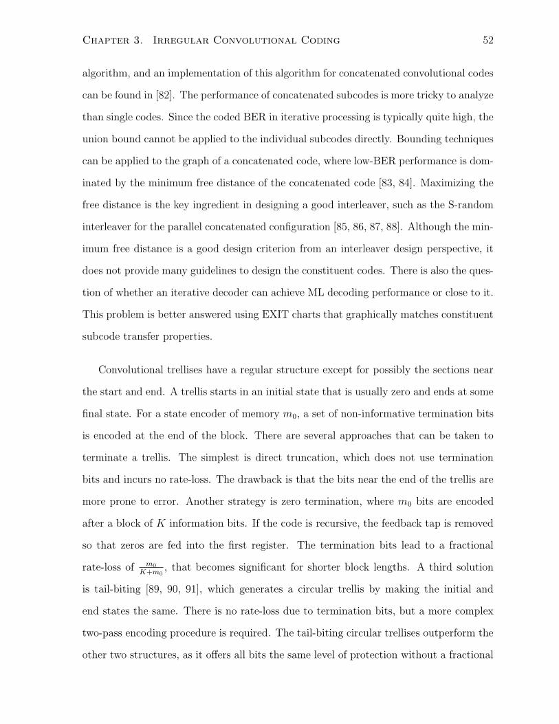
Chapter 3. Irregular Convolutional Coding 52
algorithm, and an implementation of this algorithm for concatenated convolutional codes
can be found in [82]. The performance of concatenated subcodes is more tricky to analyze
than single codes. Since the coded BER in iterative processing is typically quite high, the
union bound cannot be applied to the individual subcodes directly. Bounding techniques
can be applied to the graph of a concatenated code, where low-BER performance is dom-
inated by the minimum free distance of the concatenated code [83, 84]. Maximizing the
free distance is the key ingredient in designing a good interleaver, such as the S-random
interleaver for the parallel concatenated configuration [85, 86, 87, 88]. Although the min-
imum free distance is a good design criterion from an interleaver design perspective, it
does not provide many guidelines to design the constituent codes. There is also the ques-
tion of whether an iterative decoder can achieve ML decoding performance or close to it.
This problem is better answered using EXIT charts that graphically matches constituent
subcode transfer properties.
Convolutional trellises have a regular structure except for possibly the sections near
the start and end. A trellis starts in an initial state that is usually zero and ends at some
final state. For a state encoder of memory m0, a set of non-informative termination bits
is encoded at the end of the block. There are several approaches that can be taken to
terminate a trellis. The simplest is direct truncation, which does not use termination
bits and incurs no rate-loss. The drawback is that the bits near the end of the trellis are
more prone to error. Another strategy is zero termination, where m0 bits are encoded
after a block of K information bits. If the code is recursive, the feedback tap is removed
so that zeros are fed into the first register. The termination bits lead to a fractional
rate-loss of m0
K+m0, that becomes significant for shorter block lengths. A third solution
is tail-biting [89, 90, 91], which generates a circular trellis by making the initial and
end states the same. There is no rate-loss due to termination bits, but a more complex
two-pass encoding procedure is required. The tail-biting circular trellises outperform the
other two structures, as it offers all bits the same level of protection without a fractional
Chapter 3. Irregular Convolutional Coding 53
rate-loss.
As tail-biting trellises perform better than terminated trellises, it is worth discussing
the former in some detail. A convolutional code can be represented using state space
equations:
xn+1 = Axn + Bun
yn = Cxn + Dun (3.1)
where xn ∈ Bm0 is the state vector at time n, un ∈ B
k0 is the input vector with k0 = 1
for binary convolutional subcodes, and parameters A,B,C,D are binary matrices that
represent the convolutional code constraints. For a memory m0 = 2 convolutional code
with recursive systematic generator g = [7 5](Octal) shown in Figure 3.1, the state-space
parameters take on values
A =
0 1
1 1
, B = 1, C =
0 0
1 0
, D =
1
0
and generate a trellis also shown in the figure. The solution to (3.1) is evaluated at time
n as
xn = x[zi]n + x[zs]
n = ATx0 +n−1∑
m=0
An−1−mBuTmum (3.2)
which is the superposition of a zero-input solution x[zi]n generated by the condition ui =
0 ∀i, and a zero-state solution x[zs]n generated from the initial state x0 = 0. If a trellis
circularity is imposed, the state after the last bit is encoded must be the same as the
initial state. Enforcing the condition xN = x0 for a block of N uncoded bits yields the
constraint equation,(
AN + Im0
)
x0 = x[zs]n (3.3)
The initial state can be evaluated as the solution to (3.3) provided that the generator is
chosen so that the matrix(
AN + Im0
)
is invertible. Circular trellises cannot always be
found at certain block lengths, such as lengths that are divisible by three [92, 93]. If the
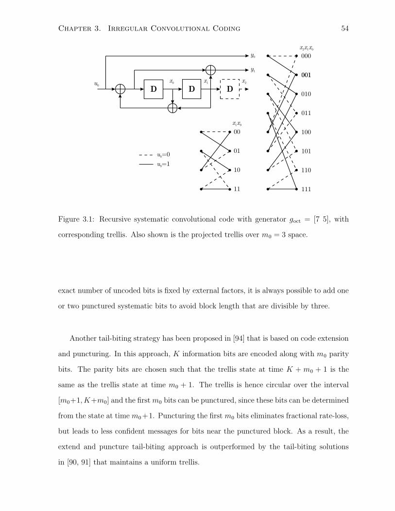
Chapter 3. Irregular Convolutional Coding 54
D
x0
D D
x1u
0
x2
y0
y1
x1x
0
00
01
10
11
x x2 0x
1
001
010
011
001
000
u0=0
u0=1
101
110
111
100
Figure 3.1: Recursive systematic convolutional code with generator goct = [7 5], with
corresponding trellis. Also shown is the projected trellis over m0 = 3 space.
exact number of uncoded bits is fixed by external factors, it is always possible to add one
or two punctured systematic bits to avoid block length that are divisible by three.
Another tail-biting strategy has been proposed in [94] that is based on code extension
and puncturing. In this approach, K information bits are encoded along with m0 parity
bits. The parity bits are chosen such that the trellis state at time K + m0 + 1 is the
same as the trellis state at time m0 + 1. The trellis is hence circular over the interval
[m0+1, K+m0] and the first m0 bits can be punctured, since these bits can be determined
from the state at time m0 +1. Puncturing the first m0 bits eliminates fractional rate-loss,
but leads to less confident messages for bits near the punctured block. As a result, the
extend and puncture tail-biting approach is outperformed by the tail-biting solutions
in [90, 91] that maintains a uniform trellis.

Chapter 3. Irregular Convolutional Coding 55
3.3 Irregular Trellis Concatenation
In an irregular convolutional code, each convolution subcode generates different trellis
sections with different numbers of states. We assume that all trellis sections generated
from one mother code are grouped together in a contiguous block, and that there is
up to one mother code of a given memory. As the decoder complexity is a function of
code memory, let M be the maximum code memory and let αm be the number of trellis
sections of memory m. Unless otherwise stated, a natural ordering of trellis blocks is
assumed based on ascending code memory.
There are two approaches to connecting trellises of different sizes: convert all the trel-
lises to the same size, or using termination and puncture bits to control trellis transitions.
The constant trellis size strategy is an extension of the tail-biting solution in [90, 91],
while the variable trellis size approach is based on the extend and puncture tail-biting
solution in [94]. Each strategy has its relative strengths and weaknesses that depend on
packet length.
A constant size trellis can be formed by recursively representing a trellis of size 2m
within a trellis of size 2m+1, until all trellises have the maximum size. Consider projecting
the g = [7 5]oct, m = 2 convolutional code in Figure 3.1 onto an m = 3 state-space by
adding an additional most significant bit. The output is unaffected by the additional bit,
and the new state bit sm−1 follows the most significant state bit sm−2, as can be seen in
the enlarged projected trellis, also shown in Figure 3.1. Subcodes can be converted to
a common memory M so that all the trellis sections have size 2M . Over this modified
trellis, the BCJR algorithm from [82] can be applied with constraints that are based on
the time-varying state-space equations. The state-space equations in (3.1) can be applied
with vector dimensional agreement by replacing the constant parameters A,B,C,D with
time-varying parameters An, Bn, Cn, Dn that are determined by the subcodes used to
generate the nth trellis section. Also, let the parameters An, Bn, Cn, Dn take on values
Am,Bm,Cm,Dm if the nth trellis section is generated from a subcode having memory m.
Chapter 3. Irregular Convolutional Coding 56
For an irregular convolutional code, enforcing the condition of trellis circularity xN = x0,
yields a constraint equation
(AαMM × . . .×Aα1
1 + IM)x0 = x[zs]n (3.4)
where the Am is defined as
Am =
0M×1 IM−1
01×M−m fbm
with fbm being the binary feedback vector for the mth subcode. The correct value of the
initial state x0 can be found from (3.4) through matrix inversion, since the matrix on the
right hand side of (3.4) in typically non-singular. If an integer solution to (3.3) is not
found, then a circular trellis cannot be formed. Since the matrix (AαMM × . . .×Aα1
1 + IM)
is typically singular, it is possible to have an integer solution to (3.3) for some uncoded
bit sequences and not for others. Several candidate sequences must be tested before
declaring a trellis circular.
If an irregular trellis is found to be non-circular, there are a couple of adjustments that
can be made to bring about circularity. Since matrix multiplication is not commutative,
the order of the trellis blocks influences the circularity of the trellis. If a natural trellis
order does not produce a circular trellis, other orderings can be randomly generated,
thereby changing the order of the Am matrices in (3.3). If a circular trellis cannot be
found by reordering, the number of trellis sections of one mother code can be incremented
and another one decremented, choosing mother codes randomly. Reordering can then be
applied on the modified trellis.
The variable sized trellis can be formed by connecting different size trellises with a
judicious use of puncture and termination bits. An arbitrary state in a trellis of size
2m can be reached from the 0 state after m bits, and is determined by a uniquely bit
sequence for all one-to-one codes. These bits can be punctured as is done in [94], since
the bit values are represented in the state. Now consider two adjacent trellises, the first
Chapter 3. Irregular Convolutional Coding 57
of size m1 and the second of size m2 with m2 > m1. The first m2 − m1 bits in the
second trellis can be punctured since the states in these sections only have one valid
state transition. Consider ordering trellis in increasing order of memory with mmin,M
being the minimum and maximum memory, and encoding K information bits from state-
zero, and M termination bits. The first mmin are punctured and the last M termination
bits are used to set the final state equal to the state at time mmin. This ensures trellis
circularity. There are additionally M −mmin bits at the beginning of each larger trellis
block that are also punctured. This eliminates fractional rate-loss since a total of M bits
are punctured, equaling number of terminations bits.
Comparing the variable and fixed trellis size construction approaches, each has its
relative merit. Puncturing coded bits reduces the average channel message mutual infor-
mation per bit and leads to a fractional capacity loss for short packets. The fixed trellis
size solution has a weak bits near high-to-low memory transitions. This is because last
few bits of the longer memory code are not part shorter memory code feedback loop,
leading to an error floor and poorer longer packet performance.
3.4 Irregular Code Design using EXIT Charts
A convolutional outer code can be serially concatenated with a wide range of different
types of inner codes, the most obvious being another convolutional code. A serially
concatenated convolutional code can be designed to perform within 0.1dB of the Shannon
capacity using a regular outer code and code doping strategy with two inner codes [95].
Unfortunately, serially concatenated convolutional codes do not outperform turbo codes
for short block lengths, despite having a lower SNR convergence threshold. In addition,
serially concatenated convolutional codes and LDPC codes have approximately the same
performance for large block length, but the former typically incurs greater decoder latency
because of the serial nature of trellis decoding.
Chapter 3. Irregular Convolutional Coding 58
The main application for serial concatenated convolutional codes is in BICM-IDD
systems, where the channel detector acts as an inner decoder. One may be tempted to
apply further a serially concatenated code to form a triple concatenated code with the
channel acting as the innermost code. In order to avoid a capacity loss [72], the middle
code must be of unity rate which significantly increases interleaver message correlation.
Since the inner and outer interleavers are the same size, the inner interleaver cannot
provide any additional spreading than the outer interleaver alone. The negative effect of
the inner interleaver becomes more apparent for correlated symbol mappings, although
the triple code concatenated structure should be avoided altogether if possible. A similar
problem is discussed in Chapter 2 with respect to GLDPC coded BICM-IDD system,
where the middle repetition code node is sensitive to channel message correlation.
The BICM channel has an EXIT curve shape that is influenced by the mapping and
physical channel, and whose area approximates the CM channel capacity. The outer code
is designed to match the reflected detector EXIT curve. As the outer code is composed
of a set of convolutional subcodes, understanding the relationship between EXIT curve
shape and the choice of generator polynomial is of key importance. Following the work
in [72], we consider RSC mother codes. All one-to-one RSC code realizations have an
EXIT curve that starts at IE = 0 and terminates at IE = 1, which is required for
convergence.
The EXIT characteristics of unpunctured RSC codes are largely determined by the
code memory and the number of generator polynomials. Consider a family of RSC rate
r = 1/4 convolutional codes having generators g1 = [3 2 3 3]oct, g2 = [5 7 6 6]oct,
g3 = [13 15 11 9]oct, g4 = [25 19 21 29]oct, g5 = [51 37 59 53]oct, g6 = [81 111 123 75]oct,
g7 = [193 175 245 238]oct, where the first element is the feedback polynomial. A set
of rate r = 1/2 codes are formed by omitting the last two polynomials in each case.
The EXIT curves for these 14 codes are show in Figure 3.2. All the curves have a ‘S’
shape with an initial region of gradually increase away from zero, followed by a steep
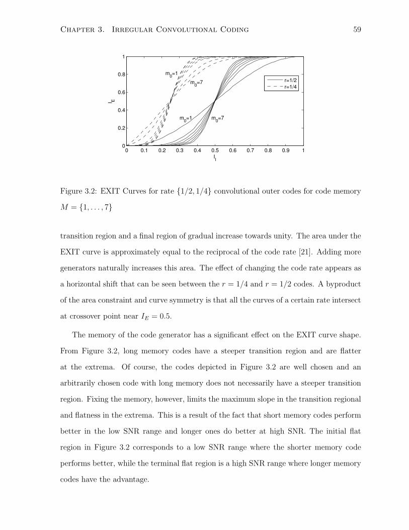
Chapter 3. Irregular Convolutional Coding 59
0 0.1 0.2 0.3 0.4 0.5 0.6 0.7 0.8 0.9 10
0.2
0.4
0.6
0.8
1
m0=1
m0=7
m0=1 m0=7
II
I E
r=1/2r=1/4
Figure 3.2: EXIT Curves for rate 1/2, 1/4 convolutional outer codes for code memory
M = 1, . . . , 7
transition region and a final region of gradual increase towards unity. The area under the
EXIT curve is approximately equal to the reciprocal of the code rate [21]. Adding more
generators naturally increases this area. The effect of changing the code rate appears as
a horizontal shift that can be seen between the r = 1/4 and r = 1/2 codes. A byproduct
of the area constraint and curve symmetry is that all the curves of a certain rate intersect
at crossover point near IE = 0.5.
The memory of the code generator has a significant effect on the EXIT curve shape.
From Figure 3.2, long memory codes have a steeper transition region and are flatter
at the extrema. Of course, the codes depicted in Figure 3.2 are well chosen and an
arbitrarily chosen code with long memory does not necessarily have a steeper transition
region. Fixing the memory, however, limits the maximum slope in the transition regional
and flatness in the extrema. This is a result of the fact that short memory codes perform
better in the low SNR range and longer ones do better at high SNR. The initial flat
region in Figure 3.2 corresponds to a low SNR range where the shorter memory code
performs better, while the terminal flat region is a high SNR range where longer memory
codes have the advantage.
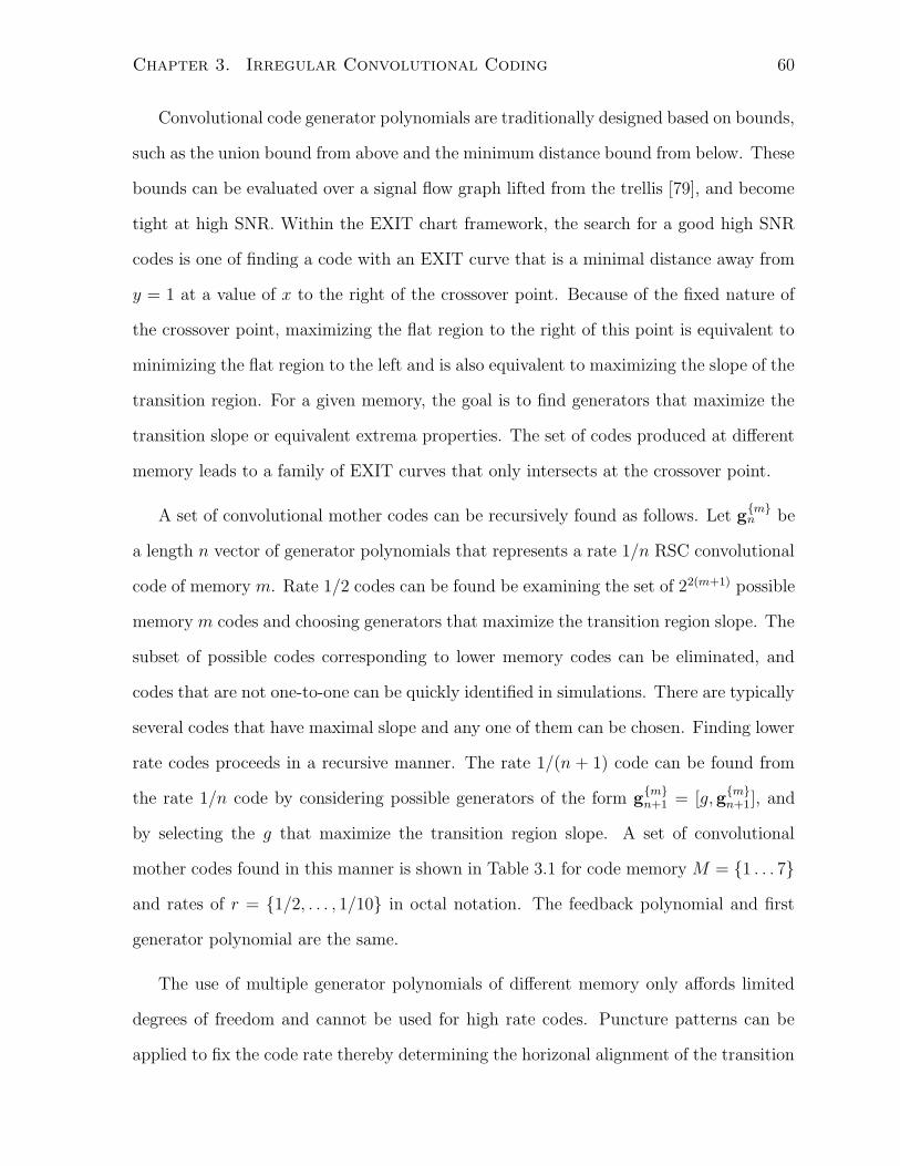
Chapter 3. Irregular Convolutional Coding 60
Convolutional code generator polynomials are traditionally designed based on bounds,
such as the union bound from above and the minimum distance bound from below. These
bounds can be evaluated over a signal flow graph lifted from the trellis [79], and become
tight at high SNR. Within the EXIT chart framework, the search for a good high SNR
codes is one of finding a code with an EXIT curve that is a minimal distance away from
y = 1 at a value of x to the right of the crossover point. Because of the fixed nature of
the crossover point, maximizing the flat region to the right of this point is equivalent to
minimizing the flat region to the left and is also equivalent to maximizing the slope of the
transition region. For a given memory, the goal is to find generators that maximize the
transition slope or equivalent extrema properties. The set of codes produced at different
memory leads to a family of EXIT curves that only intersects at the crossover point.
A set of convolutional mother codes can be recursively found as follows. Let gmn be
a length n vector of generator polynomials that represents a rate 1/n RSC convolutional
code of memory m. Rate 1/2 codes can be found be examining the set of 22(m+1) possible
memory m codes and choosing generators that maximize the transition region slope. The
subset of possible codes corresponding to lower memory codes can be eliminated, and
codes that are not one-to-one can be quickly identified in simulations. There are typically
several codes that have maximal slope and any one of them can be chosen. Finding lower
rate codes proceeds in a recursive manner. The rate 1/(n + 1) code can be found from
the rate 1/n code by considering possible generators of the form gmn+1 = [g,g
mn+1], and
by selecting the g that maximize the transition region slope. A set of convolutional
mother codes found in this manner is shown in Table 3.1 for code memory M = 1 . . . 7
and rates of r = 1/2, . . . , 1/10 in octal notation. The feedback polynomial and first
generator polynomial are the same.
The use of multiple generator polynomials of different memory only affords limited
degrees of freedom and cannot be used for high rate codes. Puncture patterns can be
applied to fix the code rate thereby determining the horizonal alignment of the transition
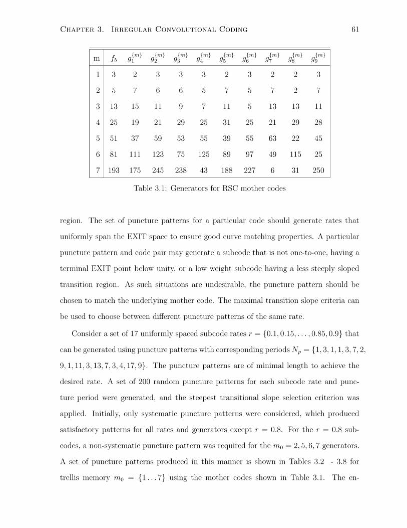
Chapter 3. Irregular Convolutional Coding 61
m fb gm1 g
m2 g
m3 g
m4 g
m5 g
m6 g
m7 g
m8 g
m9
1 3 2 3 3 3 2 3 2 2 3
2 5 7 6 6 5 7 5 7 2 7
3 13 15 11 9 7 11 5 13 13 11
4 25 19 21 29 25 31 25 21 29 28
5 51 37 59 53 55 39 55 63 22 45
6 81 111 123 75 125 89 97 49 115 25
7 193 175 245 238 43 188 227 6 31 250
Table 3.1: Generators for RSC mother codes
region. The set of puncture patterns for a particular code should generate rates that
uniformly span the EXIT space to ensure good curve matching properties. A particular
puncture pattern and code pair may generate a subcode that is not one-to-one, having a
terminal EXIT point below unity, or a low weight subcode having a less steeply sloped
transition region. As such situations are undesirable, the puncture pattern should be
chosen to match the underlying mother code. The maximal transition slope criteria can
be used to choose between different puncture patterns of the same rate.
Consider a set of 17 uniformly spaced subcode rates r = 0.1, 0.15, . . . , 0.85, 0.9 that
can be generated using puncture patterns with corresponding periods Np = 1, 3, 1, 1, 3, 7, 2,
9, 1, 11, 3, 13, 7, 3, 4, 17, 9. The puncture patterns are of minimal length to achieve the
desired rate. A set of 200 random puncture patterns for each subcode rate and punc-
ture period were generated, and the steepest transitional slope selection criterion was
applied. Initially, only systematic puncture patterns were considered, which produced
satisfactory patterns for all rates and generators except r = 0.8. For the r = 0.8 sub-
codes, a non-systematic puncture pattern was required for the m0 = 2, 5, 6, 7 generators.
A set of puncture patterns produced in this manner is shown in Tables 3.2 - 3.8 for
trellis memory m0 = 1 . . . 7 using the mother codes shown in Table 3.1. The en-

Chapter 3. Irregular Convolutional Coding 62
0.1, 1, (1, 1, 1, 1, 1, 1, 1, 1, 1, 1),0.15, 3, (7, 7, 7, 7, 7, 7, 3),0.20, 1, (1, 1, 1, 1, 1)
0.25, 1, (1, 1, 1, 1),0.30, 3, (7, 7, 7, 1),0.35, 7, (177, 177, 175)
0.40, 2, (3, 3, 1),0.45, 9, (777, 367, 245),0.50, 1, (1, 1),0.55, 11, (3777, 1577)
0.60, 3, (7, 5),0.65, 13, (17777, 10663),0.70, 7, (177, 45)
0.75, 3, (7, 1),0.80, 4, (17, 1),0.85, 17, (377777, 20101),0.90, 9, (777, 1)
Table 3.2: Puncture Patterns for m0 = 1 RSC mother codes (octal)
0.1, 1, (1, 1, 1, 1, 1, 1, 1, 1, 1, 1),0.15, 3, (7, 7, 7, 7, 7, 7, 3),0.20, 1, (1, 1, 1, 1, 1)
0.25, 1, (1, 1, 1, 1),0.30, 3, (7, 7, 7, 1),0.35, 7, (177, 177, 175)
0.40, 2, (3, 3, 1),0.45, 9, (777, 735, 454),0.50, 1, (1, 1),0.55, 11, (3777, 2776)
0.60, 3, (7, 6),0.65, 13, (17777, 11631),0.70, 7, (177, 107)
0.75, 3, (7, 1),0.80, 4, (15, 6),0.85, 17, (377777, 110040),0.90, 9, (777, 1)
Table 3.3: Puncture Patterns for m0 = 2 RSC mother codes (octal)
try r,Np, (p1, p2, . . . , pnr)) has rate r, puncture period Np with a puncture pattern
(p1, p2, . . . , pnr) specified in octal notation. For example, the rate 0.45 entry for the
m0 = 1 code generators in Table 3.2 has a puncture period of 9 and a puncture pat-
tern of (777, 367, 245) in octal or (111111111, 011110111, 010100101) in binary. This is a
systematic puncture pattern since none of the first generator bits are punctured.
The set of EXIT curves produced from the generators in Table 3.1 and puncture
patterns from Tables 3.2 - 3.8 are shown in Figure 3.3. For a given memory, the set of rate
compatible EXIT curves do not intersect. For a particular rate, codes of different memory
only intersect at the terminal points and a crossover point near IE = 0.5, decreasing
slightly for high rate codes.
The overall irregular convolutional code is constructed by encoding different fractions
of bits with different mother codes, and by puncturing with the appropriate patterns.
Let λm,p be the fraction of coded bits produced by the memory m mother encoder and

Chapter 3. Irregular Convolutional Coding 63
0.1, 1, (1, 1, 1, 1, 1, 1, 1, 1, 1, 1),0.15, 3, (7, 7, 7, 7, 7, 7, 3),0.20, 1, (1, 1, 1, 1, 1)
0.25, 1, (1, 1, 1, 1),0.30, 3, (7, 7, 7, 1),0.35, 7, (177, 157, 177)
0.40, 2, (3, 3, 1),0.45, 9, (777, 171, 746),0.50, 1, (1, 1),0.55, 11, (3777, 1767)
0.60, 3, (7, 6),0.65, 13, (17777, 6554),0.70, 7, (177, 26)
0.75, 3, (7, 1),0.80, 4, (17, 1),0.85, 17, (377777, 4060),0.90, 9, (777, 1)
Table 3.4: Puncture Patterns for m0 = 3 RSC mother codes (octal)
0.1, 1, (1, 1, 1, 1, 1, 1, 1, 1, 1, 1),0.15, 3, (7, 7, 7, 7, 7, 7, 3),0.20, 1, (1, 1, 1, 1, 1)
0.25, 1, (1, 1, 1, 1),0.30, 3, (7, 7, 7, 1),0.35, 7, (177, 77, 175)
0.40, 2, (3, 3, 1),0.45, 9, (777, 176, 661),0.50, 1, (1, 1),0.55, 11, (3777, 3567)
0.60, 3, (7, 3),0.65, 13, (17777, 1553),0.70, 7, (177, 64)
0.75, 3, (7, 1),0.80, 4, (17, 1),0.85, 17, (377777, 220004),0.90, 9, (777, 1)
Table 3.5: Puncture Patterns for m0 = 4 RSC mother codes (octal)
0.1, 1, (1, 1, 1, 1, 1, 1, 1, 1, 1, 1),0.15, 3, (7, 7, 7, 7, 7, 7, 3),0.20, 1, (1, 1, 1, 1, 1)
0.25, 1, (1, 1, 1, 1),0.30, 3, (7, 7, 7, 1),0.35, 7, (177, 167, 175)
0.40, 2, (3, 3, 1),0.45, 9, (777, 643, 535),0.50, 1, (1, 1),0.55, 11, (3777, 3753)
0.60, 3, (7, 5),0.65, 13, (17777, 5037),0.70, 7, (177, 45)
0.75, 3, (7, 1),0.80, 4, (10, 17),0.85, 17, (377777, 2420),0.90, 9, (777, 1)
Table 3.6: Puncture Patterns for m0 = 5 RSC mother codes (octal)
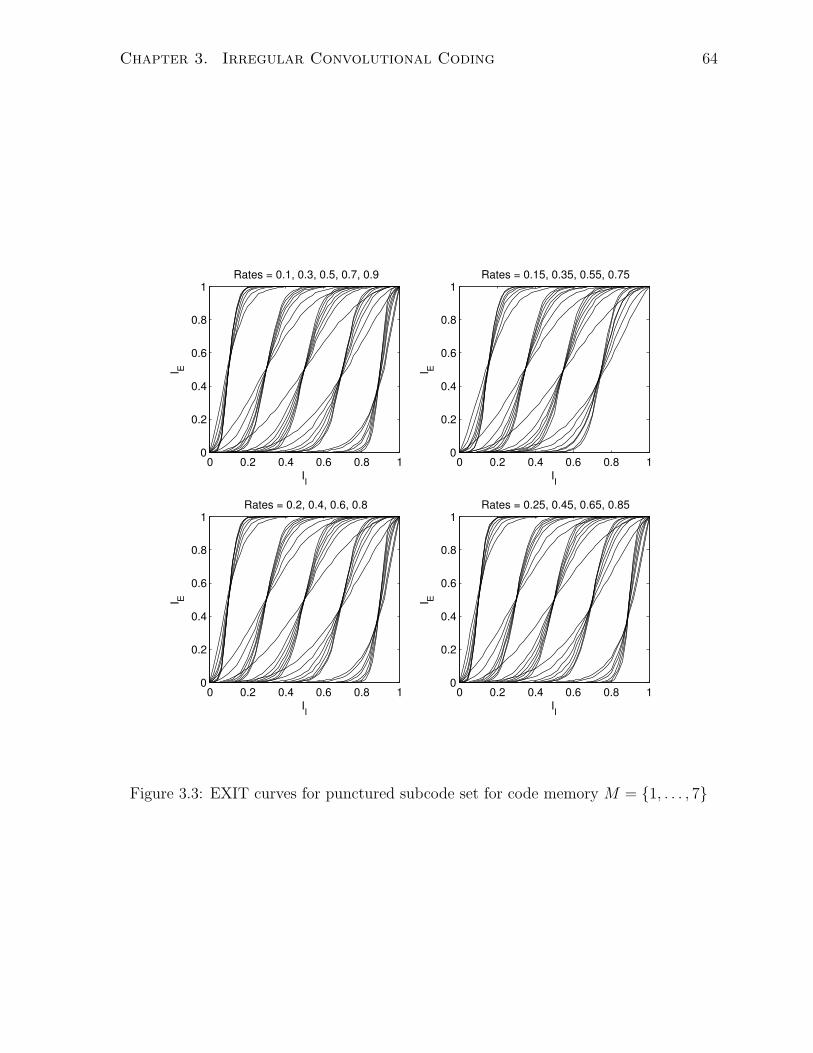
Chapter 3. Irregular Convolutional Coding 64
0 0.2 0.4 0.6 0.8 10
0.2
0.4
0.6
0.8
1Rates = 0.1, 0.3, 0.5, 0.7, 0.9
II
I E
0 0.2 0.4 0.6 0.8 10
0.2
0.4
0.6
0.8
1Rates = 0.15, 0.35, 0.55, 0.75
II
I E
0 0.2 0.4 0.6 0.8 10
0.2
0.4
0.6
0.8
1Rates = 0.2, 0.4, 0.6, 0.8
II
I E
0 0.2 0.4 0.6 0.8 10
0.2
0.4
0.6
0.8
1Rates = 0.25, 0.45, 0.65, 0.85
II
I E
Figure 3.3: EXIT curves for punctured subcode set for code memory M = 1, . . . , 7

Chapter 3. Irregular Convolutional Coding 65
0.1, 1, (1, 1, 1, 1, 1, 1, 1, 1, 1, 1),0.15, 3, (7, 7, 7, 7, 7, 7, 3),0.20, 1, (1, 1, 1, 1, 1)
0.25, 1, (1, 1, 1, 1),0.30, 3, (7, 7, 7, 1),0.35, 7, (177, 137, 177)
0.40, 2, (3, 2, 3),0.45, 9, (777, 771, 452),0.50, 1, (1, 1),0.55, 11, (3777, 1776)
0.60, 3, (7, 1),0.65, 13, (17777, 15644),0.70, 7, (177, 31)
0.75, 3, (7, 1),0.80, 4, (14, 7),0.85, 17, (377777, 124000),0.90, 9, (777, 1)
Table 3.7: Puncture Patterns for m0 = 6 RSC mother codes (octal)
0.1, 1, (1, 1, 1, 1, 1, 1, 1, 1, 1, 1),0.15, 3, (7, 7, 7, 7, 7, 7, 3),0.20, 1, (1, 1, 1, 1, 1)
0.25, 1, (1, 1, 1, 1),0.30, 3, (7, 7, 7, 1),0.35, 7, (177, 157, 177)
0.40, 2, (3, 3, 1),0.45, 9, (777, 637, 113),0.50, 1, (1, 1),0.55, 11, (3777, 3537)
0.60, 3, (7, 6),0.65, 13, (17777, 6552),0.70, 7, (177, 46)
0.75, 3, (7, 1),0.80, 4, (17, 1),0.85, 17, (377777, 202200),0.90, 9, (777, 1)
Table 3.8: Puncture Patterns for m0 = 7 RSC mother codes (octal)
punctured with the corresponding pth puncture pattern in the mth subset. It is convenient
to index over m and p using a single variable i = m ∗P + p, where P = 17 is the number
of puncture patterns per code. The optimal degree distribution λi∗ can be found as
the solution to the following constrained rate maximization problem:
arg maxλi
Pmmax0∑
i=1
λiri s.t.∑
λi = 1,∑
λific (II) > f−1
ch (II)∀II (3.5)
where ri is the rate of the ith subcode, fic (II) is the ith subcode EXIT curve, and f−1
ch (II)
is the inverse channel EXIT function. The problem in (3.5) can be solved using a gradient
search technique discussed in Chapter 2, with additional upper bound constraints to aid
in convergence.
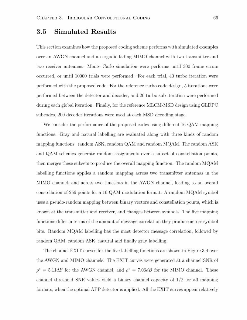
Chapter 3. Irregular Convolutional Coding 66
3.5 Simulated Results
This section examines how the proposed coding scheme performs with simulated examples
over an AWGN channel and an ergodic fading MIMO channel with two transmitter and
two receiver antennas. Monte Carlo simulation were performs until 300 frame errors
occurred, or until 10000 trials were performed. For each trial, 40 turbo iteration were
performed with the proposed code. For the reference turbo code design, 5 iterations were
performed between the detector and decoder, and 20 turbo sub-iteration were performed
during each global iteration. Finally, for the reference MLCM-MSD design using GLDPC
subcodes, 200 decoder iterations were used at each MSD decoding stage.
We consider the performance of the proposed codes using different 16-QAM mapping
functions. Gray and natural labelling are evaluated along with three kinds of random
mapping functions: random ASK, random QAM and random MQAM. The random ASK
and QAM schemes generate random assignments over a subset of constellation points,
then merges these subsets to produce the overall mapping function. The random MQAM
labelling functions applies a random mapping across two transmitter antennas in the
MIMO channel, and across two timeslots in the AWGN channel, leading to an overall
constellation of 256 points for a 16-QAM modulation format. A random MQAM symbol
uses a pseudo-random mapping between binary vectors and constellation points, which is
known at the transmitter and receiver, and changes between symbols. The five mapping
functions differ in terms of the amount of message correlation they produce across symbol
bits. Random MQAM labelling has the most detector message correlation, followed by
random QAM, random ASK, natural and finally gray labelling.
The channel EXIT curves for the five labelling functions are shown in Figure 3.4 over
the AWGN and MIMO channels. The EXIT curves were generated at a channel SNR of
ρ∗ = 5.11dB for the AWGN channel, and ρ∗ = 7.06dB for the MIMO channel. These
channel threshold SNR values yield a binary channel capacity of 1/2 for all mapping
formats, when the optimal APP detector is applied. All the EXIT curves appear relatively

Chapter 3. Irregular Convolutional Coding 67
0 0.5 10
0.1
0.2
0.3
0.4
0.5
0.6
0.7
0.8
0.9
1AWGN
II
I E
0 0.5 10
0.1
0.2
0.3
0.4
0.5
0.6
0.7
0.8
0.9
12x2 Rayleigh
III E
GrayNaturalRand ASKRand QAMRand MQAMErr Floor Mod
Figure 3.4: Channel EXIT curves for different 16-QAM mapping functions over the
AWGN and 2× 2 MIMO fading channel.
straight, with a slope that is strongly influenced by the mapping function. Gray labelling
produces a nearly horizontal curve followed by natural labelling, random ASK, random
QAM, and random MQAM labelling. The MIMO channel EXIT curves are consistently
steeper than the corresponding AWGN channel curves. Also shown in Figure 3.4 is a
modified channel EXIT curve for all the mapping functions except the random MQAM.
The modified channel curves are produced by reducing the terminal EXIT point according
to fch(1) ← max(0.95fch(1), fch(0.9)), and interpolating. This modification can lead to
improved error floor performance for some mapping functions.
Using the code optimization in (3.5), irregular code profiles were generated at different
SNR values until a rate 1/2 code was produced. The set of code threshold SNR’s that
yielding rate 1/2 codes is shown in Table 3.9, for a maximum convolution code memory
of M = 4, 7. For both the AWGN and MIMO channels, steeper channel EXIT curves
lead to lower code threshold values. The EXIT chart predicted code threshold for the
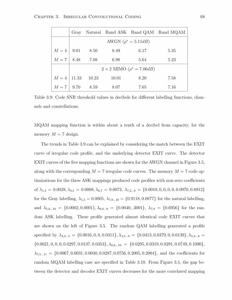
Chapter 3. Irregular Convolutional Coding 68
Gray Natural Rand ASK Rand QAM Rand MQAM
AWGN (ρ∗ = 5.11dB)
M = 4 9.01 8.50 8.49 6.17 5.35
M = 7 8.48 7.08 6.98 5.64 5.23
2× 2 MIMO (ρ∗ = 7.06dB)
M = 4 11.33 10.23 10.01 8.20 7.58
M = 7 9.70 8.59 8.07 7.65 7.16
Table 3.9: Code SNR threshold values in decibels for different labelling functions, chan-
nels and constellations.
MQAM mapping function is within about a tenth of a decibel from capacity, for the
memory M = 7 design.
The trends in Table 3.9 can be explained by considering the match between the EXIT
curve of irregular code profile, and the underlying detector EXIT curve. The detector
EXIT curves of the five mapping functions are shown for the AWGN channel in Figure 3.5,
along with the corresponding M = 7 irregular code curves. The memory M = 7 code op-
timizations for the three ASK mappings produced code profiles with non-zero coefficients
of λ1,3 = 0.0028, λ3,5 = 0.0008, λ6,7 = 0.0073, λ7,2...8 = 0.0010, 0, 0, 0, 0, 0.0970, 0.8912
for the Gray labelling, λ1,5 = 0.0005, λ7,9...10 = 0.9118, 0.0877 for the natural labelling,
and λ5,9...10 = 0.0002, 0.0001, λ6,8...9 = 0.0040, .3001, λ7,9 = 0.6956 for the ran-
dom ASK labelling. These profile generated almost identical code EXIT curves that
are shown on the left of Figure 3.5. The random QAM labelling generated a profile
specified by λ3,3...5 = 0.0016, 0, 0, 0.0311, λ4,5...9 = 0.0413, 0.0379, 0, 0.0139, λ5,2...8 =
0.0021, 0, 0, 0, 0.0297, 0.0137, 0.0353, λ6,6...10 = 0.0295, 0.0319, 0.0291, 0.0749, 0.1090,
λ7,5...11 = 0.0067, 0.0031, 0.0040, 0.0287, 0.0756, 0.2005, 0.2004, and the coefficients for
random MQAM labelling case are specified in Table 3.10. From Figure 3.5, the gap be-
tween the detector and decoder EXIT curves decreases for the more correlated mapping
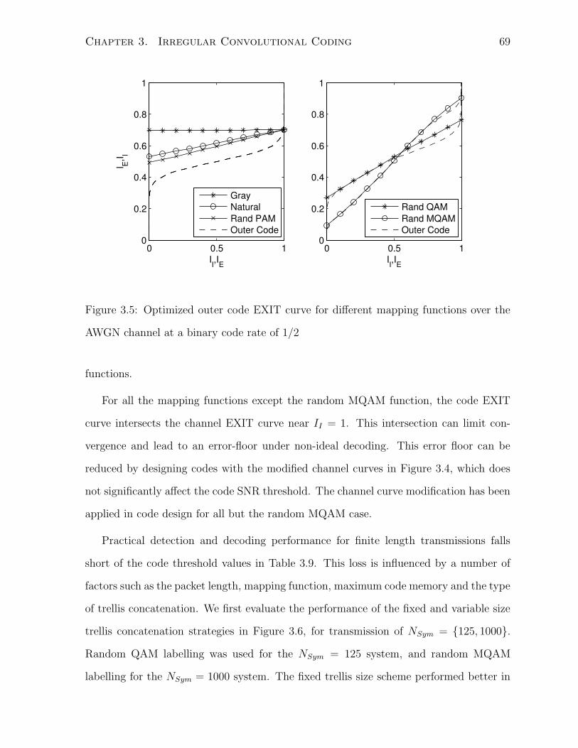
Chapter 3. Irregular Convolutional Coding 69
0 0.5 10
0.2
0.4
0.6
0.8
1
II,IE
I E,I I
0 0.5 10
0.2
0.4
0.6
0.8
1
II,IE
GrayNaturalRand PAMOuter Code
Rand QAMRand MQAMOuter Code
Figure 3.5: Optimized outer code EXIT curve for different mapping functions over the
AWGN channel at a binary code rate of 1/2
functions.
For all the mapping functions except the random MQAM function, the code EXIT
curve intersects the channel EXIT curve near II = 1. This intersection can limit con-
vergence and lead to an error-floor under non-ideal decoding. This error floor can be
reduced by designing codes with the modified channel curves in Figure 3.4, which does
not significantly affect the code SNR threshold. The channel curve modification has been
applied in code design for all but the random MQAM case.
Practical detection and decoding performance for finite length transmissions falls
short of the code threshold values in Table 3.9. This loss is influenced by a number of
factors such as the packet length, mapping function, maximum code memory and the type
of trellis concatenation. We first evaluate the performance of the fixed and variable size
trellis concatenation strategies in Figure 3.6, for transmission of NSym = 125, 1000.
Random QAM labelling was used for the NSym = 125 system, and random MQAM
labelling for the NSym = 1000 system. The fixed trellis size scheme performed better in
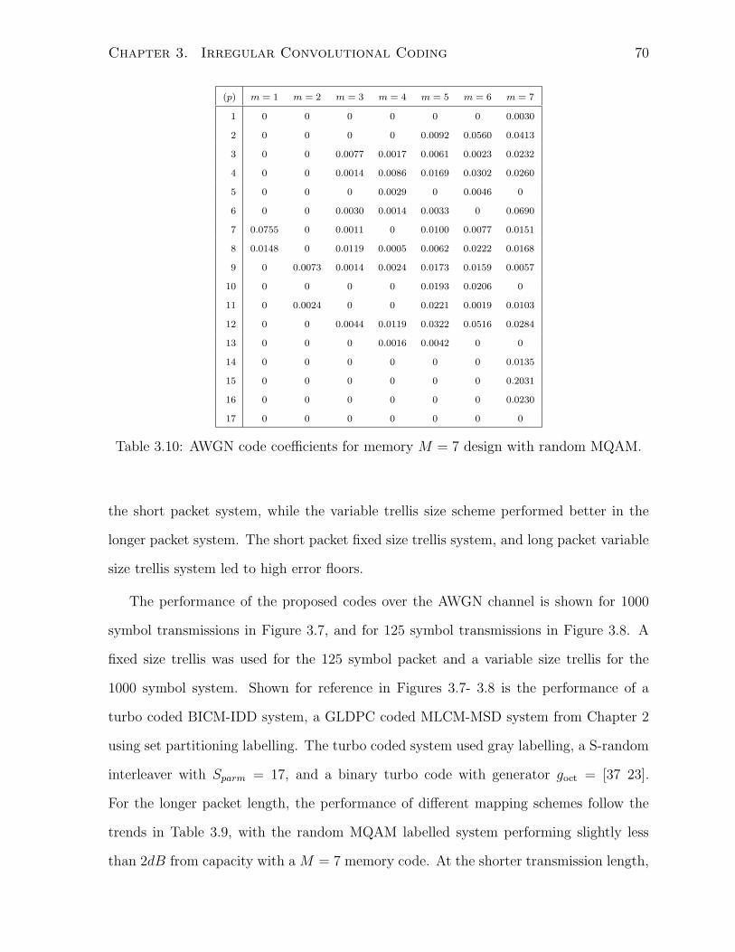
Chapter 3. Irregular Convolutional Coding 70
(p) m = 1 m = 2 m = 3 m = 4 m = 5 m = 6 m = 7
1 0 0 0 0 0 0 0.0030
2 0 0 0 0 0.0092 0.0560 0.0413
3 0 0 0.0077 0.0017 0.0061 0.0023 0.0232
4 0 0 0.0014 0.0086 0.0169 0.0302 0.0260
5 0 0 0 0.0029 0 0.0046 0
6 0 0 0.0030 0.0014 0.0033 0 0.0690
7 0.0755 0 0.0011 0 0.0100 0.0077 0.0151
8 0.0148 0 0.0119 0.0005 0.0062 0.0222 0.0168
9 0 0.0073 0.0014 0.0024 0.0173 0.0159 0.0057
10 0 0 0 0 0.0193 0.0206 0
11 0 0.0024 0 0 0.0221 0.0019 0.0103
12 0 0 0.0044 0.0119 0.0322 0.0516 0.0284
13 0 0 0 0.0016 0.0042 0 0
14 0 0 0 0 0 0 0.0135
15 0 0 0 0 0 0 0.2031
16 0 0 0 0 0 0 0.0230
17 0 0 0 0 0 0 0
Table 3.10: AWGN code coefficients for memory M = 7 design with random MQAM.
the short packet system, while the variable trellis size scheme performed better in the
longer packet system. The short packet fixed size trellis system, and long packet variable
size trellis system led to high error floors.
The performance of the proposed codes over the AWGN channel is shown for 1000
symbol transmissions in Figure 3.7, and for 125 symbol transmissions in Figure 3.8. A
fixed size trellis was used for the 125 symbol packet and a variable size trellis for the
1000 symbol system. Shown for reference in Figures 3.7- 3.8 is the performance of a
turbo coded BICM-IDD system, a GLDPC coded MLCM-MSD system from Chapter 2
using set partitioning labelling. The turbo coded system used gray labelling, a S-random
interleaver with Sparm = 17, and a binary turbo code with generator goct = [37 23].
For the longer packet length, the performance of different mapping schemes follow the
trends in Table 3.9, with the random MQAM labelled system performing slightly less
than 2dB from capacity with a M = 7 memory code. At the shorter transmission length,

Chapter 3. Irregular Convolutional Coding 71
4 4.5 5 5.5 6 6.5 7 7.5 8 8.5 910−4
10−3
10−2
10−1
100
FER
Es/N0(dB)
Ns=125, Fixed Size
Ns=125, Var Size
Ns=1000, Fixed Size
Ns=1000, Var Size
Figure 3.6: FER performance of 16-QAM BICM system over AWGN channel using fixed
and variable sized trellises.
the performance of the random MQAM scheme is limited by high detector message
correlation, and the random ASK and random QAM designs perform better. For the
random QAM mapping, there is minimal loss is using a less complex memory M = 4
code at frame error rates above FER = 0.005. In comparison to the reference designs,
however, the proposed codes do not perform as well as either the turbo coded system or
the GLDPC coded MLCM-MSD system.
The performance of the proposed codes over the 2 × 2 MIMO channel is shown in
Figure 3.9 for 1000 symbol blocks and in Figure 3.10 for 125 symbol blocks. The perfor-
mance trends across mapping functions and packet lengths generally follow the AWGN
channel trends. Performance within 2dB − 2.5dB of capacity is possible with M = 7
designs using random QAM and random MQAM labelling for 1000 symbol packets, and
random ASK and natural labelling for 125 symbol packets. At both packet lengths, the
random MQAM labelled M = 4 design outperforms both the reference turbo coded sys-

Chapter 3. Irregular Convolutional Coding 72
5 5.5 6 6.5 7 7.5 8
10−3
10−2
10−1
100
FER
Es/N0(dB)
m0=7
m0=4
Rnd PAMRnd QAMRnd MQAMTurbo CodeMLCM GLDPC
Figure 3.7: AWGN channel performance of proposed codes for 2000 symbol transmissions.
5 5.5 6 6.5 7 7.5 8 8.5 910−4
10−3
10−2
10−1
100
FER
Es/N0(dB)
m0=7
m0=4
Rnd PAMRnd QAMRnd MQAMTurbo CodeMLCM GLDPC
Figure 3.8: AWGN channel performance of proposed codes for 250 symbol transmissions.
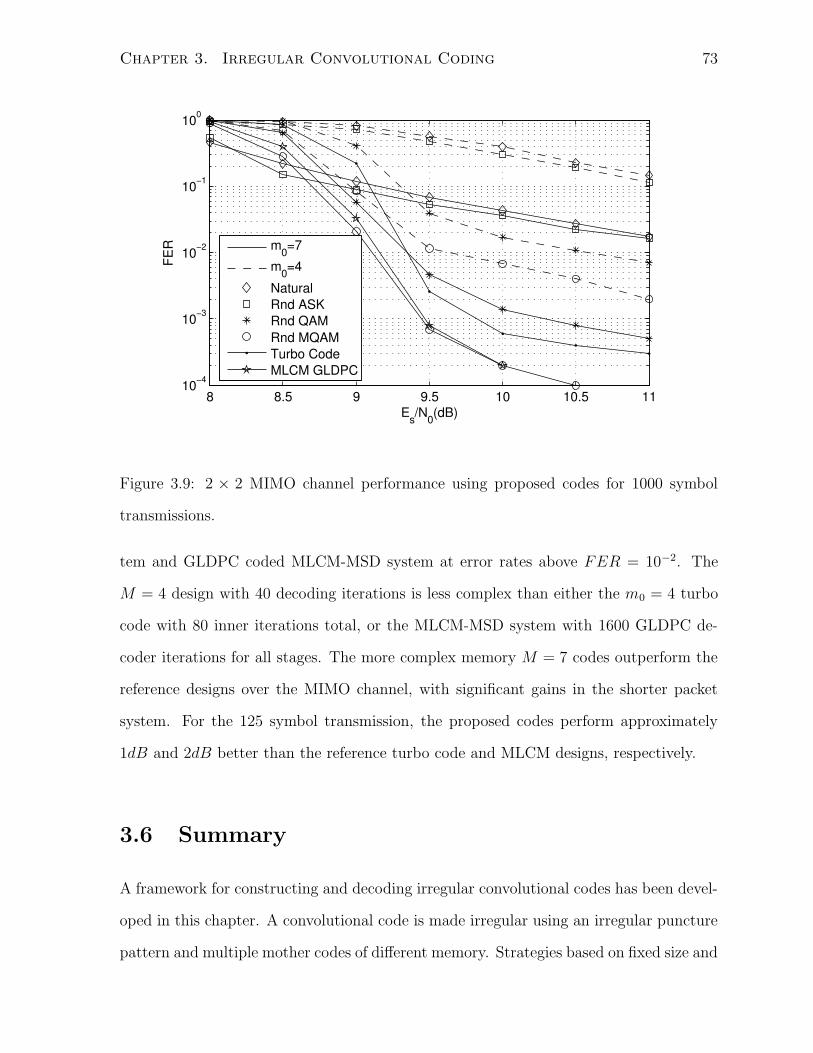
Chapter 3. Irregular Convolutional Coding 73
8 8.5 9 9.5 10 10.5 1110−4
10−3
10−2
10−1
100
FER
Es/N0(dB)
m0=7
m0=4
NaturalRnd ASKRnd QAMRnd MQAMTurbo CodeMLCM GLDPC
Figure 3.9: 2 × 2 MIMO channel performance using proposed codes for 1000 symbol
transmissions.
tem and GLDPC coded MLCM-MSD system at error rates above FER = 10−2. The
M = 4 design with 40 decoding iterations is less complex than either the m0 = 4 turbo
code with 80 inner iterations total, or the MLCM-MSD system with 1600 GLDPC de-
coder iterations for all stages. The more complex memory M = 7 codes outperform the
reference designs over the MIMO channel, with significant gains in the shorter packet
system. For the 125 symbol transmission, the proposed codes perform approximately
1dB and 2dB better than the reference turbo code and MLCM designs, respectively.
3.6 Summary
A framework for constructing and decoding irregular convolutional codes has been devel-
oped in this chapter. A convolutional code is made irregular using an irregular puncture
pattern and multiple mother codes of different memory. Strategies based on fixed size and
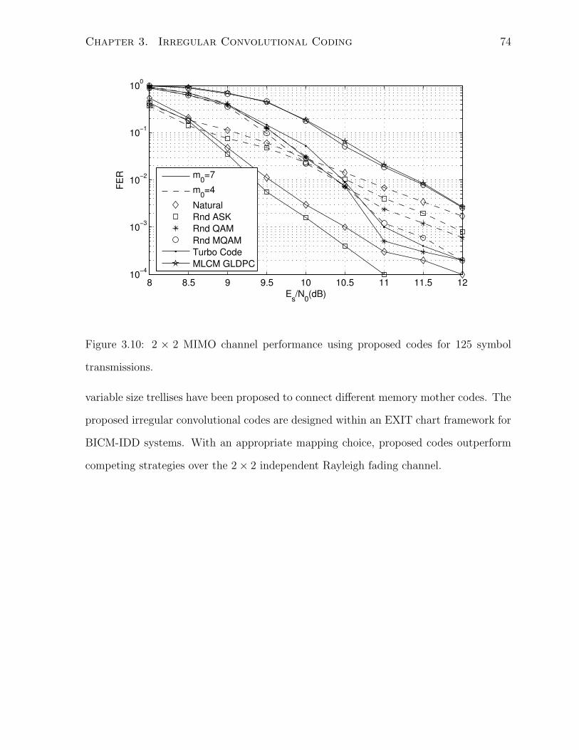
Chapter 3. Irregular Convolutional Coding 74
8 8.5 9 9.5 10 10.5 11 11.5 1210−4
10−3
10−2
10−1
100
FER
Es/N0(dB)
m0=7
m0=4
NaturalRnd ASKRnd QAMRnd MQAMTurbo CodeMLCM GLDPC
Figure 3.10: 2 × 2 MIMO channel performance using proposed codes for 125 symbol
transmissions.
variable size trellises have been proposed to connect different memory mother codes. The
proposed irregular convolutional codes are designed within an EXIT chart framework for
BICM-IDD systems. With an appropriate mapping choice, proposed codes outperform
competing strategies over the 2× 2 independent Rayleigh fading channel.
Chapter 4
Iterative Space-Time Detection
This chapter steps back from the coded modulation designs proposed in the previous two
chapters and looks at receiver processing. In large systems, optimal detection becomes
impractical so less complex designs must be employed. Two novel detectors are developed
in this chapter based on a group strategy that can be used in an IDD receiver. As the
focus in this chapter is receiver processing, simple convolutional outer-codes are used
in a D-BLAST space-time architecture. The work in this is chapter has largely been
published in [96, 97, 98].
4.1 Introduction
The use of multiple transmitter and receiver antennas can provide tremendous capacity
increases in wireless fading environments [1]. The BLAST architecture [9] is a simple
and efficient multiplexing structure that can take advantage of the multi-antenna channel
capacity. It is often decoded using an MSD receiver with linear detector processing, and
is effective in systems having an excess number of transmitter antennas [99].
There are several detection strategies that can be applied to systems having an ex-
cess number of transmitter antennas. An optimal solution is the ML detector. The ML
detector unfortunately has exponential complexity that grows with Rn, where R is the
75

Chapter 4. Iterative Space-Time Detection 76
constellation size and n is the number of transmitter antennas. The ML detector can be
implemented using the sphere decoding algorithm [100] with some complexity savings.
Sphere decoding still has exponential worst-case complexity, although the average-case
complexity can be polynomial at high SNR [101]. Suboptimal ML detectors have been ap-
plied to BLAST systems using tree-search algorithms [102] and group detection strategies
[103, 104]. Group detection has also been extensively used in the context of multi-user
detection [105, 106, 107, 108, 109, 110].
Iterative detection and decoding is an effective way to improve the performance of a
BLAST receiver. Layered IDD receivers have been employed in [111, 112, 113], which
consist of an iterative exchange of soft information between the detector and the decoders.
The optimal soft-input soft-output (SISO) detector is the maximum a posteriori (MAP)
detector, which, like the ML detector, has an exponential complexity that grows with Rn.
For systems with a large number of transmitter antennas, a computationally more feasible
minimum mean squared error (MMSE) detector has been proposed, first in the multiuser
context [114, 115] and later applied to BLAST [116, 117]. The detector discussed in
[116, 117] uses soft interference cancellation with an instantaneous MMSE filter that
only suppresses residual interference that has not been cancelled. The performance of
the SISO MMSE detector improves dramatically with successive iterations, but falls
short of the MAP detector performance especially in systems having a significant excess
number of transmitter antennas.
In this chapter, two novel detectors are proposed termed the Reduced Dimension
MAP (RDMAP) detector and Group MAP (GMAP) detector, which are both based on
a group detection strategy. These detectors bridge the performance gap between MAP
and MMSE detectors in systems with an excess number of transmitter antennas and
are developed for Quadrature Amplitude Modulation (QAM). The RDMAP and GMAP
detectors operate by dividing the symbol vector into two groups: a MAP group and an
interfering group. In the RDMAP detector, the MAP and interfering groups are formed
Chapter 4. Iterative Space-Time Detection 77
dynamically for each bit decision. The GMAP detector reduces the complexity of the
RDMAP detector by using a static set of disjoint MAP groups and jointly produces a bit
decision for each bit in the group. A novel greedy algorithm is proposed to form the MAP
groups for the GMAP detector. For both detectors, the symbols in the interfering group
are treated as an interfering noise source that is whitened by applying an appropriate
filter. The prior probabilities for the interfering symbols are used to determine the mean
of the interfering noise source. The size of the MAP group NG is an adjustable parameter
that determines the detector complexity. Through the choice of this parameter, the
RDMAP and GMAP detectors are generalizations of both the MAP detector and the
MMSE detector in [116, 117].
An uncoded BER analysis of the RDMAP and GMAP detectors is also presented
in this chapter for a quasi-static Rayleigh fading channel. By approximating the MAP
decision rule with the ML decision rule, the union bound on the symbol error rate prob-
ability can be expressed as the sum of Hermitian quadratic forms in complex Gaussian
variables. The BER is obtained from the pdf of summed Hermitian quadratic forms.
4.2 System Model
4.2.1 Layered Space-Time Transmitter
Consider the transmitter structure in Figure 4.1 for a layered space-time architecture [116]
having N transmitter antennas. Binary data is demultiplexed into 2NQ bit streams that
are independently encoded and interleaved. An QAM symbol is generated by a group of
Q bit streams using a Gray labelling scheme. The nth modulated output or layer is given
by xn(k) = Mary(b(n−1)Q+1(2k) . . . bnQ(2k))+√−1Mary(b(n−1)Q+1(2k+1) . . . bnQ(2k+1)),
where Mary is the Gray coded M-ary modulating function whose output is −2Q−1 −
1,−2Q−1 + 3, . . . , 2Q−1 + 1. For QPSK, the nth layer modulated output is given by
xn(k) = 2bn(2k)− 1+√−12bn(2k + 1)− 1. The modulated output from each layer
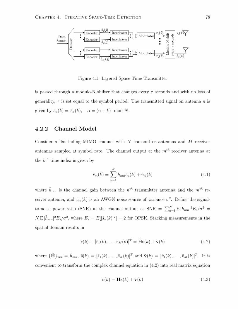
Chapter 4. Iterative Space-Time Detection 78
Modulo
-N s
hift
ever
yse
conds
t
Dem
ux
Encoder Interleaverb j1( )
DataSource Encoder
Modulator
Encoder
EncoderModulator
Interleaver
Interleaver
Interleaver
b jQ( )
b jNQ( )
~x k1( )
~x kN( )
~s k1( )
~s kN( )
Figure 4.1: Layered Space-Time Transmitter
is passed through a modulo-N shifter that changes every τ seconds and with no loss of
generality, τ is set equal to the symbol period. The transmitted signal on antenna n is
given by sn(k) = xα(k), α = (n− k) mod N .
4.2.2 Channel Model
Consider a flat fading MIMO channel with N transmitter antennas and M receiver
antennas sampled at symbol rate. The channel output at the mth receiver antenna at
the kth time index is given by
rm(k) =N∑
n=1
hmnsn(k) + vm(k) (4.1)
where hmn is the channel gain between the nth transmitter antenna and the mth re-
ceiver antenna, and vm(k) is an AWGN noise source of variance σ2. Define the signal-
to-noise power ratio (SNR) at the channel output as SNR =∑N
n=1 E |hmn|2Es/σ2 =
N E |hmn|2Es/σ2, where Es = E[|sn(k)|2] = 2 for QPSK. Stacking measurements in the
spatial domain results in
r(k) ≡ [r1(k), . . . , rM(k)]T = Hs(k) + v(k) (4.2)
where Hmn = hmn, s(k) = [s1(k), . . . , sN(k)]T and v(k) = [v1(k), . . . , vM(k)]T . It is
convenient to transform the complex channel equation in (4.2) into real matrix equation
r(k) = Hs(k) + v(k) (4.3)
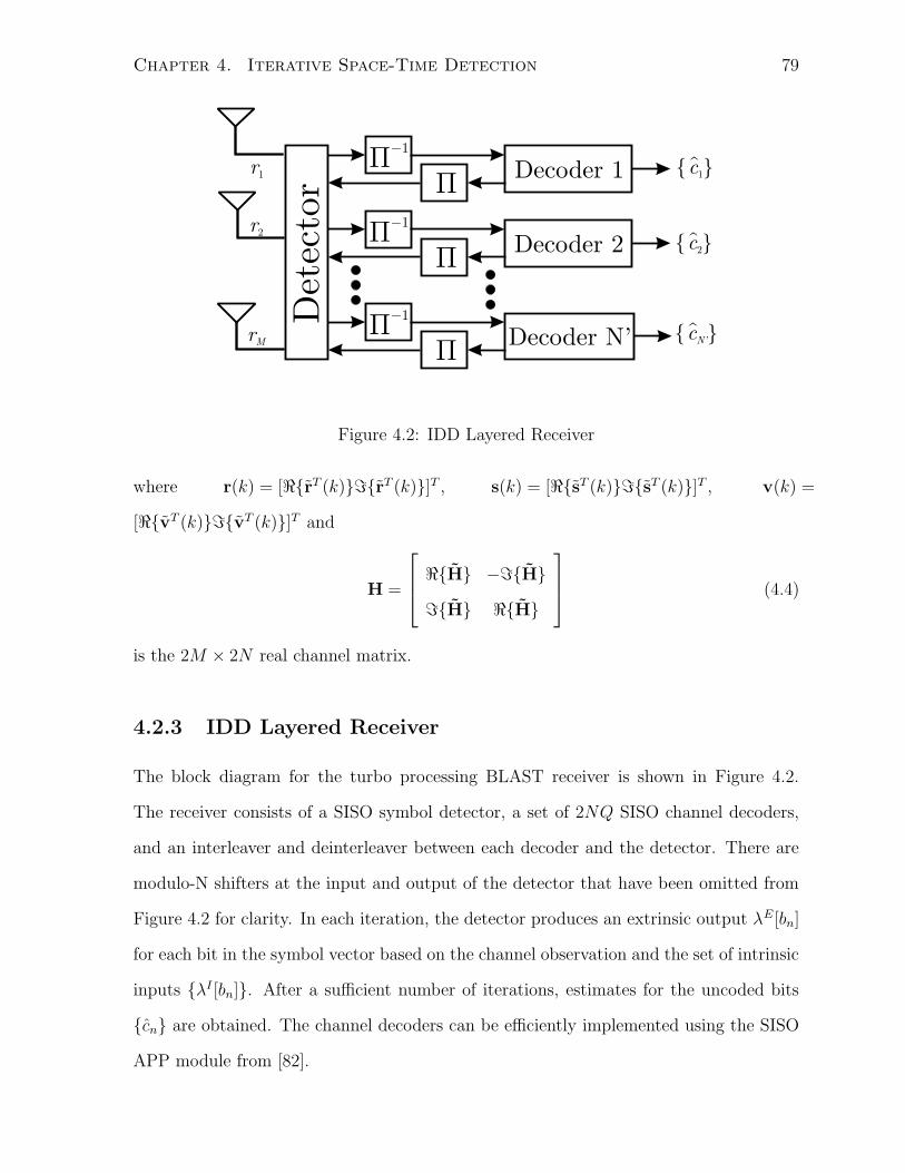
Chapter 4. Iterative Space-Time Detection 79
r1
r2
rM
^c1
^c2
^ cN’
Det
ecto
r
P-1
PDecoder 1
P-1
P
P-1
P
Decoder 2
Decoder N’
Figure 4.2: IDD Layered Receiver
where r(k) = [<rT (k)=rT (k)]T , s(k) = [<sT (k)=sT (k)]T , v(k) =
[<vT (k)=vT (k)]T and
H =
<H −=H
=H <H
(4.4)
is the 2M × 2N real channel matrix.
4.2.3 IDD Layered Receiver
The block diagram for the turbo processing BLAST receiver is shown in Figure 4.2.
The receiver consists of a SISO symbol detector, a set of 2NQ SISO channel decoders,
and an interleaver and deinterleaver between each decoder and the detector. There are
modulo-N shifters at the input and output of the detector that have been omitted from
Figure 4.2 for clarity. In each iteration, the detector produces an extrinsic output λE[bn]
for each bit in the symbol vector based on the channel observation and the set of intrinsic
inputs λI [bn]. After a sufficient number of iterations, estimates for the uncoded bits
cn are obtained. The channel decoders can be efficiently implemented using the SISO
APP module from [82].
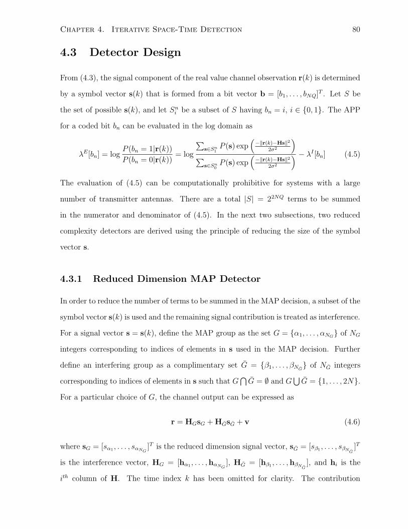
Chapter 4. Iterative Space-Time Detection 80
4.3 Detector Design
From (4.3), the signal component of the real value channel observation r(k) is determined
by a symbol vector s(k) that is formed from a bit vector b = [b1, . . . , bNQ]T . Let S be
the set of possible s(k), and let Sni be a subset of S having bn = i, i ∈ 0, 1. The APP
for a coded bit bn can be evaluated in the log domain as
λE[bn] = logP (bn = 1|r(k))
P (bn = 0|r(k))= log
∑
s∈Sn1
P (s) exp(
−‖r(k)−Hs‖2
2σ2
)
∑
s∈Sn0
P (s) exp(
−‖r(k)−Hs‖2
2σ2
) − λI [bn] (4.5)
The evaluation of (4.5) can be computationally prohibitive for systems with a large
number of transmitter antennas. There are a total |S| = 22NQ terms to be summed
in the numerator and denominator of (4.5). In the next two subsections, two reduced
complexity detectors are derived using the principle of reducing the size of the symbol
vector s.
4.3.1 Reduced Dimension MAP Detector
In order to reduce the number of terms to be summed in the MAP decision, a subset of the
symbol vector s(k) is used and the remaining signal contribution is treated as interference.
For a signal vector s = s(k), define the MAP group as the set G = α1, . . . , αNG of NG
integers corresponding to indices of elements in s used in the MAP decision. Further
define an interfering group as a complimentary set G = β1, . . . , βNG of NG integers
corresponding to indices of elements in s such that G⋂
G = ∅ and G⋃
G = 1, . . . , 2N.
For a particular choice of G, the channel output can be expressed as
r = HGsG + HGsG + v (4.6)
where sG = [sα1 , . . . , sαNG]T is the reduced dimension signal vector, sG = [sβ1 , . . . , sβNG
]T
is the interference vector, HG = [hα1 , . . . ,hαNG], HG = [hβ1 , . . . ,hβNG
], and hi is the
ith column of H. The time index k has been omitted for clarity. The contribution
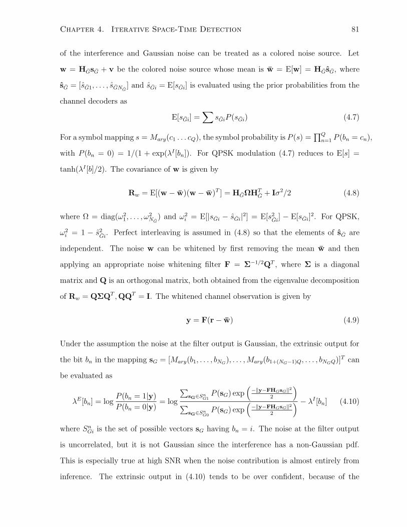
Chapter 4. Iterative Space-Time Detection 81
of the interference and Gaussian noise can be treated as a colored noise source. Let
w = HGsG + v be the colored noise source whose mean is w = E[w] = HGsG, where
sG = [sG1, . . . , sGNG] and sGi = E[sGi] is evaluated using the prior probabilities from the
channel decoders as
E[sGi] =∑
sGiP (sGi) (4.7)
For a symbol mapping s = Mary(c1 . . . cQ), the symbol probability is P (s) =∏Q
n=1 P (bn = cn),
with P (bn = 0) = 1/(1 + exp(λI [bn]). For QPSK modulation (4.7) reduces to E[s] =
tanh(λI [b]/2). The covariance of w is given by
Rw = E[(w − w)(w − w)T ] = HGΩHTG + Iσ2/2 (4.8)
where Ω = diag(ω21, . . . , ω
2NG
) and ω2i = E[|sGi − sGi|2] = E[s2
Gi] − E[sGi]
2. For QPSK,
ω2i = 1 − s2
Gi. Perfect interleaving is assumed in (4.8) so that the elements of sG are
independent. The noise w can be whitened by first removing the mean w and then
applying an appropriate noise whitening filter F = Σ−1/2QT , where Σ is a diagonal
matrix and Q is an orthogonal matrix, both obtained from the eigenvalue decomposition
of Rw = QΣQT ,QQT = I. The whitened channel observation is given by
y = F(r− w) (4.9)
Under the assumption the noise at the filter output is Gaussian, the extrinsic output for
the bit bn in the mapping sG = [Mary(b1, . . . , bNG), . . . ,Mary(b1+(NG−1)Q, . . . , bNGQ)]T can
be evaluated as
λE[bn] = logP (bn = 1|y)
P (bn = 0|y)= log
∑
sG∈SnG1
P (sG) exp(
−‖y−FHGsG‖2
2
)
∑
sG∈SnG0
P (sG) exp(
−‖y−FHGsG‖2
2
) − λI [bn] (4.10)
where SnGi is the set of possible vectors sG having bn = i. The noise at the filter output
is uncorrelated, but it is not Gaussian since the interference has a non-Gaussian pdf.
This is especially true at high SNR when the noise contribution is almost entirely from
inference. The extrinsic output in (4.10) tends to be over confident, because of the
Chapter 4. Iterative Space-Time Detection 82
assumption of Gaussian noise at the filter output. This bias can cause the IDD receiver
to diverge. In order to prevent divergence, the prior LLRs are prescaled according to
λI [b] ← sgn(λI [b])|λI [b]|κ, where 0 < κ ≤ 1. Prescaling the prior LLRs leads to an
over-estimation of the noise power from interfering symbols and compensates for the
non-Gaussian noise pdf. The prescaling function acts as a soft clipping function, whose
parameter value depends on the modulation format and will be specified in Section 4.5.
The choice of the groups G and G is critical to the performance of the RDMAP
detector. Consider forming G and G for bit decisions corresponding to a symbol si.
The biggest factor affecting the bit decision in (4.10) is the noise enhancement or signal
attenuation associated with the noise whitening filter F. The noise whitening filter
scales down the channel output in directions where the noise power is high and scales
up the channel output in directions where the noise power is low, while maintaining an
uncorrelated noise output. In order to minimize signal attenuation, the group G should
be formed such that the noise power in the direction of the signal hi is minimized. In the
channel observation space, the noise power from an interfering symbol sj, j 6= i, projected
onto the subspace of si is given by
ε2j = |hT
i hj|2ω2j (4.11)
The value of ε2j is the projected noise variance caused by sj, if it were considered in
isolation. Although the total noise power in the subspace of si is not simply the sum of
ε2j ’s, it still remains that symbols having a high ε2
j will lead to high noise enhancement
if they are placed in the interfering group. Accordingly, G is formed by the NG smallest
ε2j ’s and G is formed by the NG largest ε2
j ’s.
The MAP detector and MMSE detector in [116, 117] are special cases of the RDMAP
detector. Consider the following lemmas.
lemma 4.1: The RDMAP detector and MAP detector are equivalent for NG =
Chapter 4. Iterative Space-Time Detection 83
2N . 1
lemma 4.2: The RDMAP detector and MMSE detector in [116, 117] are equivalent
for NG = 1.
4.3.2 Group MAP Detector
The bulk of the RDMAP detector complexity lies in evaluating rG = FHGsG for all
sG ∈ SG in (4.10). The RDMAP detector uses each rG only once to produce a single bit
decision. A bit decision could be produced for all the bit used to form sG, leading to an
approximate complexity reduction of 1/NG. This is the motivation behind the GMAP
detector.
For a group G, the GMAP detector produces a log domain APP according to (4.10)
for each bit bi, i = 1 . . . NGQ corresponding to the elements of sG. With no loss of
generality, it is assumed that the symbol vector s can be divided into NΨ disjoint groups
of equal size denoted Ψ = G1, . . . , GNΨ, such that a 6= b ∀ a ∈ Gi, b ∈ Gj, i 6= j. At this
point, it can be noted that RDMAP and GMAP detectors are equivalent in the limiting
case when NG = 1 and NG = 2N . Based on lemmas 1 and 2, it can thus be concluded
that the GMAP detector is also a generalization of both the MAP detector and MMSE
detector in [116, 117].
What remains in the development of the GMAP detector is an algorithm to choose
the groups in Ψ. Like the RDMAP detector, a correlation-based grouping algorithm is
used, with a modified weighting criterion. Consider, for example, a situation in which
there is a small angle between the vectors hi and hj, but the magnitude of hj and/or ω2j
is small. The RDMAP detector would likely include si in the MAP decision group for
bj, but not include sj in the MAP decision group for bi. In a joint detection structure,
what is required is a cost metric that is symmetric to whether a decision on bi is made
with interference from sj or vice-versa. To this end, let R be the normalized correlation
1The proofs for both lemmas can be found in the Appendix A.1.
Chapter 4. Iterative Space-Time Detection 84
matrix whose entry in row i and column j is given by
rij =|hT
i hj|√
‖hi‖2‖hi‖2(4.12)
The element rij is the normalized correlation between the symbols si and sj at the channel
output. We note that if the ω2j in (4.11) were used as weights, they would be cancelled
in the normalization in (4.12).
Given a normalized correlation matrix R, consider forming Ψ using the following
objective function
Θ = arg maxG1...GNΨ
NΨ∑
k=1
arg maxj∈Gk
rij (4.13)
which is equivalent to maximizing the maximum pairwise correlation among the members
of each group, averaged over all groups. An exact solution to (4.13) requires an exhaustive
search over all possible groupings and is computationally infeasible for large N . An
approximate solution to (4.13) can be found using the following greedy algorithm
1 R← R− I;
2 Ψ← G1, . . . , G2N, Gi = i;
3 while |Ψ| > NΨ
4 if∑|Ψ|
i=1 I(|Gi| > 1) < NΨ
5 δij = I(|Gi|+ |Gj| ≤ NG);
6 else
7 δij = I(2 < |Gi|+ |Gj| ≤ NG);
8 end if
9 rkl = arg maxij rijδij;
10 Gk ← Gk ∪Gl;
11 Ψ← Ψ \ Gl;
12 for n = 1 . . . |Ψ|, n 6= k;
13 rnk = rkn = maxrnk, rnl;
Chapter 4. Iterative Space-Time Detection 85
14 end for
15 Remove kth row and column from R
16 end while
where I(x) is an indicator function that evaluates to 1 if x is true and 0 otherwise. The
preceding algorithm starts with 2N groups with one element in each and finishes with
NΨ groups with NG elements in each group. At each iteration, two groups are merged.
The list of possible groups mergers is determined in lines 4-8, and a greedy decision is
made to merge the two groups having maximum pairwise correlation. The preceding
algorithm is greedy as it attempts to form highly correlated groups first. Although this
may not optimally satisfy the objective function in (4.13), it is advantageous to form
highly correlated groups first, since the BER is more strongly influenced by groups with
a high pairwise correlation instead of by the average pairwise correlation across all groups.
4.4 BER Analysis
This section presents an analysis of the uncoded BER for the RDMAP and GMAP
detectors in a quasi-static Rayleigh fading environment. The channel coefficients hmn
are assumed to have an independent Rayleigh fading distribution with unity variance,
E[‖hmn‖2] = 1. Our analysis is based on expressing the symbol error rate as a Hermitian
quadratic form in complex Gaussian random variables, and approximating the MAP
detection rule with the ML detection rule. A similar approach has been used in the
context of multiuser detection to analyze the performance of the maximum likelihood
detector [118] and the optimal ratio combiner [119].
The RDMAP and GMAP detectors produce an a posteriori bit probability in (4.10),
with error probability Pe = P (λA[bn] < 0|bn = 1), where λA[bn] = λI [bn] + λE[bn] is
the a posteriori output. The summations in the numerator and denominator of (4.10)
are dominated by the term corresponding to the sG of closest Euclidean distance to
Chapter 4. Iterative Space-Time Detection 86
the channel observation in the noise whitened space. Approximating the summation
operators in (4.10) with max operators yields the ML decision rule, whose decision error
probability is given by
P (λA(bn) < 0|bn = 1)
≈ P
log
maxs∈Sn
G1
exp(
−‖y−FHGs‖2
2
)
maxs∈Sn
G0
exp(
−‖y−FHGs‖2
2
) < 0
(4.14)
= P
(
mins∈Sn
G1
‖y −Gs‖2 > mins∈Sn
G0
‖y −Gs‖2)
(4.15)
= P
(
s ∈ SnG0|min
s∈SnG
‖y −Gs‖2)
(4.16)
where G = FHG and SG is the set of all sG. The ML decision rule chooses the group
vector that is closest to the received vector in the noise whitened space. For a transmitted
group vector si ∈ SnG1, an erroneous decision is made if the ML detector chooses an
erroneous symbol vector sj ∈ SnG0, which will occur if Cj < Ci, where Ci is the cost
metric associated with a candidate group vector si defined by Ci , ‖y − Gsi‖2. The
probability of this pairwise error event is denoted P (Dij < 0|si), where Dij = Cj − Ci.
The union bound on the probability of a detection error for a transmitted vector
si, is given by the sum of the pairwise error probability over the set of received vectors
sj ∈ SnG0. Averaging over the set of transmitted vectors yields an upper bound of the
error probability that is given by
Pe = Esi∈Sn
G1
∑
sj∈SnG0
P (Dij < 0| si)
(4.17)
In order to evaluate (4.17), Dij can be expressed as a hermitian quadratic form in com-
plex Gaussian variables. Although it is easier to represent Dij in a real valued hermitian
quadratic form, such an expression does not allow for easy factorization, as will be dis-
cussed later. First, the group detector derived in Section 4.3 needs to be represented in
complex variables.

Chapter 4. Iterative Space-Time Detection 87
The real channel matrix consists of orthogonal pairs of column vectors hn,hn+N . Since
both the RDMAP and GMAP detectors form the MAP group G based on the correlation
between columns, it is unlikely that hn and hn+N will both be in the HG. Under this
assumption, each column in HG is orthogonal to one column in HG and approximately
independent of the remaining columns of HG,HG. The independence would be exact if
the MAP group was form by randomly choosing independent columns of H. If the set
of interfering sources sβnhβn is projected onto a column hαiof HG, there will be one
interfering source with no noise contribution and a noise contribution from the remaining
2N −NG − 1 interfering sources, each of which has a signal subspace, defined by hβn,
that is independent of hαi. If the same projection is applied to another column hαj
of
HG, there will be a different interfering source with no noise contribution and a noise
contribution from the remaining 2N −NG − 1 sources. In order to facilitate analysis, it
is assumed that there are NI = 2N − NG − 1 interfering sources whose signal subspace
is independent of HG leading an approximate channel model
r ≈ HGsG + HIsI + v (4.18)
where sI = [sI1, . . . , sINI]T is an interference vector that consists of independent elements
of unity variance, and HI is a 2M×NI Gaussian matrix that is independent of HG. Since
the grouping criterion for the RDMAP and GMAP detectors is based on the assumption
of NI independent interfering sources, one should expect the uncoded BER of both
detectors to be quite similar. Now consider the case where NI is even, letting NIc = NI/2
and impose a structure on HI of the form
HI =
HIr −HIi
HIi HIr
(4.19)
where HIr,HIi are M ×NIc matrices of independent Gaussian entries with variance 1/2.
The structure imposed in (4.19) is needed to represent the real-valued system in complex
variables. One may note that the 2N − 2NG columns of HG that are not orthogonal to
Chapter 4. Iterative Space-Time Detection 88
HG can be represented in a form similar to (4.19). Using (4.19), the real-valued channel
model in (4.18) can be equivalently represented in complex variables as
r = HGcsG + HIcsIc + v (4.20)
where HGc = HGr + iHGi such that HG = [HTGr,H
TGi]
T , HIc = HIr + iHIi and sIc =
[sI1, . . . , sINIc]T +i[sINIc+1, . . . , sINI
]T . The complex noise correlation matrix is Rwc =
HIc(2INIc)HH
Ic + IMσ2, and the complex noise whitening filter is Fc = Σ−1/2c QH
c , where
Σc = diag[λ1, . . . , λM ] is a real valued diagonal matrix and Qc is an orthogonal matrix,
both obtained from the eigenvalue decomposition of Rwc = QcΣcQHc ,QcQ
Hc = I. With
no loss of generality, assume the elements on the diagonal of Σc are in ascending order.
The noise whitened output is given by
yc = Σ−1/2c QH
c HGcsG + zc (4.21)
where zc is a length M vector of independent elements of unity variance. For the sake
of analysis, further assume that the elements of zc have a complex Gaussian distribu-
tion. The matrix HGc is rotationally invariant as it has independent Gaussian elements.
Accordingly, multiplying HGc by the orthonormal matrix QHc does not change its distri-
bution. The combined channel and whitening filter response in (4.21) is thus a function
of the random matrix HGc and the random eigenvalue matrix Σc. The random eigenvalue
matrix Σc is approximated with its expectation Σc = diag[E[λ1], . . . , E[λM ]] in (4.21),
which leads to
yc ≈ GcsG + zc (4.22)
where Gc is a M × NG matrix of zero mean independent complex Gaussian elements,
whose element Gmn has a variance of 1/ E[λm]. The mean eigenvalue matrix Σc can
be obtained in one of several ways as discussed in Appendix A.2.
Thus far the complex noise whitened channel output in (4.22) has been developed
under the assumption that NI is even. The case where NI is odd corresponds to having

Chapter 4. Iterative Space-Time Detection 89
purely real noise with variance 1/2 for one element of sic. Although the mean eigenvalue
matrix Σc can be evaluated for NIc = NI/2 with an odd NI , this may not correspond
to having real noise with variance 1/2 in one dimension. The appropriate value of NIc
is somewhere between NIc = [bNI/2c, dNI/2e]. By considering many different values of
M ,N , and NG, it was found that
NIc =
NI/2 NI even
bNI/2c+ 0.2 NI odd(4.23)
produced a BER curve that had approximately the same slope as the simulated BER at
high SNR.
In terms of the complex noise whitened channel output in (4.22), the ML detector
cost metric associated with a group vector si ∈ SG can be expressed as Ci = ‖yc−Gcsi‖2.
The pairwise error metric Dij can be expressed as the sum of M Hermitian quadratic
forms
Dij =M∑
m=1
xHmFijxm (4.24)
where xm is a length NG + 1 Gaussian vector defined by xm = [ym, gm1, . . . , gmNG]T ,
Fij is a Hermitian matrix defined by Fij = ujuTj − uiu
Ti , and ui = [1,−sT
i ]T . Each
term dijm = xHmFijxm in (4.24) is a Hermitian quadratic form in NG + 1 zero-mean
complex Gaussian random variates, whose pdf has a two-sided Laplace transform given
by [120],[121, Appendix B]
φdijm(s) =
1
det(I + sRmFij)=
1∏M+1
k=1 (1 + sγmk)(4.25)
where Rm = E[xmxHm| si] is the covariance matrix given by
Rm =
1 + NG/λm si1/λm si2/λm · · · siNG/λm
si1/λm 1/λm 0 · · · 0
si2/λm 0 1/λm · · · 0
......
.... . .
...
siNG/λm 0 0 · · · 1/λm
(4.26)
Chapter 4. Iterative Space-Time Detection 90
and γmk is the kth eigenvalue of RmFij. As discussed in [118], Rm is in general full rank
and Fij has at most two non-zero eigenvalues, thus RmFij has in general two non-zero
eigenvalues denoted by γm1, γm2. Since the Gaussian vectors xm are independent, the
Laplace transform of the pdf of Dij can be expressed as the product of φdijm(s) given by
ΦDij(s) =
M∏
m=1
φdijm(s) =
1∏M
m=1 (1 + sγm1)(1 + sγm2)(4.27)
with the region of convergence being the vertical strip enclosing the jω axes bounded
by the closest pole on either side. The function ΦDij(s) has up to 2M distinct poles at
points p = −1/γmk. Let pk, k = 1, . . . , Np denote the set of Np distinct poles of ΦDij(s)
and let nk be the multiplicity of pole pk. Through a partial fraction expansion, ΦDij(s)
can be expressed as
ΦDij(s) =
Np∑
k=1
nk∑
l=1
akl
(s− pk)l(4.28)
where
akl =1
l!lim
s−→pk
(
d
ds
)k
(ΦDij(s)(s− pk)
nk) (4.29)
At this point it is worth justifying the need for a complex noise whitened channel output.
If a real output were used, the (1 + sγmk) factors in the denominator of (4.27) would be
replaced by factors of the form√
1 + sγmk [120], which would not allow for the expansion
in (4.28). From tables of inverse Laplace transforms, the pdf of Dij is given by
P (x) =
Np∑
k=1
nk∑
l=1
aklsgn(−pk)xl−1
(l − 1)!exp(pkx)u(sgn(−pk)t) (4.30)
where sgn(x) is 1 if x ≥ 0 and −1 otherwise and u(x) is 1 if x ≥ 0 and 0 otherwise.
Integrating (4.30) from −∞ to 0 yields
P (Dij < 0| si) =
Np∑
k=1
nk∑
l=1
akl
(−pk)l(l − 1)!Γ(l)I(pk > 0) (4.31)
which can be substituted back into (4.17) to evaluate the BER.
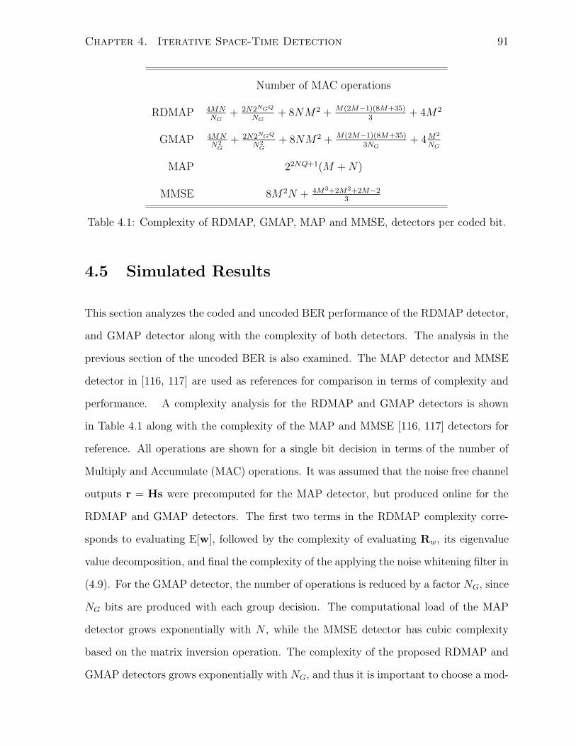
Chapter 4. Iterative Space-Time Detection 91
Number of MAC operations
RDMAP 4MNNG
+ 2N2NGQ
NG+ 8NM 2 + M(2M−1)(8M+35)
3+ 4M2
GMAP 4MNN2
G+ 2N2NGQ
N2G
+ 8NM 2 + M(2M−1)(8M+35)3NG
+ 4M2
NG
MAP 22NQ+1(M + N)
MMSE 8M 2N + 4M3+2M2+2M−23
Table 4.1: Complexity of RDMAP, GMAP, MAP and MMSE, detectors per coded bit.
4.5 Simulated Results
This section analyzes the coded and uncoded BER performance of the RDMAP detector,
and GMAP detector along with the complexity of both detectors. The analysis in the
previous section of the uncoded BER is also examined. The MAP detector and MMSE
detector in [116, 117] are used as references for comparison in terms of complexity and
performance. A complexity analysis for the RDMAP and GMAP detectors is shown
in Table 4.1 along with the complexity of the MAP and MMSE [116, 117] detectors for
reference. All operations are shown for a single bit decision in terms of the number of
Multiply and Accumulate (MAC) operations. It was assumed that the noise free channel
outputs r = Hs were precomputed for the MAP detector, but produced online for the
RDMAP and GMAP detectors. The first two terms in the RDMAP complexity corre-
sponds to evaluating E[w], followed by the complexity of evaluating Rw, its eigenvalue
value decomposition, and final the complexity of the applying the noise whitening filter in
(4.9). For the GMAP detector, the number of operations is reduced by a factor NG, since
NG bits are produced with each group decision. The computational load of the MAP
detector grows exponentially with N , while the MMSE detector has cubic complexity
based on the matrix inversion operation. The complexity of the proposed RDMAP and
GMAP detectors grows exponentially with NG, and thus it is important to choose a mod-
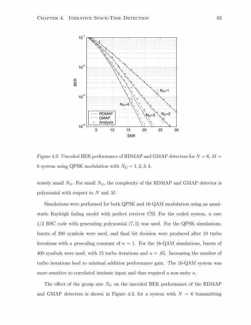
Chapter 4. Iterative Space-Time Detection 92
5 10 15 20 25 3010
-4
10-3
10-2
10-1
RDMAPGMAPAnalysis
NG=1
NG=2NG=3
NG=4
Figure 4.3: Uncoded BER performance of RDMAP and GMAP detectors for N = 6,M =
6 system using QPSK modulation with NG = 1, 2, 3, 4.
erately small NG. For small NG, the complexity of the RDMAP and GMAP detector is
polynomial with respect to N and M .
Simulations were performed for both QPSK and 16-QAM modulation using an quasi-
static Rayleigh fading model with perfect receiver CSI. For the coded system, a rate
1/2 RSC code with generating polynomial (7, 5) was used. For the QPSK simulations,
bursts of 200 symbols were used, and final bit decision were produced after 10 turbo
iterations with a prescaling constant of κ = 1. For the 16-QAM simulations, bursts of
400 symbols were used, with 15 turbo iterations and κ = .65. Increasing the number of
turbo iterations lead to minimal addition performance gain. The 16-QAM system was
more sensitive to correlated intrinsic input and thus required a non-unity κ.
The effect of the group size NG on the uncoded BER performance of the RDMAP
and GMAP detectors is shown in Figure 4.3, for a system with N = 6 transmitting
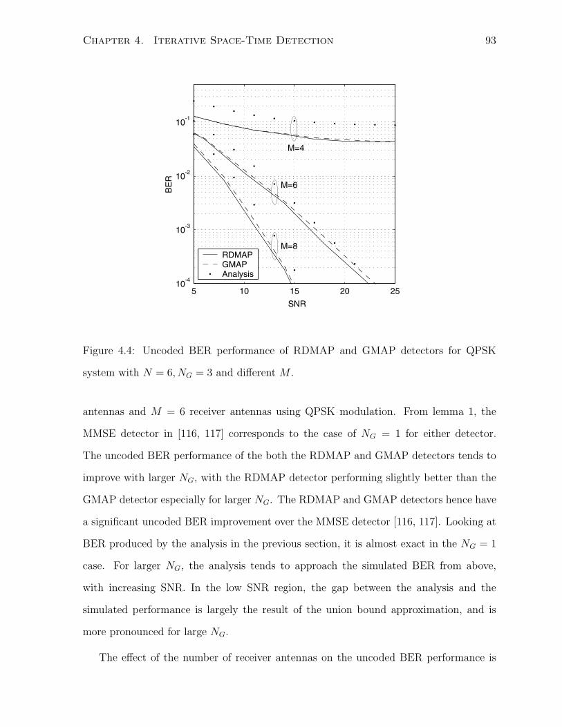
Chapter 4. Iterative Space-Time Detection 93
5 10 15 20 2510
-4
10-3
10-2
10-1
RDMAPGMAPAnalysis
M=4
M=6
M=8
Figure 4.4: Uncoded BER performance of RDMAP and GMAP detectors for QPSK
system with N = 6, NG = 3 and different M .
antennas and M = 6 receiver antennas using QPSK modulation. From lemma 1, the
MMSE detector in [116, 117] corresponds to the case of NG = 1 for either detector.
The uncoded BER performance of the both the RDMAP and GMAP detectors tends to
improve with larger NG, with the RDMAP detector performing slightly better than the
GMAP detector especially for larger NG. The RDMAP and GMAP detectors hence have
a significant uncoded BER improvement over the MMSE detector [116, 117]. Looking at
BER produced by the analysis in the previous section, it is almost exact in the NG = 1
case. For larger NG, the analysis tends to approach the simulated BER from above,
with increasing SNR. In the low SNR region, the gap between the analysis and the
simulated performance is largely the result of the union bound approximation, and is
more pronounced for large NG.
The effect of the number of receiver antennas on the uncoded BER performance is
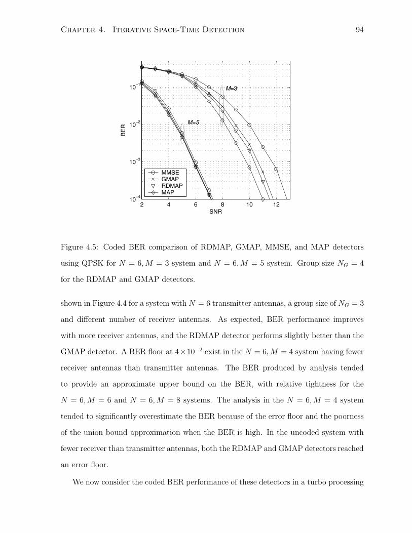
Chapter 4. Iterative Space-Time Detection 94
2 4 6 8 10 1210
−4
10−3
10−2
10−1
SNR
BE
R
MMSEGMAPRDMAPMAP
M 5=
M=3
Figure 4.5: Coded BER comparison of RDMAP, GMAP, MMSE, and MAP detectors
using QPSK for N = 6,M = 3 system and N = 6,M = 5 system. Group size NG = 4
for the RDMAP and GMAP detectors.
shown in Figure 4.4 for a system with N = 6 transmitter antennas, a group size of NG = 3
and different number of receiver antennas. As expected, BER performance improves
with more receiver antennas, and the RDMAP detector performs slightly better than the
GMAP detector. A BER floor at 4×10⁻² exist in the N = 6,M = 4 system having fewer
receiver antennas than transmitter antennas. The BER produced by analysis tended
to provide an approximate upper bound on the BER, with relative tightness for the
N = 6,M = 6 and N = 6,M = 8 systems. The analysis in the N = 6,M = 4 system
tended to significantly overestimate the BER because of the error floor and the poorness
of the union bound approximation when the BER is high. In the uncoded system with
fewer receiver than transmitter antennas, both the RDMAP and GMAP detectors reached
an error floor.
We now consider the coded BER performance of these detectors in a turbo processing

Chapter 4. Iterative Space-Time Detection 95
receiver in systems with fewer receiver antennas than transmitter antennas. For a group
size NG = 4, the BER performance of the RDMAP and GMAP detector is shown in Fig-
ure 4.5 for a N = 6,M = 5 system and a N = 6,M = 3 system. The BER performance
of the MMSE detector from [116, 117] and MAP detector are also shown for reference.
Unlike the uncoded case, there is no error floor, and the turbo processing receiver is
able to equalize both systems that have fewer receiver than transmitter antennas. In
both the N = 6,M = 3 and N = 6,M = 5 systems, the MAP detector performed
the best, the MMSE detector performed the worst and the RDMAP detector preformed
better than the GMAP detector. In the N = 6,M = 5 system, the performance gap
between the MMSE and MAP detector is small, suggesting the MMSE has near optimal
performance. In the N = 6,M = 3 system, however, there is a 2dB performance gap
between the MMSE and MAP detectors, and the RDMAP and GMAP detectors have a
performance improvement of approximately 1.3dB and 1dB respectively, over the MMSE
detector.
The coded BER as a function of the number of turbo iteration is shown in Figure 4.6
for the RDMAP and GMAP detectors with NG = 4 in a N = 6,M = 3 system using
QPSK. The coded BER is produced after 1, 3, 5, and 10 turbo iterations is shown.
For both detectors, there is a significant BER improvement after the first few turbo
iterations, and the incremental improvement is less with each iteration. There is only a
0.3dB performance improvement between the 5th and 10th iteration.
The effect of group size on the coded BER performance of the RDMAP and GMAP
detector is shown in Figure 4.7 as a function of the group size NG = 1, 2, 4, 5 for a system
with N = 10 transmitter antennas and M = 4 receiver antennas using QPSK. The
MAP detector is omitted as it is computational infeasible for this system and the MMSE
detector [116, 117] is equivalent to the case of NG = 1. The BER performance of the
RDMAP and GMAP detectors improves with larger NG, with the RDMAP performing
better than the GMAP detector for a given NG. For the case of NG = 5, the RDMAP and
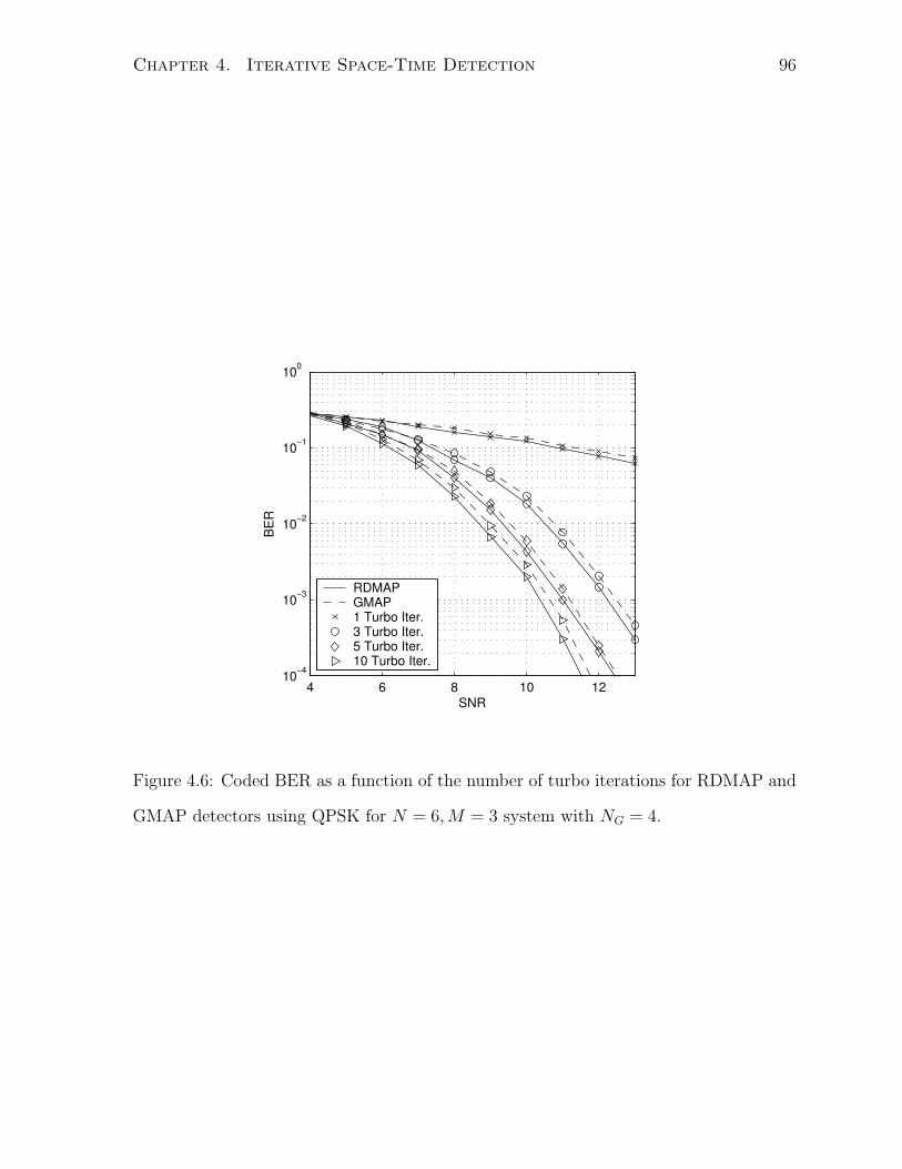
Chapter 4. Iterative Space-Time Detection 96
4 6 8 10 1210−4
10−3
10−2
10−1
100
SNR
BE
R
RDMAPGMAP1 Turbo Iter.3 Turbo Iter.5 Turbo Iter.10 Turbo Iter.
Figure 4.6: Coded BER as a function of the number of turbo iterations for RDMAP and
GMAP detectors using QPSK for N = 6,M = 3 system with NG = 4.
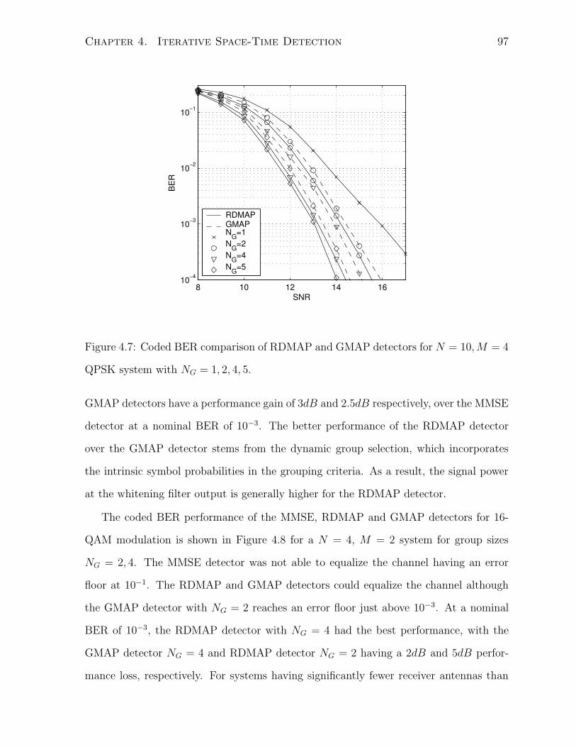
Chapter 4. Iterative Space-Time Detection 97
8 10 12 14 1610−4
10−3
10−2
10−1
SNR
BE
R
RDMAPGMAPNG=1NG=2NG=4NG=5
Figure 4.7: Coded BER comparison of RDMAP and GMAP detectors for N = 10,M = 4
QPSK system with NG = 1, 2, 4, 5.
GMAP detectors have a performance gain of 3dB and 2.5dB respectively, over the MMSE
detector at a nominal BER of 10−3. The better performance of the RDMAP detector
over the GMAP detector stems from the dynamic group selection, which incorporates
the intrinsic symbol probabilities in the grouping criteria. As a result, the signal power
at the whitening filter output is generally higher for the RDMAP detector.
The coded BER performance of the MMSE, RDMAP and GMAP detectors for 16-
QAM modulation is shown in Figure 4.8 for a N = 4, M = 2 system for group sizes
NG = 2, 4. The MMSE detector was not able to equalize the channel having an error
floor at 10−1. The RDMAP and GMAP detectors could equalize the channel although
the GMAP detector with NG = 2 reaches an error floor just above 10−3. At a nominal
BER of 10−3, the RDMAP detector with NG = 4 had the best performance, with the
GMAP detector NG = 4 and RDMAP detector NG = 2 having a 2dB and 5dB perfor-
mance loss, respectively. For systems having significantly fewer receiver antennas than
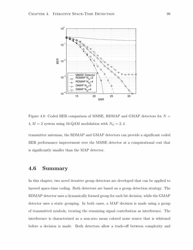
Chapter 4. Iterative Space-Time Detection 98
15 20 25 3010−4
10−3
10−2
10−1
100
SNR
BE
R
MMSE DetectorRDMAP NG=2RDMAP NG=4GMAP NG=2GMAP NG=4
Figure 4.8: Coded BER comparison of MMSE, RDMAP and GMAP detectors for N =
4,M = 2 system using 16-QAM modulation with NG = 2, 4.
transmitter antennas, the RDMAP and GMAP detectors can provide a significant coded
BER performance improvement over the MMSE detector at a computational cost that
is significantly smaller than the MAP detector.
4.6 Summary
In this chapter, two novel iterative group detectors are developed that can be applied to
layered space-time coding. Both detectors are based on a group detection strategy. The
RDMAP detector uses a dynamically formed group for each bit decision, while the GMAP
detector uses a static grouping. In both cases, a MAP decision is made using a group
of transmitted symbols, treating the remaining signal contribution as interference. The
interference is characterized as a non-zero mean colored noise source that is whitened
before a decision is made. Both detectors allow a trade-off between complexity and
Chapter 4. Iterative Space-Time Detection 99
performance through the MAP group size, and include as special cases both the MAP
and MMSE detectors. A novel grouping algorithm is developed for the GMAP detector.
The uncoded BER performance of the RDMAP and GMAP detectors has been analyzed,
and an approximate upper bound on the uncoded BER is provided. In the uncoded case,
the RDMAP and GMAP detectors have a significant performance improvement over the
MMSE detector for a moderately chosen group size. In the coded case, the RDMAP and
GMAP detectors can have a large performance improvement over the MMSE detector in
spatially multiplexed systems having fewer receiver antennas than transmitter antennas.
Chapter 5
Space-Time Coding Over Slow
Fading Channels
This chapter examines the design of coded modulation systems in to slow and quasi-static
fading scenarios. Mapping and precoding strategies are proposed to mitigate slow fading
effects. The coded modulation and detection strategies developed in previous chapters
are used where applicable.
5.1 Introduction
The adverse effects of slow and quasi-static fading can be mitigated through multi-
dimensional mapping and by the introduction of a spatial precoder. The simplest pre-
coder is a time-varying spatial interleaver, which is employed in the D-BLAST structure.
A more general class of spatial precoders is based on unitary transformation matrices
that rotate the symbol constellation at arbitrary angles [36, 37, 38, 39, 40, 41, 42]. Fade
resistent unitary transformations are often determined through algebraic number the-
ory [122]. Unitary precoding can be used in either MLCM or BICM transmissions and
does not significantly affect receiver complexity sinceas it is a linear transformation. A
wide range of detectors can thus be applied such as the MMSE detector, APP detector,
100
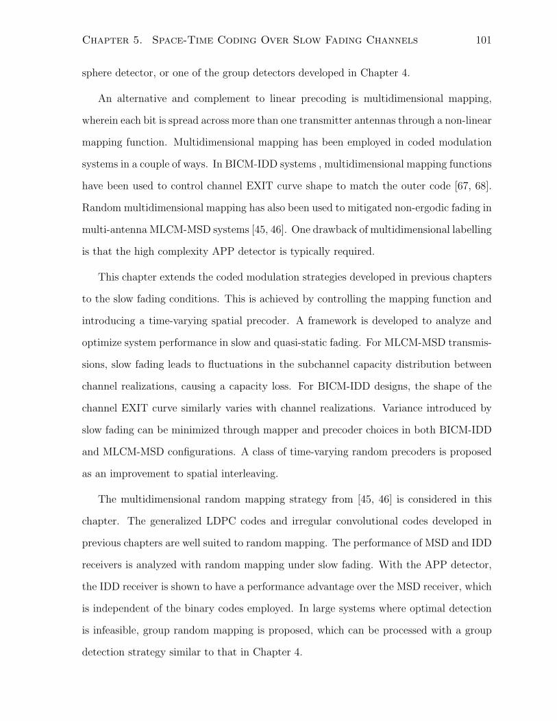
Chapter 5. Space-Time Coding Over Slow Fading Channels 101
sphere detector, or one of the group detectors developed in Chapter 4.
An alternative and complement to linear precoding is multidimensional mapping,
wherein each bit is spread across more than one transmitter antennas through a non-linear
mapping function. Multidimensional mapping has been employed in coded modulation
systems in a couple of ways. In BICM-IDD systems , multidimensional mapping functions
have been used to control channel EXIT curve shape to match the outer code [67, 68].
Random multidimensional mapping has also been used to mitigated non-ergodic fading in
multi-antenna MLCM-MSD systems [45, 46]. One drawback of multidimensional labelling
is that the high complexity APP detector is typically required.
This chapter extends the coded modulation strategies developed in previous chapters
to the slow fading conditions. This is achieved by controlling the mapping function and
introducing a time-varying spatial precoder. A framework is developed to analyze and
optimize system performance in slow and quasi-static fading. For MLCM-MSD transmis-
sions, slow fading leads to fluctuations in the subchannel capacity distribution between
channel realizations, causing a capacity loss. For BICM-IDD designs, the shape of the
channel EXIT curve similarly varies with channel realizations. Variance introduced by
slow fading can be minimized through mapper and precoder choices in both BICM-IDD
and MLCM-MSD configurations. A class of time-varying random precoders is proposed
as an improvement to spatial interleaving.
The multidimensional random mapping strategy from [45, 46] is considered in this
chapter. The generalized LDPC codes and irregular convolutional codes developed in
previous chapters are well suited to random mapping. The performance of MSD and IDD
receivers is analyzed with random mapping under slow fading. With the APP detector,
the IDD receiver is shown to have a performance advantage over the MSD receiver, which
is independent of the binary codes employed. In large systems where optimal detection
is infeasible, group random mapping is proposed, which can be processed with a group
detection strategy similar to that in Chapter 4.
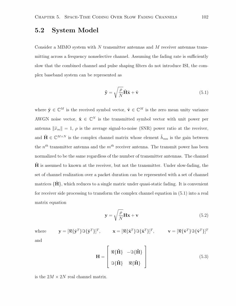
Chapter 5. Space-Time Coding Over Slow Fading Channels 102
5.2 System Model
Consider a MIMO system with N transmitter antennas and M receiver antennas trans-
mitting across a frequency nonselective channel. Assuming the fading rate is sufficiently
slow that the combined channel and pulse shaping filters do not introduce ISI, the com-
plex baseband system can be represented as
y =
√
ρ
NHx + v (5.1)
where y ∈ CM is the received symbol vector, v ∈ C
M is the zero mean unity variance
AWGN noise vector, x ∈ CN is the transmitted symbol vector with unit power per
antenna ‖xm‖ = 1, ρ is the average signal-to-noise (SNR) power ratio at the receiver,
and H ∈ CM×N is the complex channel matrix whose element hmn is the gain between
the nth transmitter antenna and the mth receiver antenna. The transmit power has been
normalized to be the same regardless of the number of transmitter antennas. The channel
H is assumed to known at the receiver, but not the transmitter. Under slow-fading, the
set of channel realization over a packet duration can be represented with a set of channel
matrices H, which reduces to a single matric under quasi-static fading. It is convenient
for receiver side processing to transform the complex channel equation in (5.1) into a real
matrix equation
y =
√
ρ
NHx + v (5.2)
where y = [<yT=yT]T , x = [<xT=xT]T , v = [<vT=vT]T
and
H =
<H −=H
=H <H
(5.3)
is the 2M × 2N real channel matrix.
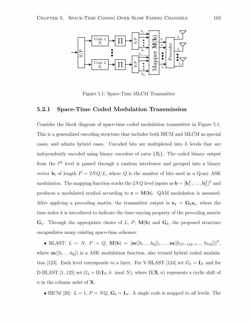
Chapter 5. Space-Time Coding Over Slow Fading Channels 103
S/P
Code 1R1
P S/P
b1
bP
Code L
RL
P
b( -1) +1L P
bLP
S/P
Mapper
()
Mb
x1
x2
xN
s1
s2
sN
Pre
coder
Figure 5.1: Space-Time MLCM Transmitter
5.2.1 Space-Time Coded Modulation Transmission
Consider the block diagram of space-time coded modulation transmitter in Figure 5.1.
This is a generalized encoding structure that includes both BICM and MLCM as special
cases, and admits hybrid cases. Uncoded bits are multiplexed into L levels that are
independently encoded using binary encoders of rates Rl. The coded binary output
from the lth level is passed through a random interleaver and grouped into a binary
vector bl of length P = 2NQ/L, where Q is the number of bits used in a Q-ary ASK
modulation. The mapping function stacks the 2NQ level inputs as b = [bT1 , . . . ,bT
L]T and
produces a modulated symbol according to s = M(b). QAM modulation is assumed.
After applying a precoding matrix, the transmitter output is xk = Gksk, where the
time index k is introduced to indicate the time-varying property of the precoding matrix
Gk. Through the appropriate choice of L, P , M(b) and Gk, the proposed structure
encapsulates many existing space-time schemes:
• BLAST: L = N , P = Q, M(b) = [m([b1 . . . bQ]), . . . ,m([b(N−1)Q−1 . . . bNQ])]T ,
where m([b1 . . . bQ]) is a ASK modulation function, also termed hybrid coded modula-
tion [123]. Each level corresponds to a layer. For V-BLAST [124] set Gk = IN and for
D-BLAST [1, 125] set Gk = Π(IN , k mod N), where Π(X, n) represents a cyclic shift of
n in the column order of X.
• BICM [20]: L = 1, P = NQ, Gk = IN . A single code is mapped to all levels. The
Chapter 5. Space-Time Coding Over Slow Fading Channels 104
mapping function M(b) can be an ASK, or multidimensional QAM [67, 68].
• MLCM: L = NQ, P = 1, Gk = IN . An independent code is used for each level.
The mapping function M(b) can be ASK [123, 126] or multidimensional QAM [45, 46].
• Multilevel BICM(ML-BICM) [127]: L = 2Q, P = N/2, Gk = IN , M(b) =
[m([c1 . . . c2Q]), . . . ,m([c(N/2−1)2Q−1 . . . cNQ])]T , cn = b(N−1)mod(n,Q)+dn/Qe. Also know as
multilevel coding with spatial multiplexing [128]. Each code is spatially multiplexed and
mapped to a particular bit position in a QAM modulation. A slight variation of ML-
BICM is Q-staged BICM [129], which maps bits from a common subcode to the same
bit position in the in-phase and quadrature-phase signal components.
Random MQAM labelling is form multidimensional QAM labelling that is suited to
slow-fading conditions [45, 46]. As discussed in Chapter 3, random MQAM is formed
using a pseudo-random lookup table that assign an arbitrary mapping between binary
vectors and constellation points. This mapping function changes between symbols and
is known at the receiver.
5.2.2 Space-Time Receiver
The MSD and IDD receiver structures discussed in previous chapters will be considered.
The use multi-dimensional mapping in this chapter puts some limitations on the detector
choice, particularly with group detection. The group detectors in Chapter 4 were derived
for ASK modulation without spatial precoding. Random precoding requires a group
selection algorithm to be applied each symbol, adding additional complexity unless a
fixed grouping is used. Multidimensional mapping schemes generally contain non-linear
bit groupings that cannot be separated by linear filtering and must be grouped together in
the detector processing. The group detector is derived as follows for non-ASK labelling.
Consider using a detector group size of NG, and a possibly multi-dimensional mapping
function m(b) whose output spans MG complex dimensions. We assume NG is a multiple
of MG and let NG = 2NQ−NG be the size of the detector interfering group. Combining
Chapter 5. Space-Time Coding Over Slow Fading Channels 105
the channel and precoder matrix C = HGk, the channel output can be expressed as
r = CGsG + CGsG + v (5.4)
similarly to (4.6). The contribution of the complementary group and Gaussian noise is
treated as a colored noise source. Let w = CisG+v be a colored noise source whose mean
and variance can be evaluated by partitioning the symbol interference vector as sG =
[sG1, . . . , sGNG/MG] where sGi = m(b). The noise mean is w = E[w] =
∑NG/MG
j=1 CGj sGj,
where CGj are the columns of CG corresponding to sGj, and the covariance matrix is
Rw =∑NG/MG
j=1 CGjΩjCTGj
+ Iσ2/2, where Ωj = E[|sGj − sGj|2] = E[s2Gj
]− E[sGj]2. The
expectation of the nth moment of sGj can be evaluated as
snGj = E[sn
Gj] =∑
bj∈BMG
MG∏
l=1
(m(bj))n bl exp(λI [bl]) + bl
1 + exp(λI [bl])(5.5)
The noise w can be whitened by first removing the mean w and then applying an ap-
propriate noise whitening filter F = Σ−1/2QT , where Σ is a diagonal matrix and Q
is an orthogonal matrix, both obtained from the eigenvalue decomposition of Rw =
QΣQT ,QQT = I. The noise whitened channel observation is given by r = F(y − w)
and the detector output for the lth bit in the binary group vector bG is given by
λE[bGl] = log
∑
bG:bGl=1 exp(
−‖r−CGmG(bG)‖2
2
)
+∑
m log bGmeλI [bGm]+bGm
1+eλI [bGm]
∑
bG:bGl=0 exp(
−‖r−CGmG(b)‖2
2
)
+∑
m log bGmeλi[bGm]+bGm
1+eλI [bGm]
− λi[bGl] (5.6)
where mG is the arrogate mapping function for the symbols in the group vector.
The GMAP group selection algorithm from Chapter 4 can be applied with non-ASK
modulation by modifying the channel correlation matrix R that is used for GMAP group
selection. Let θ be a set of MG integers representing indices of the vector s that are
spatially correlated with a group-wise mapping function. Setting all entries of R to zero,
where both the row and column indices are in θ, ensures that the mapping group takes
precedence over other groupings. This preprocessing must be applied for all mapping
groups in the symbol vector before the GMAP group selection algorithm can be applied.
Chapter 5. Space-Time Coding Over Slow Fading Channels 106
5.3 Space-Time MLCM Design
MLCM was introduced in Chapter 2 using GLDPC component codes and MSD decoding
over the AWGN channel. Over ergodic fading channels, the total capacity, and subchan-
nel capacity distribution is relatively constant between channel uses. Under slow fading,
the average channel capacity over a packet is not constant and therefore the subchannel
capacities are random entities. A different rate optimization is required to determine
subcode rates based on the underlying channel statistics.
The instantaneous unconstrained MIMO channel capacity is CU = log det[IM +
ρNHHH ] bps/Hz [1]. For discrete modulation, the modulation constrained capacity of a
MIMO fading channel is given by
CCM = I(s; r) = H(s)− Es,r
(
log2
∑
s′∈S p(r|s)p(r|s)
)
(5.7)
= NQ− Es,r
(
log2
∑
s′∈S exp(‖r−√
ρNHs′‖2/2)
exp(‖r−√
ρNHs‖2/2)
)
(5.8)
where S is the set of possible transmitted symbols, and equiprobable transmitted symbols
and perfect receiver CSI are assumed. For packet based transmission, it is also useful to
define the packet averaged channel capacities CU = EH[CU ] and CCM = EH[CCM ], where
the expectation is taken over the set channel realizations seen over a packet. In quasi-
static fading, the instantaneous and packet averaged capacities have the same statistics,
since the channel remains constant for the packet duration. The instantaneous CM
capacity can be decomposed into L parallel subchannels using the chain rule of mutual
information as:
I(b;y) = I(b1;y) + I(b2;y|b1) + . . . + I(bL;y|b1, . . . ,bL−1) (5.9)
where Cl = I(bl;y|b1, . . . ,bl−1) is the channel capacity associated with the lth symbol
bit, assuming lower level bits are known. Averaging subchannel capacities over a packet
yields Cl = E[Cl]. Over a slow fading channel, the subchannel capacities are random
entities whose statistics are influenced by the packet length and fading rates.
Chapter 5. Space-Time Coding Over Slow Fading Channels 107
For the slow fading channel, the decomposition in (5.9) produces subchannel rates
that vary with channel realizations, thus a set of rates that achieves capacity for one
channel realization may not for another. Since there is no one rate distribution that
achieves capacity for all channel realizations, we choose a distribution that leads to error-
free transmission on as many channel realizations as possible. Let fER(rl, ρ) represent
FER as a function of the code rates rl and SNR ρ, and let PER be the design error
rate. A frame or packet error is declared if there is an error in any of the levels. The
optimal set of rates can be found by solving the following optimization problem:
maxL∑
l=1
rl s.t. fER(rl, ρ) ≤ PER, rl > 0 ∀ l (5.10)
In [61], the solution to (5.10) is found by assuming that level errors occur indepen-
dently, in which case, the optimal set of rates r∗l is determined by the condition,
P lER(ρ, r∗l ) = P 1
ER(ρ, r∗1), ∀ l, where is P lER(ρ, r∗l ) is the error rate for the lth level. Unfor-
tunately, level errors are not independent since an error on one level indicates the channel
may be in deep fade, which would also tend to cause errors in other levels. It follows that
solving (5.10) directly leads to better performance than assuming independent level er-
rors. Since (5.10) is usually evaluated over a finite set of channel realizations, fER(rl, ρ)
is not a smooth function and so gradient based optimization techniques lead to unstable
results. A steepest decent optimization procedure not based on gradients can be used
to solve (5.10) by controlling the step-size, and noting that fER(rl, ρ) is monotonically
increasing function of rl and thus has no local minima or maxima. A general approach
to solving (5.10) is to increase the rate which least affects the FER for a fixed step size;
if none of the rates can be further incremented, reduce the step-size and all the rates by
the old step size, and continue. An algorithm to solve (5.10) based on this strategy can
be found in Appendix A.3.
The optimization problem in (5.10) is useful for finding an optimal set of rates for
different design parameters such as precoders, mapping functions and code structures. It
does not, however, give insight into why certain design choices work better than others.
Chapter 5. Space-Time Coding Over Slow Fading Channels 108
One way to visualize the performance of the multi-antenna MLCM transmissions is to
look at the subchannel capacities ci as a function of the CM capacity CCM(ρ, H). It is
argued in [45, 46] that for an MLCM-MSD transmission to achieve the channel capacity
over a quasi-static fading channel, the subchannel capacities must be a deterministic
function of the CM capacity as
Cl(ρ, H) = gl(CCM(ρ, H)) (5.11)
The proof for (5.11) is found in [46]. Equation (5.11) essentially states that there should
be no variation in the distribution of subchannel capacities once the overall capacity
is fixed. Although random mapping was found to minimizes the variance in the gl(C)
functions, these functions are in general probabilistic, with variations that depend on
the particular channel realization. A small variance in the gl(C) functions means that
different levels are tightly correlated and so either none of the subchannels are in outage,
or all or most of the subchannels are in outage. A large variance in the gl(C) functions
leads to poor performance since no one set of component code rates will operate close to
capacity for different channel realizations.
5.3.1 Precoder Design
The precoder in a space-time MLCM transmission serves two purposes. Spectral pre-
coders are traditionally used to minimize degradation of the CM capacity due to a poor
alignment between the constellation and channel realization that may arise under slow
and quasi-static fading conditions. A second and ostensibly more important precoder
function in MLCM-MSD transmissions is to spread each bit across the signal space. The
CM capacity is decomposed into a set of random subchannel capacities under staged de-
coding. Precoding can be used to reduce variance in these subchannel capacity functions
thereby improving performance.
As a natural starting point, consider how the unconstrained channel capacity is af-
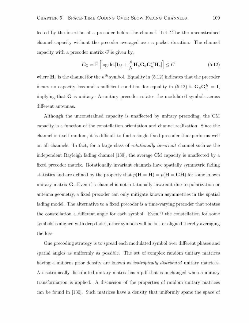
Chapter 5. Space-Time Coding Over Slow Fading Channels 109
fected by the insertion of a precoder before the channel. Let C be the unconstrained
channel capacity without the precoder averaged over a packet duration. The channel
capacity with a precoder matrix G is given by,
CG = E[
log det[IM +ρ
NHnGnG
Hn Hn]
]
≤ C (5.12)
where Hn is the channel for the nth symbol. Equality in (5.12) indicates that the precoder
incurs no capacity loss and a sufficient condition for equality in (5.12) is GnGHn = I,
implying that G is unitary. A unitary precoder rotates the modulated symbols across
different antennas.
Although the unconstrained capacity is unaffected by unitary precoding, the CM
capacity is a function of the constellation orientation and channel realization. Since the
channel is itself random, it is difficult to find a single fixed precoder that performs well
on all channels. In fact, for a large class of rotationally invariant channel such as the
independent Rayleigh fading channel [130], the average CM capacity is unaffected by a
fixed precoder matrix. Rotationally invariant channels have spatially symmetric fading
statistics and are defined by the property that p(H = H) = p(H = GH) for some known
unitary matrix G. Even if a channel is not rotationally invariant due to polarization or
antenna geometry, a fixed precoder can only mitigate known asymmetries in the spatial
fading model. The alternative to a fixed precoder is a time-varying precoder that rotates
the constellation a different angle for each symbol. Even if the constellation for some
symbols is aligned with deep fades, other symbols will be better aligned thereby averaging
the loss.
One precoding strategy is to spread each modulated symbol over different phases and
spatial angles as uniformly as possible. The set of complex random unitary matrices
having a uniform prior density are known as isotropically distributed unitary matrices.
An isotropically distributed unitary matrix has a pdf that is unchanged when a unitary
transformation is applied. A discussion of the properties of random unitary matrices
can be found in [130]. Such matrices have a density that uniformly spans the space of
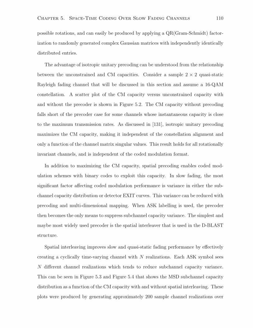
Chapter 5. Space-Time Coding Over Slow Fading Channels 110
possible rotations, and can easily be produced by applying a QR(Gram-Schmidt) factor-
ization to randomly generated complex Gaussian matrices with independently identically
distributed entries.
The advantage of isotropic unitary precoding can be understood from the relationship
between the unconstrained and CM capacities. Consider a sample 2 × 2 quasi-static
Rayleigh fading channel that will be discussed in this section and assume a 16-QAM
constellation. A scatter plot of the CM capacity versus unconstrained capacity with
and without the precoder is shown in Figure 5.2. The CM capacity without precoding
falls short of the precoder case for some channels whose instantaneous capacity is close
to the maximum transmission rates. As discussed in [131], isotropic unitary precoding
maximizes the CM capacity, making it independent of the constellation alignment and
only a function of the channel matrix singular values. This result holds for all rotationally
invariant channels, and is independent of the coded modulation format.
In addition to maximizing the CM capacity, spatial precoding enables coded mod-
ulation schemes with binary codes to exploit this capacity. In slow fading, the most
significant factor affecting coded modulation performance is variance in either the sub-
channel capacity distribution or detector EXIT curves. This variance can be reduced with
precoding and multi-dimensional mapping. When ASK labelling is used, the precoder
then becomes the only means to suppress subchannel capacity variance. The simplest and
maybe most widely used precoder is the spatial interleaver that is used in the D-BLAST
structure.
Spatial interleaving improves slow and quasi-static fading performance by effectively
creating a cyclically time-varying channel with N realizations. Each ASK symbol sees
N different channel realizations which tends to reduce subchannel capacity variance.
This can be seen in Figure 5.3 and Figure 5.4 that shows the MSD subchannel capacity
distribution as a function of the CM capacity with and without spatial interleaving. These
plots were produced by generating approximately 200 sample channel realizations over
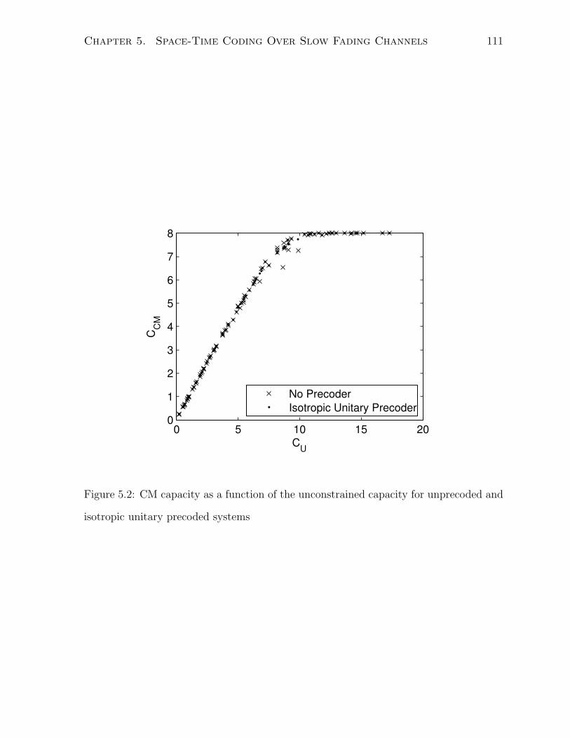
Chapter 5. Space-Time Coding Over Slow Fading Channels 111
0 5 10 15 200
1
2
3
4
5
6
7
8
CU
CC
M
No PrecoderIsotropic Unitary Precoder
Figure 5.2: CM capacity as a function of the unconstrained capacity for unprecoded and
isotropic unitary precoded systems
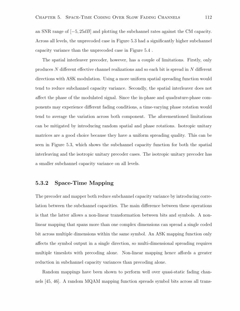
Chapter 5. Space-Time Coding Over Slow Fading Channels 112
an SNR range of [−5, 25dB] and plotting the subchannel rates against the CM capacity.
Across all levels, the unprecoded case in Figure 5.3 had a significantly higher subchannel
capacity variance than the unprecoded case in Figure 5.4 .
The spatial interleaver precoder, however, has a couple of limitations. Firstly, only
produces N different effective channel realizations and so each bit is spread in N different
directions with ASK modulation. Using a more uniform spatial spreading function would
tend to reduce subchannel capacity variance. Secondly, the spatial interleaver does not
affect the phase of the modulated signal. Since the in-phase and quadrature-phase com-
ponents may experience different fading conditions, a time-varying phase rotation would
tend to average the variation across both component. The aforementioned limitations
can be mitigated by introducing random spatial and phase rotations. Isotropic unitary
matrices are a good choice because they have a uniform spreading quality. This can be
seen in Figure 5.3, which shows the subchannel capacity function for both the spatial
interleaving and the isotropic unitary precoder cases. The isotropic unitary precoder has
a smaller subchannel capacity variance on all levels.
5.3.2 Space-Time Mapping
The precoder and mapper both reduce subchannel capacity variance by introducing corre-
lation between the subchannel capacities. The main difference between these operations
is that the latter allows a non-linear transformation between bits and symbols. A non-
linear mapping that spans more than one complex dimensions can spread a single coded
bit across multiple dimensions within the same symbol. An ASK mapping function only
affects the symbol output in a single direction, so multi-dimensional spreading requires
multiple timeslots with precoding alone. Non-linear mapping hence affords a greater
reduction in subchannel capacity variances than precoding alone.
Random mappings have been shown to perform well over quasi-static fading chan-
nels [45, 46]. A random MQAM mapping function spreads symbol bits across all trans-
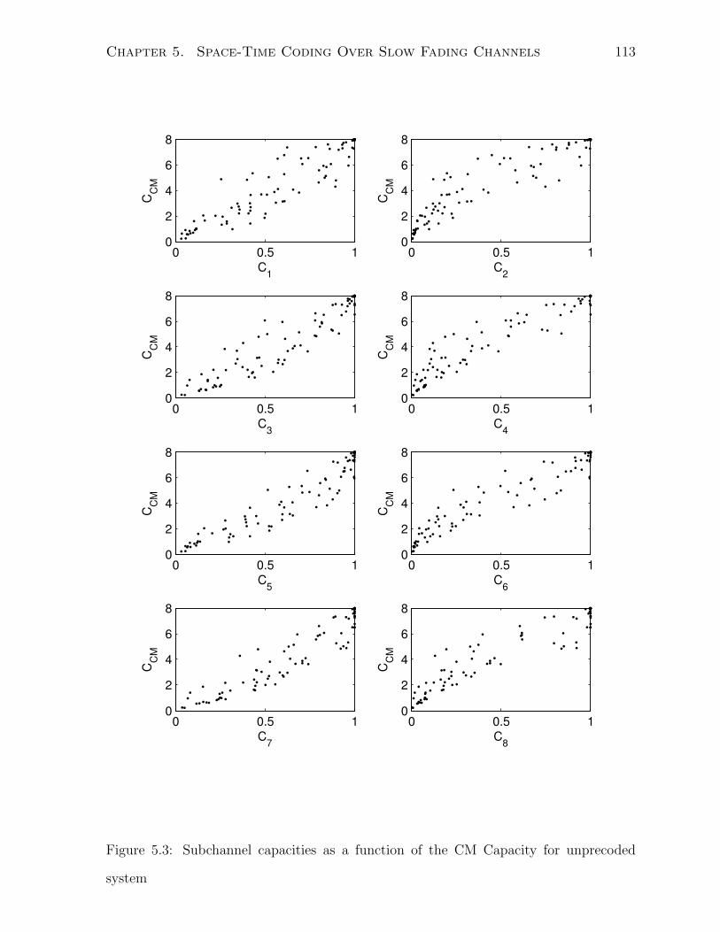
Chapter 5. Space-Time Coding Over Slow Fading Channels 113
0 0.5 10
2
4
6
8
C1
CC
M
0 0.5 10
2
4
6
8
C2
CC
M
0 0.5 10
2
4
6
8
C3
CC
M
0 0.5 10
2
4
6
8
C4
CC
M
0 0.5 10
2
4
6
8
C5
CC
M
0 0.5 10
2
4
6
8
C6
CC
M
0 0.5 10
2
4
6
8
C7
CC
M
0 0.5 10
2
4
6
8
C8
CC
M
Figure 5.3: Subchannel capacities as a function of the CM Capacity for unprecoded
system
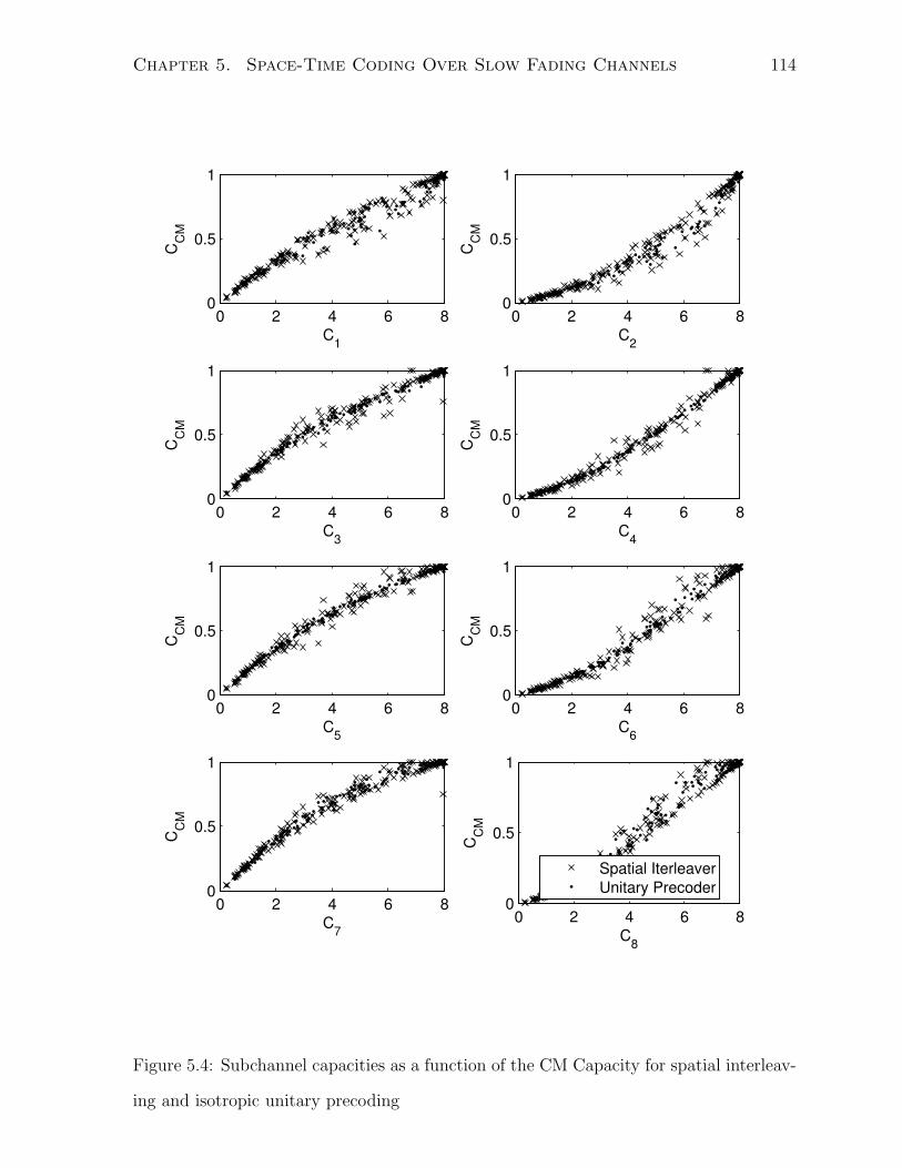
Chapter 5. Space-Time Coding Over Slow Fading Channels 114
0 2 4 6 80
0.5
1
C1
CC
M
0 2 4 6 80
0.5
1
C2
CC
M
0 2 4 6 80
0.5
1
C3
CC
M
0 2 4 6 80
0.5
1
C4
CC
M
0 2 4 6 80
0.5
1
C5
CC
M
0 2 4 6 80
0.5
1
C6
CC
M
0 2 4 6 80
0.5
1
C7
CC
M
0 2 4 6 80
0.5
1
C8
CC
M
Spatial IterleaverUnitary Precoder
Figure 5.4: Subchannel capacities as a function of the CM Capacity for spatial interleav-
ing and isotropic unitary precoding
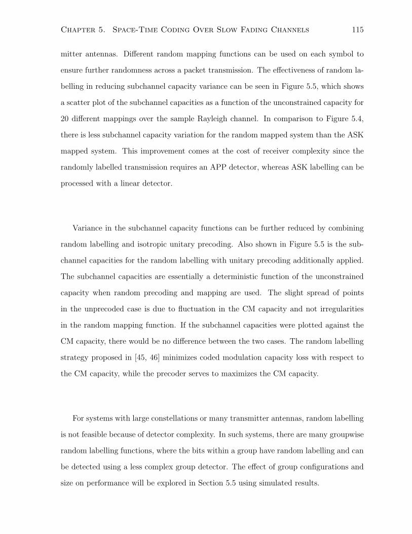
Chapter 5. Space-Time Coding Over Slow Fading Channels 115
mitter antennas. Different random mapping functions can be used on each symbol to
ensure further randomness across a packet transmission. The effectiveness of random la-
belling in reducing subchannel capacity variance can be seen in Figure 5.5, which shows
a scatter plot of the subchannel capacities as a function of the unconstrained capacity for
20 different mappings over the sample Rayleigh channel. In comparison to Figure 5.4,
there is less subchannel capacity variation for the random mapped system than the ASK
mapped system. This improvement comes at the cost of receiver complexity since the
randomly labelled transmission requires an APP detector, whereas ASK labelling can be
processed with a linear detector.
Variance in the subchannel capacity functions can be further reduced by combining
random labelling and isotropic unitary precoding. Also shown in Figure 5.5 is the sub-
channel capacities for the random labelling with unitary precoding additionally applied.
The subchannel capacities are essentially a deterministic function of the unconstrained
capacity when random precoding and mapping are used. The slight spread of points
in the unprecoded case is due to fluctuation in the CM capacity and not irregularities
in the random mapping function. If the subchannel capacities were plotted against the
CM capacity, there would be no difference between the two cases. The random labelling
strategy proposed in [45, 46] minimizes coded modulation capacity loss with respect to
the CM capacity, while the precoder serves to maximizes the CM capacity.
For systems with large constellations or many transmitter antennas, random labelling
is not feasible because of detector complexity. In such systems, there are many groupwise
random labelling functions, where the bits within a group have random labelling and can
be detected using a less complex group detector. The effect of group configurations and
size on performance will be explored in Section 5.5 using simulated results.
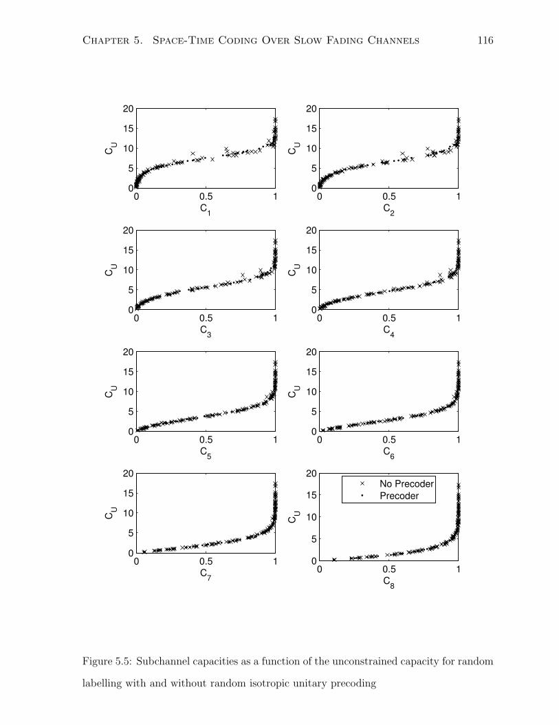
Chapter 5. Space-Time Coding Over Slow Fading Channels 116
0 0.5 10
5
10
15
20
C1
CU
0 0.5 10
5
10
15
20
C2
CU
0 0.5 10
5
10
15
20
C3
CU
0 0.5 10
5
10
15
20
C4
CU
0 0.5 10
5
10
15
20
C5
CU
0 0.5 10
5
10
15
20
C6
CU
0 0.5 10
5
10
15
20
C7
CU
0 0.5 10
5
10
15
20
C8
CU
No PrecoderPrecoder
Figure 5.5: Subchannel capacities as a function of the unconstrained capacity for random
labelling with and without random isotropic unitary precoding

Chapter 5. Space-Time Coding Over Slow Fading Channels 117
5.4 Space-Time Iterative Receiver Design
Thus far design parameters such as the binary codes, precoder and symbol mapping have
been analyzed for MLCM-MSD systems. In this section, these design parameters will be
analyze under IDD receiver processing.
5.4.1 MLCM Rate Allocation
An IDD strategy uses iterative message passing to approximate the Maximum Likelihood
(ML) decoder. It is shown in [8] that if an ML decoder is used, an MLCM-MSD scheme
can achieve error-free transmission for a set of rates other than those in (5.10), if the
following conditions are satisfied:
L∑
l=1
rl < CCM
rα1 + . . . + rαn ≤ I(y; bαi|bαj
) ∀ n, αn ∈ Sn (5.13)
where Sn is a subset of 1, . . . , L having n unique elements and αj is the comple-
mentary set of αi such that αi ∪ αj = 1, . . . , L and αi ∩ αj = ∅. In order
to choose these rates, consider the following theorem:
Theorem 1: For any channel realizations whose CM capacity is greater than or
equal to the transmission rate, an asymptotically long MLCM-MSD transmission with
random mapping can achieve error-free transmission for an equal rate assignment if the
ML decoder is applied.
proof: This is proven using the set of conditions in (5.13). If a particular channel
realization is not in outage, then the first condition in (5.13) is satisfied. Expanding the
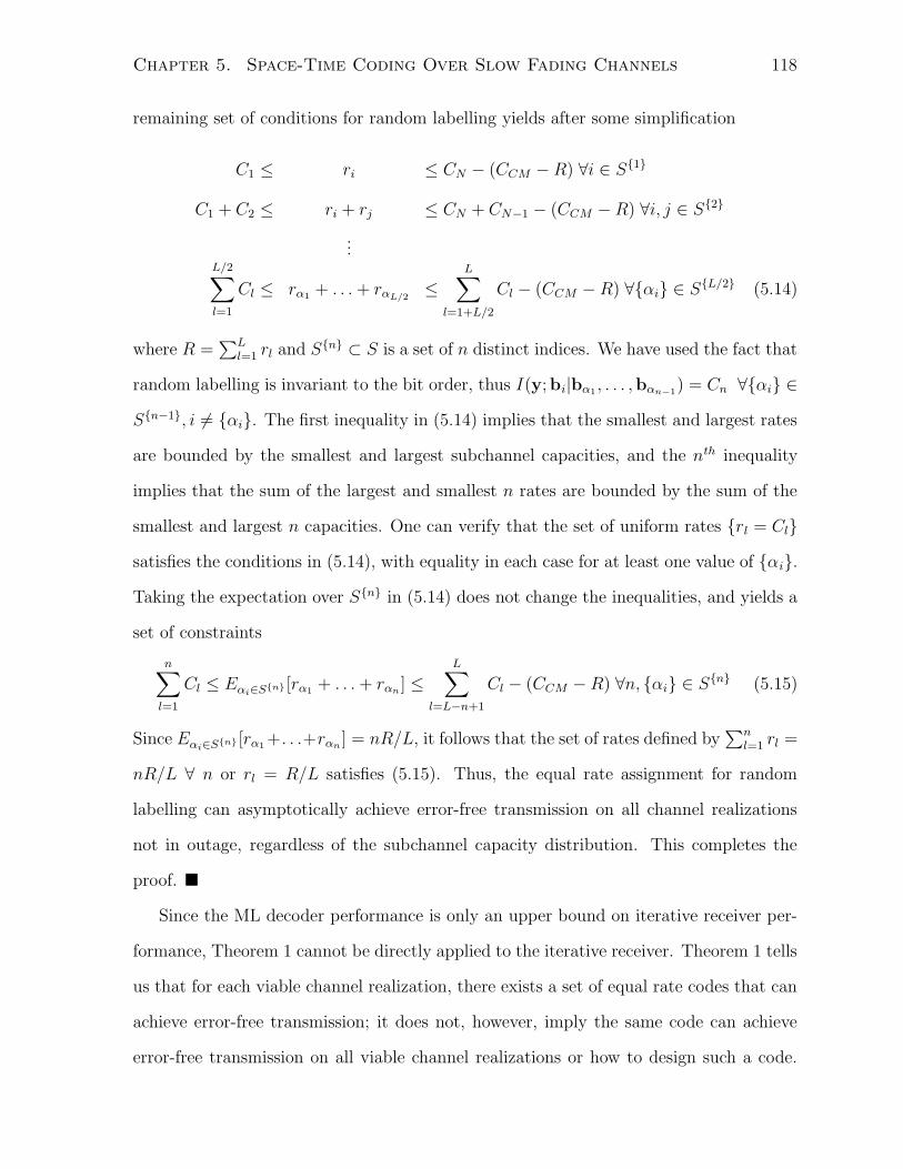
Chapter 5. Space-Time Coding Over Slow Fading Channels 118
remaining set of conditions for random labelling yields after some simplification
C1 ≤ ri ≤ CN − (CCM −R) ∀i ∈ S1
C1 + C2 ≤ ri + rj ≤ CN + CN−1 − (CCM −R) ∀i, j ∈ S2
...L/2∑
l=1
Cl ≤ rα1 + . . . + rαL/2≤
L∑
l=1+L/2
Cl − (CCM −R) ∀αi ∈ SL/2 (5.14)
where R =∑L
l=1 rl and Sn ⊂ S is a set of n distinct indices. We have used the fact that
random labelling is invariant to the bit order, thus I(y;bi|bα1 , . . . ,bαn−1) = Cn ∀αi ∈
Sn−1, i 6= αi. The first inequality in (5.14) implies that the smallest and largest rates
are bounded by the smallest and largest subchannel capacities, and the nth inequality
implies that the sum of the largest and smallest n rates are bounded by the sum of the
smallest and largest n capacities. One can verify that the set of uniform rates rl = Cl
satisfies the conditions in (5.14), with equality in each case for at least one value of αi.
Taking the expectation over Sn in (5.14) does not change the inequalities, and yields a
set of constraints
n∑
l=1
Cl ≤ Eαi∈Sn [rα1 + . . . + rαn ] ≤L∑
l=L−n+1
Cl − (CCM −R) ∀n, αi ∈ Sn (5.15)
Since Eαi∈Sn [rα1 +. . .+rαn ] = nR/L, it follows that the set of rates defined by∑n
l=1 rl =
nR/L ∀ n or rl = R/L satisfies (5.15). Thus, the equal rate assignment for random
labelling can asymptotically achieve error-free transmission on all channel realizations
not in outage, regardless of the subchannel capacity distribution. This completes the
proof.
Since the ML decoder performance is only an upper bound on iterative receiver per-
formance, Theorem 1 cannot be directly applied to the iterative receiver. Theorem 1 tells
us that for each viable channel realization, there exists a set of equal rate codes that can
achieve error-free transmission; it does not, however, imply the same code can achieve
error-free transmission on all viable channel realizations or how to design such a code.

Chapter 5. Space-Time Coding Over Slow Fading Channels 119
An equal rate assignment is a good design rule since it facilitates a simple 2-dimensional
EXIT chart analysis. Multi-rate assignments require multi-dimensional EXIT charts that
are more difficult to analyze in practice [127]. For an equal rate assignment using iden-
tical codes, the code design procedure for MLCM and BICM systems is identical under
IDD processing.
5.4.2 EXIT Chart Analysis
Over the AWGN and ergodic Rayleigh fading channels, the detector EXIT curve is con-
stant between channel realizations, leading to a code profile that is asymptotically capac-
ity achieving for all channel realizations. Under slow fading, the detector EXIT curve is
not constant and varies with individual channel realizations. In addition, the distribution
of detector EXIT curves is dependent on the number of symbols used to evaluate the
channel message mutual information. A decode EXIT curve may intersect the detector
curve for a certain fraction of channel realizations: this fraction becomes the predicted
FER. Thus, the outer code rate needs to be maximized while maintaining a minimal level
of FER performance. This optimization can be divided into two steps. The first step
is to determine a design channel EXIT curve Ich∗E (Ich
I ) irrespective of the binary code.
The area under the design channel curve is maximized such that the fraction of channel
realizations leading to intersections does not exceed the prescribed FER. The second step
is to construct the outer code based on the design channel EXIT curve. The EXIT chart
code design procedures developed in Chapter 2 and Chapter 3 can be directly applied to
the design curve produced from the first step.
A design channel curve that minimizes the FER can found by evaluating I chI at points
xi ∈ [0 1] and solving the following optimization problem:
arg maxIch∗E (xi)
∑
i
Ich∗E (xi) s.t. fER(xi, ρ) ≤ PER, Ich∗
E (xi) > Ich∗E (xj) > 0 ∀ xi > xj,
(5.16)
where fER(xi, ρ) = EH[∏
xiI(Ich∗
E (xi) < IchE (xi,H, ρ))], and I(x) is an indicator function
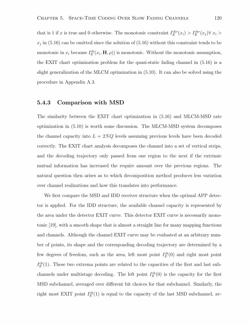
Chapter 5. Space-Time Coding Over Slow Fading Channels 120
that is 1 if x is true and 0 otherwise. The monotonic constraint I ch∗E (xi) > Ich∗
E (xj)∀ xi >
xj in (5.16) can be omitted since the solution of (5.16) without this constraint tends to be
monotonic in xi because IchE (xi,H, ρ)) is monotonic. Without the monotonic assumption,
the EXIT chart optimization problem for the quasi-static fading channel in (5.16) is a
slight generalization of the MLCM optimization in (5.10). It can also be solved using the
procedure in Appendix A.3.
5.4.3 Comparison with MSD
The similarity between the EXIT chart optimization in (5.16) and MLCM-MSD rate
optimization in (5.10) is worth some discussion. The MLCM-MSD system decomposes
the channel capacity into L = 2NQ levels assuming previous levels have been decoded
correctly. The EXIT chart analysis decomposes the channel into a set of vertical strips,
and the decoding trajectory only passed from one region to the next if the extrinsic
mutual information has increased the require amount over the previous regions. The
natural question then arises as to which decomposition method produces less variation
over channel realizations and how this translates into performance.
We first compare the MSD and IDD receiver structure when the optimal APP detec-
tor is applied. For the IDD structure, the available channel capacity is represented by
the area under the detector EXIT curve. This detector EXIT curve is necessarily mono-
tonic [19], with a smooth shape that is almost a straight line for many mapping functions
and channels. Although the channel EXIT curve may be evaluated at an arbitrary num-
ber of points, its shape and the corresponding decoding trajectory are determined by a
few degrees of freedom, such as the area, left most point I chE (0) and right most point
IchE (1). These two extrema points are related to the capacities of the first and last sub-
channels under multistage decoding. The left point I chE (0) is the capacity for the first
MSD subchannel, averaged over different bit choices for that subchannel. Similarly, the
right most EXIT point IchE (1) is equal to the capacity of the last MSD subchannel, av-

Chapter 5. Space-Time Coding Over Slow Fading Channels 121
eraged over possible bit positions for that subchannel. Conditioned on the CM capacity,
the endpoints of the channel EXIT curve have a smaller variance than two subchannels in
a MSD receiver. This indicates that the IDD receiver should produce fewer frame errors
than the MSD receiver when only the first and last subchannels are consider. Considering
errors in the remaining subchannels in only increases the number of frame errors counted
in the MSD receiver. It then follows that the when the APP detector is used, the IDD
receiver has a performance advantage over the MSD receiver under slow fading.
When a suboptimal detector is employed, there is a reduction in the available channel
capacity for either the multistage or EXIT chart decomposition. This capacity loss is a
function of the receiver structure, detector type, and mapping choice. The group detector
from Section 5.2.2 can be applied in an IDD or MSD receivers with some restrictions on
the mapping function. In the MSD structure, the detector uses hard bit values from
previously decoded levels whereas the IDD receiver performs partial noise suppression
using soft bits values. When a correlated mapping such as group random labelling is
employed, partial noise suppression through linear filtering is not very effective. This is
because the constellation of the interfering group spans multiple dimensions that cannot
be individually suppressed. Thus for IDD processing receivers, ASK labelling should be
used, and group random labelling should be employed with the MSD structure. Since
group random mappings is more fading resistent than ASK labelling, neither the MSD
nor IDD receiver has a systematic advantage in all scenarios. As a general rule, however,
the IDD receiver tends to perform better in the low SNR region and for short packet
transmissions.
5.5 Simulated Results
The performance of the various coded modulation schemes discussed in this chapter is
evaluated in this section using simulated results. Different antenna configurations are
Chapter 5. Space-Time Coding Over Slow Fading Channels 122
considered with appropriate transceiver design choices that focus on high throughput
applications. A variety of theoretical and practical wireless spatial channel models are
considered, as well as the effect of doppler fading and channel modelling error. The
GLDPC codes from Chapter 2 are used in the MLCM-MSD systems, while the irregular
convolutional codes from Chapter 3 are employed in BICM-IDD systems. The group
detection and selection strategies from Chapter 4 are also evaluated.
Error rate curves were generated by performing Monte Carlo trials. A minimum of
300 channels were generated and trials were continued until 150 frame errors occurred
or 10000 trials were performed. In some cases further trials were performed and results
averaged. A maximum of 200 decoder iterations were performed for the GLDPC codes
and 30 iterations for the irregular convolutional codes.
In order to perform Monte Carlo trials, a pre-simulation run was required to deter-
mine code design parameters. A set of 2000 test channel realizations was generated and
transmission blocks of the appropriate length were simulated in order to perform a sub-
channel or EXIT chart decomposition. Simulations were performed at reference SNR
values spaced by 2dB. The optimal set of rates, or design EXIT curve, was then calcu-
lated at each SNR value for the desired level of FER performance. In the EXIT design,
irregular code profiles were generated using the analysis in Chapter 3 at different SNR
values until resulting code rate equaled the design rate. For the MSD receiver design, the
rate-loss for a finite length code was determined through the subchannel rate function
fER(rl, ρ), that was then used in the rate optimization in (5.10). This function can be
empirically determined by simulating a GLDPC code of the prescribed length and rate
over a binary AWGN channel at different SNR values.
The first channel considered is the sample quasi-static Rayleigh fading channel with
two transmitter and receiver antennas. The performance of the BICM-IDD and MLCM-
MSD systems is shown in Figure 5.6 for a rate r = 2 bits per channel use transmission
using QPSK modulation and the APP detector. Blocks of 1000 symbols were used and
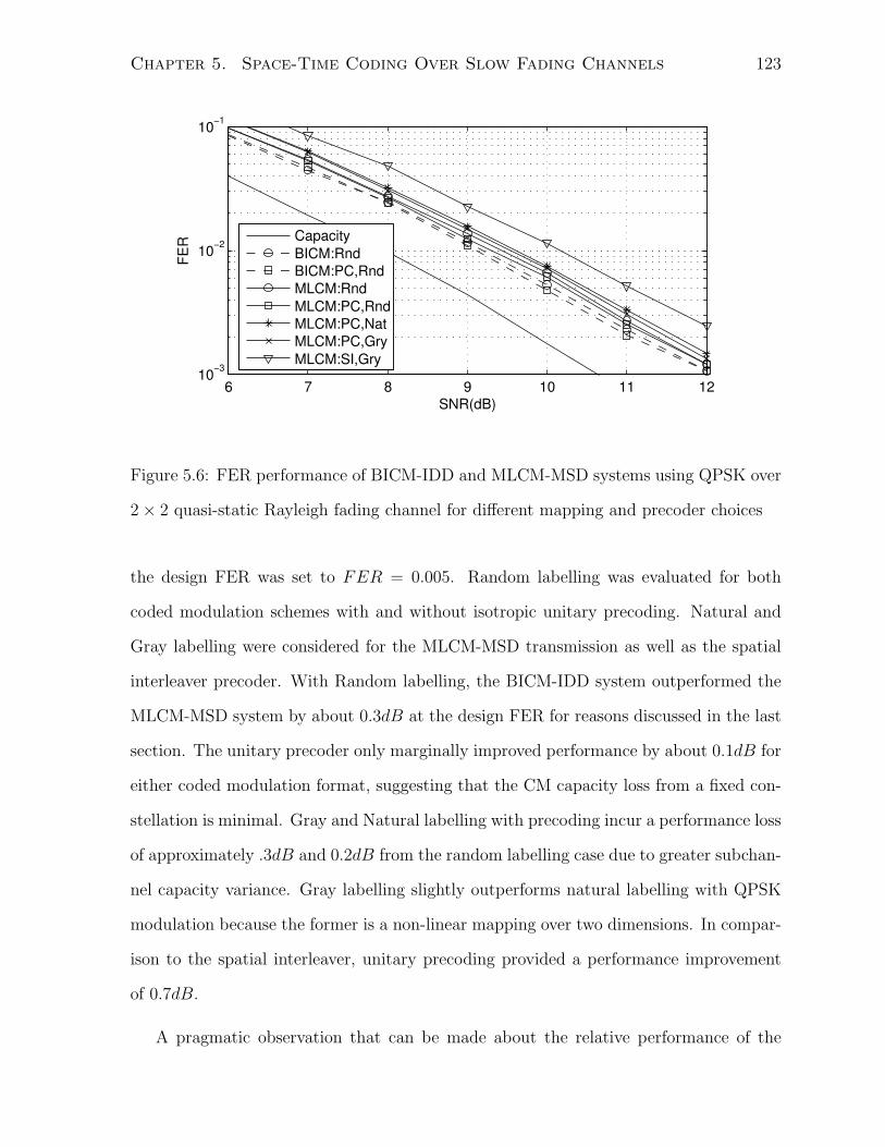
Chapter 5. Space-Time Coding Over Slow Fading Channels 123
6 7 8 9 10 11 1210−3
10−2
10−1
SNR(dB)
FER Capacity
BICM:RndBICM:PC,RndMLCM:RndMLCM:PC,RndMLCM:PC,NatMLCM:PC,GryMLCM:SI,Gry
Figure 5.6: FER performance of BICM-IDD and MLCM-MSD systems using QPSK over
2× 2 quasi-static Rayleigh fading channel for different mapping and precoder choices
the design FER was set to FER = 0.005. Random labelling was evaluated for both
coded modulation schemes with and without isotropic unitary precoding. Natural and
Gray labelling were considered for the MLCM-MSD transmission as well as the spatial
interleaver precoder. With Random labelling, the BICM-IDD system outperformed the
MLCM-MSD system by about 0.3dB at the design FER for reasons discussed in the last
section. The unitary precoder only marginally improved performance by about 0.1dB for
either coded modulation format, suggesting that the CM capacity loss from a fixed con-
stellation is minimal. Gray and Natural labelling with precoding incur a performance loss
of approximately .3dB and 0.2dB from the random labelling case due to greater subchan-
nel capacity variance. Gray labelling slightly outperforms natural labelling with QPSK
modulation because the former is a non-linear mapping over two dimensions. In compar-
ison to the spatial interleaver, unitary precoding provided a performance improvement
of 0.7dB.
A pragmatic observation that can be made about the relative performance of the
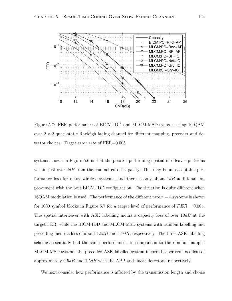
Chapter 5. Space-Time Coding Over Slow Fading Channels 124
10 12 14 16 18 20 22 24 26
10−3
10−2
10−1
SNR(dB)
FER
CapacityBICM:PC−Rnd−APMLCM:PC−Rnd−APMLCM:PC−SP−APMLCM:PC−SP−ICMLCM:PC−Nat−ICMLCM:PC−Gry−ICMLCM:SI−Gry−IC
Figure 5.7: FER performance of BICM-IDD and MLCM-MSD systems using 16-QAM
over 2 × 2 quasi-static Rayleigh fading channel for different mapping, precoder and de-
tector choices. Target error rate of FER=0.005
systems shown in Figure 5.6 is that the poorest performing spatial interleaver performs
within just over 2dB from the channel cutoff capacity. This may be an acceptable per-
formance loss for many wireless systems, and there is only about 1dB additional im-
provement with the best BICM-IDD configuration. The situation is quite different when
16QAM modulation is used. The performance of the different rate r = 4 systems is shown
for 1000 symbol blocks in Figure 5.7 for a target level of performance of FER = 0.005.
The spatial interleaver with ASK labelling incurs a capacity loss of over 10dB at the
target FER, while the BICM-IDD and MLCM-MSD systems with random labelling and
precoding incurs a loss of about 1.5dB and 1.9dB, respectively. The three ASK labelling
schemes essentially had the same performance. In comparison to the random mapped
MLCM-MSD system, the precoded ASK labelled system incurred a performance loss of
approximately 0.5dB and 1.5dB with the APP and linear detectors, respectively.
We next consider how performance is affected by the transmission length and choice
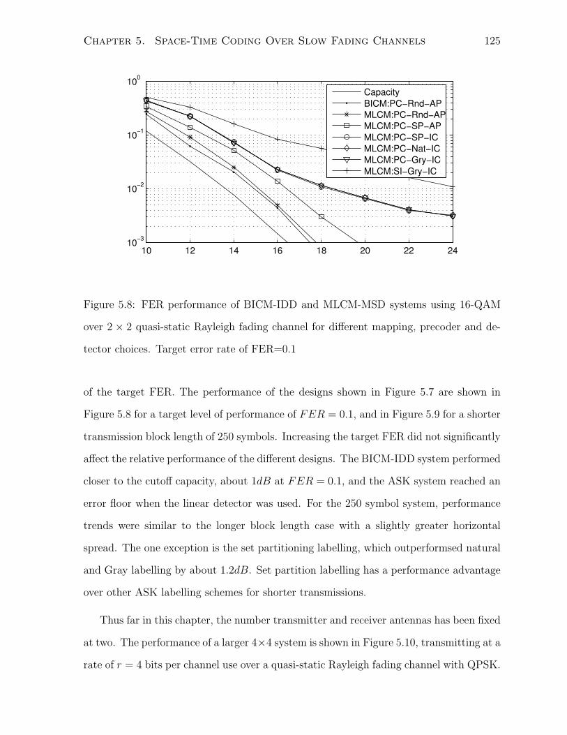
Chapter 5. Space-Time Coding Over Slow Fading Channels 125
10 12 14 16 18 20 22 2410−3
10−2
10−1
100
CapacityBICM:PC−Rnd−APMLCM:PC−Rnd−APMLCM:PC−SP−APMLCM:PC−SP−ICMLCM:PC−Nat−ICMLCM:PC−Gry−ICMLCM:SI−Gry−IC
Figure 5.8: FER performance of BICM-IDD and MLCM-MSD systems using 16-QAM
over 2 × 2 quasi-static Rayleigh fading channel for different mapping, precoder and de-
tector choices. Target error rate of FER=0.1
of the target FER. The performance of the designs shown in Figure 5.7 are shown in
Figure 5.8 for a target level of performance of FER = 0.1, and in Figure 5.9 for a shorter
transmission block length of 250 symbols. Increasing the target FER did not significantly
affect the relative performance of the different designs. The BICM-IDD system performed
closer to the cutoff capacity, about 1dB at FER = 0.1, and the ASK system reached an
error floor when the linear detector was used. For the 250 symbol system, performance
trends were similar to the longer block length case with a slightly greater horizontal
spread. The one exception is the set partitioning labelling, which outperformsed natural
and Gray labelling by about 1.2dB. Set partition labelling has a performance advantage
over other ASK labelling schemes for shorter transmissions.
Thus far in this chapter, the number transmitter and receiver antennas has been fixed
at two. The performance of a larger 4×4 system is shown in Figure 5.10, transmitting at a
rate of r = 4 bits per channel use over a quasi-static Rayleigh fading channel with QPSK.

Chapter 5. Space-Time Coding Over Slow Fading Channels 126
10 12 14 16 18 20 22 24 26
10−3
10−2
10−1
100
SNR(dB)
FER
CapacityBICM:PC−Rnd−APMLCM:PC−Rnd−APMLCM:PC−SP−APMLCM:PC−SP−ICMLCM:PC−Nat−ICMLCM:PC−Gry−ICMLCM:SI−Gry−IC
Figure 5.9: FER performance of BICM-IDD and MLCM-MSD systems using 16-QAM
over 2 × 2 quasi-static Rayleigh fading channel for different mapping, precoder and de-
tector choices and block size Ns = 250.
When random labelling was used, precoding did not measurably affect performance for
either coded modulation format, indicating that a fixed constellation has minimal effect
on the CM capacity for larger antenna systems. With random labelling, the BICM-IDD
system performed about 1dB from the cutoff capacity and the MLCM-MSD system in-
curred an additional 0.4dB loss. Gray and Natural labelling had approximately the same
performance that was 0.4dB and 0.8dB worse than the random labelling case for the APP
and linear detectors, respectively. Since the Gray mapped QPSK constellation is a non-
linear mapping over two complex dimensions, the linear detector was implemented as a
group detector over two dimensions. Finally, the precoder provided 0.25dB improvement
over the spatial interleaver.
Going to the higher rate 16-QAM modulation gives rise to certain computational
complexity issues in the 4×4 system, since it is difficult to use the APP detector in Monte
Carlo simulations. It follows that random labelling with APP detection is likely too
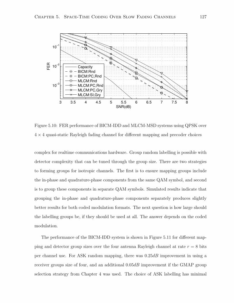
Chapter 5. Space-Time Coding Over Slow Fading Channels 127
3 3.5 4 4.5 5 5.5 6 6.5 7 7.5 8
10−3
10−2
10−1
SNR(dB)
FER
CapacityBICM:RndBICM:PC,RndMLCM:RndMLCM:PC,RndMLCM:PC,GryMLCM:SI,Gry
Figure 5.10: FER performance of BICM-IDD and MLCM-MSD systems using QPSK over
4× 4 quasi-static Rayleigh fading channel for different mapping and precoder choices
complex for realtime communications hardware. Group random labelling is possible with
detector complexity that can be tuned through the group size. There are two strategies
to forming groups for isotropic channels. The first is to ensure mapping groups include
the in-phase and quadrature-phase components from the same QAM symbol, and second
is to group these components in separate QAM symbols. Simulated results indicate that
grouping the in-phase and quadrature-phase components separately produces slightly
better results for both coded modulation formats. The next question is how large should
the labelling groups be, if they should be used at all. The answer depends on the coded
modulation.
The performance of the BICM-IDD system is shown in Figure 5.11 for different map-
ping and detector group sizes over the four antenna Rayleigh channel at rate r = 8 bits
per channel use. For ASK random mapping, there was 0.25dB improvement in using a
receiver groups size of four, and an additional 0.05dB improvement if the GMAP group
selection strategy from Chapter 4 was used. The choice of ASK labelling has minimal

Chapter 5. Space-Time Coding Over Slow Fading Channels 128
9 10 11 12 13 14 15
10−3
10−2
10−1
CapacityRnd1,GS=1Rnd4,GS=4Rnd1,GS=4Rnd1,GS=4,GSelRnd2,GS=4,GSel
Figure 5.11: FER performance of BICM-IDD system using 16-QAM over 4 × 4 quasi-
static Rayleigh fading channel for different mapping, and detector choices, and block size
Ns = 1000.
impact on performance in this system, and random ASK labelling was used for consis-
tency with other cases. For a fixed detector group size, increasing the label group size
actually degrades performance. For a detector groups size of GS = 4, the ASK ran-
dom labelling system outperformed the size two and four random labelled systems by
0.3dB and 0.7dB, respectively. The situation is different for the MLCM systems whose
performance is shown in Figure 5.12. Random labelling over four dimensions outper-
formed set partitioning by 0.25dB and 0.5dB for a detector group sizes of GS = 4 and
GS = 1, respectively. Set partitioning labelling had the best performance of the ASK
mapping schemes considered. Finally, unitary precoding provided a 0.9dB performance
improvement over spatial interleaving for Gray labelling, and approximately the same
improvement over other ASK labelling schemes, although the results are not shown.
The performance trends of the BICM-IDD and MLCM-MSD systems over the 4× 4
channel are affected by the transmission block length. The best BICM-IDD and MLCM-

Chapter 5. Space-Time Coding Over Slow Fading Channels 129
9 10 11 12 13 14 15
10−3
10−2
10−1
SNR(dB)
FER
CapacityPC,Rnd4,GS=4PC,SP,GS=4PC,SP,GS=1SI,Gry,GS=1
Figure 5.12: FER performance of MLCM-MSD system using 16-QAM over 4× 4 quasi-
static Rayleigh fading channel for different mapping, precoder and detector choices, and
block size Ns = 1000.
MSD systems both performed about 2dB from the cutoff capacity, with the BICM-IDD
system doing slightly better for a transmission length of 1000 symbols. Shortening the
block size to 250 symbols gives the BICM-IDD system a 1dB performance gain over
comparable MLCM-MSD configurations. It is some what surprising that the GMAP
group selection was outperformed by the fixed detector groupings in the BICM-IDD
system. The reason for this is that group selection strategies introduce more detector
message correlation, and this becomes a critical factor for the shorter block lengths. For
the MLCM configuration, set partitioning with linear detection performed particularly
well, 0.5dB worse than the group random mapped system.
In many wireless applications, there may be a different number of transmitter and
receiver antennas. Systems with more receiver antennas are easy to equalize, while it
has been argued in Chapter 4 that the detector is a key design element in the overloaded
scenario with a greater number of transmitter antennas. The performance of different
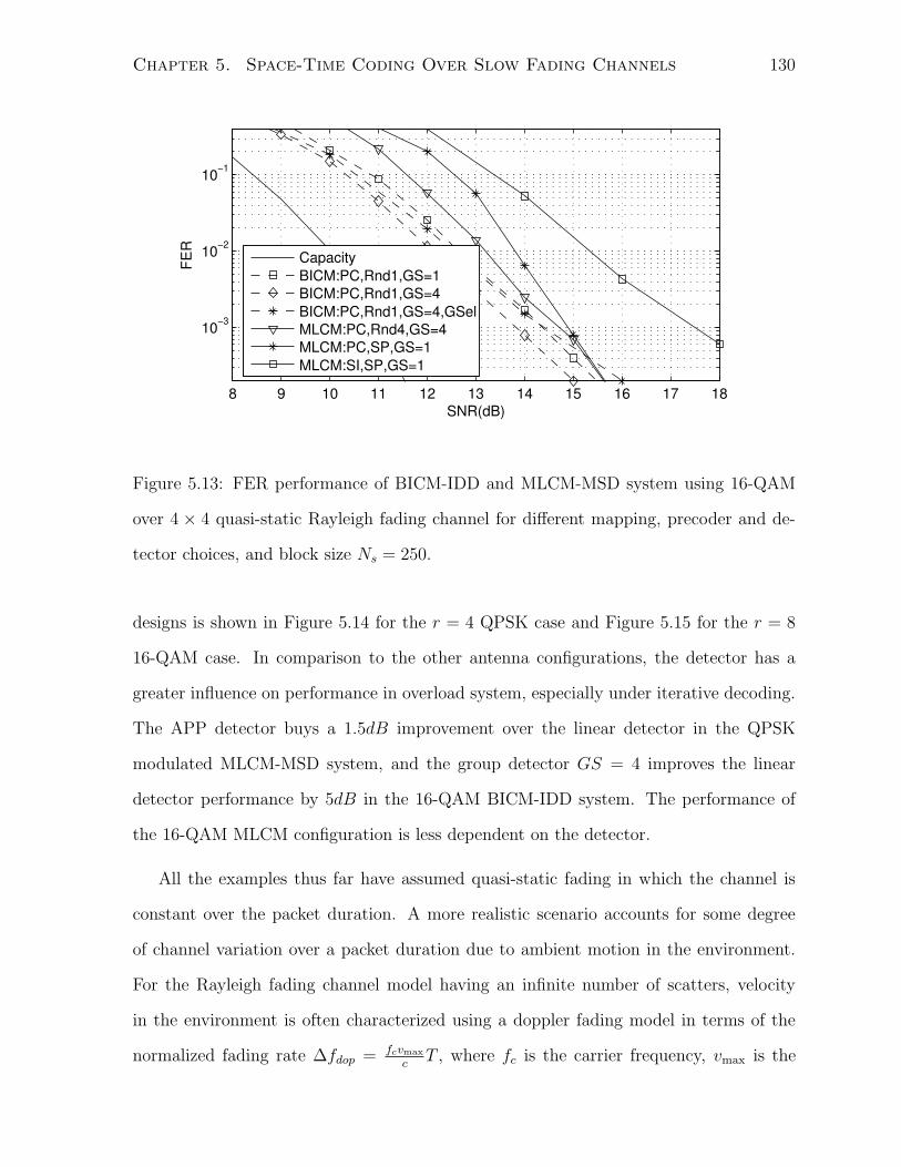
Chapter 5. Space-Time Coding Over Slow Fading Channels 130
8 9 10 11 12 13 14 15 16 17 18
10−3
10−2
10−1
SNR(dB)
FER
CapacityBICM:PC,Rnd1,GS=1BICM:PC,Rnd1,GS=4BICM:PC,Rnd1,GS=4,GSelMLCM:PC,Rnd4,GS=4MLCM:PC,SP,GS=1MLCM:SI,SP,GS=1
Figure 5.13: FER performance of BICM-IDD and MLCM-MSD system using 16-QAM
over 4 × 4 quasi-static Rayleigh fading channel for different mapping, precoder and de-
tector choices, and block size Ns = 250.
designs is shown in Figure 5.14 for the r = 4 QPSK case and Figure 5.15 for the r = 8
16-QAM case. In comparison to the other antenna configurations, the detector has a
greater influence on performance in overload system, especially under iterative decoding.
The APP detector buys a 1.5dB improvement over the linear detector in the QPSK
modulated MLCM-MSD system, and the group detector GS = 4 improves the linear
detector performance by 5dB in the 16-QAM BICM-IDD system. The performance of
the 16-QAM MLCM configuration is less dependent on the detector.
All the examples thus far have assumed quasi-static fading in which the channel is
constant over the packet duration. A more realistic scenario accounts for some degree
of channel variation over a packet duration due to ambient motion in the environment.
For the Rayleigh fading channel model having an infinite number of scatters, velocity
in the environment is often characterized using a doppler fading model in terms of the
normalized fading rate ∆fdop = fcvmax
cT , where fc is the carrier frequency, vmax is the
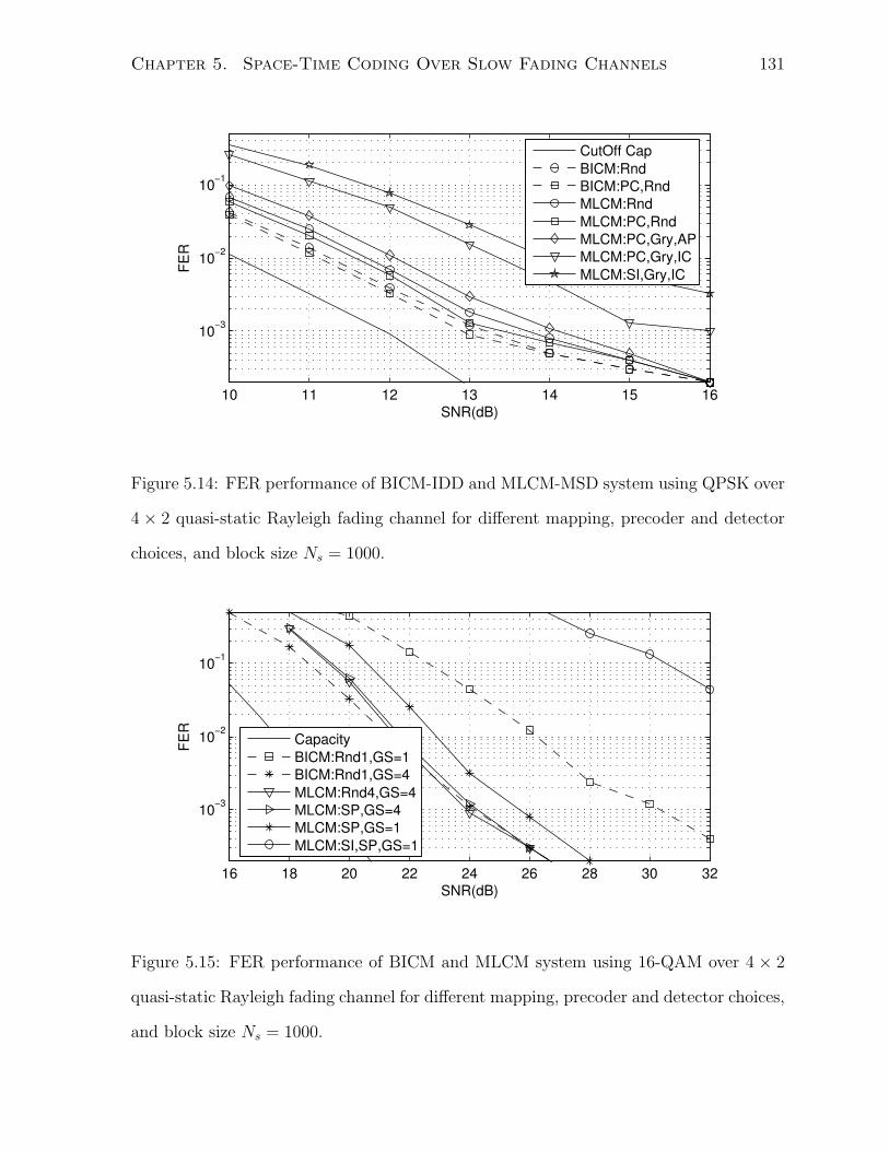
Chapter 5. Space-Time Coding Over Slow Fading Channels 131
10 11 12 13 14 15 16
10−3
10−2
10−1
SNR(dB)
FER
CutOff CapBICM:RndBICM:PC,RndMLCM:RndMLCM:PC,RndMLCM:PC,Gry,APMLCM:PC,Gry,ICMLCM:SI,Gry,IC
Figure 5.14: FER performance of BICM-IDD and MLCM-MSD system using QPSK over
4 × 2 quasi-static Rayleigh fading channel for different mapping, precoder and detector
choices, and block size Ns = 1000.
16 18 20 22 24 26 28 30 32
10−3
10−2
10−1
SNR(dB)
FER
CapacityBICM:Rnd1,GS=1BICM:Rnd1,GS=4MLCM:Rnd4,GS=4MLCM:SP,GS=4MLCM:SP,GS=1MLCM:SI,SP,GS=1
Figure 5.15: FER performance of BICM and MLCM system using 16-QAM over 4 × 2
quasi-static Rayleigh fading channel for different mapping, precoder and detector choices,
and block size Ns = 1000.

Chapter 5. Space-Time Coding Over Slow Fading Channels 132
maximum velocity and c is the speed of light, and T is the symbol time. In an effort
to find a working upper bound on ∆fdop, consider choosing parameter value fc = 5Ghz,
vmax = 120km/h and fs = 1/T = 50kHz. Higher carrier frequencies tend to require a
line-of-sight component, the velocity is limited by local driving speeding limits, and the
spectral bandwidth is chosen in light of transmission bandwidth and latency demands in
next generation systems. These parameter values give a normalized fading rate of about
∆fdop = 0.01. Choosing a normalized fading rate much higher may start to undermine
assumptions of perfect receiver CSI and negligible ISI due to the doppler spread in the
combined channel and pulse shaping filter response.
The performance of the various BICM-IDD and MLCM-MSD systems is shown for
the 2 × 2 doppler Rayleigh fading channel in Figure 5.16 for packets of 1000 symbols,
and in Figure 5.17 for packets of 250 symbols. A normalized fading rate of ∆fdop = 0.01
and design rate of r = 4 was used. An independent Rayleigh fading spatial model
was used with time correlation generated through a modified Jake’s model [132]. One
may observe that the channel cutoff capacity is roughly 2dB farther to the right in
the 250 symbol systems. This is because as the transmission window expands to infinity,
channel statistics become stationary and performance approaches the independent fading
scenario. Other performance trends were similar to previously discussed systems.
The final set of simulations examine different spatial fading phenomena. The Rayleigh
fading model is based on an infinite set of isotropic scatter with no line-of-sight compo-
nent or antenna correlation. The performance of the different systems is shown for the
2× 2 Rican channel with k-factor kRic = 1 in Figure 5.18. The performance is shown for
the correlated Rayleigh fading channel in Figure 5.19, with a transmitter and receiver an-
tenna correlation coefficient of α = 0.5. In comparison to the Rayleigh channel, antenna
correlation reduces performance and the line-of-sight component improves performance
at the same SNR. The BICM-IDD and MLCM-MSD code parameters were designed for
both the actual spatial fading model as well as the generic Rayleigh fading model. Code

Chapter 5. Space-Time Coding Over Slow Fading Channels 133
6 6.5 7 7.5 8 8.5 9 9.5 10 10.5
10−3
10−2
10−1
SNR(dB)
FER
CapacityBICM:PC,Rnd,APMLCM:PC,Rnd,APMLCM:PC,SP,APMLCM:PC,SP,ICMLCM:SI,SP,IC
Figure 5.16: FER performance of BICM-IDD and MLCM-MSD system using 16-QAM
over 2 × 2 doppler Rayleigh fading channel with ∆fdop = 0.01 for different mapping,
precoder and detector choices, and block size Ns = 1000.
7 8 9 10 11 12 13 14 15
10−3
10−2
10−1
SNR(dB)
FER
CapacityBICM:PC,Rnd,APMLCM:PC,Rnd,APMLCM:PC,SP,APMLCM:PC,SP,ICMLCM:SI,SP,IC
Figure 5.17: FER performance of BICM-IDD and MLCM-MSD system using 16-QAM
over 2 × 2 doppler Rayleigh fading channel with ∆fdop = 0.01 for different mapping,
precoder and detector choices, and block size Ns = 250.
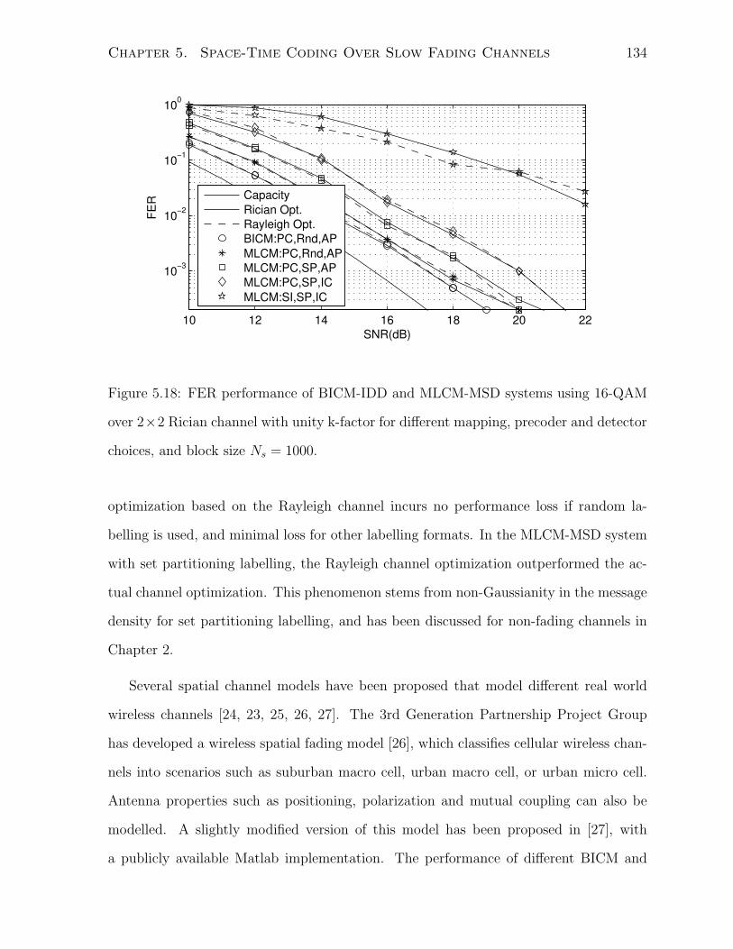
Chapter 5. Space-Time Coding Over Slow Fading Channels 134
10 12 14 16 18 20 22
10−3
10−2
10−1
100
SNR(dB)
FER Capacity
Rician Opt.Rayleigh Opt.BICM:PC,Rnd,APMLCM:PC,Rnd,APMLCM:PC,SP,APMLCM:PC,SP,ICMLCM:SI,SP,IC
Figure 5.18: FER performance of BICM-IDD and MLCM-MSD systems using 16-QAM
over 2×2 Rician channel with unity k-factor for different mapping, precoder and detector
choices, and block size Ns = 1000.
optimization based on the Rayleigh channel incurs no performance loss if random la-
belling is used, and minimal loss for other labelling formats. In the MLCM-MSD system
with set partitioning labelling, the Rayleigh channel optimization outperformed the ac-
tual channel optimization. This phenomenon stems from non-Gaussianity in the message
density for set partitioning labelling, and has been discussed for non-fading channels in
Chapter 2.
Several spatial channel models have been proposed that model different real world
wireless channels [24, 23, 25, 26, 27]. The 3rd Generation Partnership Project Group
has developed a wireless spatial fading model [26], which classifies cellular wireless chan-
nels into scenarios such as suburban macro cell, urban macro cell, or urban micro cell.
Antenna properties such as positioning, polarization and mutual coupling can also be
modelled. A slightly modified version of this model has been proposed in [27], with
a publicly available Matlab implementation. The performance of different BICM and

Chapter 5. Space-Time Coding Over Slow Fading Channels 135
10 12 14 16 18 20 22 24 26
10−3
10−2
10−1
100
SNR(dB)
FER Capacity
RayCorr Opt.Rayleigh Opt.BICM:PC,Rnd,APMLCM:PC,Rnd,APMLCM:PC,SP,APMLCM:PC,SP,ICMLCM:SI,SP,IC
Figure 5.19: FER performance of BICM-IDD and MLCM-MSD systems using 16-QAM
over 2 × 2 correlated Rayleigh fading channel (α = 0.5) for different mapping, precoder
and detector choices, and block size Ns = 1000.
MLCM systems has been evaluated using the model from [27]. The set of default param-
eters from [27] was used, except that the symbol frequency was set to fs = 400kHz. At
this symbol rate, the urban macro cell environment gives rise to non-negligible ISI due
to multipath and will not be considered. Any residual ISI due to multipath for the other
two environments is omitted.
The performance of different BICM-IDD and MLCM-MSD designs is shown for the
urban microcell environment in Figure 5.20 and for the suburban macrocell environment
in Figure 5.21. Both environments have a lower capacity than the Rayleigh fading channel
at the same SNR. For the urban microcell environment, the code optimizations for the
Rayleigh and actual channel models produced similar results for the cases considered. For
the suburban environment, the Rayleigh and actual channel model produced essentially
identical results for the BICM-IDD system, but the Rayleigh optimization performed
worse in the MLCM-MSD system. The performance loss in the MLCM-MSD Rayleigh
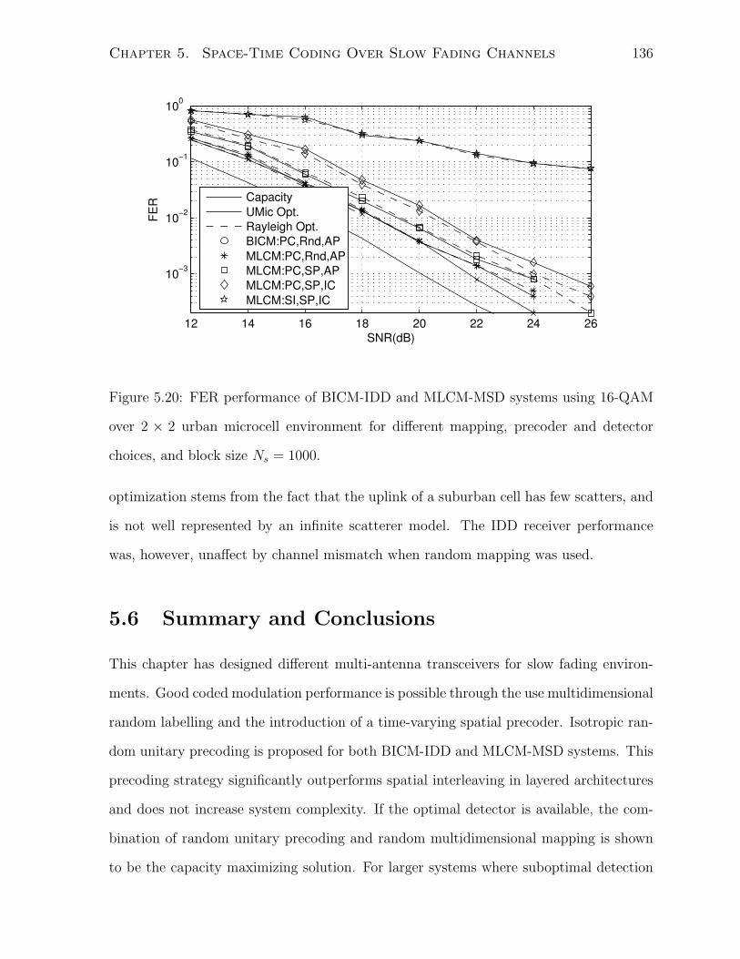
Chapter 5. Space-Time Coding Over Slow Fading Channels 136
12 14 16 18 20 22 24 26
10−3
10−2
10−1
100
SNR(dB)
FER Capacity
UMic Opt.Rayleigh Opt.BICM:PC,Rnd,APMLCM:PC,Rnd,APMLCM:PC,SP,APMLCM:PC,SP,ICMLCM:SI,SP,IC
Figure 5.20: FER performance of BICM-IDD and MLCM-MSD systems using 16-QAM
over 2 × 2 urban microcell environment for different mapping, precoder and detector
choices, and block size Ns = 1000.
optimization stems from the fact that the uplink of a suburban cell has few scatters, and
is not well represented by an infinite scatterer model. The IDD receiver performance
was, however, unaffect by channel mismatch when random mapping was used.
5.6 Summary and Conclusions
This chapter has designed different multi-antenna transceivers for slow fading environ-
ments. Good coded modulation performance is possible through the use multidimensional
random labelling and the introduction of a time-varying spatial precoder. Isotropic ran-
dom unitary precoding is proposed for both BICM-IDD and MLCM-MSD systems. This
precoding strategy significantly outperforms spatial interleaving in layered architectures
and does not increase system complexity. If the optimal detector is available, the com-
bination of random unitary precoding and random multidimensional mapping is shown
to be the capacity maximizing solution. For larger systems where suboptimal detection
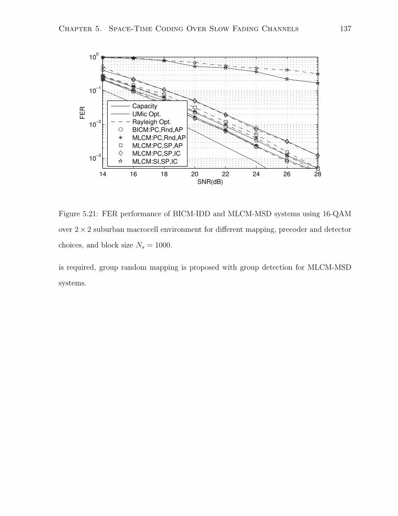
Chapter 5. Space-Time Coding Over Slow Fading Channels 137
14 16 18 20 22 24 26 28
10−3
10−2
10−1
100
SNR(dB)
FER Capacity
UMic Opt.Rayleigh Opt.BICM:PC,Rnd,APMLCM:PC,Rnd,APMLCM:PC,SP,APMLCM:PC,SP,ICMLCM:SI,SP,IC
Figure 5.21: FER performance of BICM-IDD and MLCM-MSD systems using 16-QAM
over 2× 2 suburban macrocell environment for different mapping, precoder and detector
choices, and block size Ns = 1000.
is required, group random mapping is proposed with group detection for MLCM-MSD
systems.
Chapter 6
Summary and Conclusions
This dissertation has analyzed the design of a single-carrier multi-antenna wireless system
under slow-fading conditions. Multi-antenna systems hold great capacity gains in a
highly scattered environment that are exploited through an appropriate design coded
modulation scheme and receiver structure. Novel contributions are made in serval aspects
of space-time transceiver design.
6.1 Key Contributions
Under slow and quasi-static fading conditions, coded modulation performance depends
largely on precoder and mapper design. Random isotropic unitary precoding is proposed
for both MLCM and BICM transmissions. Random precoding allows the use of a low
complexity MMSE detector, and provides significant performance gains over spatially
interleaving in MLCM-MSD systems. When the APP detector is available, a strat-
egy of applying both random unitary precoding and random multidimensional mapping
maximizes fading performance in both BICM-IDD and MLCM-MSD systems. Although
multidimensional random labelling in MLCM-MSD transmissions has been discussed else-
where, their use in BICM-IDD transmissions to combat slow fading is unique, to the best
of our knowledge. We also show that under quasi-static fading conditions, the BICM-
138
Chapter 6. Summary and Conclusions 139
IDD structure has a performance advantage over the MLCM-MSD structure, even for
long packet transmissions.
The problem of multi-antenna detection has been examined in high dimensional sys-
tems where the optimal detector is computational infeasible. Two detectors based on a
group detection strategy have been proposed for either MSD or IDD receivers. These
detectors bridge the performance/complexity gap between the MMSE and APP detec-
tors. For MLCM-MSD transmissions, group detection is combined with group random
labelling yielding improved performance. The work on group detection in Chapter 4 has
been published in [96, 97, 98].
Coded modulation design using LDPC codes has been considered for BICM-IDD and
MLCM-MSD structures. MLCM-MSD transmissions require subcodes to be design over
a wide range of rates when capacity efficient mapping functions are used. A generalized
LDPC code structure has been proposed that improves the low-rate performance of con-
ventional LDPC codes. The check node is generalized by adding additional check node
parity bit that are connected directly to the channel. This reduces the rate of the LDPC
subcode, leading a performance gain in the low rate R < 1/3 region. In MLCM-MSD
transmissions, the proposed generalized LDPC codes outperform conventional LDPC
code construction over a wide range of transmission rates and channels.
Concatenated convolutional codes are another class of widely used binary codes in
coded modulation applications. A convolutional code can be made irregular by encoding
fractions of bits with different puncture patterns and mother codes of different memory.
Fixed size and variable size trellis have been proposed to connected different memory
mother codes. In multi-antenna BICM-IDD transmissions, irregular convolutional codes
outperform comparable turbo coded and GLDPC coded systems.

Chapter 6. Summary and Conclusions 140
6.2 Future Directions
The future directions of this dissertation can be divided into two broad categories. The
first relates to improvements in the analysis procedures and component design that would
improve over-all system performance. The second category stems from expanding the
application scope beyond a single-carrier single-user system transmitting an uncorrelated
binary data source.
6.2.1 Methods
There are a number of possible improvements to the analysis and design procedures
discussed in this work. Some of these advancements are outlined as follows:
1. The analysis of iterative message passing through EXIT chart is central to the
work in this dissertation. One limitation of EXIT chart analysis is the assumption
that the message densities are Gaussian, which greatly simplifies the analysis. The
Gaussian assumption leads to certain performance limitations. For example, ex-
periments were conducted with parallel concatenated irregular convolutional codes,
but the non-Gaussian message density of the irregular code profile led to a mis-
match between the actual and predicted code threshold values. One way to improve
the accuracy of the EXIT chart design procedure is to use the EXIT chart decod-
ing trajectory in the analysis [133, 134]. If a convergence failure is consistently
observed at some early point, then an additional gap can be imposed between the
two EXIT curves in the affected region. This strategy was applied to some extent in
this work to mitigate error floor problems, although not in any systematic manner.
Another way to improve the accuracy of the EXIT chart analysis to assume the
message density takes on a parametric distribution. For LDPC codes, EXIT charts
have been developed using mix-Gaussian message densities [135] and through finite
order moment generation functions [136].
Chapter 6. Summary and Conclusions 141
A second major limitation of EXIT charts analysis is the assumption of uncorre-
lated message densities. Message correlations is particularly problematic for short
block length transmissions, making the EXIT chart prediction inaccurate. In this
dissertation, the effects of message correlation could only be assessed though brute
force Monte Carlo simulations. A systematic analysis of correlation from code,
mapper and interleaver components may lead to an improved EXIT model and
better overall system performance. Interleaver design has not been considered in
this work, and the problem of interleaver design with irregular codes and with IDD
processing is worth further study.
2. The generalized LDPC and irregular convolutional codes developed in the dis-
sertation are based on binary component codes. Non-binary convolutional turbo
codes [137] and LDPC codes [138] have been developed, with better performance
than their binary counter parts for the same block length. Non-binary subcodes
can also offer more degrees of freedom in designing an irregular code profile.
3. Modulation has not been a primary focus of this dissertation, as only QAM mod-
ulation formats have been considered. One limitation of QAM modulation is that
for equiprobable constellation points, there is a capacity loss in the low rate re-
gion. This is a large part of the reason why in Chapter 2, the rate r = 1 16-QAM
GLDPC coded BICM-IDD system did not outperform a comparable QPSK mod-
ulated system. QAM modulation formats with irregular level spacing have been
proposed [139], leading to a constellation shaping gain for the AWGN channel.
This modulation strategy may expand the use of proposed GLDPC codes in low-
rate BICM-IDD applications.
Another problem that is related to modulation is the appearance of zero-rate sub-
codes in MLCM transmissions. In Chapter 5, the 4 × 2 16-QAM MLCM-MSD
system with group random labelling had two zero-rate subcodes encoded with a

Chapter 6. Summary and Conclusions 142
pseudo-random sequence. There were also other cases of zero-rate subcode. One
strategy to avoid zero-rate subcodes is to use an irregular modulation scheme that
consists of an aggregate of QPSK and 16-QAM symbols on different antenna. This
would facilitate greater control of the subcode rate distribution so that zero-rate
subcodes could be avoided.
6.2.2 Applications
By expanding the scope of application of this research, there are a number of possible
directions of future study that may lead useful designs. Some of these applications are
described as follows:
1. Multimedia applications are a major driving force behind high-bandwidth commu-
nication systems. Treating image and video stream data as an uncorrelated binary
data source, may not address end-to-end system goals. For example, an image
may be divided into different layers, where course and fine image data are mapped
to different layers with different levels of protection. Much of the work herein on
MLCM-MSD transmissions can be extend to applications involving unequal error
protection. Another consideration is how source and channel coding should be ap-
plied together, since their separation is only optimal for long bursts over stationary
ergodic channel. Shorter packets and slow-fading conditions lead to additional gain
from joint source-channel encoding and decoding structures. Some of the work
herein on IDD and MSD receiver processing can be expanded to include source
decoding.
2. This work has only considered single-carrier transmissions, although multi-carrier
modulation is a part of current and next generation wireless networking and cel-
lular standards. OFDM divides a frequency selective channel into a set of parallel
frequency-flat channels. The correlation between two channels is a function of the

Chapter 6. Summary and Conclusions 143
frequency spacing between them, thus tones with sufficient frequency separation
undergo approximately independent fading. A virtual MIMO channel can be con-
structed over independently fading OFDM tones instead of over multiple antennas,
which would produce a block diagonal channel matrix. Over quasi-static and slow
fading channels using OFDM, the unitary precoding and multidimensional map-
ping strategies of Chapter 5 can be applied across tones. One would expect similar
performance improvements at the cost of increase detector complexity.
3. The work herein is limited to a simple single-user point-to-point communications
systems. More realistic wireless networks have several users that share the physical
channel or access to it. Current multiuser systems are either based on OFDM
multiple access or Code Division Multiple Access (CDMA). MIMO CDMA may
hold some interest developments, as there are many parallels between multi-user
and spatially multiplexed systems. Layered architecture have been combined with
CDMA spreading codes [106] with group detection [106] over the uplink channel.
There is also a similarity between random chip sequences, random precoding and
random mapping that is worth some investigations.
Another interesting scenario is where there are several network nodes cooperate to
enhance the transmission rate and reliability. Through cooperative coding [140],
higher throughput is possible by exploiting the additional spatial diversity of multi-
ple wireless links. There are a number of coding and media access control strategies
that maybe applied to increase transmission rate. Some possible physical layer de-
signs may include group detection and spatial coding strategies similar to those
discussing in this dissertation.
Appendix A
Appendix
A.1 Relationship between RDMAP/GMAP detec-
tors and MAP/MMSE detector
In this appendix, lemmas 4.1, 4.2 from Chapter 4 are proven showing that the RDMAP/GMAP
detector is a generalization of both the MAP detector and MMSE detector in [116, 117].
lemma 4.1: The RDMAP detector and MAP detector are equivalent for NG = 2N .
proof: For NG = 2N , sG = Ps and HG = HPT , where P is a permutation matrix.
Also, w = v is a zero mean Gaussian scaler that has a whitening filter vector F = 1/σ2.
The RDMAP decision in (4.10) for a bit bi corresponds to a symbol si = sGj that can be
expressed as
Λ1[bi] = log
∑
sG∈SG,sGj=+1 P (sG) exp(
−‖σ−1r−σ−1HPT Ps‖2
2
)
∑
sG∈SG,sGj=−1 P (sG) exp(
−‖σ−1r−σ−1HPT Ps‖2
2
) (A.1)
= log
∑
s∈S,si=+1 P (s) exp(
−‖r−Hs‖2
2σ2
)
∑
s∈S,si=−1 P (s) exp(
−‖r−Hs‖2
2σ2
) (A.2)
which is the MAP decision rule in (4.5).
lemma 4.2: The RDMAP detector and MMSE detector in [116, 117] are equivalent
for NG = 1.
144

Appendix A. Appendix 145
proof: The MMSE detector in [116, 117] uses a combination of soft interference
cancellation and a MMSE residual suppression filter. To make a decision for a bit bi, the
channel observation after interference cancellation is given by
ri = r−Hsi (A.3)
where si = [s1, . . . , si−1, 0, si+1, . . . , sN ]T , sj = tanh(λp2[bj]/2), and QPSK is assumed.
The output ri is filtered with a residual MMSE filter given by wTi = 2hT
i R−1i r, with
Ri = [HΩiHT + σ2I], Ωi = diag(ω1, . . . , ωi−1, 1, ωi+1, ωN ) and ωj = E[|si− si|2] = 1− s2
i .
The filter output is approximated as a Gaussian distribution to produce an extrinsic LLR
given by
λ1[bi] =2hT
i R−1i ri
1− hTi R−1
i hi
(A.4)
For the case where NG = 1, the RDMAP decision in (4.10) can be simplified as
Λ[bi] = logP (si = +1)
P (si = −1)− ‖y − Fhi‖2
2+‖y + Fhi‖2
2(A.5)
= λp2[bi] + 2hT
i FTy (A.6)
where the second term in (A.6) is the extrinsic output that can be further simplified as
λ1[bi] = 2hTi FTF(r− w) = 2hT
i R−1w (r− w) (A.7)
What is now required to be shown is that (A.7) and (A.4) are equivalent. First note that
ri = r− w, as it can be readily seen that Hsi = HGsG. What remains is to show that
R−1w ≡ R−1
i (1− hTi R−1
i hi)−1 (A.8)
Substituting Rw = Ri + hihTi on the l.h.s. of (A.8) and using the matrix inversion
lemma 1 with A = Ri, B = −1 and X = hi gives the expression on the r.h.s of (A.8)
after some simplification.
1(A + XBXT )−1 = A
−1 −A−1
X(B−1 + XTA−1
X)−1X
TA−1
Appendix A. Appendix 146
A.2 Evaluation of Noise Correlation Eigenvalues
This appendix discusses several methods to evaluate the expectation of the ordered eigen-
values of the noise correlation matrix Σc from Chapter 4. A direct method to determine
Σc is through Monte Carlo simulations. Such a method can be, however, computationally
intensive. Alternatively, the eigenvalues of Σc can be expressed as
eig[Σc] = 2 E[W(M,NIc)] + diag[Iσ2] (A.9)
where W(m,n) is a complex Wishart matrix of the form W(m,n) = H(m,n)H(m,n)H
and H(m,n) is a m×n matrix of independent complex zero-mean Gaussian entries with
unity variance. The pdf of the ordered eigenvalues λ1 ≤ λ2 ≤ · · · ≤ λm of W(m,n) is
given by [141]
P (λ1, λ2, . . . , λm) =πm(m−1)
Γm(n)Γm(m)exp
[
m∑
i=1
λi
]
m∏
i=1
λn−mi
∏
i<j
(λi − λj)2 (A.10)
where Γm(a) = πm(m−1)/2∏m
i=1 Γ(a− i + 1) is the multivariate gamma function. The
expectation of the Wishart matrix eigenvalues can be directly evaluated by marginalizing
the joint pdf in (A.10). The number of factors on the right hand side of (A.10) grows
with m! and quickly becomes computationally infeasible for moderately large m. A
computationally more efficient method to find the expected eigenvalues can be adapted
from [119, appendix B]. This method exploits the intrinsic symmetry in eigenvalue pdf
and converts the m nested integrals (required to find the expectation) into m separate
integrals.
The method used in this appendix to find the expected eigenvalues of the Wishart
matrix is simpler than the methods previously discussed and it is based on the the
asymptotic eigenvalue distribution as n,m → ∞. Letting m,n increase without bound
such that m/n → β asymptotically, the empirical distribution of F (x) = P (λ < x) of
W(m,n)/n converges to the non-random limit defined by [141]
dF (x) =
√
(x− a(β))(b(β)− x)
2πβx+ δ(x)I(β > 0)(1− 1/β) (A.11)

Appendix A. Appendix 147
for β 6= 1 where a(β) = (1 −√
(β))2, b(β) = (1 +√
(β))2. In the case of β = 1, one
has dF (x) = (2π)−1((4 − x)/x)1/2 for 0 ≤ x ≤ 4. The expectation of the eigenvalues of
W(m,n) can be found from (A.11), by dividing the domain of dF (x) into m adjacent
regions, such that each region has the same area under dF (x). Each region can be
represented by its center of mass under dF (x), denoted xi, i = 1 . . . m for the ith region.
The xis can be easily found by numerical integrating (A.11). The expected eigenvalues of
W(m,n) can then be approximated as E[eig[W(m,n)]] ≈ ndiag[x1, . . . , xm]. The use of
(A.11) to approximate the eigenvalues of W(m,n) tends to be accurate even for small m,
especially when n ≥ m. For the simulated examples in Chapter 5, there was negligible
difference in the estimated BER whether the mean eigenvalue matrix Σc was determined
through Monte Carlo simulations or by using the asymptotic distribution in (A.11).
A.3 MLCM-MSD rate and EXIT curve optimization
over slow fading
This appendix describes a method to solve the MSD rate allocation problem in (5.10) and
EXIT chart curve matching problem in (5.16). Both of these problems can be expressed
as follows:
arg maxxi
∑
i
g(xi) s.t. fER(xi, ρ) ≤ PER, (A.12)
where g(xi) and fER(xi, ρ) are monotonically increasing functions. For the MLCM-
MSD rate optimization, xi are the subchannel rates and g(x) = x, and for the EXIT
chart optimization xi are points on the EXIT graph and g(x) = Ich∗E (x). For the EXIT
chart optimization, there is additional monotonic constraint g(xi) > g(xj) > 0 ∀ xi > xj
that can be omitted because the design EXIT curve is constrained by channel realization
EXIT curves that are monotonic. In order to solve A.12, one can use the fact that
g(xi) and fER(xi, ρ) are monotonically increasing functions. Increasing a value xl can
only increase the overall rate and possibly the constraint function, while reducing xi will
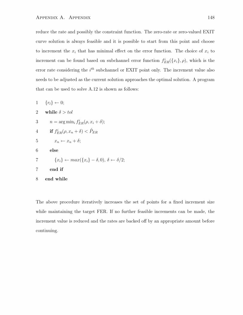
Appendix A. Appendix 148
reduce the rate and possibly the constraint function. The zero-rate or zero-valued EXIT
curve solution is always feasible and it is possible to start from this point and choose
to increment the xi that has minimal effect on the error function. The choice of xi to
increment can be found based on subchannel error function f iER(xi, ρ), which is the
error rate considering the ith subchannel or EXIT point only. The increment value also
needs to be adjusted as the current solution approaches the optimal solution. A program
that can be used to solve A.12 is shown as follows:
1 rl ← 0;
2 while δ > tol
3 n = arg mini fiER(ρ, xi + δ);
4 if f iER(ρ, xn + δ) < PER
5 xn ← xn + δ;
6 else
7 xi ← max(xi − δ, 0), δ ← δ/2;
7 end if
8 end while
The above procedure iteratively increases the set of points for a fixed increment size
while maintaining the target FER. If no further feasible increments can be made, the
increment value is reduced and the rates are backed off by an appropriate amount before
continuing.
Bibliography
[1] G. Foschini and M. Gans, “On limits of wireless communication in a fading enviorn-
ment when using multiple antennas,” Wireless Personal Communications, vol. 6,
pp. 311–335, 1998.
[2] I. Telatar, “Capacity of multi-antenna Gaussian channels,” European Transations
on Telecommunications, vol. 10, no. 6, pp. 585–595, 1999.
[3] G. Ungerboek, “Channel coding with multilevel/phase signals,” IEEE Transactions
on Information Theory, vol. 28, no. 1, pp. 55 – 67, Jan. 1982.
[4] ——, “8-psk trellis codes for a rayleigh channel,” IEEE Transactions on Commu-
nications, vol. 40, no. 1, pp. 873–884, Jan. 1992.
[5] G. Caire, Taricco, and E. Biglieri, “Bit-interleaved coded modulation,” IEEE
Transactions on Information Theory, vol. 44, no. 3, pp. 927–946, May 1998.
[6] A. Chindapol and J. Ritcey, “Design, analysis, and performance evaluation for
BICM-ID with square QAM constellations in Rayleigh fading channels,” IEEE
Journal on Selected Areas in Communications, vol. 5, no. 19, pp. 944 – 957, May
2001.
[7] H. Imai and S. Hirakawa, “A new multilevel coding method using error-correcting
codes,” IEEE Transactions on Information Theory, vol. 23, no. 3, pp. 371–377,
May 1977.
149
Bibliography 150
[8] U. Wachsmann, R. Fischer, and J. Huber, “Multilevel codes: theoretical concepts
and practical design rules,” IEEE Transactions on Communications, vol. 45, no. 5,
pp. 1361 – 1391, Jul. 1999.
[9] G. Foschini and M. Gans, “Layered space-time architecture for wireless communi-
cations in wireless fading environment when using multiple antennas,” Bell System
Technical Journal, vol. 1, no. 2, pp. 41–59, 1996.
[10] P. Robertson and T. Worz, “Bandwidth-efficient turbo trellis-coded modulation
using punctured component codes,” IEEE Journal on Selected Areas in Commu-
nications, vol. 16, no. 2, pp. 206 – 218, Feb. 1998.
[11] H. Holma, A. Toskala, K. Ranta-aho, and J. Pirskanen, “High-speed packet access
evolution in 3GPP release 7 [topics in radio communications],” IEEE Communica-
tions Magazine, vol. 45, no. 12, pp. 29 – 35, 2007.
[12] J. Gozalvez, “Ultra mobile broadband [mobile radio],” IEEE Vehicular Technology
Magazine, vol. 2, no. 1, pp. 51 – 55, 2007.
[13] C. Berrou, A. Glavieux, and P. Thitimajshima, “Near shannon limit error-
correcting coding and decoding: Turbo-codes,” in Proc. IEEE International Con-
ference Communications, May 1993, pp. 1064–1070.
[14] C. Berrou and A. Glavieux, “Near-optimum error-correcting coding and decoding:
Turbo codes,” IEEE Transactions on Communications, vol. 44, no. 10, p. 12611271,
Oct. 1996.
[15] R. Gallager, Low density parity check codes. Cambridge, MA: Ph.D dissertation,
Massachusetts Institute of Technology, 1960.
[16] D. MacKay, “Good error-correcting codes based on very sparse matrices,” IEEE
Transactions on Information Theory, vol. 45, no. 2, pp. 399 – 431, Mar. 1999.

Bibliography 151
[17] D. MacKay, S. Wilson, and M. Davey, “Comparison of constructions of irregular
Gallager codes,” IEEE Transactions on Communications, vol. 47, no. 10, pp. 1449
– 1454, Oct. 1999.
[18] T. Richardson, M. Shokrollahi, and R. Urbanke, “Design of capacity-approaching
irregular low-density parity-check codes,” IEEE Transactions on Information The-
ory, vol. 47, no. 2, pp. 619–637, Feb. 2001.
[19] S. ten Brink, “Convergence behavior of iteratively decoded parallel concatenated
codes,” IEEE Transactions on Communications, vol. 49, no. 10, pp. 1727 – 1737,
Oct. 2001.
[20] S. Brink, G. Kramer, and A. Ashikhmin, “Design of low-density parity-check codes
for modulation and detection,” IEEE Transactions on Communications, vol. 52,
no. 4, pp. 670 – 678, Apr. 2004.
[21] A. Ashikmin, G. Kramer, and S. ten Brink, “Extrinsic information transfer func-
tions: Model and erasure channel property,” IEEE Transactions on Information
Theory, vol. 50, no. 11, p. 2657 2673, Nov. 2004.
[22] J. Wallace and M. Jensen, “Modeling the indoor MIMO wireless channel,” IEEE
Transactions on Antennas and Propagation, vol. 50, no. 5, pp. 591 – 599, May 2002.
[23] W. Weichselberger, M. Herdin, H. Ozcelik, and E. Bonek, “A stochastic MIMO
channel model with joint correlation of both link ends,” IEEE Transactions on
Wireless Communications, vol. 5, no. 1, pp. 90 – 100, Jan. 2006.
[24] H. Shin and J. Lee, “Capacity of multiple-antenna fading channels: spatial fading
correlation, double scattering, and keyhole,” IEEE Transactions on Information
Theory, vol. 49, no. 10, pp. 2636 – 2647, Oct. 2003.
Bibliography 152
[25] T. Zwick, C. Fischer, and W. Wiesbeck, “A stochastic multipath channel model
including path directions for indoor environments,” IEEE Journal on Selected Areas
in Communications, vol. 20, no. 6, pp. 1178 – 1192, Aug. 2002.
[26] 3GPP, “Spatial channel model for multiple input multiple output (MIMO) simula-
tions,” TR 25.996 V6.1.0, Sep. 2003.
[27] J. Salo, G. Del Galdo, J. Salmi, P. Kysti, M. Milojevic, D. Laselva, and C. Schnei-
der. (2005, Jan.) MATLAB implementation of the 3GPP Spatial Channel Model
(3GPP TR 25.996). [Online]. Available: http://www.tkk.fi/Units/Radio/scm/
[28] G. Levin and S. Loyka, “Multi-keyhole MIMO channels: Asymptotic analysis of
outage capacity,” in Proc. IEEE International Symposium on Information Theory,
Jul. 2006, pp. 1305 – 1309.
[29] V. Tarokh, N. Seshadri, and A. Calderbank, “Space-time codes for high data
rate wireless communication: performance criterion and code construction,” IEEE
Transactions on Information Theory, vol. 44, no. 2, pp. 744–765, Mar. 1998.
[30] S. Alamouti, “A simple transmit diversity technique for wireless communications,”
IEEE Journal on Selected Areas in Communications, vol. 16, no. 28, pp. 1451 –
1458, Oct. 1998.
[31] V. Tarokh, H. Jafarkhani, and A. Calderbank, “Space-time block codes from or-
thogonal designs,” IEEE Transactions on Information Theory, vol. 45, no. 5, pp.
1456 – 1467, Jul. 1999.
[32] H. Jafarkhani, “A quasi-orthogonal space-time block code,” IEEE Transactions on
Communications, vol. 49, no. 1, pp. 1–4, Jul. 2001.
Bibliography 153
[33] L. Dalton and C. Georghiades, “A full-rate, full-diversity four-antenna quasi-
orthogonal space-time block code,” IEEE Transactions on Wireless Communica-
tions, vol. 4, no. 2, pp. 363 – 366, Mar. 2005.
[34] B. Hassibi and B. Hochwald, “High-rate codes that are linear in space and time,”
IEEE Transactions on Information Theory, vol. 48, no. 7, pp. 1804 – 1824, Mar.
2002.
[35] X. Wang, V. Krishnamurthy, and J. Wang, “Stochastic gradient algorithms for
design of minimum error-rate linear dispersion codes in MIMO wireless systems,”
IEEE Transactions on Signal Processing, vol. 54, no. 4, pp. 1242 – 1255, Apr. 2006.
[36] X. Ma and G. Giannakis, “Full-diversity full-rate complex-field space-time coding,”
IEEE Transactions on Signal Processing, vol. 51, no. 11, pp. 2917 – 2930, Nov. 2003.
[37] Z. Wang, S. Zhou, and G. Giannakis, “Joint coding-precoding with low-complexity
turbo-decoding,” IEEE Transactions on Wireless Communications, vol. 3, no. 3,
pp. 832–842, May 2004.
[38] M. Damen, K. Abed-Meraim, and J. Belfiore, “Diagonal algebraic space-time block
codes,” IEEE Transactions on Information Theory, vol. 48, no. 3, pp. 628 – 636,
Mar. 2002.
[39] N. Tran, H. Nguyen, and T. Le-Ngoc, “Performance of BICM-ID with signal space
diversity,” IEEE Transactions on Wireless Communications, vol. 5, no. 6, pp. 1732–
1742, May 2007.
[40] ——, “Coded unitary spacetime modulation with iterative decoding: Error per-
formance and mapping design,” IEEE Transactions on Communications, vol. 55,
no. 4, pp. 703 – 716, Apr. 2007.

Bibliography 154
[41] ——, “Bit-interleaved coded OFDM with signal space diversity: Subcarrier group-
ing and rotation matrix design,” IEEE Transactions on Signal Processing, vol. 55,
no. 3, pp. 1137 – 1149, Mar. 2007.
[42] ——, “Multi-dimensional subcarrier mapping for bit-interleaved coded OFDM with
iterative decoding,” IEEE Transactions on Signal Processing, vol. 55, no. 12, pp.
5772–5781, Dec. 2007.
[43] H. Bahrami and T. Le-Ngoc, “Precoder design based on correlation matrices for
MIMO systems,” IEEE Transactions on Wireless Communications, vol. 5, no. 12,
pp. 3579 – 3587, Dec. 2006.
[44] ——, “Mimo precoder designs for frequency-selective fading channels using spatial
and path correlation,” IEEE Transactions on Vehicular Technology, vol. 57, no. 6,
pp. 3441 – 3452, Nov. 2008.
[45] M. Lamarca, H. Lou, and J. Garcia-Frais, “Random labeling: A new approach to
achieve capacity in MIMO quasi-static fading channels,” in IEEE ISIT Conference,
Jul. 2006, pp. 1959–1963.
[46] ——, “Capacity approaching layered MIMO schemes for quasi-static fading chean-
nels,” in Proc. IEEE Signal Processing Advances in Wireless Communications, Jul.
2006, pp. 1–5.
[47] N. Gresset, L. Brunel, and J. Boutros, “Spacetime coding techniques with bit-
interleaved coded modulations for MIMO block-fading channels,” IEEE Transac-
tions on Information Theory, vol. 54, no. 5, pp. 2156 – 2178, May 2008.
[48] J. Hou, P. Siegel, L. Milstein, and H. Pfister, “Capacity-approaching bandwidth-
efficient coded modulation schemes based on low-density parity-check codes,” IEEE
Transactions on Information Theory, vol. 49, no. 9, pp. 2141 – 2155, Sep. 2003.

Bibliography 155
[49] E. Agrell, J. Lassing, E. Strom, and T. Ottosson, “Gray coding for multilevel con-
stellations in Gaussian noise,” IEEE Transactions on Information Theory, vol. 53,
no. 1, pp. 224 – 235, Jan. 2007.
[50] Y. Nana, E. Sharon, and S. Litsyn, “Improved decoding of LDPC coded modula-
tions,” IEEE Communications Letters, vol. 10, no. 5, pp. 375–377, May 2006.
[51] X. Li and J. Ritcey, “Bit-interleaved coded modulation with iterative decoding,”
in Proc. IEEE International Conference on Communications, Jun. 1999, pp. 858 –
863.
[52] Y. Li and X. Xia, “Constellation mapping for space-time matrix modulation with
iterative demodulation and decoding,” IEEE Transactions on Communications,
vol. 53, no. 5, pp. 764–768, May 2005.
[53] Z. Hong and B. Hughes, “Bit-interleaved space-time coded modulation with itera-
tive decoding,” IEEE Transactions on Wireless Communications, vol. 3, no. 6, pp.
1912–1917, Nov. 2004.
[54] R. Tanner, “A recursive approach to low complexity codes,” IEEE Transactions
on Information Theory, vol. 27, no. 5, pp. 533 – 547, Sep. 1981.
[55] M. Lentmaier and K. Zigangirov, “On generalized low-density parity-check codes
based on hamming component codes,” IEEE Communications Letters, vol. 3, no. 8,
pp. 248 – 250, Aug. 1999.
[56] T. Ngatched and F. Takawira, “Generalized irregular low-density (tanner) codes
based on hamming component codes,” in Proc. IEEE Africon Conference in Africa,
Oct. 2002, pp. 193 – 196.
[57] J. Boutros, O. Pothier, and G. Zemor, “Generalized low density (tanner) codes,”
in Proc. IEEE Global Telecommunications Conference, Jun. 1999, pp. 441 – 445.

Bibliography 156
[58] M. Miladinovic and M. Fossorier, “Generalized LDPC codes with Reed-Solomon
and bch codes as component codes for binary channels,” in Proc. IEEE Global
Telecommunications Conference, vol. 3, Nov. 2005, pp. 1239–1244.
[59] S. Abu-Surra, G. Liva, and W. Ryan, “Low-floor tanner codes via hamming-node or
RSCC-node doping,” Applied Algebra, Algebraic Algorithms and Error-Correcting
Codes, pp. 245–254, 2006.
[60] G. Yue, L. Ping, and X. Wang, “On generalized low-density parity check codes
based on hamming component codes,” IEEE Transactions on Information Theory,
vol. 53, no. 3, pp. 1058–1079, Mar. 2007.
[61] B. Lu and X. Wang, “Design of multilayer coded modulation for nonergodic block-
fading channels,” IEEE Transactions on Communications, vol. 55, no. 1, pp. 205 –
215, Jan. 2007.
[62] J. Nocedal and S. Wright, Numerical Optimization. New York: Springer, 2000.
[63] S. Han, “A globally convergent method for nonlinear programming,” Journal of
Optimization Theory and Applications, vol. 22, no. 3, pp. 279–309, Jul. 1977.
[64] X. Hu, E. Eleftheriou, and D. Arnold, “Regular and irregular progressive edge-
growth tanner graphs,” IEEE Transactions on Information Theory, vol. 51, no. 1,
pp. 386–398, Jan. 2005.
[65] H. Xiao and A. H. Banihashemi, “Improved progressive-edge-growth (PEG) con-
struction of irregular LDPC codes,” IEEE Communications Letters, vol. 8, no. 12,
p. 715718, Dec. 2004.
[66] D. Vukobratovic and V. Senk, “Generalized ACE constrained progressive edge-
growth LDPC code design,” IEEE Communications Letters, vol. 12, no. 1, pp.
32–24, Jan. 2008.
Bibliography 157
[67] N. Gresset, J. Boutros, and L. Brunel, “Multidimensional mappings for iteratively
decoded BICM on multiple-antenna channels,” IEEE Transactions on Information
Theory, vol. 51, no. 9, pp. 3337 – 3346, Sep. 2005.
[68] F. Simeons, H. Wymeersch, and M. Moeneclaey, “Multi-dimensional mapping for
bit-interleaved coded modulation,” in Proc. IEEE Signal Vehicular Technology
Conference - Spring, Jun. 2005, pp. 733 – 737.
[69] X. Qi, S. Zhou, M. Zhao, and J. Wang, “Design of constellation labelling maps
for iteratively demapped modulation schemes based on the assumption of hard-
decision virtual channels,” IEE Proceedings on Communications, vol. 152, no. 6,
pp. 1139–1148, Dec. 2005.
[70] A. Chindapol and J. Ritcey, “Performance analysis of coded modulation with gen-
eralized selection combining in Rayleigh fading,” IEEE Transactions on Commu-
nications, vol. 51, no. 8, pp. 1348 – 1357, Aug. 2003.
[71] E. Rosnes and O. Ytrehus, “On the design of bit-interleaved turbo-coded modula-
tion with low error floors,” IEEE Transactions on Communications, vol. 54, no. 9,
pp. 1563 – 1573, Sep. 2006.
[72] M. Tuchler, “Design of serially concatenated systems depending on block length,”
IEEE Transactions on Communications, vol. 52, no. 2, pp. 209–218, Feb. 2004.
[73] N. Tran and H. Nguyen, “Design and performance of BICM-ID systems with hy-
percube constellations,” IEEE Transactions on Wireless Communications, vol. 5,
no. 5, pp. 1169–1179, May 2006.
[74] ——, “Improving the performance of QPSK BICM-ID by mapping on the hyper-
cube,” in Proc. IEEE Signal Vehicular Technology Conference - Fall, Sep. 2004,
pp. 1299 – 1303.
Bibliography 158
[75] N. Wu, O. Alamri, S. Ng, and L. Hanzo, “Precoded sphere-packing-aided bit-
interleaved differential space-time coded modulation using iterative decoding,”
IEEE Transactions on Vehicular Technology, vol. 57, no. 2, pp. 1311–1316, Mar.
2008.
[76] C. Wang, S. Wang, and Y. Chang, “Irregular puncturing for convolutional codes
and the application to unequal error protection,” in Proc. IEEE International Sym-
posium on Information Theory, Jul. 2006, pp. 1623–1627.
[77] I. Land, L. Rasmussen, and A. Grant, “Shaping EXIT functions of turbo codes,”
in Proc. IEEE Communications Theory Workshop, Feb. 2008, pp. 119 – 124.
[78] A. Viterbi, “Error bounds for convolutional codes and an asymptotically optimum
decoding algorithm,” IEEE Transactions on Information Theory, vol. 13, no. 2,
pp. 260 – 269, Apr. 1967.
[79] G. Forney, “The Viterbi algorithm,” Proceedings of the IEEE, vol. 61, no. 3, pp.
268–278, May 1973.
[80] A. Viterbi, “Convolutional codes and their performance in communication sys-
tems,” IEEE Transactions on Communications, vol. 19, no. 5, pp. 751 – 772, May
1971.
[81] L. Bahl, J. Cocke, F. Jelinek, and J. Raviv, “Optimal decoding of linear codes for
minimizing symbol error rate,” IEEE Transactions on Information Theory, vol. 20,
no. 2, pp. 284–287, Mar. 1974.
[82] S. Benedetto, D. Divsalar, G. Montorsi, and F. Pollara, “A soft-input soft-output
APP module for iterative decoding of concatenated codes,” IEEE Communications
Letters, vol. 1, no. 1, pp. 22–24, Jan. 1997.
Bibliography 159
[83] L. Perez, J. Seghers, and D. Costello, “A distance spectrum interpretation of turbo
codes,” IEEE Transactions on Information Theory, vol. 42, no. 6, pp. 1698 – 1709,
Nov. 1996.
[84] S. Benedetto and G. Montorsi, “Design of parallel concatenated convolutional
codes,” IEEE Transactions on Communications, vol. 44, no. 5, pp. 591–600, May
1996.
[85] S. Dolinar and D. Divsalar, “Weight distribution for turbo codes using random and
nonrandom permutations,” JPL Progress report, pp. 42–122, Aug. 1995.
[86] H. Sadjadpour, N. Sloane, M. Salehi, and G. Nebe, “Interleaver design for turbo
codes,” IEEE Journal on Selected Areas in Communications, vol. 19, no. 5, pp. 831
– 837, May 2001.
[87] O. Takeshita and D. Costello, “New deterministic interleaver designs for turbo
codes,” IEEE Transactions on Information Theory, vol. 46, no. 6, pp. 1988 – 2006,
Sep. 2000.
[88] P. Popovski, L. Kocarev, and A. Risteski, “Design of flexible-length s-random inter-
leaver for turbo codes,” IEEE Communications Letters, vol. 8, no. 7, pp. 461–463,
Jul. 2004.
[89] H. Ma and J. Wolf, “On tail biting convolutional codes,” IEEE Transactions on
Communications, vol. 34, no. 2, pp. 104 – 111, Jul. 1986.
[90] C. Weiss, C. Bettstetter, and S. Riedel, “Code construction and decoding of parallel
concatenated tail-biting codes,” IEEE Transactions on Information Theory, vol. 47,
no. 1, pp. 366 – 386, Jan. 2001.
[91] J. Anderson and S. Hladik, “Tailbiting MAP decoders,” IEEE Journal on Selected
Areas in Communications, vol. 16, no. 2, pp. 297–302, Feb. 1998.
Bibliography 160
[92] W. Sungk, “Minimum decoding trellis lengths for tail-biting convolutional codes,”
IEE Electronics Letters, vol. 36, no. 7, pp. 643–645, Mar. 2000.
[93] Y. Wang, X. Du, H. Li, and X. Zhu, “Tail-biting theory for turbo codes,” in Proc.
IEEE Annual Wireless and Microwave Technology Conference, Dec. 2006, pp. 1 –
4.
[94] N. Stralen, J. Ross, and J. Anderson, “Tailbiting and decoding recursive systematic
convolutional codes,” IEE Electronics Letters, vol. 35, no. 17, pp. 1461–1462, Aug.
99.
[95] S. Brink, “Rate one-half code for approaching the shannon limit by 0.1 dB,” IEE
Electronics Letters, vol. 36, no. 15, p. 12931294, Jul. 2000.
[96] A. Elkhazin, K. Plataniotis, and S. Pasupathy, “Reduced-dimension MAP turbo-
BLAST detection,” IEEE Transactions on Communications, vol. 54, no. 1, pp.
108–118, Jan. 2006.
[97] ——, “Reduced dimension MAP turbo-BLAST detection,” in Proc. IEEE Vehicu-
lar Technology Conference, May 2004, pp. 1325 – 1328.
[98] ——, “Group MAP BLAST detector,” in Proc. IEEE International Conference on
Acoustics, Speech, and Signal Processing, May 2004, pp. 785–788.
[99] G. Foschini, G. Golden, R. Valenzuela, and P. Wolniansky, “Simplified process-
ing for high spectral efficiency wireless communication employing multi-element
arrays,” IEEE Journal on Selected Areas in Communications, vol. 17, no. 11, pp.
1841–1852, 1999.
[100] O. Damen, A. Chkeif, and J. Belfiore, “Lattice code decoder for space-time codes,”
IEEE Communication Letters, vol. 4, no. 5, pp. 161–163, 2000.
Bibliography 161
[101] B. Hassibi and H. Vikalo, “On the expected complexity of integer least-squares
problems,” in Proc. IEEE International Conference on Acoustics, Speech, and Sig-
nal Processing (ICASSP ’02), vol. 2, 2002, pp. 1497–1500.
[102] A. Bhargave, R. de Figueiredo, and T. Eltoft, “A detection algorithm for the V-
BLAST system,” in Proc. Vehicular Technology Conference (VTC) 2001, vol. 2,
Oct. 2001, pp. 494–498.
[103] X. Li, H. Huang, A. Lozano, and G. Foschini, “Reduced-complexity detection algo-
rithms for systems using multi-element arrays,” in Proc. Global Telecommunications
Conference , 2000, vol. 2, Nov. 2000, pp. 1072–1076.
[104] W. Choi, R. Negi, and J. Cioffi, “Combined ML and DFE decoding for the V-
BLAST system,” in Proc. IEEE International Conference on Communications
(ICC) 2000, vol. 3, Jun. 2000, pp. 1243–1248.
[105] M. Varanasi, “Group detection for synchronous Gaussian code-division multiple-
access channels,” IEEE Transactions on Information Theory, vol. 41, no. 4, pp.
1083 – 1096, Jun. 1995.
[106] S. Sfar, R. Murch, and K. Letaief, “Layered space-time multiuser detection over
wireless uplink systems,” IEEE Transactions on Wireless Communications, vol. 2,
no. 4, pp. 653 – 668, Apr. 2003.
[107] J. Li, K. Letaief, and Z. Cao, “Space-time turbo multiuser detection for coded
MC-CDMA,” IEEE Transactions on Wireless Communications, vol. 4, no. 2, pp.
538 – 549, Feb. 2005.
[108] P. Wang and T. Le-Ngoc, “An efficient multi-user detection scheme for overloaded
group-orthogonal MC-CDMA systems,” IET Communications, vol. 2, no. 2, p. 346
352, Feb. 2008.

Bibliography 162
[109] B. Pelletier and B. Champagne, “Group-based space-time multiuser detection with
user sharing,” IEEE Transactions on Wireless Communications, vol. 6, no. 6, pp.
2034 – 2039, Jun. 2007.
[110] A. Kapur and M. Varanasi, “Multiuser detection for overloaded CDMA systems,”
IEEE Transactions on Information Theory, vol. 49, no. 7, pp. 1728 – 1742, Jun.
2003.
[111] A. M. Tonello, “Space-time bit-interleaved coded modulation with an iterative
decoding strategy,” in Proc. Vehicular Technology Conference (VTC) 2000, Sep.
2000, pp. 473 – 478.
[112] S. L. Ariyavisitakul, “Turbo space-time processing to improve wireless channel
capacity,” IEEE Transactions on Communications, vol. 48, no. 8, pp. 1347 – 1359,
Aug. 2000.
[113] I. Lee, A. Chan, and C. Sundberg, “Space-time bit-interleaved coded modulation
for OFDM systems,” IEEE Transactions on Signal Processing, vol. 52, no. 3, pp.
820 – 825, Mar. 2004.
[114] X. Wang and H. Poor, “Iterative (turbo) soft interference cancellation and decoding
for coded CDMA,” IEEE Transactions on Communications, vol. 47, no. 7, pp.
1046–1061, Jul. 1999.
[115] H. E. Gamal and E. Geraniotis, “Iterative multiuser detection for coded CDMA
signals in AWGN and fading channels,” IEEE Journal on Selected Areas in Com-
munications, vol. 18, no. 1, pp. 30–41, Jan. 2000.
[116] M. Sellathurai and S. Haykin, “Turbo-BLAST for wireless communications: theory
and experiments,” IEEE Transactions on Signal Processing, vol. 50, no. 10, pp.
2538–2546, Oct. 2002.

Bibliography 163
[117] T. Abe and T. Matsumoto, “Space-time turbo equalization and symbol detection
in frequency selective MIMO channels,” in Proc. Vehicular Technology Conference
(VTC) 2001, vol. 2, Oct. 2001, pp. 1230–1234.
[118] S. Grant and J. Cavers, “Performance enhancement through joint detection of
cochannel signals using diversity arrays,” IEEE Transactions on Communications,
vol. 46, no. 8, pp. 1038 – 1049, Aug. 1998.
[119] D. Lao and A. Haimovich, “Exact closed-form performance analysis of optimum
combining with multiple cochannel interferers and Rayleigh fading,” IEEE Trans-
actions on Communications, vol. 51, no. 6, pp. 995 – 1003, Jun. 2003.
[120] G. L. Turin, “Characteristic function of hermitian quadratic forms in complex
normal variables,” Biometrika, vol. 47, pp. 199 – 201, 1960.
[121] M. Schwartz, W. Bennett, and S. Stein, Communication Systems and Techniques.
New York: McGraw-Hill, 1966.
[122] J. Boutros and E. Viterbo, “Signal space diversity: a power- and bandwidth-
efficient diversity technique for the Rayleigh fading channel,” IEEE Transactions
on Information Theory, vol. 44, no. 4, pp. 1453 – 1467, Jul. 1998.
[123] L. Lampe, R. Schober, and R. Fischer, “Mutlilevel coding for multiple-antenna
transmission,” IEEE Transactions on Wireless Communications, vol. 3, no. 1, pp.
203–208, Jan. 2004.
[124] P. Wolniansky, G. Foschini, G. Golden, and R. Valenzuela, “V-BLAST: an archi-
tecture for realizing very high data rates over the rich-scattering wireless channel,”
in Proc. IEEE ISSSE Conference, Sep. 1998, pp. 295–300.
Bibliography 164
[125] M. Sellathurai and G. Foschini, “Stratified diagonal layered space-time architec-
tures: signal processing and information theoretic aspects,” IEEE Transactions on
Signal Processing, vol. 51, no. 11, pp. 2943–2954, Nov. 2003.
[126] K. Kansanen, C. Schneider, T. Matsumoto, and R. Thoma, “Multilevel-coded QAM
with MIMO turbo-equalization in broadband single-carrier signaling,” IEEE Trans-
actions on Vehicular Technology, vol. 54, no. 3, pp. 954–966, May 2005.
[127] S. Ibi, T. Matsumoto, S. Sampei, and N. Morinaga, “EXIT chart-aided adaptive
coding for mmse turbo equalization with multilevel BICM,” IEEE Communications
Letters, vol. 10, no. 6, pp. 486– 488, Jun. 2006.
[128] M. Lamarca and H. Lou, “Spectrally efficient MIMO transmission schemes based
on multilevel codes,” in Signal Processing Advances in Wireless Communications,
Jun. 2005, pp. 1063–1067.
[129] H. Sawaya, “Two stage bit-interleaved coded modulation for multiple-input
multiple-output channels,” in Proc. Canadian Conference on Electrical and Com-
puter Engineering, May 2006, pp. 932–935.
[130] T. Marzetta and B. Hochwald, “Capacity of a mobile multiple-antenna commu-
nication link in Rayleigh flat fading,” IEEE Transactions on Information Theory,
vol. 45, no. 1, pp. 139–157, Jan. 1999.
[131] E. Larsson, “Constellation randomization (cora) for outage performance improve-
ment on MIMO channels,” in Proc. IEEE Global Telecommunications Conference,
Dec. 2004, pp. 386–390.
[132] P. Dent, G. Bottomley, and T. Croft, “Jakes fading model revisited,” IEE Elec-
tronics Letters, vol. 29, no. 13, p. 11621163, Jun. 1993.
Bibliography 165
[133] H. Zheng, X. Jin, and H. Hu, “More accurate performance analysis for BPdecoding
of LDPC codes using EXIT trajectories,” in Proc. IEEE International Symposium
on Communications and Information Technology, Oct. 2005, pp. 1392 – 1395.
[134] A. Refaey-Ahmed, J. Chouinard, S. Roy, and P. Fortier, “A comparison between
BP, log-likelihood and max log-likelihood decoding algorithms of LDPC codes
based on exit chart and exit trajectories methods,” in Proc. IEEE International
Conference on Advanced Technologies for Communications, Oct. 2008, pp. 189 –
194.
[135] S. Akhlaghi, A. Falahati, and A. Khandani, “New fast density evolution method for
low density parity-check codes using higher-order statistic,” IET Communications,
vol. 2, no. 1, pp. 144 – 150, Jan. 2008.
[136] E. Sharon, A. Ashikhmin, and S. Litsyn, “Analysis of low-density parity-check
codes based on EXIT functions,” IEEE Transactions on Communications, vol. 54,
no. 8, pp. 1407 – 1414, Aug. 2006.
[137] C. Douillard and C. Berrou, “Turbo codes with rate-m/(m+1) constituent convo-
lutional codes,” IEEE Transactions on Communications, vol. 53, no. 10, pp. 1630–
1638, Oct. 2005.
[138] M. Davey and D. MacKay, “Low-density parity-check codes over GF(q),” IEEE
Communications Letters, vol. 2, no. 6, p. 165167, Jun. 1998.
[139] H. Cronie, “Superposition coding for power-and bandwidth efficient communication
over the Gaussian channel,” in Proc. IEEE International Symposium on Informa-
tion Theory, Jun. 2007, pp. 2311 – 2315.
[140] P. Liu, Z. Tao, Z. Lin, E. Erkip, and S. Panwar, “Cooperative wireless communi-
cations: a cross-layer approach,” IEEE Wireless Communications, vol. 13, no. 4,
pp. 84 – 92, Aug. 2006.
Bibliography 166
[141] A. Edelman, “Eigenvalues and condition numbers of random matricies,” SIAM
Journal Matrix Anal. Appl., vol. 9, no. 4, pp. 543 – 560, Oct. 1988.


![Trellis-Coded Modulation [TCM]](https://img.pdfslide.net/doc/110x75/618ad19974abd138231352ca/trellis-coded-modulation-tcm.jpg)