Embed Size (px)
Citation preview

Space Webs
Final Report Authors: David McKenzie, Matthew Cartmell, Gianmarco Radice, Massimiliano Vasile Affiliation: University of Glasgow ESA Research Fellow/Technical Officer: Dario Izzo Contacts: Matthew Cartmell Tel: +44(0)141 330 4337 Fax: +44(0)141 330 4343 e-mail: [email protected]
Dario Izzo Tel: +31(0)71 565 3511 Fax: +31(0)71 565 8018 e-mail: [email protected]
Available on the ACT website http://www.esa.int/act
Ariadna ID: 05/4109 Study Duration: 4 months
Contract Number: 4919/05/NL/HE

Contents
1 Introduction 4
2 Literature Review 7
3 Modelling of Space-webs 9
3.1 Introduction . . . . . . . . . . . . . . . . . . . . . . . . . . . . 9
3.2 Modelling Methodology . . . . . . . . . . . . . . . . . . . . . . 9
3.3 Web Meshing . . . . . . . . . . . . . . . . . . . . . . . . . . . 10
3.3.1 Web Structure . . . . . . . . . . . . . . . . . . . . . . . 10
3.3.2 Dividing the Web . . . . . . . . . . . . . . . . . . . . . 10
3.3.3 Web Divisions . . . . . . . . . . . . . . . . . . . . . . . 11
3.4 Equations of Motion . . . . . . . . . . . . . . . . . . . . . . . 12
3.4.1 Centre of Mass Modelling . . . . . . . . . . . . . . . . 12
3.4.2 Rotations . . . . . . . . . . . . . . . . . . . . . . . . . 13
3.4.3 Position equations . . . . . . . . . . . . . . . . . . . . 15
3.5 Energy Modelling . . . . . . . . . . . . . . . . . . . . . . . . . 15
3.5.1 Simplifying Assumptions . . . . . . . . . . . . . . . . . 17
3.5.2 Robot Position Modelling . . . . . . . . . . . . . . . . 17
4 Space-web Dynamics 19
4.1 Dynamical Simulation . . . . . . . . . . . . . . . . . . . . . . 19
4.2 Investigating the Stability of the Space-web . . . . . . . . . . 19
4.2.1 Mass of the web . . . . . . . . . . . . . . . . . . . . . . 20
1

4.2.2 Robot crawl velocity . . . . . . . . . . . . . . . . . . . 20
4.2.3 Robot mass . . . . . . . . . . . . . . . . . . . . . . . . 21
4.2.4 Web Asymmetry . . . . . . . . . . . . . . . . . . . . . 21
4.3 Numerical Investigation into Stability . . . . . . . . . . . . . . 23
4.3.1 Masses of the Web and Satellite . . . . . . . . . . . . . 24
4.3.2 Masses of the Web and Robot . . . . . . . . . . . . . . 25
4.3.3 Mass of the Web and Angular Velocity . . . . . . . . . 26
4.3.4 Mass of the Robot and Angular Velocity . . . . . . . . 27
5 Conclusions 28
5.1 Conclusions . . . . . . . . . . . . . . . . . . . . . . . . . . . . 28
5.2 Future Work . . . . . . . . . . . . . . . . . . . . . . . . . . . . 28
A Graphics 32
A.1 Case 1 - CoM plots of stability while increasing web mass . . . 33
A.2 Case 1 - CoM plots of stability while increasing robot mass . . 34
A.3 CoM plots of stability while changing robot paths . . . . . . . 35
A.4 Case 6 - CoM plots of stability while decreasing robot velocity 36
B Data 39
2

Abstract
The use of large structures in space is an essential milestone in the path ofmany projects, from solar power collectors to space stations. In space, ason Earth, such large projects may be split into more manageable sections,dividing the task into multiple replicable parts. Specially constructed spiderrobots could assemble these structures piece by piece over a membrane orspace-web, giving a methodology for building a structure while on orbit.
The stability of the space web will be critical to many applications, suchas solar power generation, and this will be affected by the movement of thespider robots. In an attempt to mitigate this, the dynamics of the space-webwith movement of the robots are investigated. Simulations of the space-webplus robot system will show that space-webs can take a variety of differentforms, and this report gives some guidelines for configuring the space-websystem either to minimise the movement of the web with a given mass ofrobot or to estimate the maximum web dimensions or mass given a robotspecification.
3

Chapter 1
Introduction
For years humanity has dreamed of a clean, inexhaustible energy source.This dream has lead many people to do what, in retrospect, seems obvious,and look upward toward nature’s ‘fusion reactor’, the sun. However, whilesunlight is clean and inexhaustible1, it is also dilute and intermittent. Theseproblems led Peter Glaser to suggest in 1968 that solar collectors be placed ingeostationary orbit [Glaser, 1968]. Such collectors are known as solar powersatellites (SPS). A solar power satellite is a proposed satellite operating inhigh Earth orbit that uses microwave power transmission to beam solar powerto a very large antenna on Earth where it can be used in place of conventionalpower sources. The advantage to placing the solar collectors in space is theunobstructed view of the Sun, unaffected by the day/night cycle, weather,or seasons.
The SPS essentially consists of three parts: a huge solar collector, typicallymade up of solar cells; a microwave antenna on the satellite, aimed at Earth;a rectifying antenna, or rectenna, occupying a large area on Earth to collectthe power. For best efficiency the satellite antenna must be between 1 and1.5 kilometres in diameter and the ground rectenna around 14 kilometresby 10 kilometres. For the desired microwave intensity this allows transferof between 5 and 10 GW of power. To be cost effective it needs to operateat maximum capacity. To collect and convert that much power the satelliteneeds between 50 and 150 square kilometres of collector area thus leadingto huge satellite design. Huge is by no means an understatement. Mostdesigns are based on a rectangular grid some 10 km per side, much largerthan most man-made structures here on Earth. While certainly not beyondcurrent engineering capabilities, building structures of this size in orbit has
1for a few billion years anyway!
4

never been attempted before.
Without a doubt, the biggest problem for the SPS concept is the currentlyimmense cost of all space launches. Gerard O’Neill noted this problem in theearly 1970s, and came up with the idea of building the SPSs in orbit withmaterials from the Moon. More recently the SPS concept has been suggestedas an application for the space elevator. The elevator would make construc-tion of SPSs considerably less expensive, possibly making them competitivewith conventional sources. However it appears unlikely that even recent ad-vances in materials science, namely carbon nanotubes, could reduce the priceof construction of the elevator enough in the short term.
One possible alternative approach to the on-orbit assembly of such a massivestructure would be the use of webs [Kaya et al., 2004a] [Kaya et al., 2004b].A large net-like structure could firstly be deployed in orbit. Once the net isstabilised, spiderbots could be used to crawl over the net towards specifiedlocations and move solar cells into the desired positions. Essentially the netor thin membrane provides a deployable fundamental infrastructure on whichthe spiderbots could be used to construct the specific superstructure requiredfor the completion of the SPS.
This has two advantages:
1. a generic web infrastructure may be used, and
2. various SPS morphologies could be constructed, modified, and decon-structed, as required.
This study will consider the fundamental conceptual design of an appro-priate and generic thin membrane, its orbital mechanics, and therefore itsdeployment and on orbit maintenance.
A model of a net in orbit is presented here, with robots moving along thesurface of the net, simulating reconfiguration of the system. Useful guidelinesto the initial conditions of the net and components are found and give astarting point for further studies into the field.
Studies have previously shown that robots may be deployed in this way toreconfigure the net structure [Kaya et al., 2004a], [Nakano et al., 2005], andplans are underway to test the concept on a sounding rocket.
5

This new class of structures with robots moving over the surface will bedefined as ’Space-Webs’, with the robots correspondingly named ’Spiderbots’.
In summary the objectives of the study are:
• To accurately model the space-web system
• To understand the post-deployment and stabilisation dynamics of thespace-web in an orbital environment
• To investigate the factors influencing the stability of the space-web
• Finally, validation of the models developed through appropriate test-case scenarios
6

Chapter 2
Literature Review
Tethers have had a long and interesting history, beginning when the fatherof astronautics, Konstantin Tsiolkovsky, looked up at the newly constructedEiffel Tower in Paris in 1895 and conceived the Space Elevator.
The history of tether missions is given in a particularly accessible book byBekey [Bekey, 1983], as well as a good overview of tether dynamics andthe concept of using constellations in tether missions. Tether technologyhas progressed in these two decades to include the dynamics of tethers onorbits [Beletsky et al., 1993] and the extension of the material technology tocounteract the hostile environment of space [Forward and Hoyt, 1995]. Anextensive tether guide may also be found in the ‘Tethers in Space Handbook’[Cosmo and Lorenzini, 1997], covering the fundamental dynamics of tethers,the challenges of operating a tether in orbit and giving details about tethermissions, including the TSS-1R satellite flown on the Space Shuttle.
Not limited to dumbbell tethers, the Motorised Momentum Exchange Tether(MMET) was conceived to propel payloads further and faster [Cartmell,1998], with Cartmell [Cartmell et al., 2004] and Ziegler [Ziegler and Cartmell,2001] investigating the dynamics of this new configuration and validating theequations with a ground test [Cartmell and Ziegler, 2001]. New avenues ofresearch have been opened by Draper, investigating the feasibility of theMMET system [Draper, 2006], McKenzie, researching length deployment ofthe tether and using a novel trajectory for the MMET [McKenzie and Cartmell,2004], and Murray, using the MMET to continuously transfer payloads to theMoon [Murray et al., 2006].
Using tethers as a structure on which to lay the membranous structures is nota new idea. Solar sail configurations have been using methods similar to theseextensively, for example [McInnes, 1999] [Masumoto et al., 2006]. Tethers
7

were also simultaneously considered as an alternative to stationkeeping forcontrolling satellites while flying in formation [Cosmo et al., 2005].
The two concepts of tethers and membranes or webs rarely overlap, with theJapanese researchers Kaya [Kaya et al., 2004a] and Nakano [Nakano et al.,2005] pioneering the idea of using the traditional Furoshiki (folding cloth)with reconfigurable robots reconfiguring the web surface. Equilibrium condi-tions for tethered three-body systems are described by Misra [Misra, 2002],but are not immediately applicable to the web system.
One of the few papers [Palmerini et al., 2006] investigating the dynamics ofspace-webs found that the orbiting 2D web was not a stable configurationand recommended that rotation of the web is necessary to achieve stability.
One thing is clear, the dynamics of the space-web system would undoubtedlybe complex, and has warranted further attention [Fujii et al., 2006].
8

Chapter 3
Modelling of Space-webs
3.1 Introduction
Space-webs have one definite advantage over single use spacecraft: the abilityto reconfigure the web to suit the mission or environment. Due diligence musttherefore be observed to ensure that the act of reconfiguring the web doesnot endanger the web or satellite. Investigating the movement of the robotswhile moving over the web is essential: the movement of their mass andmomentum may significantly affect the web dynamics.
The stability of the system is to be investigated while the robots crawl alongthe web surface in two pre-defined motions:
• Three robots simultaneously moving along the outer catenaries of theweb
• Three robots simultaneously moving from the centre to the outside ofthe web
3.2 Modelling Methodology
This study will aim to develop an analytical model of the space-web systemthat can be numerically integrated on a desktop PC in a time of the orderof minutes. This is in contrast to the ESA ACT study undertaken by KTH[Tibert and Gardsback, 2006] which models the system with much higherfidelity, but takes in the order of days to numerically integrate.
9
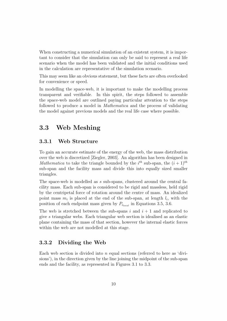
When constructing a numerical simulation of an existent system, it is impor-tant to consider that the simulation can only be said to represent a real lifescenario when the model has been validated and the initial conditions usedin the calculation are representative of the simulation scenario.
This may seem like an obvious statement, but these facts are often overlookedfor convenience or speed.
In modelling the space-web, it is important to make the modelling processtransparent and verifiable. In this spirit, the steps followed to assemblethe space-web model are outlined paying particular attention to the stepsfollowed to produce a model in Mathematica and the process of validatingthe model against previous models and the real life case where possible.
3.3 Web Meshing
3.3.1 Web Structure
To gain an accurate estimate of the energy of the web, the mass distributionover the web is discretized [Ziegler, 2003]. An algorithm has been designed inMathematica to take the triangle bounded by the ith sub-span, the (i+ 1)th
sub-span and the facility mass and divide this into equally sized smallertriangles.
The space-web is modelled as s sub-spans, clustered around the central fa-cility mass. Each sub-span is considered to be rigid and massless, held rigidby the centripetal force of rotation around the centre of mass. An idealizedpoint mass mi is placed at the end of the sub-span, at length li, with theposition of each endpoint mass given by Pilocal
in Equations 3.5, 3.6.
The web is stretched between the sub-spans i and i + 1 and replicated togive s triangular webs. Each triangular web section is idealised as an elasticplane containing the mass of that section, however the internal elastic forceswithin the web are not modelled at this stage.
3.3.2 Dividing the Web
Each web section is divided into n equal sections (referred to here as ‘divi-sions’), in the direction given by the line joining the midpoint of the sub-spanends and the facility, as represented in Figures 3.1 to 3.3.
10

Figure 3.1: 0 divisions Figure 3.2: 1 division Figure 3.3: 2 divisions
For each of the n web sections;
triangles = (n+ 1)2
triangles in top row = 2n+ 1row configuration = {2n+ 1, 2(n− 1) + 1,
2(n− 2) + 1, . . . , 3, 1}number of rows = n+ 1nodes = 1
2(n+ 2)(n+ 3)
midpoints = (n+ 1)2
3.3.3 Web Divisions
A point mass is placed at each mid-point, therefore the total number ofmasses for the webs are s(n+ 1)2, where s is the number of sub-spans. Thatis to say, the number of masses in the web increases as the square of thenumber of divisions. This can lead to a very large number of mass points toconsider for a fine-grain web.
Assembling the space-web with three sub-spans (n = 3) and 0 divisions givesthe layout shown in Figure 3.4, with Figure 3.5 showing the same layout with1 division, and finally Figure 3.6 shows the same layout with 2 divisions. Eachred dot is a mass-point on the web.
Figure 3.4: 3 sub-spans- 0 divs
Figure 3.5: 3 sub-spans- 1 div
Figure 3.6: 3 sub-spans- 2 divs
The space-web layout may be expanded to analyse different web configura-
11

tions. A square layout with 1 division per section is shown in Figure 3.7; apentagonal layout with 2 divisions per section is shown in Figure 3.8; anda hexagonal layout with 3 divisions per section is shown in Figure 3.9 withtotal of 103 masses1.
Figure 3.7: 4 sub-spans- 1 div
Figure 3.8: 5 sub-spans- 2 divs Figure 3.9: 6 sub-spans
- 3 divs
3.4 Equations of Motion
3.4.1 Centre of Mass Modelling
In a real world scenario, the mass of the web is likely to be unevenly dis-tributed. Modelling this requires an expression for the centre of mass (CoM)position, in this case using the facility mass as the origin.
For n masses with positions {Xi, Yi, Zi}, the position of the Centre of Massabout the Facility, in terms of the local {X,Y, Z} coordinate system centredon the Facility mass, is:
PFacility→CoM
n∑
i=1MiXi
n∑
i=1Mi
,
n∑
i=1MiYi
n∑
i=1Mi
,
n∑
i=1MiZi
n∑
i=1Mi
(3.1)
This is used in later equations by taking the position from the Centre ofMass to the Facility mass, as PCoM→Facility = −PFacility→CoM
1103 masses = 96 web midpoints + 6 sub-span masses + 1 central facility mass
12

CoMP_s−1
P_s
Facility
P_1
P_2
P_3
Figure 3.10: Simplified Space-web layout with s sub-spans
3.4.2 Rotations
Rotational matrices are used to rotate the starting vectors to their positionson the local and inertial planes. The local position vector in Equation 3.5is the matrix product of a series of rotations. A diagram of the space-webconfiguration is shown in Figure A.1 with the web removed for clarity.
Rψi,X =
1 0 00 cos[ψi] − sin[ψi]0 sin[ψi] cos[ψi]
(3.2)
Rαi,Y =
cos[αi] 0 sin[αi]0 1 0
− sin[αi] 0 cos[αi]
(3.3)
13
(i,j+1)
(i+1,j)
(i,j)
L2
L2
h
2h3
3
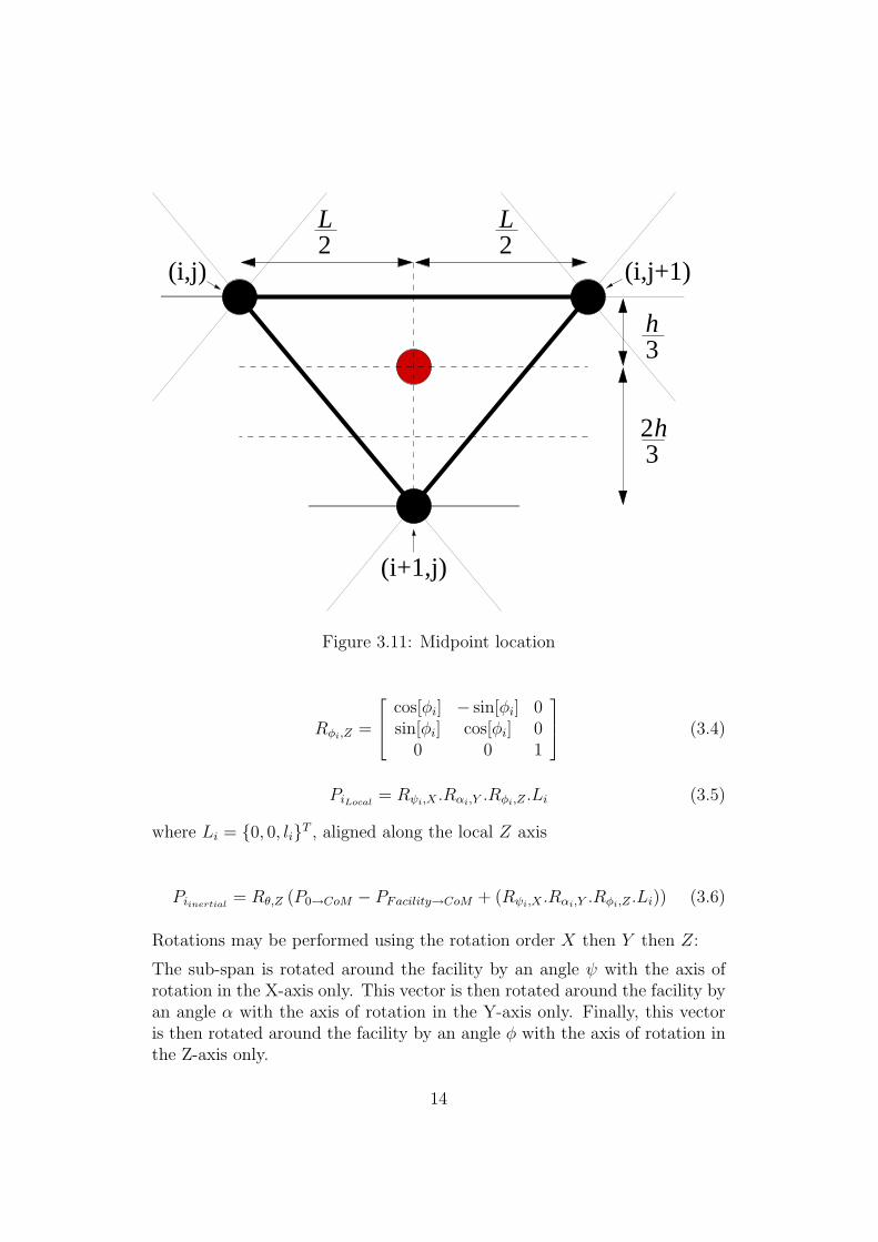
Figure 3.11: Midpoint location
Rφi,Z =
cos[φi] − sin[φi] 0sin[φi] cos[φi] 0
0 0 1
(3.4)
PiLocal= Rψi,X .Rαi,Y .Rφi,Z .Li (3.5)
where Li = {0, 0, li}T , aligned along the local Z axis
Piinertial= Rθ,Z (P0→CoM − PFacility→CoM + (Rψi,X .Rαi,Y .Rφi,Z .Li)) (3.6)
Rotations may be performed using the rotation order X then Y then Z:
The sub-span is rotated around the facility by an angle ψ with the axis ofrotation in the X-axis only. This vector is then rotated around the facility byan angle α with the axis of rotation in the Y-axis only. Finally, this vectoris then rotated around the facility by an angle φ with the axis of rotation inthe Z-axis only.
14

The angles are projected about their respective axes i.e., the Z-rotation, φ,is contained in the X − Y plane. The angles themselves can be comparedto the standard aerospace rotations, with the sub-span direction from thefacility to the edge taken as the tail-nose direction. In this case: ψ is theyaw angle, in the plane of the space-web; α is the pitch angle, out of thespace-web plane; and φ is the roll angle, the twist in the sub-span.
Considering rotations about the ψ direction only - that is constraining themotion of the space-web to be in-plane - gives the following equation
Piinertial= Rθ,Z (P0→CoM − PFacility→CoM + (Rψi,X .Li)) (3.7)
Where P0→CoM = {R, 0, 0}, and represents the position of the Centre of Massfrom Earth and Rψi,X is the rotation of the sub-span about the central facilitygiven by Equation 3.2.
3.4.3 Position equations
The positions of the masses in the local coordinate system must be translatedand rotated into the inertial (Earth centred) coordinate system. The localposition vectors are added to the position vector from the CoM to the Facilityand the position vector from the Earth to the CoM. The resultant vector isthen rotated into the Earth centred Inertial axis system.
3.5 Energy Modelling
For every mass point in the system with position in the inertial frame, Pi,the following steps are undertaken in order to find the Lagrangian energyexpression L:
the respective velocities, Vi are found:
Vi =∂
∂tPi (3.8)
the kinetic energies (linear Tlin and rotational Trot) are obtained and summed:
Tlin =n∑
i=1
1
2miVi.Vi (3.9)
15
Trot =n∑
i=1
mi
1
2Pilocal
.Pilocal
(ψ′
1 + ψ′
2 + ψ′
3)2
3(3.10)
the potential energies, U , are obtained and summed:
U =n∑
i=1
µmi√Pi.Pi
(3.11)
and the Lagrangian is found:
L = Trot + Tlin − U (3.12)
The moment of inertia of each mass point on the web is calculated using theparallel axis theory about the central facility, then multiplied by the squareof the average angular velocities of the three sub-spans to give the rotationalkinetic energy.
The average angular velocity of the three sub-spans, as shown in Equation3.13, was chosen in preference to the actual calculated angular velocities ofeach mass point to simplify the Lagrangian energy expression and to lightenthe computational load. Instead of 27 individual angular velocities, everymass point on the web was assumed to have one common angular velocity.There is an error in this assumption, but this will be acceptably small becausethe actual velocity is approximately equal to the average velocity.
(
∂ψ
∂t
)
ave
=1
3(∂ψ1
∂t+∂ψ2
∂t+∂ψ3
∂t) (3.13)
For each mass point, the Lagrangian energy expression is constructed byconsidering the total kinetic and potential energies of the system.
d
dt(∂T
∂qj) − ∂T
∂qj+∂U
∂qj= Qj (3.14)
Lagrange’s Equations are generated for all the generalised coordinates asspecified in Equation 3.14.
The elastic force the web imparts on the sub-span ends are modelled as asimple elastic tether [Miyazaki and Iwai, 2004], obeying Hooke’s Law;F = Kx:
16

F = K(
H[
(Pi − Pi+1) −2π
s
])
(3.15)
where H[. . . ] is the Heaviside function.
The forces are then used to calculate the right hand side of Lagrange’s Equa-tions, Qi, through consideration of the virtual work.
3.5.1 Simplifying Assumptions
To solve the full set of Lagrange’s Equations for this space-web system in areasonable time on a desktop PC requires some simplifying assumptions tobe made.
Firstly, five generalised coordinates are chosen defining the space web rotatingin the plane normal to the radius vector: (R, θ, ψ1, ψ2, ψ3). The diagram inFigure A.1 shows the layout of the space-web, where R is the orbital Radius,θ is the true anomaly, ψn is the angle between the nth sub-span and the Xlocal
coordinate system.
If the out-of-plane motion of the space-web were to be included, this wouldincrease the number of generalised coordinates to eight, as each sub-spanmust have the out-of-plane motion defined.
If the space-web orbits exclusively in-plane, a simplifying assumption maybe performed in terms of the potential energy expression:
U =n∑
i=1
µmi
R(3.16)
3.5.2 Robot Position Modelling
Robots may move across the space-web in order to reconfigure the web orother tasks as discussed previously. To model this as an kinetic energy basedterm while retaining the flexibility of defining the path without hard-codingthis into the equations, the robot position vector needs to be kept in a verygeneral form.
The robot position vector in Equation 3.17 is defined similarly to Equation3.6: a vector addition of the R vector, the CoM vector and the vector definingthe local position of the robot where
17

{PRobotX , PRobotY , PRobotZ}local are the local vector positions of the robotin the X,Y, Z axes with the origin coincident on the facility mass.
PRobotinertial = Rθ,Z(P0→CoM − PFacility→CoM+{PRobotX , PRobotY , PRobotZ}local) (3.17)
The robot local position vector may be a function of time, position of thesub-span masses (ψ1, ψ2, ψ3), an arbitrary path function or any other smoothgeneralised function.
The kinetic energies of the robot (both linear and rotational) are derived fromthe positions of the robot as before. Both the Lagrangian energy expressionand Lagrange’s Equations contain terms for the local position, velocity, andacceleration of the robots.
Keeping the robot position functions in the most general form allows forrapid reconfiguration of the robot paths and may lead to, for example, robotcontrol studies in the future.
18

Chapter 4
Space-web Dynamics
4.1 Dynamical Simulation
The space-web dynamics are heavily governed by the centre-of-mass move-ment of the system. The space-web system is very rarely symmetrical (bothin reality and in simulations) and this asymmetry can lead to unstable andeven chaotic motion in certain configurations of the space-web.
Several different parameters were considered to be possible influences on thestability of the space-web system, including:
• variation of the masses of the web
• the masses of the robots, the sub-span and facility masses
• the position and velocity of the robots
• the general angular momentum of the robots
• the angular velocity of the web
• and the starting configuration of the web or ‘web symmetry’
4.2 Investigating the Stability of the Space-
web
To test the stability of the space-web with robot movement over the web, twogeneral cases (out of an initial range of six) with different robot movementshave been considered.
19

Firstly, a symmetrical case with three robots moving anticlockwise on theperimeter of the web, is shown in Figure A.20, labelled ‘Case 1’. Secondly,a single robot moving from the central facility to the outer edges of the webalong the first sub-span, is shown in Figure A.21, labelled ‘Case 6’. Bothfigures may be found in the Appendix.
Clearly, the robot movement will have an impact on the stability, but thereare many factors to be considered alongside this. As momentum is a vectorquantity, the sum of the robot’s momentum is more important than a singlerobot. For example, it is possible that three symmetrical robots moving withcoordinated trajectories may perturb the web less than a single moving robot.
4.2.1 Mass of the web
The mass of the web was found to have a negative impact on the stability ofthe system. The higher the mass of the web, the more likely the triangle isto deform from the perfect equilateral shape, and the more likely the systemis to exhibit chaotic motion. This is likely to have been due to the increasein the ratio of the web mass to the other masses, causing the web mass todominate the other mass terms. Figures A.2, A.3, A.4, A.5, A.6 and A.7demonstrate this effect, which were simulated with Case 1∗ in which only themass of the web is varied.
Runs 5-8 show the space-web can be stabilised while the robots move acrossthe surface, the mass of the web increasing to a critical value of approximately25% of the total system mass. The maximum CoM displacement is 0.78mfor these four runs. In runs 9-10, the mass of the web is increased to 40kgand 48kg respectively. This causes significant instability in the web for the48kg web, showing that for certain configurations of the space-web system,the mass of the web is a critical parameter.
4.2.2 Robot crawl velocity
The faster the robots travelled along the web, the greater the likelihoodof unstable behaviour of the web, as the CoM displacement plots show inFigures A.18 and A.19. Both are simulated with Case 6 - asymmetricalrobot paths.
When robot crawl velocity was reduced from 1.0m/s to 0.1m/s, keeping therun time fixed at 1000s, the maximum CoM displacement was reduced by
∗runs 5-11 B, with symmetrical robot paths
20
more than an order of magnitude - from 30m to 1m.
These two cases of mass dependant stability and velocity dependant stabilityare clearly energy related. The higher the energy contained in the system,the more likely the system is to exhibit unstable behaviour. This boundaryhas not yet been clearly defined. Generally speaking, however, the slower therobot movement across the web, the more likely the web is to remain stable.
4.2.3 Robot mass
The momentum of the robot was thought to be a significant parameter inthe stability of the space-web, therefore the robot mass was investigated as apossible parameter. Runs 18-21 tested values of Mrobot from 10kg to 100kg∗
and the CoM positions are shown in Figures A.8, A.9, A.10 and A.11.
Increasing the mass of the robot did not cause any major instabilities inthe space-web system for the narrow range of initial conditions tested. Thisdid have the unintended effect of highlighting a resonance between the robotmovement and the system. For the 10kg and 20kg robots, the system CoMlocation can be seen to orbit with a cam-like locus. The 50kg and 100kgrobots caused the CoM of the system to describe an epitrochoid shape, ratherlike the rotor of a Wankel engine.
4.2.4 Web Asymmetry
The single biggest driver of instability on the space-web system was foundto be the asymmetry in the web configuration and mass distribution.
Very small asymmetries in the initial conditions of the space-web (comparedto a perfectly symmetrical equilateral triangle) are amplified in certain con-figurations of the space-web, and may create large instabilities in the system,especially for energetic configurations such as high web mass and/or largeangular velocities. A small difference in orientation (on the order of 1◦) ofthe sub-spans may lead to large asymmetries between the sub-spans in arelatively short time (≈ 100s).
The cases chosen to investigate the effect of asymmetry on the web are asfollows:
• Case 1: Robots 1,2,3 walk along the edges of the web from sub-span tonext sub-span - (symmetrical)
∗from 3.4% to 17.1% of the system mass
21

• Case 2: Robots 2,3 walk along the edges of the web while Robot 1 isstationary on sub-span 1 - (unsym.)
• Case 3: Robot 3 walks along the edges of the web while Robots 1,2 arestationary on sub-spans 1,2- (unsym.)
• Case 4: Robots 1,2,3 walk along from the centre to their sub-spans -(sym.)
• Case 5: Robot 1 spirals outwards from the centre to the edges, Robots2,3 are fixed on sub-spans (unsym.)
• Case 6: Robot 1 walks along from the centre to sub-span1, Robots 2,3remain in centre (unsym.)
Cases 1 and 4 are symmetrical, shown in Figures A.12 and A.12. These havea stable CoM position throughout the simulation, with a maximum CoMtravel of only 0.6m. In contrast, Cases 2, 3, 5 and 6 are asymmetrical, shownin Figures A.13, A.14, A.16, and A.17. The asymmetric cases show a largeCoM movement of between 15m and 40m, and are unstable.
Compounding the problem of uneven mass, the initial conditions of the threesub-spans were found to influence the stability of the system. The equationscould not be solved with ψ = {0◦, 120◦, 240◦} or spacing the web sub-spans byexactly 120◦, for reasons not known at this time. Initial conditions for ψ wereimplemented as a triplet; the three sub-span values of {0+ψ, 120◦, 240◦ −ψ}offer a solution to this problem.
More generally, it is expected that for most configurations of the triangularspace-web, holding the three sub-spans permanently rigid at exactly 120◦
separation will be impossible as small perturbations to the web in the spaceenvironment will be constantly experienced.
Adding the effect of many asymmetrical robot masses exacerbates the prob-lem of uneven mass distribution. To remedy this, the space-web must beconfigured to occupy as low an energy state as the mission will allow: lowweb mass; light, slow moving robots; low angular velocity of the web. In thisstate, the asymmetry of the web still exists, but it is kept to a manageablelevel.
22

4.3 Numerical Investigation into Stability
A series of solutions to the space-web equations of motion were examinedto examine the effect of five parameters on the space-web stability. Themass of the web, Mweb, the mass of the three daughter satellites, Msat,the robot mass, Mrobot, the sub-span angular coordinate, ψ and the averagesub-span angular velocity ∂ψ
∂twere thought to have an effect on the maximum
movement of the Centre of Mass (CoM) of the space-web system. Therefore,the solutions to 36 different sets of initial conditions were found, with 25 = 32runs complemented by 4 centre point runs. The 36 runs were performedin Mathematica, and the results of the maximum CoM displacement wereentered into a statistical package, Design Expert 7.03. Design Expert thenperforms an analysis of variance (ANOVA) calculation on the factorial dataprovided. ANOVA is a collection of statistical models and their associatedprocedures which compare means by splitting the overall observed varianceinto different parts. A 5 degree of freedom model (or less, if requested) isthen extrapolated from the data and analysed for statistical significance.
The five most strongly correlated model parameters were: Mweb−, Msat+,Mweb ∗ ∂ψ
∂t+, Msat ∗Mrobot ∗ ∂ψ
∂t−, Mrobot− and Mrobot ∗Msat−.
ψ+ and ∂ψ
∂t− were statistically relevant in the model, but to a lesser degree
than the other parameters. As they have a stronger effect when combinedwith other variables, the (un)stabilising influence they have may be overtakenby these other factors.
Parameters are shown with a (+) indicating a stabilising effect or a (−)indicating a destabilising effect, with the full table of values located in theAppendix.
As Mweb− has the strongest influence over the model, it would be mostbeneficial to the stability to reduce the mass of the web.
The reverse is true of the daughter satellite mass, Msat+, increasing thisparameter will tend to stabilise the system.
For combinations of main parameters such as Mweb∗ ∂ψ
∂t+, it would be most
beneficial to increase the product to stabilise the system. In this case, theangular momentum of the web will tend to rigidize the system and enhancethe stability.
23

4.3.1 Masses of the Web and Satellite
The influence the masses of the web and the daughter satellites have on theCoM position are shown in the contour graph, Figure 4.1. The contours areshaded from blue (stable) through green and yellow to red (unstable) andfollow the maximum CoM displacement from the central facility.
Design-Expert® Software
CoM DistDesign Points55.7692
0.00324405
X1 = A: MwebX2 = B: Msat
Actual FactorsC: Mrobot = 5.50D: psi = 0.06E: psidot = 0.55
27.00 87.75 148.50 209.25 270.00
2.00
4.00
6.00
8.00
10.00CoM Dist
A: Mweb
B:
Msa
t
10
15
20
25
3035
40
45
4
Figure 4.1: CoM movement while varying Web and Satellite Mass
For the small sample space of initial conditions, the most stable point wouldbe a high satellite mass (> 8kg) and low web mass (< 50kg). A CoMdisplacement of above 10m is unstable, and would be very difficult for arobot to manoeuvre over the surface.
In general terms, this clearly shows the stabilising effect of the mass of thesatellites and the destabilising effect of the mass of the web.
24

4.3.2 Masses of the Web and Robot
The influence the masses of the web and the robot have on the CoM posi-tion are shown in the contour graph, Figure 4.2. The contours are shadedfrom blue (stable) through green and yellow to red (unstable) and follow themaximum CoM displacement from the central facility.
Design-Expert® Software
CoM Dist55.7692
0.00324405
X1 = A: MwebX2 = C: Mrobot
Actual FactorsB: Msat = 6.00D: psi = 0.05E: psidot = 0.10
27.00 87.75 148.50 209.25 270.00
1.00
3.25
5.50
7.75
10.00CoM Dist
A: Mweb
C:
Mro
bot
10
15 2025 30
3540 45
50
Figure 4.2: CoM movement while varying Web and Robot Mass
The relative strengths of the robot and web masses are shown, with themass of the web exerting a much stronger influence over the behaviour of theweb. The stability boundary is shown in the bottom left hand corner of thegraph. A stability margin of 5m is preferable, here the web mass must bekept below 50kg and the mass of the robot, although less influential, wouldbe best suited at below 5kg. This shows that if a low ∂ψ
∂tis required, the web
can be made more stable with careful consideration of variables.
25
4.3.3 Mass of the Web and Angular Velocity
The influence the masses of the web and the angular velocity, ∂ψ
∂t, have on
the CoM position are shown in the contour graph, Figure 4.3. The contoursare shaded from blue (stable) through green and yellow to red (unstable) andfollow the maximum CoM displacement from the central facility.
Design-Expert® Software
CoM Dist55.7692
0.00324405
X1 = A: MwebX2 = E: psidot
Actual FactorsB: Msat = 10.00C: Mrobot = 1.00D: psi = 0.06
27.00 87.75 148.50 209.25 270.00
0.10
0.33
0.55
0.78
1.00CoM Dist
A: Mweb
E:
psid
ot
5
10
15
20
25
30
35
40
45
50
Figure 4.3: CoM movement while varying Web Mass and ∂ψ
∂t
In a high-stability scenario, the options to configure the space-web are plen-tiful. Carefully choosing the previous parameters that lead to a high proba-bility of stability, namely a high satellite mass (10kg) and a low robot mass(1kg), affords a larger range of possible values for the mass of the web andthe angular velocity of the web.
If the largest acceptable CoM movement is limited to 5m, then there arethree choices available, depending on the primary requirement of the space-web system. If a low web mass is required, then a low ∂ψ
∂tmust match,
and vice versa. Alternatively, if a high mass is required, a high ∂ψ
∂tmust
be specified, and vice versa. The final option is for a low web mass and a
26

high ∂ψ
∂t, affording a large safety margin that may be advantageous in, for
example, a pilot study mission.
4.3.4 Mass of the Robot and Angular Velocity
The influence the mass of the robot and the angular velocity, ∂ψ∂t
, have on theCoM position are shown in the contour graph, Figure 4.4. The contours areshaded from blue (stable) through green and yellow to red (unstable) andfollow the maximum CoM displacement from the central facility.
Design-Expert® Software
CoM Dist55.7692
0.00324405
X1 = C: MrobotX2 = E: psidot
Actual FactorsA: Mweb = 270.00B: Msat = 10.00D: psi = 0.05
1.00 3.25 5.50 7.75 10.00
0.10
0.33
0.55
0.78
1.00CoM Dist
C: Mrobot
E:
psid
ot
5
10
15
20
25
30
35
40
45
50
Figure 4.4: CoM movement while varying Robot Mass and ∂ψ
∂t
The final comparison is for a high mass specification - a 270kg web massand 10kg satellite mass. This combines the two strongest influences on thesystem, the former destabilising and the later stabilising. For a stable system,it is essential to ensure the robot mass is small and the angular rotation rateis large.
27

Chapter 5
Conclusions
5.1 Conclusions
The achievement of a stable, re-configurable web orbiting in space with robotsmoving along its surface is a realistic goal. There must, however, be limitsto the behaviour of the robots and the configuration of the web. Both therobots and the web must be as light as possible and the robots must be as slowmoving as the mission allows, given that this limits the destabilising effectsof these parameters. The daughter satellites must be as heavy as possible,and the angular rotation rate must be as large as possible to maximise thesestabilising effects. In all cases, the web configuration must be as symmetricalas practicable.
5.2 Future Work
To capitalise on the knowledge gained in this research, there are a few areasthat may be expanded on for potential future exploration.
Constructing the web while on orbit would mitigate the deployment phaseof the mission, eliminating one of the major failure modes of the system.Using the robots to weave the web could be inspired by spiders on Earth, forexample, just as the space web has been inspired by the Furoshiki cloth.
Using the knowledge gained through moving masses over the web, there aremany applications that would benefit from simulating web-based construc-tions with moving masses. Solar-sails and antennae could be assembled orreconfigured by robots moving across their surface.
28

Bibliography
I. Bekey. Tethers open new space options, volume 21. NASA, Office of SpaceFlight (1983), 1983.
V.V. Beletsky, E.M. Levin, and American Astronautical Society. Dynamics ofSpace Tether Systems, Advances in the Astronautical Sciences, volume 83.Univelt, August 1993.
M.P. Cartmell. Generating velocity increments by means of a spinning mo-torised tether. 34th AIAA/ASME/SAE/ASEE Joint Propulsion Confer-ence and Exhibit, Dayton, Ohio, USA, 98-3739, 13-15 July 1998.
M.P. Cartmell and S.W. Ziegler. Experimental scale model testing of amotorised momentum exchange propulsion tether. In 37th AIAA/AS-ME/SEA/ASEE Joint Propulsion Conference, Salt Lake City, Utah, USA,AIAA 2001-3914, July 2001.
M.P. Cartmell, C.R. McInnes, and D.J. McKenzie. Proposals for a contin-uous earth-moon cargo exchange mission using the motorised momentumexchange tether concept. Proc. XXXII International Summer School andConference on Advanced Problems in Mechanics, APM2004, pages 72–81,June 24 - July 1 2004.
M. L. Cosmo and E. C. Lorenzini. Tethers in Space Handbook (3rd ed). Num-ber 3. NASA Marshall Space Flight Center, Cambridge, MA, December1997. URL http://www.tethers.com/papers/TethersInSpace.pdf.
Mario L. Cosmo, Enrico C. Lorenzini, and Claudio Bombardelli. Space teth-ers as testbeds for spacecraft formation-flying. Advances in the Astronau-tical Sciences, 119(SUPPL):1083 – 1094, 2005. ISSN 0065-3438.
C.H Draper. Feasibility of the Motorised Momentum Exchange Tether Sys-tem. PhD thesis, University of Glasgow, June 2006.
R.L. Forward and R.P. Hoyt. Failsafe multiline hoytether lifetimes. 1stAIAA/SAE/ASME/ASEE Joint Propulsion Conference, San Diego, CA,AIAA Paper 95-28903, July 1995.
Hironori A. Fujii, Takeo Watanabe, Tairou Kusagaya, Masanori Ohta, andDaisuke Sato. Dynamics of a crawler mass of space tether system. In25th International Symposium on Space Technology and Science (ISTS),
29

Kanazawa, Japan, 2006.P.E. Glaser. Power from the sun, its future. Science, 162(3856):857–861,
1968.N. Kaya, M. Iwashita, S. Nakasuka, L. Summerer, and J. Mankins. Crawling
robots on large web in rocket experiment on furoshiki deployment. 55thInternational Astronautical Congress, Vancouver, Canada, 2004a.
N. Kaya, S. Nakasuka, L. Summerer, and J. Mankins. International rocketexperiment on a huge phased array antenna constructed by furoshiki satel-lite with robots. In 24th International Symposium on Space Technology andScience, Miyazaki, Japan, 2004b.
Shinji Masumoto, Kuniyuki Omagari, Tomio Yamanaka, , and Saburo Matu-naga. System configuration of tethered spinning solar sail for orbital exper-iment - numerical simulation and ground experiment. In 25th InternationalSymposium on Space Technology and Science (ISTS), Kanazawa, Japan,2006.
C.R. McInnes. Solar Sailing: Technology, Dynamics and Mission Applica-tions. Springer Praxis Publishing, 1999.
D.J. McKenzie and M.P. Cartmell. On the performance of a motorized tetherusing a ballistic launch method. 55th International Astronautical Congress,Vancouver, Canada, (IAC-04-IAA-3.8.2.10), Oct. 4-8 2004.
A.K. Misra. Equilibrium configurations of tethered three-body systems andtheir stability. The Journal of the Astronautical Sciences, 50(3):241–253,2002.
Y. Miyazaki and Y. Iwai. Dynamics model of solar sail membrane. In ISAS14th Workshop on Astrodynamics and Flight Mechanics, 2004.
C. Murray, M.P. Cartmell, G. Radice, and M. Vasile. A mechanism for thecontinuous exchange of resources between the earth and the moon usinga hybrid of symmetrically laden motorised momentum exchange tethersand conventional chemical propulsion systems. Technical report, Alenia-Alcatel, Departments of Mechanical & Aerospace Engineering, Universityof Glasgow, 2006.
T. Nakano, O. Mori, and J. Kawaguchi. Stability of spinning solar sail-craftcontaining a huge membrane. AIAA Guidance, Navigation, and ControlConference and Exhibit, pages AIAA–2005–6182, 2005.
G. B. Palmerini, S. Sgubini, and M. Sabatini. Space webs based on rotatingtethered formations. In 57th International Astronautical Congress, Valen-cia, Spain, 2-6th October 2006.
Gunnar Tibert and Mattias Gardsback. Space-webs. Technical report, KTHand ESA ACT, 2006.
S.W. Ziegler. The Rigid Body Dynamics of Tethers in Space. PhD thesis,Department of Mechanical Engineering, University of Glasgow, 2003.
30

S.W. Ziegler and M.P. Cartmell. Using motorized tethers for payload orbitaltransfer. Journal of Spacecraft and Rockets, 38(6):904–913, 2001.
31

Appendix A
Graphics
θ
ψ1ψ2
ψ3
localX
Xinertial
Yinertial
localY
Earth
��������
Facility
Radius of CoM
Orbital Path of
Space−Web CoM
Mass1
Mass3
Mass2
����
��CoM
Figure A.1: Space-web diagram with 3 sub-spans shown in Inertial Space
32

A.1 Case 1 - CoM plots of stability while in-
creasing web mass
-0.3 -0.2 -0.1 0 0.1 0.2 0.3
-0.3
-0.2
-0.1
0
0.1
0.2
0.3
Y
ZCoM Position
Figure A.2: mWeb = 27kg
-0.4 -0.2 0 0.2 0.4
-0.4
-0.2
0
0.2
0.4
Y
ZCoM Position
Figure A.3: mWeb = 34kg
-0.75 -0.5 -0.25 0 0.25 0.5 0.75
-0.75
-0.5
-0.25
0
0.25
0.5
0.75
Y
ZCoM Position
Figure A.4: mWeb = 38kg
-0.4 -0.2 0 0.2 0.4-0.4
-0.2
0
0.2
0.4
Y
ZCoM Position
Figure A.5: mWeb = 40kg
-3 -2 -1 0 1 2 3-3
-2
-1
0
1
2
3
Y
ZCoM Position
Figure A.6: mWeb = 45kg
-15 -10 -5 0 5 10 15 20
-10
-5
0
5
10
15
Y
ZCoM Position
Figure A.7: mWeb = 48kg
33

A.2 Case 1 - CoM plots of stability while in-
creasing robot mass
-0.6 -0.4 -0.2 0 0.2 0.4-0.6
-0.4
-0.2
0
0.2
0.4
0.6
Y
ZCoM Position
Figure A.8: Mrobot = 10kg
-0.4 -0.2 0 0.2 0.4 0.6-0.6
-0.4
-0.2
0
0.2
0.4
0.6
Y
ZCoM Position
Figure A.9: Mrobot20kg
-0.6 -0.4 -0.2 0 0.2 0.4 0.6
-0.6
-0.4
-0.2
0
0.2
0.4
0.6
Y
ZCoM Position
Figure A.10: Mrobot50kg
-0.6 -0.4 -0.2 0 0.2 0.4 0.6
-0.6
-0.4
-0.2
0
0.2
0.4
0.6
Y
ZCoM Position
Figure A.11: Mrobot10kg
34

A.3 CoM plots of stability while changing
robot paths
-0.6 -0.4 -0.2 0 0.2 0.4-0.6
-0.4
-0.2
0
0.2
0.4
0.6
Y
ZCoM Position
Figure A.12: Case F1
-15 -10 -5 0 5 10 15-15
-10
-5
0
5
10
15
Y
ZCoM Position
Figure A.13: Case F2
-15 -10 -5 0 5 10 15
-15
-10
-5
0
5
10
15
Y
ZCoM Position
Figure A.14: Case F3
-0.4 -0.2 0 0.2 0.4
-0.4
-0.2
0
0.2
0.4
Y
ZCoM Position
Figure A.15: Case F4
-40 -20 0 20 40
-40
-20
0
20
40
Y
ZCoM Position
Figure A.16: Case F5
-20 -10 0 10 20
-20
-10
0
10
20
Y
ZCoM Position
Figure A.17: Case F6
35

A.4 Case 6 - CoM plots of stability while de-
creasing robot velocity
-20 -10 0 10 20
-20
-10
0
10
20
Y
ZCoM Position
Figure A.18: Vrobot = 1.0m/s
-1 -0.5 0 0.5 1
-1
-0.5
0
0.5
1
Y
ZCoM Position
Figure A.19: Vrobot = 0.1m/s
36
-100
-50
050
100
X
-100
-50
0
50
100Y
-100
-50
0
50
100
Z
-100
-50
0
50
Figure A.20: Case 1 – 3 Robots moving symmetrically round the web perime-ter
37

-100
-50
050
100
X
-100
-50
0
50
100Y
-100
-50
0
50
100
Z
-100
-50
0
50
Figure A.21: Case 6 – 1 Robot moving asymmetrically along first sub-span
38

Appendix B
Data
Data generated during the first run phase - initially examining the dynamicsof the space-web.
The units for the variables are as follows:
Mweb Msat MRobot psi dpsi/dt k CoM dispkg kg kg degrees radians N/m m
The ICs of selected other parameters are:
L = 100.0m ; Mfacility = 100.0kg ; eccent = 0.0 ; tend = 100.0s ; R =6.578 ∗ 106m
39

run Case Mweb Msat MRobot psi dpsi/dt k CoM disp Pred CoM Diff%1 1 27 10 10 0.1 0.1 1227 0.04 -0.47 -1179%2 1 27 10 1 0.1 0.1 1227 0.03 -0.59 -18493 1 270 2 2 0.1 0.1 1227 45.00 48.34 1074 1 270 10 2 0.01 1.0 1227 50.00 -287.35 -5755 1 27 1 2 1 0.1 122.7 0.35 42.21 120596 1 33.75 1.25 2 1 0.1 122.7 0.42 40.20 95727 1 37.8 1.4 2 1 0.1 122.7 0.78 39.04 50058 1 40.5 1.5 2 1 0.1 122.7 0.39 38.29 99459 1 44.82 1.66 2 1 0.1 122.7 3.80 37.11 977
10 1 47.5 1.759259 2 1 0.1 122.7 20.00 36.40 18211 1 54 2 2 1 0.1 122.7 34.00 34.73 10212 1 27 1 2 1 0.1 122.7 0.51 42.21 827613 1 54 2 2 1 0.1 122.7 0.52 34.73 667914 1 135 5 2 1 0.1 122.7 0.55 21.07 383015 1 270 10 10 1 0.1 122.7 0.60 50.70 845016 1 540 20 10 1 0.1 122.7 0.63 851.23 13619717 1 135 5 10 1 0.1 122.7 0.59 -28.33 -480218 1 135 10 10 1 0.1 122.7 0.59 -135.91 -2303519 1 135 10 20 1 0.1 122.7 0.62 -298.99 -4822420 1 135 10 50 1 0.1 122.7 0.68 -788.24 -11591721 1 135 10 100 1 0.1 122.7 0.75 -1603.65 -21381922 1 27 10 10 1 0.1 122.7 0.41 -285.19 -6956023 2 27 10 10 0.1 0.1 1227 6.00 -0.47 -824 2 27 10 1 0.1 0.1 1227 3.00 -0.59 -2025 2 135 10 10 1 0.1 122.7 15.00 -135.91 -90626 3 27 10 10 0.1 0.1 1227 6.00 -0.47 -827 3 27 10 1 0.1 0.1 1227 3.10 -0.59 -1928 3 135 10 10 1 0.1 122.7 17.50 -135.91 -77729 4 27 10 10 0.1 0.1 1227 0.03 -0.47 -157230 4 27 10 1 0.1 0.1 1227 0.03 -0.59 -215131 4 135 10 10 1 0.1 122.7 0.48 -135.91 -2861232 5 27 10 10 0.1 0.1 1227 30.00 -0.47 -233 5 27 10 1 0.1 0.1 1227 3.50 -0.59 -1734 5 135 10 10 1 0.1 122.7 52.00 -135.91 -26135 6 135 10 10 1 0.1 122.7 26.00 -135.91 -52336 6 135 10 10 1 0.5 122.7 28.00 -913.47 -326237 6 2.7 10 5 1 0.5 122.7 1.10 -862.14 -78377
40

Data generated during the numerical investigation into stability.
run A:Mweb B:Msat C:Mrobot D:psi E:psidot F: CoM posn predicted Diff %1 27 2 1 0.01 0.1 11.49 12.29 107%2 270 2 1 0.01 0.1 49.41 46.71 95%3 27 10 1 0.01 0.1 0.00 -2.70 -83118%4 270 10 1 0.01 0.1 52.76 53.56 102%5 27 2 10 0.01 0.1 28.09 25.39 90%6 270 2 10 0.01 0.1 53.20 54.00 102%7 27 10 10 0.01 0.1 0.00 0.80 19141%8 270 10 10 0.01 0.1 55.75 53.05 95%9 27 2 1 0.1 0.1 11.28 10.16 90%
10 270 2 1 0.1 0.1 49.83 47.37 95%11 27 10 1 0.1 0.1 0.03 0.12 369%12 270 10 1 0.1 0.1 52.79 51.67 98%13 27 2 10 0.1 0.1 27.49 26.72 97%14 270 2 10 0.1 0.1 52.99 51.65 97%15 27 10 10 0.1 0.1 0.04 -0.05 -111%16 270 10 10 0.1 0.1 55.61 54.83 99%17 148.5 6 5.5 0.055 0.55 47.15 31.10 66%18 148.5 6 5.5 0.055 0.55 47.15 31.10 66%19 148.5 6 5.5 0.055 0.55 47.15 31.10 66%20 148.5 6 5.5 0.055 0.55 47.15 31.10 66%21 27 2 1 0.01 1 49.41 46.71 95%22 270 2 1 0.01 1 49.86 50.66 102%23 27 10 1 0.01 1 0.00 0.80 24649%24 270 10 1 0.01 1 0.00 -2.70 -64127%25 27 2 10 0.01 1 33.10 33.90 102%26 270 2 10 0.01 1 49.41 46.71 95%27 27 10 10 0.01 1 49.83 47.13 95%28 270 10 10 0.01 1 55.77 56.57 101%29 27 2 1 0.1 1 49.41 48.63 98%30 270 2 1 0.1 1 49.82 48.69 98%31 27 10 1 0.1 1 0.03 -1.09 -3346%32 270 10 1 0.1 1 0.03 -0.74 -2287%33 27 2 10 0.1 1 33.11 31.98 97%34 270 2 10 0.1 1 49.41 48.63 98%35 27 10 10 0.1 1 0.00 -0.77 -18329%36 270 10 10 0.1 1 55.76 54.63 98%
The ICs of selected other parameters are:
L = 100.0m ; Mfacility = 100.0kg ; eccent = 0.0 ; tend = 100.0s ; R =6.578 ∗ 106m
Note: the percentage change (= predicted CoM / simulated CoM) may bevery large due to the small simulated CoM displacement.
41

Data generated during the numerical investigation into stability.
Term Effect Stdized Effect SumSqr % Contribtn
A-Mweb - 27.21 7182.9 37.72
B-Msat + -16.57 2447.8 12.85
AE + -15.32 1869.6 9.82
BCE - 14.34 1656.8 8.70
C-Mrobot - 10.90 872.3 4.58
BC - 9.93 666.4 3.50
BE + -8.69 686.3 3.60
AB - 7.21 435.0 2.28
ACE - 6.98 346.3 1.82
CE - 5.04 232.9 1.22
AC - 4.66 193.2 1.01
ABE + -3.76 118.3 0.62
ABC - 3.75 118.6 0.62
BDE + -3.37 93.4 0.49
ADE - 3.29 117.6 0.62
ABCDE - 3.19 85.1 0.45
ACD - 3.17 99.5 0.52
BCD + -3.15 102.7 0.54
CDE + -3.12 92.4 0.49
ABDE - 3.12 81.5 0.43
CD + -3.09 110.1 0.58
D-psi + -3.08 79.6 0.42
BCDE + -3.08 83.7 0.44
ACDE - 3.04 89.0 0.47
ABCD - 3.02 61.5 0.32
DE + -3.00 75.6 0.40
ABD - 2.97 74.0 0.39
AD - 2.93 98.7 0.52
BD + -2.84 34.2 0.18
E-psidot - 1.48 18.3 0.10
Lack Of Fit 9.6 0.05
Pure Error 0.0 0.00
The ‘Effect’ term in column 2 is a reflection on the stabilising (+) or desta-bilising (−) effect of the term.
42