ARTICLE IN PRESS

Contents lists available at ScienceDirect

Signal Processing

Signal Processing 89 (2009) 2103–2116

0165-16

doi:10.1

$ Thi

at EUSI

MIMO

Tensor

Ma 544� Cor

E-m

favier@

journal homepage: www.elsevier.com/locate/sigpro

Space–time spreading–multiplexing for MIMO wirelesscommunication systems using the PARATUCK-2 tensor model$

Andre L.F. de Almeida a,b, Gerard Favier a,�, Joao C.M. Mota b

a I3S Laboratory, University of Nice-Sophia Antipolis, CNRS, Franceb GTEL-Wireless Telecom Research Group, Federal University of Ceara, Fortaleza, Brazil

a r t i c l e i n f o

Article history:

Received 28 October 2008

Received in revised form

16 February 2009

Accepted 16 April 2009Available online 3 May 2009

Keywords:

MIMO systems

Space–time spreading

Multiplexing

Blind detection

Tensor modeling

PARATUCK-2 model

84/$ - see front matter & 2009 Elsevier B.V. A

016/j.sigpro.2009.04.028

s paper is an extended version of our conferen

PCO’08 and entitled ‘‘Space–Time Spreadin

Antenna Systems with Blind Detection usin

Model’’. This work was supported by CAPES-C

/07.

responding author. Tel.: +33 492 942 736; fax:

ail addresses: andre@gtel.ufc.br (A.L.F. de Alm

i3s.unice.fr (G. Favier), mota@gtel.ufc.br (J.C.M

a b s t r a c t

In this paper, we present a new space–time spreading–multiplexing model for multiple-

input multiple-output (MIMO) wireless communication systems relying on a tensor

modeling of the transmitted and received signals. At the transmitter, we exploit the core

of a PARATUCK-2 tensor model composed of a precoding matrix and two allocation

matrices that allow to control the spreading and multiplexing of the data streams across

the space dimension (transmit antennas) and time-dimension (time-slots). Different

MIMO schemes combining space–time multiplexing and diversity can be derived from

the proposed model. The identifiability and uniqueness of the PARATUCK-2 tensor

model for the received signal are discussed and subsequently exploited for a joint blind

channel estimation and symbol detection. The bit-error-rate performance of different

transmit schemes derived from the proposed tensor model is evaluated by means of

computer simulations.

& 2009 Elsevier B.V. All rights reserved.

1. Introduction

It is well known for some time that multiple-inputmultiple-output (MIMO) wireless communication sys-tems employing multiple antennas at both the transmitterand the receiver provide multiplexing gains [1] and/ordiversity gains [2] to increase the data rate (i.e. higherspectral efficiency) and/or the reliability of the transmis-sion (i.e. lower error rate) without additional bandwidth.In order to provide multiple-accessing capabilities toMIMO systems, several approaches make use of code-division multiple-access (CDMA) technology by associat-ing multiple transmit antennas and multiple user signals

ll rights reserved.

ce paper presented

g–Multiplexing for

g the PARATUCK-2

OFECUB, project no

+33 492 942 896.

eida),

. Mota).

to orthogonal spreading transforms in different manners[3,4]. Optionally, when current channel state is known inadvance at the transmitter, some form of precoding canalso be used to improve system performance [5].

The use of tensor decompositions for modeling MIMOtransceivers with blind signal processing has beenaddressed in several recent works [6,8–12]. The approachof Sidiropoulos and Budampati [6], therein called Khatri–

Rao space–time (KRST) codes, relies on a PARAllel FACtor(PARAFAC) model [7]. By precoding each data stream overmultiple symbol periods, a joint blind channel estimationand symbol detection is afforded by means of a PARAFACmodeling of the received signal tensor. The work [8]presents a generalized block-tensor model for multiple-access MIMO transceivers. The common feature of thesolutions [6] and [8] is the use of pure spatial multi-plexing, where each data stream is transmitted by a singletransmit antenna and coded across the time-dimensiononly. Consequently, no transmit spatial diversity isallowed and the number of data streams is restricted tobe equal to the number of transmit antennas. To overcome

ARTICLE IN PRESS

A.L.F. de Almeida et al. / Signal Processing 89 (2009) 2103–21162104

this limitation, the work in [9] uses a constrained tensormodel which can be viewed as a ‘‘structured’’ PARAFACmodel with an a priori known model structure. This allowsto model, in addition to spatial multiplexing, a wider classof MIMO transmissions characterized by a joint space andtime spreading. In order to cope with multiuser downlinktransmissions, de Almeida et al. [10] formulated a block-constrained version of the tensor model of [9], whichallows a multiuser space–time transmission with differentspatial spreading factors (diversity gains) as well asdifferent multiplexing factors (code rates) for the users.

More general space–time spreading structures wererecently proposed relying on a third-order CONstrainedFACtor (CONFAC) tensor model [11,12]. The approach of deAlmeida et al. [11] introduces two constraint matriceswith variable 1’s and 0’s structure into the tensor model.These constraint matrices are referred therein as streamand code allocation matrices. As opposed to the approachof [9,10] where the two constraint matrices have a fixedstructure, in [11] the structure of the constraint matricescan be controlled to design transmit schemes withdifferent spatial multiplexing, code multiplexing andtransmit antenna assignments for the data streams. Thework [12] further generalizes [11] by including a thirdallocation matrix that defines the mapping of theprecoded signals to the transmit antennas. In this case,the constrained structure of the CONFAC model is fullyexploited at the transmitter (for designing finite-sets ofMIMO transmission schemes) as well as at the receiver(for blind signal processing).

In this work, we present a novel tensor-based space–time spreading–multiplexing model. At the transmitter,we exploit the structure of a PARATUCK-2 tensor model todesign different precoder structures combining space–time multiplexing and diversity. The heart of the proposedtensor model is composed of two constraint matrices.These constraint matrices play the role of stream-to-slotand antenna-to-slot allocation matrices. Differently to theCONFAC model of de Almeida et al. [11,12], the twoallocation matrices of the PARATUCK-2 core tensor jointlycontrol the spatial and temporal allocations, i.e. theallocations of data streams to transmit antennas andtime-slots. Moreover, the number of channel uses asso-ciated with the transmission of each data stream may bedifferent from one data stream to another. Such a featureis not possible with the existing tensor-based space–timetransmission models and is intrinsic to the PARATUCK-2modeling. At the receiver, we capitalize on the structure ofthe PARATUCK-2 model for the received signal to performa joint blind detection and channel estimation. Theidentifiability issue of the proposed tensor model isdiscussed and a simple blind receiver based on thealternating least squares (ALS) algorithm is presented.

The PARATUCK-2 model can be viewed as a general-ization of the PARAFAC one. It mixes the properties of bothPARAFAC [7] and TUCKER-2 [13] models. Consequently, itallows the flexibility of TUCKER-2 model while retainingPARAFAC’s uniqueness properties. This model has beenstudied in the psychometrics literature [14] and subse-quently exploited by Bro [15] to solve special data analysisproblems in chemometrics. The first application of

PARATUCK-2 in signal processing was proposed byKibangou and Favier [16] for the blind joint identificationand equalization of Wiener–Hammerstein communica-tion channels. The present paper shows that this model isalso useful to model the transmitted and received signalsin MIMO wireless communication systems while afford-ing a blind signal processing.

Despite the differences among PARAFAC, CONFAC andPARATUCK-2 modeling approaches, it is worth mentioningthat they share common characteristics. First, they simul-taneously exploit three diversity dimensions (space, time

and code) that characterize the received signal tensor. Eachdiversity dimension is associated with a different matrixfactor of the received signal tensor model as follows:

�

The space dimension is created by the multiple-antennachannel and is associated with the channel matrix. � The time dimension arises by collecting the received

signal during several symbol periods and is associatedwith the symbol matrix.

� The code dimension is generated by precoding each

transmitted symbol across multiple time-slots, and isassociated with the precoder matrix.

The relationship involving channel, symbol and precodermatrices depends on the structure adopted to model thereceived signal tensor. In this work, such a relationship isdefined by the PARATUCK-2 structure. The use of thistensor modeling allows to perform a blind joint symboland channel estimation under identifiability conditionsmore relaxed than those of conventional matrix modelingbased approaches, and without requiring statisticalindependence between transmitted signals. Instead, thereceiver signal processing is deterministic and directlyexploits the known structure of the received signal tensor.Moreover, tensor-based receivers are generally based on ajoint detection of the transmitted signals (either fromdifferent users or from multiple transmit antennas).

We emphasize that the contribution of this work concernsboth transmitter and receiver processing. At the transmitter,the PARATUCK-2 model structure is used to model space–time multiplexing–spreading. At the receiver, this structure isexploited to blindly estimate the transmitted symbols and theMIMO channel. Fig. 1 provides an illustration of the use oftensor models in a MIMO communication chain. The threesignal dimensions that generally appear at the transmitterand receiver are highlighted.

The organization of the rest of this paper is as follows.Section 2 presents a brief overview of the main third-order tensor models. In Section 3, the proposed space–time multiplexing–spreading system is presented and theassociated tensor signal model is formulated. In Section 4,some examples of space–time multiplexing–spreadingdesigns are presented by focusing on the structure ofthe PARATUCK-2 constraint matrices. Section 5 discussesthe identifiability and uniqueness issues of the proposedPARATUCK-2 tensor model. In Section 6, we present ablind PARATUCK-2 based receiver for joint channelestimation and symbol detection. Some simulation results

ARTICLE IN PRESS

TX signal tensor

Input data streams

Transmitter processing(precoding)

RX signal tensor

MIMOchannel

Receiver processing

(signal separation)

Joint blind symbol and

channel estimation

Tensor models(PARAFAC, CONFAC,

PARATUCK-2,...)

SpaceDimension

(Tx)

Time dimension

Code dimenson

Space Dimension

(Rx)

Time dimension

Code dimenson

Fig. 1. Use of tensor models in a MIMO communication chain.

A.L.F. de Almeida et al. / Signal Processing 89 (2009) 2103–2116 2105

are presented in Section 7 to illustrate the performance ofthis blind receiver. This paper is concluded in Section 8.

Notations: Some notations and properties are nowdefined. AT , A�1 and Ay stand for transpose, inverse andpseudo-inverse of A, respectively. The operator diagðaÞforms a diagonal matrix from its vector argument, whileDiðAÞ forms a diagonal matrix holding the i-th row of A onits main diagonal. The Kronecker and the Khatri–Raoproducts are denoted by � and �, respectively,

A � B ¼ ½A�1 � B�1; . . . ;A�R � B�R� ¼

BD1ðAÞ

..

.

BDIðAÞ

26643775 (1)

with A ¼ ½A�1; . . . ;A�R� 2 CI�R, B ¼ ½B�1; . . . ;B�R� 2 C

J�R. Weshall make use of the following property of the Kroneckerproduct:

vecðACBTÞ ¼ ðB� AÞvecðCÞ. (2)

for A 2 CI�R, B 2 CJ�S, and C 2 CR�S. Scalars are denoted bylower case letters ða;b; . . . ;a;b; . . .Þ, vectors are written asboldface lower case letters ða;b; . . .Þ, matrices as boldfacecapitals ðA;B; . . .Þ, and tensors as calligraphic lettersðA;B; . . .Þ.

2. Main third-order tensor models

This section gives a brief overview of the main third-order tensor models: the PARAFAC, TUCKER-3, PARATUCK-2and CONFAC tensor models. The constrained PARATUCK-2model used in this work is more particularly detailed.

2.1. PARAFAC

The PARAllel FACtor model of X 2 CI1�I2�I3 has thefollowing scalar form:

xi1 ;i2 ;i3 ¼XF

f¼1

ai1 ;f bi2 ;f ci3 ;f , (3)

where ai1 ;f ¼ ½A�i1 ;f , bi2 ;f ¼ ½B�i2 ;f and ci3 ;f ¼ ½C�i3 ;f are scalarcomponents of the three matrix factors A 2 CI1�F , B 2CI2�F and C 2 CI3�F , respectively, and F defines the rank ofthe tensor.

2.2. TUCKER-3

The TUCKER-3 model was proposed by Tucker in the1960s [13]. It incorporates most of the other third-ordertensor models as special cases, and it can be written inscalar form as

xi1 ;i2 ;i3 ¼XR1

r1¼1

XR2

r2¼1

XR3

r3¼1

ai1 ;r1bi2 ;r2

ci3 ;r3gr1 ;r2 ;r3

, (4)

where ai1 ;r1¼ ½A�i1 ;r1

, bi2 ;r2¼ ½B�i2 ;r2

and ci3 ;r3¼ ½C�i3 ;r3

arescalar components of the three matrix factors A 2 CI1�R1 ,B 2 CI2�R2 and C 2 CI3�R3 , respectively, and gr1 ;r2 ;r3

¼

½G�r1 ;r2 ;r3is a scalar component of the TUCKER-3 core

tensor G 2 CR1�R2�R3.It is worth noting that TUCKER-3 reduces to PARAFAC

in the case R1 ¼ R2 ¼ R3 ¼ F with gf ;f ;f ¼ df ;f ;f , where df ;f ;f

is the Kronecker delta. In other words, PARAFAC is aspecial case of TUCKER-3 with a diagonal core tensor, themain diagonal being composed of ones.

Special cases: TUCKER-2 and TUCKER-1: The TUCKER-2model arises from the TUCKER-3 one by setting onematrix factor, say C, to the identity matrix. This model istherefore defined as

xi1 ;i2 ;i3 ¼XR1

r1¼1

XR2

r2¼1

ai1 ;r1bi2 ;r2

gr1 ;r2 ;i3, (5)

where gr1 ;r2 ;i3is the scalar component of the TUCKER-2

core tensor G 2 CR1�R2�I3. Similarly, the TUCKER-1 modelarises from the TUCKER-3 one by setting two matrixfactors, say B and C, to identity matrices. In this case,

ARTICLE IN PRESS

A.L.F. de Almeida et al. / Signal Processing 89 (2009) 2103–21162106

we obtain

xi1 ;i2 ;i3 ¼XR1

r1¼1

ai1 ;r1gr1 ;i2 ;i3

, (6)

where gr1 ;i2 ;i3is the scalar component of the TUCKER-1

core tensor G 2 CR1�I2�I3.

2.3. PARATUCK-2

The PARATUCK-2 model of X is defined in scalar formby the following expression:

xi1 ;i2 ;i3 ¼XR1

r1¼1

XR2

r2¼1

ai1 ;r1bi2 ;r2

gr1 ;r2cA

i3 ;r1cB

i3 ;r2, (7)

where xi1 ;i2 ;i3 is the ði1; i2; i3Þ-th entry of tensor X,

ai1 ;r1¼ ½A�i1 ;r1

, bi2 ;r2¼ ½B�i2 ;r2

, cAi3 ;r1¼ ½CA

�i3 ;r1, cB

i3 ;r2¼ ½CB

�i3 ;r2,

and gr1 ;r2¼ ½G�r1 ;r2

are the entries of matrices A 2 CI1�R1 ,

B 2 CI2�R2 , CA2 CI3�R1 , CB

2 CI3�R2 and G 2 CR1�R2 , respec-tively. The matrices A and B are the two matrix factors ofthe model. They are associated with the first and second

dimensions of the tensor X 2 CI1�I2�I3. The matrices CA

and CB are called interaction matrices. They define thelinear combination profile between the R1 columnsof A and the R2 columns of B along the third dimensionof the tensor X. The matrix G is the core matrix of thePARATUCK-2 model. The element gr1 ;r2

of G defines the

magnitude of the interaction between the r1-th columnof A and the r2-th column of B.

Eq. (7) can be rewritten as

xi1 ;i2 ;i3 ¼XR2

r2¼1

XR1

r1¼1

ai1 ;r1cA

i3 ;r1gr1 ;r2

!cB

i3 ;r2bi2 ;r2

¼XR2

r2¼1

Ai1�Di3 ðCAÞG�r2

cBi3 ;r2

bi2 ;r2

¼ Ai1�Di3 ðCAÞGDi3 ðC

BÞBT�i2

. (8)

Let us define the matrix-slices X��i3 2 CI1�I2 , i3 ¼ 1; . . . ; I3,

obtained by ‘‘slicing’’ the tensor along its third dimension:

½X��i3 �i1 ;i2 ¼ xi1 ;i2 ;i3 .

Varying the indices i1 and i2 with i3 fixed in (8) gives thefollowing expression of the matrix-slice X��i3 :

X��i3 ¼ ADi3 ðCAÞGDi3 ðC

BÞBT ; i3 ¼ 1; . . . ; I3, (9)

where Di3 ðCAÞ 2 CR1�R1 and Di3 ðC

BÞ 2 CR2�R2 .

Constrained PARATUCK-2: In this paper, we consider a

special PARATUCK-2 model, where CA and CB are con-strained to have only 1’s and 0’s entries. For instance,

cAi3 ;r1¼ cB

i3 ;r2¼ 1 means that the r1-th column of A interacts

with the r2-th column of B in the generation of the i3-thmatrix-slice X��i3 , the magnitude of this interaction being

determined by the entry gr1 ;r2of the core matrix G.

Otherwise if cAi3 ;r1¼ cB

i3 ;r2¼ 0, it means that there is

no interaction between the corresponding columns ofA and B.

2.4. CONFAC

The constrained factor model of X with F factorcombinations is defined in scalar form as

xi1 ;i2 ;i3 ¼XR1

r1¼1

XR2

r2¼1

XR3

r3¼1

ai1 ;r1bi2 ;r2

ci3 ;r3gr1 ;r2 ;r3

ðW;U;XÞ, (10)

where

gr1 ;r2 ;r3ðW;U;XÞ ¼

XF

f¼1

cr1 ;ffr2 ;f

or3 ;f (11)

is an element of the constrained core tensor GðW;U;XÞ 2CR1�R2�R3 , and W 2 CR1�F , U 2 CR2�F and X 2 CR3�F arethree full row-rank constraint matrices, the columns ofwhich are canonical vectors belonging to canonical basesof dimensions R1, R2 and R3, respectively, withF maxðR1;R2;R3Þ.

By suppressing the constraints, i.e. W ¼ U ¼ X ¼ IF ,and choosing R1 ¼ R2 ¼ R3 ¼ F, the CONFAC model (10)reduces to the PARAFAC one (3). On the other hand,comparing (10) with (4), we observe that CONFAC can beseen as a constrained TUCKER-3 model with the particularcharacteristic of having a PARAFAC-decomposed coretensor as shown in (11). In the TUCKER-3 model, thetensor X is composed of R1R2R3 factor combinations.Differently, in the CONFAC model only F combinationstake place for composing the tensor X. In this case, theF-factor PARAFAC model of the constrained core tensor G,parameterized by W, U and X, defines the pattern ofcombinations, or interactions, involving the columns ofthe matrix factors A;B and C.

Constrained tensor models, which can be viewed ashybrid models between PARAFAC and TUCKER-3, arestudied for some time in the area of chemometrics[15,17–21]. The constraints are generally imposed on theTUCKER-3 core tensor, which may have a large majority ofzero elements [20]. With respect to uniqueness, con-strained tensor models may be ‘‘partially’’ unique (ornonunique in a restrictive sense). Partial uniquenesscan be studied from the pattern of zeros of the coretensor as pointed out by ten Berge and Smilde [19] and tenBerge [20].

Table 1 summarizes the different tensor models inscalar form. The presence of interactions between matrixfactors is also indicated. We remark that these interac-tions are, in general, unconstrained in the TUCKER-3model (a total of R1R2R3 interactions is possible). ForCONFAC, these interactions are controlled by the threeconstraint matrices W, U, and X, whereas for PARATUCK-2the interaction pattern is defined by CA and CB.

In the next section, we exploit the constrainedPARATUCK-2 model to design the structure of the multiple-antenna transmission scheme used at the transmitter.

3. Proposed space–time spreading–multiplexing model

Let us consider a MIMO wireless communicationsystem with M transmit antennas and K receive antennas.At the transmitter, the serial input stream is divided into R

ARTICLE IN PRESS

M

···

···

···

··· ···

···

······

1

Stream-to-slot allocation

Antenna-to-slotallocation

1

Input data streams

Precoded

R

1μ 1γ

Pμ

P/S

P/S

P

P

Pγ

{ }1,1,1 Nss

{ }RNR ss ,,1 (Ψ)

Time-slot 1

Time-slot P

Precoding

Precoding(W)

(W)

(Φ)

symbolsTemporally-allocated

symbols transmitted signalSpace-time

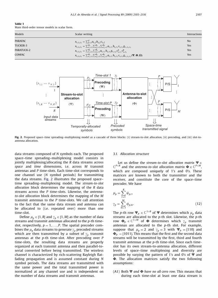
Fig. 2. Proposed space–time spreading–multiplexing model as a cascade of three blocks: (i) stream-to-slot allocation, (ii) precoding, and (iii) slot-to-

antenna allocation.

Table 1Main third-order tensor models in scalar form.

Models Scalar writing Interactions

PARAFAC xi1 ;i2 ;i3 ¼PF

f¼1ai1 ;f bi2 ;f ci3 ;fNo

TUCKER-3 xi1 ;i2 ;i3 ¼PR1

r1¼1

PR2

r2¼1

PR3

r3¼1ai1 ;r1bi2 ;r2

ci3 ;r3gr1 ;r2 ;r3

Yes

PARATUCK-2 xi1 ;i2 ;i3 ¼PR1

r1¼1

PR2

r2¼1ai1 ;r1bi2 ;r2

gr1 ;r2cA

i3 ;r1cB

i3 ;r2

Yes

CONFAC xi1 ;i2 ;i3 ¼PR1

r1¼1

PR2

r2¼1

PR3

r3¼1ai1 ;r1bi2 ;r2

ci3 ;r3gr1 ;r2 ;r3

ðW;U;XÞ Yes

A.L.F. de Almeida et al. / Signal Processing 89 (2009) 2103–2116 2107

data streams composed of N symbols each. The proposedspace–time spreading–multiplexing model consists injointly multiplexing/allocating the R data streams acrossspace and time dimensions, i.e. across M transmitantennas and P time-slots. Each time-slot corresponds toone channel use (N symbol periods) for transmittingthe data streams. Fig. 2 illustrates the proposed space–time spreading–multiplexing model. The stream-to-slot

allocation block determines the mapping of the R datastreams across the P time-slots. Likewise, the antenna-

to-slot allocation block determines the mapping of the M

transmit antennas to the P time-slots. We call attentionto the fact that the same data stream and antenna canbe allocated to (i.e. repeated over) more than onetime-slot.

Define mp 2 ½1;R� and gp 2 ½1;M� as the number of datastreams and transmit antennas allocated to the p-th time-slot, respectively, p ¼ 1; . . . ; P. The spatial precoder com-bines the mp data streams to generate gp precoded streamswhich are then transmitted by a subset of gp transmitantennas at the p-th time-slot. After precoding over P

time-slots, the resulting data streams are properlyorganized at each transmit antenna and then parallel-to-serial converted before being transmitted. The wirelesschannel is characterized by rich-scattering Rayleigh flat-fading propagation and is assumed constant during N

symbol periods. The data streams are transmitted withthe same power and the total transmitted power isnormalized at any channel use and is independent onthe number of data streams and transmit antennas.

3.1. Allocation structure

Let us define the stream-to-slot allocation matrix W 2CP�R and the antenna-to-slot allocation matrix U 2 CP�M ,which are composed uniquely of 1’s and 0’s. Thesematrices are known to both the transmitter and thereceiver, and constitute the core of the space–timeprecoder. We have

mp ¼XR

r¼1

cp;r ,

gp ¼XMm¼1

fp;m. (12)

The p-th row Wp� 2 C1�R of W determines which mp data

streams are allocated to the p-th slot. Likewise, the p-throw Up� 2 C

1�M of U determines which gp transmitantennas are allocated to the p-th slot. For example,suppose that mp ¼ 2 and gp ¼ 3 with Wp� ¼ ½110� andUp� ¼ ½1011�. This means that the first and the second datastreams will be transmitted by the first, third and fourthtransmit antennas at the p-th time-slot. Since each time-slot has its own stream-to-antenna allocation, differentlevels of space–time multiplexing and diversity arepossible by varying the pattern of 1’s and 0’s of W andU. The allocation matrices satisfy the two followingassumptions:

(A1)

Both W and U have no all-zero row. This means thatduring each time-slot at least one data stream is

ARTICLE IN PRESS

TableSumm

Refere

Tenso

Spatia

Spatia

Tempo

Tempo

Spatia

Tempo

A.L.F. de Almeida et al. / Signal Processing 89 (2009) 2103–21162108

transmitted and at least one transmit antenna isused.

(A2)

Both W and U have no all-zero column. This meansthat every data stream and transmit antenna isallocated at least once during the P time-slots.

Note that R data streams pass through the channelduring P time-slots of duration N symbol periods. There-fore, the rate of the space–time transmission is given by

Rate ¼R

P

� �log2ðnÞ bits per channel use, (13)

where n is the modulation cardinality.Table 2 summarizes the existing tensor-based ap-

proaches for space–time transmission in MIMO wirelesscommunication systems. On the top, the referencenumber is shown along with the used tensor model.Then, the capability to cope with multiplexing andspreading in both space and time domains is indicated.At the bottom of the table, data stream allocationflexibility across transmit antennas (spatial allocation)and time-slots (temporal allocation) is also mentioned.

3.2. Tensor modeling of the received signal

Let us define S 2 CN�R as the symbol matrix collectingthe N symbols of the R data streams, where sn;r ¼ ½S�n;rdenotes the n-th transmitted symbol of the r-th datastream. The MIMO channel is defined by H 2 CK�M, wherehk;m ¼ ½H�k;m is the complex coefficient of the channelassociating the m-th transmit antenna with the k-threceive antenna. Define also the spatial precoding matrixW 2 CM�R that combines R data streams with M transmitantennas. The structure of W will be discussed later. Thetransmitted space–time signal is given by

um;n;p ¼XR

r¼1

wm;rsn;rfp;mcp;r , (14)

where um;n;p is the signal transmitted by the m-th transmitantenna at the n-th symbol period of the p-th time-slot,i.e. the ðm;n;pÞ-th element of the transmitted signaltensor U 2 CM�N�P. In absence of noise, the discrete-timebaseband version of the received signal tensor is given by

xk;n;p ¼XMm¼1

hk;mum;n;p

¼XMm¼1

XR

r¼1

hk;msn;rwm;rfp;mcp;r , (15)

2ary of different tensor-based approaches for space–time MIMO systems.

nces [6] [8]

r models PARAFAC block-PARAFAC

l multiplexing � �

l spreading

ral multiplexing

ral spreading � �

l allocation

ral allocation

where xk;n;p is the received signal associated with the k-threceive antenna, n-th symbol period and p-th time-slot. Itis the ðk;n; pÞ-th element of the received signal tensorX 2 CK�N�P . Note that (15) follows a PARATUCK-2 model,and the correspondences between (7) and (15) are

ðI1; I2; I3;R1;R2Þ2ðK;N; P;M;RÞ

ðA;B;G;CA;CBÞ2ðH; S;W;U;WÞ. (16)

Let us define X��p 2 CK�N as the p-th matrix ‘‘slice’’

obtained by slicing X 2 CK�N�P along its third dimension.Using (9) and (16), this matrix can be factored as

X��p ¼ HDpðUÞWDpðWÞST

¼ HF��pST , (17)

where

F��p ¼ DpðUÞWDpðWÞ 2 CM�R (18)

is the p-th slice of the overall space–time precoder tensorF 2 CM�R�P . This slice associates the R data streams tothe M transmit antennas at the p-th time-slot through theprecoding matrix W. Note that (17) can alternatively bewritten in the following form:

X��p ¼ HU��p, (19)

where

U��p ¼ F��pST (20)

represents the p-th slice of the transmitted signal tensorU 2 CM�N�P . Fig. 3 illustrates the factorization of the p-thslice X��p of the received signal tensor as a function of thesystem parameters.

Let us define

X1 ¼ ½vecðX��1Þ; . . . ; vecðX��PÞ� 2 CKN�P (21)

as a matrix ‘‘unfolding’’ of the received signal tensorX 2 CK�N�P , stacking column-wise the P matrix-slices invectorized form, each column being associated with agiven time-slot. Applying property (2) to (17) gives

X1 ¼ ðS�HÞ½vecðF��1Þ; . . . ; vecðF��PÞ�

¼ ðS�HÞF1, (22)

where

F1 ¼ ½vecðF��1Þ; . . . ;vecðF��PÞ�

¼ diagðvecðWÞÞðWT�UTÞ 2 CMR�P . (23)

Demonstration: Applying property (2) to (18) withðA;B;CÞ ! ðDpðUÞ;DpðWÞ;WÞ, we obtain

vecðF��pÞ ¼ ðDpðWÞ � DpðUÞÞvecðWÞ 2 CRM . (24)

[9,10] [11,12] Proposed

constrained PARAFAC CONFAC PARATUCK-2

� � �

� � �

�

� � �

� �

�

ARTICLE IN PRESS

= HK

M

MIMO channel

K

N

W

TS

N

R

Transmittedsymbols

Precoder

p••X

Antenna allocation Stream allocation

Received signal

(p-th time-slot)

pD(Φ) (Ψ)p

D

(p-th time-slot )(p-th time-slot )

Fig. 3. Visualization of the PARATUCK-2 model of the p-th slice of the received signal tensor.

A.L.F. de Almeida et al. / Signal Processing 89 (2009) 2103–2116 2109

Note that DpðWÞ � DpðUÞ 2 CRM�RM is a diagonal matrix

that can be equivalently defined as

DpðWÞ � DpðUÞ¼:

diagðWTp� �UT

p�Þ.

Using the fact that diagðaÞb ¼ diagðbÞa, we can rewrite(24) as

vecðF��pÞ ¼ diagðvecðWÞÞðWTp� �UT

p�Þ. (25)

Concatenating vecðF��1Þ; . . . ; vecðF��PÞ column-wise, andusing definition (1) of the Khatri–Rao product, we get:

F1 ¼ ½vecðF��1Þ; . . . ; vecðF��PÞ�

¼ diagðvecðWÞÞ½WT1� �UT

1�; . . . ;WTP� �UT

P��,

¼ diagðvecðWÞÞðWT�UTÞ 2 CMR�P ,

which coincides with (23). &

In addition to the matrix unfolding X1 defined in (21),we can also define two other matrix unfoldings X2 2

CPK�N and X3 2 CPN�K from the set of slices fX��1; . . . ;X��Pg,

in the following manner:

X2 ¼

X��1

..

.

X��P

2666437775 ¼

HF��1

..

.

HF��P

2666437775ST

¼

H

. ..

H

26643775

|fflfflfflfflfflfflfflfflfflfflffl{zfflfflfflfflfflfflfflfflfflfflffl}P times

F��1

..

.

F��P

2666437775ST¼ ðIP �HÞF2ST (26)

and

X3 ¼

XT��1

..

.

XT��P

266664377775 ¼

SFT��1

..

.

SFT��P

266664377775HT

¼

S

. ..

S

26643775

|fflfflfflfflfflfflfflfflfflffl{zfflfflfflfflfflfflfflfflfflffl}P times

FT��1

..

.

FT��P

266664377775HT¼ ðIP � SÞF3HT , (27)

where

F2 ¼

F��1

..

.

F��P

26643775 2 CPM�R and F3 ¼

FT��1

..

.

FT��P

2666437775 2 CPR�M (28)

are the two corresponding unfoldings of the precodertensor constructed from the set of precoder slicesfF��1; . . . ; F��Pg.

The factorization of the three matrix unfoldings X1, X2

and X3 given, respectively, in (22), (26) and (27) isimportant for studying the identifiability of the proposedPARACTUCK-2 MIMO system model, which is the subjectof Section 5.

4. Design examples

We present some examples of transmission schemescovered by the proposed PARATUCK-2 space–time spreading–multiplexing model. The goal is to show existing relationshipbetween the joint structure of the allocation matrices W andU and the degree of multiplexing and spreading acrosstransmit antennas and time-slots. These examples alsoillustrate the factorization of the space–time precoder in(18) with its associated physical meaning.

Example 1. ðR ¼ 2;M ¼ 3;P ¼ 3Þ: We consider the trans-mission of two data streams using three transmitantennas and three time-slots. The following allocationstructure is used:

W ¼1 1

1 0

0 1

264375; U ¼

1 1 1

1 1 0

0 0 1

264375.

Using (18), we have

F��1 ¼W; F��2 ¼

w1;1 0

w2;1 0

0 0

264375; F��3 ¼

0 0

0 0

0 w3;2

264375.

ARTICLE IN PRESS

A.L.F. de Almeida et al. / Signal Processing 89 (2009) 2103–21162110

From (20), we obtain the following expressions for thetransmitted signal:

U��1 ¼WST ; U��2 ¼

w1;1ST�1

w2;1ST�1

01�N

26643775; U��3 ¼

01�N

01�N

w3;2ST�2

264375.

In the first time-slot, all the data streams are jointlyspread and multiplexed across all the transmit antennas,representing a full spreading and multiplexing operation.In the second time-slot, the first data stream is trans-mitted using the first and second transmit antennas. Thismeans that no multiplexing takes place in the secondtime-slot since only a single data stream is transmitted.Moreover, the spatial spreading is only partial since thethird transmit antenna is not used. In the third time-slot,only the second data stream is transmitted using the thirdtransmit antenna. In other words, multiplexing andspreading do not take place in the third time-slot, sincea single data stream is transmitted using a single transmitantenna.

Example 2. ðR ¼ 3;M ¼ 2; P ¼ 3Þ: Now, we consider thetransmission of three data streams using two antennasand three time-slots with the following allocation struc-ture:

W ¼1 1 1

1 0 1

0 1 1

264375; U ¼

1 1

1 0

0 1

264375.

We have

F��1 ¼W; F��2 ¼w1;1 0 w1;3

0 0 0

� �; F��3 ¼

0 0 0

0 w2;2 w2;3

" #,

yielding the following transmitted signal allocations:

U��1 ¼WST ; U��2 ¼w1;1ST

�1 þw1;3ST�3

01�N

" #,

U��3 ¼01�N

w2;2ST�2 þw2;3ST

�3

" #.

As in the first example, a full spreading–multiplexingprecoding operation is used in the first time-slot. Thesecond time-slot is characterized by a partial multiplexingoperation, where the first and third data streams arecombined to be transmitted by the first transmit antenna.Note also that no spatial spreading takes place in thesecond time-slot, since only the first transmit antenna isused. The multiplexing–spreading structure of the thirdtime-slot is similar to that of the second one, except thatpartial multiplexing involves the second and third datastreams, which are now transmitted by the secondtransmit antenna. Another observation concerns thetemporal spreading of the data streams. Note thatthe third data stream appears in all the time-slots, whilethe first and second data streams are only transmitted intwo time-slots. Note that this design has a transmissionrate of 1 bit per channel use.

Example 3. ðR ¼ 4;M ¼ 2; P ¼ 4Þ: Here, we consider thetransmission of four data streams using two antennas and

four time-slots. The allocation structure is given asfollows:

W ¼

1 1 1 1

1 1 0 0

0 1 1 0

0 0 1 1

2666437775; U ¼

1 1

1 1

1 0

0 1

2666437775,

resulting in the following structures for the precoderslices:

F��1 ¼W; F��2 ¼w1;1 w1;2 0 0

w2;1 w2;2 0 0

" #,

F��3 ¼0 w1;2 w1;3 0

0 0 0 0

" #; F��4 ¼

0 0 0 0

0 0 w2;3 w2;4

" #.

In this case, the allocations of the transmitted signal aregiven by

U��1 ¼WST ; U��2 ¼w1;1ST

�1 þw1;2ST�2

w2;1ST�1 þw2;2ST

�2

24 35,

U��3 ¼w1;2ST

�2 þw1;3ST�3

01�N

" #; U��4 ¼

01�N

w2;3ST�3 þw2;4ST

�4

" #.

It can be seen that both spatial multiplexing and spatialspreading take place in the second time-slot, where thefirst and second data streams are combined and trans-mitted by the two transmit antennas. The third and fourthtime-slots use only one transmit antenna for multiplexingdifferent pairs of data streams. For instance, in the thirdtime-slot, the second data stream is combined with thethird data stream. The fourth time-slot transmits againthe third data stream, but now combined with the fourthdata stream at the second transmit antenna.

As can be seen from these examples, several transmitschemes combining multiplexing and spreading in bothspace and time domains can be designed by varying thepattern of 1’s and 0’s of the two allocation matrices. Sucha design flexibility is one of the key features of thePARATUCK-2 tensor modeling approach from the trans-mitter viewpoint. On the other hand, from the receiverviewpoint, the final goal is to perform a blind symbol andchannel recovery. Therefore, a fundamental issue remainsto be treated which concerns identifiability and unique-ness of the proposed tensor model. These issues arestudied in the next section.

5. Identifiability and uniqueness issues

5.1. Identifiability

The identifiability of the underlying PARATUCK-2model for the received signal is an important issue sincewe are interested in a blind channel and symbol estima-tion from the received signal tensor only. More specifi-cally, identifiability in the least squares (LS) sense is linkedto the recovery of S and H from X2 and X3, defined in (26)and (27), respectively.

ARTICLE IN PRESS

A.L.F. de Almeida et al. / Signal Processing 89 (2009) 2103–2116 2111

Theorem 1 (identifiability condition). Suppose that S andH are full column-rank. Uniqueness of the LS solution for Sand H from (26) and (27), respectively, requires that F2 2

CPM�R and F3 2 CPR�M be full column-rank.

Proof. Let us rewrite the two Eqs. (26) and (27) as X2 ¼

Z2ST and X3 ¼ Z3HT , where Z2 ¼ ðIP �HÞF2 2 CPK�R and

Z3 ¼ ðIP � SÞF3 2 CPN�M . Uniqueness of the LS solution for

S and H requires that Z2 and Z3 be full column-rank. Notethat ðIP �HÞ and ðIP � SÞ are also full column-rank since Sand H are assumed to be full column-rank. Consequently,rankðZ2Þ ¼ rankðF2Þ and rankðZ3Þ ¼ rankðF3Þ, which meansthat F2 and F3 must be full column-rank to ensure theidentifiability of S and H. &

Corollary 1. Since the identifiability of S and H requires that

F2 and F3 be full column-rank, the number P of time-slots

must satisfy the following necessary condition:

P maxR

M

� �;

M

R

� �� �, (29)

where dxe denotes the smallest integer number that is greater

or equal to x.

This condition imposes a constraint on the number P oftime-slots of the proposed space–time multiplexing–spreading model. It is a useful condition when we areinterested in quickly eliminating the space–time sprea-ding–multiplexing configurations that lead to a noniden-tifiable model. Note, however, that F2 and F3 depend onthe structure of the allocation matrices W 2 CP�R andU 2 CP�M , i.e. on their pattern of 1’s and 0’s. They alsodepend on the precoder matrix W. This means that thestream-to-slot and antenna-to-slot allocations as well asthe precoder structure must be properly chosen in orderto ensure the full-column rank property for F2 and F3. Inthe following, a design constraint for the allocationmatrices W and U and the choice of the precoder matrixW are discussed from the identifiability point of view.

According to Theorem 1, the identifiability of S and H inthe LS sense requires F2 and F3 defined in (28) to be fullcolumn-rank. First note that both F2 and F3 are formed bya row-wise concatenation of P submatrices, the p-thsubmatrix corresponding to the precoder slice F��p,p ¼ 1; . . . ; P, which is a function of W and the p-th rowof W and U. In the sequel, we make use of the followingproperty on the rank of block matrices.

Property: Let A 2 CIK�J and A 2 CJK�I be formed by arow-wise concatenation of K submatrices B1; . . . ;BK , withBk 2 C

I�J , k ¼ 1; . . . ;K , in the following manner:

A ¼

B1

..

.

BK

26643775; A ¼

BT1

..

.

BTK

2666437775.

We have

�

A is full column-rank if at least one of the Bk’s is fullcolumn-rank; � A is full column-rank if at least one of the Bk’s is full

row-rank;

The property results from the fact that adding rows to afull column-rank matrix does not modify the rank.

Theorem 2 (sufficient condition). Suppose that S, H are full

column-rank and W is a nonsingular matrix, which implies

M ¼ R so that condition (29) is always satisfied. Then S andH are identifiable in the LS sense from (26) and (27) if

W1� ¼ U1� ¼ 1TM .

Proof. Note that W1� ¼ U1� ¼ 1TM implies that the first

precoder slice F��1 is equal to W. Provided that W isnonsingular, we can apply the previous property with thecorrespondences ðA; A; I; J;KÞ2ðF2; F3;M;R; PÞ, to concludethat F2 and F3 are both full column-rank. This implies theidentifiability of S and H, respectively. &

Remark. From the design constraint of Theorem 2 wehave the following corollary. When MaR, if W1� ¼ 1T

R andU1� ¼ 1T

M , then (i) S is identifiable if W is full column-rankand (ii) H is identifiable if W is full row-rank. Otherwisestated, when W is full column-rank, Theorem 2 onlyguarantees the identifiability of S. Nothing can be saidabout the identifiability of H in this case. This comes fromthe fact that rankðF3Þ is dependent on the joint pattern of1’s and 0’s of the allocation matrices W and U. The samereasoning can be applied when W is full row-rank.

5.2. Structure of W

It remains to choose a proper structure for theprecoder matrix W so that (i) it is a full rank matrix and(ii) it contains no zeros. This ensures identifiability of Sand/or H according to our previous results. We choose Was the following Vandermonde matrix:

W ¼

1 w . . . wðR�1Þ

1 w2 . . . w2ðR�1Þ

..

. ... ..

. ...

1 wM . . . wMðR�1Þ

266664377775 2 CM�R; where w ¼ ej2p=MR.

(30)

It is to be noted, however, that this choice for W is notunique and does not imply optimality from a space–timecode design viewpoint. Since our primary goal is identifia-bility, an optimized design of W is beyond the scope ofthis work and will be the subject of future research.

5.3. Uniqueness

The identifiability of S and H in the LS sense is relatedwith the recovery of S and H up to their column space.This can be seen by rewriting (22) as

X1 ¼ ðSðU�1UÞ �HðV�1VÞÞF1 ¼ ð

bS� bHÞðU� VÞF1, (31)

where

S ¼ bSU; H ¼ bHV, (32)

and U 2 CR�R and V 2 CM�M are two nonsingular matrices.Otherwise stated, symbol identifiability means that S and bSspan the same column space. Likewise, channel identifia-

bility means that H and bH span the same column space. bSand bH in (31) are alternative solutions that satisfy our

ARTICLE IN PRESS

A.L.F. de Almeida et al. / Signal Processing 89 (2009) 2103–21162112

model. Therefore, it is necessary to eliminate anyrotational freedom caused by the presence of thenonsingular transformation matrices U and V so that Sand H can be recovered without this ambiguity.

Theorem 3 (uniqueness). Suppose that S and H are fullcolumn-rank. If WT

�UT is full row-rank, then U ¼ aIR and

V ¼ ð1=aÞIM , which implies that S and H are unique up to a

scalar factor, i.e

bS ¼ ð1=aÞS and bH ¼ aH. (33)

Proof. The proof first consists in studying the rank of F1

given in (23). Note that

rankðF1Þ ¼ rankðdiagðvecðWÞÞðWT�UTÞÞ ¼ rankðWT

�UTÞ

since W is a Vandermonde matrix that has no zeros byconstruction. According to the following equality

ðS�HÞF1 ¼ ðbS� bHÞðU� VÞF1,

it follows that if F1, and therefore WT�UT , is full row-

rank, then

ðU� VÞF1 ¼ F1 implies U� V ¼ F1Fy1 ¼ IRM . (34)

The proof is completed by observing that U� V ¼ IRM isonly possible when both U and V are identity matrices upto scalar factors that compensate each other, i.e. U ¼ aIR

and V ¼ ð1=aÞIM . &

Discussion: As WT�UT

2 RRM�P , the condition rankðWT�

UTÞ ¼ RM of Theorem 3 implies P RM. Although

restrictive in practice, we call attention to the fact thatthis condition is only sufficient but not necessary foruniqueness. In fact, depending on the chosen configura-tion for W and U, the pattern of zero and nonzeroelements of F1 may restrict the number of nonzeroelements in U and V so that ðU� VÞF1 ¼ F1 is satisfied. Ifsuch a restriction implies that U ¼ aIR and V ¼ ð1=aÞIM arethe only solutions to this equation, then S and H areunique, even when PoRM. For instance, in the designexamples of Section 4 we have PoRM and uniqueness isguaranteed, as will be shown later in our simulationresults. Finding a necessary and sufficient condition onthe joint structure of W and U that ensures uniqueness inthe case PoRM is an open problem.

6. Blind receiver

The proposed blind receiver is based on the well-known alternating least squares algorithm [15] which isthe classical solution for estimating the factor matrices ofa tensor model in an iterative way. In our case, the ALSalgorithm consists in fitting a PARATUCK-2 model to thereceived signal tensor represented by means of its matrixunfoldings (26) and (27) to jointly estimate the symboland channel matrices in the presence of an additive whiteGaussian noise. Define ~Xj ¼ Xj þ Vj, j ¼ 2;3, as the noisyversions of Xj, where Vj is an additive complex-valuedwhite Gaussian noise matrix. Recall that F2 and F3 areknown since they only depend on the precoder matrix Wand the two allocation matrices W and U which areknown at both the transmitter and the receiver sides. The

algorithm consists in alternating between the estimationof the channel and symbol matrices in the LS sense, byminimizing the two following conditional criteria:

bSðiÞ ¼ arg minSk ~X2 � ðIP �

bHði�1ÞÞF2STk2

F ,

bHðiÞ ¼ arg minHk ~X3 � ðIP �

bSðiÞÞF3HTk2

F ,

where i and k � kF denote the iteration number and theFrobenius norm, respectively. The blind receiver algorithmtherefore consists of the following steps:

Initialization: Set i ¼ 0; randomly initialize bHð0Þ;Alternating LS updates:

(1)

i ¼ iþ 1;

(2)

From ~X2, calculate an LS estimate of S:bST

ðiÞ ¼ ½ðIP �bHði�1ÞÞF2�

y ~X2;

(3)

From ~X3, calculate an LS estimate of H:bHT

ðiÞ ¼ ½ðIP �bSðiÞÞF3�

y ~X3;

(4)

Repeat steps (1)–(3) until convergence.

We decide the convergence of the algorithm when theerror between the received signal tensor and its recon-structed version from the estimated channel and symbolmatrices does not significantly change between twosuccessive iterations i and iþ 1. More specifically, let usdefine

eðiÞ ¼ k ~X2 � ðIP �bHðiÞÞF2

bSðiÞkF (35)

as the model estimation error calculated at the i-thiteration of the algorithm. If

jeðiþ 1Þ � eðiÞj 10�6,

we assume that the ALS algorithm has converged at the i-th iteration. In general, the ALS algorithm is sensitive tothe initialization and convergence to the global minimumcan be slow when all of the matrix factors of the model areunknown. In our case, however, the convergence to theglobal minimum is almost always achieved regardless ofthe initialization, since three (of five) matrix factors W, Wand U of the PARATUCK-2 tensor model are known.

7. Simulation results

We present some simulation results for evaluating theperformance of the PARATUCK-2 MIMO system modelalong with the ALS-based blind receiver algorithm. Thesymbol recovery performance is evaluated in terms of theaverage bit-error-rate (BER). Each BER curve is an averageof 2000 Monte Carlo runs and represents the performanceaveraged on the R data streams. Each run represents onerealization of the flat-fading channel the coefficients ofwhich are drawn from an i.i.d. complex-valued Gaussiangenerator. At each run, the transmitted symbols are drawnfrom a QPSK sequence and the additive noise power isgenerated according to the signal-to-noise ratio (SNR)

ARTICLE IN PRESS

0 1000 2000 3000 4000 5000100

101

102

103

Number of iterations for convergence

Num

ber

of r

uns

gray circles: K=2black cross: K=3

Scheme 1 (R=2, M=3)

Fig. 5. Distribution of the required number of iterations for convergence.

0 3 6 9 12 15 18 21 2410−5

10−4

10−3

10−2

10−1

100

SNR (dB)

BE

R

Scheme 1 (R=2, M=3)

Scheme 2 (R=3, M=2)

K=3, P=3

K=3, P=6

K=2, P=3

K=3, P=3

K=2, P=3

Fig. 6. BER versus SNR for scheme 1 with K ¼ 2 and 3.

A.L.F. de Almeida et al. / Signal Processing 89 (2009) 2103–2116 2113

value given by

SNR ¼ 10 log10kX1k

2F

kV1k2F

.

In all cases, we consider a very short data stream of N ¼

10 symbols, which is a challenging assumption for a blindreceiver. All the simulations involve the three transmis-sion schemes associated with the design examplesdescribed in Section 4.

Recall that the estimation of the symbol and channelmatrices are affected by a scaling factor, i.e. bS ¼ aS andbH ¼ ð1=aÞH. In order to eliminate this ambiguity, it isenough to know one entry of S. Here, we assume that thefirst symbol of the first data stream is equal to 1. In thiscase, we have s1;1 ¼ a and unambiguous estimates of Sand H can be found.

7.1. Convergence of the ALS receiver

We first evaluate the convergence of the ALS algorithm.The results depicted in Fig. 4 represent the average valueof the error between the data tensor and the onereconstructed from the estimated S and H as a functionof the number of iterations. Note that, at each run, thiserror is calculated from (35) at each iteration. We considertwo SNR values and schemes 1 and 2 are simulated. Wecan observe that scheme 1 presents a lower averageestimation error than scheme 2 at the same SNR value. Weattribute such a gap to the fact that scheme 1 is morediversity-oriented (fewer data streams than transmitantennas) whereas scheme 2 is more multiplexing-oriented (more data streams than transmit antennas).Consequently, scheme 1 has more spatial degrees offreedom at the transmitter than scheme 2, which leadsto a better estimation of the model parameters. We canalso see that the impact of the SNR is more significant inscheme 1 than in scheme 2.

In the next experiment, we consider scheme 1 withK ¼ 2 and 3 receive antennas. The goal is to evaluate thedistribution of the required number of runs for achievingthe convergence of the ALS algorithm, for several MonteCarlo runs. The results are shown in Fig. 5. The maximum

0 500 1000 1500 2000 2500 3000 3500 4000 4500 500010−4

10−3

10−2

10−1

100

Number of iterations

Ave

rage

err

or

scheme 1, SNR=10dBscheme 1, SNR=20dBscheme 2, SNR=10dBscheme 2, SNR=20dB

Fig. 4. Average reconstruction error versus the number of iterations.

number of iterations allowed for the ALS algorithm isequal to 5000. The histogram is composed of 100 points,each one representing an interval of 50 iterations. It canbe seen that the increase in the number of receiveantennas yields a better performance in terms of con-vergence speed. Note that for K ¼ 3, the convergence isachieved within 1000 iterations for almost all the runs.For K ¼ 2, there is a significant number of runs thatrequire more than 1000 iterations for convergence. Theseobservations corroborate the importance of the spatialdiversity at the receiver for improving the receiverperformance.

7.2. BER performance

In this section we evaluate the BER performance of twodifferent transmission schemes with the blind ALSreceiver. We consider schemes 1 and 2 using K ¼ 2 or 3with P ¼ 3. We have also simulated scheme 2 with P ¼ 6,where W and U in Example 1 of Section 4 are replaced byW ¼ 12 �W and U ¼ 12 �U, respectively. The results aredepicted in Fig. 6. First, we can see that scheme 1

ARTICLE IN PRESS

0 5 10 15 20 25 30 35 4010−4

10−3

10−2

10−1

100

101

SNR (dB)

NM

SE

K=2K=4

Fig. 8. NMSE of the estimated MIMO channel for K ¼ 2 and 4.

A.L.F. de Almeida et al. / Signal Processing 89 (2009) 2103–21162114

outperforms scheme 2. Such a gain comes from the factthat scheme 1 transmits the first data stream overtransmit antennas 1 and 2 in the second time-slot, thusproviding a higher transmit spatial diversity gain thanscheme 2, where no spatial spreading takes place in thesecond time-slot (c.f. Section 4).

It is worth mentioning, however, that scheme 1 has alower spectral efficiency than scheme 2. According to (13),the transmission rate of schemes 1 and 2 are, respectively,equal to 4/3 and 2 (bits per channel use). When P ¼ 6time-slots are used for scheme 2, the performance isimproved at the cost of a reduction of the transmissionrate by a factor of two. For instance, an SNR gain of 3 dB isobtained for a BER of 10�2, when the number of time-slotsis increased from 3 to 6. For both schemes, a performancegain is obtained when the number of receive antennas isincreased from 2 to 3, which is an expected result.

7.3. Comparison with the zero forcing (ZF) receiver

In order to provide a performance reference of theproposed PARATUCK-2 MIMO transceiver, we have plottedthe performance of the nonblind zero forcing receiver.Contrarily to the proposed transceiver, the nonblind ZFone assumes perfect knowledge of the channel matrix.Using our notation, the ZF receiver consists in a single-step estimation of the symbol matrix given by

bST

ZF ¼ ½ðIP �HÞF2�y ~X2,

where H is perfectly known. In this comparison, weconsider scheme 1 with K ¼ 2. It can be seen from Fig. 7that the gap between ALS and ZF is around 5 dB in termsof SNR, for a BER equal to 10�2. We can observe that thesame performance improvement is obtained for both ZFand ALS when the SNR is increased.

7.4. Channel estimation performance

Although the final goal of the blind receiver is torecover the transmitted information, a blind channelestimation is also afforded by the proposed receiver,

0 3 6 9 12 15 18 21 2410−5

10−4

10−3

10−2

10−1

100

SNR (dB)

BE

R

ALS ZF

Fig. 7. ALS (blind) versus ZF (perfect channel knowledge).

thanks to the uniqueness property of the PARATUCK-2tensor model. We evaluate the accuracy of the blindchannel estimation from the normalized mean squareerror (NMSE) measure averaged over 1000 Monte Carloruns and defined as follows:

NMSEðHÞ ¼1

1000

X1000

t¼1

kbHðtÞ �Hk2F

kHk2F

,

where bHðtÞ is the channel matrix estimated at conver-gence of the t-th run. In this experiment, we considerScheme 1 of Section 4. Fig. 8 displays the results. Note thelinear decrease in the channel estimation error as afunction of the SNR. We can also observe that using K ¼ 4receive antennas provides an SNR gain of about 3 dB over asystem with K ¼ 2 antennas for any fixed NMSE value.

7.5. Comparison with competing tensor-based

MIMO transceivers

Now, the BER performance of the proposed PARATUCK-2 MIMO transceiver is compared with those of competingtensor-based transceivers which rely on other tensormodels such as PARAFAC and CONFAC. For this compar-ison, we have selected the Khatri–Rao space–time codingmodel of Sidiropoulos and Budampati [6] and theCONFAC-MIMO coding model of de Almeida et al.[11,12]. We recall that the KRST coding model consists intransmitting a single data stream per transmit antennawhile spreading each data stream in the time domainonly. The CONFAC-MIMO coding model additionallyexploits the spatial dimension to allocate the data streamsto the transmit antennas in different manners. Both theKRST and the CONFAC transceivers use the ALS algorithmto jointly and blindly estimate the channel and symbolmatrices. For a fair comparison, the same randominitialization is used for all tensor-based transceivers ateach Monte Carlo run, and the number of receive antennasand symbol blocks are, respectively, fixed to K ¼ 2 andN ¼ 10.

ARTICLE IN PRESS

0 3 6 9 12 15 18 21 2410

−5

10−4

10−3

10−2

10−1

100

SNR (dB)

BE

R

KRSTCONFACPARATUCK−2

Fig. 9. BER performance of PARATUCK-2, KRST and CONFAC MIMO

transceivers with blind joint detection and channel estimation.

A.L.F. de Almeida et al. / Signal Processing 89 (2009) 2103–2116 2115

For the PARATUCK-2 transceiver, we consider thefollowing space–time spreading scheme:

Wparatuck�2 ¼

1 1

1 0

0 1

264375; Uparatuck�2 ¼

1 1 0

1 0 1

0 1 1

264375.

For the CONFAC transceiver, we consider a transmitscheme characterized by the following allocation ma-trices:

Wconfac ¼ Uconfac ¼1 1 0 0

0 0 1 1

" #,

Xconfac ¼

1 0 1 0

0 1 0 0

0 0 0 1

26643775.

Note that, for the KRST transceiver, only time-domainspreading exists and the allocation matrices are reducedto identity matrices, i.e. Wkrst ¼ Ukrst ¼ Xkrst ¼ I3. For alltransceivers, we have fixed the number of transmitantennas to M ¼ 3 and the number of time-slots to P ¼ 3.

According to Fig. 9, the PARATUCK-2 transceiver offersthe best results for the chosen configuration, outperform-ing the KRST transceiver as well as the CONFAC one athigher SNR levels. Such a performance gain comes fromthe increased transmit spatial diversity obtained with thePARATUCK-2 transmit scheme by spreading both datastreams across two transmit antennas at each time-slot.However, in the low SNR region the CONFAC transceiverpresents a slight improvement over the PARATUCK-2 one,due to a higher coding gain obtained by fully spreadingthe data streams across all the three time-slots. It is worthnoting that R ¼ 2 for the CONFAC and PARATUCK-2transceivers, while R ¼ 3 for the KRST transceiver. SinceQPSK modulation is used, this results in a rate of 2 bits perchannel use for the KRST transceiver and 4/3 bits perchannel use for the CONFAC and PARATUCK-2 transcei-vers. These results illustrate the existing performancetradeoffs obtained with the different tensor-based MIMOtransceivers.

8. Conclusion

In this paper, we have proposed a new tensor modelingapproach to space–time spreading–multiplexing forMIMO wireless communication systems with joint blindchannel estimation and symbol detection. The core of theproposed PARATUCK-2 model is composed of a precodingmatrix and two allocation matrices that allow to controlboth the spreading and the multiplexing of the datasymbols across multiple transmit antennas and time-slots. The PARATUCK-2 space–time transmission structurehas the flexibility to allocate the data streams to time-slots in different ways. Identifiability and uniquenesshave been discussed and linked to the design of theallocation matrices. We have also derived a blind ALSreceiver based on the PARATUCK-2 tensor structure.Perspectives of this work include an extension of thePARATUCK-2 modeling approach to multicarrier systemswith space–time–frequency transmission. The study ofalternative receiver algorithms is also a topic for futureresearch.

References

[1] G.J. Foschini, M.J. Gans, On limits of wireless communications whenusing multiple antennas, Wireless Pers. Commun. 6 (3) (1998)311–335.

[2] V. Tarokh, N. Seshadri, A.R. Calderbank, Space–time codes for highdata rate wireless communications: performance criterion andcode construction, IEEE Trans. Inf. Theory 44 (2) (March 1998)744–765.

[3] S. Mudulodu, A.J. Paulraj, A simple multiplexing scheme for MIMOsystems using multiple spreading codes, in: Proceedings of 34thASILOMAR Conference on Signals, Systems and Computers, PacificGrove, USA, vol. 1, 29 October–1 November, 2000, pp. 769–774.

[4] R. Doostnejad, T.J. Lim, E. Sousa, Space–time multiplexing for MIMOmultiuser downlink channels, IEEE Trans. Wireless Commun. 5 (7)(2006) 1726–1734.

[5] M. Vu, A. Paulraj, MIMO wireless linear precoding, IEEE SignalProcess. Mag. 24 (5) (Sep. 2007) 86–105.

[6] N.D. Sidiropoulos, R. Budampati, Khatri–Rao space–time codes, IEEETrans. Signal Process. 50 (10) (2002) 2377–2388.

[7] R.A. Harshman, Foundations of the PARAFAC procedure: model andconditions for an ‘‘explanatory’’ multi-mode factor analysis, UCLAWork. Pap. Phonet. 16 (December 1970) 1–84.

[8] A. de Baynast, L. De Lathauwer, B. Aazhang, Blind PARAFAC receiversfor multiple access-multiple antenna systems, in: Proceedings ofVTC Fall, Orlando, USA, October 2003.

[9] A.L.F. de Almeida, G. Favier, J.C.M. Mota, Space–time multiplexingcodes: a tensor modeling approach, in: Proceedings of IEEE SPAWC,Cannes, France, July 2006.

[10] A.L.F. de Almeida, G. Favier, J.C.M. Mota, Multiuser MIMO systemusing block space–time spreading and tensor modeling, SignalProcess. 88 (6) (October 2008) 2388–2402.

[11] A.L.F. de Almeida, G. Favier, J.C.M. Mota, Constrained tensormodeling approach to blind multiple-antenna CDMA schemes, IEEETrans. Signal Process. 56 (6) (June 2008) 2417–2428.

[12] A.L.F. de Almeida, G. Favier, J.C.M. Mota, A constrained factordecomposition with application to MIMO antenna systems, IEEETrans. Signal Process. 56 (6) (June 2008) 2429–2442.

[13] L.R. Tucker, Some mathematical notes on three-mode factoranalysis, Psychometrika 31 (1966) 279–311.

[14] R.A. Harshman, M.E. Lundy, Uniqueness proof for a family of modelssharing features of Tucker’s three-mode factor analysis andPARAFAC/CANDECOMP, Psychometrika 61 (1) (March 1966)133–154.

[15] R. Bro, Multi-way analysis in the food industry: models, algorithmsand applications, Ph.D. Dissertation, University of Amsterdam,Denmark, 1998.

[16] A. Kibangou, G. Favier, Blind joint identification and equalization ofWiener–Hammerstein communication channels using PARATUCK-2

ARTICLE IN PRESS

A.L.F. de Almeida et al. / Signal Processing 89 (2009) 2103–21162116

tensor decomposition, in: Proceedings of EUSIPCO, Poznan, Poland,September 2007.

[17] H.A. Kiers, J.M.F. ten Berge, R. Rocci, Uniqueness of three-modefactor models with sparse cores: the 3� 3� 3 case, Psychometrika62 (3) (1997) 349–374.

[18] H.A. Kiers, A.K. Smilde, Constrained three-mode factor analysis as atool for parameter estimation with second-order instrumental data,J. Chemometr. 12 (2) (December 1998) 125–147.

[19] J.M.F. ten Berge, A.K. Smilde, Non-triviality and identification of aconstrained Tucker3 analysis, J. Chemometr. 16 (2002) 609–612.

[20] J.M.F. ten Berge, Simplicity and typical rank of three-way arrays,with applications to Tucker3 analysis with simple cores, J.Chemometr. 18 (2004) 17–21.

[21] R. Bro, R.A. Harshman, N.D. Sidiropoulos, Modeling multi-way datawith linearly dependent loadings, KVL Technical Report 176,University of Amsterdam, Denmark, 2005.