Embed Size (px)
Citation preview

Sparse modeling 1
Shiro Ikeda
The Institute of Statistical Mathematics
26 June 2015
Ikeda (ISM) Sparse modeling 26/June/2015 1 / 65

Theme
Information processing with sparse modeling
▶ It is getting more popular in many fields.
▶ It will be a standard method.
▶ Compressed sensing is an important keyword.
Today’s topic
▶ What is sparsity?
▶ How we can use it?
▶ What is the difficulty?
Ikeda (ISM) Sparse modeling 26/June/2015 2 / 65
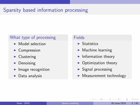
Sparsity based information processing
What type of processing
▶ Model selection
▶ Compression
▶ Clustering
▶ Denoising
▶ Image recognition
▶ Data analysis
Fields▶ Statistics
▶ Machine learning
▶ Information theory
▶ Optimization theory
▶ Signal processing
▶ Measurement technology
Ikeda (ISM) Sparse modeling 26/June/2015 3 / 65

Domestic projects
Figure : MEXT grant-in-aid for scientific research on innovative areas(2013-2018) Initiative for High-Dimensional Data-Driven Science throughDeepening of Sparse Modeling
Ikeda (ISM) Sparse modeling 26/June/2015 4 / 65

Theory of sparse modeling Sparsity and Linear equation
Theory of sparse modelingSparsity and Linear equationSparsity of dataUniqueness of the sparse solutionRelaxed problemNoisy observation
Summary
Ikeda (ISM) Sparse modeling 26/June/2015 5 / 65

Theory of sparse modeling Sparsity and Linear equation
What is sparsity?
A multi-dimensional vector has a lot of zeros.
x = (x1, · · · , xn)T , xi ∈ ℜ.
y is a function of x,
y = f(x)
and the components which contribute to y is small. This is theassumption of sparsity.
▶ A harmonic sound has a lot of zeros in frequency domain.
▶ There are a lot of genes but the ones related to a specific disease aresmall.
▶ Movie is a sequence of images. But the number of pixels changingeach time is not large.
Ikeda (ISM) Sparse modeling 26/June/2015 6 / 65

Theory of sparse modeling Sparsity and Linear equation
Linear equation
y = f(x)
Simple case is a linear equation. Let y = (y1, · · · , ym)T is a function ofn-dimensional real vector x = (x1, · · · , xn)T
yi =∑j
aijxj i = 1, · · · ,m.
by defining A = (aij),
y = Ax.
Assume A is known, and our problem is to estimate x from y.
Ikeda (ISM) Sparse modeling 26/June/2015 7 / 65

Theory of sparse modeling Sparsity and Linear equation
Linear equation: m = n
If m = n and A−1 exists, x = A−1y
y = Ax =
−1 2 −13 −1 2
−1 1 1
x1x2x3
.
When (y1, y2, y3)T is observed, x is computed as follows.
x = A−1y =1
9
3 3 −35 2 1
−2 1 5
y1y2y3
.
Ikeda (ISM) Sparse modeling 26/June/2015 8 / 65

Theory of sparse modeling Sparsity and Linear equation
Linear equation: m < n
If m, the dimension of y is smaller than n, the dimension of x, thesolution becomes under-determined. There are infinitely many solutions xwhich satisfy the equation.
(y1y2
)=
(−1 2 −13 −1 2
)x1x2x3
.
When, y1 = 2, y2 = −1, solving two linear equation brings the followingline.
(x1, x2, x3)T = (−3t, t+ 1, 5t)T .
Any point on this line satisfies the equation.
Ikeda (ISM) Sparse modeling 26/June/2015 9 / 65

Theory of sparse modeling Sparsity and Linear equation
Linear equation: m < n
Suppose x is known to be sparse. The point on the line which makes thesolution sparsest is when t = 0, and the solution is x = (0, 1, 0)T .
Sparse solution
We could solve the equation by assuming the solution is sparse.
Ikeda (ISM) Sparse modeling 26/June/2015 10 / 65

Theory of sparse modeling Sparsity and Linear equation
Single Bit Camera
Figure : A project at Rice university.
Ikeda (ISM) Sparse modeling 26/June/2015 11 / 65

Theory of sparse modeling Sparsity and Linear equation
Single Bit Camera: Problem
Recent digital cameras have a large number of pixels, but this camera hasa single pixel. A single pixel camera uses a lot of micro mirrors forcollecting image.
(a) Image for a camera. (b) A pattern of the micromirrors.
Ikeda (ISM) Sparse modeling 26/June/2015 12 / 65

Theory of sparse modeling Sparsity and Linear equation
Single Bit Camera: Compressed Sensing
x is a image and we would like to observe (sensing) it.Eventually, we want to reconstruct the image from observation.The “single” observation of x is to take the inner product between therow vector of A, that is, a(l) = (al1, · · · , alm), and x. More precisely, asingle observation is equivalent to see the following yl.
yl = a(l)x.
After observing a lot of y1, · · · , yn we want to reconstruct x. The vectory is a collection of yl.
y = Ax.
Donoho (2006). “Compressed sensing,” IEEE tr. IT, 52(4), 1289-1306.
Ikeda (ISM) Sparse modeling 26/June/2015 13 / 65

Theory of sparse modeling Sparsity and Linear equation
Single Bit Camera: How it works.
By repeating observation by changing the patterns of mirrors, we have thefollowing linear equation.
y = Ax.
When A and y are know, we want to compute x.
=
.
Ikeda (ISM) Sparse modeling 26/June/2015 14 / 65

Theory of sparse modeling Sparsity and Linear equation
Single Bit Camera: Simulation
How it works
We set m = 512, n = 1024, and the linear equation is under-determined.x is sparse that only 234 components are positive among 1024components. The sparse solution is shown as follows.
(a) Recorded image. (b) Reconstructed image.
Ikeda (ISM) Sparse modeling 26/June/2015 15 / 65

Theory of sparse modeling Sparsity and Linear equation
Single Bit Camera
Figure : A project at Rice university.
Ikeda (ISM) Sparse modeling 26/June/2015 16 / 65

Theory of sparse modeling Sparsity and Linear equation
Information processing based on sparsity
Simulation works, but we want to know if it works in real. We explain itfrom the following viewpoints.
We explain it from the following topics.
▶ Do the data have sparsity?
▶ Can we obtain the solution if the data have sparsity?
▶ How do we handle noise?
▶ How to compute?
Sparse modeling is a new field that mathematical theory, appliedmathematics, and data analysis are involved.
Ikeda (ISM) Sparse modeling 26/June/2015 17 / 65

Theory of sparse modeling Sparsity of data
Theory of sparse modelingSparsity and Linear equationSparsity of dataUniqueness of the sparse solutionRelaxed problemNoisy observation
Summary
Ikeda (ISM) Sparse modeling 26/June/2015 18 / 65

Theory of sparse modeling Sparsity of data
Sparsity
▶ In information theory, there are some cases where x can begenerated. This is not the case for data analysis.
▶ We want to know if it is reasonable to assume x sparse.
▶ In big data analysis, people sometimes assume data has sparsity.
▶ In genomic data, there are many genes, but only small number ofthem are related to a disease.
▶ Also sound or music data has sparsity.
Ikeda (ISM) Sparse modeling 26/June/2015 19 / 65

Theory of sparse modeling Sparsity of data
Sparsity of sound data
Flute
−1
0
1
s 1(t)
−1
0
1
s 2(t)
0 0.5 1 1.5 2−1
0
1
Time [s]
s 3(t)
(a) Flute sound.
(b) Spectrogram.
Ikeda (ISM) Sparse modeling 26/June/2015 20 / 65

Theory of sparse modeling Sparsity of data
Sparsity of sound data
Acoustic sound
0 0.5 1 1.5 2−1
0
1
Time [s]
s 2(t)
−1
0
1
s 1(t)
(a) Acoustic sound
(b) Spectrogram.
Ikeda (ISM) Sparse modeling 26/June/2015 21 / 65

Theory of sparse modeling Sparsity of data
Sparsity of image data
Wavelet transform
(a) Original image (b) Wavelet coefficients
Ikeda (ISM) Sparse modeling 26/June/2015 22 / 65

Theory of sparse modeling Sparsity of data
Sparsity of image data
Wavelet transform
1 2 3 4 5 6
x 104
−20
−18
−16
−14
−12
−10
−8
−6
−4
−2
0lo
g of
nor
mal
ized
coe
ffs
Figure : Distribution of coefficientsIkeda (ISM) Sparse modeling 26/June/2015 23 / 65

Theory of sparse modeling Sparsity of data
Sparsity of image data
Removing small coefficients (49.86%)
(a) Reconstructed image (b) Wavelet coefficients
Ikeda (ISM) Sparse modeling 26/June/2015 24 / 65

Theory of sparse modeling Sparsity of data
Sparsity of image data
Removing small coefficients (31.92%)
(a) Reconstructed image (b) Wavelet coefficients
Ikeda (ISM) Sparse modeling 26/June/2015 25 / 65

Theory of sparse modeling Sparsity of data
Sparsity of image data
Removing small coefficients (15.45%)
(a) Reconstructed image (b) Wavelet coefficients
Ikeda (ISM) Sparse modeling 26/June/2015 26 / 65

Theory of sparse modeling Sparsity of data
Sparsity of image data
Removing small coefficients (9.03%)
(a) Reconstructed image (b) Wavelet coefficients
Ikeda (ISM) Sparse modeling 26/June/2015 27 / 65

Theory of sparse modeling Sparsity of data
Sparsity of image data
Removing small coefficients (4.03%)
(a) Reconstructed image (b) Wavelet coefficients
Ikeda (ISM) Sparse modeling 26/June/2015 28 / 65

Theory of sparse modeling Sparsity of data
Sparsity of image data
Change the basis
We can change the basis linearly. Fourier and Wavelet transforms in theprevious examples are denoted with a n× n unitary transform Φ as
z = Φx,
where z is a transformed representation.
y = Ax
This problem can be applied even if x is not sparse but z is sparse.Because we can rewrite the problem as the following problem.
y = Ax = AΦ−1z = Bz.
Ikeda (ISM) Sparse modeling 26/June/2015 29 / 65

Theory of sparse modeling Sparsity of data
Sparsity of image data
The number of changing points of the image is small (applying aLaplacian filter and show the square of the output value)
(a) image (b) Filter output
Ikeda (ISM) Sparse modeling 26/June/2015 30 / 65

Theory of sparse modeling Sparsity of data
Sparsity of image data
The number of changing points of the image is small (applying aLaplacian filter and show the square of the output value)
(a) image (b) Filter output
Ikeda (ISM) Sparse modeling 26/June/2015 31 / 65

Theory of sparse modeling Sparsity of data
Sparsity of data
▶ It is not clear what type of sparsity the data have.
▶ In many cases, a sparse representation is obtained after a propertransformation (linear or nonlinear).
▶ It is important to find a proper representation.
Ikeda (ISM) Sparse modeling 26/June/2015 32 / 65

Theory of sparse modeling Uniqueness of the sparse solution
Theory of sparse modelingSparsity and Linear equationSparsity of dataUniqueness of the sparse solutionRelaxed problemNoisy observation
Summary
Ikeda (ISM) Sparse modeling 26/June/2015 33 / 65

Theory of sparse modeling Uniqueness of the sparse solution
Compressed sensing
Consider the following under-determined linear equation
y = Ax
where m < n and y and A are known. If x is sparse and we computed thesparsest solution. Is it unique?This problem depends on the characteristics of the matrix A.
Ikeda (ISM) Sparse modeling 26/June/2015 34 / 65

Theory of sparse modeling Uniqueness of the sparse solution
Norm
The definitions of the norm used in the following analysis
0 norm: ∥x∥ℓ0 = |{x;xi = 0}|1 norm: ∥x∥ℓ1 =
∑i |xi|
2 norm: ∥x∥ℓ2 =(∑
i x2i
)1/2
Definition of norm▶ If ∥x∥ = 0 then x = 0.
▶ ∥ax∥ = |a|∥x∥.▶ ∥x+ y∥ ≤ ∥x∥+ ∥y∥.
To be precise, 0 norm is not a norm. But for convenience, we call it 0norm.
Ikeda (ISM) Sparse modeling 26/June/2015 35 / 65
Theory of sparse modeling Uniqueness of the sparse solution
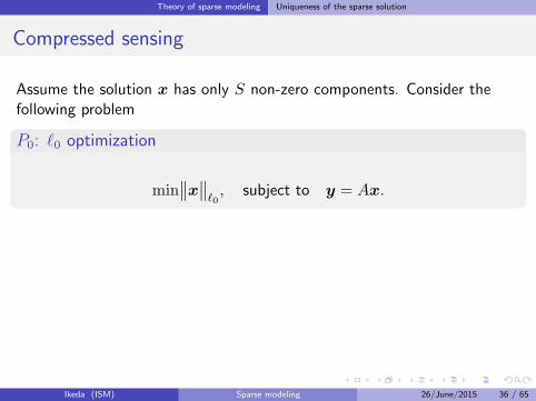
Compressed sensing
Assume the solution x has only S non-zero components. Consider thefollowing problem
P0: ℓ0 optimization
min∥∥x∥∥
ℓ0, subject to y = Ax.
Ikeda (ISM) Sparse modeling 26/June/2015 36 / 65

Theory of sparse modeling Uniqueness of the sparse solution
Compressed sensing
Consider the condition that P0 has a unique solution.
Definition: SPARK
Picking up k column vectors from A, and spark(A) is the minimum kwhere the column vectors become linearly dependent.2 ≤ Spark(A) ≤ m+ 1 holds.
The condition P0 has a unique solution.
A sufficient condition that P0 has a unique solution
If the following holds, x0 is the sparsest solution.
∥x0∥ℓ0 <spark(A)
2.
Ikeda (ISM) Sparse modeling 26/June/2015 37 / 65

Theory of sparse modeling Uniqueness of the sparse solution
RIP (Restricted isometry property)
Another way to characterize the condition where P0 has a unique solutionis to based on a new concept RIP (Restricted isometry property).
Definition: RIP
Assume x has S non-zero component. If there exists a δ satisfies thefollowing inequality, A has RIP(S, δ).
(1− δ)∥∥x∥∥
ℓ2≤
∥∥Ax∥∥ℓ2
≤ (1 + δ)∥∥x∥∥
ℓ2
for all∥∥x∥∥
ℓ0= S
Ikeda (ISM) Sparse modeling 26/June/2015 38 / 65

Theory of sparse modeling Uniqueness of the sparse solution
RIP and P0
ℓ0 recovery
Let S ≥ 1. Suppose A has a RIP and δ2S < 1. If y = Ax holds for an xwith ∥x∥ℓ0 ≤ S, the following problem has a unique solution.
min∥∥x∥∥
ℓ0, subject to y = Ax.
Ikeda (ISM) Sparse modeling 26/June/2015 39 / 65

Theory of sparse modeling Relaxed problem
Theory of sparse modelingSparsity and Linear equationSparsity of dataUniqueness of the sparse solutionRelaxed problemNoisy observation
Summary
Ikeda (ISM) Sparse modeling 26/June/2015 40 / 65

Theory of sparse modeling Relaxed problem
Relax ℓ0 norm optimization
P0: ℓ0 optimization
min∥∥x∥∥
ℓ0, subject to y = Ax.
It is difficult to solve this problem for a large m.
▶ It is not possible to take the derivative of ℓ0 norm.
▶ Computation to check all the combination of x components is hard.
Relax ∥x∥ℓ0 to ∥x∥ℓ1 and consider the following problem.
P1: ℓ1 optimization
min∥∥x∥∥
ℓ1, subject to y = Ax.
∥x∥ℓ1 =∑
i |xi|, and we can apply optimization techniques.
Ikeda (ISM) Sparse modeling 26/June/2015 41 / 65

Theory of sparse modeling Relaxed problem
Relaxing ℓ0 recovery
Suppose x is S-sparse (S ≥ 1). Suppose A has a RIP and δ2S ≤√2− 1.
Then the solutions of the following two problems are the same.
min∥∥x∥∥
ℓ1, subject to y = Ax
min∥∥x∥∥
ℓ0, subject to y = Ax.
If x is sparse and A has a good property, ℓ0 optimization problem can besolved by ℓ1 optimization.
Candes, “The restricted isometry property and its implications forcompressed sensing,” Comptes Rendus Mathematique, 346(9-10),589-592.
Ikeda (ISM) Sparse modeling 26/June/2015 42 / 65
Theory of sparse modeling Relaxed problem
Related researches
▶ ℓ1 recovery problem is theoretically guaranteed to be optimal if x issparse.
▶ These discussions depends on the characteristics of A.
▶ There is a gap between ℓ1 recovery and ℓ0 recovery.
Ikeda (ISM) Sparse modeling 26/June/2015 43 / 65
Theory of sparse modeling Noisy observation
Theory of sparse modelingSparsity and Linear equationSparsity of dataUniqueness of the sparse solutionRelaxed problemNoisy observation
Summary
Ikeda (ISM) Sparse modeling 26/June/2015 44 / 65

Theory of sparse modeling Noisy observation
Regression analysis and LASSO
The observation processed is modeled as follows,
y = Ax
. But in reality, we have noise.
y = Ax+ e
This is a problem of regression. LASSO is proposed in 1996 as a methodto use the sparsity for regression problem.
Ikeda (ISM) Sparse modeling 26/June/2015 45 / 65

Theory of sparse modeling Noisy observation
LASSO
y = Ax+ e
minx
∥y −Ax∥2ℓ2 subject to ∥x∥2ℓ1 ≤ s.
The number of non-zero components of x changes depending on s. As sincreases, the number of non-zero components increases up-to n. As sdecreases, the number of non-zero components decreases to 1.
Equivalent problem with a Lagrange multiplier
minx
[∥y −Ax∥2ℓ2 + λ∥x∥ℓ1
]For each λ ≥ 0 there exists a s ≥ 0 where the both problems becomeequivalent.
Ikeda (ISM) Sparse modeling 26/June/2015 46 / 65

Theory of sparse modeling Noisy observation
LASSO
Likelihood function:
p(y|x;A) = 1
(2πσ2)m/2exp
(− 1
2σ2∥y −Ax∥2ℓ2
)Prior distribution of x:
p(x;µ) =µn
2exp
(−µ∥x∥ℓ1
)
Ikeda (ISM) Sparse modeling 26/June/2015 47 / 65

Theory of sparse modeling Noisy observation
LASSO
Posterior distribution of x:
p(x|y;A,µ) ∝ exp(− 1
2σ2∥y −Ax∥2ℓ2 − µ∥x∥ℓ1
)MAP Estimate:
x = argmaxx
[− 1
2σ2∥y −Ax∥2ℓ2 − µ∥x∥ℓ1
]x = argmin
x
[ 1
2σ2∥y −Ax∥2ℓ2 + µ∥x∥ℓ1
]= argmin
x
[∥y −Ax∥2ℓ2 + λ∥x∥ℓ1
]LASSO is a MAP estimate.
Ikeda (ISM) Sparse modeling 26/June/2015 48 / 65

Theory of sparse modeling Noisy observation
Reference
Compressed sensing
Donoho (2006). “Compressed sensing,” IEEE tr. IT, 52(4), 1289-1306.
LASSO
Tibshirani (1996). “Regression shrinkage and selection via the Lasso,”J. R. Statisti. Soc. B, 58(1), 267-288.
Obourne, Presnell, & Turlach (1999). “On the Lasso and its dual,” J.Comp. and Graph. Stat., 9, 319-337.
Ikeda (ISM) Sparse modeling 26/June/2015 49 / 65

Theory of sparse modeling Noisy observation
A simulated Single Bit Camera
Under-determined linear equation.
=
.
Ikeda (ISM) Sparse modeling 26/June/2015 50 / 65

Theory of sparse modeling Noisy observation
Sparsity of image data
Image is approximately sparse
(a) Original image (b) Wavelet coefficients
Ikeda (ISM) Sparse modeling 26/June/2015 51 / 65

Theory of sparse modeling Noisy observation
Sparsity of image data
This image is not sparse, but is sparse with wavelet basis.Even if x is not sparse, if z is sparse, we can change the representation asfollows,
Ax = AΦ−1z = Bz.
Also, image is roughly sparse but not strictly. Thus we consider theproblem as a noisy regression, and consider it as the following problem,
y = Bz + e.
We use the LASSO.
Ikeda (ISM) Sparse modeling 26/June/2015 52 / 65

Theory of sparse modeling Noisy observation
Sparsity of image data
minz
∥y −Bz∥2ℓ2 + λ∥z∥ℓ1
Solve the problem as LASSO. After solving the problem, z is used torecover the image as x = Φ−1z. We modified λ and solved the problem.
Ikeda (ISM) Sparse modeling 26/June/2015 53 / 65

Theory of sparse modeling Noisy observation
Sparsity of image data
Recovery with LASSO (λ = 10000)
(a) Recovered image (b) Wavelet coefficients
Ikeda (ISM) Sparse modeling 26/June/2015 54 / 65

Theory of sparse modeling Noisy observation
Sparsity of image data
Recovery with LASSO (λ = 100)
(a) Recovered image (b) Wavelet coefficients
Ikeda (ISM) Sparse modeling 26/June/2015 55 / 65

Theory of sparse modeling Noisy observation
Sparsity of image data
Recovery with LASSO (λ = 1)
(a) Recovered image (b) Wavelet coefficients
Ikeda (ISM) Sparse modeling 26/June/2015 56 / 65

Theory of sparse modeling Noisy observation
Sparsity of image data
Image is approximately sparse
(c) Recovered image (d) Wavelet coefficients
Ikeda (ISM) Sparse modeling 26/June/2015 57 / 65

Theory of sparse modeling Noisy observation
Sparsity of image data
Recovery with LASSO (λ = 10000)
(a) Recovered image (b) Wavelet coefficients
Ikeda (ISM) Sparse modeling 26/June/2015 58 / 65

Theory of sparse modeling Noisy observation
Sparsity of image data
Recovery with LASSO (λ = 100)
(a) Recovered image (b) Wavelet coefficients
Ikeda (ISM) Sparse modeling 26/June/2015 59 / 65

Theory of sparse modeling Noisy observation
Sparsity of image data
Recovery with LASSO (λ = 1)
(a) Recovered image (b) Wavelet coefficients
Ikeda (ISM) Sparse modeling 26/June/2015 60 / 65

Theory of sparse modeling Noisy observation
Sparsity of image data
Image is approximately sparse
(a) Recovered image (b) Wavelet coefficients
Ikeda (ISM) Sparse modeling 26/June/2015 61 / 65

Theory of sparse modeling Noisy observation
Sparsity of image data
Recovery with LASSO (λ = 10000)
(a) Recovered image (b) Wavelet coefficients
Ikeda (ISM) Sparse modeling 26/June/2015 62 / 65
Theory of sparse modeling Noisy observation
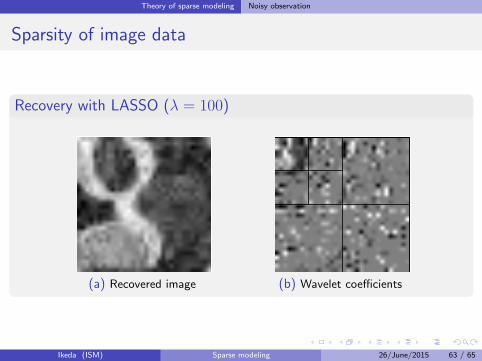
Sparsity of image data
Recovery with LASSO (λ = 100)
(a) Recovered image (b) Wavelet coefficients
Ikeda (ISM) Sparse modeling 26/June/2015 63 / 65

Theory of sparse modeling Noisy observation
Sparsity of image data
Recovery with LASSO (λ = 1)
(a) Recovered image (b) Wavelet coefficients
Ikeda (ISM) Sparse modeling 26/June/2015 64 / 65

Summary
Information processing with sparse modeling
▶ A lot of data have sparsity.
▶ If it is sparse, the optimal solution is unique.
▶ Even if the data is noisy, we can still apply sparsity based methods.
▶ A lot of interesting topics in theory and applications.
Ikeda (ISM) Sparse modeling 26/June/2015 65 / 65