Embed Size (px)
Citation preview

IntroductionNotions of spatial statistics
Spatial econometrics: model specificationEstimation techniques
Diagnostics(Spatially) varying parameters models
Spatial dependence in panel data models
Some notes on Spatial Statistics and SpatialEconometrics
Roberto Basile
Second University of Naples ([email protected])
Roma, 2012
Roberto Basile Spatial Econometrics

IntroductionNotions of spatial statistics
Spatial econometrics: model specificationEstimation techniques
Diagnostics(Spatially) varying parameters models
Spatial dependence in panel data models
Course content
I IntroductionI Notions of spatial statistics
I Spatial econometrics: model specification
I Estimation techniques
I Diagnostics
I (Spatially) varying parameters models
I Spatial dependence in panel data models
Roberto Basile Spatial Econometrics

IntroductionNotions of spatial statistics
Spatial econometrics: model specificationEstimation techniques
Diagnostics(Spatially) varying parameters models
Spatial dependence in panel data models
Spatial data
I Spatial data are those data which combine attribute information(e.g. name of the spatial object, population density, productivity,etc.) with location information (spatial coordinates)(georeferenced data)
I For example, productivity figures are a-spatial unless thelocations for which the data apply are also given
Roberto Basile Spatial Econometrics

IntroductionNotions of spatial statistics
Spatial econometrics: model specificationEstimation techniques
Diagnostics(Spatially) varying parameters models
Spatial dependence in panel data models
Types of spatial data
I Geo-statistical data: continuous spatial variation. Example: air
temperature
I Lattice, regional data (areal or polygonal data):
I the domain is fixed and discreteI spatial locations are often referred to as sitesI we assign to each site one precise spatial coordinate, a
”representative” location (centroid)I regular polygons (lattice data) and irregular polygons (regional
data). For ex. Lombardia and Lazio
I Point data: spatial component = point coordinates x , y. Ex.
Houses, firmsI Line data (arcs): spatial component = ordered set of N points
defining its location x1, y1; x2, y2; ...; xN , yN. Ex. Roads, rivers
Roberto Basile Spatial Econometrics

IntroductionNotions of spatial statistics
Spatial econometrics: model specificationEstimation techniques
Diagnostics(Spatially) varying parameters models
Spatial dependence in panel data models
Special properties of spatial data
I Global spatial autocorrelation or spatial dependence:I Positive: locations close to each other exhibit more similar
values than those further apart. High (low) values aresistematically surrounded by high (low) values
I Negative: high (low) values are sistematically surrounded bylow (high) values
I Local spatial autocorrelation:I If none of the two cases occur sistematically, there is no global
spatial dependence, even though some local spatialautocorrelation may exist
Roberto Basile Spatial Econometrics

IntroductionNotions of spatial statistics
Spatial econometrics: model specificationEstimation techniques
Diagnostics(Spatially) varying parameters models
Spatial dependence in panel data models
Modifiable areal unit problem (MAUP) (polygonal data)
I Scale effects: different results obtained with spatial aggregationat different levels that is with spatial units of different dimensions
I Aggregation or zoning: different results obtained with differentspatial aggregation using spatial units of the same dimension
Roberto Basile Spatial Econometrics

IntroductionNotions of spatial statistics
Spatial econometrics: model specificationEstimation techniques
Diagnostics(Spatially) varying parameters models
Spatial dependence in panel data models
Distance
I Once we know the coordinates of two points, we can computetheir distance
I Arc distance (great-circle distance; takes account of the Earth’scurvature) :
sij = R · arccos
[cos(
90 − xi
)cos(
90 − xj
)+
sin(
90 − xi
)sin(
90 − xj
)cos(
90 − xi
)cos(yj − yi
)]
R is the radius of the earth, x and y are latitudes and longitudes
Roberto Basile Spatial Econometrics

IntroductionNotions of spatial statistics
Spatial econometrics: model specificationEstimation techniques
Diagnostics(Spatially) varying parameters models
Spatial dependence in panel data models
Distance
I It is often more convenient to ignore the curvature of the Earth
I Euclidean distance
d1,2 =
√(x1 − x2)
2 + (y1 − y2)2
I Minkowski metrics (a more general form)
dp1,2 =
[|x1 − x2|p + |y1 − y2|p
]1/p
where p is a constant that can have any value from 1 to ∞
p = 1: Manhattan distance (road distance)p = 2: Euclidean distance (shorter)p can be estimated from a sample of road distances
Roberto Basile Spatial Econometrics

IntroductionNotions of spatial statistics
Spatial econometrics: model specificationEstimation techniques
Diagnostics(Spatially) varying parameters models
Spatial dependence in panel data models
GIS revolution and ESRI shapefiles
I Information on spatial data and coordinates are stored in specialfiles called shapefiles produced through Geographical InformationSystem (GIS) softwares
I A shapefile stores geometry and attribute information for thespatial features in a data set. Features may be points, polygons(i.e. area features), arcs (i.e. sets of connected points) andmulti-points (i.e. clusters of points)
I ESRI (Environmental Systems Research Institute) software is themost famous GIS software used to create shapefiles(http://www.esri.com/)
Roberto Basile Spatial Econometrics

IntroductionNotions of spatial statistics
Spatial econometrics: model specificationEstimation techniques
Diagnostics(Spatially) varying parameters models
Spatial dependence in panel data models
Spatial econometrics
I Spatial econometrics is the collection of econometric tools dealingwith problems of
I spatial dependence
I spatial heterogeneity
I heteroskedasticityI parameter heterogeneity (instability) over space
Roberto Basile Spatial Econometrics

IntroductionNotions of spatial statistics
Spatial econometrics: model specificationEstimation techniques
Diagnostics(Spatially) varying parameters models
Spatial dependence in panel data models
Sources of spatial dependence
I Spatial spillover
I Interregional knowledge flows, trade, factor movements and soon
I Omitted variables
I Unobservable factors (e.g. location amenities) exert aninfluence on the dependent variable and are spatially correlated
I Measurement errors and unobserved heterogeneity
I Administrative boundaries that don’t accurately reflect thenature of underlying DGP
Roberto Basile Spatial Econometrics

IntroductionNotions of spatial statistics
Spatial econometrics: model specificationEstimation techniques
Diagnostics(Spatially) varying parameters models
Spatial dependence in panel data models
Consequences of spatial dependence
I The presence of spatial dependence violates one of the assumptionsof the classical regression model: independence
I This creates a problem in assessing statistical inference: the errorsin the regression model can no longer be assumed to have zerocovariances with each other
I Solutions
I spatial econometric models (spatial lag, spatial error, spatialDurbin models)
I use data at a different spatial scaleI include proxy of non-observablesI include spatial coordinates and/or spatial dummies
Roberto Basile Spatial Econometrics

IntroductionNotions of spatial statistics
Spatial econometrics: model specificationEstimation techniques
Diagnostics(Spatially) varying parameters models
Spatial dependence in panel data models
Spatial heterogeneity
I Lack of spatial stability of the relationships under study:
functional forms and parameters vary with location and are not
homogenous throughout the data setI e.g. classifications of spatial observation: North and South;
Urban and rural areas
I SolutionsI estimate separate models for each group and ask
I are the two relations consistent with the data (Chowtest)?
I is there a trade off between spatial dependence andspatial heterogeneity?
I other methods: varying parameters, random coefficients,GWR, (geo)additive semiparametric models
Roberto Basile Spatial Econometrics

IntroductionNotions of spatial statistics
Spatial econometrics: model specificationEstimation techniques
Diagnostics(Spatially) varying parameters models
Spatial dependence in panel data models
Some Useful Reading Materials
I Anselin L. (1988), Spatial Econometrics, Methods and Models.Boston: Kluwer Academic
I Anselin L. (2003), Spatial Externalities, Spatial Multipliers andSpatial Econometrics, International Regional Science Review, 26,153-166
I Anselin L. (2006), Spatial regression, mimeo
I Fotheringham, A. S., C. Brunsdon, and M. E. Charlton. 2000.Quantitative Geography: Perspectives on Spatial Data Analysis.Thousand Oaks, CA: Sage Publishers
I LeSage J. and Pace R.K. (2009), Introduction to SpatialEconometrics, Taylor & Francis Group, LLC.
Roberto Basile Spatial Econometrics

IntroductionNotions of spatial statistics
Spatial econometrics: model specificationEstimation techniques
Diagnostics(Spatially) varying parameters models
Spatial dependence in panel data models
Software
I GIS :
I GRASS: Geogrpahic Resources Analysis Support SystemI Arc/Info and ArcView GISI maptools (R package)
I Spatial Regression Analysis :
I SpaceStat (gauss routine)I spdep (R package), written by Roger Bivand
(http://crn.r-project.org/)I S+Spatialstats (S-plus)I spatial toolbox (Matlab), written by LeSage-PaceI spatreg (Stata), written by Maurizio PisatiI GeoBugs (http://www.mrc-
bsu.cam.ac.uk/bugs/winbugs/geobugs.shtml)I STARS
Roberto Basile Spatial Econometrics

IntroductionNotions of spatial statistics
Spatial econometrics: model specificationEstimation techniques
Diagnostics(Spatially) varying parameters models
Spatial dependence in panel data models
Motivating Example: Ertur C. and Koch W. (2007)
I The aggregate Cobb-Douglas production function for region i(i = 1, . . . , N) at time t
Yit = AitKτkit L1−τk
it
withAi the aggregate level of technology
Ait = Ωtkφit
N
∏j 6=i
Aρwij
jt
I Ωt = Ω (0) eµt : exogenous technological progress
I kφit : technological externalities among firms within a region
I ∏j 6=i Aρwij
jt : spatial technological externalities (ρ reflects the
degree of spatial externalities)
Roberto Basile Spatial Econometrics

IntroductionNotions of spatial statistics
Spatial econometrics: model specificationEstimation techniques
Diagnostics(Spatially) varying parameters models
Spatial dependence in panel data models
Motivating Example: Ertur C. and Koch W. (2007)
I This model yields a conditional convergence equation which ischaracterized by parameter heterogeneity
γy = D ln y0β + DW ln y0χ + DX ψ + DWX θ + ρDΓW γy + ε
X =[
c ln sk ln (n + g + δ)]
I D = diag(1− e−λi t
)is a diagonal matrix reflecting the
specific effects of the convergence speed in each region
I Γ is a diagonal matrix containing scale heterogeneousparameters reflecting the effects of the speeds of convergencein the neighbouring economies
Roberto Basile Spatial Econometrics

IntroductionNotions of spatial statistics
Spatial econometrics: model specificationEstimation techniques
Diagnostics(Spatially) varying parameters models
Spatial dependence in panel data models
Motivating Example: Ertur and Koch (2007)
I The growth rate is a negative function of the initial level ofper-capita income and a positive function of the initialconditions of its neighbours
I It is also a positive function of reproducible factorsaccumulation rates observed within the region and in itsneighbours,(ln sk , W ln sk), and a negative function of theeffective rate of depreciation within the region and in theneighbours (ln (n + g + δ) , W ln (n + g + δ))
I The last term, W γy , represents the rate of growth in theneighbouring regions
Roberto Basile Spatial Econometrics

IntroductionNotions of spatial statistics
Spatial econometrics: model specificationEstimation techniques
Diagnostics(Spatially) varying parameters models
Spatial dependence in panel data models
Spatial spillover and spatial heterogeneity in long-runregional economic growth: References
I Ertur C. and Koch W. (2011), “A Contribution to the Theory andEmpirics of Shumpeterian Growth with Worldwide Interactions“,Journal of Economic Growth, 16:3, 215-255
I Ertur C. and Koch W. (2007), “Growth, TechnologicalInterdependence and Spatial Externalities: Theory and Evidence“,Journal of Applied Econometrics, vol. 22, pp. 1033-1062
Roberto Basile Spatial Econometrics

IntroductionNotions of spatial statistics
Spatial econometrics: model specificationEstimation techniques
Diagnostics(Spatially) varying parameters models
Spatial dependence in panel data models
Spatial spillover and spatial heterogeneity in long-runregional economic growth: References
I Basile R. (2008), Regional Economic Growth in Europe: aSemiparametric Spatial Dependence Approach, Papers in RegionalScience, Vol. 87, pp. 527-544
I Basile R. (2009), Productivity Polarization Across Regions inEurope: the Role of Nonlinearities and Spatial Dependence,International Regional Science Review, Vol. 32, n. 1, 92-115
I Rey S.J. and J. LeGallo (2009), Spatial Analysis of EconomicConvergence, in T. C. Mills and K. Patterson, Palgrave Handbookof Econometrics Volume II: Applied Econometrics, Pages 1251-1293
Roberto Basile Spatial Econometrics

IntroductionNotions of spatial statistics
Spatial econometrics: model specificationEstimation techniques
Diagnostics(Spatially) varying parameters models
Spatial dependence in panel data models
Course content
I Introduction
I Notions of spatial statistics
I Spatial econometrics: model specification
I Estimation techniques
I Diagnostics
I (Spatially) varying parameters models
I Spatial dependence in panel data models
Roberto Basile Spatial Econometrics

IntroductionNotions of spatial statistics
Spatial econometrics: model specificationEstimation techniques
Diagnostics(Spatially) varying parameters models
Spatial dependence in panel data models
Spatial stochastic processes (random fields)
I Spatial data are thought as drawn from a probability modelspecified as a density function of the form
Φ =
fXS(XS ; θ) , s ∈ S , θ ∈ Θ
I fXS
(XS ; θ) represents the joint probability density function ofan ordered sequence of random variables XS |s ∈ S calledspatial random processes or random fields
I s is an index referring to the spatial location
I It can be either continuous (coordinates of N points in R2
I or discrete (regional data)
Roberto Basile Spatial Econometrics

IntroductionNotions of spatial statistics
Spatial econometrics: model specificationEstimation techniques
Diagnostics(Spatially) varying parameters models
Spatial dependence in panel data models
Topology and spatial interdependence
I In the case of a continuous random field, the topology (i.e. therelationship between spatial features: linkages, adjacencies,inclusion, distance and so on) of the reference space is fullyspecified through the concept of distance
I In the case of discrete random fields, the topology needs to bespecified arbitrarily by the researcher
I In theory, every observation on a variable y at s ∈ S is relatedformally through the function f to the magnitude for the variable inother spatial units in the system:
yi= f(yj)
i = 1, ..., N i 6= j
I This would result in an unidentifiable system, with many moreparameters
(N2 −N
)than observations (N)
Roberto Basile Spatial Econometrics

IntroductionNotions of spatial statistics
Spatial econometrics: model specificationEstimation techniques
Diagnostics(Spatially) varying parameters models
Spatial dependence in panel data models
Solving the identification issue
I We need to impose a structure (parameter restrictions) on therelationships embedded in f , i.e., a particular form for the spatialprocess
I In particular spatial dependence should conform to the fundamentaltheorem of regional science: distance matters (observations thatare near should reflect a greater degree of spatial dependence thanthose more distant from each other). Tobler’s law ofgeography:”Everything is related to everything else, but near thingsare more related than distant things” (spatial friction)
I This suggests that the strength of spatial dependence betweenobservations should decline with the distance between observations,or neighbouring units should exhibit a higher degree of spatialdependence than units located far apart
I Spatial econometrics allows to solve an identification problem
Roberto Basile Spatial Econometrics

IntroductionNotions of spatial statistics
Spatial econometrics: model specificationEstimation techniques
Diagnostics(Spatially) varying parameters models
Spatial dependence in panel data models
Various definitions of neighbourhood
I The very notion of spatial dependence implies the need to determinewhich other units in the spatial system have an influence on theparticular unit under consideration. Formally, this is expressed in thetopological notions of neighbourhood
I Critical cut-off neighbourhood
I k -Nearest neighbours
I Contiguity based neighbourhood
Roberto Basile Spatial Econometrics

IntroductionNotions of spatial statistics
Spatial econometrics: model specificationEstimation techniques
Diagnostics(Spatially) varying parameters models
Spatial dependence in panel data models
Critical cut-off neighbourhood
I Two sites si and sj are said to be neighbours if 0 ≤ dij ≤ d∗ withdij the appropriate distance adopted and d∗ representing thecritical cut-off
I A minimum distance ensures that each location has at least oneneighbour
I If the threshold distance is set to a smaller value, islands will result
Roberto Basile Spatial Econometrics

IntroductionNotions of spatial statistics
Spatial econometrics: model specificationEstimation techniques
Diagnostics(Spatially) varying parameters models
Spatial dependence in panel data models
k-Nearest neighbours
I Two sites si and sj are said to be neighbours if dij ≤ min dik∀k
I This criterion ensures that each observation has exactly the samenumber (k) of neighbours
Roberto Basile Spatial Econometrics

IntroductionNotions of spatial statistics
Spatial econometrics: model specificationEstimation techniques
Diagnostics(Spatially) varying parameters models
Spatial dependence in panel data models
Contiguity based neighbourhood
I Two sites si and sj are said to be neighbours if they share acommon boundary
I Rook-contiguity : Regions share a common edge (exclusion ofonly ‘corner touching’)
I Bishop-contiguity : Consider only touching corners
I Queen-contiguity : Consider either touching corners ortouching edges
Roberto Basile Spatial Econometrics

IntroductionNotions of spatial statistics
Spatial econometrics: model specificationEstimation techniques
Diagnostics(Spatially) varying parameters models
Spatial dependence in panel data models
Spatial weight matrices
I Ones neighbouring regions or points have been identified, thereremains the problem of how to weight them in any calculation
I An option is to not give any weight. In such a case we can build abinary spatial weights matrix
Roberto Basile Spatial Econometrics

IntroductionNotions of spatial statistics
Spatial econometrics: model specificationEstimation techniques
Diagnostics(Spatially) varying parameters models
Spatial dependence in panel data models
Binary spatial weights matrix
I N by N matrix W , with elements wij measuring the associationor neighbourhood between regions i and j
I wij = 1 for i and j neighbours
I wij = 0 otherwise
0 1 0 01 0 1 00 1 0 10 0 1 0
W
=
Roberto Basile Spatial Econometrics

IntroductionNotions of spatial statistics
Spatial econometrics: model specificationEstimation techniques
Diagnostics(Spatially) varying parameters models
Spatial dependence in panel data models
Binary spatial weights matrix-Row standardization
w sij = wij/ ∑j wij s.t. ∑j w s
ij = 1
0 1 0 01 2 0 1 2 00 1 2 0 1 20 0 1 0
W
=
Roberto Basile Spatial Econometrics

IntroductionNotions of spatial statistics
Spatial econometrics: model specificationEstimation techniques
Diagnostics(Spatially) varying parameters models
Spatial dependence in panel data models
Binary spatial weights matrix
I k-nearest-neighbours weights matrix : wij = 1 if thegeographical center of region j is one of the nearest k to thecenter of region i ; otherwise wij = 0 . This weights matrix is notsymmetric
I Contiguity weights matrix : wij = 1 if regions i and j have acommon boundary; otherwise wij = 0
I Distance-based binary weights matrix : wij = 1 if the (great-circleor Euclidean) distance between regions i and j is less than athreshold cut-off distance, otherwise wij = 0
Roberto Basile Spatial Econometrics

IntroductionNotions of spatial statistics
Spatial econometrics: model specificationEstimation techniques
Diagnostics(Spatially) varying parameters models
Spatial dependence in panel data models
Cliff and Ord (1981)
I Cliff and Ord (1981) suggest to use the length of the commonborder between contiguous regions, weighted by a distance function:
wij =[dij]−a [
βij
]bd distance between (centroids of) spatial units i and j
β share of common boundary between i and j (reflects theintensity of the relationship)
a and b parameters estimated from data or chosen a priori
wij =[dij]−a
: gravitational-type weighting
Roberto Basile Spatial Econometrics

IntroductionNotions of spatial statistics
Spatial econometrics: model specificationEstimation techniques
Diagnostics(Spatially) varying parameters models
Spatial dependence in panel data models
Alternative notions of proximity
I Perceived distance or proximity
I Road distance or travel distance
I Non-geographical proximity criteriainstitutionaltechnologicalrelationalsocialother types of proximity: use of interaction data (migrationflows, traffic or telephone calls)
Roberto Basile Spatial Econometrics

IntroductionNotions of spatial statistics
Spatial econometrics: model specificationEstimation techniques
Diagnostics(Spatially) varying parameters models
Spatial dependence in panel data models
Higher Orders of Contiguity (‘neigbours of neigbours’)
I Pure higher order contiguity : does not include locations thatwhere also contiguous of lower order (textbook definition)
I Cumulative order contiguity : includes all lower order neighbours aswell
Roberto Basile Spatial Econometrics

IntroductionNotions of spatial statistics
Spatial econometrics: model specificationEstimation techniques
Diagnostics(Spatially) varying parameters models
Spatial dependence in panel data models
Spatial lag operator
I The spatial lag operator works to produce a weighted average of theneighbouring observations
+ = = = +
∑1 2
2 1 3
3 2 4
4 3
0 1 0 01 2 0 1 2 0 1 2 1 20 1 2 0 1 2 1 2 1 20 0 1 0
ij
s sj
j
y yy y y
w yy y yy y
W y
W s = raw standardized matrix
Roberto Basile Spatial Econometrics

IntroductionNotions of spatial statistics
Spatial econometrics: model specificationEstimation techniques
Diagnostics(Spatially) varying parameters models
Spatial dependence in panel data models
Spatial autocorrelation statistics
I Null Hypothesis : no spatial autocorrelation
I Spatial randomness (vs. spatial clustering)I Values observed at a location do not depend on values
observed at neighbouring locationsI Observed spatial pattern of values is equally likely as any other
spatial patternI The location of values may be altered (spatial permutation)
without affecting the information content of the data
I Alternative Hypotheses
I Positive spatial autocorrelation: like values tend to cluster inspace / Neighbours are similar
I Negative spatial autocorrelation: Neighbours are dissimilar
Roberto Basile Spatial Econometrics

IntroductionNotions of spatial statistics
Spatial econometrics: model specificationEstimation techniques
Diagnostics(Spatially) varying parameters models
Spatial dependence in panel data models
Global spatial autocorrelation
I Moran’s (1950) I
I Geary’s (1954) c
I Getis and Ord’s (1992) G
I We compute only one test statistic which synthesizes theinformation about the degree of spatial dependence
Roberto Basile Spatial Econometrics

IntroductionNotions of spatial statistics
Spatial econometrics: model specificationEstimation techniques
Diagnostics(Spatially) varying parameters models
Spatial dependence in panel data models
Local spatial autocorrelation
I Local Moran’s I (Anselin, 1995)
I Local Geary’s c (Anselin, 1995)
I Local G ∗ (Getis and Ord, 1995)
I we compute a test statistic for each point in space. The aim isto learn about each individual datum by relating it in someway to the values observed at neighbouring locations oftenusing maps to visualize the output
Roberto Basile Spatial Econometrics

IntroductionNotions of spatial statistics
Spatial econometrics: model specificationEstimation techniques
Diagnostics(Spatially) varying parameters models
Spatial dependence in panel data models
Global Moran’s (1950) I spatial autocorrelation statistic
I =
(N
∑i ∑j wij
)(∑i ∑j wij (xi − x) (xj − x)
∑i (xi − x)2
)
I It measures the extent to which high values are generally locatednear to other high values and low values are generally located nearto other low values
I Where the data are distributed such that high and low values aregenerally located near each other, the data are said to exhibitnegative spatial autocorrelation
I When there is no autocorrelation present, the expectationofI is−1/(N − 1)
I When there is a maximum autocorrelation present I will approach 1
Roberto Basile Spatial Econometrics

IntroductionNotions of spatial statistics
Spatial econometrics: model specificationEstimation techniques
Diagnostics(Spatially) varying parameters models
Spatial dependence in panel data models
Geary’s (1954) c
c =
((N − 1)
2 ∑i ∑j wij
)(∑i ∑j wij (xi − xj )
2
∑i (xi − x)2
)
I When there is no autocorrelation present, the expectation of c is 1
I When there is a maximum autocorrelation present c will be near 0
I c is more sensitive to |xi − xj |, while I is more sensitive to extreme
x -values
I However, in general, the results of analyses using c and using I will
provide bradly the same conclusions
Roberto Basile Spatial Econometrics

IntroductionNotions of spatial statistics
Spatial econometrics: model specificationEstimation techniques
Diagnostics(Spatially) varying parameters models
Spatial dependence in panel data models
Classical statistical inference
I Classical statistical inference operates as follows:
I A null hypothesis is stated, such as ‘the population fromwhich this sample was drawn has a parameter value of zero’.Ex.: H0 : θ = θ0
I Then, a statistic, such as a t-statistic or a z-score, iscalculated from the sample data set. Ex.: Z = θ−θ0√
Var (θ)I This statistic is compared with a theoretical distribution with
known probability properties (e.g. the student-t or thestandard normal distribution). On the basis of this comparison,we can reject or accept the null hypothesis according to somea priori and arbitrary cut-off point
Roberto Basile Spatial Econometrics

IntroductionNotions of spatial statistics
Spatial econometrics: model specificationEstimation techniques
Diagnostics(Spatially) varying parameters models
Spatial dependence in panel data models
Classical statistical inference
I In our case, for example, we test whether the magnitude of the
observed value of I Moran is unusual in the absence of spatial
aggregation and reject the hypothesis of no spatial autocorrelation if
the I Moran statistic is sufficiently extreme. So we compute a Zscore and compare it with the normal distribution
Roberto Basile Spatial Econometrics

IntroductionNotions of spatial statistics
Spatial econometrics: model specificationEstimation techniques
Diagnostics(Spatially) varying parameters models
Spatial dependence in panel data models
Inference on Moran’s I based on approximate tests
I The expected value and variance of the Moran I for samples of size
N could be calculated according to the assumed pattern of spatial
data distribution and the normal test for the null hypothesis of no
spatial autocorrelation between observed values over the N locations
can be conducted based on the standardized Moran I
I The expected value of I is −1/(N − 1)
Roberto Basile Spatial Econometrics

IntroductionNotions of spatial statistics
Spatial econometrics: model specificationEstimation techniques
Diagnostics(Spatially) varying parameters models
Spatial dependence in panel data models
Inference on Moran’s I based on approximate tests
I Two theoretical formulae to calculate the variance of I
- Normal approximation: each observed value of the attribute x
is drawn independently from a normal distribution
- Random approximation: the process producing the observed
data pattern is random and the observed pattern is just one out of
the many possible permutations of N data values distributed in N
spatial units
Roberto Basile Spatial Econometrics

IntroductionNotions of spatial statistics
Spatial econometrics: model specificationEstimation techniques
Diagnostics(Spatially) varying parameters models
Spatial dependence in panel data models
Inference on Moran’s I under normal approximation
E (I ) = − 1N−1 var (I ) =
N2S1+NS2+3(∑i ∑j wij)2
(∑i ∑j wij)2(N2−1)
S1 = 12 ∑i ∑j (wij + wji )
2 S2 = ∑i
(∑j wij + ∑j wji
)2
I Under the normal approximation, var (I ) only depends on the
spatial weights and not on the variable under consideration
I Cliff and Ord (1981) find that with a large number of places, the
normal approximation is usually accurate and is of practical value in
testing the significance of departure from the null hypothesis
Roberto Basile Spatial Econometrics

IntroductionNotions of spatial statistics
Spatial econometrics: model specificationEstimation techniques
Diagnostics(Spatially) varying parameters models
Spatial dependence in panel data models
Inference on Moran’s I under randomization
E (I ) = − 1N−1 Var (I ) = NS4−S3S5
(N−1)(N−2)(N−3)(∑i ∑j wij)2
S1 = 12 ∑i ∑j (wij + wji )
2 S2 = ∑i
(∑j wij + ∑j wji
)2
S3 = N−1 ∑i (xi−x)4
(N−1 ∑i (xi−x)2)
2
S4 =(N2 − 3N + 3
)S1 −NS2 + 3
(∑i ∑j wij
)2
S5 = S1 − 2NS1 + 6(∑i ∑j wij
)2
Roberto Basile Spatial Econometrics

IntroductionNotions of spatial statistics
Spatial econometrics: model specificationEstimation techniques
Diagnostics(Spatially) varying parameters models
Spatial dependence in panel data models
Inference on Moran’s I
I The distribution of I is asymptotically normal under either
assumption (normality or randomization); in other words, as long as
N is ‘large’, the following standardized statistic can be calculated
Z =I − E (I )√
Var (I )∼ N (0, 1)
and reference made to normal probability tables
I The questions raised by this procedure are ‘how large does N have
to be?’ and ‘how well does the assumption of asymptotic normality
hold even if N is large?’
Roberto Basile Spatial Econometrics

IntroductionNotions of spatial statistics
Spatial econometrics: model specificationEstimation techniques
Diagnostics(Spatially) varying parameters models
Spatial dependence in panel data models
Interpretation of Moran’s I
I E (I ) = expected value of Moran’s I (i.e. the value that would be
obtained if there were no spatial pattern to the data)
I Positive spatial autocorrelation: I > E (I ) and z > 0, there
is spatial clustering of high and low values: similar values cluster
together. If z exceeds the upper one-tailed 5% point of the
standardized normal distribution, we conclude that there is
significant positive spatial autocorrelation
I Negative spatial autocorrelation: I < E (I ) and z < 0, there
is a checherboard patter, “competition”
Roberto Basile Spatial Econometrics

IntroductionNotions of spatial statistics
Spatial econometrics: model specificationEstimation techniques
Diagnostics(Spatially) varying parameters models
Spatial dependence in panel data models
Interpretation of Moran’s I
I In practice, values greater than 2 or smaller than -2 indicate spatial
autocorrelation that is significant at the 5% level
I If only positive spatial autocorrelation is conceivable, we carry out a
one-sided significance test
Roberto Basile Spatial Econometrics

IntroductionNotions of spatial statistics
Spatial econometrics: model specificationEstimation techniques
Diagnostics(Spatially) varying parameters models
Spatial dependence in panel data models
Inference on Geary’s c under normal approximation
E (c) = 1 Var (c) =(2S1+S2)(N−1)−4(∑i ∑j wij)
2
2(N+1)(∑i ∑j wij)2
S1 = 12 ∑i ∑j (wij + wji )
2
S2 = ∑i
(∑j wij + ∑j wji
)2
Z =c − E (c)√
Var (c)
Roberto Basile Spatial Econometrics

IntroductionNotions of spatial statistics
Spatial econometrics: model specificationEstimation techniques
Diagnostics(Spatially) varying parameters models
Spatial dependence in panel data models
Inference on Geary’s c under randomization
E (c) = 1Var (c) = (N − 1) S1
[N2 − 3N + 3− (N − 1) S3
]− (1/4) (N − 1) S2
[N2 + 3N − 6−
(N2 −N + 2
)S3
]+(∑i ∑j wij
)2[
N2 − 3− (N − 1)2 S3
]/
N (N − 1) (N − 2)(∑i ∑j wij
)S3 = N−1 ∑i (xi−x)
4
(N−1 ∑i (xi−x)2)
2
Roberto Basile Spatial Econometrics

IntroductionNotions of spatial statistics
Spatial econometrics: model specificationEstimation techniques
Diagnostics(Spatially) varying parameters models
Spatial dependence in panel data models
Interpretation of Geary’s c
I The value of Geary’s c lies between 0 and 2. 1 means no spatial
autocorrelation. Smaller (larger) than 1 means negative (positive)
spatial autocorrelation
I Positive spatial autocorrelation: 0 < c < 1 and z < 0, there
is spatial clustering of high and low values
I Negative spatial autocorrelation: 1 < c < 2 and z > 0,
there is a checherboard patter, “competition”
Roberto Basile Spatial Econometrics

IntroductionNotions of spatial statistics
Spatial econometrics: model specificationEstimation techniques
Diagnostics(Spatially) varying parameters models
Spatial dependence in panel data models
Values of I and c
I When I approaches +1: strong positive spatial autocorrelation
I When I approaches -1: strong negative spatial autocorrelation
I When I approaches 0: no spatial autocorrelation
I When c approaches 0: strong positive spatial autocorrelation
I When c approaches 2: strong negative spatial autocorrelation
I When c approaches 1: no spatial autocorrelation
Roberto Basile Spatial Econometrics

IntroductionNotions of spatial statistics
Spatial econometrics: model specificationEstimation techniques
Diagnostics(Spatially) varying parameters models
Spatial dependence in panel data models
Scale effects
I Measures of spatial autocorrelation are scale dependent. For
example, clustered point patterns can aggregate to either positively
or negatively autocorrelated areal patterns
I This is an example of the MAUP
Roberto Basile Spatial Econometrics

IntroductionNotions of spatial statistics
Spatial econometrics: model specificationEstimation techniques
Diagnostics(Spatially) varying parameters models
Spatial dependence in panel data models
Global G
I Getis. A, Ord, J. K. (1992), The analysis of spatial association by
use of distance statistics, Geographical Analysis, 24, p. 195
I measures the way in which values of an attribute are clustered in
space
G (d) = ∑i
∑j
wij (d) xixj/ ∑i
∑j
xixj
I standardized G statistic, Z (G ) = G−E (G )√Var (G )
I Z (G ) > 0 the spatial pattern is dominated by clusters of highvalues
I Z (G ) < 0 the spatial pattern are dominated by clusters of lowvalues
Roberto Basile Spatial Econometrics

IntroductionNotions of spatial statistics
Spatial econometrics: model specificationEstimation techniques
Diagnostics(Spatially) varying parameters models
Spatial dependence in panel data models
Limit of the classical statistical inference
I Whichever approach we take to making inference using the classical
approach, it is necessary to be able to assume some form of
theoretical distribution for the test statistic
I For some statistics, such as the sample mean and OLS parameter
estimates, the theoretical distributions are well known and can, in
most circumstances, be used with confidence that the assumptions
concerning the distributions are met
Roberto Basile Spatial Econometrics

IntroductionNotions of spatial statistics
Spatial econometrics: model specificationEstimation techniques
Diagnostics(Spatially) varying parameters models
Spatial dependence in panel data models
Limit of the classical statistical inference
I However, for some statistics, either there is no known theoretical
distribution against which to compare the observed value, or, where
the distribution is known, the assumptions underlying the use of
that particular distributions are unlikely to be met. Both of these
circumstances are common in the analysis of spatial data and here
the construction of experimental distributions becomes especially
useful
Roberto Basile Spatial Econometrics

IntroductionNotions of spatial statistics
Spatial econometrics: model specificationEstimation techniques
Diagnostics(Spatially) varying parameters models
Spatial dependence in panel data models
Experimental distributions
I The central idea in the use of experimental distributions for
statistical inference is that the sampled data can yield a better
estimate of the underlying distribution of the calculated statistic
than making perhaps unrealistic assumptions about the population
I The sample data are re-sampled in some way to create a set of
samples, each of which yields an estimate of a particular statistic. If
this is done many times, the frequency distribution of the statistic
forms the experimental distribution against which the value from
the original sample can be compared. Consequently, the
experimental distribution can be constructed for any statistic, even
if the theoretical distribution is unknown
Roberto Basile Spatial Econometrics

IntroductionNotions of spatial statistics
Spatial econometrics: model specificationEstimation techniques
Diagnostics(Spatially) varying parameters models
Spatial dependence in panel data models
Experimental distribution in spatial statistics:“randomisation”
I Assign values to locations by means of a random permutation. With
N locations, N !different random permutations of xi values (and
thus N ! maps) could be produced
I Derive the spatial autocorrelation statistic for each of these maps.
Thus, we have a reference distribution against which to evaluate the
one we actually observed
Roberto Basile Spatial Econometrics

IntroductionNotions of spatial statistics
Spatial econometrics: model specificationEstimation techniques
Diagnostics(Spatially) varying parameters models
Spatial dependence in panel data models
Experimental distribution in spatial statistics:“randomisation”
I If observed spatial autocorrelation statistic lies in a tail of the
sampling distribution, then we would have a statistical basis for
arguing that the observed spatial distribution of the variable
probably do not come from a random allocation process. We
interpret this fact as suggesting the existence of significant spatial
autocorrelation in the dataI In general, N ! random permutations of xi values could be produced.
A close approximation to the reference set distribution can be
obtained by sampling from the N ! permutation (the Monte Carlo
approach). This method is recommended whenever full
randomization tests appear desirable but computationally
cumbersomeRoberto Basile Spatial Econometrics

IntroductionNotions of spatial statistics
Spatial econometrics: model specificationEstimation techniques
Diagnostics(Spatially) varying parameters models
Spatial dependence in panel data models
Moran’s I test: a Monte Carlo experiment
I Four steps:1) calculate I for the observed distribution of x and call this I ∗
2) randomly reassign the N data values across the N spatial units3) calculate I for the new spatial distribution of x and store4) repeat steps 2 and 3 many times (at least 99 time and preferably999 time)
I This will produce an experimental distribution for I against whichthe value of I ∗ can be assessed. The proportion of values in theexperimental distribution which equal or exceed I ∗ yields anestimate of the probability that a value of Moran’s I as high as I ∗
could have risen by chance
Roberto Basile Spatial Econometrics

IntroductionNotions of spatial statistics
Spatial econometrics: model specificationEstimation techniques
Diagnostics(Spatially) varying parameters models
Spatial dependence in panel data models
Moran’s I test: a Monte Carlo experiment
I For example, if the observed value of I = 0.21 is exceeded by 14 ofthe 99 random permutations, we conclude that the chance ofobtaining values of I larger than 0.21 is 14%, which is not a smallprobability and, thus, we conclude that the data are not significantlyspatially auto-correlated
Roberto Basile Spatial Econometrics

IntroductionNotions of spatial statistics
Spatial econometrics: model specificationEstimation techniques
Diagnostics(Spatially) varying parameters models
Spatial dependence in panel data models
Local spatial autocorrelation statistics
I Global spatial autocorrelation statistics are based on the assumption
of stationarity or structural stability over space, which is often
unrealistic in many contexts. Spatial association can be detected
using local spatial autocorrelation indices which allow for local
instabilities in overall spatial association
I The aim is to learn more about each individual datum by relating it
in some way to the values observed at neighbouring locations often
by using visualization of the resulting maps as a direct analytical
procedure
Roberto Basile Spatial Econometrics

IntroductionNotions of spatial statistics
Spatial econometrics: model specificationEstimation techniques
Diagnostics(Spatially) varying parameters models
Spatial dependence in panel data models
Local Moran’s I
I Anselin (1995) has shown that Moran’s I spatial autocorrelationcoefficients can be decomposed into local values. The local form ofMoran’s I is a product of the zone value and the average in thesurrounding zones:
Ii (d) =(xi−x)∑j wij(xj−x)
∑i (xi−x)2/N
E (Ii ) = −wi ./ (N − 1) wi . = ∑j wij j 6= i
Var (Ii ) = w2i .V
where V is the variance of I under randomization
Roberto Basile Spatial Econometrics

IntroductionNotions of spatial statistics
Spatial econometrics: model specificationEstimation techniques
Diagnostics(Spatially) varying parameters models
Spatial dependence in panel data models
Local Moran’s I
Anselin, L. 1995. Local indicators of spatial association,Geographical Analysis, 27, 93–115
Anselin, L. 1996. The Moran scatterplot as an ESDA toolto assess local instability in spatial association. pp. 111–125 inM. M. Fischer, H. J. Scholten and D. Unwin (eds) Spatialanalytical perspectives on GIS, London, Taylor and Francis
Roberto Basile Spatial Econometrics

IntroductionNotions of spatial statistics
Spatial econometrics: model specificationEstimation techniques
Diagnostics(Spatially) varying parameters models
Spatial dependence in panel data models
Moran scatterplot
I Plot of Wx against x. A positive relation indicate positive spatialautocorrelation. The Moran scatterplot can be used to depictspatial outliers, defined as zones having very different values of anattribute from their neighbour
I Four quadrants:high-high, low-low = spatial clusterhigh-low, low-high = spatial outliers
I Moran’s ISlope of linear scatterplot smoother
I Identify Hot Spots:I Significant local clusters in the absence of global
autocorrelation (or some complication in the presence of globalautocorrelation, i.e. extra heterogeneity)
I Significant local outliers (high surrounded by low and viceversa)
I Indicate local instability (local deviations from global patternof spatial autocorrelation)
Roberto Basile Spatial Econometrics

IntroductionNotions of spatial statistics
Spatial econometrics: model specificationEstimation techniques
Diagnostics(Spatially) varying parameters models
Spatial dependence in panel data models
Local G
I Indicates the extent to which a location is surrounded to a distanced by a cluster of high or low values
I There are two variants of this localized statistic (G and G*)depending on whether or not the unit i around which the clusteringis measured is included in the calculation
I Unfortunately there is no theory to guide the use of which statisticto use in any particular situation although the difference betweenthe two will typically be very small in most situations where thereare large numbers of spatial units
Roberto Basile Spatial Econometrics

IntroductionNotions of spatial statistics
Spatial econometrics: model specificationEstimation techniques
Diagnostics(Spatially) varying parameters models
Spatial dependence in panel data models
Local G
I For the situation where i is not included in the calculation
Gi=∑j wijxj
∑j xjj 6= i
I If high values of x tend to be clustered around i, Gi will be high; if
low values of x tend to cluster around i then Gi will be low. No
distict clustering of high or low values of x around i will produce
intermediate values of Gi
Roberto Basile Spatial Econometrics

IntroductionNotions of spatial statistics
Spatial econometrics: model specificationEstimation techniques
Diagnostics(Spatially) varying parameters models
Spatial dependence in panel data models
Local G
I For the situation when i is included in the calculation, then the
above formulae simplify to
G ∗i =∑j wijxj
∑j xj∀i
where wii must not equal zero
Roberto Basile Spatial Econometrics

IntroductionNotions of spatial statistics
Spatial econometrics: model specificationEstimation techniques
Diagnostics(Spatially) varying parameters models
Spatial dependence in panel data models
Local G
I The Gi and the G∗i statistics are normally distributed
E (Gi ) = wi ./ (N − 1) wi . = ∑j
wij j 6= i
Var (Gi ) = wi . (N − 1− wi .) s2i / (N − 1)2 (N − 2) x2
i
E (G ∗i ) = w∗i ./N w∗i . = ∑j
wij ∀i
Var (G ∗i ) = wi . (N − w∗i .) s2i /N2 (N − 1) x2
i
where s2i is the sample estimate of the variance of x, again
excluding the value i
Roberto Basile Spatial Econometrics

IntroductionNotions of spatial statistics
Spatial econometrics: model specificationEstimation techniques
Diagnostics(Spatially) varying parameters models
Spatial dependence in panel data models
Local G
I A standard variate can be defined as
Z (Gi ) = [Gi − E (Gi )] / [Var (Gi )]1/2
Roberto Basile Spatial Econometrics

IntroductionNotions of spatial statistics
Spatial econometrics: model specificationEstimation techniques
Diagnostics(Spatially) varying parameters models
Spatial dependence in panel data models
The Critical Distance
I The G ∗i values are computed around each observation as distanceincreases
I When the absolute values fail to rise, the cluster diameter isreached. This is the critical distance dc
I Spatial association weakens beyond dc
Roberto Basile Spatial Econometrics

IntroductionNotions of spatial statistics
Spatial econometrics: model specificationEstimation techniques
Diagnostics(Spatially) varying parameters models
Spatial dependence in panel data models
References on Local G
Ord, J. K. and Getis, A. 1995 Local spatial autocorrelationstatistics: distributional issues and an application.Geographical Analysis, 27, 286–306
Getis, A. and Ord, J. K. 1996 Local spatial statistics: anoverview. In P. Longley and M. Batty (eds) Spatial analysis:modelling in a GIS environment (Cambridge: GeoinformationInternational), 261–277
Roberto Basile Spatial Econometrics

IntroductionNotions of spatial statistics
Spatial econometrics: model specificationEstimation techniques
Diagnostics(Spatially) varying parameters models
Spatial dependence in panel data models
Bonferroni correction
I The distribution of a generic LISA depends of the distribution forthe correspondent global statistic
I Bonferroni correction: if an experimenter is testing N independenthypotheses on a set of data, then the statistical significance levelthat should be used for each hypothesis separately is 1/N timeswhat it would be if only one hypothesis were tested
I For example, when testing two hypotheses, instead of a valueof α of 0.05, one would use a stricter a value of 0.025
Roberto Basile Spatial Econometrics

IntroductionNotions of spatial statistics
Spatial econometrics: model specificationEstimation techniques
Diagnostics(Spatially) varying parameters models
Spatial dependence in panel data models
Spatial stationarity, ergodicity and isotropy
Spatial stationarity
I Since spatial data are not independent, we must make some
assumptions on the ‘stationarity’ of the process. In time series, this
means that the joined distributions are the same at any point in
time. In the spatial context, this is to say that the joined
distributions are the same throughout space, regardless of absolute
positions, depending only on relative positions
Strict stationarity:
I A random field XS |s ∈ S is stationary (in a strict sense) if the
DGP of the realizations remains constant over space, that is if
∀s ∈ S the joint pdf f (XS , s ∈ S) does not change when the
subset is shifted in the spaceRoberto Basile Spatial Econometrics

IntroductionNotions of spatial statistics
Spatial econometrics: model specificationEstimation techniques
Diagnostics(Spatially) varying parameters models
Spatial dependence in panel data models
Rotation and translation
I If a random field remains unchanged in terms of its joint pdf after a
translation, it is said to be stationary under translations, or
homogenous
I If a random field remains unchanged in terms of its joint pdf after arotation, it is said to be stationary under rotation around a fixedpoint, or isotropic, which implies that the dependence structuredoes not change systematically along different directions
I A consequence of strict stationarity is that all univariate momentsand all mixed moments of any order do not vary when the referencespace is modified
Roberto Basile Spatial Econometrics

IntroductionNotions of spatial statistics
Spatial econometrics: model specificationEstimation techniques
Diagnostics(Spatially) varying parameters models
Spatial dependence in panel data models
Weak stationarity
I A random field XS |s ∈ S is said to be stationary of order k if
∀s ∈ S the moments of order k of its joint pdf f (XS , s ∈ S) do
not change when the subset is subject to translations or rotations
I a r.f. is stationary of order 1 if
E (Xs) = E (Xs+δ) = µ ∀s ∈ S
I a r.f. is stationary of order 2 if
E (Xs) = E (Xs+δ) = µ ∀s ∈ S
E (Xs)2 = E (Xs+δ)
2 = σ2 ∀s ∈ S
E (Xsi , Xsj ) = γ (dij ) ∀si , sj ∈ S(the covariance depends only on the distance)
Roberto Basile Spatial Econometrics

IntroductionNotions of spatial statistics
Spatial econometrics: model specificationEstimation techniques
Diagnostics(Spatially) varying parameters models
Spatial dependence in panel data models
Ergodicity
I A random field XS |s ∈ Swhich is stationary up to the second
order is said to be ergodic if
limdij→∞
1∆ ∑dij
ρ (si , sj ) = 0
I This implies convergence in probability:
N−1∑i
xip→ µ
N−1 ∑i
(xi − µ)2 p→ σ2
1N(N−1)∑
i∑j(xi − µ) (xj − µ)
p→ γ (dij )
Roberto Basile Spatial Econometrics

IntroductionNotions of spatial statistics
Spatial econometrics: model specificationEstimation techniques
Diagnostics(Spatially) varying parameters models
Spatial dependence in panel data models
Ergodicity
I Correlograms are graphs (or tables) showing how autocorrelation
changes with distance
I The typical behavior of many spatial phenomena produces a
correlogram that displays values that diminish rapidly towards zero
as the inter-point distance rapidly increases, thus, giving some
empirical substantiation to the first law of geography (Tobler, 1970)
Roberto Basile Spatial Econometrics

IntroductionNotions of spatial statistics
Spatial econometrics: model specificationEstimation techniques
Diagnostics(Spatially) varying parameters models
Spatial dependence in panel data models
Exploratory spatial data analysis
I Exploratory data analysis (EDA) consists of a set of techniques to
explore data in order to suggest hypotheses or to examine the
presence of outliers (Tukey, 1950)
I We recognize the need to visualize data and trends prior to
performing some type of formal analysis
I Other use: examine model accuracy and robustness (e.g. mapping
the residuals from a model in order to provide improved
understanding of why the model fails to replicate the data exactly)
Roberto Basile Spatial Econometrics

IntroductionNotions of spatial statistics
Spatial econometrics: model specificationEstimation techniques
Diagnostics(Spatially) varying parameters models
Spatial dependence in panel data models
Empirical questions of the EDA
I Are there variables having unusually high or low values?
I What distributions do the variables follow?
I Do observations fall into a number of distinct groups?
I What associations exist between variables?
Roberto Basile Spatial Econometrics

IntroductionNotions of spatial statistics
Spatial econometrics: model specificationEstimation techniques
Diagnostics(Spatially) varying parameters models
Spatial dependence in panel data models
Univariate ESDA
I Position indices: mean (m), median (Q2), first and third quartiles
(Q1 and Q3)I Variability indices: standard deviation (s) (spatially corrected),
coefficient of variation (CV=s/m), interquartile range(Q3-Q1),
min-maxI Concentration indices (spatially corrected): Gini and TheilI Skewness and kurtosisI Global indices of spatial auocorrelation: Moran’s I, Getis and Ord,
. . .I Local indices of spatial autocorrelation: local Moran’s I, local G∗
I Visual univariate ESDA: histogram, univariate density, boxplot,
Choroplet maps, Moran’s scatterplot, maps and density plots of
local G∗
Roberto Basile Spatial Econometrics

IntroductionNotions of spatial statistics
Spatial econometrics: model specificationEstimation techniques
Diagnostics(Spatially) varying parameters models
Spatial dependence in panel data models
Multivariate ESDA
I Scatterplot matrix and correlation statistics (two variables)
I Bivariate kernel density plot (two variables)
I Principle component analysis (more than two variables)
I Cluster analysis (more than two variables)
I Neural networks (more than two variables)
I RADVIZ method
I Projection Pursuit
Roberto Basile Spatial Econometrics

IntroductionNotions of spatial statistics
Spatial econometrics: model specificationEstimation techniques
Diagnostics(Spatially) varying parameters models
Spatial dependence in panel data models
Using the R software: download the libraries (packages)
library(car); library(lmtest); library(tseries);library(lawstat)library(nortest);library(mvnormtest); library(sandwich)library(quantreg);library(faraway);library(effects) library(leaps);library(foreign);library(hett) library(ellipse);library(nlme);library(calibrator)library(Matrix);library(spdep);library(corpcor)library(labstatR);library(gap);library(strucchange); library(maptools);library(gstat); library(spdep) library(spectralGP);library(lattice);library(GeoXp);library(boot)
Roberto Basile Spatial Econometrics

IntroductionNotions of spatial statistics
Spatial econometrics: model specificationEstimation techniques
Diagnostics(Spatially) varying parameters models
Spatial dependence in panel data models
Using R: set up working directory and Read shapefile
setwd(”C:/MASTER/SpatEcon/DataShapeFilesMatrices/Europe/NUTS2”)
EUselected1 < − readShapePoly(”EUselected1”,IDvar=”Id”)
plot(EUselected1)
title(main=”Western Europe NUTS2 regions”)
Roberto Basile Spatial Econometrics

IntroductionNotions of spatial statistics
Spatial econometrics: model specificationEstimation techniques
Diagnostics(Spatially) varying parameters models
Spatial dependence in panel data models
Using R
Roberto Basile Spatial Econometrics

IntroductionNotions of spatial statistics
Spatial econometrics: model specificationEstimation techniques
Diagnostics(Spatially) varying parameters models
Spatial dependence in panel data models
Using R: Get spatial coordinates and Plot maps
coord.b < − coordinates(EUselected1)
names(EUselected1)
source(”quantile.map.R”)
gprb < − EUselected1$gprb*100
Quantile.map(shape=EUselected1,var=gprb,levels=5,custom title=”growth rate”)
Roberto Basile Spatial Econometrics

IntroductionNotions of spatial statistics
Spatial econometrics: model specificationEstimation techniques
Diagnostics(Spatially) varying parameters models
Spatial dependence in panel data models
Using R: choroplet map
Roberto Basile Spatial Econometrics

IntroductionNotions of spatial statistics
Spatial econometrics: model specificationEstimation techniques
Diagnostics(Spatially) varying parameters models
Spatial dependence in panel data models
Using R: Spatial weights matrices and spatial lags
# Neighbourhood proximity by distance# Compute the minimum threshold distance
k1 < − knn2nb(knearneigh(coord.b,k=1,longlat=T))all.linkedT < − max(unlist(nbdists(k1,coord.b,longlat=T))); all.linkedT
# The minimum threshold distance is 320 km# Increasing the cut-off distance
dnb320 < − dnearneigh(coord.b, 0, 321,...)...dnb1020 < − dnearneigh(coord.b, 0, 1020,...)
Roberto Basile Spatial Econometrics

IntroductionNotions of spatial statistics
Spatial econometrics: model specificationEstimation techniques
Diagnostics(Spatially) varying parameters models
Spatial dependence in panel data models
Using R: Row-standardization
dnb320.listw < − nb2listw(dnb320,style=”W”)....dnb1020.listw < − nb2listw(dnb1020,style=”W”)
Roberto Basile Spatial Econometrics

IntroductionNotions of spatial statistics
Spatial econometrics: model specificationEstimation techniques
Diagnostics(Spatially) varying parameters models
Spatial dependence in panel data models
Using R: Moran’s I test
growth < − EUselected1$gprb
moran.test(growth, dnb320.listw,randomisation=T,alternative=”greater”)
...
moran.test(growth,dnb720.listw,randomisation=T,alternative=”greater”)
Roberto Basile Spatial Econometrics

IntroductionNotions of spatial statistics
Spatial econometrics: model specificationEstimation techniques
Diagnostics(Spatially) varying parameters models
Spatial dependence in panel data models
Using R: Moran’s I test under randomisation
data: growth
weights: nb2listw(dnb720, style = ”W”)
Moran I statistic standard deviate = 13.8164, p-value < 2.2e-16
alternative hypothesis: greater
sample estimates:
Moran I statistic Expectation Variance
0.2024500046 -0.0052910053 0.0002260749
Roberto Basile Spatial Econometrics

IntroductionNotions of spatial statistics
Spatial econometrics: model specificationEstimation techniques
Diagnostics(Spatially) varying parameters models
Spatial dependence in panel data models
Course content
I Introduction
I Notions of spatial statistics
I Spatial econometrics: model specification
I Estimation techniques
I Diagnostics
I (Spatially) varying parameters models
I Spatial dependence in panel data models
Roberto Basile Spatial Econometrics

IntroductionNotions of spatial statistics
Spatial econometrics: model specificationEstimation techniques
Diagnostics(Spatially) varying parameters models
Spatial dependence in panel data models
Motivating spatial dependence
I Spatial externalities
I Omitted variables
I Unobserved heterogeneity
Roberto Basile Spatial Econometrics

IntroductionNotions of spatial statistics
Spatial econometrics: model specificationEstimation techniques
Diagnostics(Spatially) varying parameters models
Spatial dependence in panel data models
Spatial externalities
I Spatial externalities (spillover) are those growth enhancing elementsof one region that, in their nature of public goods, exert positive (ornegative) effects on other regions, with visable distance decay effects
I Empirical verification of such spatial externalities, measurement oftheir strength and range requires the specification and estimation ofspatial econometric models
I Anselin (2003) proposes a taxonomy of formal models of spatialexternalities. It depends on the way in which spatially laggeddependent variables (Wy), spatially lagged explanatory variables(WX) and spatially lagged error terms (Wu) are incorporated in aregression specification
Anselin L. (2003), Spatial Externalities, Spatial Multipliersand Spatial Econometrics, International Regional ScienceReview, 26, 153-166
Roberto Basile Spatial Econometrics

IntroductionNotions of spatial statistics
Spatial econometrics: model specificationEstimation techniques
Diagnostics(Spatially) varying parameters models
Spatial dependence in panel data models
Point of departure: classical linear regression model
I Vector form
yi = α + ∑k
xikβk + εi i = 1, ..., N (location)
εi ∼ iid(
0, σ2)
Var(εi |X ) = σ2
E[εi εj]
= 0 i 6= j
I Matrix form
y = αiN + X β + ε
E [ε] = 0 E[εε′]
= σ2IN
I βOLS unbiased and efficient (BLUE)Roberto Basile Spatial Econometrics

IntroductionNotions of spatial statistics
Spatial econometrics: model specificationEstimation techniques
Diagnostics(Spatially) varying parameters models
Spatial dependence in panel data models
Linear regression model with a spatial autoregressivedisturbance (SEM)
I Structural form
y = αiN + X β + ε ε = λW ε + u u ∼ iidN(
0, σ2IN
)yi = α +∑
k
xikβk + εi εi = λ ∑j
wij εj + ui ui ∼ iid(
0, σ2)
I λ = spatial autoregressive parameter
I Spatial externalities must be analysed by considering the reducedform:
y = αiN + X β + (IN − λW )−1 u
Roberto Basile Spatial Econometrics

IntroductionNotions of spatial statistics
Spatial econometrics: model specificationEstimation techniques
Diagnostics(Spatially) varying parameters models
Spatial dependence in panel data models
Variance-covariance matrix
ε = (I − λW )−1 u E[uu′]= σ2IN
E[εε′]
= σ2
[(IN − λW )−1
(IN − λW
′)−1
]6= 0
I The structure of this variance-covariance matrix is such that everylocation is correlated with every other location in the system, butclosest locations more so
Roberto Basile Spatial Econometrics

IntroductionNotions of spatial statistics
Spatial econometrics: model specificationEstimation techniques
Diagnostics(Spatially) varying parameters models
Spatial dependence in panel data models
Leontief expansion
I This can be seen by considering the “Leontief expansion” ofε = (IN − λW )−1 u (when |λ| < 1 )
(IN − λW )−1 = IN + λW + λ2W 2 + ... (Spatial multiplier )
E[εε′]
= σ2[IN + λW + λW ′ + λ2
(W 2 +WW ′ +W 2
)+ ...
]
Roberto Basile Spatial Econometrics

IntroductionNotions of spatial statistics
Spatial econometrics: model specificationEstimation techniques
Diagnostics(Spatially) varying parameters models
Spatial dependence in panel data models
Interpretation of SEM
I Spatial diffusion process of random shocks:a random shock in a specific location i (i.e. a shock in the error uat any location i) does not only affect the outcome y in i but it willbe transmitted to all other locations following the multiplierexpressed in (IN − λW )−1. Unmodelled effects spill over acrossunits of observations
Roberto Basile Spatial Econometrics

IntroductionNotions of spatial statistics
Spatial econometrics: model specificationEstimation techniques
Diagnostics(Spatially) varying parameters models
Spatial dependence in panel data models
Interpretation of SEM
I For a spatial weights matrix corresponding to first order contiguity,each of the powers involves a higher order of contiguity, in effectcreating bands of ever larger reach around each location, relatingevery location to every other one
I The powers of the autoregressive parameter λ ensures that thecovariance decreases with higher order contiguity
I Even though W may contain only a few neighbours for eachobservation, the variance-covariance matrix is a non-sparse matrix,representing a global pattern of spatial autocorrelation. Moreover,unless the number of neighbours is constant for each observation(knn weights matrix), the diagonal elements in thevariance-covariance matrix will not be constant, resulting inheteroskedasticity
Roberto Basile Spatial Econometrics

IntroductionNotions of spatial statistics
Spatial econometrics: model specificationEstimation techniques
Diagnostics(Spatially) varying parameters models
Spatial dependence in panel data models
Omitted variables and SEM
I Assumey = x β + zθ
I Consider z not observable
z ⊥ x
z = ρWz + r = (IN − ρW )−1 r
r ∼ N(
0, σ2IN
)y = x β + (IN − ρW )−1 θr = x β + (IN − ρW )−1 u
u ⊥ x
I non-spherical disturbancesI βOLS still unbiased but not efficient
Roberto Basile Spatial Econometrics

IntroductionNotions of spatial statistics
Spatial econometrics: model specificationEstimation techniques
Diagnostics(Spatially) varying parameters models
Spatial dependence in panel data models
Unobserved heterogeneity and SEM
I Assumey = a + X β
I Treat the vector a as a spatially structured random effect vector(assumption: observational units in close proximity should exhibiteffects levels that are similar to those from neighbouring units)
a = ρWa + ε = (IN − ρW )−1 ε
ε ∼ N(
0, σ2IN
)y = x β + (IN − ρW )−1 ε
I Thus, spatial heterogeneity provides another way of motivatingspatial dependence
Roberto Basile Spatial Econometrics

IntroductionNotions of spatial statistics
Spatial econometrics: model specificationEstimation techniques
Diagnostics(Spatially) varying parameters models
Spatial dependence in panel data models
Spatial Durbin specification or common factor model
I Let’s write again the reduced form of the SEM
y = X β + (I − λW )−1 u
(I − λW ) y = (I − λW )X β + u
I Spatial Durbin model
y = λWy + X β− λWX β + u
u ∼ N(
0, σ2IN
)I Unconstrained structural form
y = λWy + X β + WX γ + u γ 6= −λβ
I Unconstrained reduced form
y = (IN − λW )−1 (X β + WX γ + u)
Roberto Basile Spatial Econometrics

IntroductionNotions of spatial statistics
Spatial econometrics: model specificationEstimation techniques
Diagnostics(Spatially) varying parameters models
Spatial dependence in panel data models
Omitted variables and SDM
I Assume again
y = x β + zθ
I Given the prevalence of omitted variables in spatial econometrics, itis unlikely that u ⊥ x
I Consider z not observable
z = (IN − ρW )−1 r
r = xγ + v
v ∼ N(
0, σ2IN
)Roberto Basile Spatial Econometrics

IntroductionNotions of spatial statistics
Spatial econometrics: model specificationEstimation techniques
Diagnostics(Spatially) varying parameters models
Spatial dependence in panel data models
Omitted variables and SDM
y = x β + (IN − ρW )−1(xγ + v)θ
y = x β + (IN − ρW )−1xγθ + (IN − ρW )−1vθ
y = ρWy + x(β + γθ) + Wx(−ρβ) + vθ
y = ρWy + β1x + β2Wx + u
I βOLS biased and not efficient
Roberto Basile Spatial Econometrics

IntroductionNotions of spatial statistics
Spatial econometrics: model specificationEstimation techniques
Diagnostics(Spatially) varying parameters models
Spatial dependence in panel data models
Unobserved heterogeneity and SDM
I Again assume
y = a + X β
What if a is not independent of X ?
I Suppose
ε = X γ + ε
ε ∼ N(
0, σ2IN
)a = ρWa + ε = ρWa + X γ + ε = (IN − ρW )−1 X γ + (IN − ρW )−1 ε
y = x β + (IN − ρW )−1 (X γ + ε)
y = ρWy + X (β + γ) + WX (−ρβ) + ε = ρWy + β1x + β2Wx + u
Roberto Basile Spatial Econometrics

IntroductionNotions of spatial statistics
Spatial econometrics: model specificationEstimation techniques
Diagnostics(Spatially) varying parameters models
Spatial dependence in panel data models
Spatial lag model (SLM)
I It is a formal representation of the equilibrium outcome of processesof social and spatial interaction among agents occurring over time
I Structural form
y = ρWy + X β + u
u ∼ N(0, σ2u IN )
yi = ρ ∑j
wijyj + x′i β + ui
ui ∼ N(0, σ2u )
I Reduced form
y = (IN − ρW )−1(X β) + (IN − ρW )−1u
E [y |X ] = (IN − ρW )−1X β
Roberto Basile Spatial Econometrics

IntroductionNotions of spatial statistics
Spatial econometrics: model specificationEstimation techniques
Diagnostics(Spatially) varying parameters models
Spatial dependence in panel data models
Interpretation of the SLM
I Spatial multiplier effect of global interaction effect: theoutcome in a location i will not only be affected by the exogenouscharacteristics of i , but also by those in all other locations throughthe inverse spatial transformation (I − ρW )−1 :
E [y |X ] = X β + ρWX β + ρ2W 2X β + ...
The powers of ρ matching the powers of W (higher orders of
neighbors) ensure that a distance decay effect is present
I Spatial diffusion of random shocks: a random shock in a location idoes not only affect the outcome of i , but also has an impact onthe outcome in all other locations through the same inverse spatialtransformation
Roberto Basile Spatial Econometrics

IntroductionNotions of spatial statistics
Spatial econometrics: model specificationEstimation techniques
Diagnostics(Spatially) varying parameters models
Spatial dependence in panel data models
SARMA model: Kelejian and Prucha (1998)
I Structural form
y = ρW1y + αiN + X β + ε
ε = λW2ε + u
u ∼ N(
0, σ2IN
)I Reduced form
y = (IN − ρW1)−1 (X β + αiN ) + (IN − ρW1)
−1 (IN − λW2)−1 u
(IN − ρW1)−1 (X β + αiN ) : familiar spatial multiplier in X
(IN − ρW1)−1 (IN − λW2)
−1 u (hard to interpret)
Roberto Basile Spatial Econometrics

IntroductionNotions of spatial statistics
Spatial econometrics: model specificationEstimation techniques
Diagnostics(Spatially) varying parameters models
Spatial dependence in panel data models
Spatial cross-regressive model
y = X β + WX δ + u
I Local externalities : since X is exogenous, also WX δ isexogenous and the model can be estimated by OLS
Roberto Basile Spatial Econometrics

IntroductionNotions of spatial statistics
Spatial econometrics: model specificationEstimation techniques
Diagnostics(Spatially) varying parameters models
Spatial dependence in panel data models
A taxonomy of spatial econometric models
Structural form Reduced form
SEM y = λWy +X β− λWX β + u y = X β + (IN − λW )−1 u
SDM y = λWy +X β +WXγ + u y = (IN − λW )−1 X β + (IN − λW )−1 WXγ + (IN − λW )−1 u
SLM y = ρWy +X β + u y = (IN − λW )−1 X β + (IN − λW )−1 uSCM y = X β +WX δ + u
SARMA y = ρW1y +X β + (IN − λW2)−1 u y = (IN − ρW1)
−1 X β + (IN − ρW1)−1 (IN − λW2)
−1 u
I SEM: Spatial Error Model; SDM: Spatial Durbin Model; SLM:Spatial Lag Model; SCM: Spatial Cross-Regressive Model
Roberto Basile Spatial Econometrics

IntroductionNotions of spatial statistics
Spatial econometrics: model specificationEstimation techniques
Diagnostics(Spatially) varying parameters models
Spatial dependence in panel data models
Interpreting parameter estimates: direct and indirect effects
I In SLM and SDM, a change in a single observation (region)associated with any given explanatory variable will affect the regionitself (a direct impact) and potentially affect all other regionsindirectly (an indirect effect) thourgh the spatial multipliermechanism
I In linear regression models
∂E [yi ] /∂Xik = βk ∂E [yi ] /∂Xjk = 0
Roberto Basile Spatial Econometrics

IntroductionNotions of spatial statistics
Spatial econometrics: model specificationEstimation techniques
Diagnostics(Spatially) varying parameters models
Spatial dependence in panel data models
Direct and indirect effects in SDM
I Direct effect of a change in Xikon region i :
∂E [yi ] /∂Xik = (IN − ρW )−1ii
(IN βk + W θk
)6= βk
I It includes the effect of feedback loops where observation iaffects observation j and observation j also affects i. Itsmagnitude depends upon: 1) the position of the regions inspace, 2) the degree of connectivity among regions which isgoverned by W, 3) the parameters βk , θk , ρ
I Indirect effect of a change in Xjk on region i:
∂E [yi ] /∂Xjk = (IN − ρW )−1ij
(IN βk + W θr
)6= 0
where (IN − ρW )−1ij represents the ij th element of the matrix
(IN − ρW )−1
Roberto Basile Spatial Econometrics

IntroductionNotions of spatial statistics
Spatial econometrics: model specificationEstimation techniques
Diagnostics(Spatially) varying parameters models
Spatial dependence in panel data models
Summary measures of impacts (Pace and LeSage, 2009)
SDM
Average total impact (Mktot ) N−1i
′N (IN − ρW )−1
(IN βk +W θk
)iN
Average direct impact (Mkdir ) N−1tr
[(IN − ρW )−1
ii
(IN βk +W θk
)]Average indirect impact (M
kind ) M
kind = M
ktot −M
kdir
SLM
Average total impact (Mktot ) (1− ρ)−1 βk
Average direct impact (Mkdir ) N−1tr
[(IN − ρW )−1
ii IN βk
]Average indirect impact (M
kind ) M
kind = M
ktot −M
kdir
Roberto Basile Spatial Econometrics

IntroductionNotions of spatial statistics
Spatial econometrics: model specificationEstimation techniques
Diagnostics(Spatially) varying parameters models
Spatial dependence in panel data models
Inference on impact measures
- Efficient simulation approaches can be used to produce an empiricaldistribution of the paramerters α, β, θ, ρ, σ2 that are needed tocalculate the scalar summary measures
- This distribution can be constructed using a large number ofsimulated parameters drawn from the multivariate distribution ofthe parameters implied by the ML estimates
Roberto Basile Spatial Econometrics

IntroductionNotions of spatial statistics
Spatial econometrics: model specificationEstimation techniques
Diagnostics(Spatially) varying parameters models
Spatial dependence in panel data models
Interpretation
- If βk = 0.5 and Mkdir = 0.586 , we say that there is a positive
feedback effect equal to 0.086 arising from impacts passing throughneighboring regions and back to the region itself
- If Mkind = 0.243 , we say that there is a positive positive and
significant spillover effect arising from changes in the variable Xk
- If the model is specified in logged levels, we can interpret theimpacts estimates as elasticities. Thus, we would conclude that a10% increase in Xk would result in a 8.29% increase in y . Around7/10 of this impact comes from the direct effect magnitude of0.586, and 3/10 from the indirect or spatial spillover impact basedon its scalar impact estimate of 0.243
Roberto Basile Spatial Econometrics

IntroductionNotions of spatial statistics
Spatial econometrics: model specificationEstimation techniques
Diagnostics(Spatially) varying parameters models
Spatial dependence in panel data models
Course content
I Introduction
I Notions of spatial statistics
I Spatial econometrics: model specification
I Estimation techniques
I Diagnostics
I (Spatially) varying parameters models
I Spatial dependence in panel data models
Roberto Basile Spatial Econometrics

IntroductionNotions of spatial statistics
Spatial econometrics: model specificationEstimation techniques
Diagnostics(Spatially) varying parameters models
Spatial dependence in panel data models
Estimation techniques
I Spatially lag model with exogenous variables (SLM)
I OLS biased and inconsistent due to the endogenenity of WyI Maximum likelihood estimationI Instrumental Variables estimation
I Spatial Error Model (SEM)
I GLS not feasibleI Maximum likelihood estimationI Nonparametric covariance matrix estimator
Roberto Basile Spatial Econometrics

IntroductionNotions of spatial statistics
Spatial econometrics: model specificationEstimation techniques
Diagnostics(Spatially) varying parameters models
Spatial dependence in panel data models
A digression on Maximum Likelihood
I What is the probability of observing the data yi actually observed
as a function of some parameters of the model?
I In order to compute this probability, we need a (joined) density
function (L), called likelihood function. Thus, an essential
prerequisite of the ML procedure is the assumption of some stated
family of density functions for yi or, equivalently, for ε i
I Assume ε i ∼ iidN(0, σ2IN
); for each observation i the density is
f (ε i ) =1
σ√
2πexp
− ε2
i
2σ2
Roberto Basile Spatial Econometrics

IntroductionNotions of spatial statistics
Spatial econometrics: model specificationEstimation techniques
Diagnostics(Spatially) varying parameters models
Spatial dependence in panel data models
A digression on Maximum Likelihood
I Considering the entire set of N observations, and assuming iidN
errors, the joint density function is the product of the individual
density functions:
L (θ) = L(
β, σ2)= f
(y1, ...yN |α + βX , σ2
)L (θ) = L
(β, σ2
)= f
(y1|α + βX , σ2
)· f(y2|α + βX , σ2
)· ... · f
(yN |α + βX , σ2
)L (θ) = L
(β, σ2
)=
N
∏i=1
1
σ√2π
exp
−
ε2i
2σ2
I In terms of matrix algebra
L(
β, σ2)=
1
σ2 (2π)N/2exp
− εε
′
2σ2
Roberto Basile Spatial Econometrics

IntroductionNotions of spatial statistics
Spatial econometrics: model specificationEstimation techniques
Diagnostics(Spatially) varying parameters models
Spatial dependence in panel data models
A digression on Maximum Likelihood
I In logs
lnL(
β, σ2)
= −N
2log(2πσ2
)− 1
2σ2
(εε′)
lnL(
β, σ2)
= −N
2log (2π)− N
2log σ2 − 1
2σ2
(εε′)
lnL(
β, σ2)
= −N
2log (2π)− N
2log σ2 − 1
2σ2
(y ′y − 2β
′X ′y + β′X ′X β
)I What values of θ would make our sample most probable? We need
to maximize L or lnL w.r.t. θ
Roberto Basile Spatial Econometrics

IntroductionNotions of spatial statistics
Spatial econometrics: model specificationEstimation techniques
Diagnostics(Spatially) varying parameters models
Spatial dependence in panel data models
A digression on Maximum Likelihood
I To maximize ln L, we need to differentiate the log-likelihood
function w.r.t. β and it will readily be seen that this is equivalent to
the algebra leading to βOLS :
βML =(X ′X
)−1X ′y
I Having found βML, we get
lnL(
β, σ2)
= −N
2log (2π)− N
2log σ2 − 1
2σ2
(y ′y − 2β′X ′y + β′X ′X β
)lnL
(β, σ2
)= −N
2log (2π)− N
2log σ2 − 1
2σ2
(εε′)
lnL(
β, σ2)
= −N
2log (2π)− N
2log σ2 − 1
2σ2RSS
Roberto Basile Spatial Econometrics

IntroductionNotions of spatial statistics
Spatial econometrics: model specificationEstimation techniques
Diagnostics(Spatially) varying parameters models
Spatial dependence in panel data models
A digression on Maximum Likelihood
I Now
∂ ln L(
β, σ2)
∂σ2= 0 =⇒ σ2 = RSS/N 6= RSS/ (N − k)
(in small sample σ2ML is biased downward)
I For large N, the estimate of σ2 obtained by OLS and ML will be
very close. Thus, the ML method is a large sample estimation
method
Roberto Basile Spatial Econometrics

IntroductionNotions of spatial statistics
Spatial econometrics: model specificationEstimation techniques
Diagnostics(Spatially) varying parameters models
Spatial dependence in panel data models
Asymptotic covariance matrix of MLE
I Consider a general likelihood function L (θ)
I The necessary condition for maximizing ln L is:∂ lnL(θ)
∂θ = 0 (scorevector)
I Consistency: p lim θML = θ or limN→∞ Pr(
θML − θ)= 0
I Asymptotic efficiency : θML is asymptotically efficient, as its varianceachieves the Cramer-Rao lower bound for consistent estimators(thus, the ML estimator has the strong attraction of having thesmallest asymptotic variance among root-N consistent estimators)
[I (θ)]−1 =(−E
[∂2 lnL∂θ∂θ′
])−1I is the expected Fisher information
matrix
I Asymptotic normality: θMLα∼ N
[θ, [I (θ)]−1
]Roberto Basile Spatial Econometrics

IntroductionNotions of spatial statistics
Spatial econometrics: model specificationEstimation techniques
Diagnostics(Spatially) varying parameters models
Spatial dependence in panel data models
Asymptotic covariance matrix of MLE
I If the form of the expected values of the second derivatives of the
log-likelihood is known,
[I (θ)]−1 =
(−E
[∂2 ln L
∂θ∂θ′
])−1
can be evaluated at θ to estimate the covariance matrix for the ML
estimator
Roberto Basile Spatial Econometrics

IntroductionNotions of spatial statistics
Spatial econometrics: model specificationEstimation techniques
Diagnostics(Spatially) varying parameters models
Spatial dependence in panel data models
ML estimator for SLM with exogenous variables
y = ρWy + X β + ε ε ∼ iidN(0, σ2IN
)ε = y − ρWy − X β
I Under the hypothesis of normality of the error term, thelog-likelihood function for the SLM model is given by:
ln L(y |β, ρ, σ2
)= −N
2ln [2π]− N
2ln[σ2]+ ln |IN − ρW |
− 1
2σ2
[(y − ρWy − X β)′ (y − ρWy − X β)
]Roberto Basile Spatial Econometrics

IntroductionNotions of spatial statistics
Spatial econometrics: model specificationEstimation techniques
Diagnostics(Spatially) varying parameters models
Spatial dependence in panel data models
ML estimator for SLM with exogenous variables
I First order conditions =⇒ analytical solutions for β , conditionalupon ρ :
βML (ρ) =(X ′X
)−1X ′ (IN − ρW ) y
=(X ′X
)−1X ′y − ρ
(X ′X
)−1X ′Wy
= b0 − ρbL
b0 =(X ′X
)−1X ′y
bL =(X ′X
)−1X ′Wy
Roberto Basile Spatial Econometrics

IntroductionNotions of spatial statistics
Spatial econometrics: model specificationEstimation techniques
Diagnostics(Spatially) varying parameters models
Spatial dependence in panel data models
ML estimator for SLM with exogenous variables
I First order conditions =⇒ analytical solutions for σ2 , conditionalupon ρ :
σ2ML (ρ) =
1
N
[y − ρWy − X βML (ρ)
]′ [y − ρWy − X βML (ρ)
]=
1
N(e0 − ρeL)
′ (e0 − ρeL)
=1
Ny ′ (IN − ρW )′M (IN − ρW ) y
M = IN − X(X ′X
)−1X ′ (residual maker matrix)
e0 = y − Xb0
eL = Wy − XbL
Roberto Basile Spatial Econometrics

IntroductionNotions of spatial statistics
Spatial econometrics: model specificationEstimation techniques
Diagnostics(Spatially) varying parameters models
Spatial dependence in panel data models
Concentrated log-likelihood function
lnL (y |ρ) = −N
2ln [2π] + ln |I − ρW | − N
2ln
[(e0 − ρeL)
′ (e0 − ρeL)
N
]
= −N
2ln [2π] +
N
∑i=1
(I − ρωi )−N
2ln
[1
Ny′(I − ρW )
′M (I − ρW ) y
]
Roberto Basile Spatial Econometrics

IntroductionNotions of spatial statistics
Spatial econometrics: model specificationEstimation techniques
Diagnostics(Spatially) varying parameters models
Spatial dependence in panel data models
ML estimator for SLM with exogenous variables
I Maximizing this is equivalent to minimizing
minρ
y ′ (IN − ρW )
′M (IN − ρW ) y
|IN − ρW |2/N
I This is also equivalent to
minρ
e ′0e0 − 2ρe ′0eL + ρ2e ′LeL
∑i (IN − ρωi )
I Need to impose a constraint on the parameter ρ . Anselin and
Florax (1994) point out that the parameter ρ can take on feasible
values in the range
1ωmin
, 1ωmax
. This requires that we constrain
our optimisation search to values of within that range
Roberto Basile Spatial Econometrics

IntroductionNotions of spatial statistics
Spatial econometrics: model specificationEstimation techniques
Diagnostics(Spatially) varying parameters models
Spatial dependence in panel data models
ML estimator for SLM with exogenous variables
I The estimator ρ is then substituted into the solution for β to yield
β :
βML =(X ′X
)−1X ′ (IN − ρW ) y
=(X ′X
)−1X ′y − ρ
(X ′X
)−1X ′Wy
= b0 − ρbL
Roberto Basile Spatial Econometrics

IntroductionNotions of spatial statistics
Spatial econometrics: model specificationEstimation techniques
Diagnostics(Spatially) varying parameters models
Spatial dependence in panel data models
Steps for the ML estimation of the SLM
I 1) Perform OLS for the models
y = X β0 + ε0 Wy = X βL + εL
I 2) Compute residuals e0 = y − X β0 and eL = Wy − X βL
I 3) Given e0 and eL, find ρthat maximizes the concentratedlikelihood function
lnL (y |ρ) = −N
2ln [2π] + ∑
i
(IN − ρωi )
−N
2ln
[(e0 − ρeL)
′ (e0 − ρeL)
N
]
I 4) Given ρ that maximizes the concentrated ML, compute
β = β0 − ρβL and σ2ε = (e0−ρeL)
′(e0−ρeL)N
Roberto Basile Spatial Econometrics

IntroductionNotions of spatial statistics
Spatial econometrics: model specificationEstimation techniques
Diagnostics(Spatially) varying parameters models
Spatial dependence in panel data models
Inference
I An asymptotic variance matrix based on the Fisher informationmatrix for the parameters θ =
(β, ρ, σ2
)can be used to provide
measures of dispersion for the estimates of ρ and σ2
I Anselin (1980, page 50) provides the analytical expressions neededto construct the information matrix
Roberto Basile Spatial Econometrics

IntroductionNotions of spatial statistics
Spatial econometrics: model specificationEstimation techniques
Diagnostics(Spatially) varying parameters models
Spatial dependence in panel data models
ML estimator for the Spatial Durbin model
I SDM : y = X β + WX θ + ρWy + ε
I The model may also be written as follows:
y = X φ + ρWy + ε
with X =[
X WX]
Roberto Basile Spatial Econometrics

IntroductionNotions of spatial statistics
Spatial econometrics: model specificationEstimation techniques
Diagnostics(Spatially) varying parameters models
Spatial dependence in panel data models
ML estimator for the SEM
I Specification:
y = X β + ε
ε = λW ε + u
u ∼ iidN(
0, σ2IN
)ε = (IN − λW )−1 u
I Off-diagonal cells of the var-cov matrix contain nonzero values andthis violates the conditions for the OLS procedure:
E[εε′]
= σ2Ω
Ω−1 = (IN − λW )′ (IN − λW )
Roberto Basile Spatial Econometrics

IntroductionNotions of spatial statistics
Spatial econometrics: model specificationEstimation techniques
Diagnostics(Spatially) varying parameters models
Spatial dependence in panel data models
ML estimator for the SEM
I Thus, although βOLS retains its unbiasedness, inference based onthe usual variance estimate may be misleading
I GLS estimator for β , conditional on λ :
βGLS =[
X ′ (IN − λW )′(IN − λW )X
]−1X ′ (IN − λW )
′(IN − λW ) y
I Associated coefficient variance matrix:
Var(
βGLS
)= σ2
GLS
[X ′ (IN − λW )
′(IN − λW )X
]−1
σ2GLS = N−1
[(y − X βGLS
)′ (y − X βGLS
)]Roberto Basile Spatial Econometrics

IntroductionNotions of spatial statistics
Spatial econometrics: model specificationEstimation techniques
Diagnostics(Spatially) varying parameters models
Spatial dependence in panel data models
ML estimator for the SEM
I FGLS requires consistent estimate for λ
I Usual two-Step FGLS inconsistent
I OLS does not yields a consistent estimate in a spatial lag modeland therefore cannot be used to obtain an estimate for λ from aregression of the residuals eOLS
(y − X βOLS
)on WeOLS
I Instead, an explicit numerical optimisation of the likelihood functionmust be carried out
Roberto Basile Spatial Econometrics
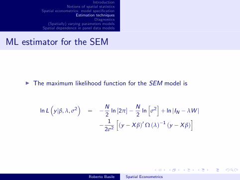
IntroductionNotions of spatial statistics
Spatial econometrics: model specificationEstimation techniques
Diagnostics(Spatially) varying parameters models
Spatial dependence in panel data models
ML estimator for the SEM
I The maximum likelihood function for the SEM model is
lnL(y |β,λ, σ2
)= −N
2ln [2π]− N
2ln[σ2]+ ln |IN − λW |
− 1
2σ2
[(y −X β)′Ω (λ)−1 (y −X β)
]
Roberto Basile Spatial Econometrics

IntroductionNotions of spatial statistics
Spatial econometrics: model specificationEstimation techniques
Diagnostics(Spatially) varying parameters models
Spatial dependence in panel data models
ML estimator for the SEM
I The GLS results for β and Var (β) are also ML. Thus, we can usethem to compute the concentrated log-likelihood as a nonlinearfunction of the autoregressive parameter λ
lnL (y |λ) = −N
2ln [2π] +
N
∑i=1
(IN − λωi )
−N
2ln[e ′GLS (IN − λW )′ (IN − λW ) eGLS
]eGLS = y −X βGLS
Roberto Basile Spatial Econometrics

IntroductionNotions of spatial statistics
Spatial econometrics: model specificationEstimation techniques
Diagnostics(Spatially) varying parameters models
Spatial dependence in panel data models
Iterative approach to estimate the SEM
I 1) Estimate y = X β + ε by OLS and calculate associated residuals
β(1) =(X ′X
)−1X ′y u(1) = y − X β(1)
I 2) Use these residuals to find a value of λ that maximizes thelog-likelihood conditional on the βOLS values
lnL (y |λ) = −N
2ln [2π]− N
2ln[u′ (IN − λW )′ (IN − λW ) u
]+∑
i
(IN − λωi )
I 3) Updates the values of β using the value of λ determined in step2):
βFGLS =
[X ′(IN − λW
)′ (IN − λW
)X
]−1
X ′(IN − λW
)′ (IN − λW
)y
Roberto Basile Spatial Econometrics

IntroductionNotions of spatial statistics
Spatial econometrics: model specificationEstimation techniques
Diagnostics(Spatially) varying parameters models
Spatial dependence in panel data models
Iterative approach to estimating the SEM
I This approach is continued until convergence is achieved and weobtain:
β(step k) ≈ β(step k−1) and λ(step k) ≈ λ(step k−1)
Roberto Basile Spatial Econometrics

IntroductionNotions of spatial statistics
Spatial econometrics: model specificationEstimation techniques
Diagnostics(Spatially) varying parameters models
Spatial dependence in panel data models
Nonparametric covariance matrix estimator
I Kelejian, H.H. and Prucha, I.R. (2007) HAC estimation in a spatialframework, Journal of Econometrics, 140, pages 131–154
I The basic idea is to avoid specifying a particular spatial process of aparticular spatial weights matrix and to extract the spatialcovariance terms from weighted averages of cross-products ofresiduals, using a kernel function
I This yields the so-called heteroskedastic and spatial autocorrelation(HAC) estimator (similar to Newey-West approach)
I A major practical problem is to ensure that the estimatedvaiance-covariance matrix is positive definite
Roberto Basile Spatial Econometrics

IntroductionNotions of spatial statistics
Spatial econometrics: model specificationEstimation techniques
Diagnostics(Spatially) varying parameters models
Spatial dependence in panel data models
IV-2SLS estimator for the SLM
I The endogeneity of the spatially lagged dependent variable can alsobe addressed by means of an instrumental variables or 2SLSapproach (Anselin, 1988; Kelejian and Robinson, 1993; Kelejian andPrucha, 1998)
I Structural modely = ρWy + X β + ε
I Rewrite the model compactly
y = Qδ + ε
where Q = (Wy , X ) and δ = (β, ρ)
Roberto Basile Spatial Econometrics

IntroductionNotions of spatial statistics
Spatial econometrics: model specificationEstimation techniques
Diagnostics(Spatially) varying parameters models
Spatial dependence in panel data models
IV-2SLS estimator for the SLM
I 2SLS estimation of the model using the instruments Z
Wy = δZ + η
δ =(Z ′Z
)−1Z ′Wy
Wy = HWy H = Z(Z ′Z
)−1Z ′
Q =(X , Wy
)y = Qδ + ε
δ =(Q ′Q
)−1Q ′y
Roberto Basile Spatial Econometrics

IntroductionNotions of spatial statistics
Spatial econometrics: model specificationEstimation techniques
Diagnostics(Spatially) varying parameters models
Spatial dependence in panel data models
IV-2SLS estimator for the SLM
I As demonstrated in Kelejian and Robinson (1993), the choice of aninstrument for Wy follows from conditional expectation in thereduced form
E [y |X ] = (IN − ρW )−1 X β
= X β + ρWX β + ρ2W 2X β + ...
I Apart from the exogenous variables X (which are alwaysinstruments), this includes their spatial lags as well, suggesting WXas a set of instruments
Roberto Basile Spatial Econometrics

IntroductionNotions of spatial statistics
Spatial econometrics: model specificationEstimation techniques
Diagnostics(Spatially) varying parameters models
Spatial dependence in panel data models
A generalized 2SLS procedure for SARSAR
Kelejian and Prucha (1998)
I Structural form
y = ρWy + X β + ε
ε = λW ε + u
I Variance-covariance matrix:
Ωε = E(εε′)= σ2
u (IN − λW )−1 (IN − λW )−1
I Let Z =(X , WX , W 2X , ...
)the matrix of instruments
I Rewrite the model more compactly
y = Qδ + ε ε = λW ε + u
where Q = (Wy , X ) and δ = (β, ρ)
Roberto Basile Spatial Econometrics

IntroductionNotions of spatial statistics
Spatial econometrics: model specificationEstimation techniques
Diagnostics(Spatially) varying parameters models
Spatial dependence in panel data models
Three step procedure
I First step: 2SLS estimation of the model using the instruments ZI Second step: GM estimation of λ using the residuals from the first
step (based on three moment conditions on u )I Third step
I Application of the Cochrane-Orcutt type transformation:
y∗ = Q∗δ + u
y∗ = y − λWy
Q∗ = Q − λWZ
I Re-estimation of the regression model after theCochrane-Orcutt transformation to account for the spatialcorrelation in the residualsδ =
(Q(
λ)′
Q(
λ))−1
Q(
λ)′
y(
λ)
Roberto Basile Spatial Econometrics

IntroductionNotions of spatial statistics
Spatial econometrics: model specificationEstimation techniques
Diagnostics(Spatially) varying parameters models
Spatial dependence in panel data models
A list of references for 2SLS and GMM approaches to SLM
I Das, D., Kelejian, H.H., Prucha, I.R., 2003. Small sample propertiesof estimators of spatial autoregressive models with autoregressivedisturbances. Papers in Regional Science 82, 1–26
I Kelejian, H.H., Prucha, I.R., 1997. Estimation of spatial regressionmodels with autoregressive errors by two-stage least squaresprocedures: a serious problem. International Regional ScienceReview 20, 103–111
I Kelejian, H.H., Prucha, I.R., 1998. A generalized spatial two-stageleast squares procedure for estimating a spatial autoregressive modelwith autoregressive disturbances. Journal of Real Estate Financeand Economics 17, 99–121
Roberto Basile Spatial Econometrics

IntroductionNotions of spatial statistics
Spatial econometrics: model specificationEstimation techniques
Diagnostics(Spatially) varying parameters models
Spatial dependence in panel data models
A list of references for 2SLS and GMM approaches to SLM
I Kelejian, H.H., Prucha, I.R., 1999. A generalized momentsestimator for the autoregressive parameter in a spatial model.International Economic Review 40, 509–533
I Kelejian, H.H., Prucha, I.R., Yuzefovich, E., 2004, Instrumentalvariable estimation of a spatial autorgressive model withautoregressive disturbances: large and small sample results. In:LeSage, J., Pace, R.K. (Eds.), Spatial and SpatiotemporalEconometrics, Advances in Econometrics, Vol. 18. Elsevier, NewYork, pp. 163–198
I Lee, L.F., 2001a. Generalized method of moments estimation ofspatial autoregressive processes. Mimeo, Department of Economics,Ohio State University
Roberto Basile Spatial Econometrics

IntroductionNotions of spatial statistics
Spatial econometrics: model specificationEstimation techniques
Diagnostics(Spatially) varying parameters models
Spatial dependence in panel data models
A list of references for 2SLS and GMM approaches to SLM
I Lee, L.F., 2001b. GMM and 2SLS estimation of mixed regressive,spatial autoregressive models. Mimeo, Department of Economics,Ohio State University
I Lee, L.F., 2002. Consistency and efficiency of least squaresestimation for mixed regressive, spatial autoregressive models.Econometric Theory 18, 252–277
I Lee, L.F., 2003. Best spatial two-stage least squares estimators fora spatial autoregressive model with autoregressive disturbances.Econometric Reviews 22, 307–335
Roberto Basile Spatial Econometrics

IntroductionNotions of spatial statistics
Spatial econometrics: model specificationEstimation techniques
Diagnostics(Spatially) varying parameters models
Spatial dependence in panel data models
Course content
I Introduction
I Notions of spatial statistics
I Spatial econometrics: model specification
I Estimation techniques
I Diagnostics
I (Spatially) varying parameters models
I Spatial dependence in panel data models
Roberto Basile Spatial Econometrics

IntroductionNotions of spatial statistics
Spatial econometrics: model specificationEstimation techniques
Diagnostics(Spatially) varying parameters models
Spatial dependence in panel data models
Moran’s I test of spatial autocorrelation in OLS residuals
I With W standardized
I =e ′We
e ′e
where e is a vector of OLS residuals
I Interpretation not straightforward: while the null hypothesis isobviously the absence of spatial dependence, a precise expression forthe alternative hypothesis does not exit
I Cliff and Ord (1972, 1973, 1981) show that the asymptoticdistribution for Moran’s I based on least-squares residualscorresponds to a standard normal distribution after havingstandardized the I-statistic
Roberto Basile Spatial Econometrics

IntroductionNotions of spatial statistics
Spatial econometrics: model specificationEstimation techniques
Diagnostics(Spatially) varying parameters models
Spatial dependence in panel data models
Moran’s I test of spatial autocorrelation in OLS residuals
I W standardized
E [I ] = tr (MW ) / (N − k)
V [I ] =tr (MWMW ′) + tr (MW )2 + [tr (MW )]2
(N − k) (N − k − 2)− E [I ]2
z [I ] =I − E (I )√
V [I ]
I Under H0, za∼ N (0, 1)
Roberto Basile Spatial Econometrics

IntroductionNotions of spatial statistics
Spatial econometrics: model specificationEstimation techniques
Diagnostics(Spatially) varying parameters models
Spatial dependence in panel data models
Likelihood-based tests
ML Tests against spatial error
I Classical tests based on log-likelihood, its first derivative (score)and its second derivative (information matrix)
I Wald (W )I Likelihood ratio (LR)I Lagrange multiplier (LM)
I RequirementsI W : alternative (SEM model)I LR : both null and alternativeI LM : null (OLS residuals) (most conservative)
I Asymptotic result : W=LR=LM
I Finite sample inequality : W>LR>LM
Roberto Basile Spatial Econometrics

IntroductionNotions of spatial statistics
Spatial econometrics: model specificationEstimation techniques
Diagnostics(Spatially) varying parameters models
Spatial dependence in panel data models
Likelihood-based tests
I Consider the simple null hypothesis H0 : θ = θ0
Roberto Basile Spatial Econometrics

IntroductionNotions of spatial statistics
Spatial econometrics: model specificationEstimation techniques
Diagnostics(Spatially) varying parameters models
Spatial dependence in panel data models
Likelihood ratio test
I Define
λ =max L (θ) under the restrictions
max L (θ) without the restrictions< 1
I Consider the simple null hypothesis for a scalar parameterH0 : θ = θ0
I If H0 : θ = θ0 is not valid, λ will be significantly ¡ 1
I If H0 : θ = θ0 is valid, λ will be close to 1
I The LR statistic is defined as
LR = −2 ln λ
I Under H0, LRa∼ χ2
1
Roberto Basile Spatial Econometrics

IntroductionNotions of spatial statistics
Spatial econometrics: model specificationEstimation techniques
Diagnostics(Spatially) varying parameters models
Spatial dependence in panel data models
Wald test
I In the simple case H0 : θ = θ0 , the Wald test verifies whether the
difference(
θ − θ0
)is significant. If H0 : θ = 0
W =θ2
V[(
θ)] = z2
I Under H0, Wa∼ χ2
1
Roberto Basile Spatial Econometrics

IntroductionNotions of spatial statistics
Spatial econometrics: model specificationEstimation techniques
Diagnostics(Spatially) varying parameters models
Spatial dependence in panel data models
Lagrange Multiplier test
I The LM test uses a statistic based on the score, S (θ) , of theunrestricted ML function evaluated in correspondence of θ0 . If therestriction is valid, then the restricted estimator should be near thepoint that maximizes the log-likelihood. That is, the slope of thelog-likelihood function should be near zero at the restrictedestimator: S (θ0) = 0
I In other words the LM test verifies whether the value of S (θ0) issignificantly different from zero
LM = N−1S ′ (θ0) I (θ0)−1 S ′ (θ0)
I Under H0 , LMa∼ χ2
1
Roberto Basile Spatial Econometrics

IntroductionNotions of spatial statistics
Spatial econometrics: model specificationEstimation techniques
Diagnostics(Spatially) varying parameters models
Spatial dependence in panel data models
LM-error
I Only requires estimation of the model under the null
I H0 : no spatial autocorrelation (λ = 0)
I H1 : spatial error model (λ 6= 0)
LMerr =[
e ′We/σ2]2
/T
where e denotes least-squares residuals andT = tr (WW ) + (W ′W )
I LMerr and the square of Moran’s I are asymptotically equivalent
I Under H0 , LMa∼ χ2
1
Roberto Basile Spatial Econometrics

IntroductionNotions of spatial statistics
Spatial econometrics: model specificationEstimation techniques
Diagnostics(Spatially) varying parameters models
Spatial dependence in panel data models
Wald and Likelihood ratio tests (SEM vs OLS)
I Wald test: Asymptotic t-test on λ in SEM. Requires only MLestimates and asymptotic variance
I LR test: requires both OLS and ML of SEM model
LR = N[
ln σ2OLS − ln σ2
SEM
]+ 2Σi ln (1− λωi )
with ωi as the eigenvalues of W
I Under H0, W and LRa∼ χ2
1
Roberto Basile Spatial Econometrics

IntroductionNotions of spatial statistics
Spatial econometrics: model specificationEstimation techniques
Diagnostics(Spatially) varying parameters models
Spatial dependence in panel data models
LM-lag test statistic
I Only requires estimation of the model under the null
I H0 : no spatial autocorrelation (ρ = 0)
I H1 : spatial lag model (ρ 6= 0)
LMlag =[
e ′Wy/σ2]2
/R
R =(
WX β)′
M(
WX β)
/σ2OLS + tr
(WW + W ′W
)I No connection with Moran’s I
I Under H0, LMa∼ χ2
1
Roberto Basile Spatial Econometrics

IntroductionNotions of spatial statistics
Spatial econometrics: model specificationEstimation techniques
Diagnostics(Spatially) varying parameters models
Spatial dependence in panel data models
Wald and likelihood ratio tests (SLM vs OLS)
I Wald test: Asymptotic t-test on ρ in SLM. Requires only MLestimates
I LR test: requires both OLS and ML of spatial lag model
LR = N[
ln σ2OLS − ln σ2
SLM
]+ 2Σi ln (1− λωi )
I Under H0, LRa∼ χ2
1
Roberto Basile Spatial Econometrics

IntroductionNotions of spatial statistics
Spatial econometrics: model specificationEstimation techniques
Diagnostics(Spatially) varying parameters models
Spatial dependence in panel data models
Specification-robust LM tests
I Local misspecification
I LMerr and LM lag are no longer χ21 under H0 in the
presence of local misspecification in the form of the other typeof spatial dependence
I In the presence of spatial lag dependence, the LMerr testagainst error correlation becomes biased, and, in the presenceof spatial error dependence the LM lag test against spatial lagbecomes biased
I LM tests will tend to reject H0 too oftenI Robust to local misspecification (Anselin and Bera, 1992)
Roberto Basile Spatial Econometrics

IntroductionNotions of spatial statistics
Spatial econometrics: model specificationEstimation techniques
Diagnostics(Spatially) varying parameters models
Spatial dependence in panel data models
Specification-robust LM tests
I Test for spatial error robust to spatial lag: RLMerr
LM∗λ =[dλ −Tσ2C−1dρ
]2 /[T(1−Tσ2C
)]I Test for spatial lag robust to spatial error: RLM lag
LM∗ρ =[dρ − dλ
]2 /[C/σ2 −T
]C =
(WX β
)′M(WX β
)+Tσ2
dλ = −tr (IN − λW )−1 W + e′We/σ2 score of the ML of the SEM
dρ = −tr (IN − ρW )−1 W + e′We/σ2 score of the ML of the SLM
I InterpretationI LMerr and LM lag are often both highly significantI Typically, only one of the robust test will be significantI Significant one (or most significant one) points to proper
spatial alternative (error or lag)Roberto Basile Spatial Econometrics

IntroductionNotions of spatial statistics
Spatial econometrics: model specificationEstimation techniques
Diagnostics(Spatially) varying parameters models
Spatial dependence in panel data models
Specification search
I Types of specification search
I A) Forward step-wise strategy
I start from constrained models (OLS)I base model selection on diagnostics
I B) Backward step-wise strategy
I start from unconstrained modelI higher-order spatial modelI test constraints and proceed to simpler modelsI common factor constraint
Roberto Basile Spatial Econometrics

IntroductionNotions of spatial statistics
Spatial econometrics: model specificationEstimation techniques
Diagnostics(Spatially) varying parameters models
Spatial dependence in panel data models
Specification search - Forward
I OLS estimation - LM tests
I None significant
I Stay with OLS results
I LM-error significant, LM-lag not significant
I Error model
I LM-lag significant, LM-error not significant
I lag model
I both LM-error and LM-lag significant
I go with robust tests and select one with highestsignificance as alternative
Roberto Basile Spatial Econometrics

IntroductionNotions of spatial statistics
Spatial econometrics: model specificationEstimation techniques
Diagnostics(Spatially) varying parameters models
Spatial dependence in panel data models
Practical considerations
I Choice of weights important
I Spatial dependence and heteroskedasticity related
I Importance of distinguishing between lag and error
I These are large sample tests
Roberto Basile Spatial Econometrics

IntroductionNotions of spatial statistics
Spatial econometrics: model specificationEstimation techniques
Diagnostics(Spatially) varying parameters models
Spatial dependence in panel data models
LM error test in spatial lag model
I Based on ML-lag residuals
I Use full likelihood, constrain λ = 0 in score and information matrix
LMλ|ρ =(e ′We/σ2
)2[T − TAvar (ρ)]−1
T = tr(WW + W ′W
)TA = tr
[(WW + W ′W
)(I − ρW )−1
]
Roberto Basile Spatial Econometrics

IntroductionNotions of spatial statistics
Spatial econometrics: model specificationEstimation techniques
Diagnostics(Spatially) varying parameters models
Spatial dependence in panel data models
LM lag test in spatial error model
I Based on ML-error residuals
I Use full likelihood, constrain ρ = 0 in score and information matrix
I Define
I B = (IN − λW ) and e = ML residualsI Hp =
tr (WW ) + tr[BWB−1′] [BWB−1
]+ [BWXb]′ [BWXb] /σ2
I Hλρ =[(BX )′ BWX β/σ2, tr
(WB−1
)BWB−1 + trWWB−1, 0
]LMρ|λ =
[e ′B
′BWy
]2 [Hp −Hλρvar (λ)H
′λρ
]−1
Roberto Basile Spatial Econometrics

IntroductionNotions of spatial statistics
Spatial econometrics: model specificationEstimation techniques
Diagnostics(Spatially) varying parameters models
Spatial dependence in panel data models
Example: Regional Economic Growth in Europe
Mankiw et al. (1992)
γy = β ln y0 + ψX + ε
γy : Productivity growth rateln y0 : initial labour productivityX : vector of structural variables (includes also a constant term)ε : vector of iidN errors
Roberto Basile Spatial Econometrics

IntroductionNotions of spatial statistics
Spatial econometrics: model specificationEstimation techniques
Diagnostics(Spatially) varying parameters models
Spatial dependence in panel data models
Example: Regional Economic Growth in Europe
I Ertur and Koch (2007) propose a modified version of the MRWgrowth model (SDM)
γy = β ln y0 + χW ln y0 + ψX + θWX + ρW γy + ε
Reduced form:
γy = (IN − ρW )−1 ln y0β + (IN − ρW )−1 W ln y0χ
+ (IN − ρW )−1 X ψ + (IN − ρW )−1 WX θ + (IN − ρW )−1 ε
I Thus, the outcome in a location i is influenced not only by theexogenous characteristics of i, but also by those in all other locationsthrough the inverse spatial transformation (IN − ρW )−1 . A spatialdiffusion process of random shocks appears also in this case
Roberto Basile Spatial Econometrics

IntroductionNotions of spatial statistics
Spatial econometrics: model specificationEstimation techniques
Diagnostics(Spatially) varying parameters models
Spatial dependence in panel data models
Example: Regional Economic Growth in Europe
I The SEM is specified as:
γy = β ln y0 + ψX + ε
ε = ϕW ε + v v ∼ iidN(
o, σ2v IN
)Reduced form:
γy = β ln y0 + ψX + θWX + (IN − ϕW )−1 v
I Only random shocks diffuse across economies, while there are nosubstantive spatial externalities. However, the reduced form of theSEM can also be written as:
γy = β ln y0 − ϕβW ln y0 + ψX − ϕψWX + ϕW γy + v
Roberto Basile Spatial Econometrics

IntroductionNotions of spatial statistics
Spatial econometrics: model specificationEstimation techniques
Diagnostics(Spatially) varying parameters models
Spatial dependence in panel data models
Example: Regional Economic Growth in Europe
I This represents a constrained version of the SDM, whose reducedform implies the existence of substantive spatial externalities. Therestriction can be assessed through the common factor test
Roberto Basile Spatial Econometrics

IntroductionNotions of spatial statistics
Spatial econometrics: model specificationEstimation techniques
Diagnostics(Spatially) varying parameters models
Spatial dependence in panel data models
Using R functions: Linear estimation of a regional growthregression Solow model
LinearSolow < − lm(gprb v log(pr80b) + lninv1b + lnagrib +lndens emp,data=EUselected1)summary(LinearSolow)
Estimate Std.Error t value Pr( > |t|)(Intercept) -0.0016380 0.0024756 -0.662 0.50901log(pr80b) -0.0118647 0.0009465 -12.535 < 2e-16 ***lninv1b 0.0007924 0.0003034 2.612 0.00974 **lnagrib -0.0010129 0.0003701 -2.737 0.00680**lndens emp 0.0006336 0.0004341 1.459 0.14613
Residual standard error: 0.004737 on 185 degrees of freedom MultipleR-squared: 0.498, Adjusted R-squared: 0.4872 F-statistic: 45.89 on 4and 185 DF, p-value: < 2.2e-16
Roberto Basile Spatial Econometrics

IntroductionNotions of spatial statistics
Spatial econometrics: model specificationEstimation techniques
Diagnostics(Spatially) varying parameters models
Spatial dependence in panel data models
Using R functions: Test spatial dependence for OLSresiduals
# Moran’s I test for OLS residuals using different spatial weights matriceslm.morantest(LinearSolow,dnb320.listw,resfun=rstudent)...lm.morantest(LinearSolow,dnb720.listw,resfun=rstudent)
Roberto Basile Spatial Econometrics

IntroductionNotions of spatial statistics
Spatial econometrics: model specificationEstimation techniques
Diagnostics(Spatially) varying parameters models
Spatial dependence in panel data models
Using R functions: Global Moran’s I for regression residuals
> lm.morantest(LinearSolow,dnb720.listw,resfun=rstudent)data:model: lm(formula = gprb v log(pr80b) + lninv1b + lnagrib +lndens emp, data = EUselected1)weights: dnb720.listwMoran I statistic standard deviate = 5.7305, p-value = 5.006e-09alternative hypothesis: greatersample estimates:Observed Moran’s I Expectation Variance0.0680336306 -0.0090199633 0.0001807995
Roberto Basile Spatial Econometrics

IntroductionNotions of spatial statistics
Spatial econometrics: model specificationEstimation techniques
Diagnostics(Spatially) varying parameters models
Spatial dependence in panel data models
Using R functions: Lagrange multiplier spatial dependencetest for OLS residuals
I res < − lm.LMtests(LinearSolow, dnb420.listw,test=”all”)I tres < − t(sapply(res, function(x) c(x$statistic, x$parameter,
x$p.value)))I colnames(tres) < − c(”Statistic”, ”df”, ”p-value”)I printCoefmat(tres)
Statistic df p-valueLMerr 15.43620 1.00000 0.0001LMlag 4.22923 1.00000 0.0397RLMerr 12.16501 1.00000 0.0005RLMlag 0.95803 1.00000 0.3277SARMA 16.39423 2.00000 0.0003
Roberto Basile Spatial Econometrics

IntroductionNotions of spatial statistics
Spatial econometrics: model specificationEstimation techniques
Diagnostics(Spatially) varying parameters models
Spatial dependence in panel data models
Using R functions: Spatial Durbin model (ML estimates)
The choice of the spatial weight matrix to estimate the SDM: modeluncertaintyBase the choice on the value of the AIC
SDM320 < − lagsarlm(formula(LinearSolow),listw=dnb320.listw,type=”mixed”,method=”eigen”,data=EUselected1)
...
SDM1020 < − lagsarlm(formula(LinearSolow),listw=dnb1020.listw,type=”mixed”,method=”eigen”,data=EUselected1)
Roberto Basile Spatial Econometrics

IntroductionNotions of spatial statistics
Spatial econometrics: model specificationEstimation techniques
Diagnostics(Spatially) varying parameters models
Spatial dependence in panel data models
Using R functions
summary(SDM420, correlation=F)
Estimate Std. Error z value Pr(> |z|)(Intercept) -2.770 78.2676 -0.0354 0.9717645log(pr80b) -159.016 18.5123 -8.5898 < 2.2e-16lninv1b 1.973 3.1674 0.6232 0.5331778lnagrib -12.413 3.7957 -3.2703 0.0010742lndens emp 9.981 4.3459 2.2968 0.0216307lag.log(pr80b) 95.960 27.8844 3.4414 0.0005788lag.lninv1b 18.669 9.7521 1.9144 0.0555658lag.lnagrib 1.3004 9.5782 0.1358 0.8920039lag.lndens emp -2.6614 11.9504 -0.2227 0.8237680
Roberto Basile Spatial Econometrics

IntroductionNotions of spatial statistics
Spatial econometrics: model specificationEstimation techniques
Diagnostics(Spatially) varying parameters models
Spatial dependence in panel data models
Using R functions
Rho: 0.36116, LR test value: 5.2777, p-value: 0.0216Asymptotic standard error: 0.14576 z-value: 2.4777, p-value:0.013222Wald statistic: 6.1392, p-value: 0.013222Log likelihood: -989.6833 for mixed modelML residual variance (sigma squared): 1938.6, (sigma: 44.03)LM test for residual autocorrelation test value: 0.00069044, p-value:0.97904
Roberto Basile Spatial Econometrics

IntroductionNotions of spatial statistics
Spatial econometrics: model specificationEstimation techniques
Diagnostics(Spatially) varying parameters models
Spatial dependence in panel data models
Using R functions: Compute average direct and indirecteffects
W < − as(as dgRMatrix listw(dnb420.listw),”CsparseMatrix”)trMatc < − trW(W, type=”mult”)trMC < − trW(W, type=”MC”)SDM420.impact < − impacts(SDM420, tr=trMatc,R=200)summary(SDM420.impact, zstats=TRUE, short=TRUE)
Estimate Direct Indirect Totallog(pr80b) -1.590 -1.578 0.591 -0.987lninv1b 0.020 0.026 0.297 0.323lnagrib -0.124 -0.125 -0.049 -0.174lndens emp 0.100 0.100 0.014 0.115
Roberto Basile Spatial Econometrics

IntroductionNotions of spatial statistics
Spatial econometrics: model specificationEstimation techniques
Diagnostics(Spatially) varying parameters models
Spatial dependence in panel data models
Using R functions: Spatial lag model (Maximum likelihoodestimates
SAR420 < − lagsarlm(formula(LinearSolow), listw=dnb420.listw,type=”lag”, method=”eigen”,data=EUselected1)summary(SAR420, correlation=F)
Estimate Std.Error z value Pr(< |z|)(Intercept) -14.317 24.212 -0.591 0.554log(pr80b) -103.731 14.662 -7.074 1.498e-12lninv1b 7.535 2.972 2.534 0.011lnagrib -9.543 3.633 -2.627 0.008lndens emp 6.245 4.246 1.470 0.141
Roberto Basile Spatial Econometrics

IntroductionNotions of spatial statistics
Spatial econometrics: model specificationEstimation techniques
Diagnostics(Spatially) varying parameters models
Spatial dependence in panel data models
Using R functions: Spatial lag model (Maximum likelihoodestimates
Rho: 0.19951, LR test value: 3.1106, p-value: 0.077785Asymptotic standard error: 0.12323z-value: 1.619, p-value: 0.10544
Wald statistic: 2.6213, p-value: 0.10544Log likelihood: -998.527 for lag modelML residual variance (sigma squared): 2143.2, (sigma: 46.295)AIC: 2011.1, (AIC for lm: 2012.2)LM test for residual autocorrelation test value: 6.7246, p-value:0.0095091
Roberto Basile Spatial Econometrics

IntroductionNotions of spatial statistics
Spatial econometrics: model specificationEstimation techniques
Diagnostics(Spatially) varying parameters models
Spatial dependence in panel data models
Using R functions: Compare SDM and SAR
LR.sarlm(SDM420,SAR420)
Likelihood ratio = 17.6873, df = 4, p-value = 0.00142
Roberto Basile Spatial Econometrics

IntroductionNotions of spatial statistics
Spatial econometrics: model specificationEstimation techniques
Diagnostics(Spatially) varying parameters models
Spatial dependence in panel data models
Using R functions: Spatial Error model (ML estimates)
error420 < − errorsarlm(formula=formula(LinearSolow),listw=dnb420.listw,method=”eigen”,data=EUselected1)summary(error420)
Estimate Std.Error z value Pr(> |z|)(Intercept) -12.685 23.8353 -0.5322 0.594591log(pr80b) -136.840 13.6350 -10.0360 ¡ 2.2e-16lninv1b 4.066 3.0909 1.3156 0.188311lnagrib -10.787 3.7492 -2.8773 0.004011lndens emp 8.4469 4.2607 1.9825 0.047421
Roberto Basile Spatial Econometrics

IntroductionNotions of spatial statistics
Spatial econometrics: model specificationEstimation techniques
Diagnostics(Spatially) varying parameters models
Spatial dependence in panel data models
Using R functions: Spatial Error model (ML estimates)
Lambda: 0.52865, LR test value: 12.024, p-value: 0.00052526Asymptotic standard error: 0.12109z-value: 4.3659, p-value: 1.2662e-05
Wald statistic: 19.061, p-value: 1.2662e-05Log likelihood: -994.0704 for error modelML residual variance (sigma squared): 2002.2, (sigma: 44.746)AIC: 2002.1, (AIC for lm: 2012.2)
Roberto Basile Spatial Econometrics

IntroductionNotions of spatial statistics
Spatial econometrics: model specificationEstimation techniques
Diagnostics(Spatially) varying parameters models
Spatial dependence in panel data models
Using R functions: Common factor test
LR.sarlm(SDM420,error420)
Likelihood ratio = 8.7741, df = 4, p-value = 0.067
Roberto Basile Spatial Econometrics

IntroductionNotions of spatial statistics
Spatial econometrics: model specificationEstimation techniques
Diagnostics(Spatially) varying parameters models
Spatial dependence in panel data models
Course content
I Introduction
I Notions of spatial statistics
I Spatial econometrics: model specification
I Estimation techniques
I Diagnostics
I (Spatially) varying parameters models
I Spatial dependence in panel data models
Roberto Basile Spatial Econometrics

IntroductionNotions of spatial statistics
Spatial econometrics: model specificationEstimation techniques
Diagnostics(Spatially) varying parameters models
Spatial dependence in panel data models
(Spatially) varying parameters models
I The spatial expansion method (trend surface): Casetti (1972, 1997)
I Geographically weighted regression: Fotheringham, Brunsdon, andCharlton (2002)
I Spatial econometric STAR Models: Pede, Florax, Lambert and Holt(2010)
I Semiparametric spatial additive models: Gress (2004), Basile andGress (2004), Basile (2008, 2009)
Roberto Basile Spatial Econometrics

IntroductionNotions of spatial statistics
Spatial econometrics: model specificationEstimation techniques
Diagnostics(Spatially) varying parameters models
Spatial dependence in panel data models
Spatial expansion (trend surface)
I Global model:
yi=α + βx1i+... + τxmi+εi i is a point in space or a region
I It can be expanded by allowing each of the parameters to be afunction of spatial coordinates
αi = α0 + α1ni + α2ei
βi = β0 + β1ni + β2ei
...
τi = τ0 + τ1ni + τ2ei
where ni (northing) and ei (easting) are the spatial coordinates oflocation i
yi=α0 + α1ni + α2ei + β0x1i + β1nix1i + β2eix1i + ... + τ0xmi + τ1nixmi + τ2eixmi + εi
Roberto Basile Spatial Econometrics

IntroductionNotions of spatial statistics
Spatial econometrics: model specificationEstimation techniques
Diagnostics(Spatially) varying parameters models
Spatial dependence in panel data models
Spatial expansion (trend surface)
I This model can be estimated by OLS or ML (if the model is aPoisson or a logit regression or if it contains spatial autoregressiveparameters) to get spatial varying parameter estimates
I Marginal effects:∂y
∂x1= β0 + β1n + β2e
Roberto Basile Spatial Econometrics

IntroductionNotions of spatial statistics
Spatial econometrics: model specificationEstimation techniques
Diagnostics(Spatially) varying parameters models
Spatial dependence in panel data models
Limitations of the spatial expansion method
I It displays trend in relationships over space, while obscuringimportant local variations
I The form of the expansion equations needs to be assumed a priori
I The expansion equations must be deterministic to remove problemsof estimation in the terminal model
I All three problems can be overcome in GWR
Roberto Basile Spatial Econometrics

IntroductionNotions of spatial statistics
Spatial econometrics: model specificationEstimation techniques
Diagnostics(Spatially) varying parameters models
Spatial dependence in panel data models
Geographically Weighted Regression
I Fotheringham, A.S., Brunsdon, C., and Charlton, M.E., 2002,Geographically Weighted Regression, Chichester: Wiley;http://www.nuim.ie/ncg/GWR/index.htm
Roberto Basile Spatial Econometrics

IntroductionNotions of spatial statistics
Spatial econometrics: model specificationEstimation techniques
Diagnostics(Spatially) varying parameters models
Spatial dependence in panel data models
GWR
I Global model
yi = a0 + ∑k
αkxik + εi i : a point in space or a region
I OLS estimation:
α =(X ′X
)−1X ′y
I GWR extends the traditional regression framework by allowing localrather than global parameters to be estimated
yi = α0 (ni , ei ) + ∑k
αk (ni , ei ) xik + εi
where (ni , ei ) denotes the coordinates of the i -th point in space,αk (ni , ei ) is a realization of the continuous function αk (n, e) atpoint i
Roberto Basile Spatial Econometrics

IntroductionNotions of spatial statistics
Spatial econometrics: model specificationEstimation techniques
Diagnostics(Spatially) varying parameters models
Spatial dependence in panel data models
GWR
I In the estimation of the GWR model it is assumed that observeddata near to point i have more of an influence in the estimation ofthe αk (n, e) than do data located farther from i . In essence, theequation measures the relationships inherent in the model aroundeach point i
I For a given data set, local parameters αk (n, e) are estimated usingthe WLS procedure. The weights wij for j = 1, ...,N, at eachlocation (ni , ei ) are obtained as a continuous kernel function of thedistance between the point i and the other data points
Roberto Basile Spatial Econometrics

IntroductionNotions of spatial statistics
Spatial econometrics: model specificationEstimation techniques
Diagnostics(Spatially) varying parameters models
Spatial dependence in panel data models
GWR
I Let
α =
α0 (n1, e1) α1 (n1, e1) · · · αK (n1, e1)...
.... . .
...α0 (nn, en) α1 (nn, en) · · · αK (nn, en)
be the matrix of the local parameters. Each row is estimated by
α (i) =(
XTW (i)X)−1
XTW (i) y
where
W (i) = diag [wi1, wi2, ..., win]
Roberto Basile Spatial Econometrics

IntroductionNotions of spatial statistics
Spatial econometrics: model specificationEstimation techniques
Diagnostics(Spatially) varying parameters models
Spatial dependence in panel data models
GWR
I Several different weighting functions can be defined, the morecommon kernels being the Gaussian and the bi-square weightingfunctions
I Gaussian weights
wij = exp(−d2
ij/h2)
I A modified bi-square function taking into account only the Nnearest neighbours is
wij =[
1−(dij/hi
)2]2
if dij < hi
wij = 0 otherwise
where hi is the Nth nearest-neighbour distance from i
Roberto Basile Spatial Econometrics

IntroductionNotions of spatial statistics
Spatial econometrics: model specificationEstimation techniques
Diagnostics(Spatially) varying parameters models
Spatial dependence in panel data models
GWR
I This kernel function varies in space and presents an adaptivebandwidth depending on the data points density. Consequently, thecalibration of the model involves also the choice of N , the numberof data point to be included in the estimation of local parameters
Roberto Basile Spatial Econometrics

IntroductionNotions of spatial statistics
Spatial econometrics: model specificationEstimation techniques
Diagnostics(Spatially) varying parameters models
Spatial dependence in panel data models
GWR
Roberto Basile Spatial Econometrics

IntroductionNotions of spatial statistics
Spatial econometrics: model specificationEstimation techniques
Diagnostics(Spatially) varying parameters models
Spatial dependence in panel data models
GWR
Roberto Basile Spatial Econometrics

IntroductionNotions of spatial statistics
Spatial econometrics: model specificationEstimation techniques
Diagnostics(Spatially) varying parameters models
Spatial dependence in panel data models
GWR
I The appropriate bandwidth, or the appropriate value of N , can beobtained by a least square approach using the cross-validationcriteria
CV =n
∑i=1
[yi − y 6=i (hi )
]2where y 6=i (hi ) is the fitted value of yi with the observations for
point i omitted from the calibration process
Roberto Basile Spatial Econometrics

IntroductionNotions of spatial statistics
Spatial econometrics: model specificationEstimation techniques
Diagnostics(Spatially) varying parameters models
Spatial dependence in panel data models
A critical point
I There are parallels between GWR and kernel regression. Inkernel regression, y is modelled as a non-linear function of Xby weighting data in attribute space rather than geographicalspace
I Only when the two criteria (weighting data in attribute spaceand in geographical space) match, we have similar results
I With GWR we miss important non-linearities if the data arenot spatially clustered
Roberto Basile Spatial Econometrics

IntroductionNotions of spatial statistics
Spatial econometrics: model specificationEstimation techniques
Diagnostics(Spatially) varying parameters models
Spatial dependence in panel data models
Spatial econometric STAR Models: Pede et al. (2010)
I Pede et al. (2010) investigate nonlinearity in spatial processmodels allowing for gradual regime-switching structures in theform of a smooth transition autoregressive (STAR) process
I Pede et al. (2010) also develop a series of tests for identifyingnonlinear structural heterogeneity across space, allowing forgradual, endogenous regime switching behaviour as a STARprocess
I They start by deriving a nonlinearity test for a SARSAR-STARmodel, Next, they derive nonlinearity tests for two nestedmodels: the spatial lag STAR model and the spatial errorSTAR model
I The tests are developed in the maximum likelihood frameworkfocusing on the LM variants
Roberto Basile Spatial Econometrics

IntroductionNotions of spatial statistics
Spatial econometrics: model specificationEstimation techniques
Diagnostics(Spatially) varying parameters models
Spatial dependence in panel data models
Semiparametric spatial additive models
yi = X′∗i β∗ + f1 (x1i ) + f2 (x2i ) + f3 (x3i , x4i ) +
Wyi + f4 (ni , ei ) + ... + εi
I A plot of f4 (ni , ei ) as a surface in the study area indicates spatialtrends in over- or under-prediction of the additive model
I Wyi is endogeneous
Roberto Basile Spatial Econometrics

IntroductionNotions of spatial statistics
Spatial econometrics: model specificationEstimation techniques
Diagnostics(Spatially) varying parameters models
Spatial dependence in panel data models
Semiparametric spatial additive models
I As emphasized by Blundell and Powell (2003) the 2SLS procedure isnot suitable for the estimation of nonparametric and semiparametricmodels. In particular, the replacement of the endogenous term withfitted values of the first stage generally yields inconsistent estimatesof Wy
I Blundell and Powell (2003) have proposed a general solution whichis appropriate for the estimation of nonparametric models. Thismethod consists of extending the “control function” method toadditive nonparametric models
I The control function approach applied to the linear modelyi = X
′i β + εi has its antecedent in the interpretation of the 2SLS
estimator β2SLS as the coefficients on Xi in a OLS regression of yion Xi and the residuals vi from a linear regression of Xi on a setof instruments Zi
Roberto Basile Spatial Econometrics

IntroductionNotions of spatial statistics
Spatial econometrics: model specificationEstimation techniques
Diagnostics(Spatially) varying parameters models
Spatial dependence in panel data models
Semiparametric spatial additive models
I Application of the control function approach to nonparametric andsemiparametric settings is straightforward. It consists of two steps
I In the first step, an auxiliary nonparametric regression of theform Wyi = f (Xi ) + g (Zi ) + vi is considered, with Zi beinga set of appropriate instruments and vi a sequence of randomvariables satisfying E (vi |Zi ) = 0
I The second step consists of estimating an additive model ofthe form
yi = X′∗i β∗ + f1 (x1i ) + f2 (x2i ) + f3 (x3i , x4i ) +
Wyi + f4 (ni , ei ) + f5 (vi ) + ... + εi
Roberto Basile Spatial Econometrics

IntroductionNotions of spatial statistics
Spatial econometrics: model specificationEstimation techniques
Diagnostics(Spatially) varying parameters models
Spatial dependence in panel data models
A list of papers on semiparamtric spatial models
I Basile R. and Girardi A. (2010), Specialization and Risk Sharing inEuropean Regions, Journal of Economic Geography, 5, 645-659
I Basile R. (2009), Productivity polarization across regions in Europe:The Role of Nonlinearities and Spatial. International RegionalScience Review, 31, 92-115
I Basile R. (2008), Regional Economic Growth in Europe: aSemiparametric Spatial Dependence Approach. Papers in RegionalScience, 87, 527-544
I Basile R. and Gress B. (2005), Semi-parametric SpatialAuto-covariance Models of Regional Growth Behavior in Europe.Region et Developpement, 21, 93-118
I Arbia G. and Basile R. (2005), Spatial Dependence andNon-linearities in Regional Growth Behavior in Italy, Statistica, Vol.65, n. 2: 145-167
Roberto Basile Spatial Econometrics

IntroductionNotions of spatial statistics
Spatial econometrics: model specificationEstimation techniques
Diagnostics(Spatially) varying parameters models
Spatial dependence in panel data models
Course content
I Introduction
I Notions of spatial statistics
I Spatial econometrics: model specification
I Estimation techniques
I Diagnostics
I (Spatially) varying parameters models
I Spatial dependence in panel data models
Roberto Basile Spatial Econometrics

IntroductionNotions of spatial statistics
Spatial econometrics: model specificationEstimation techniques
Diagnostics(Spatially) varying parameters models
Spatial dependence in panel data models
Fixed and Random effects model
I Consider a linear model with K independent variables X
yit = α + x′itβ + εit
i = 1,..., N spatial unit, t = 1,..., T time period,I This model does not control for spatial heterogeneity. Space
specific time-invariant variables may affect the dependent variable.But these variables may be difficult to measure or hard to obtain⇒ risk of obtaining biased results
I One remedy: αi capture the effect of the omitted variables
yit = αi + x′itβ + εit
I Conditional upon the specification of this variable intercept, theregression equation can be estimated as a fixed effects or randomeffects model
Roberto Basile Spatial Econometrics

IntroductionNotions of spatial statistics
Spatial econometrics: model specificationEstimation techniques
Diagnostics(Spatially) varying parameters models
Spatial dependence in panel data models
Fixed Effects Spatial Lag Model
I The FE model extended to a spatially lagged dependent variable is
yit = ρN
∑j=1
wijyjt + αi + x′itβ + εit
yt = ρWyt + α + X β + εt
E (εt) = 0
E (εt εt) = σ2IN
I Stability conditions
1/ωmin < ρ < 1/ωmax
Roberto Basile Spatial Econometrics

IntroductionNotions of spatial statistics
Spatial econometrics: model specificationEstimation techniques
Diagnostics(Spatially) varying parameters models
Spatial dependence in panel data models
Fixed Effects Spatial Error Model
I The FE model extended to spatial error autocorrelation is
yt = α + Xtβ + ϕt
ϕt = λW ϕt + εt
E (εt) = 0
E (εt εt) = σ2IN
I Stability conditions
1/ωmin < λ < 1/ωmax
Roberto Basile Spatial Econometrics

IntroductionNotions of spatial statistics
Spatial econometrics: model specificationEstimation techniques
Diagnostics(Spatially) varying parameters models
Spatial dependence in panel data models
Fixed Effects Spatial Durbin Model
yt = ρWyt + α + Xtβ1 + WX β2 + εt
E (εt) = 0
E (εtεt) = σ2IN
β2 = 0 ⇒ SLMβ2 + ρβ1 = 0 ⇒ SEM
Roberto Basile Spatial Econometrics

IntroductionNotions of spatial statistics
Spatial econometrics: model specificationEstimation techniques
Diagnostics(Spatially) varying parameters models
Spatial dependence in panel data models
ML estimator of spatial FE and RE models
I Elhorst provides Matlab routines at his websitewww.regroningen.nl/elhorst for both FE and RE SLM andSEM
Roberto Basile Spatial Econometrics

IntroductionNotions of spatial statistics
Spatial econometrics: model specificationEstimation techniques
Diagnostics(Spatially) varying parameters models
Spatial dependence in panel data models
ML estimator of the FE-SLM
I The log-likelihood function for the FE-SL model
ln L(
σ2, ρ, β, αi
)= −NT
2ln(
2πσ2)+ T ln (I − ρW )
− 1
2σ2
N
∑i=1
T
∑t=1
(yit − ρ
N
∑j=1
wijyjt − αi − x′itβ
)2
I The partial derivatives of the log-likelihood with respect to αi are
∂ lnL∂αi
= 1σ2 ∑T
t=1
(yit − ρ ∑N
j=1 wijyjt − αi − x′itβ)= 0
I Thus, we obtain
αi =1T ∑T
t=1
(yit − ρ ∑N
j=1 wijyjt − x′itβ)
Roberto Basile Spatial Econometrics

IntroductionNotions of spatial statistics
Spatial econometrics: model specificationEstimation techniques
Diagnostics(Spatially) varying parameters models
Spatial dependence in panel data models
FE-SLM
I Substituting the solution for αi into the log-likelihood function, theconcentrated log-likelihood function is obtained
ln L(
σ2, ρ, β)
= −NT
2ln(
2πσ2)+ T ln (I − ρW )
− 1
2σ2
N
∑i=1
T
∑t=1
(y∗it − ρ
N
∑j=1
[wijyjt
]∗ − x∗′
it β
)2
y∗it = yit − y i[wijyjt
]∗= wijyjt −
[wijyj
]x∗it = xit − xi
Roberto Basile Spatial Econometrics

IntroductionNotions of spatial statistics
Spatial econometrics: model specificationEstimation techniques
Diagnostics(Spatially) varying parameters models
Spatial dependence in panel data models
FE-SLM
I Let b0 and b1 denote OLS estimators of regressing Y∗ and(IT ⊗W)Y∗ on X∗ , and e∗0 and e∗1 the corresponding residuals.The ML estimator of ρ is obtained by maximizing the concentratedlog-likelihood function
ln L (ρ) = C + T ln (I − ρW )− NT
2ln[(e∗0 − ρe∗1)
′(e∗0 − ρe∗1)
]I Then, the estimators of σ2 and β are computed, given the
numerical estimate of ρ
β = b0 − ρb1
σ2 = 1NT (e∗0 − ρe∗1)
′(e∗0 − ρe∗1)
I Finally, the asymptotic variance matrix of the parameters iscomputed for inference (Elhorst and Freret, 2007)
Roberto Basile Spatial Econometrics

IntroductionNotions of spatial statistics
Spatial econometrics: model specificationEstimation techniques
Diagnostics(Spatially) varying parameters models
Spatial dependence in panel data models
FE-SEM
I The log-likelihood function corresponding to the demeaned equationextended to spatial error autocorrelation is
ln L(σ2, λ, β
)= −NT
2 ln(2πσ2
)+ T ln (I − ρW )
− 12σ2 ∑N
i=1 ∑Tt=1
(y ∗it − λ ∑N
j=1 [wijyjt ]∗ −
(x∗′
it − λ ∑Nj=1 [wijxjt ]
∗)
β)2
Roberto Basile Spatial Econometrics

IntroductionNotions of spatial statistics
Spatial econometrics: model specificationEstimation techniques
Diagnostics(Spatially) varying parameters models
Spatial dependence in panel data models
FE-SEM
I Given λ, the ML estimators of β and σ2 can be solved from theirf.o.c.s, to get
β =([X∗ − λ (IT ⊗W)X∗]
′[X∗ − λ (IT ⊗W)X∗]
)−1×
[X∗ − λ (IT ⊗W)X∗] [Y∗ − λ (IT ⊗W)Y∗]
σ2 = e(λ)′e(λ)
NT
where e(λ) = Y∗ − λ (IT ⊗W)Y∗ − [X∗ − λ (IT ⊗W)X∗] β
Roberto Basile Spatial Econometrics

IntroductionNotions of spatial statistics
Spatial econometrics: model specificationEstimation techniques
Diagnostics(Spatially) varying parameters models
Spatial dependence in panel data models
FE-SEM
I The concentrated log-likelihood function of λ takes the form
ln L (λ) = T ln (I − λW )− NT
2ln[e(λ)
′e(λ)
]I Maximizing this function with respect to λ yields the ML estimator
of λ , given β and σ2 . An iterative procedure may be used inwhich the set of parameters β and σ2 and the parameter λ arealternately estimated until convergence occurs
I The spatial FE can finally be estimated
αi =1
T
T
∑t=1
(yit − xitβ)
Roberto Basile Spatial Econometrics

IntroductionNotions of spatial statistics
Spatial econometrics: model specificationEstimation techniques
Diagnostics(Spatially) varying parameters models
Spatial dependence in panel data models
Bias correction (Lee and Yu, 2010a)
I If SLM, SEM and SDM contain spatial fixed effects, but not timefixed effects, the error variance will be biased. This bias can beeasily corrected by
σ2BC =
T
T − 1σ2
I If SLM, SEM and SDM contain time fixed effects, but not spatialfixed effects, the error variance will be biased. This bias can beeasily corrected by
σ2BC =
N
N − 1σ2
I If SLM, SEM and SDM contain both spatial and time fixed effects,other parameters (β, ρ and δ) need to be corrected too
Roberto Basile Spatial Econometrics

IntroductionNotions of spatial statistics
Spatial econometrics: model specificationEstimation techniques
Diagnostics(Spatially) varying parameters models
Spatial dependence in panel data models
Diagnostics and model selection
I LM and LR tests for spatial dependence
I See Debarsy N. and Ertur C., Testing for Spatial Autocorrelation ina fixed effects panel data Model, Regional Science and UrbanEconomics, 40:6, 453-470, 2010
Roberto Basile Spatial Econometrics

IntroductionNotions of spatial statistics
Spatial econometrics: model specificationEstimation techniques
Diagnostics(Spatially) varying parameters models
Spatial dependence in panel data models
RE SLM
I The RE model extended to a spatially lagged dependent variable is
yit = ρN
∑j=1
wijyjt + x′itβ + uit
uit = αi + εit
Roberto Basile Spatial Econometrics

IntroductionNotions of spatial statistics
Spatial econometrics: model specificationEstimation techniques
Diagnostics(Spatially) varying parameters models
Spatial dependence in panel data models
RE SEM
I The RE model extended to spatial error autocorrelation is
yit = x′itβ + uit
uit = λN
∑j=1
wijujt + αi + ε it
Roberto Basile Spatial Econometrics

IntroductionNotions of spatial statistics
Spatial econometrics: model specificationEstimation techniques
Diagnostics(Spatially) varying parameters models
Spatial dependence in panel data models
RE SLM
I The log-likelihood function of the RE spatial lag model is
ln L(σ2, ρ, β, θ
)= −NT
2 ln(2πσ2
)+ T ln (I − ρW )
− 12σ2 ∑N
i=1 ∑Tt=1
(y ∗it − ρ ∑N
j=1 [wijyjt ]∗ − x∗
′it β)2
where y∗it = yit − δy i[wijyjt
]∗= wijyjt − δwijyjt
x∗it = xit − δxiδ = 1− σε√
σ2ε +Tσ2
α
= 1− θ
Roberto Basile Spatial Econometrics

IntroductionNotions of spatial statistics
Spatial econometrics: model specificationEstimation techniques
Diagnostics(Spatially) varying parameters models
Spatial dependence in panel data models
RE SLM
I Given β , ρ and σ2 , the concentrated log-likelihood function of θtakes the form
ln L (θ) = −NT
2ln[e(θ)
′e(θ)
]+
N
2ln θ2
I Again an iterative procedure may be used where the set ofparameters β , ρ and σ2 and the parameter θ are alternativelyestimated until convergence occurs
Roberto Basile Spatial Econometrics

IntroductionNotions of spatial statistics
Spatial econometrics: model specificationEstimation techniques
Diagnostics(Spatially) varying parameters models
Spatial dependence in panel data models
RE SEM
I The log-likelihood function of the RE spatial error model is
ln L(σ2, λ, β, φ
)=
−NT2 ln
(2πσ2
)− 1
2 ∑Ni=1 ln |V|+ (T − 1)∑N
i=1 ln |B|− 1
2σ2 e′(
1T ιT ι
′T ⊗V−1
)e− 1
2σ2 e′(
IT − 1T ιT ι
′T
)⊗(
B′B)
e
B = IN − λW
V = T φ2IN +(
B′B)−1
ιT = (T × 1) a vector of unit elementse = y−Xβφ2 = σ2
α /σ2
Roberto Basile Spatial Econometrics

IntroductionNotions of spatial statistics
Spatial econometrics: model specificationEstimation techniques
Diagnostics(Spatially) varying parameters models
Spatial dependence in panel data models
RE SEM
I Elhorst (2003) suggests to express ln |V| as a function of thecharacterisic roots of W
ln |V| = ln |T φ2IN +(
B′B)−1| = ∑i ln
[T φ + 1
(1−λvi )2
]I Further he suggests to adopt the transformation
y ∗t = Byt + [P − B ] yX ∗t = BXt + [P − B ]X
with P = uppertriangular Choleski decomposition of[T φ2IN +
(B′B)−1
]−1
Roberto Basile Spatial Econometrics

IntroductionNotions of spatial statistics
Spatial econometrics: model specificationEstimation techniques
Diagnostics(Spatially) varying parameters models
Spatial dependence in panel data models
RE SEM
I The log-likelihood function simplifies to
ln L = −NT2 ln
(2πσ2
)− 1
2 ∑i ln[
1 + T φ (1− λvi )2]
+T ∑i ln (1− λvi )− 12σ2 e
∗′e∗
Roberto Basile Spatial Econometrics

IntroductionNotions of spatial statistics
Spatial econometrics: model specificationEstimation techniques
Diagnostics(Spatially) varying parameters models
Spatial dependence in panel data models
RE SEM
I The parameters β and σ2 can be solved from their f.o.c.s
β = (X ∗t X ∗t )−1 (X ∗t y∗t )
σ2 = (NT )−1T
∑t=1
e∗′
t e∗t
I Upon substituting β and σ2 in the log-likelihood function, theconcentrated log-likelihood function of λ and φ2 is obtained:
ln L(λ, φ2
)= C − NT
2 ln(
∑Tt=1 e (λ, φ)
′
t e (λ, φ)t
)− 1
2 ∑Ni=1 ln
[1 + T φ (1− λvi )
2]+ T ∑N
i=1 ln (1− λvi )
Roberto Basile Spatial Econometrics

IntroductionNotions of spatial statistics
Spatial econometrics: model specificationEstimation techniques
Diagnostics(Spatially) varying parameters models
Spatial dependence in panel data models
RE SEM
I One can iterate between β and σ2 on the one hand, and λ andφ2 on the other, until convergence
I The estimator of β and σ2 , given λ and φ2 , is a GLS estimator
I The estimators λ and φ2 , given β and σ2 , must be solved bynumerical methods because the equations cannot be solvedanalytically
Roberto Basile Spatial Econometrics

IntroductionNotions of spatial statistics
Spatial econometrics: model specificationEstimation techniques
Diagnostics(Spatially) varying parameters models
Spatial dependence in panel data models
Diagnostics and model selection
I Random effects versus fixed effects
I The spatial RE model can tested against the spatial FE modelusing Hausman’s specification test
I Goodness of fit
I The squared correlation coefficient between actual and fittedvalues is recommended
Roberto Basile Spatial Econometrics

IntroductionNotions of spatial statistics
Spatial econometrics: model specificationEstimation techniques
Diagnostics(Spatially) varying parameters models
Spatial dependence in panel data models
Direct and indirect effects
I The computation of direct and indirect effects are equivalentof those presented for a cross-section setting
Roberto Basile Spatial Econometrics

IntroductionNotions of spatial statistics
Spatial econometrics: model specificationEstimation techniques
Diagnostics(Spatially) varying parameters models
Spatial dependence in panel data models
IV-GMM estimation of spatial panel data models
I Baltagi B.H. and Liu L. (2011), Instrumental variableestimation of a spatial autoregressive panel model withRandom effects
I Mutl J. and Pfaffermayr M. (2010), The Hausman Test in aCliff and Ord Panel Model, Econometrics Journal, volume 10(IV-estimators for both FE and RE spatial panels)
I Drukker D.M., Egger P., and Prucha I.R. (2010), OnTwo-step Estimation of a Spatial Autoregressive Model withAutoregressive Disturbances and Endogenous Regressors (it isfor cross-section, but it can be helpful)
Roberto Basile Spatial Econometrics

IntroductionNotions of spatial statistics
Spatial econometrics: model specificationEstimation techniques
Diagnostics(Spatially) varying parameters models
Spatial dependence in panel data models
Dynamic spatial panel model
yi ,t = θyi ,t−1 + ρ1 ∑Nj=1 wijyj ,t + ρ2 ∑N
j=1 wijyj ,t−1+
∑Kk=1 β2kEX
′ki ,t + ∑Q
q=1 β2qEN′qi ,t + αi + λt + ε it
yt = θyt−1 + ρ1Wyt + ρ2Wyt−1 + EXtβ1 + ENtβ2 + α + λt + εt
I Stability conditions: the characteristic root of the matrix(θI + ρ2)(I − ρ1W )−1 should lie within the unit circle, whichis the case when
θ < 1− (ρ1 + ρ2)ωmax if ρ1 + ρ2 ≥ 0θ < 1− (ρ1 + ρ2)ωmin if ρ1 + ρ2 < 0−1 + (ρ1 − ρ2)ωmax < θ if ρ1 − ρ2 ≥ 0−1 + (ρ1 − ρ2)ωmin < θ if ρ1 − ρ2 < 0
Roberto Basile Spatial Econometrics

IntroductionNotions of spatial statistics
Spatial econometrics: model specificationEstimation techniques
Diagnostics(Spatially) varying parameters models
Spatial dependence in panel data models
Dynamic spatial panel model
I If a model appears to be unstable, that is if the parameterestimates do not satisfy one of the stationarity conditions, Leeand Yu (2010) propose to take every variable of the model indeviation of its spatially lagged value (spatial first-differencedmodel)
Roberto Basile Spatial Econometrics

IntroductionNotions of spatial statistics
Spatial econometrics: model specificationEstimation techniques
Diagnostics(Spatially) varying parameters models
Spatial dependence in panel data models
Short-term Direct and indirect effects
I Short-term direct effects[(I − ρ1W )−1(β1k I )
]dI d : operator that calculates the mean diagonal element of a
matrix
I Short-term indirect effects[(I − ρ1W )−1(β1k I )
]rsumI rsum : operator that calculates the mean row sum of the
non-diagonal elements
Roberto Basile Spatial Econometrics

IntroductionNotions of spatial statistics
Spatial econometrics: model specificationEstimation techniques
Diagnostics(Spatially) varying parameters models
Spatial dependence in panel data models
Long-term Direct and indirect effects
I Long-term direct effects[(1− θ) I − (ρ1 + ρ2)W ]−1 (β1k I )
d
I Long-term indirect effects[(1− θ) I − (ρ1 + ρ2)W ]−1 (β1k I )
rsum
Roberto Basile Spatial Econometrics

IntroductionNotions of spatial statistics
Spatial econometrics: model specificationEstimation techniques
Diagnostics(Spatially) varying parameters models
Spatial dependence in panel data models
Direct and indirect effects
I Note: the ratio between indirect and direct effects is the samefor every explanatory variables, both in the short term and inthe long term
[(I−ρ1W )−1(β1k I )]rsum
[(I−ρ1W )−1(β1k I )]d
=[(I−ρ1W )−1]
rsum
[(I−ρ1W )−1]d
Roberto Basile Spatial Econometrics

IntroductionNotions of spatial statistics
Spatial econometrics: model specificationEstimation techniques
Diagnostics(Spatially) varying parameters models
Spatial dependence in panel data models
An alternative specification
yt = θyt−1 + ρWyt + Xtβ1 + WXtβ2 + α + λt + εt
I Elhorst (2010), Jacobs et al. (2011), Brady (2011)
Roberto Basile Spatial Econometrics

IntroductionNotions of spatial statistics
Spatial econometrics: model specificationEstimation techniques
Diagnostics(Spatially) varying parameters models
Spatial dependence in panel data models
Direct and indirect effects
I Short-term direct effects[(I − ρW )−1(β1k I + β2kW )
]dI Short-term indirect effects[(I − ρW )−1(β1k I + β2kW )
]rsumI Long-term direct effects[(1− θ) I − ρW ]−1 (β1k I + β2kW )
d
I Long-term indirect effects[(1− θ) I − ρW ]−1 (β1k I + β2kW )
rsum
Roberto Basile Spatial Econometrics

IntroductionNotions of spatial statistics
Spatial econometrics: model specificationEstimation techniques
Diagnostics(Spatially) varying parameters models
Spatial dependence in panel data models
Estimation methods
I Yu et al. (2008) and Lee and Yu ( 2010) have proposed biascorrected ML estimators for a dynamic model with spatial and timefixed effects
I However, these estimators are based on the assumption of onlyexogenous covariates except for the time and spatial lag terms
Roberto Basile Spatial Econometrics

IntroductionNotions of spatial statistics
Spatial econometrics: model specificationEstimation techniques
Diagnostics(Spatially) varying parameters models
Spatial dependence in panel data models
Estimation methods
I Kukenova and Monteiro (2009) have suggested to useSystem-GMM (Generalized Method of Moments) estimator(Blundell and Bond, 1998) for dynamic spatial panel model withseveral endogenous variables. More specifically, they haveinvestigated the finite sample properties of different estimators forspatial dynamic panel models (namely, spatial ML, spatial dynamicML, least-square-dummy-variable, Diff-GMM and System-GMM)and concluded that, in order to account for the endogeneity ofseveral covariates, spatial dynamic panel models should beestimated using System-GMM
Roberto Basile Spatial Econometrics

IntroductionNotions of spatial statistics
Spatial econometrics: model specificationEstimation techniques
Diagnostics(Spatially) varying parameters models
Spatial dependence in panel data models
Papers on spatial panel data
I Anselin L, Le Gallo J., Jayet H (2006) Spatial panel econometrics.In: Matyas L, Sevestre P. (eds) The econometrics of panel data,fundamentals and recent developments in theory and practice, 3rdedn. Kluwer, Dordrecht, pp 901-969
I Baltagi B.H., Song S.H. and Koh W. (2003), Testing panel dataregression models with spatial error correlation, Journal ofEconometrics, 117, 123-150
I Baltagi, B.H., S.H. Song, B.C. Jung, and W. Koh (2007). Testingfor serial correlation, spatial autocorrelation and random effectsusing panel data, Journal of Econometrics, 140, 5–51
I Baltagi B., Egger P. and Pfaffermayr M. (2007), A GeneralizedSpatial Panel Data Model with Random Effects, mimeo
Roberto Basile Spatial Econometrics

IntroductionNotions of spatial statistics
Spatial econometrics: model specificationEstimation techniques
Diagnostics(Spatially) varying parameters models
Spatial dependence in panel data models
Papers on spatial panel data
I Baltagi B., Liu L. (2011), Instrumental variable estimation of aspatial autoregressive panel model with Random effects, CPR WP.no. 127
I Bouayad-Agha, S. and Vedrine, L. (2009) Estimation strategies forspatial dynamic panel using GMM. A new approach to theconvergence issue of European regions, mimeo
I Debarsy, N., Ertur C. and J. LeSage, ”Interpreting dynamicspace-time panel data models”, Statistical Methodology, 9,158-171, 2012
I Debarsy N. and Ertur C., Testing for Spatial Autocorrelation in afixed effects panel data model, Regional Science and UrbanEconomics, 40:6, 453-470, 2010
I Elhorst, J. P. (2003), Specification and Estimation of Spatial PanelData Models. International Regional Science Review 26: 244-268
Roberto Basile Spatial Econometrics

IntroductionNotions of spatial statistics
Spatial econometrics: model specificationEstimation techniques
Diagnostics(Spatially) varying parameters models
Spatial dependence in panel data models
Papers on spatial panel data
I Elhorst, J. P. (2005a), Unconditional Maximum LikelihhodEstimation of linear and log-linear Dynamic Models for SpatialPanels, Geographical Analysis 37, 62-83
I Elhorst, J. P. (2005b), Models for dynamic panels in space andtime. An application to regional unemployment in the EU, Paperpresented at the Spatial Econometrics Workshop, April, 8-9, Kiel
I Elhorst JP (2009) Spatial Panel Data Models. In Fischer MM, GetisA (Eds.) Handbook of Applied Spatial Analysis, Ch. C.2. Springer:Berlin Heidelberg New York
I Elhorst JP (2012) Dynamic spatial panels: Models, methods andinferences. Journal of Geographical Systems 14: 5-28
Roberto Basile Spatial Econometrics

IntroductionNotions of spatial statistics
Spatial econometrics: model specificationEstimation techniques
Diagnostics(Spatially) varying parameters models
Spatial dependence in panel data models
Papers on spatial panel data
I Hong, E., Sun L. and Li, T. (2008) Location of Foreign DirectInvestment in China: A Spatial Dynamic Panel Data Analysis byCountry of Origin, Discussion Paper 86, Department of Financial &Management Studies, University of London
I Jiwattanakulpaisarn, P., Noland, R.B., Graham, D.J. and Polak,J.W. (2009), Highway infrastructure and state-level employment: Acausal spatial analysis, Papers in Regional Science, 88, 133-159
I Kapoor M. Kelejian H and Prucha I. (2007), Panel data modelswith spatially correlated error components, Journal of Econometrics
I Kukenova, M. and Monteiro, J.A. (2009) Does Lax EnvironmentalRegulation Attract FDI when accounting for ”third-country”effects?”. mimeo
Roberto Basile Spatial Econometrics

IntroductionNotions of spatial statistics
Spatial econometrics: model specificationEstimation techniques
Diagnostics(Spatially) varying parameters models
Spatial dependence in panel data models
Papers on spatial panel data
I Lee, L.F. and Yu, J. (2010a), Estimation of spatial autoregressivepanel data models with fixed effects. Journal of Econometrics 154:165-185
I Lee, L.F. and Yu, J. (2010b), Some recent developments in spatialpanel data models. Regional Science and Urban Economics 40:255-271
I Lee, L.F. and Yu, J. (2010c), A spatial dynamic panel data modelwith both time and individual fixed effects. Econometric Theory, 26,564-597
I Madariaga, N. and Poncet, S. (2007). FDI in Chinese Cities:Spillovers and Impact on Growth, The World Economy, BlackwellPublishing, 30, 837-862
Roberto Basile Spatial Econometrics

IntroductionNotions of spatial statistics
Spatial econometrics: model specificationEstimation techniques
Diagnostics(Spatially) varying parameters models
Spatial dependence in panel data models
Papers on spatial panel data
I Mutl J. and Pfaffermayr M. (2010), The Hausman Test in a Cliffand Ord Panel Model, Econometrics Journal, volume 10
I Yu, J. and Lee, L. (2009) Convergence: a spatial dynamic paneldata approach, mimeo
I Yu, J., de Jong, R. and Lee, L. (2008) Quasi-Maximum LikelihoodEstimators for Spatial Dynamic Panel Data With Fixed EffectsWhen Both n and T Are Large, Journal of Econometrics, 146,118-134
Roberto Basile Spatial Econometrics