Spatial Data Analysis of Areas: Regression

Introduction

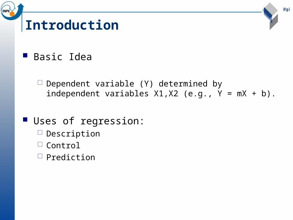
Basic Idea

Dependent variable (Y) determined by independent variables X1,X2 (e.g., Y = mX + b).

Uses of regression: Description Control Prediction

Simple Linear Regression

Yi=0+1Xi +i

Yi value of dependent variable on trial i

0, 1 (unknown parameters)

Xi value of independent variable on trial i

i ith error term (unexplained variation), where

E [i]=0,

2(i)= 2

error terms are N(0, 2)

basic model

iippiii XXXY 22110

• Yi is the ith observation of the dependent variable

• are parameters

• are observations of the ind variables

• are independent and normal

p ,......,0

ipi XX ,........,1

i ),0( 2

iii

ippii

YY

XbXbXbbY

ˆ

ˆ22110

Multiple Regression

BasicModel

estimated model

ith residual

Sometimes we need to transform the data

Predicted versus Observed Plots: (a) model with variables not transformed): R2 = 0.61; (b) Model 7: R2 = 0.85.

Scatter plots: (a) Y versus PORC3_NR (percentage of large farms in number ); (b) log10 Y versus log 10 (PORC3_NR).

Precision of estimates and fitAnalysis of variationSum of squares of Y = Sum of squares of estimate + Sum of

squares of residuals

2ii

2i

2

i)Y(Y)YY()Y(Y ˆˆ

Dividing both sides by TSS (sum of squares of Y):1 = ESS/TSS + RSS/TSS

where ESS/TSS = r2 (coefficient of determination) r2 gives the proportion of total variation

“explained” by the sample regression equation. The closer is r2 to 1.00, the better the fit.

Analysis of Residuals

It is a good idea to plot the residuals against the independent variables to see if they show a trend.

Possible behaviors:Correlation (e.g., the higher the independent variable,

the higher the residual)NonlinearityHeteroskedacity (i.e., the variance of the residual

increases or decreases with the independent variable). Regression assumes that residuals are constant

variance and normally distributed.

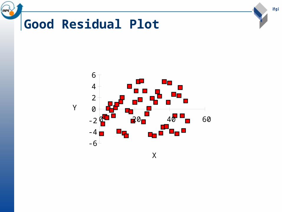
Good Residual Plot

-6

-4

-2

0

2

4

6

0 20 40 60

X

Y

Nonlinearity

-0.15-0.1

-0.050

0.050.1

0.150.2

0.25

0 20 40 60

X

residual

Heteroskedacity

-1

-0.5

0

0.5

1

0 20 40 60

residual

X

Regression with Spatial Data: Understanding Deforestation in Amazonia

The forest...

The rains...

The rivers...

Deforestation...

Fire...

Fire...

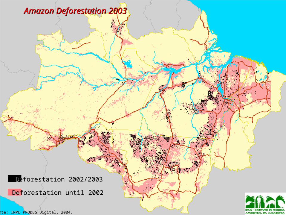
Amazon Deforestation 2003Amazon Deforestation 2003

Fonte: INPE PRODES Digital, 2004.Fonte: INPE PRODES Digital, 2004.

Deforestation 2002/2003Deforestation 2002/2003

Deforestation until 2002Deforestation until 2002

What Drives Tropical Deforestation?

Underlying Factorsdriving proximate causes

Causative interlinkages atproximate/underlying levels

Internal drivers

*If less than 5%of cases,not depicted here.

source:Geist &Lambin

5% 10% 50%

% of the cases

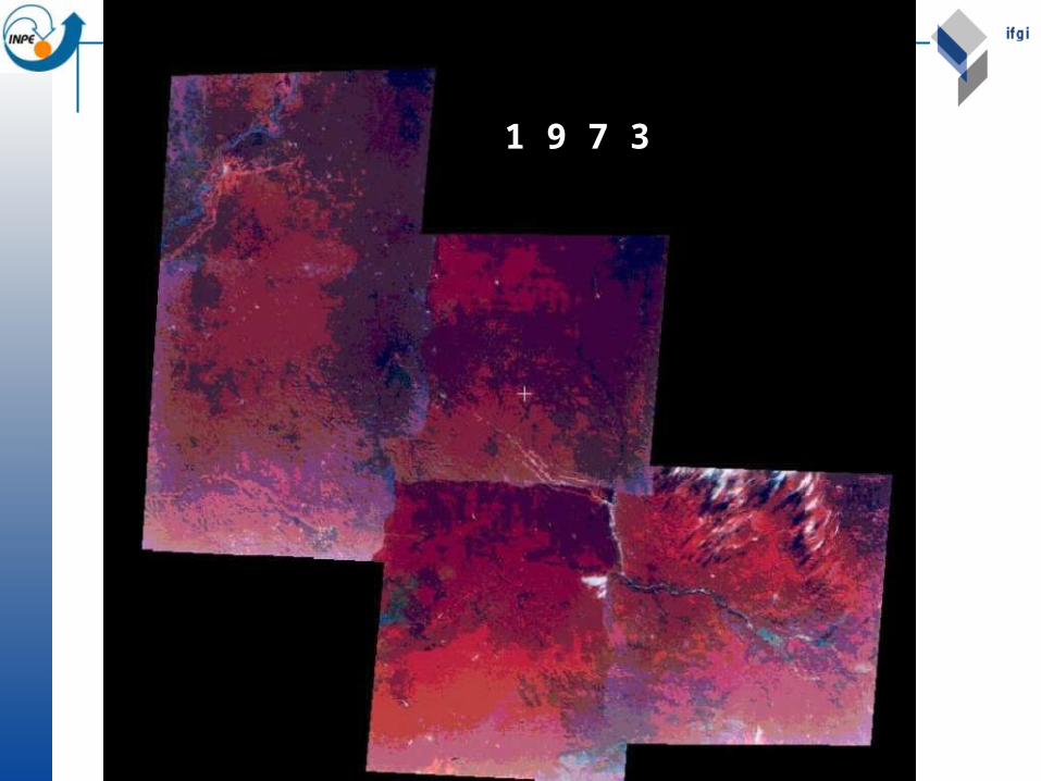
1 9 7 3

1 9 9 1C

ourt

esy:

IN

PE

/OB

T

1 9 9 9C

ourt

esy:

IN

PE

/OB

T

Deforestation in Amazonia

PRODES (Total 1997) = 532.086 km2PRODES (Total 2001) = 607.957 km2

Modelling Tropical Deforestation

Fine: 25 km x 25 km grid

Coarse: 100 km x 100 km grid

•Análise de tendências•Modelos econômicos

Amazônia in 2015? fonte: Aguiar et al., 2004

Factors Affecting Deforestation

Category VariablesDemographic Population Density

Proportion of urban populationProportion of migrant population (before 1991, from 1991 to 1996)

Technology Number of tractors per number of farmsPercentage of farms with technical assistance

Agrarian strutucture Percentage of small, medium and large properties in terms of areaPercentage of small, medium and large properties in terms of number

Infra-structure Distance to paved and non-paved roadsDistance to urban centersDistance to ports

Economy Distance to wood extraction polesDistance to mining activities in operation (*)Connection index to national markets

Political Percentage cover of protected areas (National Forests, Reserves, Presence of INCRA settlementsNumber of families settled (*)

Environmental Soils (classes of fertility, texture, slope)Climatic (avarage precipitation, temperature*, relative umidity*)

Coarse resolution: candidate models

MODEL 7: R² = .86Variables Description stb p-level

PORC3_ARPercentage of large farms, in terms of area 0,27 0,00

LOG_DENS Population density (log 10) 0,38 0,00

PRECIPIT Avarege precipitation -0,32 0,00

LOG_NR1Percentage of small farms, in terms of number (log 10) 0,29 0,00

DIST_EST Distance to roads -0,10 0,00

LOG2_FER Percentage of medium fertility soil (log 10) -0,06 0,01

PORC1_UC Percantage of Indigenous land -0,06 0,01

MODEL 4: R² = .83Variables Description stb p-level

CONEX_ME Connectivity to national markets index 0,26 0,00

LOG_DENS Population density (log 10) 0,41 0,00

LOG_NR1Percentage of small farms, in terms of number (log 10) 0,38 0,00

PORC1_ARPercentage of small farms, in terms of area -0,37 0,00

LOG_MIG2Percentage of migrant population from 91 to 96 (log 10) 0,12 0,00

LOG2_FER Percentage of medium fertility soil (log 10) -0,06 0,01

Coarse resolution: Hot-spots map

Terra do Meio, Pará State

South of Amazonas State

Hot-spots map for Model 7:(lighter cells have regression residual < -0.4)

Modelling Deforestation in Amazonia

High coefficients of multiple determination were obtained on all models built (R2 from 0.80 to 0.86).

The main factors identified were: Population density; Connection to national markets; Climatic conditions; Indicators related to land distribution between large and small

farmers.

The main current agricultural frontier areas, in Pará and Amazonas States, where intense deforestation processes are taking place now were correctly identified as hot-spots of change. 

Spatial regression models

Spatial regression

Specifying the Structure of Spatial dependence which locations/observations interact

Testing for the Presence of Spatial Dependence what type of dependence, what is the alternative

Estimating Models with Spatial Dependence spatial lag, spatial error, higher order

Spatial Prediction interpolation, missing values

source: Luc Anselin

Nonspatial regression

Objective Predict the behaviour of a response variable, given a

set of known factors (explanatory variables).

Multivariate nonspatial modelsyk = 0 + 1x1k +… + ixik + i yk = estimate of response variable for object k i = regression coefficient for factor i xi = explanatory variable i for region k k = random error

Adjustment quality

R2 = 1 –(yi – yi)

i = 1

n

(yi – yi)i = 1

n 2

2

Nonspatial regression: hypotheses

Y = X + (model)

Explanatory variables are linearly independent Y - vector of samples of response variable (n x 1) X – matrix of explanatory variables (n x k) - coefficient vector (k x 1) - error vector (n x 1)

E(i ) = 0 ( expected value) i ~ N( 0, i

2 ) (normal distribution)

Generalized linear models

g(Y) = X + U

Response is some function of the explanatory variables g(.) is a link function Ex: logarithm function

U = error vector (U) = 0 (expected value) (UUT

) = C (covariance matrix) if C= 2 I, the error is homoskedastic

Spatial regression

Spatial effects What happens if the original data is spatially

autocorrelated? The results will be influenced, showing statistical

associated where there is none

How can we evaluate the spatial effects? Measure the spatial autocorrelation (Moran’s I) of the

regression residuals

Regression using spatial data

Try a linear model first

Adjust the model and calculate residuals

Are the residuals spatially autocorrelated? No, we’re OK Yes, nonspatial model will be biased and we should propose

a spatial model

itii xy

iii yyr ˆ

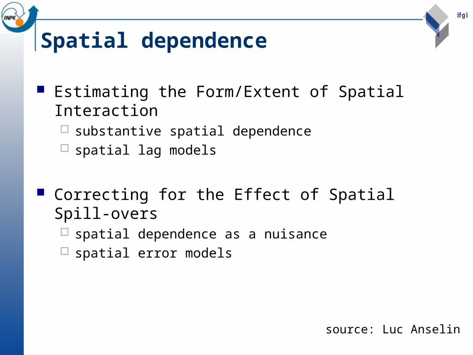
Spatial dependence

Estimating the Form/Extent of Spatial Interaction substantive spatial dependence spatial lag models

Correcting for the Effect of Spatial Spill-overs spatial dependence as a nuisance spatial error models

source: Luc Anselin

Spatial dependence

Substantive Spatial Dependence lag dependence include Wy as explanatory variable in regression y = ρWy + Xβ + ε

Dependence as a Nuisance error dependence non-spherical error variance E[εε’] = Ω where Ω incorporates dependence structure

Interpretation of spatial lag

True Contagion related to economic-behavioral process only meaningful if areal units appropriate (ecological

fallacy) interesting economic interpretation (substantive)

Apparent Contagion scale problem, spatial filtering

source: Luc Anselin

Interpretation of Spatial Error

Spill-Over in “Ignored” Variables poor match process with unit of observation or level of

aggregation apparent contagion: regional structural change economic interpretation less interesting nuisance

parameter

Common in Empirical Practice

source: Luc Anselin

Cost of ignoring spatial dependence

Ignoring Spatial Lag omitted variable problem OLS estimates biased and inconsistent

Ignoring Spatial Error efficiency problem OLS still unbiased, but inefficient OLS standard errors and t-tests biased

source: Luc Anselin

Spatial regression models

Incorporate spatial dependency Spatial lag model

Two explanatory terms One is the variable at the neighborhood Second is the other variables

iti

jjiji xywy

Spatial regimes

Extension of the non-spatial regression model

Considers “clusters” of areas

Groups each “cluster” in a different explanatory variableyi = 0 + 1x1 +… + ixi + i

Gets different parameters for each “cluster”

A study of the spatially varying relationship between homicide rates and socio-economic data of São Paulo using GWR

Frederico Roman RamosCEDEST/Brasil

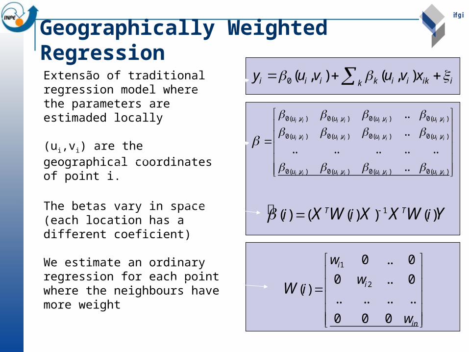
0 ( , ) ( , )i i i k i i ik iky u v u v x

0( , ) 0( , ) 0( , ) 0( , )

0( , ) 0( , ) 0( , ) 0( , )

0( , ) 0( , ) 0( , ) 0( , )

..

..

.. .. .. .. ..

..

i i i i i i i i

i i i i i i i i

i i i i i i i i

u v u v u v u v

u v u v u v u v

u v u v u v u v

1( ) ( ( ) ) ( )T Ti i iX W X X W Y

1

2

0 .. 0

0 .. 0( )

.. .. .. ..

0 0 0

i

i

in

w

wi

w

W

Extensão of traditional regression model where the parameters are estimaded locally

(ui,vi) are the geographical coordinates of point i.

The betas vary in space (each location has a different coeficient)

We estimate an ordinary regression for each point where the neighbours have more weight

Geographically Weighted Regression

Introducing São Paulo

30 Km

70 Km

Some numbers:

Metropolitan region:

Population: 17,878,703 (ibge,200)

39 municipalities

Municipality of São Paulo:

Population: 10,434,252

HDI_M: 0.841 (pnud, 2000)

96 districts

IEX: 74 out of 96 districts were classified as socially excluded (cedest,2002)

4,637 homicide victims in 2001

Data

##### #

######

###

##

#

#

##

#

## # #

#

#

###

#

##

# ##

#

##

#

#

#

##

####

###

#

##

##

#

#

# ##

##

##

#

##

#

#

#

#

##

##

#

###

#

#

###

###

#

#

###

##

##

#

#

#

#

###

#

###

#

#

#####

#

##

# ####

#

# #####

#

#

#

## #

#

# #

#

#

######

#

##

# #

#

#

##

#

###

## ## # #

###

#

## ##

#

#

#

##

#

####

# ###

####

### #

#### ##

#

#######

####

# ####### #

#

##

## #

##

#

####

## ## ##

##

### #

#

#

#

## ##

#

#

#

## #

###

##

#

##

###

#

#

#

#

###

##

##

#

#

##

####

###

#

#

##

###

#

##

#

### ##

#

#

####

#

###

##

#

# #

# ##

#

##

#

####

####

##

#

#

## #

###

#

#

#

#

#

#

#

###

#

###### #

#

##

#

#

####

#

#

#

#

#

##

###

##

######

#

#

##

#

#

#

#

#

#

###

###

#

#

###

#

#

#

#

##

##

#

#

##

# #

#

##

##

###

#

#

#

#####

#

#

#

#

###

##

######

### #

##

###

# # ##

##

#

###

#

#

## # ##

# ##

#

#

#

######

###

#

####

##

## ###

###

##

##

#

####

###

#

###

### ###

## ####

##

#

#

### ## ### ##

## # ###

####

##

#

#

##

#

#

#

##

#

# ##

##

#

###

###

#

#

###

#

#

#

#

##

##

#

#

###

###

#

#

#

#

##

##

###

###

#

##

###

# ##

# ##

##

#

#

#### #

# ##

#

##### # ##

#

##

## #

##

############

#####

## ###

# ##

#

#

#

#

#

#

####

#

#

####

##

#

##

##

# ###

# ####

#######

##

## ##

########### #

## ## #

##### ######

### #

###

##

##

##

##

####

###

##

#

##

####

###

#

#

#

##

#

##

#

###

##

###

###

## ##

##

##

###

####

#

##

###

#

##

##

##

#

#

#

##

#### ##

##

#

##

##

#

##

##

##

##

#

### ## ## ####

#

#

#

#

#

##

##

# ### #

#

#

## ### ##### # #

###

###

####

#

#

##

###

#

#

##

####

#

##

#

##

##

# ###

#

## ##

##

# # #

#

#

#

#

# #

##

#

#

##

## ##

#

#

#####

#

# #

#

##

##

#

##

#

#

## ####

#

##

#

#

#

# # ## ####

#

#### #

# #

#

#

#

#

#

#

####

#

# ###

#

#

##

#

#

###

# #

# # ###

### ## # ####

#

# ###

##

####

##

##

#

#

#

#

##

#

#

## #

#

##

#####

#

##

##

###

# ##

#

#

#

###

#

#

#

##

#

#

## #####

#

##

###

#

#

##

####

##

#

#

## #

##

##

##

#

#

#

##

# #

##

##

#

###

## ##

##

# ## #

#

## #

# #

#

## ## #

#

#

# # ##

#

## #

#

#

# ###

#

# #

#

#

#

##

##

# # #

#

# #

#

##

#######

## #

###

####

###

###

#

#

#

#

#

###

##

#####

#

# ###

# # ###

#

########## #

##

#####

###

#

#

#

#

#### #

#

## #

#

#

#

### ##

#

##

##

##

##

#

#

###

###

##

##

#

##

##

##

###

###

#

#######

#

###

##

###

##

###

##

##

#

##

#

# ##

##

###

####

#

#

####

###

#####

##

###

#

#

#

##

###

#

#

###

#

#

#### #########

#

#####

###

###

# #

## # #

#

##

## #

#

#

####

#

###

###

#

#

#

#

###

##

##

###

#

#

###

# ##

##

#

#

###

##

#

##

##

#

####

# #

##

#

#

##

###### ##

########

####

### ### #

#

## #### ###

####### ## #

##

## #### ####

###

#####

#

### #

#

##

# #

#

#

#

####

#

#

#

#

##

###

##

#

# ### #

#

#

#

#####

##

# ## #

##

#

#

### #

##

#

#

#

##

#

##

#

##

###

# ###

#

#########

#

#####

### # ###

######

###### ###

#

#

##

#

###

#

# #### ## ##

####

##

#

#

#

#

###

#####

#

#

#

###

#

##

##

##

#

###

#

#

#

#

#

#

#

#

#

###

#

###

###

# ###

##

###

#

###

##

#

##

#

##

## ##

#####

##

#####

##

#

#

###

##### ##

#

##

# ## ##

####

#

# ###

###

##

##

# #

## ##

###

#

#

##

#

##

#

#

#

#

#

###

#

########

#

#####

#

#

##

##

#

##### #

#

###

###

#

######

# ### ####### # # ##

###

# #######

####

# ##

##

##

####

#

#### ##

#

## ##### ##

#####

####

######

#

##

# ###

#

####

###

#

##

# # ###

###

##

#############

#

# ##

####

#

##

## #### #

#

#

#

###

# ####

##

#########

# ##

#

### ##

#

#######

########

#

#

###

#

##

# #

##

#

##

#

###

#

##

# #

# #

#

#

#

###

# #

##

#

####### #

###

# ## #####

#

### #### ### #

##

# ## ##

#

#####

#

#

# ####

#####

# ## #

#

##

#

##

##

#

# #

#

###

#

#

### #

#

#

#

#

#

#

##

#

#

#

##

#

####

##

#

#

# #

#

#

####

#

#

#

#

#

###

#

#

#

# #

#

#

#

# #

#

#

## #

#

#

#

###

## ### #

#

#

####

#

#

##

#

#

#

#

###

#####

## #

#

##

#

##

##

####### ##

#

#####

#

#

#

#

##

#

#

#

#

##

###

###

##

####

######## ##

## ##

# #

#####

##

#

#

##

#### #

#######

#

####

##

#

#

# ##

## #

#### ## #####

####

#

#

#

###

###

### ###

#####

###

##

## ## ## #

### ## ### ###

####

#

###

###

#

#

###

###

#

#

##

#########

# ###

###

#

#

#

#

#

###

####

# ##

# #

##

##

#####

#

###

#

#

## ##

#### ####

#

##

# ### #

#

##

#

# ###########

##

##

#

# ##

#####

#

## #

#

#

#

##

##

#

###

#

#

#

#### #####

# #######

###

# ##

##

##

### #

###

##

##

#

#

#

#

##

#

##

###

#

###

##

####

#

#

## #

# #

#

###

#

##

### ##

#

##

######

#

#

#

#

#

#

##

#

#

#

##

#

#

#

# #

#####

##

###

#

# #

##

#

##

#

# #

#

#

#

#

###

#

#

#

#

#

###

###

#

#

## #

#

######## ####

#

##

#

#

##

###

#

#

##

## ###

###

##

#

#

##

# ##

# ###

# ####

#

#

##

#

###

###

#

#

####### # ## #

###########

#########

##

########

##

###

#

###

####

##### #

####

##

#

####

##

#########

## ##

##

###

####

###

#

#

###

##

### ###

#

#

#

#

#

####

#

#

##

#

#

#

#

#

#

##

##

##

#

#

#

##

#

#

#

#

#

#

#

#

#

##

#

#

##

###

#

#

##

## #

##

# #####

##

##

##

##

#

#

###

###

#

####

##

## ##

#

#

###

#####

##

####

#

#

###

##

#

#

##

#

###

###

#

#

#

#

###

#

#

#

## #

#

## #

#

####

#

#

# #

##

###

#

#

##

##

##

#

##

####

#

####

##

#

#

#

#

##

#

#

#

#

##

## ## #

##

#

#

##

#

## ##

###

###

#

##

#

#

#

#

#

#

###

#

#

##

#

#

######

##

#

#

#

# ###

###

#

#

#

#

###

#

##

#

##

#

#

#

#

#

##

### ####

#

##

##### #

##

##

#

# #

# #

##

##

###

# #

#

##

#

#

###

#

#

##

####

#

#

#######

##

####

#

## #

#####

###### #####

##### ##

###

#

#########

##

##

###

#####

#

##

#

#####

#####

#

## ##

#

#

###

### ##

#

##

### #

## ## ###

#

##

#

#####

# #

###

##

#

###

### ########

# ###

##

###

###

######### #

#

### ###

#

#

##

#

###

######

#

#

##

#### #

###

####

#

##

### ##

#

##

# #

#

##

#

###

##

####

#

####

##########

#### ######

###

##

### #### #

## ### #

####

##

#

####

#####

######## #

#

### #

# ###

########

## #

#

# # #

#####

# #

#

###

##

####

#

## ####

##

##

## ##

#####

###

#

##

#

##

#### #

# ###

## ##

#### ##

##

### ####

#

#

####

#

#

# #

#

## ##

#

#

#

#

##

##

##

#

#

##

#

##

###

#

####

## #

##

#

# #

##

# #

##

##

#

#

##

# ## ##

#

####

#

##

## ##

#

#

## #

#

#

#

#

## ##

### #

##

# ### #

##

###

###

### ### ##

##

#

###

#

#

###

#

#

### ###

#

#

#

####

#

##

#

##

##

####

#

#

### #

#

#

##

#

##

###

#

#

# #

#

##

##

# #

###

#

#

#

#

##

##

##

###

#

#

##

#

#

##

#

#

#

#

#

#

#

#

# #

#####

#

###

#

#

##

#

###

##

#

#

#

#

#

#

#

###

#

#

#

#

###

## #

#

#

#

##

# ##

#

#

###

##

##

## #

###

#

#####

####

####

##

###

#

#

#

##

#

#

#

##

### #

#

#

##

#

#

###

#

#

#

#

#

##

###

##

#

# #

#

#

#

##

#

##

#

#

#

# ###

##

#

##

#

####

#

# #

## #

## #

#

#

# # ##

#

###

# ###

## ##

#

#

###

#

#

##

## #

##

#####

#

#

#

###

##

##

###

# ###

#

#

#######

#

##

##

##

####

#

#####

#

#

#

####

###

#

#

#

#

#

#

#

#

#

#

# #

# #

#

#

#

#

# #####

######

##

##

#

####

##

#

#

#

#

###

#

#

#

#

#

##

##

##

#

#

#

####

###

#

##

### ####

#

#

#

#

#

###

#

##

######

#

#

#

#

###

#

#

####

##

## ### ##

#

#

#

#

###

#

#

##

##

#

#

#

#

## ###

#####

##### #

## ####

#

#

##

#

# #

#

#

#

#

##

##

###

#

###

#

##

### #

#

#

#

#####

#

##

##

#

###

#

####

#

#

# #### ###

## # #### ####

#

#

####

######

##

#

##

##

#

#

#

#

#

###

##

###

#

# ##

# #

#

#

######

#

######

###

#

####

#

# #

##

##

#

#

#

##

#

#

#

## #

#

###

#

#

##

###

#

##

#### #

##

### #

##

#

#

#

#

##

#

#

#

####

##

#

#

#

##

#

#

#

#

#

#

###

# ##

# # ###

#

##

#

###

# ##

## ###

###

#

#

#

###

### # ##

##

#

# #

#

####

#

#

#

##

#

##

##

#

#

#

##

#

#

#

##

##

##

#

##

##

#

#

#

##

##

###

#

#

##

# #

#

#

###

###

###

#

#######

#

#

####

##

## ##

#

# ## ###

# ####### #

#####

##

#

#

#

##

#

#

###

#

#

#

#

#

#

###

4,637 homicide victimsresidence geoadressed2001

456 Census Sample Tracts2000

######

########

###

#

#

##

#

## ##

#

#

###

#

##

####

###

#

#

##

####

###

#

###

##

#

###

##

###

##

#

#

##

####

#

###

#

#

######

##

#####

##

#

##

#

###

##

####

######

### #

####

##

#####

#

#

## #

#

# #

#

#

#######

##

##

#

###

#

###

## ##

# ### #

#

##

##

#

#

#

###

####

# ###

####

####

#### ##

#

#######

####

# ####### #

#

##

###

##

#

####

## ####

##### ##

##

####

#

##

##

##

####

#

#####

##

##

###

###

#

#

#

##

###

#######

###

##

###

#####

#

#

#####

###

##

## #

# ##

#

###

####

####

##

#

#

###

###

##

#

#

#

#

#####

###### #

###

#

#

####

#

#

#

#

##

#

###

##

######

#

#

##

#

##

#

#

#

###

###

#

#

###

##

##

##

###

###

# ##

##

#####

#

#

#####

#

#

##

#

###

##

######

####

##

####

#####

#

###

#

### # ##

# ##

##

#

#########

####

###

#####

#####

###

####

####

###

######

## ###

###

##

##### ### ##

## #

#######

##

##

##

#

#

#

#### #

#

##

##

##

####

#

####

##

#

##

###

#

###

###

#

##

#

##

####

#

###

#

###

#####

# ##

###

### ###

###

#########

###

## #

####

########

##

######

####

###

##

#

#

#

#

####

#

#

###

###

###

#####

## #

###

########

### ###

########## ######

#####

######

####

###

##

##

##

##

####

###

##

#

##

####

###

##

##

#

#

###

###

##

####

##

## ####

#####

####

###

###

#

######

#

#

#

#####

# ##

##

#

##

###

##

##

##

##

#

### ## ## #####

#

#

#

##

##

#

#####

#

### #####

#### ###

###

#

####

#

#

##

###

#

#

######

#

##

##

#

##

####

#

## ##

##

## ##

##

#

##

##

##

######

#

######

#

# #

#

##

##

#

# ##

### ####

#

##

#

#

## # #

######

###### ##

##

#

#

#

####

#

# ####

#

###

#

###

# ## ###

#### ### ####

## ###

##

####

##

###

#

##

##

#

#

## ##

##

###

##

#

##

###

##

# ##

#

#

#

###

##

##

##

#

## ######

##

###

##

##

####

##

#

##

####

##

##

#

#

###

# #

##

##

####

###

###

####

#

## #

# #

### ###

#

#

# #####

# ##

## ##

#

#

# #

#

##

###

#

# # ### #

#

##

#######

## #

###

####

###

###

#

#

#

#

#

###

## ####

#

#

# ###

#####

#

########## #

##

##### ###

##

#

##### #

##

###

##### ##

#

####

##

##

##

###

###

####

#

##

##

##

####

#######

###

#

###

##

###

##

###

####

#

##

#

# ##

##

###

####

#

#

####

####

#####

##

##

##

##

###

##

####

#

#

#### ###

######

##

###

####

###

##

## ###

##

## #

#

#

####

####

###

#

#

#

#

####

#

###

##

#

#

###

# ##

###

#

###

##

#

##

##

####

## #

##

#

#

##

#####

# ##

########

###

###

######## #### ###

####### ## ###

###### #

####

#####

##

#

### #

#

##

# #

##

#####

#

#

#

#

#####

##

#

# ## # ##

#

#

#######

# ###

##

#

#

####

###

#

#

###

###

##

###

# ###

#

##########

#####

##########

######### ###

#

#

##

#

###

#

# ###

########

#

##

#

#

#

######

#####

###

#

###

##

##

#

###

##

#

#

#

#

#

##

####

#####

#

####

##

##

##

###

###

##

#

##

########

########

###

#

#####

######

##

####

#

####

#

# ####

##

##

##

##

## ##

###

##

##

#

##

#

#

#

#

####

#########

#

######

#

##

######

####

###

###

#

########

## ####### ####

###

# #########

### ##

##

##

###

#

#

####

##

### #######

######

#########

###

####

#

####

###

##

###

###

#####

##############

#####

###

##

#####

##

##

####

# ##

##

##

#########

###

#

#####

#

###############

#

#

########

##

#

###

###

###

### #

#

##

#### #

##

#

####

### #

###

# #####

###

### #### ###

###

# ####

#

#####

#

####

##

#####

# ## ##

##

#

##

##

#

##

#

###

##

### #

#

##

#

#

###

#

##

##

#####

##

#

#

# #

#

##

###

#

#

#

##

####

#

## #

##

###

#

#

###

##

#

###

## ####

#

#

####

#

#

##

#

#

#

##

##

####### #

###

#

##

##

#####

## ###

#####

#

#

#

#

####

#

#

##

###

###

##

####

##########

####

# ######

###

##

###

###

########

####

###

#

#####

#

###### #####

#####

#

#

###

#####

###

####

#####

##

#### ## #

##### ### ###

########

####

#

###

###

##

##

##############

###

##

#

#

####

###

# ##

##

##

##

#####

#

###

##

## ##

########

###

#### ##

##

#

# ###########

##

##

## ##

#####

### #

#

#

#

##

###

###

#

##

#### #####

# #######

#### ##

####

####

###

##

##

#

#

#

#

##

###

###

#

###

##

#####

#

## #

# #

#

####

##### #

####

#######

#

#

#

#

#

###

#

#

##

#

##

# #####

#

##

###

#

# #

##

####

##

###

#

###

#

#

#

#

#

###

###

#

#

## #

###

####

######

####

###

####

###

## ######

###

###

###

# ###

# ####

##

###

###

####

##

###### #

##############

#########

##########

##

####

###

####

######

#######

####

##

########

#### #

##

#######

####

##

##

########

#

##

#

#

####

#

#

##

#

#

#

#

#

#

##

##

##

#

#

#

##

#

#

#

#

#

#

#

##

###

#

##

###

##

##

## ###

# #####

##

##

##

##

#

####

###

#####

#### ##

#

###

######

##

####

#

#

###

###

#

##

#

######

#

#

##

###

#

##

## #

#

###

#

#####

#

##

##

###

##

##

##

##

###

####

#

####

##

#

#

#

#

##

##

#

#

##

## ###

##

#

#

##

#

## ####

#

###

#

##

#

#

#

##

#

###

##

##

#

#######

###

#

#####

###

#

#

#

#

###

#

##

###

#

#

##

#########

#

#

##

######

##

###

####

######

###

#

###

####

##

##

####

#

#

########

####

###

######

#

###### #####

##### #

####

#

#########

# ###

#####

###

#########

#####

#####

##

###

### #####

####

## ## ####

##

#

#####

# ####

##

####

###########

####

#####

###

######### ##

### ###

#####

###

######

#

#

##

#### ##

##

#######

### ##

###

##

###

#

#######

###

##############

##########

#############

## ####

####

##

#

####

#####

######## ##

####

########## #

#

## ##

# #######

##

####

######

##

#####

##

##

########

#

####

###

####

#### ###

####

#### ####

#######

#

#

####

##

# #

### #

#

#

##

###

###

#

#

#

##

#

#####

#

####

###

##

#

# #

##

# #

##

##

#

###### #

#

#

## ###

######

#

#

## #

##

##

####

####

##

#### #

##

###

###

### #####

###

###

##

###

#

##

## #####

#

###

#

#

###

##

#######

##

## #

#

#

##

#

##

###

#

###

##

## #

# #

####

#

#

#

##

##

####

##

#

##

#

#

##

#

#

#

##

#

#

###

######

###

#

##

#

#

###

##

#

##

#

#

#

#

###

#

#

##

###

## #

#

#

###

##

#

##

###

####

## ####

#

#####

####

####

###

###

#

#

##

#

##

##

####

##

###

####

#

#

#

#

###

# ####

#

# ##

#

#

##

#

##

#

#

#

# ###

##

###

#

####

#

# ####

## #

#

#

# # ##

##

##

# ###

#####

##

##

#

###

###

#####

##

#

##

###

##

##

###

# ####

########

#

####

##

####

#

######

#

###

##

##

#

##

#

##

#

##

#

#

# ## #

#

#

##

# #####

######

##

##

#

#####

#

##

#

#

###

##

#

##

##

##

###

#

#

####

###

###

#######

#

#

#

#

#

###

##

#####

##

#

#

##

###

#

#

####

#### ### ##

#

##

#

###

#

##

#

##

##

#

#

###

##

#####

#####

#

######

##

##

## #

#

#

##

##

##

###

##

##

##

##

#####

######

#

##

###

#####

###

#

###### ###

###

########

#

#

###

#

######

##

#

###

##

#

#

#

#

###

##

###

## #

###

##

##########

###

###

#####

## ###

##

#

#

#

##

##

#

###

#

###

#

#

#####

#

##

###

##

####

###

##

#

#

###

#

#

##

### ##

#

##

##

#

#

#

##

####

# ### # #

##

##

##

###

###

#####

###

#

#

####

####

####

#

##

#

####

#

#

#

##

#

##

###

#

#

###

#

#

##

##

##

###

###

#

#

##

##

###

#

#

##

# #

#

#

###

###

###

######

##

#

#

######

## ##

## ## ##

######

### ######

###

#

###

##

###

#

#

#

#

#

#

###

Density surface of victim-based homicides

Kernel Density Function

Bandwidth = 3 Km

Critical areas Critical areas

Critical areas

Victim-based homicide rate (Tx_homic)

0

10

20

30

40

50

60

70

Tx_homic

Tx_homic = count homicide events (2001) *100.000 population (census, 2000)

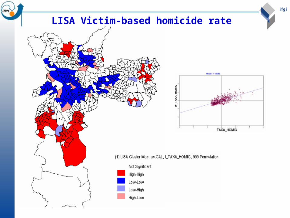
LISA Victim-based homicide rate

Percentage of illiterate house-head (Xanlf)

0

10

20

30

40

50

60

DefinitionHouse-head is the person responsible for the house. Generally, but not necessarily, who has the highest income of the house

LISA Percentage of illiterate house-head

OLS regression results for TX_homic and X_analf

Model Summaryb

,598a ,357 ,356 22,5033Model1

R R SquareAdjustedR Square

Std. Error ofthe Estimate

Predictors: (Constant), XNALFa.

Dependent Variable: TAXA_HOMICb.

ANOVAb

124145,0 1 124144,979 245,153 ,000a

223321,9 441 506,399

347466,9 442

Regression

Residual

Total

Model1

Sum ofSquares df Mean Square F Sig.

Predictors: (Constant), XNALFa.

Dependent Variable: TAXA_HOMICb.

Coefficientsa

16,064 1,997 8,043 ,000

4,566 ,292 ,598 15,657 ,000

(Constant)

XNALF

Model1

B Std. Error

UnstandardizedCoefficients

Beta

Standardized

Coefficients

t Sig.

Dependent Variable: TAXA_HOMICa.

OLS regression results for TX_homic and X_analf

Linear Regression

0,00000 5,00000 10,00000 15,00000 20,00000

xnalf

0,00

50,00

100,00

150,00

TAX

A_H

OM

IC

TAXA_HOMIC = 16.06 + 4.57 * xnalfR-Square = 0.36

5 0 5 10 15 Kilometers

Area_ po.shp< -3 Std. Dev.-3 - -2 Std. Dev.-2 - -1 Std. Dev.-1 - 0 Std. Dev.Mean0 - 1 Std. Dev.1 - 2 Std. Dev.2 - 3 Std. Dev.> 3 Std. Dev.

View1

Moran=0,2624

LISA for standardized residuals of the OLS regression for TX_homic and X_analf

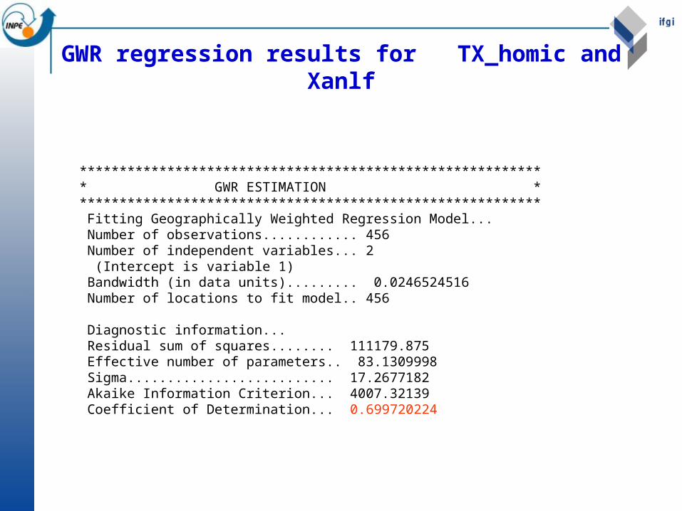
*********************************************************** GWR ESTIMATION *********************************************************** Fitting Geographically Weighted Regression Model... Number of observations............ 456 Number of independent variables... 2 (Intercept is variable 1) Bandwidth (in data units)......... 0.0246524516 Number of locations to fit model.. 456 Diagnostic information... Residual sum of squares........ 111179.875 Effective number of parameters.. 83.1309998 Sigma.......................... 17.2677182 Akaike Information Criterion... 4007.32139 Coefficient of Determination... 0.699720224

GWR regression results for TX_homic and Xanlf

Moran= -0,0303

GWR regression results for TX_homic and Xanlf

residuals

5 0 5 10 Kilometers

Area_ po.shp-6.396 - -1.855-1.855 - 00 - 3.5323.532 - 5.8435.843 - 15.765

GWR regression results for TX_homic and Xanlf

Local Beta1 Local t-value

CONCLUSIONS

-There are significant differences in the relationship between violence rates and social territorial data over the intra-urban area of São Paulo

-This results reinforces our hypotheses that we should avoid using general concepts

-The GWR technique is a useful instrument in social territorial analysis